Site-dependent control of polaritons in the Jaynes–Cummings–Hubbard model with trapped ions

Abstract

We demonstrate the site-dependent control of polaritons in the Jaynes–Cummings–Hubbard (JCH) model with trapped ions. In a linear ion crystal under illumination by optical beams nearly resonant to the red-sideband (RSB) transition for the radial vibrational direction, quasiparticles called polaritonic excitations or polaritons, each being a superposition of one internal excitation and one vibrational quantum (phonon), can exist as conserved particles. Polaritons can freely hop between ion sites in a homogeneous configuration, while their motion can be externally controlled by modifying the parameters for the optical beams site-dependently. We demonstrate the blockade of polariton hopping in a system of two ions by the individual control of the frequency of the optical beams illuminating each ion. A JCH system consisting of polaritons in a large number of ion sites can be considered an artificial many-body system of interacting particles, and the technique introduced here can be used to exert fine local control over such a system, enabling detailed studies of both its quasi-static and dynamic properties.

1 Introduction

Recent advancements in quantum information science and associated technologies have led to the development of quantum information processing, including quantum computation and quantum simulations Feynman (1982); Blatt and Roos (2012); Cirac and Zoller (2012); Daley et al. (2022). In quantum simulations, physical systems that approximately simulate naturally existing systems, as well as artificially designed systems, which may have similarities with existing systems, are realized in a well-controlled physical platform, and their properties can be studied. The Jaynes–Cummings–Hubbard (JCH) model Greentree et al. (2006); Hartmann et al. (2006); Angelakis et al. (2007); Ivanov et al. (2009) is simulable in various physical platforms. The model comprises an array of Jaynes–Cummings (JC) systems Jaynes and Cummings (1963), where each JC system consists of an atom-like two-level system (TLS) and a harmonic oscillator comprising a single mode of a quantized wave field. In a system obeying the JCH model, a strongly interacting system of quasiparticles called polaritons is expected to be realized, where each polariton is a superposition of an excitation in the TLS and a wave quantum such as a photon or a phonon.

The JCH model was initially proposed for an array of coupled optical cavities, such as photonic band gap cavities, each containing a single two-level atom Greentree et al. (2006). The model has been applied to other systems including superconducting systems Hoffman et al. (2011); Raftery et al. (2014); Fitzpatrick et al. (2017) and trapped ions Ivanov et al. (2009); Toyoda et al. (2013); Debnath et al. (2018); Li et al. (2022). These systems share similar properties with respect to their controllability, including the site-dependent control of the model parameters. In the case of a JCH system of trapped ions Ivanov et al. (2009), the ions are illuminated with optical beams nearly resonant to the red-sideband transition for a vibrational direction, and the parameters for the optical beams, especially their amplitudes and frequencies, determine important system parameters such as the site-wise JC coupling constants and detunings of the wave fields with respect to the TLS resonances. Angelakis et al. Angelakis et al. (2007) and Ivanov et al. Ivanov et al. (2009) found that by varying the global detuning, a quantum phase transition (or crossover) between a Mott-insulator and superfluid states can be observed. This has been reproduced in experiments observing a phase crossover Toyoda et al. (2013), where the variation of the detuning over a relatively large span that exceeds the magnitudes of all the relevant parameters (JC coupling constants and the phonon hopping rate) results in a transition from one characteristic system ground state to another with a completely different character. In another study, site-dependent amplitude variation was utilized to realize control of the hopping of phonons (not polaritons) in a system of three trapped ions Debnath et al. (2018).

In this article, we propose the use of site-dependent frequency shifts for optical beams nearly resonant to the red-sideband (RSB) transition in trapped ions, to control the motion of polaritons in the system. Using this technique, we realize the blockade of polariton hopping in a system of two ion sites. By varying the frequencies of the optical beams, the polariton hopping to or from a particular ion site can be suppressed. Hence, it is possible to effectively decouple one ion site from the system dynamics.

The scheme introduced here is similar to that used in the phonon blockade demonstrated by Debnath et al. Debnath et al. (2018), in that both schemes utilize the discrepancy of the relevant eigenenergies across ion sites to realize the blockade of the motion of quasiparticles (either polaritons or phonons) in a linear ion crystal. In comparison to the scheme in Debnath et al. (2018), we find that in the scheme presented here, the leakage of quasiparticles to the ion site illuminated by the blockade optical beam can be lower by a factor of approximately four in an optimum case, assuming the same RSB Rabi frequency.

The technique presented here can be applied to various studies, and we consider here that of quantum phase crossovers and their dependence on the number of ion sites. There is a certain experimental cost in changing the number of ion sites, since doing this typically requires a reloading (or at least an additive loading when increasing the number). Even a change of the optical beam positions may be required if each ion is addressed with a different beam. By using the technique introduced here, it is possible to decouple some of the ion sites, and hence, effectively reduce the number of ion sites without changing the configuration of the ion crystal itself. This can be done by selectively shifting the optical beam frequencies for the ions placed close to both edges of the linear crystal, where it is assumed that each ion is separately addressed with one dedicated optical beam. In this way, the number dependence of phase crossovers, in analogy to a spin system Islam et al. (2011), can be observed without reloading or additive loading. The technique introduced here can also be applied to studies of dynamical properties Cirac and Zoller (2012); Daley et al. (2022); Wong and Law (2011); Nissen et al. (2012); Li et al. (2021), where strong site-dependent as well as time-dependent disturbances can be applied to the system.

2 Principles of polaritons in the JCH model

In this section, we review the formalism for polaritons in the JCH model. First, the JC Hamiltonian is introduced to describe a single ion site comprising two internal states and a quantized radial vibrational mode (we assume $\hbar=1$ throughout the paper):

$$H_{\mathrm{JC}} = \omega\hat{a}^{\dagger}\hat{a}+(\omega+\Delta_{\mathrm{JC}})\hat{\sigma}^{+}\hat{\sigma}^{-}$$ (1)

$$+g_{\mathrm{JC}}(\hat{a}\hat{\sigma}^{+}+\hat{a}^{\dagger}\hat{\sigma}^{-}).$$

Here, we assume that a laser with a frequency of $\omega_{\mathrm{L}}$ that is nearly resonant to the RSB transition for the radial vibrational motion is applied, and the Hamiltonian is taken in a frame rotating with that frequency. $\omega$ is the vibrational frequency. $\hat{a}^{\dagger}$ and $\hat{a}$ are the creation and annihilation operators for radial phonons, respectively, where the radial phonon states are assumed to be spanned by phonon number states $\ket{n}$ ($n=0,1,\ldots$). $\Delta_{\mathrm{JC}}\equiv(\omega_{0}-\omega)-\omega_{\mathrm{L}}$ is the detuning for the JC coupling, where $\omega_{0}$ is the resonance frequency for the internal states. $\hat{\sigma}^{+}$ and $\hat{\sigma}^{-}$ are the raising and lowering operators for the internal states, respectively, where the internal states are assumed to be spanned by the ground ($\ket{g}$) and excited ($\ket{e}$) states. $g_{\mathrm{JC}}$ is the JC coupling strength, which is dependent on the RSB Rabi frequency. The first term in Eq. (1) corresponds to the phonon energy and the second term to the atomic internal energy. The last term represents the JC coupling induced by the RSB excitation laser. In this system, the concept of dressed atoms Cohen-Tannoudji (2005) emerges, which has a close relation to the polaritons dealt with in this work. The ground state of the combined system ($\ket{0,g}\equiv\ket{0}\otimes\ket{g}$) and the dressed states ($\ket{p,\pm}$) possess the following eigenenergies ($p=1,2,\ldots$):

$$E_{0} = 0,$$ (2)

$$E_{p,\pm} = \omega{p}\pm\Omega_{p}(\Delta),$$ (3)

where $\Omega_{p}(\Delta)=[\Delta^{2}+4g_{\mathrm{JC}}^{2}p)]^{1/2}$ is the generalized Rabi frequency. The eigenenergies of $\ket{1,\pm}$ are plotted against the JC detuning $\Delta_{\mathrm{JC}}$ in Fig. 1.

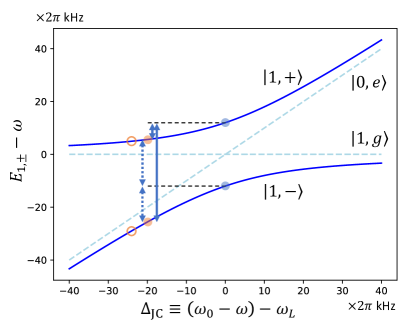
Figure 1: Eigenenergies for dressed states in the JC model. The eigenenergies of the dressed states $\ket{1,\pm}$ are plotted against the JC detuning $\Delta_{\mathrm{JC}}$ as blue solid curves. The energies for the bare states $\ket{1,g},\ket{0,e}$ are plotted as light blue dashed lines. For those eigenenergies, the reference point is taken at $\omega$, which corresponds to the energy of the bare states $\ket{1,g},\ket{0,e}$ at resonance. The blue filled circles represent eigenenergies at resonance, which correspond to those at Ion 1. The red filled circles represent eigenenergies for $\Delta_{\mathrm{JC}}=-2\pi\times 20$ kHz, which correspond to those at Ion 2 in the case shown in Fig. 3(e), (f) and Fig. 4(a). The blue solid arrows (blue dotted arrows) represent the energy gaps between the $\ket{1,+}$ ($\ket{1,-}$) eigenenergy at Ion 1 and eigenenergies at Ion 2. The red hollow circles represent eigenenergies for $\Delta_{\mathrm{JC}}=-2\pi\times 24$ kHz, which corresponds to those at Ion 2 in the case of minimum leakage, as is shown in Fig. 4(b)

The combined system of the internal states of ions in a linear crystal and their vibrational states along a radial direction under the illumination of optical beams nearly resonant to the RSB transition can be described by the JCH model Ivanov et al. (2009). Polaritons in this system can be defined in a way similar to dressed atoms in the single-site case, but with the additional property of being able to propagate within the crystal Ohira et al. (2021), which is inherited from the similar property of radial phonons in a linear ion crystal Porras and Cirac (2004); Haze et al. (2012); Tamura et al. (2020). The JCH Hamiltonian for a linear crystal with $N$ ions is given as

$$H_{\mathrm{JCH}} = \sum_{i=1}^{N}\left[\omega_{i}\hat{a}_{i}^{\dagger}\hat{a}_{i}+(\omega_{i}+\Delta_{\mathrm{JC},i})\hat{\sigma}_{i}^{+}\hat{\sigma}_{i}^{-}\right]$$ (4)

$$+\sum_{i=1}^{N}{g_{i}}(\hat{a}_{i}\hat{\sigma}_{i}^{+}+\hat{a}_{i}^{\dagger}\hat{\sigma}_{i}^{-})$$

$$+\sum_{i<j}^{N}\frac{k_{ij}}{2}(\hat{a}_{i}\hat{a}_{j}^{\dagger}+\hat{a}_{i}^{\dagger}\hat{a}_{j}).$$

Here, $\omega_{i}=\omega-\sum_{i\neq j}^{N}k_{ij}/2$ ($i=1,2,\ldots,N$) is the site-dependent vibrational frequency incorporating inter-ion Coulomb couplings Porras and Cirac (2004); Zhu et al. (2006). $\hat{a}_{i}^{\dagger}$ and $\hat{a}_{i}$ are the creation and annihilation operators for local phonons along the radial direction of the $i$th ion. $\Delta_{\mathrm{JC},i}\equiv(\omega_{0}-\omega_{i})-\omega_{\mathrm{L},i}$ is the site-dependent detuning for the JC coupling, where $\omega_{\mathrm{L},i}$ is the site-dependent frequency of the optical beam illuminating the $i$th ion. $\hat{\sigma}_{i}^{+}$ and $\hat{\sigma}_{i}^{-}$ are the raising and lowering operators for the internal states of the $i$th ion, respectively. $g_{i}$ is the JC coupling strength for each ion site. The last term in Eq. (4) describes the hopping of phonons between different ion sites. $k_{ij}=e^{2}/4\pi\epsilon_{0}md_{ij}^{3}\omega_{i}$ is the hopping rate between the $i$th and $j$th ion sites Porras and Cirac (2004); Haze et al. (2012), where $m$ is the mass of an ion and $d_{ij}$ is the distance between the $i$th and $j$th ions.

In the case of two ions, which is relevant in the present work, the JCH Hamiltonian is as follows:

$$H_{\mathrm{JCH}} = \sum_{i=1}^{2}\left[\omega\hat{a}_{i}^{\dagger}\hat{a}_{i}+(\omega+\Delta_{\mathrm{JC},i})\hat{\sigma}_{i}^{+}\hat{\sigma}_{i}^{-}\right]$$ (5)

$$+\sum_{i=1}^{2}{g_{i}}(\hat{a}_{i}\hat{\sigma}_{i}^{+}+\hat{a}_{i}^{\dagger}\hat{\sigma}_{i}^{-})$$

$$+\frac{k_{12}}{2}(\hat{a}_{1}\hat{a}_{2}^{\dagger}+\hat{a}_{1}^{\dagger}\hat{a}_{2}).$$

Here, the site-dependent corrections for the vibrational frequencies $-\sum_{i\neq j}^{N}k_{ij}/2$ are omitted and each $\omega_{i}$ is represented by the same symbol $\omega$ considering the symmetry in the system.

3 Experimental procedure

In the present experiment, two ⁴⁰Ca⁺ ions are used, which are trapped inside a linear Paul trap with an ac electric field oscillating at 24 MHz and a dc electric field. The single-ion vibrational frequencies for the trap are $(\omega_{x},\omega_{y},\omega_{z})/2\pi=(2.95,2.74,0.18)$ MHz. The distance between the two ions is 18 $\mu$m and the phonon hopping rate is $k_{12}=2\pi\times 5.9$ kHz.

Two lasers at 423 and 370 nm are used for ion loading with optical ionization. Laser beams at 397 and 866 nm, nearly resonant to $S_{1/2}$–$P_{1/2}$ and $D_{3/2}$–$P_{1/2}$, respectively, are used for Doppler cooling. A laser at 729 nm nearly resonant to $D_{5/2}$–$P_{3/2}$ is used for sideband cooling (SBC) and the initialization of a polariton, as well as in the experimental step for the observation of polariton dynamics (we call this the quantum simulation step). The output of the 729-nm laser is divided and two beams are applied to the two ions so that each ion is illuminated with one dedicated beam. The resulting maximum carrier (RSB) Rabi frequency is measured to be $\sim 600$ (24) kHz for each ion. A laser at 854 nm is used to deplete the population in $D_{5/2}$ during SBC and after the manipulation of polaritons. The detection of the internal states is done by illumination with 397- and 866-nm pulses and by collecting fluorescence photons with a photomultiplier tube.

In our setup, the frequencies for the optical pulses at 729 nm illuminating the respective ions (Ions 1 and 2) during the quantum simulation step can be set to be either equal to or different from each other, and in the latter case the finite frequency difference may lead to a blockade of polariton hopping. In the present experiment, the frequency for the pulse illuminating Ion 1 is kept at the resonance of the RSB transition, while that for the pulse illuminating Ion 2 is varied over a certain range.

The frequencies for the optical pulses are controlled using acousto-optic modulators (AOMs) in both double-pass and single-pass configurations. A double-pass AOM system Donley et al. (2005) is used for the base frequency control for all the optical beams at 729 nm, while a single-pass AOM system is used to control the frequency of the respective optical beam illuminating each ion. In contrast to a double-pass configuration, a single-pass configuration enables amplitude/frequency modulation with high efficiency in the diffracted power, though an angle shift of the diffracted beam and a resulting spatial shift of the optical beam at the position of the ions cannot be avoided. In the present experiment with a maximum frequency shift of $\sim$20 kHz, the spatial shift is estimated to be $\sim$0.1 $\mu$m, which is sufficiently small compared with the beam waist size ($e^{-2}$ radius $\sim$3 $\mu$m).

Figure 2 shows the time sequence for the present experiment (after Doppler cooling). As is described above, we use lasers at 397 and 866 nm to perform Doppler cooling. Further cooling is obtained by performing SBC with lasers at 729 and 854 nm, thereby cooling the ions to near the vibrational ground state in the radial directions. The average phonon numbers in the radial directions measured after SBC are $(\langle{n}_{x}\rangle,\langle{n}_{y}\rangle)=(0.30,0.03)$. Then, the initial state for the observation of polariton hopping and a blockade is prepared. This is done by applying a carrier $\pi$ pulse (length $\sim{1}$ $\mu$s) and RSB $\pi/2$ pulse (length $\sim{10}$ $\mu$s) in succession to one of the two ions, which is identified as Ion 1 (and the other as Ion 2). The state in Ion 1 after these is a superposition of $\ket{0,e}\equiv\ket{0}\otimes\ket{e}$ and $\ket{1,g}\equiv\ket{1}\otimes\ket{g}$, where $\ket{g}$ corresponds to the internal ground state ($\ket{S_{1/2},m_{J}=-1/2}$) and $\ket{e}$ to the internal excited state ($\ket{D_{5/2},m_{J^{\prime}}=-1/2}$). This state corresponds to one polariton in Ion 1. The preparation step just described is followed by the quantum simulation step, where the ions are illuminated with RSB optical pulses that have equal intensities with respect to both ions, while their frequencies are adjusted depending on which type of experiment we perform, i.e., without a frequency difference for no blockade and with a finite frequency difference in the case of observing a polariton blockade. The time sequence is repeated while varying the length for the quantum simulation step from zero to a certain length so that the time-dependent behavior of the system is acquired.

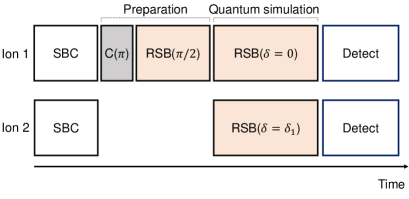
Figure 2: Time sequence for observing polariton blockade by individual control of the optical beam frequency. $\mathrm{C}(\pi)$ represents a carrier $\pi$ pulse. $\mathrm{RSB}(\pi/2)$ represents a resonant RSB pulse with pulse area $\pi/2$. $\mathrm{RSB}(\delta)$ represents either a resonant ($\delta=0$) or off-resonance ($\delta\neq 0$) RSB pulse with a certain length

4 Results

The results for the observation of polariton hopping and the blockade of a polariton using frequency shifts of individually addressing RSB pulses are shown in Fig. 3. In Fig. 3(a), the population in $\ket{e}$ in the case without a frequency difference in the RSB pulses between the two ion sites is plotted against elapsed time. After a polariton is prepared in Ion 1 (before the time $t=0$), it starts hopping to the other ion site (Ion 2) to form a superposition between the two. Still, part of its wave packet remains in the initial ion site for a while ($\sim 100$ $\mu$s), manifesting as a relatively fast oscillation with a period of $\sim$40 $\mu$s. This oscillation is observed because the polariton state does not coincide with one of the eigenstates of the instantaneous JC Hamiltonian under the illumination of the RSB pulses, but in fact corresponds to a superposition of eigenstates, that is, $\ket{1,+}$ and $\ket{1,-}$, and the interference between these two states generates the relatively fast oscillation in the population observed before $t=100$ $\mu$s. We can also describe the fast oscillation as a sideband Rabi oscillation induced by the RSB pulse. In any case, the structure can be understood as local time-dependent behavior within one ion site. Eventually, the polariton moves to Ion 2, which is confirmed by the oscillatory behavior observed for Ion 2 in $t=0$–$300$ $\mu$s. From around $t$ = 200 $\mu$s, a similar oscillatory behavior is again seen in Ion 1 (along with larger noise), which corresponds to the wave packet returning to the original ion site. In this way, the polariton goes back and forth between the two ion sites, and this behavior is confirmed in the envelopes of the populations in Ions 1 and 2, which again show oscillatory behaviors with a longer period of $\sim$340 $\mu$s. The oscillations in the envelopes show relaxations due to decoherence in the system. The decoherence can be ascribed to such factors as intensity fluctuations of the optical beam and associated frequency fluctuations due to AC Stark shifts, as well the finite temperature after performing SBC. The causes for the decoherence in our system are discussed in more detail in Ohira et al. (2022).

A numerically calculated result corresponding to the experimental result in Fig. 3(a) is shown in Fig. 3(b). In the numerical calculation, we assume $2g_{1}=2g_{2}=2\pi\times 24$ kHz and $k_{12}=2\pi\times 5.9$ kHz. We also incorporate the error due to the decoherence Ohira et al. (2022). For this, we assume a thermal distribution in the radial $y$ direction with $\langle{n}_{y}\rangle=0.03$, and relative intensity fluctuations with a standard deviation of $\sim 0.02$. It is confirmed from the results that the qualitative behavior of the experimental result is well reproduced in the calculated result.

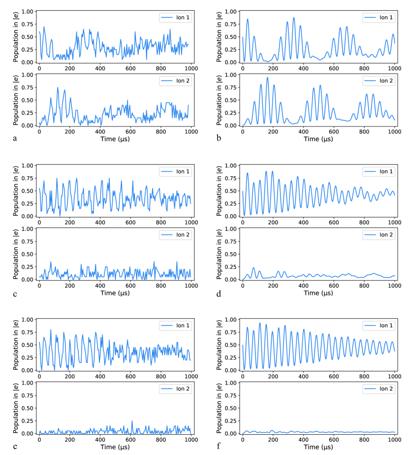
Figure 3: Observation of polariton hopping and its blockade by illuminating individually addressed RSB optical pulses with site-dependent frequency shifts. (a) Experimental result for zero detuning ($\Delta_{\mathrm{JC},2}=0$) and (b) corresponding numerically calculated result, where a relatively fast oscillation with a period of $\sim$40 $\mu$s and a relatively slow change of the envelope with the period of $\sim$350 $\mu$s can be seen. (c) Experimental result for $\Delta_{\mathrm{JC},2}=-2\pi\times 10$ kHz and (d) corresponding numerical result, where a relatively fast oscillation still exists while the relatively slow oscillation of the envelope is not apparent. (e) Experimental result for $\Delta_{\mathrm{JC},2}=-2\pi\times 20$ kHz and (f) corresponding numerical result, where again the relatively slow oscillation of the envelope is not apparent and the internal excited state population at Ion 2 is largely suppressed

Next, we investigate the effect of changing the detuning of the RSB pulse for Ion 2. The frequency of the RSB pulse illuminating Ion 2 is increased by 10 kHz ($\Delta_{\mathrm{JC},2}=-2\pi\times 10$ kHz), whereas that illuminating Ion 1 is kept to be resonant ($\Delta_{\mathrm{JC},2}=0$). The result is shown in Fig. 3(c). Now, both the slow oscillation of the envelope and the fast oscillation within the convex structures in the population for Ion 2 are much less discernible compared with the results explained above. On the other hand, the fast oscillation in the population for Ion 1 is clearly seen, and its envelopes now hardly oscillate, although the amplitude of the fast oscillation decays due to decoherence. A similar trend is confirmed in the case of a frequency difference of 20 kHz ($\Delta_{\mathrm{JC},2}=-2\pi\times 20$ kHz) in Fig. 3(e), where the population in Ion 2 is further suppressed. The qualitative behaviors in the case of finite frequency differences are again reproduced in the corresponding numerical results (Fig. 3(d) and (f)).

The results in Fig. 3 indicate that, by detuning the RSB pulse applied to Ion 2, it is possible to make a substantial part of the polariton wave packet remain in the original ion site. This is confirmed by, e.g., the sustaining amplitude of the fast oscillation at Ion 1 observed in Fig. 3(c) and (e).

We should note that the stray population in $\ket{e}$ at Ion 2 shown in the figure (i.e., the small oscillating or flat background population seen in the lower rows of Fig. 3(c), (d), (e) and (f)) does not directly correspond to that of polaritons. To evaluate the polariton population correctly, a simultaneous observation of both the internal and motional states is required, which necessitates a specially designed observation scheme, as is investigated in Muralidharan et al. (2021). We do not follow such a scheme in the present work, and hence, the information about the polaritons in Ion 2 is limited here.

To support the argument above, we perform numerical calculations to estimate the polariton population in the next section, where we discuss the quality of polariton blockade by estimating the leakage of the polariton population to Ion 2.

5 Discussion

In this section, we discuss quantitatively the performance of polariton blockade by utilizing numerical calculations.

5.1 Estimation of leakage

Figure 4(a) shows the calculated probability that one or more polaritons exist in Ion 2 (${N}_{\mathrm{tot},2}\geq 1$), where the conditions for the numerical calculation is set to be identical to that in Fig. 3(f). Here, ${N}_{\mathrm{tot},2}$ is the quantum number for $\hat{N}_{\mathrm{tot},2}\equiv\hat{a}_{2}^{\dagger}\hat{a}_{2}+\hat{\sigma}_{2}^{+}\hat{\sigma}_{2}^{-}$, which represents the polariton number at Ion 2. We ignore the case where the polariton number per ion site is greater than or equal to 3, and thus, the sum of the populations for which either ${N}_{\mathrm{tot},2}$ is 1 or 2 is displayed in Fig. 4(a). The initial state prepared in Ion 1 is described as $(\ket{0,e}-i\ket{1,g})/\sqrt{2}=\frac{1-i}{2}\ket{1,{+}}+\frac{1+i}{2}\ket{1,{-}}$. The average population over the displayed time range, which we consider to be one measure for the degree of leakage, is obtained to be 0.109 in this case. The instantaneous population even exceeds 0.2 at some points.

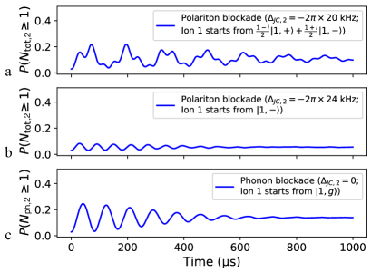
Figure 4: Numerically calculated results for (a),(b) polariton and (c) phonon populations in the respective excited states at Ion 2, plotted against elapsed time. In (a) and (b), the total population in the states with polariton number of one or greater, $P({N}_{\mathrm{tot},2}\geq 1)$, for $\Delta_{\mathrm{JC},2}=-2\pi\times 20$ kHz and $-2\pi\times 24$ kHz, respectively and the initial state at Ion 1 of $(\ket{0,e}-i\ket{1,g})/\sqrt{2}=\frac{1-i}{2}\ket{1,{+}}+\frac{1+i}{2}\ket{1,{-}}$ and $\ket{1,-}$ is plotted. In (c), the total population in the states with the phonon number of one or greater, $P({N}_{\mathrm{ph},2}\geq 1)$, is plotted

We have found that the amount of leakage as given in the last paragraph can be suppressed by choosing the appropriate conditions, that is, those for the detuning at Ion 2 and the initial state at Ion 1. Figure 4(b) displays a result for such a case. Here, the detuning $\Delta_{\mathrm{JC,2}}$ is set to be $-2\pi\times 24$ kHz, and $\ket{1,{-}}$ is chosen as the initial state. We find lower leakage for the Ion 1 initial state of $\ket{1,{-}}$, compared with $\ket{1,{+}}$ (or any superpositions of those), around this value of the detuning. The amount of leakage at this point is obtained to be 0.0549. At this detuning, the eigenenergy of $\ket{1,{-}}$ at Ion 1, which is calculated to be $-2\pi\times 11.8$ kHz, is different from the eigenenergies for Ion 2 ($-2\pi\times 28.8$ kHz and $2\pi\times 4.8$ kHz, represented by red circles in Fig. 1); that is, there exist finite energy gaps between the eigenenergies at Ion 1 and Ion 2. This condition is not satisfied to the same extent for detunings in other regions, and either of the two eigenenergies at Ion 2 become closer to that of $\ket{1,{-}}$ at Ion 1 (see also Table 1 for the relevant eigenenergies as well as the amount of leakage against various negative values for the detuning). If the detuning is decreased from $-2\pi\times 24$ kHz, we observe that the leakage increases. We speculate that the energy gaps, as introduced above, can approximately explain the behavior that the leakage takes the minimum value at around $-2\pi\times 24$ kHz. We can confirm from Table 1 that the smaller of the two relevant energy gaps, $E_{1,-,1}-E_{1,-,2}$ and $E_{1,+,2}-E_{1,-,1}$ ($E_{1,\pm,i}$ represents the eigenenergy of $\ket{1,\pm}$ at the $i$th ion), takes the largest value ($2\pi\times 16.6$ kHz) at $\Delta_{\mathrm{JC,2}}=-2\pi\times 24$ kHz. We should note that the eigenenergies shown in Fig. 1 and Table 1 incorporate only local JC interactions and not the hopping term, and hence, the above-mentioned explanation holds only approximately.

Table 1: Eigenenergies, their differences and the amount of leakage against the negative values of the detuning $\Delta_{\mathrm{JC},2}$. The values for the detuning and the eigenenergies have units of $2\pi\times$kHz. It is assumed that $E_{1,-,1}\sim-2\pi\times 11.8$ kHz

$\Delta_{\mathrm{JC},2}$	$E_{1,-,2}$	$E_{1,+,2}$	$E_{1,-,1}-E_{1,-,2}$	$E_{1,+,2}-E_{1,-,1}$	$\langle{}P({N}_{\mathrm{tot},2}\geq 1)\rangle$
$-$500	$-$500.3	0.3	488.5	12.0	0.0805
$-$100	$-$101.4	1.4	89.6	13.1	0.0718
$-$50	$-$52.6	2.6	40.9	14.4	0.0631
$-$30	$-$34.1	4.1	22.3	15.8	0.0563
$-$28	$-$32.3	4.3	20.5	16.0	0.0557
$-$26	$-$30.5	4.5	18.8	16.3	0.0551
$-$24	$-$28.8	4.8	17.0	16.6	0.0549
$-$22	$-$27.1	5.1	15.3	16.9	0.0551
$-$20	$-$25.4	5.4	13.7	17.2	0.0560
$-$15	$-$21.4	6.4	9.7	18.2	0.0628
$-$10	$-$17.8	7.8	6.0	19.5	0.1040

Table 2: Eigenenergies, their differences and the amount of leakage against the positive values of the detuning $\Delta_{\mathrm{JC},2}$. The values for the detuning and the eigenenergies have units of $2\pi\times$kHz It is assumed that $E_{1,+,1}\sim 2\pi\times 11.8$ kHz

$\Delta_{\mathrm{JC},2}$	$E_{1,-,2}$	$E_{1,+,2}$	$E_{1,+,1}-E_{1,-,2}$	$E_{1,+,2}-E_{1,+,1}$	$\langle{}P({N}_{\mathrm{tot},2}\geq 1)\rangle$
10	$-$7.8	17.8	19.5	6.0	0.1038
15	$-$6.4	21.4	18.2	9.7	0.0627
20	$-$5.4	25.4	17.2	13.7	0.0558
22	$-$5.1	27.1	16.9	15.3	0.0550
24	$-$4.8	28.8	16.6	17.0	0.0545
26	$-$4.5	30.5	16.3	18.8	0.0547
28	$-$4.3	32.3	16.0	20.5	0.0553
30	$-$4.1	34.1	15.8	22.3	0.0560
50	$-$2.6	52.6	14.4	40.9	0.0626
100	$-$1.4	101.4	13.1	89.6	0.0712
500	$-$0.3	500.3	12.0	488.5	0.0799

The amount of leakage for the positive values of the detuning $\Delta_{\mathrm{JC,2}}$ along with the relevant eigenenergies are summarized in Table 2. For positive detuning, the initial state of $\ket{1,+}$ at Ion 1 gives a lower leakage to Ion 1, and hence, only the results in this case are shown in the table and the case of $\ket{1,-}$ is omitted. We confirm that the dependence of the leakage against the detuning shows an approximately symmetric behavior when compared with the case of negative detuning (Table 1). Qualitatively, this can be well understood from the symmetry of the eigenenergy values, as is seen in Fig. 1, Table 1 and Table 2.

5.2 Comparison with phonon blockade

We also estimate the leakage in the case of phonon hopping, as studied in Debnath et al. (2018), for comparison with the polariton case studied here. Formally, the phonon hopping case corresponds to the assumption that $\Delta_{\mathrm{JC,2}}=0$ and $\ket{1,g}$ is used for the initial state at Ion 1. We use the same value of the JC coupling constant at Ion 2 as before, $2g_{2}=2\pi\times 24$ kHz. The numerically calculated result for the time dependence of $P({N}_{\mathrm{ph},2}\geq 1)$ in this case is shown in Fig. 4(c), where ${N}_{\mathrm{ph},2}$ is the quantum number for $\hat{N}_{\mathrm{ph},2}\equiv\hat{a}_{2}^{\dagger}\hat{a}_{2}$ representing the phonon number at Ion 2. The average of $P({N}_{\mathrm{ph},2}\geq 1)$ over the displayed time range is obtained to be 0.139.

So far, we have assumed that the phonon system has a finite thermal distribution (we have assumed $\langle{n}_{y}\rangle=0.03$ in the numerical calculations). To precisely compare the cases for polaritons and phonons, we should use the amounts of leakage in the cases without the thermal distribution. We have also performed numerical calculations for this case, and the results are as follows: for a polariton blockade with $\Delta_{\mathrm{JC,2}}=-2\pi\times 24$ kHz and $\ket{1,-}$ as the initial state at Ion 1, the amount of leakage is 0.0297, while for a phonon blockade it is 0.1144. Therefore, it is expected that, for a polariton blockade based on the scheme presented in this work, the amount of leakage is smaller than the case of phonon hopping by approximately four times, assuming the same intensity of the optical beam at Ion 2.

6 Conclusions

In conclusion, we have demonstrated the site-dependent control of polaritons in the Jaynes–Cummings–Hubbard (JCH) model with trapped ions. We have presented experimental results on blocking the hopping of a polariton initialized in an ion site to an adjacent site, by shifting the frequency of the optical beam illuminating the latter. We have also performed numerical calculations to estimate the leakage to the adjacent ion site. Based on the calculated results, we have found that the gaps between the relevant eigenenergies at both ion sites may partly explain the dependence of the amount of leakage on the frequency shift. The scheme presented here can be applied to various studies on polariton systems in the JCH model, including quasi-static as well as nonequilibrium behaviors.

Acknowledgments

This article was supported by MEXT Quantum Leap Flagship Program (MEXT Q-LEAP) Grant Number JPMXS0118067477.

Declarations

Conflict of interest The authors declare no conflicts of interest.

References

- Feynman (1982) R. P. Feynman, Int. J. Theor. Phys. 21, 467 (1982).
- Blatt and Roos (2012) R. Blatt and C. F. Roos, Nat. Phys. 8, 277 (2012).
- Cirac and Zoller (2012) J. I. Cirac and P. Zoller, Nature Phys. 8, 264 (2012).
- Daley et al. (2022) A. J. Daley, I. Bloch, C. Kokail, S. Flannigan, N. Pearson, M. Troyer, and P. Zoller, Nature 607, 667 (2022).
- Greentree et al. (2006) A. D. Greentree, C. Tahan, J. H. Cole, and L. C. L. Hollenberg, Nat. Phys. 2, 856 (2006).
- Hartmann et al. (2006) M. J. Hartmann, F. Brandao, and M. B. Pleino, Nat. Phys. 2, 849 (2006).
- Angelakis et al. (2007) D. G. Angelakis, M. F. Santos, and S. Bose, Phys. Rev. A 76, 031805 (2007).
- Ivanov et al. (2009) P. A. Ivanov, S. S. Ivanov, N. V. Vitanov, A. Mering, M. Fleischhauer, and K. Singer, Phys. Rev. A 80, 060301(R) (2009).
- Jaynes and Cummings (1963) E. T. Jaynes and F. W. Cummings, Proc. IEEE 51, 89 (1963).
- Hoffman et al. (2011) A. J. Hoffman, S. J. Srinivasan, S. Schmidt, L. Spietz, J. Aumentado, H. E. Tureci, and A. A. Houck, Phys. Rev. Lett. 107, 053602 (2011).
- Raftery et al. (2014) J. Raftery, D. Sadri, S. Schmidt, H. E. Tureci, and A. A. Houck, Phys. Rev. X 4, 031043 (2014).
- Fitzpatrick et al. (2017) M. Fitzpatrick, N. M. Sundaresan, A. C. Y. Li, J. Koch, and A. A. Houck, Phys. Rev. X 7, 011016 (2017).
- Toyoda et al. (2013) K. Toyoda, Y. Matsuno, A. Noguchi, S. Haze, and S. Urabe, Phys. Rev. Lett. 111, 160501 (2013).
- Debnath et al. (2018) S. Debnath, N. M. Linke, S.-T. Wang, C. Figgatt, K. A. Landsman, L.-M. Duan, and C. Monroe, Phys. Rev. Lett. 120, 073001 (2018).
- Li et al. (2022) B. W. Li, Q. X. Mei, Y. K. Wu, M. L. Cai, Y. Wang, L. Yao, Z. C. Zhou, and L. M. Duan, Phys. Rev. Lett. 129, 140501 (2022).
- Islam et al. (2011) R. Islam, E. E. Edwards, K. Kim, S. Korenblit, C. Noh, H. Carmichael, G. D. Lin, L.-M. Duan, C. C. Joseph Wang, J. K. Freericks, and C. Monroe, Nat. Commun. 2, 377 (2011).
- Wong and Law (2011) M. T. C. Wong and C. K. Law, Phys. Rev. A 83, 055802 (2011).
- Nissen et al. (2012) F. Nissen, S. Schmidt, M. Biondi, G. Blatter, H. E. Tureci, and J. Keeling, Phys. Rev. Lett. 108, 233603 (2012).
- Li et al. (2021) Q. Li, J. L. Ma, T. Huang, L. Tan, H. Q. Gu, and W. M. Liu, EPL 134, 20007 (2021).
- Cohen-Tannoudji (2005) C. Cohen-Tannoudji, Atoms In Electromagnetic Fields (World Scientific, Singapore, 2005).
- Ohira et al. (2021) R. Ohira, S. Kume, H. Takahashi, and K. Toyoda, Quantum Sci. Technol. 6, 024015 (2021).
- Porras and Cirac (2004) D. Porras and J. I. Cirac, Phys. Rev. Lett. 93, 263602 (2004).
- Haze et al. (2012) S. Haze, Y. Tateishi, A. Noguchi, K. Toyoda, and S. Urabe, Phys. Rev. A 85, 031401(R) (2012).
- Tamura et al. (2020) M. Tamura, T. Mukaiyama, and K. Toyoda, Phys. Rev. Lett. 124, 200501 (2020).
- Zhu et al. (2006) S.-L. Zhu, C. Monroe, and L. M. Duan, Phys. Rev. Lett. 97, 050505 (2006).
- Donley et al. (2005) E. A. Donley, T. P. Heavner, F. Levi, M. O. Tataw, and S. R. Jefferts, Rev. Sci. Instrum. 76, 063112 (2005).
- Ohira et al. (2022) R. Ohira, S. Kume, and K. Toyoda, Phys. Rev. A 106, 042603 (2022).
- Muralidharan et al. (2021) S. Muralidharan, R. Ohira, S. Kume, and K. Toyoda, Phys. Rev. A 104, 062410 (2021).