More on Half-Wormholes and Ensemble Average

Abstract

We continue our study Peng:2022pfa about the half-wormhole proposal. By generalizing the original proposal of half-wormhole we propose a new way to detect half-wormholes. The crucial idea is to decompose the observables into self-averaged sector and non-self-averaged sectors. We find the contributions from different sectors have interesting statistics in the semi-classical limit. In particular, dominant sectors tend to condense and the condensation explains the emergence of half-wormholes and we expect that the appearance of condensation is a signal of possible bulk description. We also initiate the study of multi-linked-half-wormholes using our approach.

1 Introduction

Recent progress in quantum gravity and black hole physics impresses on the fact that wormholes play important roles. Many evidences suggest an appealing conjectural duality between a bulk gravitation theory and an ensemble theory on the boundary Saad:2019lba ; Stanford:2019vob ; Iliesiu:2019lfc ; Kapec:2019ecr ; Maxfield:2020ale ; Witten:2020wvy ; Arefeva:2019buu ; Betzios:2020nry ; Anninos:2020ccj ; Berkooz:2020uly ; Mertens:2020hbs ; Turiaci:2020fjj ; Anninos:2020geh ; Gao:2021uro ; Godet:2021cdl ; Johnson:2021owr ; Blommaert:2021etf ; Okuyama:2019xbv ; Forste:2021roo ; Maloney:2020nni ; Afkhami-Jeddi:2020ezh ; Cotler:2020ugk ; Benjamin:2021wzr ; Perez:2020klz ; Cotler:2020hgz ; Ashwinkumar:2021kav ; Afkhami-Jeddi:2021qkf ; Collier:2021rsn ; Benjamin:2021ygh ; Dong:2021wot ; Dymarsky:2020pzc ; Meruliya:2021utr ; Bousso:2020kmy ; Janssen:2021stl ; Cotler:2021cqa ; Marolf:2020xie ; Balasubramanian:2020jhl ; Gardiner:2020vjp ; Belin:2020hea ; Belin:2020jxr ; Altland:2021rqn ; Belin:2021ibv ; Peng:2021vhs ; Banerjee:2022pmw ; Johnson:2022wsr ; Collier:2022emf ; Chandra:2022bqq ; Schlenker:2022dyo ; Kruthoff:2022voq ; Kar:2022vqy ; Cotler:2022rud . For example the seminal work Saad:2019lba shows that Jackiw-Teitelboim (JT) gravity is equivalent to a random matrix theory. On the other hand this new conjectural duality is not compatible with our general belief about the AdS/CFT correspondence. A sharp tension is the puzzle of factorization Witten:1999xp ; Maldacena:2004rf . In Saad:2021uzi , this puzzle is studied within a toy model introduced in Marolf:2020xie , where they find that (approximate) factorization can be restored if other saddles which are called half-wormholes are included. Motived by this idea, in Saad:2021rcu a half-wormhole saddle is proposed in a 0-dimensional (0d) SYK model , followed by further analyses in different models Mukhametzhanov:2021nea ; Garcia-Garcia:2021squ ; Choudhury:2021nal ; Mukhametzhanov:2021hdi ; Okuyama:2021eju ; Goto:2021mbt ; Blommaert:2021fob ; Goto:2021wfs . In our previous works Peng:2021vhs ; Peng:2022pfa , we pointed out the connection between the gravity computation in Saad:2021uzi and the field theory computation in Saad:2021rcu and tested the half-wormhole proposal in various models. The main difficulty of this proposal is the construction of the half-wormhole saddles. Further more the ansatz proposed in Saad:2021rcu ; Mukhametzhanov:2021hdi seems to rely on the fact the ensemble is Gaussian with zero mean value. As a result, the 0d SYK model only has non-trivial cylinder wormhole amplitude. However for a generic gravity theory for example the JT gravity, disk and all kinds of wormhole amplitudes should exist. In our previous work Peng:2022pfa , we find even turning on disk amplitude in 0d SYK model will change the half-wormhole ansatz dramatically.

In this work, we generalize the idea of Saad:2021uzi and propose a method of searching for half-wormhole saddles. In our proposal, the connection between Saad:2021uzi and Saad:2021rcu will manifest. One notable benefit of our approach is that it does not depend on the trick of introducing a resolution identity used in Saad:2021rcu , the collective variables emerge automatically. More importantly our proposal can be straightforwardly generalized to non-Gaussian ensemble theories.

2 Gaussian distribution or the CGS model

In Saad:2021uzi , the main model is the Coleman and Giddings-Strominger (CGS) model. The CGS model is a toy model of describing spacetime wormholes and it is more suggestive to obtain it from the Marolf-Maxfield (MM) model Marolf:2020xie by restricting the sum over topologies to only include the disk and the cylinder Saad:2021uzi .

Let the amplitudes of the disk and cylinder be $\mu$ and $t^{2}$, i.e.

$$\langle\hat{Z}\rangle=\mu,\quad\langle\hat{Z}^{2}\rangle-\langle\hat{Z}\rangle^{2}=t^{2},$$ (1)

where $|\rangle=|\text{HH}\rangle$ denotes the no-boundary (Hartle-Hawking) state and $\hat{Z}$ denotes the boundary creation operator thus $\langle\hat{Z}^{n}\rangle$ computes the Euclidean path integral over all manifolds with $n$ boundaries. For CGS model the gravity amplitude or the “correlation function of the partition function” $\langle\hat{Z}^{n}\rangle$ is a polynomial of $\mu$ and $t^{2}$ and in particular its generating function is simply

$$\langle e^{u\hat{Z}}\rangle=\exp\left({u\mu+\frac{u^{2}t^{2}}{2}}\right).$$ (2)

Thus we can identify $\hat{Z}$ as a Gaussian random variable $Z$ such that the gravity amplitude $\langle f(\hat{Z})\rangle$ can be computed as the ensemble average $\mathbb{E}(f(Z))\equiv\langle f(Z)\rangle$. This equivalence is a baby version of gravity/ensemble duality.

The crucial idea of Saad:2021uzi is that the correlation functions of partition function does not factorize in general but they factorize between $\alpha$–states which are the eigenstates of $\hat{Z}$

$$\langle\alpha|\hat{Z}^{2}|\alpha\rangle=\langle\alpha|\hat{Z}|\alpha\rangle^{2}=Z_{\alpha}^{2}.$$ (3)

The $\alpha$-state is also created by a generation operator acting on $|\text{HH}\rangle$

$$|\alpha\rangle=\psi_{\alpha}|\text{HH}\rangle.$$ (4)

Note that $\psi$ can be expressed in terms of $\hat{Z}$ in a very complicated way so $\psi$ commutes with $\hat{Z}$. Then (3) can be rewritten in a very suggestive way

$$Z_{\alpha}^{2}=\langle\psi_{\alpha}^{2}\hat{Z}^{2}\rangle=\langle\hat{Z}^{2}\rangle+\langle\psi_{\alpha}^{2}\hat{Z}^{2}\rangle_{c},$$ (5)

where we have assumed that $\alpha$-state is normalized $\langle\psi_{\alpha}^{2}\rangle=1$. This rewriting is interesting because it separates out the self-averaged part $\langle\hat{Z}^{2}\rangle$ and non-self-averaged part $\langle\psi_{\alpha}^{2}\hat{Z}^{2}\rangle_{c}$. In CGS model, since the eigenvalue of $\hat{Z}$ is continuous and supported on $\mathbb{R}$ so that we can express $\psi_{\alpha}$ in terms of $\hat{Z}$ schematically as

$$\psi_{\alpha}=\delta(\hat{Z}-Z_{\alpha})=\int\frac{\operatorname{d}k}{2\pi}e^{\text{i}k(\hat{Z}-Z_{\alpha})},$$ (6)

thus

$$\langle Z^{2}\psi_{\alpha}\rangle=\int\frac{\operatorname{d}k\,e^{-\text{i}kZ_{\alpha}}}{2\pi}\langle Z^{2}e^{\text{i}kZ}\rangle\,$$ (7)

$$\rightarrow Z_{\alpha}^{2}=\int\frac{\operatorname{d}k\,e^{-\text{i}kZ_{\alpha}}}{2\pi}\frac{\langle Z^{2}e^{\text{i}kZ}\rangle}{\langle\psi_{\alpha}\rangle}.$$ (8)

Noting that $\langle\psi_{\alpha}\rangle=P(Z_{\alpha})$, where $P(Z)$ is the PDF of $Z$, we find that (8) coincides with the trick used in Peng:2022pfa and Mukhametzhanov:2021hdi of rewriting $Z_{\alpha}^{n}$ as a formal average

$$Z_{\alpha}^{n}=\int\operatorname{d}Z\delta(Z-Z_{\alpha})\frac{Z^{n}P(Z)}{P(Z_{\alpha})}=\int\frac{\operatorname{d}k}{2\pi}\frac{e^{-\text{i}kZ_{\alpha}}}{P(Z_{\alpha})}\langle Z^{n}e^{\text{i}kZ}\rangle.$$ (9)

From which we can derived some useful approximation formula $Z_{\alpha}^{n}\approx\langle Z_{\alpha}^{n}\rangle+\Phi$, where $\langle Z_{\alpha}^{n}\rangle$ and $\Phi$ are respectively recognized as the wormhole and half-wormhole contributions as shown in Peng:2022pfa ; Mukhametzhanov:2021hdi . So we can think of this trick as a refinement of the factorization proposal of Saad:2021uzi . We will elaborate this below.

2.1 Half-Wormhole in CGS-like model

In the CGS model, because $Z$ satisfies the Gaussian distribution there is a more concrete expression for the half wormhole saddle as shown in Saad:2021uzi . The key point is the fact that when $Z$ is Gaussian, it can be thought of as the position operator of a simple harmonic oscillator so there exists a natural orthogonal basis, the number basis $\{n\}$ which is called the $n$-baby universe basis in the context of the gravity model. If we insert the complete basis $\sum_{i}|i\rangle\langle i|$ into (9) we can get

$$Z_{\alpha}^{n} = \int\operatorname{d}Z\delta(Z-Z_{\alpha})\frac{Z^{n}P(Z)}{P(Z_{\alpha})}=\int\frac{\operatorname{d}k}{2\pi}\frac{e^{-\text{i}kZ_{\alpha}}}{P(Z_{\alpha})}\langle Z^{n}e^{\text{i}kZ}\rangle$$ (10)

$$= \int\frac{\operatorname{d}k}{2\pi}\frac{e^{-\text{i}kZ_{\alpha}}}{P(Z_{\alpha})}\sum_{i=0}^{n}\langle Z^{n}|i\rangle\langle i|e^{\text{i}kZ}\rangle$$ (11)

$$= \int\frac{\operatorname{d}k}{2\pi}\frac{e^{-\text{i}kZ_{\alpha}}}{P(Z_{\alpha})}\sum_{i=0}^{n}{n\choose i}\langle Z^{n-i}\rangle\langle Z^{i}|i\rangle\langle i|e^{\text{i}kZ}\rangle$$ (12)

$$= \int\frac{\operatorname{d}k}{2\pi}\frac{e^{-\text{i}kZ_{\alpha}}}{P(Z_{\alpha})}\sum_{i=0}^{n}{n\choose i}\langle Z^{n-i}\rangle\sqrt{i!}t^{i}\langle i|e^{\text{i}kZ}\rangle$$ (13)

$$= \int\frac{\operatorname{d}k}{2\pi}\frac{e^{-\text{i}kZ_{\alpha}}}{P(Z_{\alpha})}\sum_{i=0}^{n}{n\choose i}\langle Z^{i}\rangle\langle(at)^{n-i}e^{\text{i}kZ}\rangle\equiv\sum_{i=0}^{n}{n\choose i}\mu_{i}\theta^{(n-i)},$$ (14)

where

$$\theta^{(n-i)}=\int\frac{\operatorname{d}k}{2\pi}\frac{e^{-\text{i}kZ_{\alpha}}}{P(Z_{\alpha})}\langle e^{\text{i}kZ}\rangle\frac{\langle(at)^{n-i}e^{\text{i}kZ}\rangle}{\langle e^{\text{i}kZ}\rangle},\quad\frac{\langle(at)^{n-i}e^{\text{i}kZ}\rangle}{\langle e^{\text{i}kZ}\rangle}\equiv\phi^{c}_{n-i}.$$ (15)

Note that

$$\frac{\langle(at)^{n-i}e^{\text{i}kZ}\rangle}{\langle e^{\text{i}kZ}\rangle}\equiv\phi^{c}_{n-i}=(\text{i}kt^{2})^{n-i}=(\phi^{c}_{1})^{n-i},$$ (16)

$$\theta^{(i)}=\int\frac{\operatorname{d}k}{2\pi}\frac{e^{-\text{i}kZ_{\alpha}}}{P(Z_{\alpha})}\langle e^{\text{i}kZ}\rangle(\text{i}kt^{2})^{i}=\frac{(-t^{2}\partial_{Z_{\alpha}})^{i}P(Z_{\alpha})}{P(Z_{\alpha})},$$ (17)

then (14) coincides with results in Peng:2022pfa . So we confirm the result that within the Gaussian approximation (only keep the first two cumulants), $Z^{n}_{\alpha}$ can be decomposed as (14) and it suggests that $\theta_{i}$’s are the convenient building blocks of possible half-wormhole saddles. Some examples of the decomposition (14) are

$$Z_{\alpha}^{1}=\theta^{(1)}+\langle Z\rangle,$$ (18)

$$Z_{\alpha}^{2}=\theta^{(2)}+2\langle Z\rangle\theta^{(1)}+\langle Z^{2}\rangle,$$ (19)

$$Z_{\alpha}^{3}=\theta^{(3)}+3\langle Z\rangle\theta^{(2)}+3\langle Z^{2}\rangle\theta^{(1)}+\langle Z^{3}\rangle,$$ (20)

$$Z_{\alpha}^{4}=\theta^{(4)}+4\langle Z\rangle\theta^{(3)}+6\langle Z^{2}\rangle\theta^{(2)}+4\langle Z^{3}\rangle\theta^{(1)}+\langle Z^{4}\rangle,$$ (21)

with

$$\theta^{(1)}=-\mu+Z_{\alpha},\quad\theta^{(2)}=(\mu-Z_{\alpha})^{2}-t^{2}={\theta^{(1)}}^{2}-t^{2},$$ (22)

$$\theta^{(3)}=-(\mu-Z_{\alpha})^{3}+3(\mu-Z_{\alpha})t^{2}={\theta^{(1)}}^{3}-3t^{2}\theta^{(1)},$$ (23)

$$\theta^{(4)}=3t^{4}-6t^{2}(\mu-Z_{\alpha})^{2}+(\mu-Z_{\alpha})^{4}={\theta^{(1)}}^{4}-6t^{2}{\theta^{(1)}}^{2}+3t^{4}.$$ (24)

In general we have

$$\theta^{(i)}=\int\frac{\operatorname{d}k}{2\pi}\frac{e^{-\text{i}kZ_{\alpha}}}{P(Z_{\alpha})}\langle e^{\text{i}kZ}\rangle(\text{i}kt^{2})^{i} = \int\frac{\operatorname{d}k}{\sqrt{2\pi/t^{2}}}e^{-\frac{(k-(\text{i}(\mu-Z_{\alpha})/t^{2}))^{2}}{2/t^{2}}}(\text{i}kt^{2})^{i},$$ (25)

so $\theta^{(i)}/(\text{i}t^{2})^{i}$ is the $i$-th moment of “Gaussian distribution” $\mathcal{N}(\text{i}(\mu-Z_{\alpha})/t^{2},1/t^{2})$ and the generating function is

$$\langle e^{uk}\rangle_{k}=e^{\frac{\text{i}u(\mu-Z_{\alpha})}{t^{2}}+\frac{u^{2}}{2t^{2}}}.$$ (26)

Considering the following ensemble average

$$\Big{\langle}\langle e^{u_{1}k_{1}}\rangle_{k_{1}}\langle e^{u_{2}k_{2}}\rangle_{k_{2}}\Big{\rangle}_{Z_{\alpha}}=e^{-\frac{u_{1}u_{2}}{t^{2}}},$$ (27)

and expanding both sides into Taylor series of $u_{1}$ and $u_{2}$ one can find

$$\langle\theta^{(i)}\theta^{(j)}\rangle_{Z_{\alpha}}=i!t^{2i}\delta_{ij}.$$ (28)

Due to this orthogonal condition we can directly tell which sector in the decomposition of $Z_{\alpha}^{n}$ is dominant by computing $\langle Z^{n}_{\alpha}Z^{n}_{\alpha}\rangle$

$$Z_{\alpha}^{n}=\sum_{i}c_{i}\theta^{(i)},\quad\langle Z_{\alpha}^{n}Z_{\alpha}^{n}\rangle=\sum_{i}c_{i}^{2}i!t^{2i}.$$ (29)

In CGS model, since there is only a single random variable $Z$ so it does not admit any approximation related to large $N$ or small $G_{N}$. Therefore the wormhole or half-wormhole are not true saddles in the usual sense. To breath life into them we should consider a model with a large number $N$ of random variables such as random matrix theory or SYK model which can be described by certain semi-classical collective variables like the $G,\Sigma$ in SYK, which potentially have a dual gravity description. However we find that it is illustrative to firstly apply the factorization proposal to some simple statistical models as we did in Peng:2022pfa .

2.2 Statistical model

Let us consider a function $Y(X_{i})$ of a large number $N$ independent random variables $X_{i}$. Assuming that $X_{i}$’s are drawn from the Gaussian distribution then we have the decomposition

$$Y^{n} = \frac{1}{(2\pi)^{N}}\int\prod_{i}\left(\operatorname{d}k_{i}\frac{e^{-\text{i}k_{i}X_{i}}}{P(X_{i})}\right)\langle e^{\text{i}\sum_{i}k_{i}x_{i}}\rangle\sum_{n_{1},\dots,n_{N}}\langle Y^{n}|n_{1},\dots,n_{N}\rangle\frac{\langle n_{1},\dots,n_{N}|e^{\text{i}\sum_{i}k_{i}x_{i}}\rangle}{\langle e^{\text{i}\sum_{i}k_{i}x_{i}}\rangle}$$ (30)

$$= \sum_{k=\sum_{i}n_{i}}\Gamma_{k},$$

where $\Gamma_{k}$ denotes different sectors, in particular $\Gamma_{0}=\langle Y^{n}\rangle$. This kind of model can be also thought of as the CGS model with species Saad:2021uzi .

2.2.1 Simple observables

The simplest operator is

$$Y=\sum_{i=1}^{N}X_{i}.$$ (31)

Apparently for $n=1$ there are only two sectors

$$Y=\sum_{i=1}^{N}\mu+\sum_{i=1}^{N}\theta_{i}^{(1)}=\Theta_{0}+\Theta_{1},\quad\langle\Theta_{0}^{2}\rangle=N^{2}\mu^{2},\quad\langle\Theta_{1}^{2}\rangle=Nt^{2},$$ (32)

and for $n=2$ there are three sectors

$$Y^{2}=\Phi_{0}+\Phi_{1}+\Phi_{2},$$ (33)

$$\Phi_{0}=\langle Y^{2}\rangle,\quad\Phi_{1}=2N\mu\sum_{i}\theta_{i}^{(1)},$$ (34)

$$\Phi_{2}=\sum_{ij}\left(\theta_{i}^{(1)}\theta_{j}^{(1)}+\delta_{ij}(\theta_{i}^{(2)}-{\theta_{i}^{(1)}}^{2})\right)=\sum_{ij}\left(\theta_{i}^{(1)}\theta_{j}^{(1)}-\delta_{ij}t^{2}\right).$$ (35)

In general the parameters $\mu$ and $t^{2}$ are $N$ independent therefore $Y^{n}$ is self-averaged $Y^{n}\approx\langle Y^{n}\rangle$ in the large $N$ limit. This is also true even $X_{i}$ are not Gaussian because of the central limit theorem. But we also know in the literature that in order to have well-defined semi-classical approximation, the parameters $\mu$ and $t^{2}$ should depend on $N$ in a certain way like in SYK model. Interestingly in this case if $t^{2}\sim\mu^{2}N$, the self-averaged part and non-self-averaged part are comparable and we should keep them both. This is exactly what we have encountered in the 0-SYK model. But a crucial difference is that for this simple choice of observables, all the non-self-averaged sectors are also comparable so it is not fair to call any of them the half-wormhole saddle and to restore factorization we have to include all the non-self-averaged sectors. The extremal case is $t^{2}>>\mu^{2}N$. In this limit we find that the sector with highest level dominates. For example,

$$Y\approx\Theta_{1},\quad Y^{2}\approx\langle Y^{2}\rangle+\Phi_{2},$$ (36)

$$\langle\Theta_{1}^{2}\rangle\approx\langle Y^{2}\rangle,\quad\langle\Phi_{2}^{2}\rangle\approx 2\langle Y^{2}\rangle^{2},$$ (37)

then it is reasonable to identify $\Theta_{1}$ with half-wormhole and identify $\Phi_{2}$ with the 2-linked half-wormhole. Similarly we can introduce $n$-linked half-wormholes. For example, in this extremal case, we can approximate $Y^{3}$ with

$$Y^{3}\approx 3\langle Y^{2}\rangle\Theta_{1}+\Lambda_{3},$$ (38)

$$\Lambda_{3}=\sum_{i\neq j\neq k}\left(\theta_{i}^{(1)}\theta_{j}^{(1)}\theta_{k}^{(1)}\right)+3\sum_{i\neq j}\theta_{i}^{(2)}\theta_{j}^{(1)}+\sum_{i}\theta_{i}^{(3)},$$ (39)

$$\quad~{}=\sum_{i,j,k}\left(\theta_{i}^{(1)}\theta_{j}^{(1)}\theta_{k}^{(1)}\right)-3t^{2}N\sum_{i}\theta_{i}^{(1)},$$ (40)

where the sector $\Lambda_{3}$ should describe the 3-linked half-wormhole. We will consider a similar construction in the 0-SYK model.

2.2.2 Exponential observables

In the Random Matrix Theory or quantum mechanics, the most relevant observable is the exponential operator ${\rm Tr}(e^{\beta H})$ since it relates to the partition function. So it may be interesting to consider a similar exponential operator

$$Y=\sum_{i}e^{\beta X_{i}},$$ (41)

in the toy statistical model. By a Taylor expansion of the exponential operator we find the following decomposition

$$e^{\beta X}=\langle e^{\beta X}\rangle\sum_{k}\frac{\beta^{k}\theta^{(k)}}{k!},\quad\theta^{(0)}\equiv 1,$$ (42)

thus

$$Y=\sum_{k}\Theta_{k},\quad\Theta_{k}=e^{\mu\beta+\frac{\beta^{2}t^{2}}{2}}\sum_{i}\frac{\beta^{k}\theta_{i}^{(k)}}{k!},$$ (43)

$$\langle\Theta_{k}^{2}\rangle=Ne^{2\mu\beta+{t^{2}\beta^{2}}}\frac{(\beta t)^{2k}}{k!},\quad\frac{\langle\Theta_{k}^{2}\rangle}{\langle Y^{2}\rangle}=e^{-t^{2}\beta^{2}}\frac{(\beta t)^{2k}}{k!}\equiv r_{k}.$$ (44)

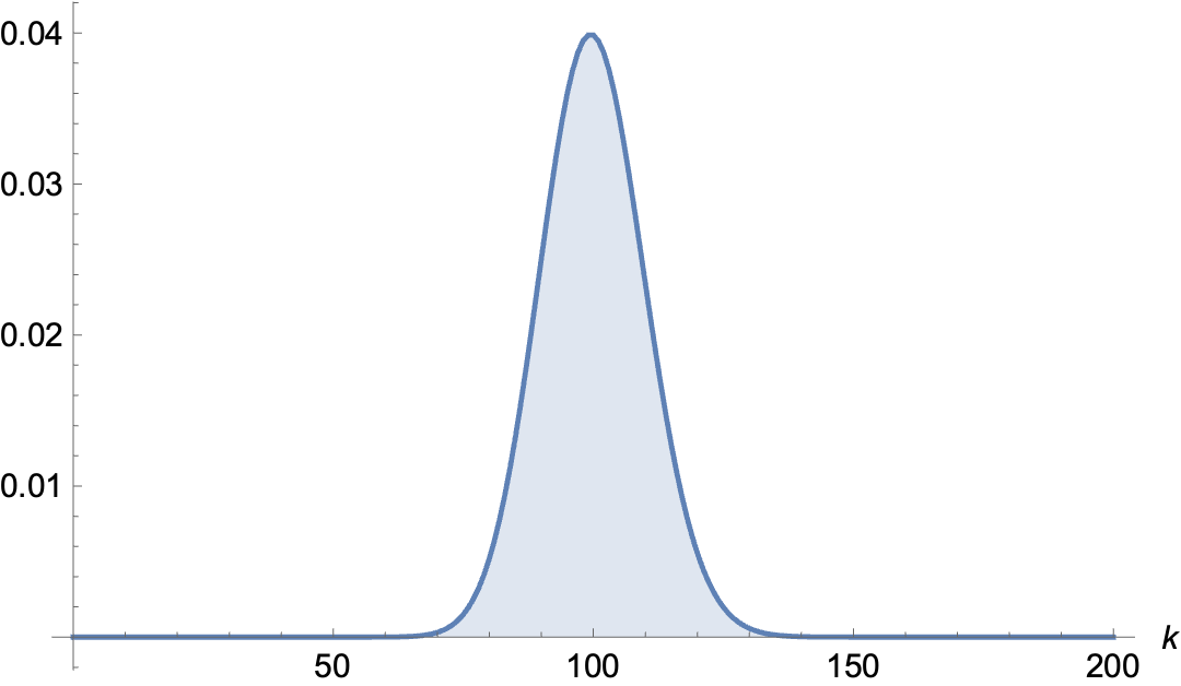
(a)

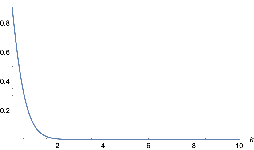
(b)

Figure 1: Poisson distribution (44). (a) Poisson distribution with $\beta^{2}t^{2}=100$, (b) Poisson distribution with $\beta^{2}t^{2}=0.01$.

Interestingly the ratio $r_{k}$ follows the Poisson distribution Pois$(\beta^{2}t^{2})$. When $\beta t<<1$ the dominant sector is $\Theta_{0}$ while for $\beta t>>1$ the Poisson distribution approaches Gaussian distribution $N(\beta^{2}t^{2},\beta^{2}t^{2})$ so we have to include all the sectors in the peak $k\in(\beta^{2}t^{2}-{\beta t},\beta^{2}t^{2}+{\beta t})$ to have a good approximation. We can decompose $Y^{2}$ in a similar way

$$Y^{2}=\sum_{k}\Phi_{k},$$ (45)

$$\Phi_{k}=e^{2\mu\beta+\beta^{2}t^{2}}\beta^{k}\sum_{i\neq j}\sum_{n}\frac{\theta_{i}^{(n)}}{n!}\frac{\theta_{j}^{(k-n)}}{(k-n)!}+e^{2\mu\beta+2\beta^{2}t^{2}}(2\beta)^{k}\sum_{i}\frac{\theta_{i}^{(k)}}{k!},$$ (46)

$$\frac{\langle\Phi_{k}^{2}\rangle}{\langle Y^{4}\rangle}=e^{-2\beta^{2}t^{2}}\frac{(2\beta^{2}t^{2})^{k}}{k!}\frac{2(N-1)+2^{k}e^{2\beta^{2}t^{2}}+4(N-1)e^{\beta^{2}t^{2}}}{2(N-1)+e^{4\beta^{2}t^{2}}+4(N-1)e^{\beta^{2}t^{2}}}.$$ (47)

The behavior is similar. When $\beta t<<1$, the dominant sector is the self-averaged sector $\Phi_{0}$. When $2\beta^{2}t^{2}>\log N$ (47) approaches the Gaussian $N(4\beta^{2}t^{2},4\beta^{2}t^{2})$. On the other hand, when $1<<2\beta^{2}t^{2}<<\log N$ (47) approaches the Gaussian $N(2\beta^{2}t^{2},2\beta^{2}t^{2})$. In the end when $2\beta^{2}t^{2}\sim\log N$, (47) will have two comparable peaks.

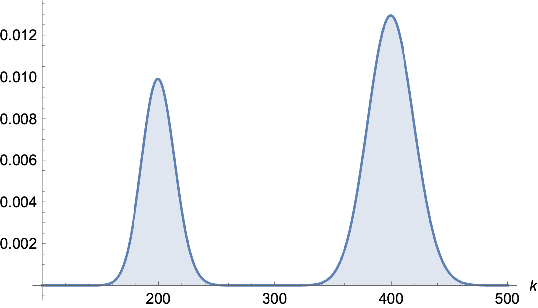
Figure 2: Plot of (47) when they are two comparable peaks. $\log N=298,\quad\beta t=10$.

However the half-wormhole ansatz proposed in Mukhametzhanov:2021hdi ; Peng:2022pfa which can be written as

$$\Phi=\sum_{k=0}^{\infty}\phi_{k},$$ (48)

$$\phi_{k}=\Phi_{k}+(e^{-\beta^{2}t^{2}}-1)e^{2\mu\beta+2\beta^{2}t^{2}}(2\beta)^{k}\sum_{i}\frac{\theta_{i}^{(k)}}{k!},$$ (49)

only works for small value of $\beta t$.

To summarize our proposal, by introducing the basis $\{\theta_{i}\}$ which is the generalization of $n$-baby universe basis Saad:2021uzi we can decompose the observables or partition functions into a single self-averaged sector and many non-self-averaged sectors. These sectors are independent in the sense of (28). The contributions from each sector have interesting statistics: in the large $N$ limit leading contributing sectors may condense to peaks. This condensation is a signal that the observable potentially has a bulk description (or semi-classical description) in the large $N$ limit. If the self-averaged sector survives then it means the observable is approximately self-averaging. The surviving non-self-averaged sectors in the large $N$ limit are naturally interpreted as the ($n$-linked) half-wormholes which are the results of sector condensation. In the extremal case, only one non-self-averaging survives reminiscing the famous Bose-Einstein condensation.

2.3 0-SYK model

In this section we apply our proposal to the 0-SYK model which has the “action”

$$z=\int\operatorname{d}^{N}\psi\exp(\text{i}^{q/2}\sum J_{i_{1}\dots i_{q}}\psi_{i_{1}\dots i_{q}})\,,$$ (50)

where $\psi_{i_{1}\dots i_{q}}=\psi_{a_{1}}\psi_{a_{2}}\dots\psi_{a_{q}}$ and $\psi_{i}$ are Grassmann numbers. The random couplings $J_{i_{1}\dots i_{q}}$ is drawn from a Gaussian distribution

$$\langle J_{i_{1}\dots i_{q}}\rangle=u,\quad\langle J_{i_{1}\dots i_{q}}J_{j_{1}\dots j_{q}}\rangle=t^{2}\delta_{i_{1}j_{1}}\dots\delta_{i_{q}j_{q}},\quad t^{2}=\tau^{2}\frac{(q-1)!}{N^{q-1}}\ ,$$ (51)

where we found in Peng:2022pfa in order to have a semi-classical description $u$ should also have a proper dependence

$$u=(-\text{i})^{q/2}\mu\frac{(q/2-1)!}{2N^{q/2-1}}.$$ (52)

We sometimes use the collective indies $A,B$ to simplify the notation

$$A=\{a_{1}<\dots<a_{q}\}\,,\qquad J_{A}\psi_{A}\equiv J_{a_{1}\dots a_{q}}\psi_{a_{1}\dots a_{q}}\ .$$ (53)

Integrating out the Grassmann numbers directly gives :

$$z=\int\operatorname{d}^{N}\psi\exp(\text{i}^{q/2}J_{A}\psi_{A})=\sum^{\prime}_{A_{1}<\dots<A_{p}}\text{sgn}(A)J_{A_{1}}\dots J_{A_{p}}\,,\quad p=N/q\,,$$ (54)

where the expression (54) is nothing but the hyperpfaffian $\text{Pf}(J)$. According to (30), we can similarly decompose it as

$$z=\sum_{i}\Theta_{i},\quad\Theta_{0}=\langle z\rangle,$$ (55)

$$\Theta_{k}=u^{p-k}\sum^{\prime}_{I_{1}<\dots<I_{p-k}}\text{Pf}(\theta^{(1)(I_{1},\dots,I_{p-k})}_{A}),$$ (56)

where the tensor $\theta^{(1)(I_{1},\dots,I_{p-k})}_{A}$ means that the index $A$ is not in the set $(I_{1},\dots,I_{p-k})$. The expression (56) can be derived by a combinatorial method used in Peng:2022pfa or by using the $G,\Sigma$ trick as follows. First we expand $z$ into series of $\theta^{(1)}$

$$z = \int\operatorname{d}^{N}\psi e^{\text{i}^{q/2}\sum_{A}J_{A}\psi_{A}}=\int\operatorname{d}^{N}\psi e^{\text{i}^{q/2}\sum_{A}u\psi_{A}}e^{\text{i}^{q/2}\sum_{A}\theta_{A}^{(1)}\psi_{A}}$$ (57)

$$= \int\operatorname{d}^{N}\psi\sum_{k=0}\frac{(\text{i}^{q/2}\sum_{A}\theta^{(1)}_{A}\psi_{A})^{k}}{k!}e^{\text{i}^{q/2}u\sum_{A}\psi_{A}},$$ (58)

thus by matching the power of $\theta^{(1)}$ we get a integral expression of $\Theta_{k}$

$$\Theta_{k}=\int\operatorname{d}^{N}\psi\frac{(\text{i}^{q/2}\sum_{A}\theta_{A}^{(1)}\psi_{A})^{k}}{k!}e^{\text{i}^{q/2}u\sum_{A}\psi_{A}}.$$ (59)

Next following Peng:2022pfa we can introduce $G,\Sigma$ variables directly as

$$G = \frac{1}{N}\sum_{i<j}\psi_{i}\psi_{j},$$ (60)

$$z = \int\operatorname{d}^{N}\psi\int_{\mathbb{R}}\operatorname{d}G\int_{\text{i}\mathbb{R}}\frac{\operatorname{d}\Sigma}{2\pi\text{i}/N}e^{u\text{i}^{q/2}\frac{N^{q/2}}{(q/2)!}G^{q/2}}e^{-N\Sigma G}e^{\text{i}^{q/2}\sum_{A}\theta_{A}^{(1)}\psi_{A}}e^{\Sigma\sum_{i<j}\psi_{i}\psi_{j}}$$

$$= \int\operatorname{d}^{N}\psi\int_{\mathbb{R}}\operatorname{d}G\int_{\text{i}\mathbb{R}}\frac{\operatorname{d}\Sigma}{2\pi\text{i}/N}e^{u\text{i}^{q/2}\frac{N^{q/2}}{(q/2)!}G^{q/2}}e^{-N\Sigma G}\sum_{k}\frac{(\text{i}^{q/2}\sum_{A}\theta_{A}^{(1)}\psi_{A})^{k}}{k!}e^{\Sigma\sum_{i<j}\psi_{i}\psi_{j}},$$

and

$$\Theta_{k} = \int\operatorname{d}^{N}\psi\int_{\mathbb{R}}\operatorname{d}G\int_{\text{i}\mathbb{R}}\frac{\operatorname{d}\Sigma}{2\pi\text{i}/N}e^{u\text{i}^{q/2}\frac{N^{q/2}}{(q/2)!}G^{q/2}}e^{-N\Sigma G}\frac{(\text{i}^{q/2}\sum_{A}\theta_{A}^{(1)}\psi_{A})^{k}}{k!}e^{\Sigma\sum_{i<j}\psi_{i}\psi_{j}},$$

$$= \int\operatorname{d}^{N}\psi\int_{\mathbb{R}}\operatorname{d}G\int_{\text{i}\mathbb{R}}\frac{\operatorname{d}\Sigma}{2\pi\text{i}/N}e^{u\text{i}^{q/2}\frac{N^{q/2}}{(q/2)!}G^{q/2}}e^{-N\Sigma G}\frac{(\text{i}^{q/2}\sum_{A}\theta_{A}^{(1)}\psi_{A})^{k}}{k!}\frac{(q/2!)^{p-k}\Sigma^{\frac{N-qk}{2}}(\sum_{A}\psi_{A})^{p-k}}{(N/2-qk/2)!}$$

$$= \int_{\mathbb{R}}\operatorname{d}G\int_{\text{i}\mathbb{R}}\frac{\operatorname{d}\Sigma}{2\pi\text{i}/N}e^{u\text{i}^{q/2}\frac{N^{q/2}}{(q/2)!}G^{q/2}}e^{-N\Sigma G}(\text{i}\Sigma)^{\frac{N-qk}{2}}\frac{(q/2!)^{p-k}(p-k)!}{(N/2-qk/2)!}\times$$

$$\int\operatorname{d}^{N}\psi\sum_{A_{1}<\dots<A_{k}}\theta_{A_{1}}^{(1)}\dots\theta_{A_{k}}^{(1)}\psi_{A_{1}}\dots\psi_{A_{k}}\times\sum_{I_{1}<\dots<I_{p-k}}\psi_{I_{1}}\dots\psi_{I_{p-k}}$$

$$= \int_{\mathbb{R}}\operatorname{d}G\int_{\text{i}\mathbb{R}}\frac{\operatorname{d}\Sigma}{2\pi\text{i}/N}e^{u\text{i}^{q/2}\frac{N^{q/2}}{(q/2)!}G^{q/2}}e^{-N\Sigma G}(\text{i}\Sigma)^{\frac{N-qk}{2}}\frac{(p-k)!(q/2!)^{p-k}}{(N/2-qk/2)!}\times\sum^{\prime}_{I_{1}<\dots<I_{p-k}}\text{PF}(\theta^{(1)(I_{1},\dots,I_{p-k})}_{A}),$$

$$= u^{p-k}\sum^{\prime}_{I_{1}<\dots<I_{p-k}}\text{PF}(\theta^{(1)(I_{1},\dots,I_{p-k})}_{A}),$$ (65)

where the tensor $\theta^{(1)(I_{1},\dots,I_{p-k})}_{A}$ means that the index $A$ is not in the set $(I_{1},\dots,I_{p-k})$. To figure out which one is dominant let us compute

$$\langle z^{2}\rangle=\sum_{i}\langle\Theta_{i}\Theta_{i}\rangle.$$ (66)

The expression of $\langle z^{2}\rangle$ is derived in Peng:2022pfa

$$\langle z^{2}\rangle=\sum_{k=0}^{p}c_{k}m_{p-k}^{2}t^{2k}u^{2p-2k}\equiv\sum_{k}z_{2}^{(k)}\,,$$ (67)

where

$$c_{k}=\frac{1}{k!}{N\choose q}{N-q\choose q}\dots N-(k-1)q\choose q=\frac{N!}{k!(q!)^{k}(N-kq)!}\,,$$ (68)

$$m_{p}=\frac{(pq/2)!}{p!((q/2)!)^{p}}.$$ (69)

By matching the power of $t^{2}$ we can identify

$$z_{2}^{(k)}=\langle\Theta_{k}\Theta_{k}\rangle=c_{k}m_{p-k}^{2}t^{2k}u^{2p-2k}.$$ (70)

The coefficient is very involved so let us first consider some simple cases. If $p=2$, then there are only three sectors

$$z=\langle z\rangle+\Theta_{1}+\Theta_{2},$$ (71)

$$z_{2}^{(0)}=\frac{\left(q!\right)^{2}}{4\left(\frac{q}{2}!\right)^{4}}u^{4},\quad z_{2}^{(1)}=\frac{(2q)!}{\left(q!\right)^{2}}u^{2}t^{2},\quad z_{2}^{(2)}=\frac{(2q)!}{2\left(q!\right)^{2}}t^{4}.$$ (72)

Taking the large $N$ limit, we find

$$z_{2}^{(1)}\sim\sqrt{N}\frac{t^{2}}{u^{2}}z_{2}^{(0)},\quad z_{2}^{(2)}\sim\sqrt{N}\frac{t^{4}}{u^{4}}z_{2}^{(0)},$$ (73)

and

$$\frac{t^{2}}{u^{2}}\approx\frac{1}{N}\frac{\tau^{2}}{4\mu^{2}}\frac{\frac{N}{2}!}{(\frac{N}{4}!)^{2}}\sim\frac{\tau^{2}}{\mu^{2}}\frac{2^{N/2}}{N\sqrt{N}},$$ (74)

which implies that

$$z_{2}^{(1)}\sim\frac{2^{N/2}}{N}z_{2}^{(0)},\quad z_{2}^{(2)}\sim\frac{2^{N}}{N^{2}\sqrt{N}}z_{2}^{(0)}\sim\frac{2^{N/2}}{N\sqrt{N}}z_{2}^{(1)},$$ (75)

so that we have the approximation

$$z\sim\Theta_{2}.$$ (76)

Similarly when $p=3$, we can find

$$z=\langle z\rangle+\Theta_{1}+\Theta_{2}+\Theta_{3},$$ (77)

and

$$z_{2}^{(3)}\sim\frac{t^{2}}{u^{2}}\frac{1}{3}z_{2}^{(2)},\quad z_{2}^{(2)}\sim\frac{t^{2}}{u^{2}}\sqrt{N}z_{2}^{(1)},\quad z_{2}^{(1)}\sim\frac{t^{2}}{u^{2}}\sqrt{N}z_{2}^{(0)},$$ (78)

$$\frac{t^{2}}{u^{2}}\sim\frac{2^{N/3}}{N\sqrt{N}},$$ (79)

thus

$$z\approx\Theta_{3}.$$ (80)

This turns out be general: when $p<<N$ the dominant term is $\Theta_{p}$. Therefore, the self-averaged $\langle z\rangle$ will not survive. This behavior is same as we found in the simple statistical model in the regime when the cylinder amplitude is much larger than the disk amplitude.

On the other hand, if $q<<N$ then

$$\frac{t^{2}}{u^{2}}\sim\frac{\tau^{2}}{\mu^{2}}\sim\frac{1}{N},$$ (81)

the situation is very different. As a simple demonstration let us consider the case of $q=2$

$$z_{2}^{(p)}\sim N^{N/2}\frac{t^{N}}{u^{N}}z_{2}^{(0)}=\frac{1}{N^{N/2}}z_{2}^{(0)},$$ (82)

$$z_{2}^{(1)}\sim N^{2}\frac{t^{2}}{u^{2}}z_{2}^{(0)}=Nz_{2}^{(0)},\quad z_{2}^{(2)}\sim N^{4}\frac{t^{4}}{u^{4}}z_{2}^{(0)}=N^{2}z_{2}^{(0)},$$ (83)

$$z_{2}^{(3)}\sim N^{6}\frac{t^{6}}{u^{6}}z_{2}^{(0)}=N^{3}z_{2}^{(0)},\dots,$$ (84)

$$z_{2}^{(k)}\sim s_{k}z_{2}^{(0)},\quad s_{k}=\frac{1}{2^{k}N^{k}}\frac{N!}{k!(N-2k)!}.$$ (85)

The dominant term is neither $\langle z\rangle$ nor $\Theta_{p}$ but some intermediate term $\Theta_{k}$ as argued in Peng:2022pfa . With this detailed analysis we find that we should also include some “sub-leading” sectors. The distribution of the surviving sectors in the large $N$ limit has a peak centered at the “dominant” sector with a width roughly $\sqrt{N}$. One possible interpretation of this result is the surviving sectors are only approximate saddles or constrained saddles with some free parameters. Even though each approximate saddle contribution is as tiny as $1/\sqrt{N}$ but after integrating over the free parameters the total contribution is significant. Note that similar approximate saddles are also found for the spectral form factor in the SYK model Saad:2018bqo . We plot the ratio $z_{2}^{(k)}/z_{2}^{(0)}$ as function of $k$ in Fig. 3. With increasing $q$ or equivalently decreasing $p$, the peak moves to the left (small k) and becomes sharper and sharper. This is consistent with our analysis of limit of small $p$ where there is only one dominant saddle, $\Theta_{p}$. So our result shows that the wormhole (actually disk in this case) does not persist but the half-wormhole appears.

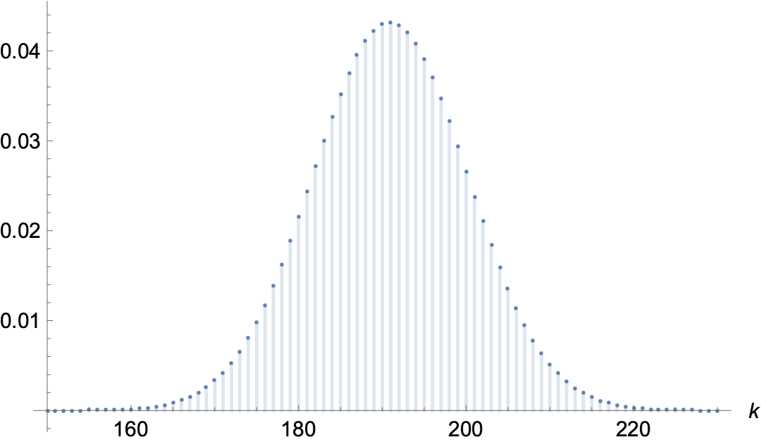
(a)

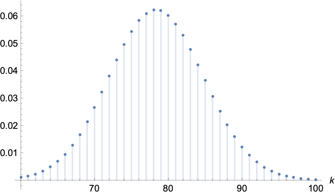
(b)

Figure 3: The ratio $z^{(k)}_{2}/z_{2}^{(0)}$ in (85). (a) $N=1000,q=2$, the $y$ axis labels $\frac{s_{k}}{\sum_{i=0}^{p}s_{i}}$. The peak is of order $1/\sqrt{N}$. (b) $N=1000,q=4$, the $y$ axis labels $\frac{s_{k}}{\sum_{i=0}^{p}s_{i}}$. The peak is of order $1/\sqrt{N}$.

As we found in Peng:2022pfa $\langle z^{2}\rangle$ can be computed by a trick of introducing the collective variables

$$G_{LR}=\frac{1}{N}\sum_{i}\psi_{i}^{L}\psi_{i}^{R},\quad G_{L}=\frac{1}{N}\sum_{i<j}\psi_{i}^{L}\psi_{j}^{L},\quad G_{R}=\frac{1}{N}\sum_{i<j}\psi_{i}^{R}\psi_{j}^{R}\,,$$ (86)

and doing the path integral. The final expression is

$$\langle z^{2}\rangle = \int_{R}\operatorname{d}^{3}G_{i}\int_{\text{i}\mathbb{R}}\operatorname{d}^{3}\Sigma_{i}\,e^{\frac{N}{q}(\tau^{2}G_{LR}^{q}+\mu G_{L}^{q/2}+\mu G_{R}^{q/2})-N(\Sigma_{i}G_{i})}\frac{1}{2}\left((\Sigma_{LR}+\text{i}\sqrt{\Sigma_{L}\Sigma_{R}})^{N}+(\Sigma_{LR}-\text{i}\sqrt{\Sigma_{L}\Sigma_{R}})^{N}\right)$$

$$= \int_{R}\operatorname{d}^{3}G_{i}\int_{\text{i}\mathbb{R}}\operatorname{d}^{3}\Sigma_{i}\,\sum_{m=0}^{N/2}{N\choose 2m}(\Sigma_{LR})^{2m}(\text{i}^{2}\Sigma_{L}\Sigma_{R})^{\frac{N}{2}-m}e^{\frac{N}{q}(\tau^{2}G_{LR}^{q}+\mu G_{L}^{q/2}+\mu G_{R}^{q/2})}e^{-N(\Sigma_{i}G_{i})}\,,$$

In Peng:2022pfa we indeed find a new non-trivial saddle point whose saddle contribution is larger than the saddle contribution of the trivial disk saddle and wormhole saddle. The new non-trivial saddle should correspond to $\sum_{k}\langle\Theta_{k}^{2}\rangle$ with $k$ in the peak. The expression (2.3) of $\langle z^{2}\rangle$ leads to a $G,\Sigma$ expression of each $z_{2}^{(k)}$

$$\langle\Theta_{k}^{2}\rangle = z_{2}^{(k)}={N\choose kq}\int_{R}\operatorname{d}^{3}G_{i}\int_{\text{i}\mathbb{R}}\operatorname{d}^{3}\Sigma_{i}\,(\Sigma_{LR})^{kq}(\text{i}^{2}\Sigma_{L}\Sigma_{R})^{\frac{N-kq}{2}}e^{\frac{N}{q}(\tau^{2}G_{LR}^{q}+\mu G_{L}^{q/2}+\mu G_{R}^{q/2})}e^{-N(\Sigma_{i}G_{i})}.$$

Actually we can derive a different $G,\Sigma$ expression from $\Theta_{i}$ directly in a more enlightening way. Because $\psi_{i}$ are Grassmann numbers and $q$ is even then the exponential in (57) factorizes

$$e^{\text{i}^{q/2}\sum_{A}J_{A}\psi_{A}}=\prod_{A}e^{\text{i}^{q/2}J_{A}\psi_{A}}.$$ (88)

Using Tyler expansion the definition of $\theta^{(i)}$ one can derive a useful identity

$$e^{\alpha X}=\langle e^{\alpha X}\rangle\sum_{i=0}^{\infty}\frac{\alpha^{n}}{n!}\theta^{(n)},$$ (89)

where $X$ is the random variable. With the help of this identity and $\psi_{A}^{2}=0$, (88) can be decomposed into

$$\prod_{A}e^{\text{i}^{q/2}J_{A}\psi_{A}} = \langle e^{\text{i}^{q/2}\sum_{A}J_{A}\psi_{A}}\rangle\left(1+\sum_{A}\theta_{A}^{(1)}(\text{i}^{q/2}\psi_{A})+\frac{1}{2!}\sum_{A,B}\theta_{A}^{(1)}(\text{i}^{q/2}\psi_{A})\theta_{B}^{(1)}(\text{i}^{q/2}\psi_{B})+\dots\right)$$ (90)

$$= \langle e^{\text{i}^{q/2}\sum_{A}J_{A}\psi_{A}}\rangle e^{\sum_{A}\theta_{A}^{(1)}\psi_{A}}.$$

Thus the we can express $\langle\Theta_{k}^{2}\rangle$ as

$$\langle\Theta_{k}^{2}\rangle=\int\operatorname{d}^{2N}\psi^{L(R)}\langle e^{\text{i}^{q/2}\sum_{A}J_{A}\psi^{L}_{A}}\rangle\langle e^{\text{i}^{q/2}\sum_{A}J_{A}\psi^{R}_{A}}\rangle\frac{1}{k!^{2}}(\text{i}^{q/2}\sum_{A}\psi_{A}^{L}\theta_{A}^{(1)})^{k}(\text{i}^{q/2}\sum_{A}\psi_{A}^{R}\theta_{A}^{(1)})^{k}$$

$$=\int\operatorname{d}^{2N}\psi^{L(R)}\langle e^{\text{i}^{q/2}\sum_{A}J_{A}\psi^{L}_{A}}\rangle\langle e^{\text{i}^{q/2}\sum_{A}J_{A}\psi^{R}_{A}}\rangle\frac{t^{2k}}{k!}(\sum_{A}\psi_{A}^{L}\psi_{A}^{R})^{k}$$ (91)

$$=\int\operatorname{d}^{2N}\psi^{L(R)}\operatorname{d}G_{LR}\operatorname{d}\Sigma_{LR}\,e^{\text{i}^{q/2}u\sum_{A}(\psi_{A}^{L}+\psi_{A}^{R})}e^{-N\Sigma_{LR}(G_{LN}-\sum_{i}\psi_{i}^{L}\psi_{i}^{R})}\frac{1}{k!}\left(\frac{N\tau^{2}}{q}G_{LR}^{q}\right)^{k}$$

$$=\int_{R}\operatorname{d}^{3}G_{i}\int_{\text{i}\mathbb{R}}\operatorname{d}^{3}\Sigma_{i}\,\frac{1}{2}\left((\Sigma_{LR}+\text{i}\sqrt{\Sigma_{L}\Sigma_{R}})^{N}+(\Sigma_{LR}-\text{i}\sqrt{\Sigma_{L}\Sigma_{R}})^{N}\right)$$

$$\qquad\qquad\qquad e^{\frac{N}{q}(\mu G_{L}^{q/2}+\mu G_{R}^{q/2})}e^{-N(\Sigma_{i}G_{i})}\frac{1}{k!}\left(\frac{N\tau^{2}}{q}G_{LR}^{q}\right)^{k}.$$ (92)

The integral (92) is not convergent but we can introduce the generating function

$$F(v)=\int_{R}\operatorname{d}^{3}G_{i}\int_{\text{i}\mathbb{R}}\operatorname{d}^{3}\Sigma_{i}\,\frac{1}{2}\left((\Sigma_{LR}+\text{i}\sqrt{\Sigma_{L}\Sigma_{R}})^{N}+(\Sigma_{LR}-\text{i}\sqrt{\Sigma_{L}\Sigma_{R}})^{N}\right)$$

$$\qquad e^{\frac{N}{q}(v\tau^{2}G_{LR}^{q}+\mu G_{L}^{q/2}+\mu G_{R}^{q/2})}e^{-N(\Sigma_{i}G_{i})},$$ (93)

which can be computed with a saddle point approximation and the $\langle\Theta_{k}^{2}\rangle$ is given by

$$\langle\Theta_{k}^{2}\rangle=\frac{1}{k!}\frac{\operatorname{d}^{k}F(v)_{\text{saddle}}}{\operatorname{d}v^{k}}\Big{|}_{v=0}\,.$$ (94)

As a simple test, we know that the exact result of $F(v)$ is just

$$F(v)=\langle z^{2}\rangle_{t^{2}\rightarrow t^{2}v}=\sum_{k}c_{k}m_{p-k}^{2}t^{2k}u^{2p-2k}v^{k},$$ (95)

which indeed leads to

$$\langle\Theta_{k}^{2}\rangle=\frac{1}{k!}\frac{\operatorname{d}^{k}F(v)_{\text{saddle}}}{\operatorname{d}v^{k}}\Big{|}_{v=0}=c_{k}m_{p-k}^{2}t^{2k}u^{2p-2k}\,.$$ (96)

2.3.1 Half-wormhole in $z^{2}$

To make the half-wormhole saddle manifest below we will set $u=0$. In this case “Bose-Einstein” condensation happens. As found in Saad:2021rcu for the square of partition function $z^{2}$ the wormhole persists and there is only one dominant non-self-averaged sector. Applying (30) directly leads to the decomposition

$$z^{2}=\sum_{i}\Phi_{2i},$$ (97)

with

$$\Phi_{0}=\langle z^{2}\rangle=\sum^{\prime}_{A_{1}(B_{1})<\dots<A_{p}(B_{p})}\text{sgn}(A)\text{sgn}(B)t^{2}\delta_{A_{1}B_{1}}\dots\dots t^{2}\delta_{A_{p}B_{p}},$$ (98)

$$\Phi_{2}=\sum_{k}\sum^{\prime}_{A_{1}(B_{1})<\dots<A_{p}(B_{p})}\text{sgn}(A)\text{sgn}(B)t^{2}\delta_{A_{1}B_{1}}\dots(\theta_{A_{k}}^{(1)}\theta_{B_{k}}^{(1)}+\delta_{A_{k}B_{k}}(\theta_{A_{k}}^{(2)}-{\theta_{A_{k}}^{(1)}}^{2}))\dots t^{2}\delta_{A_{p}B_{p}},$$

$$\dots$$ (99)

$$\Phi_{2p}=\sum^{\prime}_{A_{1}(B_{1})<\dots<A_{p}(B_{p})}\text{sgn}(A)\text{sgn}(B)(\theta_{A_{1}}^{(1)}\theta_{B_{1}}^{(1)}+\delta_{A_{1}B_{1}}(\theta_{A_{1}}^{(2)}-{\theta_{A_{1}}^{(1)}}^{2}))\dots(\theta_{A_{p}}^{(1)}\theta_{B_{p}}^{(1)}+\delta_{A_{p}B_{p}}(\theta_{A_{p}}^{(2)}-{\theta_{A_{p}}^{(1)}}^{2}))$$

where $\Phi_{2p}$ is the half-wormhole saddle which is found in Saad:2021rcu ; Mukhametzhanov:2021hdi by noticing $\theta_{A}^{(1)}=J_{A}$ and $\theta_{A}^{(2)}-{\theta_{A}^{(1)}}^{2}=-t^{2}$. Actually the connection between the half-wormhole proposed in Saad:2021rcu and factorization proposal introduced in Saad:2021uzi has been pointed out in Peng:2021vhs . A useful way to derive the expression of $\Phi_{i}$ is to use (89) first

$$e^{\text{i}^{q/2}\sum_{A}J_{A}(\psi_{A}^{L}+\psi_{A}^{R})}=\prod_{A}e^{\text{i}^{q/2}J_{A}(\psi_{A}^{L}+\psi_{A}^{R})}$$ (101)

$$\quad=\langle e^{\text{i}^{q/2}\sum_{A}J_{A}(\psi_{A}^{L}+\psi_{A}^{R})}\rangle\prod_{A}(1+\text{i}^{q/2}\theta_{A}^{(1)}(\psi_{A}^{L}+\psi_{A}^{R})+\text{i}^{q}\theta_{A}^{(2)}\psi_{A}^{L}\psi_{A}^{R})$$ (102)

$$\quad=\langle e^{\text{i}^{q/2}\sum_{A}J_{A}(\psi_{A}^{L}+\psi_{A}^{R})}\rangle e^{\text{i}^{q/2}\sum_{A}\theta_{A}^{(1)}(\psi_{A}^{L}+\psi_{A}^{R})+\text{i}^{q}\sum_{A}(\theta_{A}^{(2)}-{\theta_{A}^{(1)}}^{2})\psi_{A}^{L}\psi_{A}^{R}}$$ (103)

and then to substitute it into the integral form of $z^{2}$

$$z^{2} = \int\operatorname{d}^{2N}\psi^{L(R)}\langle e^{\text{i}^{q/2}\sum_{A}J_{A}(\psi_{A}^{L}+\psi_{A}^{R})}\rangle e^{\text{i}^{q/2}\sum_{A}\theta_{A}^{(1)}(\psi_{A}^{L}+\psi_{A}^{R})+\text{i}^{q}\sum_{A}(\theta_{A}^{(2)}-{\theta_{A}^{(1)}}^{2})\psi_{A}^{L}\psi_{A}^{R}}$$ (104)

$$= \int\operatorname{d}^{2N}\psi^{L(R)}e^{\text{i}^{q/2}\sum_{A}\theta_{A}^{(1)}(\psi_{A}^{L}+\psi_{A}^{R})+\text{i}^{q}\sum_{A}[(\theta_{A}^{(2)}-{\theta_{A}^{(1)}}^{2})+t^{2}]\psi_{A}^{L}\psi_{A}^{R}}$$

$$= \text{i}^{N}\sum_{k=0}^{p}\int\operatorname{d}^{2N}\psi^{L(R)}\frac{\left(\sum_{A}[(\theta_{A}^{(2)}-{\theta_{A}^{(1)}}^{2})+t^{2}]\psi_{A}^{L}\psi_{A}^{R}\right)^{k}}{k!}\frac{(\sum_{A}\theta_{A}^{(1)}\psi_{A}^{L})^{p-k}}{(p-k)!}\frac{(\sum_{A}\theta_{A}^{(1)}\psi_{A}^{R})^{p-k}}{(p-k)!}$$

$$= \sum^{\prime}_{A(B)}\text{sgn}(A)\text{sgn}(B^{\prime})\prod_{i}(\theta_{A_{i}}^{(1)}\theta_{B_{i}}^{(1)}+\delta_{A_{i}B_{i}}(\theta_{A_{i}}^{(2)}-{\theta_{A_{i}}^{(1)}}^{2}+t^{2})).$$ (106)

By matching the power of $t^{2}$ we can extract the expression of $\Phi_{i}$. Note that the expressions of $\Phi_{i}$ have been derived in Mukhametzhanov:2021hdi based on the proposal of Saad:2021rcu . In Mukhametzhanov:2021hdi the non-dominant sectors are derived as fluctuations of the dominant saddle $\Phi_{2p}$ with the help of introducing $G,\Sigma$ variables. Because our derivation here does not rely on $G,\Sigma$ trick so it can be used to derive possible $n$-linked half-wormholes in $z^{n}$. First we notice that $\langle z^{2}\rangle^{2}=\langle\Phi_{0}^{2}\rangle$ is in the same order of $\langle z^{4}\rangle\approx\langle z^{2}\rangle^{2}$ as proved in Saad:2021rcu so the wormhole saddle persists. To confirm that $\Phi_{2p}$ is the only dominant non-self-averaged saddle we only need to show

$$\langle z^{4}\rangle\approx\langle\Phi_{0}^{2}\rangle+\langle\Phi_{2p}^{2}\rangle,$$ (107)

which also has been proved in Saad:2021rcu ; Mukhametzhanov:2021hdi . Another benefit of the rewriting (104) is that we can introduce $G,\Sigma$ variable directly if needed because the appearance of $\langle e^{\text{i}^{q/2}\sum_{A}J_{A}(\psi_{A}^{L}+\psi_{A}^{R})}\rangle$ instead of introducing them “by hand” by inserting an identity as proposed in Saad:2021rcu . As we argued in Peng:2022pfa when $u\neq 0$, $\Phi_{2p}$ will not be the dominant sector anymore. Instead there will be a package of surviving non-self-averaged sectors.

2.3.2 Half-wormhole in $z^{3}$

As we argued in the statistical toy model, there should exist $n$-linked half-wormholes. For simplicity let us focus on 3-linked half-wormholes and $z^{3}$. Similar to (104), $z^{3}$ can be rewritten as

$$z^{3} = \int\operatorname{d}^{3N}\psi^{i}e^{\text{i}^{q/2}\sum_{A}J_{A}(\psi_{A}^{1}+\psi_{A}^{2}+\psi_{A}^{3})}$$ (109)

$$= \int\operatorname{d}^{3N}\psi^{i}\langle e^{\text{i}^{q/2}\sum_{A}J_{A}(\psi_{A}^{1}+\psi_{A}^{2}+\psi_{A}^{3})}\rangle e^{\text{i}^{q/2}\sum_{A}\theta_{A}^{(1)}(\psi_{A}^{1}+\psi_{A}^{2}+\psi_{A}^{3})}\times$$

$$e^{\text{i}^{q}\sum_{A}(\theta_{A}^{(2)}-{\theta_{A}^{(1)}}^{2})(\psi_{A}^{1}\psi_{A}^{2}+\psi_{A}^{1}\psi_{A}^{3}+\psi_{A}^{2}\psi_{A}^{3})}e^{\text{i}^{3q/2}\sum_{A}(\theta_{A}^{(3)}-3\theta_{A}^{(2)}{\theta_{A}^{(1)}}+2{\theta_{A}^{(1)}}^{3})\psi_{A}^{1}\psi_{A}^{2}\psi_{A}^{3}},$$

$$= \sum_{i=0}^{3p}\Lambda_{i}.$$ (110)

Again the expression of $\Lambda_{i}$ can be extracted by matching the power of $t^{2}$. Since $\langle z^{3}\rangle=0$, so the self-averaged sector does not exist and $z^{3}$ is only dominated by non-self-averaged sectors which we expect are $\Lambda_{3p}$:

$$\Lambda_{3p} = \int\operatorname{d}^{3N}\psi^{i}e^{\text{i}^{q/2}\sum_{A}\theta_{A}^{(1)}(\psi_{A}^{1}+\psi_{A}^{2}+\psi_{A}^{3})}\times$$ (111)

$$e^{\text{i}^{q}\sum_{A}(\theta_{A}^{(2)}-{\theta_{A}^{(1)}}^{2})(\psi_{A}^{1}\psi_{A}^{2}+\psi_{A}^{1}\psi_{A}^{3}+\psi_{A}^{2}\psi_{A}^{3})}e^{\text{i}^{3q/2}\sum_{A}(\theta_{A}^{(3)}-3\theta_{A}^{(2)}{\theta_{A}^{(1)}}+2{\theta_{A}^{(1)}}^{3})\psi_{A}^{1}\psi_{A}^{2}\psi_{A}^{3}},$$

$$= \int\operatorname{d}^{3N}\psi^{i}e^{\text{i}^{q/2}\sum_{A}J_{A}(\psi_{A}^{1}+\psi_{A}^{2}+\psi_{A}^{3})}e^{-\text{i}^{q}t^{2}\sum_{A}(\psi_{A}^{1}\psi_{A}^{2}+\psi_{A}^{1}\psi_{A}^{3}+\psi_{A}^{2}\psi_{A}^{3})},$$ (112)

and $\Lambda_{p}$:

$$\Lambda_{p} = \int\operatorname{d}^{3N}\psi^{1,2,3}\sum_{(i,j,k)=(1,2,3),(1,3,2),(2,3,1)}\left(e^{\text{i}^{q}t^{2}\sum_{A}\psi_{A}^{i}\psi_{A}^{j}}e^{\text{i}^{q/2}\sum_{A}\theta_{A}^{(k)}\psi_{A}^{k}}\right)$$ (113)

$$= 3\langle z^{2}\rangle z,$$ (114)

where we have substituted the explicit expressions of $\theta^{(i)}_{A}$. The term of triple product $\psi_{A}^{1}\psi_{A}^{2}\psi_{A}^{3}$ drops out in $\Lambda_{3p}$ because of $J_{A}$ is Gaussian so that there is no tri-linear interactions. From (112) and (113) it is obvious to show $\langle\Lambda_{3p}\rangle=\langle\Lambda_{p}\rangle=0$ as they should be. To confirm that they are dominant let us compute $\langle\Lambda_{3p}^{2}\rangle$ and $\langle\Lambda_{p}^{2}\rangle$

$$\langle\Lambda_{3p}^{2}\rangle = \langle\Lambda_{3p}^{L}\Lambda_{3p}^{R}\rangle$$ (115)

$$= \int\operatorname{d}^{6N}\psi^{L_{i}(R_{i})}e^{\text{i}^{q}t^{2}\sum_{A}\left(\sum_{i,j=1}^{3}\psi_{A}^{L_{i}}\psi_{A}^{R_{j}}\right)}\approx 6\langle z^{2}\rangle^{3},$$ (116)

$$\langle\Lambda_{p}^{2}\rangle = \langle\Lambda_{p}^{L}\Lambda_{p}^{R}\rangle=9\langle z^{2}\rangle^{3},$$ (117)

which give

$$\langle\Lambda_{3p}^{2}\rangle+\langle\Lambda_{p}^{2}\rangle\approx 15\langle z^{2}\rangle^{3}\approx\langle z^{6}\rangle.$$ (118)

Therefore the approximation

$$z^{3}\approx\Lambda_{p}+\Lambda_{3p},$$ (119)

is the analogue of (38). We believe that this analogy persists for all other higher moments $z^{n}$. Recall that $\theta^{(i)}$ can be thought of as moments thus it is reasonable to introduce the connected moments or the cumulants $\tilde{\theta}^{(i)}$ with those $z^{3}$ can be cast into

$$z^{3}=\int\operatorname{d}^{3N}\psi^{i}\langle e^{\text{i}^{q/2}\sum_{A}J_{A}(\psi_{A}^{1}+\psi_{A}^{2}+\psi_{A}^{3})}\rangle\prod_{k}e^{\text{i}^{kq/2}\sum_{A}\tilde{\theta}_{A}^{(k)}\frac{(\sum_{i}\psi_{A}^{i})^{k}}{k!}}.$$ (120)

In general, we expect

$$z^{n}=\int\operatorname{d}^{nN}\psi^{i}\langle e^{\text{i}^{q/2}\sum_{A}J_{A}(\sum_{i=1}^{n}\psi_{A}^{i})}\rangle\prod_{k=1}^{n}e^{\text{i}^{kq/2}\sum_{A}\tilde{\theta}_{A}^{(k)}\frac{(\sum_{i}\psi_{A}^{i})^{k}}{k!}},$$ (121)

which is simple to check for small $n$ by a direct calculation. Since $\theta^{(i)}$ is Gaussian so the only non-vanishing cumulants are $\tilde{\theta}^{(1)}$ and $\tilde{\theta}^{(2)}$ thus

$$z^{n}=\int\operatorname{d}^{nN}\psi^{i}\langle e^{\text{i}^{q/2}\sum_{A}J_{A}(\sum_{i=1}^{n}\psi_{A}^{i})}\rangle e^{\text{i}^{q/2}\sum_{A}\theta_{A}^{(1)}(\sum_{i}\psi_{A}^{i})}e^{\text{i}^{q}\frac{1}{2}\sum_{A}\tilde{\theta}_{A}^{(2)}(\sum_{i}\psi_{A}^{i})^{2}}.$$ (122)

As a consistency check, substituting the explicit expressions $\theta^{(1)}_{A}=J_{A}$ and $\tilde{\theta}^{(2)}_{A}=-t^{2}$ into (122) leads to $z^{n}$ directly as it should be since (122) is nothing but a rewriting of $z^{n}$ in a convenient way of extracting contributions from different sectors and it is a direct generalization of the trick introduced in Saad:2021rcu . In particular the highest level sector of $z^{n}$ can be expressed as

$$\Theta=\int\operatorname{d}^{nN}\psi^{i}e^{\text{i}^{q/2}\sum_{A}\theta_{A}^{(1)}(\sum_{i}\psi_{A}^{i})}e^{\text{i}^{q}\frac{1}{2}\sum_{A}\tilde{\theta}_{A}^{(2)}(\sum_{i}\psi_{A}^{i})^{2}},$$ (123)

which is expected to be one of the dominant non-self-averaged sector in the large $N$ limit.

2.4 0+1 SYK model

Now let us apply our proposal to the 1-SYK model. The partition function is defined as

$$z(\beta)=\int D\psi\,\exp\left\{-\int_{0}^{\beta}\operatorname{d}\tau\left(\psi_{i}\partial_{\tau}\psi_{i}+\text{i}^{q/2}J_{A}\psi_{A}\right)\right\},$$ (124)

with $J_{A}$’s satisfy (51). We will assume that (122) is approximately valid at least semi-classically. In other words, the saddle point can be derived from (122). The possible problem of (122) in one-dimensional SYK model is that the fermions are not Grassmann numbers but Majorana fermions. As a result, $\psi_{A}$ does not commute with $\psi_{B}$ if there are odd number common indexes in the collective indexes $A$ and $B$. Therefore (89) is not exact anymore. The reason why we expect such subtlety is negligible in the large $N$ limit is because when we introduce standard $G,\Sigma$ variables in the SYK model we already ignore this fact and it is shown in Saad:2018bqo this approximation is correct in the large $N$ limit.

2.4.1 Half-wormhole in $z$ and complex coupling

First let us consider $z(\beta+\text{i}T)$

$$z(\beta+\text{i}T)=\int D\psi\,e^{-\int_{0}^{\beta}\operatorname{d}\tau\left(\psi_{i}\partial_{\tau}\psi_{i}\right)+t^{2}\sum_{A}\mathcal{O}_{A}\mathcal{O}_{A}}e^{\sum_{A}\theta_{A}^{(1)}\mathcal{O}_{A}}e^{\sum_{A}\tilde{\theta}_{A}^{(2)}\mathcal{O}_{A}\mathcal{O}_{A}},$$ (125)

where we have defined the operator

$$\mathcal{O}_{A}(\beta+\text{i}T)\equiv\text{i}^{q/2}\int_{0}^{\beta+\text{i}T}\operatorname{d}\tau_{A}\psi_{A}.$$ (126)

The reason we consider $z(\beta+\text{i}T)$ is that its square $\langle z(\beta+\text{i}T)z(\beta-\text{i}T)\rangle$ is the spectral form factor (SFF) which has universal behaviors for chaotic systems like SYK model and random matrix theories. When $T$ is small, SFF is self-averaged so it is dominated by disconnected piece $\langle z(\beta+\text{i}T)z(\beta-\text{i}T)\rangle\approx\langle z(\beta+\text{i}T\rangle\langle z(\beta-\text{i}T)\rangle$. Because the one point function decays with respect to time and so is SFF. This decay region of SFF is called the slope. Because of the chaotic behavior SSF should not vanish in the late time. It will be the non-self-averaged sector dominates which are responsible for the ramp of the SFF. Therefore, in the ramp region we expect the approximation

$$z\approx\Theta(\beta+\text{i}T) \equiv \int D\psi\,e^{-\int_{0}^{\beta+\text{i}T}\operatorname{d}\tau\psi_{i}\partial_{\tau}\psi_{i}}e^{\sum_{A}\theta_{A}^{(1)}\mathcal{O}_{A}}e^{\sum_{A}\tilde{\theta}_{A}^{(2)}\mathcal{O}_{A}\mathcal{O}_{A}}$$ (127)

$$= \int D\psi\,e^{-\int_{0}^{\beta+\text{i}T}\operatorname{d}\tau\psi_{i}\partial_{\tau}\psi_{i}}e^{\sum_{A}\theta_{A}^{(1)}\mathcal{O}_{A}}e^{-\frac{t^{2}}{2}\sum_{A}\mathcal{O}_{A}\mathcal{O}_{A}},$$ (128)

which is the analog of the highest level sector (123) in the 0d SYK model. It can also be written as $\langle e^{\sum_{A}\theta_{A}^{(1)}\mathcal{O}_{A}}\rangle_{\overline{SYK}}$, where $\overline{SYK}$ can be thought of as the anti-SYK model which is a SYK model but with an opposite bi-linear coupling or it can be think of as a SYK model with purely imaginary random coupling $\text{i}\tilde{J}_{A}$. The relation between factorization and complex couplings in SYK model was also proposed in Mukhametzhanov:2021hdi . To confirm this approximation, let us compute

$$\langle\Theta(\beta+\text{i}T)\Theta(\beta-\text{i}T)\rangle = \int D\psi^{L}D\psi^{R}e^{-\int_{0}^{\beta\pm\text{i}T}\operatorname{d}\tau\psi_{i}^{L(R)}\partial_{\tau}\psi_{i}^{L(R)}}e^{-\frac{t^{2}}{2}(\mathcal{O}_{A}^{L}\mathcal{O}_{A}^{L}+\mathcal{O}_{A}^{R}\mathcal{O}_{A}^{R})}\times$$ (129)

$$\langle e^{\sum_{A}\theta_{A}^{(1)}\mathcal{O}_{A}^{L}}e^{\sum_{A}\theta_{A}^{(1)}\mathcal{O}_{A}^{R}}\rangle$$

$$= \int D\psi^{L}D\psi^{R}e^{-\int_{0}^{\beta\pm\text{i}T}\operatorname{d}\tau\psi_{i}^{L(R)}\partial_{\tau}\psi_{i}^{L(R)}}e^{t^{2}\sum_{A}\mathcal{O}_{A}^{L}\mathcal{O}_{A}^{R}},$$ (130)

which describes the wormhole saddle considering that we can introduce the $G_{LR}$ as

$$t^{2}\sum_{A}\mathcal{O}^{L}_{A}\mathcal{O}^{R}_{A}\approx\frac{t^{2}}{q!}\int\operatorname{d}\tau_{L}\int\operatorname{d}\tau_{R}(\sum_{i}\psi_{i}^{L}\psi_{i}^{R})^{q}\equiv\frac{N\tau^{2}}{q}\int\operatorname{d}\tau_{L}\int\operatorname{d}\tau_{R}G_{LR}^{q}.$$ (131)

so the saddle point solution of (130) is the same saddle point solution of $\langle z^{2}\rangle$ with $G_{LL}=G_{RR}=0$. Such solutions are found in Saad:2018bqo . To be more precise, these solutions found in Saad:2018bqo are time-dependent and only in the ramp region we have $G_{LL},G_{RR}\rightarrow 0$. This is why we stress that only in the ramp region our approximation is good. Away from this region, we have to include other sectors which can be obtained by the expansion (125) as

$$\Theta_{k} = \int D\psi\,e^{-\int_{0}^{\beta}\operatorname{d}\tau\left(\psi_{i}\partial_{\tau}\psi_{i}\right)}e^{\sum_{A}\theta_{A}^{(1)}\mathcal{O}_{A}}e^{\sum_{A}\tilde{\theta}_{A}^{(2)}\mathcal{O}_{A}\mathcal{O}_{A}}\left(\frac{(t^{2}\sum_{A}\mathcal{O}_{A}\mathcal{O}_{A})^{k}}{k!}\right),$$ (132)

$$\approx \frac{1}{k!}\left\langle e^{\sum_{A}\theta_{A}^{(1)}\mathcal{O}_{A}}\left(\frac{N\tau^{2}}{q}G_{LL}^{q}\right)^{k}\right\rangle_{\overline{SYK}}.$$ (133)

2.4.2 Half-wormhole in $z^{2}$ and factorization

Let us consider $z(\text{i}T)z(-\text{i}T)$ and apply our decomposition proposal (122)

$$z(\text{i}T)z(-\text{i}T)=\int D\psi^{L(R)}\,e^{S_{SYK}^{L}+S_{SYK}^{R}}e^{\sum_{A}\theta_{A}^{(1)}(\mathcal{O}_{A}^{L}+\mathcal{O}_{A}^{R})}e^{\frac{1}{2}\sum_{A}\tilde{\theta}_{A}^{(2)}(\mathcal{O}_{A}^{L}+\mathcal{O}_{A}^{R})^{2}}.$$ (134)

Motivated by the result of 0-SYK model, we expect that there is also a ramp region where the dominant non-self-averaged sector is given by the 2-linked half-wormhole

$$\Phi = \int D\psi^{L(R)}\,e^{\sum_{A}\theta_{A}^{(1)}(\mathcal{O}_{A}^{L}+\mathcal{O}_{A}^{R})}e^{\frac{1}{2}\sum_{A}\tilde{\theta}_{A}^{(2)}(\mathcal{O}_{A}^{L}+\mathcal{O}_{A}^{R})^{2}}$$ (135)

$$= \int D\psi^{L(R)}\,e^{\sum_{A}\theta_{A}^{(1)}(\mathcal{O}_{A}^{L}+\mathcal{O}_{A}^{R})}e^{-\frac{t^{2}}{2}\sum_{A}(\mathcal{O}_{A}^{L}+\mathcal{O}_{A}^{R})^{2}}$$ (136)

$$= \int D\psi^{L(R)}\,e^{\sum_{A}\theta_{A}^{(1)}(\mathcal{O}_{A}^{L}+\mathcal{O}_{A}^{R})}e^{-\frac{t^{2}}{2}\sum_{A}\left(\mathcal{O}_{A}^{L}\mathcal{O}_{A}^{L}+\mathcal{O}_{A}^{R}\mathcal{O}_{A}^{R}+\mathcal{O}_{A}^{L}\mathcal{O}_{A}^{R}+\mathcal{O}_{A}^{R}\mathcal{O}_{A}^{L}\right)}.$$ (137)

Our proposal (137) of the 2-linked half-wormhole is very close to the one proposed in Mukhametzhanov:2021hdi which has two more bi-linear terms $\mathcal{O}_{A}^{L}\mathcal{O}_{A}^{L}+\mathcal{O}_{A}^{R}\mathcal{O}_{A}^{R}$ in the second exponent. It seems that our proposal is more proper considering that in $\langle\Phi^{2}\rangle$ there are only bi-linear correlations between $L(R)$ and $L^{\prime}(R^{\prime})$

$$\langle\Phi^{2}\rangle= \int D\psi^{L}D\psi^{R}e^{-\int\operatorname{d}\tau\psi_{i}^{L(R)}\partial_{\tau}\psi_{i}^{L(R)}}\int D\psi^{L^{\prime}}D\psi^{R^{\prime}}e^{-\int\operatorname{d}\tau\psi_{i}^{L^{\prime}(R^{\prime})}\partial_{\tau}\psi_{i}^{L^{\prime}(R^{\prime})}}$$ (138)

$$e^{t^{2}\sum_{A}(\mathcal{O}_{A}^{L}\mathcal{O}_{A}^{L^{\prime}}+\mathcal{O}_{A}^{L}\mathcal{O}_{A}^{R^{\prime}}+\mathcal{O}_{A}^{R}\mathcal{O}_{A}^{L^{\prime}}+\mathcal{O}_{A}^{R}\mathcal{O}_{A}^{R^{\prime}})},$$

as shown in Fig. 4. Thus it implies the approximate factorization

$$\text{Error}=z^{2}-\langle z^{2}\rangle-\Phi,$$ (139)

$$\langle\text{Error}^{2}\rangle\approx\langle z^{4}\rangle-\langle z^{2}\rangle^{2}-2\langle\Phi z^{2}\rangle+\langle\Phi^{2}\rangle\approx(3-1-4+2)\langle z^{2}\rangle^{2}\approx 0,$$ (140)

where we have assumed in the regime where the wormhole dominates the partition function $z$ approximates a Gaussian random variable. The bulk point of view of the factorization is also interesting. The insertion of $e^{\sum_{A}\theta_{A}^{(1)}(\sum_{i=1}^{n}\mathcal{O}^{i}_{A})}$ can be thought of inserting spacetime branes in the gravity path integral and the opposite bi-linear coupling means the wormhole amplitudes connecting the branes are opposite to the usual spacetime wormhole amplitudes such that including all the effects of wormholes and branes factorization is achieved. In Blommaert:2021fob , it is proposed that JT gravity can be factorized by inserting such spacetime branes.

Figure 4: The illustration of (138).

2.5 Random Matrix Theory

In this section, let us apply our proposal to the Random Matrix Theory: the GUE ensemble which can also be thought of the CGS model with End-Of-World (EOW) branes. The random matrix element $H_{ij}$ is identified with a EOW brane $(\hat{\psi}_{i},\hat{\psi}_{j})$ in the notation of Marolf:2020xie or the topological complex matter field $Z_{\psi^{\dagger}\psi}$ in the notation of Peng:2021vhs with the restriction that the disk amplitude of $(\hat{\psi}_{i},\hat{\psi}_{i})$ vanishes i.e. $\langle(\hat{\psi}_{i},\hat{\psi}_{i})\rangle=0$. The equivalence between these two models can be understood as the following. The correlation functions of $H_{ij}$ are computed by the Wick contractions which exactly describe how to connect different EOW branes $(\hat{\psi}_{i},\hat{\psi}_{j})$ with spacetime wormholes in the Disk-Cylinder approximation. Therefore the correlation functions of the random matrix theory are equal to the gravity path integral as we have seen in the CGS model. In this theory, we are interested in the observable

$$z(\beta)={\rm Tr}(e^{-\beta H})\,,$$ (141)

whose ensemble average is given by

$$\langle z\rangle=\int\operatorname{d}{H}\,e^{-\frac{1}{2t^{2}}{\rm Tr}H^{2}}z\,,$$ (142)

where $t^{2}$ is usually taken to be $1/N$.

2.5.1 Half-wormhole

First let us consider the non-self-averaged sector in $z$. It is useful to study a simpler observable ${\rm Tr}H^{n}$ to get some intuitions about the non-self-averaged sector of matrix functions. For the random variable $H_{ij}$ we can not use the decomposition (30) directly. One possible way of adapting to (30) is to rewrite $H_{ij}$ as a linear combination of the Gaussian random variables. However this rewriting is not very convenient. Alternatively, we can transfer the matrix integral into the integral over eigenvalues

$$\mathcal{Z}(H)=\int\operatorname{d}He^{-\frac{1}{2t^{2}}{\rm tr}{H^{2}}}=\int\prod_{i}\operatorname{d}\lambda_{i}e^{-\frac{1}{2t^{2}}\sum_{i}\lambda_{i}^{2}}\Delta(\lambda)^{2},$$ (143)

where $\Delta(\lambda)$ is the Vandermonde determinant

$$\Delta(\lambda)=\prod_{i<j}^{L}(\lambda_{i}-\lambda_{j}).$$ (144)

Then the simple single-trace observable translates to

$${\rm Tr}H^{n}=\sum_{i}\lambda_{i}^{n}\,.$$ (145)

However those eigenvalues are not Gaussian random variables. As a result, even though we can still do the sector decomposition but the resulting different sectors are not orthogonal anymore. Although when the level is finite, we can obtain a new orthogonal basis by a direct diagonalization but it is still very cumbersome. We will make some preliminary analysis beyond Gaussian distribution in next section. Here we will take a similar approach as before. Considering the non-vanishing correlator $\langle H_{ij}H_{ji}\rangle=t^{2}$ we should define

$$\theta_{ij}^{(1)}=H_{ij},\quad\theta_{ij,ji}^{(2)}=\theta_{ij}^{(1)}\theta_{ji}^{(1)}-t^{2},$$ (146)

thus we have

$$H_{ij}H_{km} = \langle H_{ij}H_{km}\rangle+\theta_{ij}^{(1)}\theta_{km}^{(1)}+\delta_{jk}\delta_{im}(\theta^{(2)}_{ij,ji}-\theta_{ij}^{(1)}\theta_{ji}^{(1)})$$ (147)

$$\equiv \langle H_{ij}H_{km}\rangle+[H_{ij}H_{km}]$$ (148)

and

$$H_{ij}H_{kl}H_{mn}=\sum_{i=0}^{3}\Theta_{i},\quad\Theta_{0}=\langle H_{ij}H_{kl}H_{mn}\rangle,\quad\Theta_{2}=0,$$ (149)

$$\Theta_{1}=\theta_{ij}^{(1)}\langle H_{kl}H_{mn}\rangle+\theta_{kl}^{(1)}\langle H_{ij}H_{mn}\rangle+\theta_{mn}^{(1)}\langle H_{kl}H_{ij}\rangle,$$ (150)

$$\Theta_{3}=\begin{cases}\theta_{ij}^{(1)}\theta_{kl}^{(1)}\theta^{(1)}_{mn},\quad\text{no pairs like }\eqref{pair}\\ \theta_{ab,ba}^{(2)}\theta_{ji}^{(1)}=\theta_{ab}^{(1)}\theta_{ba}^{(1)}\theta_{ji}^{(1)}-t^{2}\theta_{ji}^{(1)},\quad\text{there is only one pair like }\eqref{pair}\\ \theta_{ab,ba,ab}^{(3)}=\theta_{ab}^{(1)}\theta_{ba}^{(1)}\theta_{ab}^{(1)}-2t^{2}\theta_{ab}^{(1)},\quad a\neq b\\ \theta_{aa,aa,aa}^{(3)}={\theta_{aa}^{(1)}}^{3}-3t^{2}\theta_{aa}^{(1)}.\end{cases},$$ (151)

$$\quad~{}=\theta_{ij}^{(1)}\theta_{kl}^{(1)}\theta^{(1)}_{mn}-\left(\text{all the possible contractions}\right)\equiv[\theta_{ij}^{(1)}\theta_{kl}^{(1)}\theta^{(1)}_{mn}].$$ (152)

So the highest level sector can also be understood as the observable in the “normal order”. Applying this rule of decomposition to the single-trace observables we get

$${\rm Tr}H={\rm Tr}\theta^{(1)},$$ (153)

$${\rm Tr}H^{2}=\langle{\rm Tr}H^{2}\rangle+\sum_{ij}\theta_{ij}^{(2)}=\langle{\rm Tr}H^{2}\rangle+\left({\rm Tr}{\theta^{(1)}}^{2}-N^{2}t^{2}\right),$$ (154)

$${\rm Tr}H^{3}=3\langle{\rm Tr}H^{2}\rangle{\rm Tr}\theta^{(1)}+\left({\rm Tr}({\theta^{(1)}}^{3})-3Nt^{2}{\rm Tr}\theta^{(1)}\right),$$ (155)

$${\rm Tr}H^{4}=\langle{\rm Tr}H^{4}\rangle+\left(4N^{2}t^{2}{\rm Tr}(\theta^{(2)})+2t^{2}[{\rm Tr}\theta^{(1)}{\rm Tr}\theta^{(1)}]\right)+[{\rm Tr}{\theta^{(1)}}^{4}],$$ (156)

$$\dots$$

where the normal ordered terms are explicitly given by

$$[{\rm Tr}\theta^{(1)}{\rm Tr}\theta^{(1)}]={\rm Tr}\theta^{(1)}{\rm Tr}\theta^{(1)}-Nt^{2},$$ (157)

$$[{\rm Tr}{\theta^{(1)}}^{4}]={\rm Tr}{\theta^{(1)}}^{4}-\left(\langle{\rm Tr}H^{4}\rangle+\left(4N^{2}t^{2}{\rm Tr}(\theta^{(2)})+2t^{2}[{\rm Tr}\theta^{(1)}{\rm Tr}\theta^{(1)}]\right)\right).$$ (158)

Like the Wick transformation in quantum field theory, the normal order or the highest level sector can be defined as

$$[f(H)]=e^{-\frac{t^{2}}{2}{\rm Tr}\left(\frac{\delta}{\delta H_{ij}}\frac{\delta}{\delta H_{ji}}\right)}f(H),$$ (159)

or we can introduce the formal integral

$$[f(H)]=\int\operatorname{d}\tilde{H}\,e^{\frac{1}{2t^{2}}{\rm Tr}\tilde{H}^{2}}e^{-\frac{1}{t^{2}}{\rm Tr}(\theta^{(1)}\tilde{H})}e^{\frac{1}{2t^{2}}{\rm Tr}{\theta^{(1)}}^{2}}f(\tilde{H})-f(0),$$ (160)

which is more convenient sometimes. Therefore we can rewrite the decomposition as

$$f(H)=[f(H)]+\sum_{k}Con_{k},$$ (161)

where the $Con_{k}$ means choosing all possible $k$ pairs of matrix elements from $[f(H)]$ and replacing each pair $H_{ab}H_{cd}$ with its expectation value $\langle H_{ab}H_{cd}\rangle$. It implies the identification

$$[f(H)]=\Theta_{p},\quad Con_{k}=\Theta_{p-2k}.$$ (162)

For these single-trace observables, in the large $N$ limit their correlation functions factorize so the dominant sector is always the self-averaged sector. The more interesting observable is $z(\text{i}T)$ whose expectation value is

$$\lim_{N\rightarrow\infty}\langle z(\text{i}T)\rangle = \sum_{k=0}\frac{(\text{i}T)^{2k}}{(2k)!}\langle{\rm Tr}H^{2k}\rangle=N\sum_{k=0}\frac{(\text{i}T\sqrt{Nt^{2}})^{2k}}{(2k)!}C_{k}$$ (163)

$$= N\frac{J_{1}(2\alpha T)}{\alpha T}\sim 0,\quad\text{when }T>>1,$$ (164)

where $C_{k}$ is famous Catalan number and $\alpha=\sqrt{Nt^{2}}$. So in the late time, the non-self-averaged sector becomes important. The lowest sector can be simply obtained by expanding $z$ and picking the term with $\theta^{(1)}$:

$$\Theta_{1} = {\rm Tr}\theta^{(1)}\frac{1}{N}\left(N\text{i}T+\frac{(\text{i}T)^{3}}{3!}3\times\langle{\rm Tr}H^{2}\rangle+\frac{(\text{i}T)^{5}}{5!}5\times\langle{\rm Tr}H^{4}\rangle+\dots\right)$$ (165)

$$= \text{i}{{\rm Tr}\theta^{(1)}}\frac{J_{1}(2\alpha T)}{\alpha}\,.$$ (166)

Similarly we find that the next sector is

$$\Theta_{2} = {\rm Tr}\theta^{(2)}\frac{1}{\alpha^{2}}\left(\frac{(\text{i}T\alpha)^{2}}{2}+\frac{(\text{i}T\alpha)^{4}}{4!}\times 4+\frac{(\text{i}T\alpha)^{6}}{6!}\times(6*2+3)+\dots\right),$$ (167)

$$= -{\rm Tr}\theta^{(2)}\frac{J_{2}(2T\alpha)}{\alpha^{2}},$$ (168)

where we have dropped the terms ${\rm Tr}\theta^{(1)}{\rm Tr}\theta^{(1)}$ because they are suppressed by $1/N$. Comparing with the known results of the wormhole contribution to $\langle z(\text{i}T_{1})z(\text{i}T_{2})\rangle_{c}$

$$\langle z(\text{i}T_{1})z(\text{i}T_{2})\rangle_{c}=\sum_{l=0}^{\infty}(l+1)(-1)^{l+1}J_{l+1}(2\alpha T_{1})J_{l+1}(2\alpha T_{2}),$$ (169)

we will show in the Appendix A that

$$\Theta_{k}=(\text{i})^{k}\frac{J_{k}(2\alpha T)}{\alpha^{k}}{\rm Tr}\theta^{(k)},\quad k>0.$$ (170)

We plot $\langle\Theta_{0}^{2}\rangle+\langle\Theta_{k}^{2}\rangle$ in Fig.6(a) and $\langle\Theta_{k}^{2}\rangle$ in Fig.6(b). The result is very interesting. We see that every curve has the typical slop, ramp and plateau regimes. Another interesting fact is that only the first few sectors contribute to the slop and ramp regions. For example, adding the first 20 sectors we find that the ramp region is roughly located at $[2.5/\alpha,4/\alpha]$ and we plot the contribution of each sector in Fig. 5. Actually including the first 10 sectors is a very good approximation

$$\frac{\sum_{i=1}^{10}\langle\Theta_{i}^{2}\rangle}{\sum_{i=1}^{20}\langle\Theta_{i}^{2}\rangle}=0.999974.$$ (171)

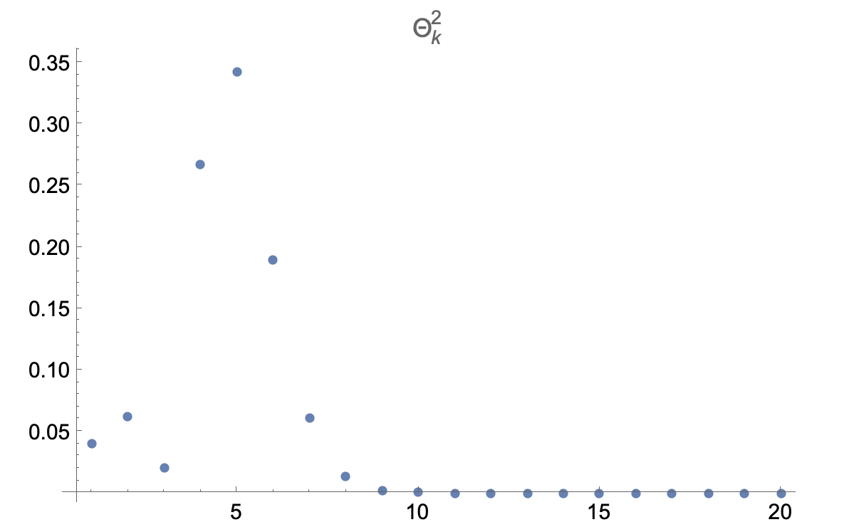
Figure 5: $\alpha=1,T=3.$

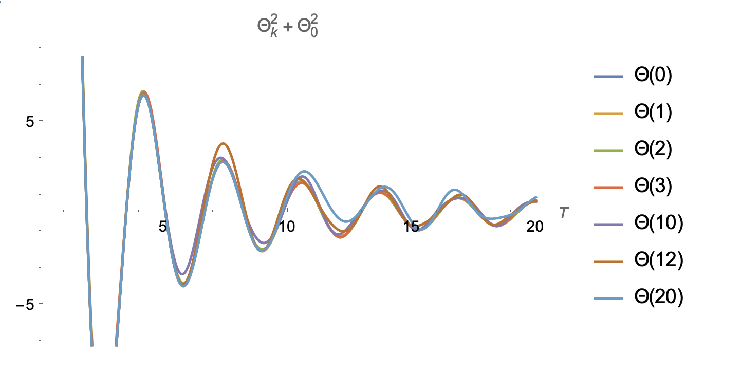
(a) $N=100,\quad\alpha=1$

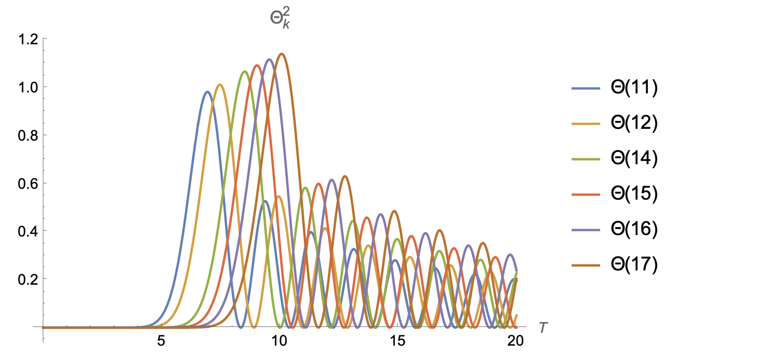
(b) $N=100,\quad\alpha=1$

Figure 6:

Therefore if we only focus on the ramp which is supposed to relate to wormholes we only need to include the first 10 non-self-averaged sectors. In this sense we may call $\Theta=\sum_{i=1}^{10}\Theta_{i}$ the half-wormhole of $z$. This is similar to the half-wormhole of the simple exponential observable (41) in the regime $\beta^{2}t^{2}<1$. We can follow the same procedure to study the decomposition and the half-wormhole of $z^{2}$. But it is very cumbersome and we expect the its behavior is similar to the exponential observable.

3 Beyond Gaussian distribution or the generalized CGS model

One of simplest way to go beyond CGS model is again starting from the MM model but including connected spacetimes with other topologies in the Euclidean path integral. So the next simplest case beyond CGS model is the Disk-Cylinder-Pants model. Let the amplitudes of the disk, cylinder and pants to be

$$\langle\hat{Z}\rangle=\kappa_{1},\quad\langle\hat{Z}^{2}\rangle-\langle\hat{Z}\rangle^{2}=\kappa_{2},\quad\langle\hat{Z}^{3}\rangle-3\langle\hat{Z}\rangle\langle\hat{Z}^{2}\rangle+2\langle\hat{Z}\rangle^{2}=\kappa_{3}.$$ (172)

The generating function is

$$\langle e^{u\hat{Z}}\rangle=\exp\left(u\kappa_{1}+\frac{u^{2}\kappa_{2}}{2!}+\frac{u^{3}\kappa_{3}}{3!}\right),$$ (173)

so we can also identify $\hat{Z}$ as a random variable albeit with a very complicated PDF. We can simply think of the distribution is defined by the same generating function. In Peng:2022pfa we introduce the connected correlators to decompose $\langle Z^{n}e^{\text{i}kZ}\rangle$ for example

$$\langle Ze^{\text{i}kZ}\rangle=\langle Z\rangle\langle e^{\text{i}kZ}\rangle+\langle Ze^{\text{i}kZ}\rangle_{\text{c}}\,,$$ (174)

$$\langle Z^{2}e^{\text{i}kZ}\rangle=\langle Z^{2}\rangle\langle e^{\text{i}kZ}\rangle+2\langle Z\rangle\langle Ze^{\text{i}kZ}\rangle_{c}+\langle Z^{2}e^{\text{i}kZ}\rangle_{\text{c}},$$ (175)

$$\langle Z^{3}e^{\text{i}kZ}\rangle=\langle Z^{3}\rangle\langle e^{\text{i}kZ}\rangle+3\langle Z^{2}\rangle\langle Ze^{\text{i}kZ}\rangle_{c}+3\langle Z\rangle\langle Z^{2}e^{\text{i}kZ}\rangle_{c}+\langle Z^{3}e^{\text{i}kZ}\rangle_{\text{c}}\,,$$ (176)

$$\dots$$

such that using the trick (9) we can decompose $Z_{\alpha}^{n}$ into different sectors which are exactly like (18)-(21). In other words, the number basis or $\{\theta^{(i)}\}$ is still the basis for decomposition. But $\{\theta^{(i)}\}$ should be determined from the recursion relations (18)-(21). For example, in the Disk-Cylinder-Pants model the first few $\theta^{(i)}$ are

$$\theta^{(1)}=Z-\kappa_{1},\quad\theta^{(2)}={\theta^{(1)}}^{2}-\kappa_{2},\quad\theta^{(3)}={\theta^{(1)}}^{3}-3\kappa_{2}\theta^{(1)}-\kappa_{3}.$$ (177)

Because of the inclusion of new wormholes, the pants, the basis is not orthogonal anymore in the sense

$$\langle\theta^{(i)}\theta^{(j)}\rangle\neq\delta_{ij}.$$ (178)

It is easy to find that

$$\langle\theta^{(1)}\theta^{(2)}\rangle=\kappa_{3},\quad\langle\theta^{(2)}\theta^{(3)}\rangle=6\kappa_{2}\kappa_{3}.$$ (179)

Moreover the matrix $M^{(3)}_{ij}=\langle\theta^{(i)}\theta^{(j)}\rangle,i,j=1,2,3$ is

$$M^{(3)}=\left(\begin{array}[]{ccc}\kappa_{2}&\kappa_{3}&0\\ \kappa_{3}&2\kappa_{2}^{2}&6\kappa_{2}\kappa_{3}\\ 0&6\kappa_{2}\kappa_{3}&6\kappa_{2}^{3}+9\kappa_{3}^{2}\\ \end{array}\right).$$ (183)

Naturally $\theta^{(i)}$ can be understood as the $i$-linked half wormhole as shown in Fig.8 and 8

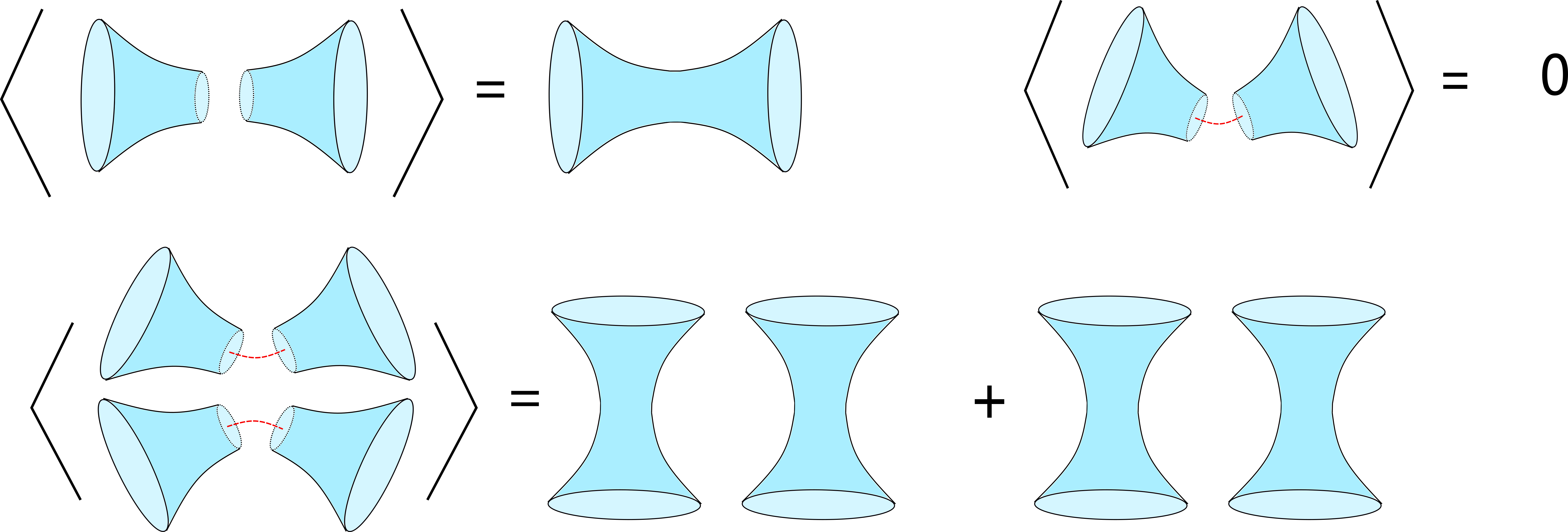
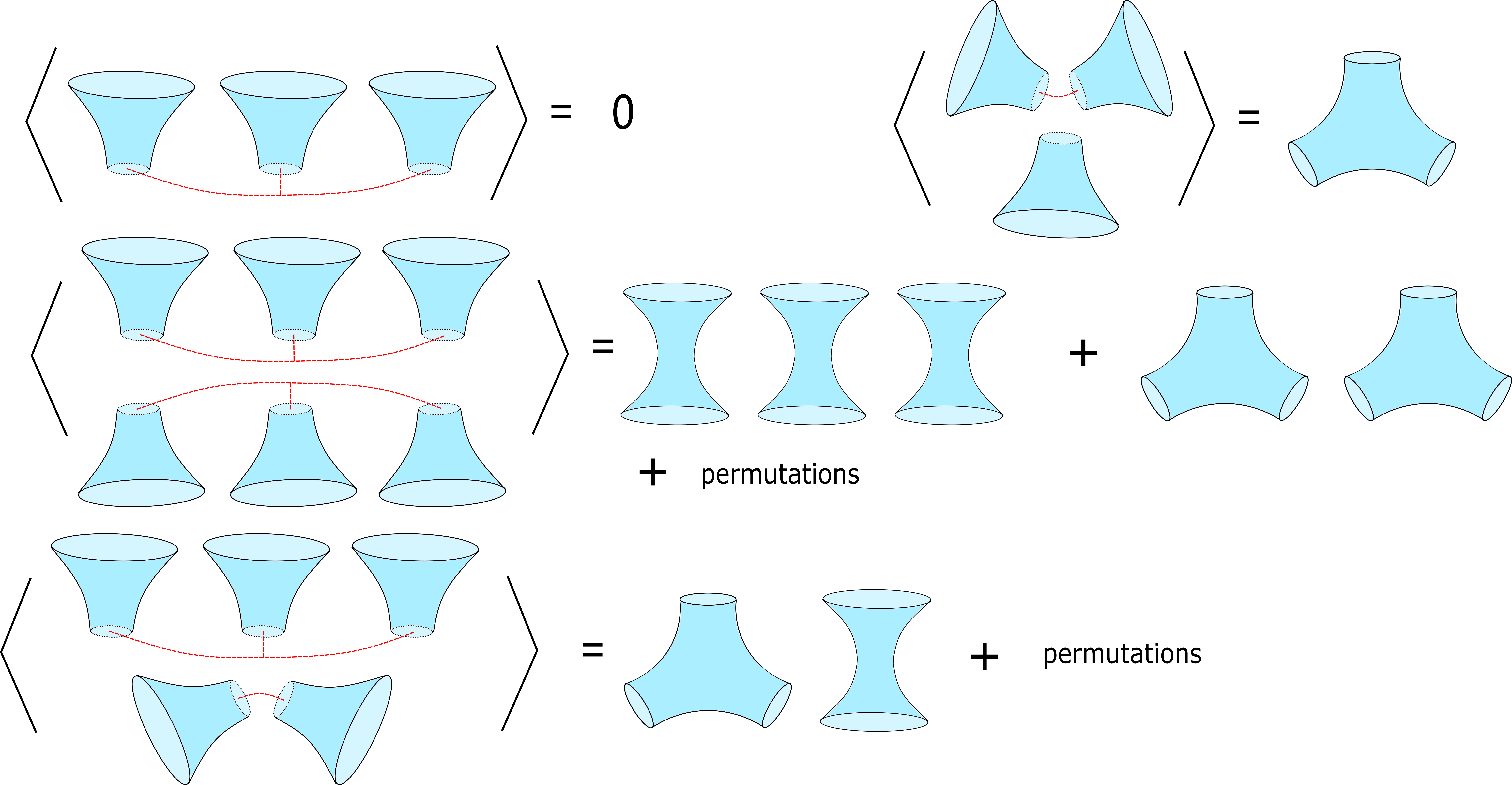
Figure 7: Illustrations of the metric (183)

Figure 8: Illustrations of the metric (183)

3.1 Toy statistical model

We start from the simplest operator

$$Y=\sum_{i}\left(X_{i}-\langle X_{i}\rangle\right).$$ (184)

The modification starts to show up in

$$Y^{3}=\Delta_{0}+\Delta_{1}+\Delta_{3},$$ (185)

where

$$\Delta_{0}=\langle Y^{3}\rangle,$$ (186)

$$\Delta_{1}=3N\kappa_{2}\sum\theta^{(1)}_{i},$$ (187)

$$\Delta_{3}=\sum_{i}\theta^{(3)}_{i}+3\sum_{i\neq j}\theta^{(2)}_{i}\theta^{(1)}_{j}+\sum_{i\neq j\neq k}\theta^{(1)}_{i}\theta^{(1)}_{j}\theta^{(1)}_{k}.$$ (188)

In this special case since $\langle\theta^{(1)}\theta^{(3)}\rangle=0$, there is no cross terms in $\langle Y^{6}\rangle$

$$\langle Y^{6}\rangle=\sum_{i}\langle\Delta_{i}^{2}\rangle,$$ (189)

$$\langle\Delta_{0}^{2}\rangle\sim N^{2}\kappa_{3}^{2},\quad\langle\Delta_{1}^{2}\rangle\sim N^{3}\kappa_{2}^{3},\quad\langle\Delta_{3}^{2}\rangle\sim N^{3}\kappa_{2}^{3}+N^{2}\kappa_{3}^{2},$$ (190)

where we only keep the possible leading terms. When $\kappa_{2},\kappa_{3}\sim\mathcal{O}(1)$, the operator $Y^{3}$ is not self-averaged and the effect of $\kappa_{3}$ is negligible. The interesting case is when $N^{2}\kappa_{3}^{2}>>N^{3}\kappa_{2}^{3}$ so that we have the approximation

$$Y^{3}\approx\langle Y^{3}\rangle+\Delta_{3},$$ (191)

which is the analog of (36).

3.2 0-SYK model

Let us reconsider the 0-SYK model but assume the random couplings satisfying

$$\langle J_{i_{1}\dots i_{q}}\rangle=0,\quad\langle J_{i_{1}\dots i_{q}}J_{j_{1}\dots j_{q}}\rangle=\kappa_{2}\delta_{i_{1}j_{1}}\dots\delta_{i_{q}j_{q}},\quad\kappa_{2}=\tau^{2}\frac{(q-1)!}{N^{q-1}}\ ,$$ (192)

$$\langle J_{A}J_{B}J_{C}\rangle=\kappa_{3}\delta_{ABC},$$ (193)

we will determine the scaling of $\kappa_{3}$ in a moment. Then the averaged quantity is

$$\langle z^{3}\rangle=\int\operatorname{d}^{3N}\psi\,e^{\kappa_{2}\sum_{A}(\psi_{A}^{1}\psi_{A}^{2}+\psi_{A}^{1}\psi_{A}^{3}+\psi_{A}^{2}\psi_{A}^{3})}e^{\text{i}^{3q}\kappa_{3}\sum_{A}\psi_{A}^{1}\psi_{A}^{2}\psi_{A}^{3}},$$ (194)

which can be computed by introducing the collective variables

$$G_{ab} = \frac{1}{N}\sum_{i}\psi_{i}^{a}\psi_{i}^{b},\quad(a,b)=(1,2),(1,3),(2,3),$$ (195)

$$G_{3} = \frac{1}{N}\sum_{i<j}\psi_{i}^{1}\psi_{j}^{1}\psi_{i}^{2}\psi_{j}^{2}\psi_{i}^{3}\psi_{j}^{3},$$ (196)

$$\sum_{A}\psi_{A}^{a}\psi_{A}^{b} = \frac{N^{q}}{q!}G_{ab}^{q},\quad\sum_{A}\psi_{A}^{1}\psi_{A}^{2}\psi_{A}^{3}=\frac{N^{q/2}}{(q/2)!}G_{3}^{q/2},$$ (197)

to rewrite $\langle z^{3}\rangle$ as

$$\langle z^{3}\rangle = \int[\frac{\operatorname{d}G_{ab}\operatorname{d}\Sigma_{ab}}{2\pi\text{i}/N}]\int\frac{\operatorname{d}G_{3}\operatorname{d}\Sigma_{3}}{2\pi\text{i}/N}\,e^{\frac{N}{q}\left(\tau^{2}\sum G_{ab}^{q}+2\gamma^{3}G_{3}^{q/2}\right)}e^{-N(\sum\Sigma_{ab}G_{ab}+\Sigma_{3}G_{3})}$$

$$\quad\int\operatorname{d}^{3N}\psi e^{\Sigma_{ab}\sum_{i}\psi_{i}^{a}\psi_{i}^{b}+\Sigma_{3}\sum_{i<j}\psi_{i}^{1}\psi_{j}^{1}\psi_{i}^{2}\psi_{j}^{2}\psi_{i}^{3}\psi_{j}^{3}}$$

$$= \int[\frac{\operatorname{d}G_{ab}\operatorname{d}\Sigma_{ab}}{2\pi\text{i}/N}]\int\frac{\operatorname{d}G_{3}\operatorname{d}\Sigma_{3}}{2\pi\text{i}/N}\,e^{\frac{N}{q}\left(\tau^{2}\sum G_{ab}^{q}+2\gamma^{3}G_{3}^{q/2}\right)}e^{-N(\sum\Sigma_{ab}G_{ab}+\Sigma_{3}G_{3})}\Sigma_{3}^{N/2}$$

$$= \int\frac{\operatorname{d}G_{3}\operatorname{d}\Sigma_{3}}{2\pi\text{i}/N}\,e^{\frac{N}{q/2}\gamma^{3}G_{3}^{q/2}}e^{-N\Sigma_{3}G_{3}}\Sigma_{3}^{N/2}=\gamma^{3p}m_{p},$$ (199)

where $m_{p}$ is defined in (69) and

$$\gamma^{3}\equiv\text{i}^{3q}\kappa_{3}\frac{N^{q/2-1}}{(q/2-1)!},\quad\gamma\sim\mathcal{O}(1),$$ (200)

thus

$$\kappa_{3}\sim\frac{(q/2-1)!}{N^{q/2}-1}.$$ (201)

Recall that

$$z^{3}=\sum^{\prime}_{A,B,C}\text{sgn}(A)\text{sgn}(B)\text{sgn}(C)J_{A_{1}}J_{B_{1}}J_{C_{1}}\dots J_{A_{p}}J_{B_{p}}J_{C_{p}}.$$ (202)

In general decomposing $z^{3}$ is still very complicated. Let us consider some simple examples. If $p=2$, then we have

$$z^{3} = \sum^{\prime}_{A}\text{sgn}(A)J_{A_{1}}^{3}J_{A_{2}}^{3}+3\sum^{\prime}_{A,B,A_{i}\neq B_{i}}\text{sgn}(B)J_{A_{1}}^{2}J_{A_{2}}^{2}J_{B_{1}}J_{B_{2}}$$ (203)

$$+\sum^{\prime}_{A,B,C,A_{i}\neq B_{i}\neq C_{i}}\text{sgn}(A)\text{sgn}(B)\text{sgn}(C)J_{A_{1}}J_{A_{2}}J_{B_{1}}J_{B_{2}}J_{C_{1}}J_{C_{2}},$$

and there are seven different sectors. A simple way to derive the explicit expression of each sector is to first decompose each $J_{A}^{n}$ as (18)-(21):

$$J_{A}=\theta_{A}^{(1)},\quad J_{A}^{2}=\theta_{A}^{(2)}+(\kappa_{2})_{A},\quad J_{A}^{3}=\theta_{A}^{(3)}+(\kappa_{3})_{A}+3(\kappa_{2})_{A}\theta_{A}^{(1)},$$ (204)

then collect the terms in the same sector:

$$\Delta_{0}=\kappa_{3}^{2}\sum^{\prime}\text{sgn}(A)=m_{p}\kappa_{3}^{2}=\langle z^{3}\rangle,$$ (205)

$$\Delta_{1}=3\kappa_{3}\sum^{\prime}_{A}\text{sgn}(A)\left(\theta_{A_{1}}^{(1)}(\kappa_{2})_{A_{2}}+(\kappa_{2})_{A_{1}}\theta_{A_{2}}^{(1)}\right),$$ (206)

$$\Delta_{2}=(6+3M_{p})\kappa_{2}^{2}\sum^{\prime}_{A}\text{sgn}(A)\theta_{A_{1}}^{(1)}\theta_{A_{2}}^{(1)},$$ (207)

$$\Delta_{3}=\sum^{\prime}_{A}\text{sgn}(A)\left(\theta_{A_{1}}^{(3)}(\kappa_{3})_{A_{2}}+(\kappa_{3})_{A_{1}}\theta_{A_{2}}^{(3)}\right),$$ (208)

$$\Delta_{4}=3\kappa_{2}\sum^{\prime}_{A}\text{sgn}(A)\left(\theta_{A_{1}}^{(3)}\theta_{A_{2}}^{(1)}+\theta_{A_{1}}^{(1)}\theta_{A_{2}}^{(3)}+\sum_{B,B\neq A_{1},A_{2}}\theta_{B}^{(2)}\theta_{A_{1}}^{(1)}\theta_{A_{2}}^{(1)}\right),$$ (209)

$$\Delta_{5}=0,\quad\Delta_{6}=\sum^{\prime}_{A}\text{sgn}(A)\theta_{A_{1}}^{(3)}\theta_{A_{2}}^{(3)}+3\sum^{\prime}_{A,B,A_{i}\neq B_{i}}\text{sgn}(B)\theta_{A_{1}}^{(2)}\theta_{A_{2}}^{(2)}\theta_{B_{1}}^{(1)}\theta_{B_{2}}^{(1)}$$

$$+\sum^{\prime}_{A,B,C,A_{i}\neq B_{i}\neq C_{i}}\text{sgn}(A)\text{sgn}(B)\text{sgn}(C)\theta_{A_{1}}^{(1)}\theta_{A_{2}}^{(1)}\theta_{B_{1}}^{(1)}\theta_{B_{2}}^{(1)}\theta_{C_{1}}^{(1)}\theta_{C_{2}}^{(1)},$$ (210)

where $M_{p}=\frac{(pq)!}{p!(q!)^{p}}$. Now we are ready to compute $\langle\Delta_{i}\Delta_{j}\rangle$ using the relation (183). It turns out that different sectors are still orthogonal for this case:

$$\langle\Delta_{0}^{2}\rangle=m_{p}^{2}\kappa_{3}^{4},\quad\langle\Delta_{1}^{2}\rangle=18M_{p}\kappa_{3}^{2}\kappa_{2}^{3},$$ (211)

$$\langle\Delta_{2}^{2}\rangle=(6+3M_{p})^{2}M_{p}\kappa_{2}^{6},\quad\langle\Delta_{3}^{2}\rangle=2M_{p}\kappa_{3}^{2}(6\kappa_{2}^{3}+9\kappa_{3}^{2}),$$ (212)

$$\langle\Delta_{4}^{2}\rangle=18M_{p}\kappa_{2}^{3}(6\kappa_{2}^{3}+9\kappa_{3}^{2})+18M_{p}(2M_{p}-2)\kappa_{2}^{6},$$ (213)

$$\langle\Delta_{6}^{2}\rangle=M_{p}(6\kappa_{2}^{3}+9\kappa_{3}^{2})^{2}+9M_{p}(M_{p}-1)4\kappa_{2}^{6}+9(m_{p}^{2}-M_{p})\kappa_{3}^{4}$$ (214)

$$\qquad+6M_{p}(M_{p}-1)(M_{p}-2)\kappa_{2}^{6}.$$ (215)

In large $N$ limit the relevant parameters have the following asymptotic behaviors

$$\kappa_{2}\sim\frac{(N/2-1)!}{N^{N/2-1}},\quad\kappa_{3}\sim\frac{(N/4-1)!}{N^{N/4-1}},\quad\kappa_{3}^{2}\sim\kappa_{2}^{3}m_{p}e^{N},\quad M_{p}\sim m_{p}^{2}\sqrt{N},$$ (216)

then the approximation can be given as

$$z^{3}\sim\Delta_{3}+\Delta_{6}.$$ (217)

In general we find that when $p<<N(\text{or }q>>1)$, $z_{3}$ is not self-averaged, i.e. the wormhole does not persists, but the (three-linked) half-wormhole emerges. This fact can be intuitively understood as the following. In this limit because of the scaling (216), the three-mouth-wormhole amplitude is favored thus the possible dominate sectors are $\Delta_{0}$, $\Delta_{3p-3}$ and $\Delta_{3p}$:

$$\langle\Delta_{0}^{2}\rangle=m_{p}^{2}\kappa_{3}^{2p},\quad\langle\Delta_{3p}^{2}\rangle>\langle(\sum^{\prime}_{A}\text{sgn}(A)\theta_{A_{1}}^{(3)}\dots\theta_{A_{p}}^{(3)})^{2}\rangle\sim M_{p}\kappa_{3}^{2p},$$ (218)

$$\langle\Delta_{3p-3}^{2}\rangle>(\sum^{\prime}_{A}\text{sgn}(A)\sum_{i}\theta_{A_{1}}^{(3)}\dots(\kappa_{3})_{A_{i}}\dots\theta_{A_{p}}^{(3)})^{2}\rangle\sim M_{p}\kappa_{3}^{2p},$$ (219)

and since $M_{p}>>m_{p}^{2}$ we conclude that $z^{3}\approx\Delta_{3p-3}+\Delta_{3p}$. This is similar to the result obtained in section 2.3. In the same limit, $z$ is not self-averaged neither while the half-wormhole emerges.

4 Discussion

In this paper we have generalized the factorization proposal introduced in Saad:2021uzi . The main idea is to decompose the observables into the self-averaging sector and non-self-averaging sectors. We find that the contributions from different sectors have interesting statistics in the semi-classical limit. When the self-averaging sector survives in this limit the observable is self-averaging. An interesting phenomenon is the sector condensation meaning the surviving non-self-averaging trend to condense and in the extreme case only one non-self-averaging sector is left-over resembling the Bose-Einstein condensation. Then the half-wormhole saddle is naturally understood as the condensed sectors. We apply the this proposal to simple statistical model , 0-SYK model and random matrix model. Half-wormhole saddles are identified and they are in agreement with the known results. With our proposal we also show the equivalence between the results in Saad:2021uzi and Saad:2021rcu . We also studied multi-linked-half-wormholes and their relations. There are some future directions.

Sector condensation

It is interesting to understand the sector condensation better. We expect that it is some criterion for an ensemble theory or a statistical observable to potentially have a bulk description. So it deserves to study it in other gravity/ensemble theories. Definitely the extreme case mimicking the Bose-Einstein condensation is the most interesting one. We have not understood when it will happen and could it be used as some order parameter. We expect by studying the “phase diagram” in the sector space we can obtain more information about the observables and systems.

Complex coupling and half-wormholes

In Mukhametzhanov:2021hdi , it shows that factorization is related to the complex couplings. In our approach, the complex coupling emerges as an auxiliary parameter to obtain the half-wormhole saddle. The trick here is similar to the one used by Coleman, Giddings and Strominger Coleman:1988cy ; Giddings:1988wv ; Giddings:1988cx , where the non-local effect of spacetime wormhole is “localized” with a price of introducing random couplings. But the current analysis shows that this is only possible when “Bose-Einstein” happens such that the dominant sector can be obtained from this trick. So it would be interesting to explore the relation between complex coupling and half-wormhole further using our approach.

Relations to other factorization proposal

Besides the half-wormhole proposal, there exists other proposals of factorization. For example, in Blommaert:2021fob it shows two dimensional gravity can be factorized by including other branes in the gravitational path integral. These new branes corresponding to specific operators in the dual matrix model. From the point of view of our approach, inserting operators may be related to adding back the contributions from non-self-averaging sectors. In Cheng:2022nra , it is argued that factorization can be restored by adding other kinds of asymptotic boundaries corresponding to the degenerate vacua. It is clear that from our approach, this is equivalent to introducing new random variables. It would be interesting to see how this changes the statistic of contribution form different sectors.

Appendix A Details of 2.5.1

First let us rederive the non-self-averaged sectors of $z$ in a more systematic way. For simplicity let us set $t^{2}=1/N$. Defining

$$J_{ba} = \langle\frac{\delta z}{\delta H_{ab}}\rangle=\int\operatorname{d}He^{-\frac{N}{2}{\rm Tr}H^{2}}\frac{\delta z}{\delta H_{ab}},$$ (220)

$$= N\int\operatorname{d}He^{-\frac{N}{2}{\rm Tr}H^{2}}H_{ba}\,{\rm Tr}(e^{\text{i}TH})=N\langle H_{ba}z\rangle$$ (221)

then we can rewrite $\Theta_{1}$ as

$$\Theta_{1}=\sum_{i,j}\theta_{ij}^{(1)}J_{ji}\equiv\langle{\rm Tr}(\theta^{(1)}\delta z)\rangle.$$ (222)

By considering that in (221) $H_{ba}$ has to contract with other $H_{ab}$ or by a argument of symmetry it is obvious

$$J_{ba}=\delta_{ab}J_{aa}$$ (223)

thus

$$J_{ba}=\delta_{ab}N\langle H_{aa}z\rangle=\delta_{ab}\langle{\rm Tr}Hz\rangle,\quad\Theta_{1}=\sum_{i}\theta_{ii}^{(1)}J_{ii}={\rm Tr}\theta^{(1)}\langle{\rm Tr}Hz\rangle,$$ (224)

where we have used the fact there is a permutation symmetry in the diagonal elements $\{H_{ii}\}$. Similarly the second non-self-averaged sector $\Theta_{2}$ can be written as

$$\Theta_{2}=\frac{1}{2}{\rm Tr}\theta^{(2)}\langle({\rm Tr}H^{2}-N)z\rangle.$$ (225)

In general, it is

$$\Theta_{k}=\frac{1}{k}{\rm Tr}\theta^{(k)}\langle[{\rm Tr}H^{k}]z\rangle,$$ (226)

which simply means that $\{[{\rm Tr}H^{k}]\}$ is an orthogonal basis in the sense

$$\langle[{\rm Tr}H^{k}][{\rm Tr}H^{l}]\rangle=k\delta_{kl}\,.$$ (227)

Recall (160) the generating function of the normal-ordered operator is

$$[G(u)]=\int\operatorname{d}\tilde{H}\,e^{\frac{1}{2t^{2}}{\rm Tr}\tilde{H}^{2}}e^{-\frac{1}{t^{2}}{\rm Tr}(H\tilde{H})}e^{\frac{1}{2t^{2}}{\rm Tr}{H}^{2}}{\rm Tr}e^{u\tilde{H}}.$$ (228)

Therefore similar to the computation of (27) we have

$$\Big{\langle}[{\rm Tr}e^{u_{L}\tilde{H}}][{\rm Tr}e^{u_{R}\tilde{H}}]\Big{\rangle}=\int[\operatorname{d}H\operatorname{d}H_{L}\operatorname{d}H_{R}]e^{\frac{N}{2}({\rm Tr}H^{2}_{L}+{\rm Tr}H^{2}_{R}+{\rm Tr}H^{2})}e^{-N{\rm Tr}H(H_{L}+H_{R})}{\rm Tr}e^{u_{L}H_{L}}{\rm Tr}e^{u_{R}H_{R}}$$

$$=\int[\operatorname{d}H_{L}\operatorname{d}H_{R}]e^{-N{\rm Tr}H_{L}H_{R}}{\rm Tr}e^{u_{L}H_{L}}{\rm Tr}e^{u_{R}H_{R}}=\sum_{k}\frac{u_{L}^{k}}{k!}\frac{u_{R}^{k}}{k!}k,$$ (229)

where we have used the formal integral

$$\int[\operatorname{d}H_{L}\operatorname{d}H_{R}]e^{-N{\rm Tr}H_{L}H_{R}}[H_{L}]_{ij}[H_{R}]_{ji}=\frac{1}{N}\,.$$ (230)

By expanding both sides of (229) we get (227) as promised. So the task is to compute the two-point correlation functions

$$\langle[{\rm Tr}H^{n}]z\rangle,\quad\text{or }\quad\langle{\rm Tr}H^{n}z\rangle$$ (231)

or more conveniently the generating function

$$G(u)=\langle{\rm Tr}(e^{uH})z\rangle=\langle z(u)\rangle\langle z(\text{i}T)\rangle+\sum_{l=0}^{\infty}(l+1)(-1)^{l+1}J_{l+1}(-2\text{i}u)J_{l+1}(2T),$$ (232)

$$=N\frac{J_{1}(-2\text{i}u)}{-\text{i}u}\langle z(\text{i}T)\rangle+\sum_{l=0}^{\infty}(l+1)(-1)^{l+1}J_{l+1}(-2\text{i}u)J_{l+1}(2T).$$ (233)

Expanding the generating function gives

$$\langle{\rm Tr}(H)z\rangle=\text{i}J_{1}(2T),\quad\langle{\rm Tr}(H^{2})z\rangle=N\langle z\rangle-2J_{2}(2T),$$ (234)

$$\langle{\rm Tr}(H^{3})z\rangle=-3\text{i}J_{3}(2T)+3\text{i}J_{1}(2T),$$ (235)

$$\langle{\rm Tr}(H^{4})z\rangle=2N\langle z\rangle-8J_{2}(2T)+4J_{4}(2T),\dots$$ (236)

which indeed lead to (170).

It would be desired to derive a generating function of the normal ordered operators $[{\rm Tr}H^{n}]$ which has the integral form

$$[G(u)]=\int\operatorname{d}\tilde{H}\,e^{\frac{1}{2t^{2}}{\rm Tr}\tilde{H}^{2}}e^{-\frac{1}{t^{2}}{\rm Tr}(H\tilde{H})}e^{\frac{1}{2t^{2}}{\rm Tr}{H}^{2}}{\rm Tr}e^{u\tilde{H}}.$$ (237)

Note that (237) describes a GUE model coupled with an external source. As shown in Blommaert:2021fob it can be rewritten as

$$[G(u)] = \int\prod_{i}\operatorname{d}\tilde{\lambda}_{i}e^{\frac{1}{2t^{2}}\sum\tilde{\lambda}_{i}-\frac{1}{t^{2}}\sum\tilde{\lambda}_{i}\lambda_{i}+\frac{1}{2t^{2}}\sum\lambda_{i}^{2}}\frac{\Delta(\tilde{\lambda})}{\Delta(\lambda)}\sum_{k}e^{u\tilde{\lambda}_{k}}$$ (238)

$$= \sum_{j}e^{\frac{1}{2t^{2}}\sum{\lambda}_{i}^{2}-\frac{1}{2t^{2}}\sum_{i}(\lambda_{i}-\delta_{ji}t^{2}u)^{2}}\prod_{i\neq j}^{N}(1+\frac{-ut^{2}}{\lambda_{i}-\lambda_{j}})$$ (239)

$$= e^{-\frac{t^{2}u^{2}}{2}}\frac{1}{-ut^{2}}\oint_{H}\frac{\operatorname{d}w}{2\pi\text{i}}\prod_{i=1}^{N}(1+\frac{-ut^{2}}{w-\lambda_{i}})e^{wu}.$$ (240)

Notice that in the large $N$ limit $[{\rm Tr}H^{n}]$ is a linear combination of single trace operator so we should expand each $1/(w-\lambda_{i})$ into Taylor series and only keep terms with $\sum_{i}\lambda_{i}^{k}$

$$[G(u)]=e^{-\frac{u^{2}}{2N}}(-\frac{N}{u})\oint_{H}\frac{\operatorname{d}w}{2\pi\text{i}}\left((1+\frac{-u/N}{w})^{N}+\frac{-u}{N}(1+\frac{-u/N}{w})^{N-1}\sum_{k}\frac{\sum_{i}\lambda_{i}^{k}}{w^{k+1}}\right)e^{uw},$$

where we have substituted $t^{2}=1/N$. Sending $N$ to infinity gives

$$e^{-\frac{u^{2}}{2N}}\sim 1,\quad(1+\frac{-u/N}{w})^{N}\sim(1+\frac{-u/N}{w})^{N-1}\sim e^{-u/w},$$ (241)

thus we arrive at the final result

$$[G(u)] = (-\frac{N}{u})\oint_{H}\frac{\operatorname{d}w}{2\pi\text{i}}e^{u(w-\frac{1}{w})}+\sum_{k=1}{\rm Tr}H^{k}\oint_{H}\frac{\operatorname{d}w}{2\pi\text{i}}e^{u(w-\frac{1}{w})}\frac{1}{w^{k+1}}.$$ (242)

These contour integral can be evaluated exactly by using the expansion

$$e^{u(w-\frac{1}{w})}=\sum_{i=-\infty}^{\infty}w^{k}J_{k}(2u),$$ (243)

which leads to

$$[G(u)]=\frac{N}{u}J_{1}(2u)+\sum_{k}{\rm Tr}H^{k}J_{k}(2u).$$ (244)

By expanding with respect to $u$, indeed we get the correct normal-ordered operators

$$[G(u)] = N+u{\rm Tr}H+\frac{u^{2}}{2!}({\rm Tr}H^{2}-N)+\frac{u^{3}}{3!}({\rm Tr}H^{3}-3{\rm Tr}H)+\frac{u^{4}}{4!}\left({\rm Tr}H^{4}-4{\rm Tr}H^{2}+2N\right)$$ (245)

$$+ \frac{u^{5}}{5!}\left({\rm Tr}H^{5}-5{\rm Tr}H^{3}+10{\rm Tr}H\right)+\frac{1}{6!}\left({\rm Tr}H^{6}-6{\rm Tr}H^{4}+15{\rm Tr}H^{2}-5N\right)\dots\,.$$

We can also obtain a generating function of $\Theta_{k}$

$$\langle[G(u)]z\rangle=\int\operatorname{d}H\int\operatorname{d}\tilde{H}\,e^{\frac{N}{2}{\rm Tr}\tilde{H}^{2}}e^{-N{\rm Tr}(H\tilde{H})}{\rm Tr}e^{u\tilde{H}}{\rm Tr}e^{\text{i}T{H}}$$ (246)

$$=\frac{N}{u}J_{1}(2u)\langle z\rangle+\sum_{k}J_{k}(2u)\langle{\rm Tr}H^{k}{\rm Tr}e^{\text{i}TH}\rangle$$ (247)

which unfortunately does not have a simple closed form but the ensemble average $\langle{\rm Tr}H^{k}{\rm Tr}e^{\text{i}TH}\rangle$ can be computed with the generating function (233).

References

- (1) C. Peng, J. Tian and Y. Yang, “Half-Wormholes and Ensemble Averages,” [arXiv:2205.01288 [hep-th]].
- (2) A. Kundu, “Wormholes and holography: an introduction,” Eur. Phys. J. C 82, no.5, 447 (2022) doi:10.1140/epjc/s10052-022-10376-z [arXiv:2110.14958 [hep-th]].
- (3) P. Saad, S. H. Shenker and D. Stanford, “JT gravity as a matrix integral,” [arXiv:1903.11115 [hep-th]].
- (4) D. Stanford and E. Witten, “JT gravity and the ensembles of random matrix theory,” Adv. Theor. Math. Phys. 24, no.6, 1475-1680 (2020) doi:10.4310/ATMP.2020.v24.n6.a4 [arXiv:1907.03363 [hep-th]].
- (5) L. V. Iliesiu, “On 2D gauge theories in Jackiw-Teitelboim gravity,” [arXiv:1909.05253 [hep-th]].
- (6) D. Kapec, R. Mahajan and D. Stanford, “Matrix ensembles with global symmetries and ’t Hooft anomalies from 2d gauge theory,” JHEP 04, 186 (2020) doi:10.1007/JHEP04(2020)186 [arXiv:1912.12285 [hep-th]].
- (7) H. Maxfield and G. J. Turiaci, “The path integral of 3D gravity near extremality; or, JT gravity with defects as a matrix integral,” JHEP 01, 118 (2021) doi:10.1007/JHEP01(2021)118 [arXiv:2006.11317 [hep-th]].
- (8) E. Witten, “Matrix Models and Deformations of JT Gravity,” Proc. Roy. Soc. Lond. A 476, no.2244, 20200582 (2020) doi:10.1098/rspa.2020.0582 [arXiv:2006.13414 [hep-th]].
- (9) I. Aref’eva and I. Volovich, “Gas of Baby Universes in JT Gravity and Matrix Models,” Symmetry 12, no.6, 975 (2020) doi:10.3390/sym12060975 [arXiv:1905.08207 [hep-th]].
- (10) P. Betzios and O. Papadoulaki, “Liouville theory and Matrix models: A Wheeler DeWitt perspective,” JHEP 09, 125 (2020) doi:10.1007/JHEP09(2020)125 [arXiv:2004.00002 [hep-th]].
- (11) D. Anninos and B. Mühlmann, “Notes on matrix models (matrix musings),” J. Stat. Mech. 2008, 083109 (2020) doi:10.1088/1742-5468/aba499 [arXiv:2004.01171 [hep-th]].
- (12) M. Berkooz, V. Narovlansky and H. Raj, “Complex Sachdev-Ye-Kitaev model in the double scaling limit,” JHEP 02, 113 (2021) doi:10.1007/JHEP02(2021)113 [arXiv:2006.13983 [hep-th]].
- (13) T. G. Mertens and G. J. Turiaci, “Liouville quantum gravity – holography, JT and matrices,” JHEP 01, 073 (2021) doi:10.1007/JHEP01(2021)073 [arXiv:2006.07072 [hep-th]].
- (14) G. J. Turiaci, M. Usatyuk and W. W. Weng, “Dilaton-gravity, deformations of the minimal string, and matrix models,” doi:10.1088/1361-6382/ac25df [arXiv:2011.06038 [hep-th]].
- (15) D. Anninos and B. Mühlmann, “Matrix integrals & finite holography,” JHEP 06, 120 (2021) doi:10.1007/JHEP06(2021)120 [arXiv:2012.05224 [hep-th]].
- (16) P. Gao, D. L. Jafferis and D. K. Kolchmeyer, “An effective matrix model for dynamical end of the world branes in Jackiw-Teitelboim gravity,” [arXiv:2104.01184 [hep-th]].
- (17) V. Godet and C. Marteau, “From black holes to baby universes in CGHS gravity,” JHEP 07, 138 (2021) doi:10.1007/JHEP07(2021)138 [arXiv:2103.13422 [hep-th]].
- (18) C. V. Johnson, F. Rosso and A. Svesko, “Jackiw-Teitelboim supergravity as a double-cut matrix model,” Phys. Rev. D 104, no.8, 086019 (2021) doi:10.1103/PhysRevD.104.086019 [arXiv:2102.02227 [hep-th]].
- (19) A. Blommaert and M. Usatyuk, “Microstructure in matrix elements,” [arXiv:2108.02210 [hep-th]].
- (20) K. Okuyama and K. Sakai, “JT gravity, KdV equations and macroscopic loop operators,” JHEP 01, 156 (2020) doi:10.1007/JHEP01(2020)156 [arXiv:1911.01659 [hep-th]].
- (21) S. Forste, H. Jockers, J. Kames-King and A. Kanargias, “Deformations of JT Gravity via Topological Gravity and Applications,” [arXiv:2107.02773 [hep-th]].
- (22) A. Maloney and E. Witten, “Averaging over Narain moduli space,” JHEP 10, 187 (2020) doi:10.1007/JHEP10(2020)187 [arXiv:2006.04855 [hep-th]].
- (23) N. Afkhami-Jeddi, H. Cohn, T. Hartman and A. Tajdini, “Free partition functions and an averaged holographic duality,” JHEP 01, 130 (2021) doi:10.1007/JHEP01(2021)130 [arXiv:2006.04839 [hep-th]].
- (24) J. Cotler and K. Jensen, “AdS3 gravity and random CFT,” JHEP 04, 033 (2021) doi:10.1007/JHEP04(2021)033 [arXiv:2006.08648 [hep-th]].
- (25) A. Pérez and R. Troncoso, “Gravitational dual of averaged free CFT’s over the Narain lattice,” JHEP 11, 015 (2020) doi:10.1007/JHEP11(2020)015 [arXiv:2006.08216 [hep-th]].
- (26) N. Benjamin, C. A. Keller, H. Ooguri and I. G. Zadeh, “Narain to Narnia,” Commun. Math. Phys. 390, no.1, 425-470 (2022) doi:10.1007/s00220-021-04211-x [arXiv:2103.15826 [hep-th]].
- (27) J. Cotler and K. Jensen, “AdS3 wormholes from a modular bootstrap,” JHEP 11, 058 (2020) doi:10.1007/JHEP11(2020)058 [arXiv:2007.15653 [hep-th]].
- (28) M. Ashwinkumar, M. Dodelson, A. Kidambi, J. M. Leedom and M. Yamazaki, “Chern-Simons Invariants from Ensemble Averages,” doi:10.1007/JHEP08(2021)044 [arXiv:2104.14710 [hep-th]].
- (29) N. Afkhami-Jeddi, A. Ashmore and C. Cordova, “Calabi-Yau CFTs and Random Matrices,” [arXiv:2107.11461 [hep-th]].
- (30) S. Collier and A. Maloney, “Wormholes and Spectral Statistics in the Narain Ensemble,” [arXiv:2106.12760 [hep-th]].
- (31) N. Benjamin, S. Collier, A. L. Fitzpatrick, A. Maloney and E. Perlmutter, “Harmonic analysis of 2d CFT partition functions,” doi:10.1007/JHEP09(2021)174 [arXiv:2107.10744 [hep-th]].
- (32) J. Dong, T. Hartman and Y. Jiang, “Averaging over moduli in deformed WZW models,” doi:10.1007/JHEP09(2021)185 [arXiv:2105.12594 [hep-th]].
- (33) A. Dymarsky and A. Shapere, “Comments on the holographic description of Narain theories,” JHEP 10, 197 (2021) doi:10.1007/JHEP10(2021)197 [arXiv:2012.15830 [hep-th]].
- (34) V. Meruliya, S. Mukhi and P. Singh, “Poincaré Series, 3d Gravity and Averages of Rational CFT,” JHEP 04, 267 (2021) doi:10.1007/JHEP04(2021)267 [arXiv:2102.03136 [hep-th]].
- (35) R. Bousso and E. Wildenhain, “Gravity/ensemble duality,” Phys. Rev. D 102, no.6, 066005 (2020) doi:10.1103/PhysRevD.102.066005 [arXiv:2006.16289 [hep-th]].
- (36) O. Janssen, M. Mirbabayi and P. Zograf, “Gravity as an ensemble and the moment problem,” JHEP 06, 184 (2021) doi:10.1007/JHEP06(2021)184 [arXiv:2103.12078 [hep-th]].
- (37) J. Cotler and K. Jensen, “Wormholes and black hole microstates in AdS/CFT,” JHEP 09, 001 (2021) doi:10.1007/JHEP09(2021)001 [arXiv:2104.00601 [hep-th]].
- (38) D. Marolf and H. Maxfield, “Transcending the ensemble: baby universes, spacetime wormholes, and the order and disorder of black hole information,” JHEP 08, 044 (2020) doi:10.1007/JHEP08(2020)044 [arXiv:2002.08950 [hep-th]].
- (39) V. Balasubramanian, A. Kar, S. F. Ross and T. Ugajin, “Spin structures and baby universes,” JHEP 09, 192 (2020) doi:10.1007/JHEP09(2020)192 [arXiv:2007.04333 [hep-th]].
- (40) J. G. Gardiner and S. Megas, “2d TQFTs and baby universes,” JHEP 10, 052 (2021) doi:10.1007/JHEP10(2021)052 [arXiv:2011.06137 [hep-th]].
- (41) A. Belin and J. de Boer, “Random statistics of OPE coefficients and Euclidean wormholes,” Class. Quant. Grav. 38, no.16, 164001 (2021) doi:10.1088/1361-6382/ac1082 [arXiv:2006.05499 [hep-th]].
- (42) A. Belin, J. De Boer, P. Nayak and J. Sonner, “Charged Eigenstate Thermalization, Euclidean Wormholes and Global Symmetries in Quantum Gravity,” [arXiv:2012.07875 [hep-th]].
- (43) A. Altland, D. Bagrets, P. Nayak, J. Sonner and M. Vielma, “From operator statistics to wormholes,” Phys. Rev. Res. 3, no.3, 033259 (2021) doi:10.1103/PhysRevResearch.3.033259 [arXiv:2105.12129 [hep-th]].
- (44) A. Belin, J. de Boer, P. Nayak and J. Sonner, “Generalized Spectral Form Factors and the Statistics of Heavy Operators,” [arXiv:2111.06373 [hep-th]].
- (45) C. Peng, J. Tian and J. Yu, “Baby universes, ensemble averages and factorizations with matters,” [arXiv:2111.14856 [hep-th]].
- (46) A. Banerjee and G. W. Moore, “Comments on Summing over bordisms in TQFT,” [arXiv:2201.00903 [hep-th]].
- (47) C. V. Johnson, “The Microstate Physics of JT Gravity and Supergravity,” [arXiv:2201.11942 [hep-th]].
- (48) S. Collier and E. Perlmutter, “Harnessing S-Duality in SYM & Supergravity as -Averaged Strings,” [arXiv:2201.05093 [hep-th]].
- (49) J. Chandra, S. Collier, T. Hartman and A. Maloney, “Semiclassical 3D gravity as an average of large-c CFTs,” [arXiv:2203.06511 [hep-th]].
- (50) J. M. Schlenker and E. Witten, “No Ensemble Averaging Below the Black Hole Threshold,” [arXiv:2202.01372 [hep-th]].
- (51) J. Kruthoff, “Higher spin JT gravity and a matrix model dual,” JHEP 09, 017 (2022) doi:10.1007/JHEP09(2022)017 [arXiv:2204.09685 [hep-th]].
- (52) A. Kar, L. Lamprou, C. Marteau and F. Rosso, “A Celestial Matrix Model,” [arXiv:2205.02240 [hep-th]].
- (53) J. Cotler and K. Jensen, “A precision test of averaging in AdS/CFT,” [arXiv:2205.12968 [hep-th]].
- (54) E. Witten and S. T. Yau, “Connectedness of the boundary in the AdS / CFT correspondence,” Adv. Theor. Math. Phys. 3, 1635-1655 (1999) doi:10.4310/ATMP.1999.v3.n6.a1 [arXiv:hep-th/9910245 [hep-th]].
- (55) J. M. Maldacena and L. Maoz, “Wormholes in AdS,” JHEP 02, 053 (2004) doi:10.1088/1126-6708/2004/02/053 [arXiv:hep-th/0401024 [hep-th]].
- (56) P. Saad, S. Shenker and S. Yao, “Comments on wormholes and factorization,” [arXiv:2107.13130 [hep-th]].
- (57) P. Saad, S. H. Shenker, D. Stanford and S. Yao, “Wormholes without averaging,” [arXiv:2103.16754 [hep-th]].
- (58) B. Mukhametzhanov, “Half-wormholes in SYK with one time point,” [arXiv:2105.08207 [hep-th]].
- (59) A. M. García-García and V. Godet, “Half-wormholes in nearly AdS2 holography,” [arXiv:2107.07720 [hep-th]].
- (60) S. Choudhury and K. Shirish, “Wormhole calculus without averaging from tensor model,” [arXiv:2106.14886 [hep-th]].
- (61) B. Mukhametzhanov, “Factorization and complex couplings in SYK and in Matrix Models,” [arXiv:2110.06221 [hep-th]].
- (62) K. Okuyama and K. Sakai, “FZZT branes in JT gravity and topological gravity,” JHEP 09, 191 (2021) doi:10.1007/JHEP09(2021)191 [arXiv:2108.03876 [hep-th]].
- (63) K. Goto, Y. Kusuki, K. Tamaoka and T. Ugajin, “Product of random states and spatial (half-)wormholes,” JHEP 10, 205 (2021) doi:10.1007/JHEP10(2021)205 [arXiv:2108.08308 [hep-th]].
- (64) A. Blommaert, L. V. Iliesiu and J. Kruthoff, “Gravity factorized,” [arXiv:2111.07863 [hep-th]].
- (65) K. Goto, K. Suzuki and T. Ugajin, “Factorizing Wormholes in a Partially Disorder-Averaged SYK Model,” [arXiv:2111.11705 [hep-th]].
- (66) P. Saad, S. H. Shenker and D. Stanford, “A semiclassical ramp in SYK and in gravity,” [arXiv:1806.06840 [hep-th]].
- (67) S. R. Coleman, “Black Holes as Red Herrings: Topological Fluctuations and the Loss of Quantum Coherence,” Nucl. Phys. B 307, 867-882 (1988) doi:10.1016/0550-3213(88)90110-1
- (68) S. B. Giddings and A. Strominger, “Baby Universes, Third Quantization and the Cosmological Constant,” Nucl. Phys. B 321, 481-508 (1989) doi:10.1016/0550-3213(89)90353-2
- (69) S. B. Giddings and A. Strominger, “Loss of Incoherence and Determination of Coupling Constants in Quantum Gravity,” Nucl. Phys. B 307, 854-866 (1988) doi:10.1016/0550-3213(88)90109-5
- (70) P. Cheng and P. Mao, “Factorization and vacuum degeneracy,” [arXiv:2208.08456 [hep-th]].