Learning-Augmented B-Trees

Abstract

We study learning-augmented binary search trees (BSTs) and B-Trees via Treaps with composite priorities. The result is a simple search tree where the depth of each item is determined by its predicted weight $w_{x}$. To achieve the result, each item $x$ has its composite priority $-\lfloor\log\log(1/w_{x})\rfloor+U(0,1)$ where $U(0,1)$ is the uniform random variable. This generalizes the recent learning-augmented BSTs [Lin-Luo-Woodruff ICML‘22], which only work for Zipfian distributions, to arbitrary inputs and predictions. It also gives the first B-Tree data structure that can provably take advantage of localities in the access sequence via online self-reorganization. The data structure is robust to prediction errors and handles insertions, deletions, as well as prediction updates.

1 Introduction

The development of machine learning has sparked significant interest in its potential to enhance traditional data structures. First proposed by Kraska et al. [KBCDP18], the notion of learned index has gained much attention since then [KBCDP18, DMYWDLZCGK+20, FV20]. Algorithms with predictions have also been developed for an increasingly wide range of problems, including shortest path [CSVZ22], network flow [PZ22, LMRX20], matching [CSVZ22, DILMV21, CI21], spanning tree [ELMS22], and triangles/cycles counting [CEILNRSWWZ22], with the goal of obtaining algorithms that get near-optimal performances when the predictions are good, but also recover prediction-less worst-case behavior when predictions have large errors [MV20].

Regarding the original learned index question, which uses learning to speed up search trees, developing data structures optimal to the input sequence has been extensively studied in the field of data structures. Melhorn [Meh75] showed that a nearly optimal static tree can be constructed in linear time when estimates of key frequencies are provided. Extensive work on this topic culminated in the study of dynamic optimality, where tree balancing algorithms (e.g. splay trees [ST85a], Tango trees [DHIP07]), as well as lower bounds (e.g. Interleave lower bounds) are conjectured to be within constant factors of optimal.

This paper examines the performance of learning augmented search trees in both static and dynamic settings. Specifically, we show how to incorporate learned advice to build both near-optimal static search trees, as well as dynamic search trees whose performances match the working set bound of the access sequence. We start by presenting a composite priority function that integrates learned advice into Treaps, a family of binary search trees. Given an oracle that can predict the number of occurrences of each item (up to a generous amount of error), the tree produced via these composite priorities is within constants of the static optimal ones. (Section 4). A major advantage of this priority-based approach is it naturally extends to B-Trees via B-Treaps [Gol09], leading to the first B-Tree with access-sequence-dependent performance bounds.

We then study these composite priorities based Treaps in the dynamic setting, where the tree can undergo changes after each access. We show that given a learned oracle can correctly predict the time interval until the next access, B-Treaps with composite priorities can achieve the working set bound (Section 6). This bound can be viewed as a strengthening of the static optimality/entropy bound that takes temporal locality of keys into account. Previous analyses of B-Trees only focus on showing an $O(\log_{B}n)$ cost per access in the worst case. (Section 5) Finally, we show that our data structure is robust to prediction errors (Section 6). That is, the performances of B-Treaps with composite priorities degrade smoothly with the mean absolute error between the generated priorities and the ground truth priorities.

The composite priority function takes the learned advice and perturbs it with a small random value. The depth of each item in the tree is related to the learned advice and is worst-case $O(\log n)$ and $O(\log_{B}n)$ in the BST and the B-Tree case. This generalizes the result of [LLW22] and removes their assumption on the inputs. On the other hand, in the setting of dynamic predictions, our data structure achieves bounds unknown to any existing binary search trees.

2 Overview

In this section, we give a brief overview of our data structures and analyses. Our starting point is the learning-augmented Treap data structure from Lin, Luo, and Woodruff [LLW22]. They directly incorporated predictions of node frequencies as the node priorities in the Treap data structure.

Learning Augmented Treaps via Composite Priority Functions

Treap is a tree-balancing mechanism initially designed around randomized priorities [AS89]. One of its central observations is that requiring the heap priority among unique node priorities gives a unique tree: the root must be the one with maximum priority, after which both its left and right subtrees are also unique by a recursive/inductive application of this reasoning. Aragon and Siedel show that when a node’s priority is modified, the new unique tree state can be obtained by rotations along the current path [AS89], and such a rebuilding can also be done recursively/functionally [BR98]. Therefore, the cost of accessing this Treap is precisely the depth of the accessed node in the unique tree obtained.

When the priorities are assigned randomly, the resulting tree is balanced with high probability. Intuitively, this is because the root is likely to be picked among the middle elements. However, if some node is accessed very frequently (e.g. $10\%$ of the time), it’s natural to assign it a larger priority. Therefore, setting the priority to a function of access frequencies, as in [LLW22], is a natural way to obtain an algorithm whose performances are better on more skewed access patterns. However, when the priority is set directly to access frequency, the algorithm does not degrade smoothly to $O(\log{n})$: if elements $1,2,\ldots\sqrt{n}$ are accessed with frequency $\sqrt{n},\sqrt{n}-1,\ldots 1$, setting priorities as such will result in a path of $\Theta(\sqrt{n})$. Partly as a result of this, the analysis in [LLW22] was limited only to when frequencies are from the Zipfian distribution.

Building upon these ideas, we introduce the notion of a composite priority function, and choose it to be a mixture of the randomized priority function from [AS89] and the frequency-based priority from [LLW22]. This function can be viewed as adding back a uniformly random adjustment between $[0,1]$ to the resulting priorities to ensure that nodes with the same priorities are still balanced as in worst-case Treaps.

However, for keys with large access frequencies, e.g. $n^{1/2}$ vs $\frac{1}{2}n^{1/2}$, the additive $[0,1]$ is not able to offset differences between them. Therefore, we need to reduce the range of the priorities so that this $[0,1]$ is still effective in handling nodes with similar priorities. Here, a natural candidate is to take the logarithm of the predicted frequencies. However, we show in Section 4.4 that this is also problematic for obtaining a statically optimal tree. Instead, we obtain the desired properties by taking logs once again. Specifically, we show in Theorem 4.4 that by setting the priority to

$$-\left\lfloor\log{\log\frac{1}{w_{x}}}\right\rfloor+U\left(0,1\right),$$

the expected depth of node $x$ is $O(\log(1/w_{x}))$.

One way to intuitively understand the choice of this composite priority scheme is to view it as a bucketing scheme on $\log(1/w_{x})$, and apply the intuition that a randomized Treap over a set of $m$ items has height $O(\log m)$. Let $S_{t}$ to be the set of elements such that $\lfloor\log\log(1/w_{x})\rfloor=t$, every tree path towards the root has $O(\log|S_{t}|)$ elements in $S_{t}$ in expectation. Since the total weights $\sum_{x}w_{x}\leq 1$, we can bound the size of $S_{t}$ by $|S_{t}|\leq 2^{2^{t+1}}$ and thus $\log|S_{t}|\leq 2^{t+1}.$ Moreover, every $x$-to-the-root path only consists of nodes in $S_{t},S_{t-1},\ldots,S_{0}$ and we can bound the expected depth by

$$\log|S_{t}|+\log|S_{t-1}|+\ldots+\log|S_{0}|\leq 2^{t+1}+2^{t}+\ldots+2^{1}\leq 2^{t+2}\leq 4\log(1/w_{x})$$

up to a constant factor. We discuss counterexamples to other ways of setting priorities in Section 4.4.

Static Learning Augmented B-Trees

Our Treap-based scheme generalizes to B-Trees, where each node has $B$ instead of $2$ children. These trees are highly important in external memory systems due to the behavior of cache performances: accessing a block of $B$ entries has a cost comparable to the cost of accessing $O(1)$ entries.

By combining the B-Treaps by Golovin [Gol09] with the composite priorities, we introduce a new learning-augmented B-Tree that achieves similar bounds under the External Memory Model. We show in Theorem 5.2 that for any weights over elements $\bm{w}$, by setting the priority to

$$-\lfloor\log_{4}\log_{B}(1/w_{x})\rfloor+U(0,1),$$

the expected depth of node $x$ is $O(\log_{B}(1/w_{x}))$.

This gives the first optimal static B-Trees if we set $\bm{w}$ to be the marginal distribution of elements in the access sequence. That is, if we know $f_{1},f_{2},\ldots,f_{n}$ the frequencies of each element that appears in the access sequence, we can build a static B-Tree such that the total number of tree nodes touched is roughly

$$\sum_{i\in[n]}f_{i}\log_{B}\frac{m}{f_{i}}$$

where $m=\sum_{i}f_{i}$, the length of the access sequence.

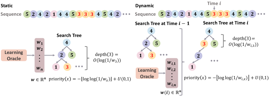
Figure 1: Sketch for static and dynamic learning augmented B-Trees. Since item 3 has a higher frequency around time $i$, the dynamic B-Trees adjust the priority accordingly.

Dynamic Learning Augmented B-Trees

We also consider the dynamic setting in which we continually update the priorities of a subset of items along with the sequence access. Rather than a fixed priority for each item, we allow the priorities to change as keys get accessed. The setting has a wide range of applications in the real world. For instance, consider accessing data in a relational database. A sequence of access will likely access related items one after another. So even if the entries themselves get accessed with fixed frequencies, the distribution of the next item to be accessed can be highly dependent on the set of recently accessed items. Consider the access sequence

$$4,2,3,4,5,2,3,4,5,2,3,4,5,1,4$$

versus the access sequence

$$5,2,4,2,1,4,4,5,3,3,3,4,5,4,2.$$

In both trees, the item $4$ is accessed the most frequently. So input dependent search trees should place it near the root. However, in the second sequence, the item $3$ is accessed three consecutive times around the middle. An algorithm that’s allowed to modify the tree dynamically can then modify the tree to place $3$ closer to root during those calls. An illustration of this is in Figure 1.

Thus, it is natural for the item priorities to vary as more items get accessed. We attempt to adapt Treaps and B-Treaps to this setting, specifically one where the predictions can change as more items get accessed.

Both Treaps and B-Treaps can handle updates to priorities efficiently. In particular, updating the priority of an element from $w_{x}$ to $w^{\prime}_{x}$ takes $O(|\log_{2}(w_{x}/w^{\prime}_{x})|)$ time for the Treap case and $O(|\log_{B}(w_{x}/w^{\prime}_{x})|)$ memory accesses for the B-Treap case. Denote $U(i)$ as the subset of items that update scores at time $i$ and $w_{i,j}$ as the score for item $j$ at time $i$. We show in Theorem 6.1 that the total cost for accessing the sequence $\mathbf{X}$ with the dynamic Treaps consists of two parts. The first part $O(n\log_{B}n+\sum_{i\in[m]}\log_{B}\frac{1}{w_{i,x(i)}})$ is the same as the static optimal bound and the second part $O(\sum_{i=2}^{m}\sum_{j\in U(i)}|\log_{B}\frac{w_{i,j}}{w_{i-1,j}}|)$ comes from updating scores. Hence, here is a trade-off between the costs of updating items and the benefits from the time-varying scores.

We study ways of designing composite priorities that cause this access cost to match known sequence-dependent access costs of binary trees (and their natural generalizations to B-Trees). Here, we focus on the working set bound, which says that the cost of accessing an item should be at most the logarithm of the number of distinct items until it gets accessed again. To obtain this bound, we propose a new composite priority named interval set priority, based on the number of distinct elements between two occurrences of the same item around accessed at step $i$. We give the guarantees for the dynamic Treaps with the interval set priority in Theorem 6.8. The dynamic B-Treaps further show the power of learning scores from data. While we have more data, we can quantify the dynamic environment in a more accurate way and thus improve the efficiency of the data structure.

Robustness to Prediction Inaccuracy

Finally, we provide some preliminary work on the robustness of our data structures to inaccuracies in prediction oracles.

In the static case, we can directly relate the overhead of having inaccurate frequency predictions to the KL divergences between the estimates and the true frequencies. This is because our composite priority can take any estimate, so plugging in the estimates $q_{x}$ gives that the overall access cost is exactly

$$m\cdot\sum_{x}q_{x}\log_{2}\left(\frac{1}{p_{x}}\right),$$

which is exactly the cross entropy between $\bm{p}$ and $\bm{q}$. On the other hand, the KL divergence between $\bm{p}$ and $\bm{q}$ is exactly the cross entropy minus the entropy of $\bm{p}$. So we get that the overhead of building the tree using noisy estimators $\bm{q}$ instead of the true frequencies $\bm{p}$ is exactly $m$ times the KL-divergence between $\bm{p}$ and $\bm{q}$. We formalize the argument above in Section 4.3.

In the online/dynamic setting, we incorporate notions from the analyses of recommender systems: each prediction can be treated as a recommendation/score of the item for future access. Recommender systems are widely studied in statistics, machine learning, and data mining. A variety of metrics have been proposed for them, and we follow the survey by Zangerle and Bauer [ZB22], specifically the notion of mean-average-error. In Theorem 6.9, we show that if the mean average error of the predicted priority vector is $\epsilon$, our learned B-Trees handle an access sequence with an additional overhead of $m\log_{B}(1+n\varepsilon/m)$.

3 Related Work

Learned Index Models

In recent years, there has been a surge of interest in integrating machine learning models into algorithm designs. A new field called Algorithms with Predictions [MV20] has garnered considerable attention, particularly in the use of machine learning models to predict input patterns to enhance performance. Examples of this approach include online graph algorithms with predictions [APT22], improved hashing-based methods such as Count-Min [CM05], and learning-augmented $k$-means clustering [EFSWZ21]. Practical oracles for predicting desired properties, such as predicting item frequencies in a data stream, have been demonstrated empirically [HIKV19, JLLRW20].

Capitalizing on the existence of oracles that predict the properties of upcoming accesses, researchers are now developing more efficient learning-augmented data structures. Index structures in database management systems are one significant application of learning-augmented data structures. One key challenge in this domain is to create search algorithms and data structures that are efficient and adaptive to data whose nature changes over time. This has spurred interest in incorporating machine learning techniques to improve traditional search tree performance.

The first study on learned index structures [KBCDP18] used deep-learning models to predict the position or existence of records as an alternative to the traditional B-Tree or hash index. However, this study focused only on the static case. Subsequent research [FV20, DMYWDLZCGK+20, WZCWCX21] introduced dynamic learned index structures with provably efficient time and space upper bounds for updates in the worst case. These structures outperformed traditional B-Trees in practice, but their theoretical guarantees were often trivial, with no clear connection between prediction quality and performance.

Beyond Worst-Case Analyses of Binary Trees

Binary trees are among the most ubiquitous pointer-based data structures. While schemes without re-balancing do obtain $O(\log_{2}{n})$ time bounds in the average case, their behavior degenerates to $\Omega(n)$ on natural access sequences such as $1,2,3,\ldots,n$. To remedy this, many tree balancing schemes with $O(\log_{2}{n})$ time worst-case guarantees have been proposed [AL63, GS78, CLRS09].

Creating binary trees optimal for their inputs has been studied since the 1970s. Given access frequencies, the static tree of optimal cost can be computed using dynamic programs or clever greedies [HT70, Meh75a, Yao82, KLR96]. However, the cost of such computations often exceeds the cost of invoking the tree. Therefore, a common goal is to obtain a tree whose cost is within a constant factor of the entropy of the data, multiple schemes do achieve this either on worst-case data [Meh75a], or when the input follows certain distributions [AM78].

A major disadvantage of static trees is that their cost on any permutation needs to be $\Omega(n\log_{2}{n})$. On the other hand, for the access sequence $1,2,3,\ldots,n$, repeatedly bringing the next accessed element to the root gives a lower cost $O(n)$. This prompted Allen and Munro to propose the notion of self-organizing binary search trees. This scheme was extended to splay trees by Sleator and Tarjan [ST85a]. Splay trees have been shown to obtain many improved cost bounds based on temporal and spatial locality [ST85a, CMSS00, Col00, Iac05]. In fact, they have been conjectured to have access costs with a constant factor of optimal on any access sequence [Iac13]. Much progress has been made towards showing this over the past two decades [DHIKP09, DS09, CCS19, BCIKL20]

From the perspective of designing learning-augmented data structures, the dynamic optimality conjecture almost goes contrary to the idea of incorporating predictors. It can be viewed as saying that learned advice do not offer gains beyond constant factors, at least in the binary search tree setting. Nonetheless, the notion of access sequence, as well as access-sequence-dependent bounds, provides useful starting points for developing prediction-dependent search trees in online settings. In this paper, we choose to focus on bounds based on temporal locality, specifically, the working set bound. This is for two reasons: the spatial locality of an element’s next access is significantly harder to describe compared to the time until the next access; and the current literature on spatial locality-based bounds, such as dynamic finger tends to be much more involved [CMSS00, Col00]. We believe an interesting direction for extending our composite scores is to obtain analogs of the unified bound [Iac01, BCDI07] for B-Trees.

B-Trees and External Memory Model

Parameterized B-Trees [BF03] have been studied to balance the runtime of read versus write operations, and several bounds have been shown with regard to the blocks of memory needed to be used during an operation. The optimality is discussed in both static and dynamic settings. Rosenberg and Snyder [RS81] compared the B-Tree with the minimum number of nodes (denoted as compact) with non-compact B-Trees and with time-optimal B-Trees. Bender et al. [BEHK16] considers keys have different sizes and gives a cache-oblivious static atomic-key B-Tree achieving the same asymptotic performance as the static B-Tree. When it comes to the dynamic setting, the trade-off between the cost of updates and accesses is widely studied [OCGO96, JNSSK97, JDO99, BGVW00, Yi12].

B-Treap were introduced by Golovin [Gol08, Gol09] as a way to give an efficient history-independent search tree in the external memory model. These studies revolved around obtaining $O(\log_{B}{n})$ worst-case costs that naturally generalize Treaps. Specifically, for sufficiently small $B$ (as compared to $n$), Golovin showed a worst-case depth of $O(\frac{1}{\alpha}\log_{B}n)$ with high probability, where $\alpha>0$ a parameter relating the limit on $B$ to $n$. The running time of this structure has recently been improved by Safavi [SS23] via a two-layer design.

The large node sizes of B-Trees interact naturally with the external memory model, where memory is accessed in blocks of size $B$ [BF03, Vit01]. The external memory model itself is widely used in data storage and retrieval [MA13], and has also been studied in conjunction with learned indices [FLV20]. There are a number of previous results discussing the trade-off between update and storage utilization  [Bro14, Bro17, FHM19].

4 Statically Optimal Binary Trees via Learning

In this section, we show that the widely taught Treap data structure can, with small modifications, achieves the static optimality conditions typically sought after in previous studies of learned index structures [LLW22, HIKV19].

Definition 4.1 (Treap, [AS89]).

Let $T$ be a Binary Search Tree over $[n]$ and ${\mathsf{priority}}\in\mathbb{R}^{n}$ be a priority assignment on $[n].$ We say $(T,{\mathsf{priority}})$ is a Treap if ${\mathsf{priority}}_{x}\leq{\mathsf{priority}}_{y}$ whenever $x$ is a descendent of $y$ in $T.$

Given a priority assignment ${\mathsf{priority}}$, one can construct a BST $T$ such that $(T,{\mathsf{priority}})$ is a Treap. $T$ is built as follows: Take any $x^{*}\in\operatorname*{arg\,max}_{x}{\mathsf{priority}}_{x}$ and build Treaps on $[1,x^{*}-1]$ and $[x^{*}+1,n]$ recursively using ${\mathsf{priority}}.$ Then, we just make $x^{*}$ the parent of both Treaps. Notice that if ${\mathsf{priority}}_{x}$’s are distinct, the resulting Treap is unique.

Observation 1.

Let ${\mathsf{priority}}\in\mathbb{R}^{n}$, which assigns each item $x$ to a unique priority. There is a unique BST $T$ such that $(T,{\mathsf{priority}})$ is a Treap.

From now on, we always assume that ${\mathsf{priority}}$ has distinct values. Therefore, when ${\mathsf{priority}}$ is clear from the context, the term Treap is referred to the unique BST $T.$ For each node $x\in[n]$, we use $0pt(x)$ to denote its depth in $T.$

Given any two items $x,y\in[n]$, one can determine whether $x$ is an ancestor of $y$ in the Treap without traversing the tree. In particular, $x$ is an ancestor of $y$ if $x$’s priority is the largest among items $[x,y].$

Observation 2.

Given any $x,y\in[n]$, $x$ is an ancestor of $y$ if and only if ${\mathsf{priority}}_{x}=\max_{z\in[x,y]}{\mathsf{priority}}_{z}$.

A classical result of [AS89] states that if priorities are randomly assigned, the depth of the Treap cannot be too large.

Lemma 4.2 ([AS89]).

Let $U(0,1)$ be the uniform distribution over the real interval $[0,1].$ If ${\mathsf{priority}}\sim U(0,1)^{n}$, each Treap node $x$ has depth $\Theta(\log_{2}n)$ with high probability.

Proof.

Notice that $0pt(x)$, the depth of item $x$ in the Treap, is the number of ancestors of $x$ in the Treap. Linearity of expectation yields

$$\mathbb{E}[0pt(x)] =\sum_{y\in[n]}\mathbb{E}[\text{$1$ if $y$ is an ancestor of $x$ or $0$}]$$

$$=\sum_{y\in[n]}\Pr\left(\text{$y$ is an ancestor of $x$}\right)$$

$$=\sum_{y\in[n]}\Pr\left({\mathsf{priority}}_{y}=\max_{z\in[x,y]}{\mathsf{priority}}_{z}\right)=\sum_{y\in[n]}\frac{1}{\left|x-y+1\right|}=\Theta(\log_{2}n).$$

∎

Treaps can be made dynamic and support operations such as insertions and deletions.

Lemma 4.3 ([AS89]).

Given a Treap $T$ and some item $x\in[n]$, $x$ can be inserted to or deleted from $T$ in $O(0pt(x))$-time.

4.1 Learning-Augmented Treaps

In this section, we present the construction of composite priorities and prove the following theorem.

Theorem 4.4 (Learning-Augmented Treap via Composite Priorities).

Denote $\bm{w}=(w_{1},\cdots,w_{n})\in\mathbb{R}^{n}$ as a score associated with each item in $[n]$ such that $\|\bm{w}\|_{1}=O(1)$. Consider the following priority assignment of each item:

$${\mathsf{priority}}_{x}\stackrel{{\scriptstyle\mathrm{\scriptscriptstyle def}}}{{=}}-\left\lfloor\log_{2}\log_{2}\frac{1}{w_{x}}\right\rfloor+\delta_{x},~{}\delta_{x}\sim U(0,1),~{}x\in[n]$$

where $\delta_{x}$ is drawn uniformly from $(0,1)$ via a $11$-wise independent hash function. The depth of any item $x\in[n]$ is $O(\log_{2}(1/w_{x}))$ in expectation.

Remark 4.5.

The data structure supports insertions and deletions naturally. Suppose the score of some node $x$ changes from $w$ to $w^{\prime}$, the Treap can be maintained with $O(|\log_{2}(w^{\prime}/w)|)$ rotations in expectation.

For any item $x\in[n]$, we define $x$’s tier, $\tau_{x}$, to be the integral part of its priority, i.e.,

$$\tau_{x}\stackrel{{\scriptstyle\mathrm{\scriptscriptstyle def}}}{{=}}\left\lfloor\log_{2}\log_{2}\frac{1}{w_{x}}\right\rfloor=-\lfloor{\mathsf{priority}}_{x}\rfloor.$$ (1)

In addition, we define $S_{t}=\left\{x\in[n]~{}\middle|~{}\tau_{x}=t\right\}$ for any $t.$ For simplicity, we assume that $\tau_{x}\geq 0$ for any $x$ WLOG. This is because $\tau_{x}<0$ implies $w_{x}=\Omega(1)$ which can hold for only a constant number of items. We can always make them stay at the top of the Treap. This only increases the depths of others by a constant.

Let $x$ start at any node and approach the root. The tier $\tau_{x}$ decreases. In other words, the smaller the $\tau_{x}$, the smaller the depth $0pt(x).$ However, there may be many items of the same tier $\tau_{x}.$ The ties are broken randomly due to the random offset $\delta_{x}\sim U(0,1)$. Similar to the ordinary Treaps, where every item has the same tier, any item has $O(\log_{2}|S_{t}|)$ ancestors with tier $w$ in expectation. To prove the desired bound, we will show that $\log_{2}|S_{t}|=O(2^{t}).$ Since each ancestor of item $x$ has weight at most $\tau_{x}$, the expected depth $\mathbb{E}[0pt(x)]$ can be bound by $O(2^{0}+2^{1}+\ldots+2^{\tau_{x}})=O(2^{\tau_{x}})=O(\log_{2}(1/w_{x})).$ First, let us bound the size of each $S_{w}.$

Lemma 4.6.

For any non-negative integer $t\geq 0$, $\left|S_{t}\right|=O(2^{O(2^{t})}).$

Proof.

Observe that $x\in S_{t}$ if and only if

$$t\leq\log_{2}\log_{2}(1/w_{x})\leq t+1,\text{ and }2^{2^{t}}\leq\frac{1}{w_{x}}\leq 2^{2^{t+1}}.$$

However, there are only $O({\mathrm{poly}}(2^{2^{t+1}}))=O(2^{O(2^{t})})$ such items because the total score $\|\bm{w}\|_{1}=O(1).$ ∎

Next, we bound the expected number of ancestors of item $x$ in $S_{w},w\leq w_{x}.$

Lemma 4.7.

Let $x\in[n]$ be any item and $t\leq\tau_{x}$ be a non-negative integer. The expected number of ancestors of $x$ in $S_{t}$ is at most $O(\log_{2}|S_{t}|).$

Proof.

First, we show that any $y\in S_{t}$ is an ancestor of $x$ with probability no more than $1/|S_{t}\cap[x,y]|.$ 2 says that $y$ must have the largest priority among items $[x,y].$ Thus, a necessary condition for $y$ being $x$’s ancestor is that $y$ has the largest priority among items in $S_{t}\cap[x,y].$ However, priorities of items in $S_{t}\cap[x,y]$ are i.i.d. random variables of the form $-t+U(0,1).$ Thus, the probability that ${\mathsf{priority}}_{y}$ is the largest among them is $1/|S_{t}\cap[x,y]|.$

Now, we can bound the expected number of ancestors of $x$ in $S_{t}$ as follows:

$$\mathbb{E}[\text{number of ancestors of $x$ in $S_{t}$}] =\sum_{y\in S_{t}}\Pr\left(\text{$y$ is an ancestor of $x$}\right)$$

$$\leq\sum_{y\in S_{t}}\frac{1}{\left|S_{t}\cap[x,y]\right|}$$

$$\leq 2\cdot\sum_{u=1}^{|S_{t}|}\frac{1}{u}=O(\log_{2}|S_{t}|),$$

where the second inequality comes from the fact that for a fixed value of $u$, there are at most two items $y\in S_{t}$ with $|S_{t}\cap[x,y]|=u$ (one with $y\leq x$, the other with $y>x$). ∎

Now we are ready to prove Theorem 4.4.

Proof of Theorem 4.4.

Let $x\in[n]$ be any item. Linearity of expectation yields

$$\mathbb{E}[0pt(x)] =\sum_{t=0}^{\tau_{x}}\mathbb{E}[\text{number of ancestors of $x$ in $S_{t}$}]$$

$$\underset{\text{\lx@cref{creftypecap~refnum}{lemma:scoreDepthPerBucket}}}{\lesssim}\sum_{t=0}^{\tau_{x}}\log_{2}\left|S_{t}\right|$$

$$\underset{\text{\lx@cref{creftypecap~refnum}{lemma:scoreBucketSize}}}{\lesssim}\sum_{t=0}^{\tau_{x}}2^{t}\lesssim 2^{\tau_{x}}.$$

We conclude the proof by observing that

$$\tau_{x}\leq\log_{2}\log_{2}\frac{1}{w_{x}}\leq\tau_{x}+1,\text{ and }2^{\tau_{x}}\leq\log_{2}\frac{1}{w_{x}}.$$

∎

4.2 Static Optimality

We present a priority assignment for constructing statically optimal Treaps given item frequencies. Given any access sequence $\mathbf{X}=(x(1),\ldots,x(m))$, we define $f_{x}$ for any item $x$, to be its frequency in $\mathbf{X}$, i.e. $f_{x}\coloneqq|\left\{i\in[m]~{}\middle|~{}x(i)=x\right\}|,x\in[n].$ For simplicity, we assume that every item is accessed at least once, i.e., $f_{x}\geq 1,x\in[n].$ We prove the following technical result which is a simple application of Theorem 4.4:

Theorem 4.8 (Static Optimality).

For any item $x\in[n]$, we set its priority as

$${\mathsf{priority}}_{x}\coloneqq-\left\lfloor\log_{2}\log_{2}\frac{m}{f_{x}}\right\rfloor+\delta_{x},\delta_{x}\sim U(0,1).$$

In the corresponding Treap, each node $x$ has expected depth $O(\log_{2}(m/f_{x})).$ Therefore, the total time for processing the access sequence is $O(\sum_{x}f_{x}\log_{2}(m/f_{x}))$, which matches the performance of the optimal static BSTs up to a constant factor.

Proof.

Given item frequencies $\bm{f}$, we define the following $\bm{w}$ assignment:

$$w_{x}\coloneqq\frac{f_{x}}{m},~{}x\in[n].$$ (2)

One can verify that $\|\bm{w}\|_{1}=O(1)$, therefore Theorem 4.4 yields that the expected depth of each item $x$ is $O(\log_{2}(m/f_{x})).$ ∎

4.3 Robustness Guarantees

In practice, one could only estimates $q_{x}\approx p_{x}=f_{x}/m,x\in[n].$ A natural question arises: how does the estimation error affect the performance? In this section, we analyze the drawback in performance given estimation errors. As a result, we will show that our Learning-Augmented Treaps are robust against noise and errors.

For each item $x\in[n]$, define $p_{x}=f_{x}/m$ to be the relative frequency of item $x.$ One can view $\bm{p}$ as a probability distribution over $[n]$. Using the notion of entropy, one can express Theorem 4.8 as the following claim:

Definition 4.9 (Entropy).

Given a probability distribution $\bm{p}$ over $[n]$, define its Entropy as ${\mathrm{Ent}}(\bm{p})\coloneqq\sum_{x}p_{x}\log_{2}(1/p_{x})=\mathbb{E}_{x\sim\bm{p}}[\log_{2}(1/p_{x})].$

Corollary 4.10.

In Theorem 4.8, the expected depth of each item $x$ is $O(\log_{2}(1/p_{x}))$ and the expected total cost is $O(m\cdot{\mathrm{Ent}}(\bm{p}))$, where ${\mathrm{Ent}}(\bm{p})=\sum_{x}p_{x}\log_{2}(1/p_{x})$ measures the entropy of the distribution $\bm{p}.$

The appearance of entropy in the runtime bound suggests that some more related notations would appear in the analysis. Let us present several related notions.

Definition 4.11 (Cross Entropy).

Given two distributions $\bm{p},\bm{q}$ over $[n]$, define its Cross Entropy as ${\mathrm{Ent}}(\bm{p},\bm{q})\coloneqq\sum_{x}p_{x}\log_{2}(1/q_{x})=\mathbb{E}_{x\sim\bm{p}}[\log_{2}(1/q_{x})].$

Definition 4.12 (KL Divergence).

Given two distributions $\bm{p},\bm{q}$ over $[n]$, define its KL Divergence as ${\mathrm{D_{KL}}}(\bm{p},\bm{q})={\mathrm{Ent}}(\bm{p},\bm{q})-{\mathrm{Ent}}(\bm{p})=\sum_{x}p_{x}\log_{2}(p_{x}/q_{x}).$

First, we analyze the run time given frequency estimations $\bm{q}.$

Theorem 4.13.

Given an estimation $\bm{q}$ on the relative frequencies $\bm{p}.$ For any item $x\in[n]$, we draw a random number $\delta_{x}\sim U(0,1)$ and set its priority as

$${\mathsf{priority}}_{x}\coloneqq-\left\lfloor\log_{2}\log_{2}\frac{1}{q_{x}}\right\rfloor+\delta_{x}.$$

In the corresponding Treap, each node $x$ has expected depth $O(\log_{2}(1/q_{x})).$ Therefore, the total time for processing the access sequence is $O(m\cdot{\mathrm{Ent}}(\bm{p},\bm{q}))$.

Proof.

Define score $s(x)=1/q_{x}$ for each item $x\in[n].$ Clearly, $s$ is smooth and we can apply Theorem 4.4 to prove the bound on the expected depths. The total time for processing the access sequence is, by definition,

$$O\left(\sum_{x\in[n]}f_{x}\log_{2}\frac{1}{q_{x}}\right)=O\left(m\cdot\sum_{x\in[n]}p_{x}\log_{2}\frac{1}{q_{x}}\right)=O\left(m\cdot{\mathrm{Ent}}(\bm{p},\bm{q})\right).$$

∎

Using the theorem, one can relate the drawback in the performance given $\bm{q}$ in terms of KL Divergence.

Corollary 4.14.

In the setting of Theorem 4.13, the extra time spent compared to using $\bm{p}$ to build the Treap is $O(m\cdot{\mathrm{D_{KL}}}(p,q))$ in expectation.

4.4 Analysis of Other Variations

We discuss two different priority assignments. For each assignment, we construct an input distribution that creates a larger expected depth than Theorem 4.8. We define the distribution $\bm{p}$ as $p_{x}=f_{x}/m,x\in[n]$.

The first priority assignment is used in [LLW22]. They assign priorities according to $p_{x}$ entirely, i.e., ${\mathsf{priority}}_{x}=p_{x},x\in[n].$ Assuming that items are ordered randomly, and $\bm{p}$ is a Zipfian distribution, [LLW22] shows Static Optimality. However, it does not generally hold, and the expected access cost could be $\Omega(n)$.

Theorem 4.15.

Consider the priority assignment that assigns the priority of each item to be ${\mathsf{priority}}_{x}\coloneqq p_{x},x\in[n].$ There is a distribution $\bm{p}$ over $[n]$ such that the expected access time, $\mathbb{E}_{x\sim\bm{p}}[0pt(x)]=\Omega(n).$

Proof.

We define for each item $x$, $p_{x}\coloneqq\frac{2(n-x+1)}{n(n+1)}.$ One could easily verify that $\bm{p}$ is a distribution over $[n].$ In addition, the smaller the item $x$, the larger the priority ${\mathsf{priority}}_{x}.$ Thus, by the definition of Treaps, item $x$ has depth $x.$ The expected access time of $x$ sampled from $\bm{p}$ can be lower bounded as follows:

$$\mathbb{E}_{x\sim\bm{p}}[0pt(x)] =\sum_{x\in[n]}p_{x}\cdot 0pt(x)$$

$$=\sum_{x\in[n]}\frac{2(n-x+1)}{n(n+1)}\cdot x$$

$$=\frac{2}{n(n+1)}\sum_{x\in[n]}x(n-x+1)$$

$$\gtrsim\frac{2}{n(n+1)}\cdot n^{3}\gtrsim n.$$

∎

Next, we consider a very similar assignment to ours.

Theorem 4.16.

Consider the following priority assignment that sets the priority of each node $x$ as ${\mathsf{priority}}_{x}\coloneqq-\lfloor\log_{2}1/p_{x}\rfloor+\delta_{x},\delta_{x}\sim U(0,1)$. There is a distribution $\bm{p}$ over $[n]$ such that the expected access time, $\mathbb{E}_{x\sim\bm{p}}[0pt(x)]=\Omega(\log_{2}^{2}n).$

Proof.

We assume WLOG that $n$ is an even power of $2.$ Define $K=\frac{1}{2}\log_{2}n.$ We partition $[n]$ into $K+1$ segments $S_{1},\ldots,S_{K},S_{K+1}\subseteq[n]$. For $i=1,2,\ldots,K$, we add $2^{1-i}\cdot n/K$ elements to $S_{i}$. Thus, $S_{1}$ has $n/K$ elements, $S_{2}$ has $n/2K$, and $S_{K}$ has $\sqrt{n}/K$ elements. The rest are moved to $S_{K+1}.$

Now, we can define the distribution $\bm{p}$. Elements in $S_{K+1}$ have zero-mass. For $i=1,2,\ldots,K$, elements in $S_{i}$ has probability mass $2^{i-1}/n.$ One can directly verify that $\bm{p}$ is indeed a probability distribution over $[n].$

In the Treap with the given priority assignment, $S_{i}$ forms a subtree of expected height $\Omega(\log_{2}n)$ since $\left|S_{i}\right|\geq n^{1/3}$ for any $i=1,2,\ldots,K$ (Lemma 4.2). In addition, every element of $S_{i}$ passes through $S_{i+1},S_{i+2},\ldots,S_{K}$ on its way to the root since they have strictly larger priorities. Therefore, the expected depth of element $x\in S_{i}$ is $\Omega((K-i)\log_{2}n).$ One can lower bound the expected access time (which is the expected depth) as:

$$\mathbb{E}_{x\sim\bm{p}}[0pt(x)] \gtrsim\sum_{i=1}^{K}\sum_{x\in S_{i}}p_{x}\cdot(K-i)\cdot\log_{2}n$$

$$=\sum_{i=1}^{K}\bm{p}(S_{i})\cdot(K-i)\cdot\log_{2}n$$

$$=\sum_{i=1}^{K}\frac{1}{K}\cdot(K-i)\cdot\log_{2}n\gtrsim K\log_{2}n\gtrsim\log_{2}^{2}n,$$

where we use $\bm{p}(S_{i})=|S_{i}|\cdot 2^{i-1}/n=1/K$ and $K=\Theta(\log_{2}n).$ That is, the expected access time is at least $\Omega(\log_{2}^{2}n)$. ∎

5 Learning-Augmented B-Trees: Static Optimality

We now extend the ideas above, specifically the composite priority notions, to B-Trees in the External Memory Model, and also obtain static optimality in this model. This model is also the core of our analyses in the online settings in the next section (Section 6).

We first formalize this extension by incorporating our composite priorities with the B-Treap data structure from [Gol09] and introducing offsets in priorities.

5.1 Learning-Augmented B-Treaps

Lemma 5.1 (B-Treap, [Gol09]).

Given the unique binary Treap $(T,{{\mathsf{priority}}_{x}})$ over the set of items $[n]$ with their associated priorities, and a target branching factor $B=\Omega(\ln^{1/(1-\alpha)}n)$ for some $\alpha>0$. Assuming ${{\mathsf{priority}}_{x}}$ are drawn uniformly from $(0,1)$ using an 11-wise independent hash function, we can maintain a B-Tree $T^{B}$, called the B-Treap, uniquely defined by $T$. This allows operations such as Lookup, Insert, and Delete of an item to touch $O(\frac{1}{\alpha}\log_{B}n)$ nodes in $T^{B}$ in expectation.

In particular, if $B=O(n^{1/2-\delta})$ for some $\delta>0$, all above performance guarantees hold with high probability.

The main technical theorem is the following:

Theorem 5.2 (Learning-Augmented B-Treap via Composite Priorities).

Denote $\bm{w}=(w_{1},\cdots,w_{n})\in\mathbb{R}^{n}$ as a score associated with each element of $[n]$ such that $\|\bm{w}\|_{1}=O(1)$ and a branching factor $B=\Omega(\ln^{1/(1-\alpha)}n)$, there is a randomized data structure that maintains a B-Tree $T^{B}$ over $U$ such that

1. Each item $x$ has expected depth $O(\frac{1}{\alpha}\log_{B}(1/w_{x})).$

2. Insertion or deletion of item $x$ into/from $T$ touches $O(\frac{1}{\alpha}\log_{B}(1/w_{x}))$ nodes in $T^{B}$ in expectation.

3. Updating the weight of item $x$ from $w$ to $w^{\prime}$ touches $O(\frac{1}{\alpha}|\log_{B}(w^{\prime}/w)|)$ nodes in $T^{B}$ in expectation.

We consider the following priority assignment scheme: For any $x$ and its corresponding score $w_{x}$, we always maintain:

$${\mathsf{priority}}_{x}\coloneqq-\lfloor\log_{4}\log_{B}\frac{1}{w_{x}}\rfloor+\delta,~{}\delta\sim U(0,1).$$

In addition, if $B=O(n^{1/2-\delta})$ for some $\delta>0$, all above performance guarantees hold with high probability $1-\delta$.

The learning-augmented B-Treap is created by applying Lemma 5.1 to a partition of the binary Treap $T$. Each item $x$ has a priority in the binary Treap $T$, defined as:

$${\mathsf{priority}}_{x}=-\left\lfloor\log_{4}\log_{B}\frac{1}{w_{x}}\right\rfloor+\delta_{x},\delta_{x}\sim U(0,1),\mathrm{\text{ for all }}x\in U$$ (3)

We then partition the binary Treap $T$ based on each item’s tier. The tier of an item is defined as the absolute value of the integral part of its priority, i.e., $\tau_{x}\stackrel{{\scriptstyle\mathrm{\scriptscriptstyle def}}}{{=}}\lfloor\log_{4}\log_{B}(1/w_{x})\rfloor$.

Proof of Theorem 5.2.

To formally construct and maintain $T^{B}$, we follow these steps:

1. Start with a binary Treap $(T,{{\mathsf{priority}}_{x}})$ with priorities defined using equation (3).

2. Decompose $T$ into sub-trees based on each item’s tier, resulting in a set of maximal sub-trees with items sharing the same tier.

3. For each $T_{i}$, apply Lemma 5.1 to maintain a B-Treap $T^{B}_{i}$.

4. Combine all the B-Treaps into a single B-Tree, such that the parent of $\mathsf{root}(T^{B}_{i})$ is the B-Tree node containing the parent of $\mathsf{root}(T_{i})$.

Now, let’s analyze the depth of each item $x$. Keep in mind that any item $y$ in the same B-Tree node shares the same tier. Therefore, we can define the tier of each B-Tree node as the tier of its items.

Suppose $x_{1},x_{2},\ldots$ are the B-Tree nodes we encounter until we reach $x$. The tiers of these nodes are in non-increasing order, that is, $\tau_{x_{i}}\geq\tau_{x_{i+1}}$ for any $i$. We’ll define $C_{t}$ as the number of items of tier $t$ for any $t$. As per the definition (refer to equation (3)), we have:

$$C_{t}=O(B^{4^{t}}),\mathrm{\text{ for all }}t$$

Using Lemma 5.1 and the fact that $B=O(C_{t}^{1/4}),t\geq 1$, we find that the number of nodes among ${x_{i}}$ of tier $t$ is $O(\frac{1}{\alpha}\log_{B}C_{t})=O(4^{t}/\alpha)$ with high probability. As a result, the number of nodes touched until reaching $x$ is, with high probability:

$$\sum_{t=0}^{\tau_{x}}O(4^{t}/\alpha)=O(4^{\tau_{x}}/\alpha)=O\left(\frac{1}{\alpha}\log_{B}\frac{1}{w_{x}}\right)$$

This analysis is also applicable when performing Lookup, Insert, and Delete operations on item $x$.

The number of nodes touched when updating an item’s weight can be derived from first deleting and then inserting the item.

∎

We also show that this mechanism is robust to noisy predictions of item frequencies. Let $x(1),x(2),\ldots,x(m)$ represent an access sequence of length $m$. We define the density of each item $x$ as follows:

$$p_{x}\stackrel{{\scriptstyle\mathrm{\scriptscriptstyle def}}}{{=}}\frac{|\left\{i\in[m]~{}\middle|~{}x(i)=x\right\}|}{m}$$

Note that $\bm{p}\in\mathbb{R}^{n}_{+}$ defines a probability distribution over all items. A static B-Tree is statically optimal if the depth of each item $x$ is:

$$0pt(x)=O\left(\log_{B}\frac{1}{p_{x}}\right),\mathrm{\text{ for all }}x\in[n]$$

5.2 Static Optimality

If we are given the density $\bm{p}$, we can achieve Static Optimality using Theorem 5.2 with weights $w_{x}\stackrel{{\scriptstyle\mathrm{\scriptscriptstyle def}}}{{=}}p_{x}.$

Lemma 5.3 (Static Optimality for B-Treaps).

Given the density $\bm{p}$ of each item over the access sequence $x(1),x(2),\ldots,x(m)$, and a branching factor $B=\Omega(\ln^{1.1}n)$, there exists a randomized data structure that maintains a B-Tree $T^{B}$ over $[n]$ such that each item $x$ has an expected depth of $O(\log_{B}1/p_{x})$. That is, $T^{B}$ achieves Static Optimality (SO), meaning the total number of nodes touched is $O(OPT^{\text{static}}_{B})$ in expectation, where:

$$OPT^{\text{static}}_{B}\stackrel{{\scriptstyle\mathrm{\scriptscriptstyle def}}}{{=}}m\cdot\sum_{x\in[n]}p_{x}\log_{B}\frac{1}{p_{x}}$$ (4)

Furthermore, if $B=O(n^{1/2-\delta})$ for some $\delta>0$, all above performance guarantees hold with high probability.

In practice, we would not have access to the exact density $\bm{p}$ but an inaccurate prediction $\widetilde{\bm{p}}\approx\bm{p}$. We assume WLOG that $|p(x)|,|\widetilde{p}(x)|\geq\Theta(1/n)$. Nevertheless, we will show that B-Treap performance is robust to the error. Specifically, we analyze the performance under various notions of error in the prediction. The notions listed here are the ones used for learning discrete distributions (refer to [Can20] for a comprehensive discussion).

Corollary 5.4 (Kullback—Leibler (KL) Divergence).

If we are given a density prediction $\widetilde{\bm{p}}$ such that $d_{KL}(\bm{p};\widetilde{\bm{p}})=\sum_{x}p_{x}\ln(p_{x}/\widetilde{\bm{p}}_{x})\leq\varepsilon$, the total number of touched nodes is

$$O\left(OPT^{\text{static}}_{B}+\frac{\varepsilon m}{\ln B}\right)$$

Proof.

Given the inaccurate prediction $\widetilde{\bm{p}}$, the total number of touched nodes in $T^{B}$ is

$$O\left(\sum_{x}m\cdot p_{x}\log_{B}\frac{1}{\widetilde{\bm{p}}_{x}}\right)=O\left(\sum_{x}m\cdot p_{x}\log_{B}\frac{1}{p_{x}}+m\cdot\sum_{x}p_{x}\log_{B}\frac{p_{x}}{\widetilde{\bm{p}}_{x}}\right)=O(OPT^{\text{static}}_{B}+m\frac{d_{KL}(\bm{p};\widetilde{\bm{p}})}{\ln B})$$

∎

Corollary 5.5 ($\chi^{2}$).

If we are given a density prediction $\widetilde{\bm{p}}$ such that $\chi^{2}(\bm{p};\widetilde{\bm{p}})=\sum_{x}(p_{x}-\widetilde{\bm{p}}_{x})^{2}/\widetilde{\bm{p}}_{x}\leq\varepsilon$, the total number of touched nodes is

$$O\left(OPT^{\text{static}}_{B}+\frac{\varepsilon m}{\ln B}\right)$$

Proof.

The corollary follows from Corollary 5.5 and the fact $d_{KL}(\bm{p};\widetilde{\bm{p}})\leq\chi^{2}(\bm{p};\widetilde{\bm{p}})\leq\varepsilon.$ ∎

Corollary 5.6 ($L_{\infty}$ Distance).

If we are given a density prediction $\widetilde{\bm{p}}$ such that $\|\bm{p}-\widetilde{\bm{p}}\|_{\infty}\leq\varepsilon$, the total number of touched nodes is

$$O\left(OPT^{\text{static}}_{B}+m\log_{B}(1+\varepsilon n)\right)$$

Proof.

For item $x$ with its marginal probability smaller than $1/1000n$, its expected depth in the B-Treap is $O(\log_{B}n)$ using either $p_{x}$ or $\widetilde{\bm{p}}_{x}$ as its score. If item $x$’s marginal probability is at least $1/1000n$, the $L_{\infty}$ distance implies that

$$\frac{p_{x}}{\widetilde{p}_{x}}=1+\frac{p_{x}-\widetilde{p}_{x}}{\widetilde{p}_{x}}\leq 1+\frac{\varepsilon}{1/(1000n)}=1+1000(1+\varepsilon n)$$

Therefore, item $x$’s expected depth in the B-Treap with score $\widetilde{\bm{p}}$ is roughly

$$O\left(\log_{B}\frac{1}{p_{x}}+\log_{B}\frac{p_{x}}{\widetilde{\bm{p}}_{x}}\right)\leq O\left(\log_{B}\frac{1}{p_{x}}+\log_{B}(1+\varepsilon n)\right)$$

The corollary follows. ∎

Corollary 5.7 ($L_{2}$ Distance).

If we are given a density prediction $\widetilde{\bm{p}}$ such that $\|\bm{p}-\widetilde{\bm{p}}\|_{2}\leq\varepsilon$, the total number of touched nodes is

$$O\left(OPT^{\text{static}}_{B}+m\log_{B}(1+\varepsilon n)\right)$$

Proof.

This claim follows from Corollary 5.6 and the fact $\|\bm{p}-\widetilde{\bm{p}}\|_{\infty}\leq\|\bm{p}-\widetilde{\bm{p}}\|_{2}\leq\varepsilon.$ ∎

Corollary 5.8 (Total Variation).

If we are given a density prediction $\widetilde{\bm{p}}$ such that $d_{TV}(\bm{p},\widetilde{\bm{p}})=0.5\|\bm{p}-\widetilde{\bm{p}}\|_{1}\leq\varepsilon$, the total number of touched nodes is

$$O\left(OPT^{\text{static}}_{B}+m\log_{B}(1+\varepsilon n)\right)$$

Proof.

This claim follows from Corollary 5.6 and the fact $\|\bm{p}-\widetilde{\bm{p}}\|_{\infty}\leq\|\bm{p}-\widetilde{\bm{p}}\|_{1}\leq 2\varepsilon.$ ∎

Corollary 5.9 (Hellinger Distance).

If we are given a density prediction $\widetilde{\bm{p}}$ such that $d_{H}(\bm{p},\widetilde{\bm{p}})=0.5\|\sqrt{\bm{p}}-\sqrt{\widetilde{\bm{p}}}\|_{2}\leq\varepsilon$, the total number of touched nodes is

$$O\left(OPT^{\text{static}}_{B}+m\log_{B}(1+\varepsilon n)\right)$$

Proof.

This claim follows from Corollary 5.6 and the fact $\|\bm{p}-\widetilde{\bm{p}}\|_{\infty}\leq 2\sqrt{2}d_{H}(\bm{p},\widetilde{\bm{p}})\leq 2\sqrt{2}\varepsilon.$ ∎

6 Dynamic Learning-Augmented B-Trees

In this section, we first construct the dynamic B-Treaps and give the guarantees when we have access to the real-time priorities for each item. Then we show that our Treaps are robust to the estimation error of the time-varying priorities. Finally, we consider a specific score that is highly related to the working-set theorem [ST85].

6.1 General Results for Dynamic B-Trees

Dynamic B-Trees Setting.

Given $n$ items, denoted as $[n]=\{1,\cdots,n\}$, and a sequence of access sequence $\mathbf{X}=(x(1),\ldots,x(m))$, where $x(i)\in[n]$. At time $i\in[m]$, there exists some time-dependent priority $w_{ij}$ for each item $j,j\in[n]$. Denote $\bm{w}(i)=(w_{i,1},\cdots,w_{i,n})\in\mathbb{R}^{n}$ as the time-varying priority vector, and $\widetilde{\bm{w}}(i)=(\widetilde{w}_{i,1},\cdots,\widetilde{w}_{i,n})$ as its estimator. We aim to maintain a data structure that achieves a small total cost for accessing the sequence $S$ given inaccurate score estimators $\widetilde{\bm{w}}_{i},i\in[m]$.

We first show the guarantees when we are given the accurate time-varying priorities $\bm{w}(i),i\in[m]$ in Theorem 6.1. The proof is an application of Theorem 5.2, where the priority function dynamically changes as time goes on, rather than the Static Optimality case where the priority is fixed beforehand. Here for any vector $\bm{w}$, we write $\log\bm{w}$ as the vector taking the element-wise $\log$ on $\bm{w}$.

Theorem 6.1 (Dynamic B-Treap with Given Priorities).

Given the time-varying priority vector $\bm{w}(i)\in\mathbb{R}^{n},i\in[m]$ satisfying $\|\bm{w}(i)\|_{1}=O(1)$ and a branching factor $B=\Omega(\ln^{1.1}n)$, there is a randomized data structure that maintains a B-Tree $T^{B}$ over $[n]$ such that when accessing the item $x(i)$ at time $i$, the expected depth of item $x(i)$ is $O(\log_{B}\frac{1}{w_{i,x(i)}}).$ The expected total cost for processing the whole access sequence $\mathbf{X}$ is

$$\mathsf{cost}(\mathbf{X},\bm{w})=O\left(n\log_{B}n+\sum_{i=1}^{m}\log_{B}\frac{1}{w_{i,x(i)}}+\sum_{i=2}^{m}\left\lVert\log_{B}\bm{w}(i)-\log_{B}\bm{w}({i-1})\right\rVert_{1}\right).$$

Furthermore, for $\delta>0$, by setting $B=O(n^{1/2-\delta})$, the guarantees hold with probability $1-\delta$.

Proof.

Initially, we set the priority for all items to be $1$, and insert all items into the Treap. For any time $i\in[n]$, for $j\in[n]$ such that $w_{i-1,j}\neq w_{i,j}$, we set

$${\mathsf{priority}}^{(i)}_{j}\coloneqq-\lfloor\log_{4}\log_{B}\frac{1}{w_{i,j}}\rfloor+\delta_{ij},\delta_{ij}\sim U(0,1).$$

Since $\|w(i)\|_{1}=O(1),i\in[m]$, by Theorem 5.2, the expected depth of item $s(i)$ is $O(\log_{B}\frac{1}{w_{i,x(i)}})$. The total cost for processing the sequence consists of both accessing $x(i)$ and updating the priorities. The expected total cost for all the accesses is

$$O\left(\sum_{i=1}^{m}\log_{B}\frac{1}{w_{i,x(i)}}\right).$$

Then we will calculate the cost to update the Treap. Updating the priority of $j$ from $w_{i-1,j}$ to $w_{i,j}$ has cost $O(|\log_{B}(w_{i-1,j}/w_{i,j})|)$ Hence we can bound the expected total cost for maintaining the Treap by

$$O\left(n\log_{B}n+\sum_{i=2}^{m}\sum_{j=1}^{n}\left|\log_{B}\frac{w_{i-1,j}}{w_{i,j}}\right|\right).$$

Together the expected total cost is

$$O\left(n\log_{B}n+\sum_{i=1}^{m}\log_{B}\frac{1}{w_{i,x(i)}}+\sum_{i=2}^{m}\left\lVert\log_{B}\bm{w}(i)-\log_{B}\bm{w}(i-1)\right\rVert_{1}\right).$$

The high probability bound follows similarly as Theorem 5.2. ∎

Next, we will give the guarantees for the dynamic B-Treaps with predicted priorities learned by a machine learning oracle.

Theorem 6.2 (Dynamic B-Treap with Predicted Scores).

Given the time-varying priority vector $\bm{w}(i)\in\mathbb{R}^{n},i\in[m]$ and its estimator $\widetilde{\bm{w}}(i)\in\mathbb{R}_{+}^{n}$ satisfying $\|\widetilde{\bm{w}}(i)\|_{1}=O(1)$, $\widetilde{w}_{i,j}\geq 1/{\mathrm{poly}}(n)$. Denote $\varepsilon_{i,j}=\widetilde{w}_{i,j}-w_{i,j}$. Then for a branching factor $B=\Omega(\ln^{1.1}n)$, there is a randomized data structure that maintains a B-Tree $T^{B}$ over $[n]$ such that when accessing $x_{s(i)}$ at time $i$, the expected depth of item $x(i)$ is $O\left(\log_{B}\left(\frac{1}{w_{i,x(i)}}\left(1+n|\varepsilon_{i,x(i)}|\right)\right)\right).$ The expected total cost for processing the whole access sequence $\mathbf{X}$ given the predicted priority $\widetilde{\bm{w}}$ is

$$\mathsf{cost}(\mathbf{X},\widetilde{\bm{w}})=O\left(n\log_{B}n+\sum_{i=1}^{m}\log_{B}\left(\frac{1}{w_{i,x(i)}}\left(1+n|\varepsilon_{i,x(i)}|\right)\right)+\sum_{i=2}^{m}\left\lVert\log_{B}\widetilde{\bm{w}}(i)-\log_{B}\widetilde{\bm{w}}(i-1)\right\rVert_{1}\right).$$

Furthermore, for $\delta>0$, by setting $B=O(n^{1/2-\delta})$, the guarantees hold with probability $1-\delta$.

Proof.

For any $i\in[m],j\in[n]$, we have the following bounds.

$$O\left(\log_{B}\frac{1}{\widetilde{w}_{i,j}}\right)=O\left(\log_{B}\frac{1}{w_{i,j}}+\log_{B}\left(1-\frac{\varepsilon_{i,j}}{\widetilde{w}_{i,j}}\right)\right)\leq O\left(\log_{B}\frac{1}{w_{i,j}}+\log_{B}\left(1+|\varepsilon_{i,j}|n\right)\right)$$

Then we apply Theorem 6.1 with priority $\widetilde{\bm{w}}$, and get the expected depth of $x(i)$ is

$$O\left(\log_{B}\frac{1}{\widetilde{w}_{i,j}}\right)=O\left(\log_{B}\frac{1}{w_{i,x(i)}}+\log_{B}\left(1+|\varepsilon_{i,x(i)}|n\right)\right)$$

The expected total cost is

$$\mathsf{cost}(\mathbf{X},\widetilde{\bm{w}})=O\left(n\log_{B}n+\sum_{i=1}^{m}\log_{B}\left(\frac{1}{w_{i,x(i)}}\left(1+n|\varepsilon_{i,x(i)}|\right)\right)+\sum_{i=2}^{m}\left\lVert\log_{B}\widetilde{\bm{w}}(i)-\log_{B}\widetilde{\bm{w}}(i-1)\right\rVert_{1}\right)$$

∎

6.2 Interval Set Priority

It is worth noting that the total cost depends on the items that change priorities at each time. If the priorities for all items keep changing throughout accessing, $\log_{B}\widetilde{\bm{w}}(i)-\log_{B}\widetilde{\bm{w}}(i-1)$ is a dense vector, thus leading to a high cost to update priorities. So an ideal time-varying priority should only change the scores of a constant number of items at each time. Denote $U(i)=\{w_{i-1,j}\neq w_{i,j},j\in[n]\}$ as the set of items that change priorities at time $i$. We define a priority, named interval priority, based on the number of distinct elements between two neighbor occurrences of the same item. We can show that at each time $i$, $|U(i)|=1$.

Given an access sequence $\mathbf{X}=(x(1),\cdots,x(m))$, at any time $i\in[m]$, we first define the previous and next access of item $j$ in Definition 6.3, and then define the interval-set size as the number of distinct items between previous and next access of $j$ in Definition 6.4. We also define the working-set size as the number of distinct items between the previous access of $j$ to time $i$ in Definition 6.5. Finally, we define the interval set priority in Definition 6.6. See Figure 2 for the illustration.

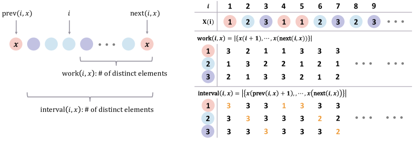
Figure 2: An example of $n=3,\mathbf{X}=(1,2,3,1,1,2,3,\cdots)$. For any $i,x$, ${\mathsf{work}}(i)$ is a permutation of $[n]$; ${\mathsf{interval}}(i,x)\geq{\mathsf{work}}(i,x)$; ${\mathsf{interval}}(i,x)$ changes only when $x(i)=x$ (highlighted in orange).

Definition 6.3 (Previous and Next Access $\mathsf{prev}(i,x)$ and $\mathsf{next}(i,x)$).

Let $\mathsf{prev}(i,x)$ be the previous access of item $x$ at or before time $i$, i.e, $\mathsf{prev}(i,x)\coloneqq\max\left\{i^{\prime}\leq i~{}\middle|~{}x(i^{\prime})=x\right\}.$ Let $\mathsf{next}(i,x)$ to be the next access of item $x$ after time $i$, i.e, $\mathsf{next}(i,x)\coloneqq\min\left\{i^{\prime}>i~{}\middle|~{}x(i^{\prime})=x\right\}.$

Definition 6.4 (Interval-Set Size ${\mathsf{interval}}(i,x)$).

Define the Interval-Set Size ${\mathsf{interval}}(i,x)$ to be the number of distinct items accessed between the previous access of item $x$ at or before time $i$ and the next access of item $x$ after time $i$. That is,

$${\mathsf{interval}}(i,x):=|\{x(\mathsf{prev}(i,x)+1),\cdots,x(\mathsf{next}(i,x))\}|.$$

If $x$ does not appear after time $i$, we define ${\mathsf{interval}}(i,x)\coloneqq n.$

Definition 6.5 (Working-Set Size ${\mathsf{work}}(i,x)$).

Define the Working-Set Size ${\mathsf{work}}(i,x)$ to be the number of distinct items accessed between time $i$ and the next access of item $x$ after time $i$. That is,

$${\mathsf{work}}(i,x)\coloneqq\left|\{x(i+1),\cdots,x(\mathsf{next}(i,x))\}\right|.$$

If $x$ does not appear after time $i$, we define ${\mathsf{work}}(i,x)\coloneqq n.$

Definition 6.6 (Interval Set Priority $\mathsf{isp}(i,x)$).

Define the time-varying priority as the reciprocal of the square of one plus interval-set size. That is,

$$\mathsf{isp}(i,x)=\frac{1}{(1+{\mathsf{interval}}(i,x))^{2}}$$

Next, we will show that the interval set priority is $O(1)$ for any time $i\in[m]$ in Lemma 6.7. The proof has three steps. Firstly, the working-set size at time $i$ is always a permutation of $[n]$. Secondly, for any $i\in[m],x\in[n]$, the interval-set size is always no less than the working-set size. Therefore, for any $i\in[m]$,the $l_{1}$ norm of interval set priority vector $\mathsf{isp}(i)=:(\mathsf{isp}(i,1),\cdots,\mathsf{isp}(i,n))$ can be upper bounded by $\sum_{j=1}^{n}1/(1+j)^{2}=O(1)$.

Lemma 6.7 (Norm Bound for Interval Set Priority).

Fix any timestamp $i\in[m]$,

$$\sum_{j=1}^{n}\mathsf{isp}(i,j)=O(1).$$

Proof.

We first show that at any time $i\in[m]$, the working-set size is a permutation of $[n]$. By definition, ${\mathsf{work}}(i,x)$ is the number of items $y$ such that $\mathsf{next}(i,y)\leq\mathsf{next}(i,x)$. Let $\pi_{1},\cdots,\pi_{n}$ be a permutation of all items $[n]$ in the order of increasing $\mathsf{next}(i,x)$. Then for any item $x$, ${\mathsf{work}}(i,x)$ is the index of $x$ in $\pi$. So the sum of the reciprocal of squared ${\mathsf{work}}(i,x)$ is upper bounded by

$$\sum_{j=1}^{n}\frac{1}{(1+{\mathsf{work}}(i,j))^{2}}=\sum_{j=1}^{n}\frac{1}{(1+j)^{2}}=\Theta(1).$$

Secondly, recall that $\mathsf{prev}(i,x)\leq i$, and hence for any $i\in[m],x\in[n]$, ${\mathsf{interval}}(i,x)\geq{\mathsf{work}}(i,x).$ So we have the upper bound for interval set priority as follows.

$$\sum_{j=1}^{n}\mathsf{isp}(i,j)=\sum_{j=1}^{n}\frac{1}{(1+{\mathsf{interval}}(i,x))^{2}}\leq\sum_{j=1}^{n}\frac{1}{(1+{\mathsf{work}}(i,j))^{2}}=O(1).$$

∎

Since we have shown the interval set priority has constant $l_{1}$ norm and in each timestamp, we only update one item’s priority. We are ready to prove and show the efficiency of the corresponding B-Treap.

Theorem 6.8 (Dynamic B-Treaps with Interval Set Priority).

With known interval set priority $\mathsf{isp}(i,x(i)),i\in[m]$ and a branching factor $B=\Omega(\ln^{1.1}n)$, there is a randomized data structure that maintains a B-Tree $T^{B}$ over $[n]$ such that when accessing the item $x(i)$ at time $i$, the expected depth of item $x(i)$ is $O(\log_{B}(1+{\mathsf{interval}}(i,x(i)))).$ The expected total cost for processing the whole access sequence $\mathbf{X}$ is

$$\mathsf{cost}(\mathbf{X},\mathsf{isp})=O\left(n\log_{B}n+\sum_{i=1}^{m}\log_{B}(1+{\mathsf{interval}}(i,x(i)))\right).$$

Furthermore, for $\delta>0$, by setting $B=O(n^{1/2-\delta})$, the guarantees hold with probability $1-\delta$.

Proof.

We apply Theorem 6.1 with $w_{i,j}=\mathsf{isp}(i,x),i\in[m],x\in[n]$. By Lemma 6.7, we know $\|w(i)\|=O(1),\mathrm{\text{ for all }}i\in[m]$. Also by definition of $\mathsf{isp}(i,x)$, for any $x\in[n]$, $\mathsf{isp}(i-1,x)\neq\mathsf{isp}(i,x)$ only when $x(i)=x$. So for each time $i$, at most one item (i.e., $x(i)$) changes its priority. So we have the total cost

$$\mathsf{cost}(\mathbf{X},\mathsf{isp}) =O\left(n\log_{B}n+2\sum_{i=1}^{m}\log_{B}(1+{\mathsf{interval}}(i,x(i)))+4\sum_{i=1}^{m}\log_{B}(1+{\mathsf{interval}}(i,x(i)))\right)$$

$$=O\left(n\log_{B}n+6\sum_{i=1}^{m}\log_{B}(1+{\mathsf{interval}}(i,x(i)))\right)$$

The last step comes from the definition of ${\mathsf{interval}}(i,x)$, which is no greater than $n$. ∎

Remark.

Consider two sequences with length $m$, $\mathbf{X}_{1}=(1,2,\cdots,n,1,2,\cdots,n,\cdots,1,2,\cdots,n)$, $\mathbf{X}_{2}=(1,1,\cdots,1,2,2,\cdots,2,\cdots,n,n,\cdots,n)$. Two sequences have the same total cost if we have a fixed score. However, $X_{2}$ should have less cost because of its repeated pattern. Given the frequency ${\mathsf{freq}}$ as a time-invariant priority, by Lemma 5.3, the optimal static costs are

$$\mathsf{cost}(\mathbf{X}_{1},{\mathsf{freq}})=\mathsf{cost}(\mathbf{X}_{2},{\mathsf{freq}})=O(m\log_{B}n).$$

But for the dynamic B-Trees, with the interval set priority, we calculate both costs from Theorem 6.8 as

$$\mathsf{cost}(\mathbf{X}_{1},\mathsf{isp})=O(m\log_{B}(n+1)),\mathsf{cost}(\mathbf{X}_{2},\mathsf{isp})=O(n\log_{B}n+m\log_{B}3).$$

This means that our proposed priority can better capture the timing pattern of the sequence and thus can even do better than the optimal static setting.

Theorem 6.9 (Dynamic B-Treaps with Predicted Interval Set Priority).

With unknown interval set priority $\mathsf{isp}(i,x(i)),i\in[m]$, there exists a machine learning oracle that gives their predictions $\widetilde{\mathsf{isp}}(i,x(i)),i\in[m]$ satisfying $|\mathsf{isp}(i,x(i))|>1/{\mathrm{poly}}(n)$ and the mean absolute error (MAE) is less than $\varepsilon>0$, i.e., $\sum_{i=1}^{m}|\mathsf{isp}(i,x(i))-\widetilde{\mathsf{isp}}(i,x(i))|\leq\varepsilon$. Let the branching factor $B=\Omega(\ln^{1/(1-\alpha)}n)$. Then there is a randomized data structure that maintains a B-Tree $T^{B}$ over $[n]$ such that when accessing the item $x(i)$ at time $i$, the expected depth of item $x(i)$ is $O(\log_{B}(1+{\mathsf{interval}}(i,x(i)))).$ The expected total cost for processing the whole access sequence $\mathbf{X}$ is

$$\mathsf{cost}(\mathbf{X},\widetilde{\mathsf{isp}})=\mathsf{cost}(X,\mathsf{isp})+O(m\log_{B}(1+n\varepsilon/m)).$$

Furthermore, for $\delta>0$, by setting $B=O(n^{1/2-\delta})$, the guarantees hold with probability $1-\delta$.

Proof.

By the definition of interval set priority, one item will change its priority at time $i$ only when it is accessed at time $i$. That is, for any $x\in[n]$, $\widetilde{\mathsf{isp}}(i-1,x)\neq\widetilde{\mathsf{isp}}(i,x)$ only when $x(i)=x$. In other words, at time $i$, we only need to learn and update $\widetilde{\mathsf{isp}}(i,x(i))$. Denote $\mathbf{isp}=(\mathsf{isp}(1,x(1),\cdots,\mathsf{isp}(m,x(m))),\widetilde{\mathbf{isp}}=(\widetilde{\mathsf{isp}}(1,x(1)),\cdots,(m,x(m)))$. So we can bound the $l_{1}$ norm of $\widetilde{\mathbf{isp}}$ as

$$\|\widetilde{\mathbf{isp}}\|_{1}\leq\|\mathbf{isp}\|_{1}+|\widetilde{\mathbf{isp}}(i,x(i))-\mathbf{isp}(i,x(i))|=O(1)$$

The last step comes from Lemma 6.7 and the bounded MAE of the prediction. Hence we can apply Theorem 6.2 with $\widetilde{w}_{i,j}=\widetilde{\mathsf{isp}}(i,x),i\in[m],x\in[n]$. Define $\varepsilon_{i,j}=\widetilde{\mathsf{isp}}(i,j)-\mathsf{isp}(i,j)$, and we get the total cost

$$\mathsf{cost}(\mathbf{X},\widetilde{\mathsf{isp}}) =O\left(n\log_{B}n+2\sum_{i=1}^{m}\log_{B}\frac{1}{w_{i,x(i)}}+2\sum_{i=1}^{m}\log_{B}\left(1+n|\varepsilon_{i,x(i)}|\right)\right)$$

$$=\mathsf{cost}(\mathbf{X},\mathsf{isp})+\sum_{i=1}^{m}\log_{B}\left(1+n|\varepsilon_{i,x(i)}|\right)$$

$$\leq\mathsf{cost}(\mathbf{X},\mathsf{isp})+O(m\log_{B}(1+n\varepsilon/m))$$

The last step is derived from Jensen’s Inequality. ∎

References

- [AL63] M AdelsonVelskii and Evgenii Mikhailovich Landis “An algorithm for the organization of information”, 1963
- [AM78] Brian Allen and J. Munro “Self-Organizing Binary Search Trees” In J. ACM 25.4, 1978, pp. 526–535
- [APT22] Yossi Azar, Debmalya Panigrahi and Noam Touitou “Online graph algorithms with predictions” In Proceedings of the 2022 Annual ACM-SIAM Symposium on Discrete Algorithms (SODA), 2022, pp. 35–66 SIAM
- [AS89] Cecilia R Aragon and Raimund Seidel “Randomized search trees” In FOCS 30, 1989, pp. 540–545
- [BCDI07] Mihai Bădoiu, Richard Cole, Erik D Demaine and John Iacono “A unified access bound on comparison-based dynamic dictionaries” In Theoretical Computer Science 382.2 Elsevier, 2007, pp. 86–96
- [BCIKL20] Prosenjit Bose, Jean Cardinal, John Iacono, Grigorios Koumoutsos and Stefan Langerman “Competitive online search trees on trees” In Proceedings of the 14th Annual ACM-SIAM Symposium on Discrete Algorithms (SODA), 2020, pp. 1878–1891 SIAM
- [BEHK16] Michael A Bender, Roozbeh Ebrahimi, Haodong Hu and Bradley C Kuszmaul “B-trees and Cache-Oblivious B-trees with Different-Sized Atomic Keys” In ACM Transactions on Database Systems (TODS) 41.3 ACM New York, NY, USA, 2016, pp. 1–33
- [BF03] Gerth Stølting Brodal and Rolf Fagerberg “Lower bounds for external memory dictionaries.” In SODA 3, 2003, pp. 546–554
- [BGVW00] Adam L Buchsbaum, Michael H Goldwasser, Suresh Venkatasubramanian and Jeffery R Westbrook “On external memory graph traversal.” In SODA, 2000, pp. 859–860
- [BR98] Guy E. Blelloch and Margaret Reid-Miller “Fast Set Operations Using Treaps” In Proceedings of the Tenth Annual ACM Symposium on Parallel Algorithms and Architectures, SPAA ’98, Puerto Vallarta, Mexico, June 28 - July 2, 1998 ACM, 1998, pp. 16–26
- [Bro14] Trevor Brown “B-slack trees: Space Efficient B-trees” In Scandinavian Workshop on Algorithm Theory, 2014, pp. 122–133 Springer
- [Bro17] Trevor Brown “B-slack trees: Highly Space Efficient B-trees” In arXiv preprint arXiv:1712.05020, 2017
- [Can20] Clément L Canonne “A short note on learning discrete distributions” In arXiv preprint arXiv:2002.11457, 2020
- [CCS19] Parinya Chalermsook, Julia Chuzhoy and Thatchaphol Saranurak “Pinning down the strong Wilber 1 bound for binary search trees” In arXiv preprint arXiv:1912.02900, 2019
- [CEILNRSWWZ22] Justin Y Chen, Talya Eden, Piotr Indyk, Honghao Lin, Shyam Narayanan, Ronitt Rubinfeld, Sandeep Silwal, Tal Wagner, David P Woodruff and Michael Zhang “Triangle and Four Cycle Counting with Predictions in Graph Streams” In arXiv preprint arXiv:2203.09572, 2022
- [CI21] Justin Y Chen and Piotr Indyk “Online Bipartite Matching with Predicted Degrees” In arXiv preprint arXiv:2110.11439, 2021
- [CLRS09] Thomas H. Cormen, Charles E. Leiserson, Ronald L. Rivest and Clifford Stein “Introduction to Algorithms, 3rd Edition” MIT Press, 2009 URL: http://mitpress.mit.edu/books/introduction-algorithms
- [CM05] Graham Cormode and Shan Muthukrishnan “An improved data stream summary: the count-min sketch and its applications” In Journal of Algorithms 55.1 Elsevier, 2005, pp. 58–75
- [CMSS00] Richard Cole, Bud Mishra, Jeanette Schmidt and Alan Siegel “On the dynamic finger conjecture for splay trees. Part I: Splay sorting log n-block sequences” In SIAM Journal on Computing 30.1 SIAM, 2000, pp. 1–43
- [Col00] Richard Cole “On the dynamic finger conjecture for splay trees. Part II: The proof” In SIAM Journal on Computing 30.1 SIAM, 2000, pp. 44–85
- [CSVZ22] Justin Chen, Sandeep Silwal, Ali Vakilian and Fred Zhang “Faster fundamental graph algorithms via learned predictions” In International Conference on Machine Learning, 2022, pp. 3583–3602 PMLR
- [DHIKP09] Erik D Demaine, Dion Harmon, John Iacono, Daniel Kane and Mihai Patraşcu “The geometry of binary search trees” In Proceedings of the 20th annual ACM-SIAM symposium on Discrete algorithms (SODA), 2009, pp. 496–505 SIAM
- [DHIP07] Erik D Demaine, Dion Harmon, John Iacono and Mihai Patraşcu “Dynamic optimality—almost” In SIAM Journal on Computing 37.1 SIAM, 2007, pp. 240–251
- [DILMV21] Michael Dinitz, Sungjin Im, Thomas Lavastida, Benjamin Moseley and Sergei Vassilvitskii “Faster matchings via learned duals” In Advances in Neural Information Processing Systems 34, 2021, pp. 10393–10406
- [DMYWDLZCGK+20] Jialin Ding, Umar Farooq Minhas, Jia Yu, Chi Wang, Jaeyoung Do, Yinan Li, Hantian Zhang, Badrish Chandramouli, Johannes Gehrke and Donald Kossmann “ALEX: an updatable adaptive learned index” In Proceedings of the 2020 ACM SIGMOD International Conference on Management of Data, 2020, pp. 969–984
- [DS09] Jonathan C Derryberry and Daniel D Sleator “Skip-splay: Toward achieving the unified bound in the BST model” In Workshop on Algorithms and Data Structures, 2009, pp. 194–205 Springer
- [EFSWZ21] Jon Ergun, Zhili Feng, Sandeep Silwal, David P Woodruff and Samson Zhou “Learning-Augmented -means Clustering” In arXiv preprint arXiv:2110.14094, 2021
- [ELMS22] Thomas Erlebach, Murilo Santos Lima, Nicole Megow and Jens Schlöter “Learning-Augmented Query Policies for Minimum Spanning Tree with Uncertainty” In arXiv preprint arXiv:2206.15201, 2022
- [FHM19] Rolf Fagerberg, David Hammer and Ulrich Meyer “On Optimal Balance in B-Trees: What Does It Cost to Stay in Perfect Shape?” In 30th International Symposium on Algorithms and Computation (ISAAC 2019), 2019 Schloss Dagstuhl-Leibniz-Zentrum fuer Informatik
- [FLV20] Paolo Ferragina, Fabrizio Lillo and Giorgio Vinciguerra “Why are learned indexes so effective?” In International Conference on Machine Learning, 2020, pp. 3123–3132 PMLR
- [FV20] Paolo Ferragina and Giorgio Vinciguerra “The PGM-index: a fully-dynamic compressed learned index with provable worst-case bounds” In Proceedings of the VLDB Endowment 13.8 VLDB Endowment, 2020, pp. 1162–1175
- [Gol08] Daniel Golovin “Uniquely represented data structures with applications to privacy”, 2008
- [Gol09] Daniel Golovin “B-treaps: A uniquely represented alternative to B-trees” In Automata, Languages and Programming: 36th International Colloquium, ICALP 2009, Rhodes, Greece, July 5-12, 2009, Proceedings, Part I 36, 2009, pp. 487–499 Springer
- [GS78] Leo J Guibas and Robert Sedgewick “A dichromatic framework for balanced trees” In 19th Annual Symposium on Foundations of Computer Science (sfcs 1978), 1978, pp. 8–21 IEEE
- [HIKV19] Chen-Yu Hsu, Piotr Indyk, Dina Katabi and Ali Vakilian “Learning-Based Frequency Estimation Algorithms.” In International Conference on Learning Representations, 2019
- [HT70] TC Hu and AC Tucker “Optimum Binary Search Trees.”, 1970
- [Iac01] John Iacono “Alternatives to splay trees with worst-case access times” In Proceedings of the twelfth annual ACM-SIAM symposium on Discrete algorithms, 2001, pp. 516–522
- [Iac05] John Iacono “Key-independent optimality” In Algorithmica 42.1 Springer, 2005, pp. 3–10
- [Iac13] John Iacono “In pursuit of the dynamic optimality conjecture” In Space-Efficient Data Structures, Streams, and Algorithms Springer, 2013, pp. 236–250
- [JDO99] Chris Jermaine, Anindya Datta and Edward Omiecinski “A novel index supporting high volume data warehouse insertion” In VLDB 99, 1999, pp. 235–246
- [JLLRW20] Tanqiu Jiang, Yi Li, Honghao Lin, Yisong Ruan and David P Woodruff “Learning-augmented data stream algorithms” In ICLR, 2020
- [JNSSK97] HV Jagadish, PPS Narayan, Sridhar Seshadri, S Sudarshan and Rama Kanneganti “Incremental organization for data recording and warehousing” In VLDB, 1997, pp. 16–25
- [KBCDP18] Tim Kraska, Alex Beutel, Ed H Chi, Jeffrey Dean and Neoklis Polyzotis “The case for learned index structures” In Proceedings of the 2018 international conference on management of data, 2018, pp. 489–504
- [KLR96] Marek Karpinski, Lawrence L Larmore and Wojciech Rytter “Sequential and Parallel Subquadratic Work Algorithms for Constructing Approximately Optimal Binary Search Trees.” In SODA, 1996, pp. 36–41 Citeseer
- [LLW22] Honghao Lin, Tian Luo and David Woodruff “Learning Augmented Binary Search Trees” In International Conference on Machine Learning, 2022, pp. 13431–13440 PMLR
- [LMRX20] Thomas Lavastida, Benjamin Moseley, R Ravi and Chenyang Xu “Learnable and instance-robust predictions for online matching, flows and load balancing” In arXiv preprint arXiv:2011.11743, 2020
- [MA13] Giorgos Margaritis and Stergios V Anastasiadis “Efficient range-based storage management for scalable datastores” In IEEE Transactions on Parallel and Distributed Systems 25.11 IEEE, 2013, pp. 2851–2866
- [Meh75] Kurt Mehlhorn “Best possible bounds for the weighted path length of optimum binary search trees” In Automata Theory and Formal Languages, 2nd GI Conference, Kaiserslautern, May 20-23, 1975 33, Lecture Notes in Computer Science Springer, 1975, pp. 31–41
- [Meh75a] Kurt Mehlhorn “Nearly optimal binary search trees” In Acta Informatica 5.4 Springer, 1975, pp. 287–295
- [MV20] Michael Mitzenmacher and Sergei Vassilvitskii “Algorithms with predictions” In arXiv preprint arXiv:2006.09123, 2020
- [OCGO96] Patrick O’Neil, Edward Cheng, Dieter Gawlick and Elizabeth O’Neil “The log-structured merge-tree (LSM-tree)” In Acta Informatica 33 Springer, 1996, pp. 351–385
- [PZ22] Adam Polak and Maksym Zub “Learning-Augmented Maximum Flow” In arXiv preprint arXiv:2207.12911, 2022
- [RS81] Arnold L Rosenberg and Lawrence Snyder “Time-and space-optimality in B-trees” In ACM Transactions on Database Systems (TODS) 6.1 ACM New York, NY, USA, 1981, pp. 174–193
- [SS23] Roodabeh Safavi and Martin P Seybold “B-Treaps Revised: Write Efficient Randomized Block Search Trees with High Load” In arXiv preprint arXiv:2303.04722, 2023
- [ST85] Daniel Dominic Sleator and Robert Endre Tarjan “Self-Adjusting Binary Search Trees” In J. ACM 32.3, 1985, pp. 652–686
- [ST85a] Daniel Dominic Sleator and Robert Endre Tarjan “Self-adjusting binary search trees” In Journal of the ACM (JACM) 32.3 ACM New York, NY, USA, 1985, pp. 652–686
- [Vit01] Jeffrey Scott Vitter “External memory algorithms and data structures: Dealing with massive data” In ACM Computing surveys (CsUR) 33.2 ACM New York, NY, USA, 2001, pp. 209–271
- [WZCWCX21] Jiacheng Wu, Yong Zhang, Shimin Chen, Jin Wang, Yu Chen and Chunxiao Xing “Updatable learned index with precise positions” In Proceedings of the VLDB Endowment 14.8 VLDB Endowment, 2021, pp. 1276–1288
- [Yao82] F Frances Yao “Speed-up in dynamic programming” In SIAM Journal on Algebraic Discrete Methods 3.4 SIAM, 1982, pp. 532–540
- [Yi12] Ke Yi “Dynamic Indexability and the Optimality of B-trees” In Journal of the ACM (JACM) 59.4 ACM New York, NY, USA, 2012, pp. 1–19
- [ZB22] Eva Zangerle and Christine Bauer “Evaluating Recommender Systems: Survey and Framework” New York, NY, USA: Association for Computing Machinery, 2022