The aerodynamic response of a pre-stressed elastically nonlinear aileron

Abstract

We study the aerodynamic response of a pre-stressed curved aileron. Whilst the fluid flow is standard (high Reynolds air flow undisturbed at infinity), the structure is designed to have a peculiar nonlinear behavior. Specifically, the aileron has only one stable equilibrium when the external forces are vanishing, but it is bistable when relevant aerodynamic loads are applied. Hence, for sufficiently high fluid velocities, another equilibrium branch is possible. We test a prototype of such an aileron in a wind tunnel; a sudden change (snap) of the shell configuration is observed when the fluid velocity exceeds a critical threshold: the snapped configuration is characterized by sensibly lower drag. However, when the velocity is reduced to zero, the structure recovers its initial shape. A similar nonlinear behavior can have important applications for drag reduction strategies.

1 Introduction

A promising research paradigm in the recent years has been the use of smart (or responsive) materials and structures, as enhancements of the functions of machines, or, in some cases, in order to replicate some of these functions altogether [1]. Fields where this paradigm has found many applications have been, among others, robotics [2] and aeronautics [3, 4, 5]. The functions that these materials allow can be divided in two broad categories [6]: energy-related, concerning applications such as energy harvesting, or motion-related. One particular advantage is that these functions can usually be performed with reduced complexity of the final system, in that there’s less need of actuating machinery, or complex control systems (if passive actuation is used). These applications can be obtained by taking advantage of the characteristics of the materials, such as memory shape alloys [7], hydrogels, elastomers, or polymers. An alternative is that of exploiting mechanical processes, such as occurrence of instabilities. A great example of this is buckling [6], an elastic instability that gives place to high deformations and sudden energy release, and can be exploited for both energy harvesting applications, motility, or design for actuators, among others. In order to induce such mechanical processes, an interesting approach is that of taking advantage of both the characteristics of the material and of the geometry of the structure. For example, thin shells, after an incompatible elastic strain (as obtained, for example, by inelastic deformation during the production process), can result in spontaneous curvature and multi-stable behavior, which can be actuated in order to obtain complex motions or yet again for energy harvesting applications. In this work, we consider the case of a morphing shell with application in the context of aerodynamics. These shells are such that they have a pseudo-conical natural configuration, and, when clamped on one of the sides, tend to assume a curved shape, with possible bi-stable behavior when the initial curvature is chosen accordingly. The use of bistable structures has been considered already in aeronautics [8, 9], for example, for alleviation of excessive aerodynamic loads [10]. In this regard, we note some of the advantages of our approach, and of the particular features of the structure presented: the goal is to exploit the aerodynamic drag as actuation, inducing the bistable behavior after a critical loading threshold, obtaining sudden shape changes with consequent drag reduction. The system can be tuned to any critical load, and to the desired multi-stable behavior by simply changing the starting geometry before clamping, and thus is very versatile compared to other usual applications, when the material and geometry both have to be fine tuned for each particular application. Furthermore, since actuation is due to the aerodynamic load alone, there’s no need for complex actuations, such as heating, fluid supply, or chemical reactions. The dependence of the behavior on the load also means that the snap-through of the structure is trivially reversible: when the load decreases (that is, deceleration of the external flow) under a certain threshold, the structure snaps back to original configuration. This makes the shell an excellent example of smart structure in the context of aeroelasticity. It should be emphasized is that the structure is not bistable if a load is not applied: it will be shown that applying a load at the tip, after the shell is clamped at one of the sides, and increasing the force progressively, such a morphing shell can deform and snap-through, due to the emergence of a second stable configuration after a certain load threshold. This capability with a simple loading is easy to demonstrate. The purpose of this work is to demonstrate the feasibility of this approach in a more complex application, that is when the structure is under a realistic aerodynamic load. Such a load can be generated, for example, when the shell is mounted on a vehicle that moves at increasing speed: the pressure drag generated acts as an actuating force and could induce, in suitable conditions, snap-through. It remains to prove that with this complex and time dependent load, the desired behavior is still achieved. In order to do this, we study the problem both experimentally and numerically. The first part of the study is experimental: a prototype of this shell, fabricated with lamina of composite material, was studied in the wind tunnel, subject to increasing aerodynamic loads generated by an external flow. The numerical study is a simulation of the aeroelastic problem with a quasi-static approach: we simulate the drag due to an external flow, solving the set of $3D$ Navier-Stokes equations, accelerating from idle to a velocity that causes snap-through, and determine the response of the structure in incremental steps, as will be clarified below. In this way, we fully explore the application of a promising smart structure in the aeroelastic context. Such a behavior can have many interesting uses, such as the case, already mentioned, of load alleviation over a certain drag threshold, complex shape changes, as well as energy harvesting. Moreover, the results will confirm the feasibility of using reduced models for the description of the (non-linear) structural response to aerodynamic loads. In section 2, the problem is stated in more detail. In section 3 we report the features of the structure, and the setup and results of the experimental study. In section 4 we describe the numerical study and we report numerical results, and their comparison with the experimental ones. We draw conclusions and perspectives on possible future work in section 5.

2 Problem statement

The structure studied is a pre-stressed shell made of composite laminate shown in Fig. 1 (more details on the material are given in section 3.1). In its natural stress-free configuration, the shell has rectangular planform with sides $L_{x}$ and $L_{y}$; one side of the shell has curvature $h_{1}$, while the other is flat. We refer the interested reader to [11, 12] where a similar class of shells subject to clamped boundary conditions was extensively studied. When, the curved side is clamped, the shell equilibrium shape is changed into the curved profile shown in figure 1B. This equilibrium shape is associated with a relevant stress field which is the principal responsible of the nonlinear elastic behavior of such a structure.

In the case studied, the natural configuration (namely $h_{1}$) is chosen such that the shell is monostable after clamping, but can become bistable after application of external loads. As anticipated, this is the novelty of our approach, since bistability is not induced by means of complex phenomena or actuations, but is rather obtained, in a reversible manner, only as a result of external forces, in certain loading conditions.

Hence, when the applied external forces are vanishing, the curved equilibrium shape shown in Fig. 1B is the only stable equilibrium. However, the presence of forces could alter the shell stability behavior. For instance, we report in Fig. 2 the shell behavior under the application of a dead load $F$ at its tip.

As such a force is progressively increased we compute all the possible stable equilibria of the shell and, in particular, their tip displacements shown in the horizontal axis of Fig. 2. To this aim, we find all the minima of a reduced form of the elastic elastic energy of the shell as obtained in [13]; deatils of this derivation are reported in A. The energy has a polynomial expression and for a simple follower load, the system to be solved is simple enough that global minima can be found, with standard numerical tools, for each value of applied force. In figure 2, it can be seen that tho different solution branches are present: starting from the initial clamped configuration, for a force of value $F<F_{2}$, the behavior is hyperelastic. If the load is decreased, the solution would follow the same branch in the opposite direction. However, after a certain loading threshold $F_{1}$ the structure becomes bistable, and if the load is high enough, $F>F_{2}$, only the branch that emerges for higher force values remains. The structure will snap to the new branch, which is also stable and therefore can be followed by increasing or decreasing the load, again with an hyperelastic behavior. Only when the force decreases under the bistability threshold value, $F<F_{1}$, does the structure snap back to the first branch, which is the only one stable for low values of $F$. It can be readily noted that the two thresholds are different, $F_{1}<F_{2}$. Therefore, the structure exhibits an hysteresis in the loop obtained by loading and then releasing at the tip, if a certain threshold is exceeded. Again, it should be emphasized that this behavior was obtained through forcing alone, and no other means of actuation were necessary.

We investigate the behavior of such a structure when it is invested by a fluid flow in the axial direction with undisturbed velocity $\big{(}U_{\infty}$.

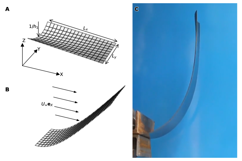
Figure 1: (A) natural configuration of the shell. (B) equilibrium shape of the shell after clamping at the initially curved side. Incoming flow velocity $\bm{u}_{\infty}$ aligned with the $X$ direction, is represented. (C) snapshot of the prototype used for the experiments, attaining a curved shape after clamping.

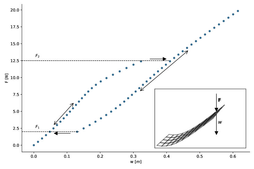
Figure 2: Displacement of the tip of the shell, in the clamped configuration, as function of the value of a follower load, applied at the tip as well. Possible movements along the solution branches, and thresholds at which jumps between the two can be attained, are depicted.

This experiment serves as a motivation for the rest of the work: the follower force at the tip is will be substituted with an aerodynamic load, as shown already in figure 1. The action of the flow will be that of forcing the structure to open into a more streamlined shape. The flow velocity $U_{\infty}$ is supposed to increase in a quasi-static fashion, up to a threshold when multistable behavior occurs, and is subsequently decreased back to zero. This loop is the actuation that we want to investigate. The fluid of the external flow is supposed to be air, since we study the shell with the goal of showing its suitability for applications in the automotive or aerospace field, where the induced bistability could be exploited, e.g., for drag reduction.

3 Experimental evidence

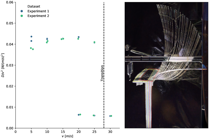
Figure 3: Left: experimental results in terms of measured drag forces, as function of the external flow velocity. Right: superposition of snapshots of an experimental run in wind tunnel, during an acceleration of the external flow until the shell snaps to the other stable configuration.

3.1 Materials and methods

The constitutive material of the shell studied in this work is a composite laminate, realized with the stacking of 8 layers, each an unidirectional carbon ply TenCate TC275-1 Epoxy Resin System, cured at $135^{\circ}C$ (see [12] for a more detailed description of this composite shell). The stacking sequence of the layers, for a chosen $\alpha=45^{\circ}$, is antisymmetric:

$$[-\alpha/+\alpha/+\alpha/-\alpha/+\alpha/-\alpha/-\alpha/+\alpha],$$ (1)

The stiffness matrices of the composite laminate, needed for the derivation of the elastic model (see equation (7)) are:

$$\frac{\bm{A}}{A_{11}}=\frac{\bm{D}}{D_{11}}=\begin{pmatrix}1&\nu&0\\ \nu&\beta&0\\ 0&0&\gamma\end{pmatrix},\qquad\bm{B}=\bm{0}.$$ (2)

For the material use it holds $\beta=1.0$, $\nu=0.851$, $\gamma=0.858$, $A_{11}=4.59\cdot 10^{7}\frac{N}{m}$ and $D_{11}=3.82Nm$. The starting curvatures are $h_{1}=\frac{1}{r_{1}}$ and $h_{2}=\frac{1}{r_{2}}$, with $r_{1}=0.064m$ and $r_{2}=\infty$, meaning that only the side to be clamped is curved, while the other is flat. The final thickness of the laminate is $1mm$ ($0.125mm$ for each layer), while the dimensions of the natural configuration are $L_{x}=0.33m$ and $L_{y}=0.15m$ (see figure 1).

3.1.1 Experimental setup

An experimental campaign was run in the wind tunnel facility at the Fluid Mechanics Lab at Sapienza University of Rome. The wing was supported in such a way that the structure is the only obstacle in an otherwise undisturbed flow. A view of the support of the shell is given in figure 3 right: the side to be clamped is closed between two plates, and four screws are inserted and tightened to pull the plates together. The screws are positioned laterally with respect to the shell, that is, no holes are made on the structure. Two small layers of Styrofoam protect the shell avoiding direct contact with the plates. This clamping therefore is not perfect, in that the shell has a small, non-zero curvature within the two plates. This can be observed also from the fact that the two clamping plates are slightly curved: in correspondence of the screws, they are closed together, while some distance arises in-between due to the presence of the plate. Between each experimental run, this distance is measured in order to assure at least that it is always the same value. A perfect clamping would cause the risk of permanently deform the shell, preventing he reproduction of the experiment. The support of the wing was connected to a load cell in order to measure the drag force. During each experimental run, the velocity of the flow was varied in a controlled manner in small increments, from $0$ up to around $30m/s$. The increase was stopped after snap-through was observed, and was slow enough in order to have a loading as close as possible to quasi-static. Once the maximum velocity was reached, a slow deceleration was imposed to get back to the starting velocity value. Several measurements of this acceleration-deceleration loop have been performed, paying particular attention to the threshold velocity values and to the reproducibility of the acceleration-deceleration loop response of the structure. At high velocities, close to the snap-through threshold, the support showed some degree of deformation. This can be observed in figure 3 right: before the snap transition, the support has rotated slightly in direction of the flow. Once the shell snaps to the other stable configuration, the rotation vanishes. From the series of snapshots of the experiments, the maximum rotation angle is estimated to be around $3$ degrees.

3.2 Results

In the experiments, velocity was gradually increased from rest until a snap-through was observed, then slowly decreased back to the starting value. In figure 3, we report the experimental measurements of drag on the shell during this loop. Several measurements were performed in order to highlight the reproducibility of the phenomena. From the experimental drag results, it is clear that a snap-through occurs for a value of incoming flow velocity of about $29m/s$. When this happens, the drag value measured on the structure falls, since the new stable equilibria is an almost flat configuration. This new configuration is maintained even when velocity is then decreased, gradually stopping the flow of the wind tunnel. This implies that the equilibrium state is moving along a stable branch different from the initial one. Only when velocity is considerably lower, around $15-17m/s$, does the structure snap-back to the original stable branch. This transition is spontaneous and requires no external intervention. This proves that the structure bi-stability can be triggered by a force of the kind generated by aerodynamic drag. At both transitions between stable branches, significant oscillations are observed: this is indicative that the stiffness of the structure is decreasing to very low values, and is typical of a snap-through scenario; when the structure snaps from one stable configuration to the other, it can be thought to have zero-stiffness. The oscillations are not shown in figure 3 because measurements during this phase are difficult to perform accurately. From figure 3 it can also be noted that the transition loop can be reproduced very accurately in different measurements.

4 Numerical evidence

With the goal of developing a numerical model capable of reproducing the experimental behavior, two different systems will be coupled: a reduced nonlinear elastic model for the shell, and a set of $3D$ Navier-Stokes equations. The fluid-structure coupling is approximated as quasi-static: indeed in the experiment the flow velocity varies slowly, and so does the structural deformation with the exception of the snap-through. Therefore, we don’t solve for the dynamic strong coupling that would result from the full the aeroelastic problem, as detailed below. The reduced shell model, derived in A, yields an elastic energy functional that is polynomial in three lagrangian coordinates

$$\mathcal{E}_{el}=\hat{\epsilon}\left(\bm{d}(q_{1},q_{3},q_{4})\right),$$ (3)

where $\bm{d}$ is the displacement field with respect to the initial (after clamping) configuration. The three coordinates (see A for their definition) have an immediate interpretation: $q_{1}$ is the curvature of the shell centerline at the point of clamping $x=0$, $q_{3}$ is the variation of curvature along the centerline, and $q_{4}$ is the curvature in the direction perpendicular to the centerline. To obtain the total energy, one has to subtract the work of the external forces, defined as:

$$F_{j}=\int_{S_{0}}\bm{F}_{v}\cdot\frac{\partial\bm{d}}{\partial q_{j}}\text{d}S_{0},\qquad j=1,3,4$$ (4)

where $\bm{F}_{v}$ is the vector field of the external forces acting on the surface of the shell. When solving the problem for a simple (or absent) forcing, such as the example in section 2 (figure 2 in particular), the system of equations is simple enough that one can find all minima by using standard routines for root finding of polynomial systems. In particular, we use Mathematica [14] and its NSolve routine. The gradient of the total energy will indeed be polynomial, and the problem reduces to finding its roots. From these solutions then the minima of the potential energy are identified, since the hessian can be calculated directly as well. This procedure yields the global stability landscape, and allows to solve for all solution branches at the same time. On the other hand, when the forcing is given by the interaction with a fluid, the force field is more complex, since now $\bm{F}_{v}=-p\bm{n}$, with $p$ pressure of the fluid, given by the solution of the external flow equations, and $\bm{n}$ the normal to the shell surface. In this case one cannot hope to solve the problem with the direct method above. We resort to finding local minima iteratively. Starting from a known solution value $q_{j}^{n}$, $j=1,3,4$, and knowing the fluid force $\bm{F}_{v}=-p^{n+1}\bm{n}$, the problem to solve is:

$$q_{j}^{n+1} =\min_{q_{j}}\mathcal{E}(q_{j},q_{j}^{n}),\qquad j=1,3,4$$ (5)

$$\mathcal{E}(q_{j},q_{j}^{n}) =\hat{\epsilon}\left(\bm{d}(q_{1},q_{3},q_{4})\right)-\Sigma_{j}F_{j}(q_{j}^{n})\cdot(q_{j}-q_{j}^{n}).$$

Several approximations have been done: in order to obtain an expression of the work in closed form, the force is supposed to be constant over the step, and is calculated for the shell configuration (on which the lagrangian forces depend implicitly) at the known initial solution $q_{j}^{n}$. This is the simplest approximation and is expected to work if the steps are small enough. Our quasi-static solution cycle is thus composed by the following sub-steps:

• start from the previous known solution, for a given state $U_{\infty}^{n}$, $p^{n}$ of the fluid and $q_{j}^{n}$ for the solid. If at beginning of simulation, $U_{\infty}^{0}=0=p^{0}$, find minimum for zero forcing to obtain starting $q_{j}^{0}$

• generate geometry of the shell given lagrangian coordinates $q_{j}^{n}$ (see A), or the starting ones $q_{j}^{0}$

• given value of external velocity $U_{\infty}^{n+1}$ at the new step, solve the external flow problem (detailed below) and calculate the new pressure field $p^{n+1}$

• calculate lagrangian forces from equation (4) and solve problem (5) to calculate the new values $q_{j}^{n+1}$

• find new local solution of the system (15) in terms of the values of $q_{1}$, $q_{3}$, $q_{4}$, using as starting point for root search the previous known solution

• move to next step

The value of external flow velocity $U_{\infty}$ ranges in a loop, in small increments, from a zero starting value to a maximum value, taken from the experiments, and then back to the starting one. This allows us to simulate a loop of acceleration and subsequent deceleration of the flow, which is the working condition in which the structure is to be studied. To perform the local minimization step, we use the scipy library.

4.1 Navier-Stokes flow simulations

The external flow problem is modelled by the steady Navier-Stokes equations. To solve these at each step, we use the OpenFOAM library. The mesh of the fluid domain is generated with the utility $snappyHexMesh$. The domain consists of a rectangular space both in the $xy$ and $xz$ planes, with a hole at the center, which coincides with the boundary of the structure in the configuration being currently studied. The center of the clamped side of the shell is positioned at the origin. The positioning of the solid surface, far from any other boundary, is consistent with the experimental set-up. The domain is large enough that the condition of undisturbed flow is attained far from the boundary of the shell. Keeping consistent with the coordinates in section 2, the surface centerline develops in the plane $xz$, and has a weak curvature in the $xy$ plane. The incoming flow is oriented in the $x$ direction, therefore hitting the surface as a bluff body when this is curled after clamping, and would be tangent to it if the shell were completely opened into a flat shape, similar to what is observed in the experiments after the structure snaps to another stable solution branch. This geometry is defined by means of an STL surface, which is generated with a python utility starting from a point sampling of the mid-surface, given from eq. (19). The solver utilized is simpleFoam, suitable for computation of a stationary solution of the Navier-Stokes equations. In figure 2, the structure has a bistable behavior when applying a force at the tip, of magnitude of the order $10\div 20N$. To estimate roughly the magnitude of the incoming flow velocity, one can calculate which velocity would produce a comparable drag force over a flat plate with the same dimensions of the structure. This results in an estimate of Reynolds number of the order of $10^{5}\div 10^{6}$, meaning that the flow is expected to be fully turbulent. At Reynolds numbers this high, we can assume that friction forces be negligible with respect to the pressure contribution. This justifies defining the fluid force field as $\bm{F}_{v}=-p\bm{n}$ in equation 4. The $k-\varepsilon$ RANS turbulence model is used for modeling of turbulence. The boundary conditions are of imposed velocity at the inlet and on the solid surface (no-slip in the latter case), while the zeroGradient, that is, Neumann boundary condition is assigned at the outlet. At the top and bottom surfaces (w.r.t. the $z$ direction) a slip condition is assigned. The two remaining surfaces are set as symmetry planes. As to the pressure, a fixed value of $0$ is set at the outlet. Turbulent wall functions corresponding to the turbulence model in use are set at the solid boundary, in order to model the boundary layer. The turbulence variables $k$ and $\varepsilon$ to be assigned at inlet are estimated with the following formula:

$$k_{\infty} =\frac{3}{2}(IU_{\infty})^{2},$$ (6)

$$\varepsilon_{\infty} =\frac{1}{L_{y}}(\frac{2}{3}k_{\infty})^{\frac{3}{2}},$$

where $U_{\infty}$ is the velocity far from the structure, assigned at the inlet, and in our case $I=0.1$ and $L_{y}$, introduced in section 2, is taken as reference length. Discretization of the Navier-Stokes equations is done with finite volumes, with second order accuracy for regular meshes. The discretization of the fluxes of all variables is done with an interpolation scheme that ensures stability (TVD), and we employ schemes in their bounded variant, that is, schemes with an additional term that penalizes the continuity (incompressibility) errors. This term, added to the discretized equations, is consistent in that it vanishes when convergence to a solution is reached.

4.2 Numerical results

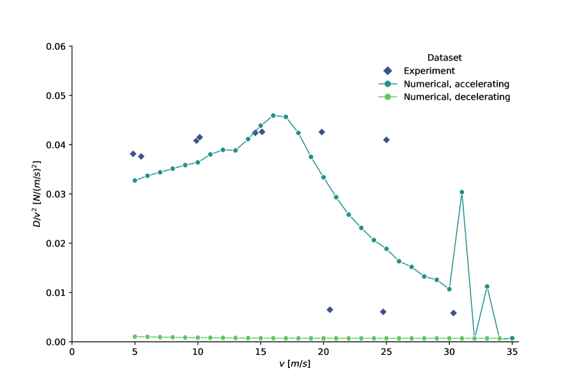
Figure 4: Comparison between numerical and experimental results in terms of measured drag forces, as function of the external flow velocity.

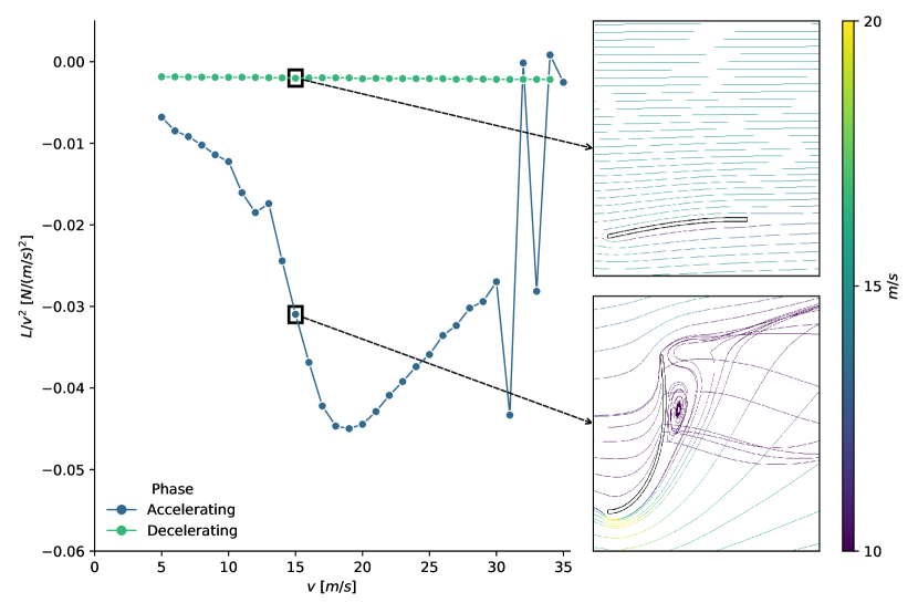
Figure 5: Numerical results, given as function of outer flow velocity. Left: lift force (force in $z$ direction). Right: snapshots of streamlines, from numerical simulations.

The results of the numerical model introduced in this section are compared with the experimental benchmark. In figure 4, the drag force values resulting from an acceleration-deceleration loop of are reported, together with the experimental results. In figure 5 instead, the numerical results for the lift force are given, for which there is no experimental data (for our choice of coordinates, as in figure 1, lift and drag are the force components $z$ and $x$, respectively). The solution procedure allows us to identify two branches of solutions. The first one originates from the equilibrium solution for zero external forcing. When velocity is increased past a certain threshold, which can be individuated around $29-30m/s$, the system shows strong oscillations and stabilizes on a second branch, which is stable and corresponds to much lower values of drag. This second branch can then be followed increasing or decreasing the flow velocity, meaning that after the jump, the shell has an hyperelastic behavior on a different stable branch with respect to the starting one, as was seen in the example of figure 2. The branch remains stable even if velocity is decreased, gradually, back to the starting value. The second transition, from the second branch back to the starting one, is not observed numerically. The initial numerical branch, that is, the solution branch obtained following starting from the equilibrium state for zero forcing, agrees qualitatively with the experimental results of the acceleration phase. Differences in the observed values of the drag, and in the reproduced behavior can be attributed to several factors: the transient contributions are neglected in the numerics, and the acceleration/deceleration of the flow in the experiments, even though the velocity variations were gradual, could be a factor in correspondence of the snap transitions between stable branches. Another factor, as reported in section 3, is that in the experiments, the support over which the shell was fixed showed some degree of rotation at the higher velocities, as is highlighted in figure 3 right. Furthermore, it should be noted that inaccuracies can also be attributed to the uncertainty in the measurement of the thickness of the shell: the bending stiffness scales with $t^{3}$, that is, with the third power of the thickness, thus small variations can result in non negligible stiffness changes.

5 Conclusions

Our contribution is two-fold: we presented an application of smart structure, where multi-stability is harnessed to induce interesting behavior. The shell considered here can be bistable when under external aerodynamic loading, proving valuable for drag reduction strategies. In particular, this bistable behavior, which is triggered by forces, is reversible and therefore no actuation is necessary. This behavior was first observed with a simple experiment applying a point follower load. With an experimental campaign in a wind tunnel, we then confirmed that an aerodynamic force can trigger the same bistable, and reversible, behavior. Moreover, we presented a numerical study of the aeroelastic problem, and proposed a strategy based on a reduced nonlinear elastic model and $3D$ steady Navier-Stokes fluid model. This approach has the advantage of being computationally inexpensive with respect to a fully coupled aeroelastic FSI simulation. The model is capable of predicting the existence of different solution branches, and reproduces the experimental data, for the accelerating flow phase, with an acceptable accuracy. The snap transition between stable branches at high flow velocities is predicted by the numerical model, while the snap back is not reproduced. We discussed the factors that have to be improved to improve the behavior reproduction of the numerical model. In particular, the effective clamping conditions in the experiments need to be assessed with care, as well as the possible deformations of the support for high aerodynamic loads. A further development could be assessing the performance of a more complicated solid model: the shallow shell model works well when the curvatures are low, which was not a limitation in our case since, due to our setup, the aeroelastic load forces the shell to assume a progressively more streamlined (and flat) shape. The solid model depends, through the ansatz of the displacement field (9), on five lagrangian coordinates. The model could be enriched, adding polynomial terms to the ansatz, which could result in more accurate predictions.

Appendix A Shell model

A.1 Derivation of the nonlinear reduced model

We refer to the design of multi-stable shells in [11], for which a model is given within the assumptions of the shallow shell approximation, starting from the Foppl von-Kármán theory. In this approximation, the following constitutive relations hold

$$\bm{t} =\bm{A}(\bm{e}-\bm{f})+\bm{B}(\bm{k}-\bm{h}),$$ (7)

$$\bm{m} =\bm{D}(\bm{k}-\bm{h})+\bm{B}^{T}(\bm{e}-\bm{f}),$$

where, in vector notation, the membrane stresses $\bm{t}$, the bending moments $\bm{m}$, the membrane strains $\bm{e}$ and the curvatures $\bm{k}$ appear, with $\bm{f}$ and $\bm{h}$ stresses and curvatures of the natural configuration. $\bm{A}$ and $\bm{D}$ are the stiffness matrices, given in section 3.1. The particular choice of starting natural configuration is what will induce the multi-stable behavior; no inelastic pre-stresses are applied, and therefore $\bm{f}=\bm{0}$, $\bm{h}\neq\bm{0}$. The shell has a natural configuration which is pseudo-conic. Thus, the mathematical expression of its mid-surface will be of the form:

$$S_{0} =\{(x,y,w_{0}(x,y)),0\leq x\leq L_{x},-L_{y}/2\leq y\leq L_{y}/2\},$$ (8)

$$w_{0}(x,y) =\frac{y^{2}}{2}\left(h_{1}+(h_{2}-h_{1})\frac{x}{L_{x}}\right),$$

where $w$ is the displacement in the $z$ direction, and the shell in its flat configuration lies in the $xy$ plane. $h_{1}$ and $h_{2}$ determine the curvatures of the natural configuration. In the working configuration, the shell will be clamped at the side $x=0$, which is the side of curvature $h_{1}$.

A.1.1 Reduced nonlinear model

A model for the response of the shell under aerodynamic loads is needed: a low-dimensional model [13] was proven to be effective in describing the the deformation of the shell under loading, as well as predicting eventual bifurcations and the post-critical behavior. More in detail, an ansatz is given for the expression of the transverse displacement field:

$$w(x,y)=q_{1}\frac{x^{2}}{2}+q_{2}\frac{y^{2}}{2}+q_{3}\frac{x^{3}}{6}+q_{4}\frac{x^{2}y^{2}}{2}+q_{5}\frac{xy^{2}}{2},$$ (9)

from which we have the description of the natural configuration (8):

$$q_{1}=q_{3}=q_{4}=0,\quad q_{2}=h_{1},\quad q_{5}=\frac{h_{2}-h_{1}}{L_{x}}.$$ (10)

The clamping boundary condition at the boundary $x=0$ results in the simplification $q_{2}=q_{5}=0$, reducing the problem to the determination of just the three coefficients $q_{1}$, $q_{3}$, $q_{4}$. We now briefly recall the solution process, explained in detail in [11, 13], of the solid problem: with the simplifications introduced, it is possible to solve the elastic problem for the equilibrium of the structure in closed form. The membrane strains indeed must satisfy the compatibility relation

$$\varepsilon_{x,yy}+\varepsilon_{y,xx}-2\varepsilon_{xy,xy}=k_{x}k_{y}-k_{xy}^{2},$$ (11)

where in the subscript we indicate components followed, after a comma, by the eventual partial derivatives. The curvatures $k_{x}$, $k_{y}$ and $k_{xy}$, due to our model assumptions, depend only on the transverse displacement

$$k_{x}=w_{,xx},\quad k_{y}=w_{,yy},\quad k_{xy}=w_{,xy},$$ (12)

and will have a simple polynomial form, due to the ansatz (9). Thus, one can rewrite the problem for the membrane stresses and strains in terms of the transverse displacement $w$. This problem will be linear in the data [13], and therefore it is possible to derive an expression of the membrane stress and strain fields which is a linear polynomial in the lagrangian unknowns $q_{j}$. Adding the bending contributions as well, the resulting elastic energy of the shell will have a polynomial expression

$$\mathcal{E}_{el}\simeq\hat{\epsilon}(q_{1},q_{3},q_{4}),$$ (13)

The forcing term will be calculated from the fluid force field $\bm{F}_{v}$ due to the flow investing the structure

$$F_{j}=\int_{S_{0}}\bm{F}_{v}\cdot\frac{\partial\bm{d}}{\partial q_{j}}\text{d}S_{0},$$ (14)

where the lagrangian vector field $\bm{d}$ represents the displacement of a point in $S_{0}$, and it is implicit that the force vector $\bm{F}_{v}$ has been pulled back to the reference lagrangian configuration. The new configuration given the forcing will be found among the solutions of

$$\frac{\partial\hat{\epsilon}}{\partial q_{j}}-F_{j}=0,\qquad j=1,3,4.$$ (15)

One of the advantages of the reduced model is that if no load is applied, or if the loading has a simple polynomial expression, solving (15) becomes a matter of finding roots of a polynomial. Selecting the (real) solutions that represent a minimum of the energy, one can find all branches of equilibrium. If the problem is more complex due to non-trivial forcing, one has to resort to finding solutions of (15) with local root finding routines, or, as in our case, to performing local minimization of an approximate potential energy.

A.2 Reconstruction of the surface

The mid-surface of the structure can be derived from the displacement field given by (9), which yields a good approximation in the shallow-shell regime. It is a sufficiently accurate approximation when the shell is close to it natural configuration. The shallow approximation can be used directly for both the curvatures and the displacements: the surface vector field will be

$$\bm{S}(x,y)=\big{(}\big{.}x,y,w(x,y)\big{.}\big{)},$$ (16)

with $w(x,y)$ from (9).

To obtain a surface shape that is valid for larger displacements, further away from the natural configuration, we cannot simply use eq. (9), but need to use a shallow-shell approximation only in the curvatures; for example, the mid-axis of the shell, intended as the curve $w(x,0)$, might be a circular arc. In this case, once the solution coordinates $q1$, $q3$, $q4$ are known, we reconstruct the surface as follows: from the expression of the centerline $w(x,0)$, that of the angle of its tangent vector readily follows, integrating the curvatures:

$$\theta(s)=\int_{0}^{s}\frac{\partial^{2}w(x,0)}{\partial x^{2}}\text{d}x,$$ (17)

from which the reconstructed centerline is

$$\bm{p}(x)=\int_{0}^{s}\begin{pmatrix}\cos\theta(s)\\ 0\\ \sin\theta(s)\end{pmatrix}\text{d}s.$$ (18)

In our case, we assume that stretching of the centerline be negligible, and therefore $x$ and $s$ coincide. From the centerline, the rest of the (mid-) surface will be given by adding a parabolic term in $y$:

$$\bm{S}(x,y)=\bm{p}(x)+\frac{\partial^{2}w}{\partial y^{2}}\frac{y^{2}}{2}\begin{pmatrix}\cos\left(\theta(x)+\frac{\pi}{2}\right)\\ 0\\ \sin\left(\theta(x)+\frac{\pi}{2}\right)\end{pmatrix}.$$ (19)

Given the reconstruction of the vector field $\bm{S}(x,y)$, we calculate the tangent and normal vectors as

$$\bm{g}_{x} =\frac{\partial\bm{S}(x,y)}{\partial x},$$ (20)

$$\bm{g}_{y} =\frac{\partial\bm{S}(x,y)}{\partial y},$$

$$\bm{n}(x,y) =\frac{\bm{g}_{x}\times\bm{g}_{y}}{\lVert\bm{g}_{x}\times\bm{g}_{y}\rVert}.$$

All of the fields calculated so far implicitly depend on the three lagrangian coefficients $q_{1}$, $q_{3}$, $q_{4}$. The derivatives of the displacement $\frac{\partial\bm{d}(x,y)}{\partial q_{j}}$, needed in equation (14), will be given by differentiating the field $\bm{S}(x,y)$.

References

- [1] K. Bhattacharya, R. D. James, The material is the machine, Science 307 (5706) (2005) 53–54. doi:10.1126/science.1100892.
- [2] J. M. McCracken, B. R. Donovan, T. J. White, Materials as machines, Advanced Materials 32 (20) (2020) 1906564.
- [3] J. Sun, Q. Guan, Y. Liu, J. Leng, Morphing aircraft based on smart materials and structures: A state-of-the-art review, Journal of Intelligent material systems and structures 27 (17) (2016) 2289–2312.
- [4] R. G. Loewy, Recent developments in smart structures with aeronautical applications, Smart Materials and Structures 6 (5) (1997) R11.
- [5] J. C. Gomez, E. Garcia, Morphing unmanned aerial vehicles, Smart Materials and Structures 20 (10) (2011) 103001.
- [6] N. Hu, R. Burgueño, Buckling-induced smart applications: recent advances and trends, Smart Materials and Structures 24 (6) (2015) 063001.
- [7] S. Barbarino, E. S. Flores, R. M. Ajaj, I. Dayyani, M. I. Friswell, A review on shape memory alloys with applications to morphing aircraft, Smart materials and structures 23 (6) (2014) 063001.
- [8] F. Mattioni, A. Gatto, P. Weaver, M. Friswell, K. Potter, The application of residual stress tailoring of snap-through composites for variable sweep wings. doi:10.2514/6.2006-1972.
- [9] F. Mattioni, P. Weaver, M. Friswell, Multistable composite plates with piecewise variation of lay-up in the planform, International Journal of Solids and Structures 46 (1) (2009) 151–164. doi:https://doi.org/10.1016/j.ijsolstr.2008.08.023.
- [10] A. F. Arrieta, I. K. Kuder, M. Rist, T. Waeber, P. Ermanni, Passive load alleviation aerofoil concept with variable stiffness multi-stable composites, Composite structures 116 (2014) 235–242.
- [11] M. Brunetti, A. Vincenti, S. Vidoli, A class of morphing shell structures satisfying clamped boundary conditions, International Journal of Solids and Structures 82 (2016) 47–55. doi:https://doi.org/10.1016/j.ijsolstr.2015.12.017.
- [12] M. Brunetti, S. Vidoli, A. Vincenti, Bistability of orthotropic shells with clamped boundary conditions: an analysis by the polar method, Composite Structures 194 (2018) 388–397.
- [13] S. Vidoli, Discrete approximations of the föppl–von kármán shell model: From coarse to more refined models, International Journal of Solids and Structures 50 (9) (2013) 1241–1252. doi:https://doi.org/10.1016/j.ijsolstr.2012.12.017.
-
[14]
W. R. Inc., Mathematica, Version
13.1, champaign, IL, 2022.
URL https://www.wolfram.com/mathematica