Orthogonal Polynomials Approximation Algorithm:
a functional analytic approach to estimating probability densities

Abstract

We present the new Orthogonal Polynomials Approximation Algorithm (OPAA), a parallelizable algorithm that estimates probability distributions using functional analytic approach: first, it finds a smooth functional estimate of a probability distribution, whether it is normalized or not; second, the algorithm provides an estimate of the normalizing weight; and third, the algorithm proposes a new computation scheme to compute such estimates.

A core component of OPAA is a special transform of the square root of the joint distribution into a special functional space of our construct. Through this transform, the evidence is equated with the $L^{2}$ norm of the transformed function, squared. Hence, the evidence can be estimated by the sum of squares of the transform coefficients. Computations can be parallelized and completed in one pass.

OPAA can be applied broadly to the estimation of probability density functions. In Bayesian problems, it can be applied to estimating the normalizing weight of the posterior, which is also known as the evidence, serving as an alternative to existing optimization-based methods.

1 Introduction

Consider a distribution $p(\theta)$, which is a non-negative measurable function $p(\theta)\geq 0$ such that

$$\|p\|:=\displaystyle\int_{\mathbb{R}^{N}}p(\theta)d\theta<\infty.$$ (1)

We are interested in an approximation of $p(\theta)$, as well as its norm $\|p\|$ such that $p(\theta)/\|p\|$ is a probability density. In this paper, we introduce a new approximation approach, the Orthogonal Polynomials Approximation Algorithm (OPAA). It estimates probabilities and their normalizing weights from a functional analytic perspective, can be parallelized, and the approximation can be arbitrarily close as the order of approximation increases.

The approximation of probability functions has many applications. In Bayesian problems, that arises in the estimation of the posterior: given a probability density function $P$ and a set of observations $X=(x_{i})_{i=1}^{D}$, the posterior is

$$P(\theta|X):=\displaystyle\frac{P(\theta,X)}{\int_{\theta}P(\theta,X)}$$ (2)

and the evidence is

$$P(X):=\int_{\theta}P(\theta,X),$$ (3)

where $\theta=(\theta_{i})_{i=1}^{N}$ is a set of (unknown) latent variables. There are many limitations that make it impractical to compute the posterior or evidence directly . For posterior inference, there are two major families of approach.

The first approach is random sampling, including Markov chain Monte Carlo methods such as the Metropolis–Hastings algorithm [18, 8] and the Hamilton Monte Carlo algorithm [11]. The second approach is the proxy model approach, which allows one to make inferences faster using the proxy instead. One example is variational inference, which was first developed about three decades ago [24, 10, 35, 14]. The idea behind variational inference is to find the optimal proxy of the posterior by means of optimization: first, one considers a family of proxies $q_{\alpha}$ with varying parameter $\alpha$. By means of descent methods, one tries to find the optimum parameters $\alpha*$ which minimize the “closeness” between $q_{\alpha*}(\theta)$ and the posterior. In the literature, one common choice to measure the "closeness" between the proxy and the actual posterior is the Kullback-Leibler Divergence ("KL-Divergence") [16], defined as

$$\mathbb{KL}(q||P(\theta|X)):=\displaystyle\int q(\theta)\displaystyle\log\left(\frac{q(\theta)}{P(\theta|X)}\right)d\theta.$$ (4)

Note that the KL-divergence is asymmetric, meaning $\mathbb{KL}(q||p)$ is not necessarily the same as $\mathbb{KL}(p||q)$, thus giving rise to the choice between $\mathbb{KL}(q(\theta)||P(\theta|X))$ ("reverse KL") and $\mathbb{KL}(P(\theta|X)||q(\theta))$ ("forwards KL"). However, since it is hard to compute KL-divergence directly, the minimization problem is often transformed as follows

$$\log P(X)=\mathbb{KL}(q(\theta)||P(\theta|X))+\underbrace{\displaystyle\int q(\theta)\displaystyle\log\left(\frac{P(\theta,X)}{q(\theta)}\right)d\theta}_{L(q,X)}.$$ (5)

A number of important techniques to solve this minimization problem have evolved in the past three decades, such as the structured mean field approach [26], mean field approximation [23], and stochastic variational inference [12], with applications to streaming data [31] and anomaly detection [30]. The reader may refer to Blei et al. [4] for an in-depth survey of the development of variational inference techniques. However, among the algorithms developed, only a handful of them can solve for both the posterior and the evidence simultaneously. Also, most methods require some assumption of the prior distribution or the independence of the variables, but none of such assumptions is required for OPAA to work.

1.1 Polynomials in Machine Learning

Polynomials have been a staple tool in the world of approximation, with applications spanning physics [28, 33], random matrix theory [6] and statistics [34, 7]. However, applications of orthogonal polynomials to machine learning seem to be scarce, to the best of our knowledge. Perhaps the biggest obstacle to the application of orthogonal polynomials to higher-dimensional problems is the fact that there is no natural way to order them, hence the increasing computational complexity as the basis expands.

The reader may wonder the connections between OPAA and Polynomial Chaos Expansion (PCE), for both algorithms involve the use of polynomials. The truth is, they are completely different in nature, with the most critical difference being the fact that PCE uses a known prior to which the polynomials are orthogonal, while in OPAA polynomials are orthogonal with respect to measure of our choice (see (15)).

In particular, PCE appears in inverse modeling problems of which the goal is to obtain a model based on the observations, with the possibility that the model’s parameters are outputs of random variables. Furthermore, in PCE, polynomials are chosen to be orthogonal with respect to the (known) joint distribution of the random variables and they are used to provide a simple estimation of the model (or the random variables). Advantages of this approach are that all quantities of inferential relevance come in closed forms, and the polynomial estimation of the posterior serves as a smooth proxy. However, knowledge of the prior is required for PCE to be applied, and that may not be available in certain problems.

Related to PCE is the work of Nagel & Sudret [21], who introduced Special Likelihood Expansion (SLE). The problem was set up as follows: let there be $N$ observations, $(y_{n})_{n=1}^{N}$, unknown parameter $\theta\in D_{\theta}\subset\mathbb{R}^{M}$ that are generated by $M$ independent random variables $(X_{i})_{i=1}^{M}$, and a forward model $F(\theta)\mapsto\hat{y}\in\mathbb{R}^{N}$. The authors proposed using orthogonal polynomials to estimate two things: first, the model $F$; second, the likelihood function $L(\theta)=P(Y|\theta)$, which the author called “spectral likelihood” and its representation by orthogonal polynomials, that is, “spectral likelihood expansion (SLE)”. However, there are two major assumptions in Nagel & Sudret [21] that limit its application to a broader class of problems: first, the polynomials are orthogonal with respect to a known prior $\pi(\theta)$; second, it was assumed that the $M$ components of $\theta$ are independent. Such independence assumption allows the prior to be expressed as a product

$$\pi(\theta)=\prod_{j=1}^{M}\pi_{j}(\theta_{j}),$$ (6)

as in mean field techniques (see Opper & Saad [23]). That, combined with the likelihood function $L(\theta)$ being expressed as a polynomial, implies that the posterior marginal of the $j$-th parameters has a simple closed expression (see equation (45) in the original paper)

$$\pi(\theta_{j}|y)=\displaystyle\frac{\pi_{j}(\theta_{j})}{Z}\int L(\theta)\pi(\theta_{\sim j})d\theta_{\sim j},$$ (7)

owing to the orthogonality if the polynomials chosen with respect to the prior $\pi(\theta)d\theta$.

Essentially, the independence assumption of the latent variables means dropping all cross terms (also known as "interaction terms"). In the context of polynomial estimation, the immediate result is that the size of the basis grows linearly with the degree of polynomial estimation, instead of exponentially. For OPAA, that would mean the multivariate polynomials considered will be reduced to a subset of the form

$$\Phi_{\tau}(\theta)=h_{k}(\theta_{j}).$$ (8)

In other words, we only need to consider multi-indices of the form $\tau=(0,0,\dots,k,0,\dots,0)$ which contain only one non-zero index. OPAA avoids such an assumption and it is up to the user to decide the degree of approximation.

Another notable application of orthogonal polynomials in machine learning was Huggins et al. [13], known as the PASS-GLM algorithm (PASS stands for polynomial approximate sufficient statistics. The PASS-GLM algorithm uses one-dimensional orthogonal polynomials of low degree to estimate the mapping function in Generalized Linear Models (GLMs), namely, given $N$ observations $(x_{n},y_{n})_{n=1}^{N}$ with $x_{n}\in\mathbb{R}^{d}$ and $y_{n}\in\mathbb{R}$, and parameter $\theta\in\mathbb{R}^{d}$, the following GLM was considered:

$$\log p(y_{1:N}|x_{1:N},\theta)=\sum_{n=1}^{N}\log p(y_{n}|g^{-1}(x_{n}\cdot\theta))$$ (9)

where $g^{-1}(x_{n}\cdot\theta)$ gives the expected value of $y_{n}$, and $\phi(y,s):=\log(y|g^{-1}(s))$ is the GLM mapping function which is to be estimated by orthogonal polynomials. In the special case of logistic regression, the mapping function is a function from $\mathbb{R}$ to $\mathbb{R}$ given by

$$\log p(y_{n}|x_{n},\theta)=\phi_{\textrm{logit}}(y_{n}x_{n}\cdot\theta)$$ (10)

where $\phi_{\textrm{logit}}(x)=-\log(1+e^{-s})$ is the logistic function. The PASS–GLM algorithm uses one-dimensional orthogonal polynomials up to degree $M$ ($M$ is small) to estimate the mapping function $\phi_{logit}(s)$ in equation (10). By replacing the mapping function with a low-order polynomial estimate (the author showed that $M=6$ sufficed even for $d\geq 100$), the PASS-GLM algorithm can quickly update the coefficients which give the approximate log-likelihood, which can then be used to construct an approximate posterior. One of their numerical experiments has further proven that the algorithm provides a practical tradeoff between computation and accuracy on a large data set (40 million samples with 20,000 dimensions). The algorithm is scalable because it only requires one pass over the data. The PASS–GLM algorithm has shown promise for the use of orthogonal polynomials in machine learning problems.

2 Structure of the Paper

This paper is structured as follows: in Section 3, we present the new Orthogonal Polynomials Approximation Algorithm (OPAA), starting with the problem statement (Section 3.1), an outline of the proof (Section 3.2), to be followed by the computation scheme (Section 3.3) and a discussion of our contributions (Section 3.4).

In the remaining sections, we demonstrate why OPAA is valid mathematically. First, we state the two main theorems supporting OPAA (Section 4). Then we introduce the building blocks of the algorithm, including Hermite polynomials (Section 5.1), Gauss-Hermite quadrature in higher dimensions (Section 5.2), and how the OPAA computation scheme enables efficient computations by means of vector decomposition and parallelization (Section 5.4).

We provide a summary of the symbols and dimensions in Appendix A.1 for the convenience of the reader.

3 The Orthogonal Polynomials Approximation Algorithm (OPAA)

3.1 Problem Statement

Let there be $N$ variables, $\theta_{1},\dots,\theta_{N}$ (or $\theta\in{\mathbb{R}^{N}}$) and a probability distribution $P(\theta)$. OPAA accomplishes three goals:

1. It proves that there is a functional estimate of $P(\theta)$, meaning

   $$P(\theta)\approx\hat{P}_{T}(\theta)=\left(\sum_{\tau\in T}a_{\tau}\phi_{\tau}(\theta)\right)^{2}\prod_{j=1}^{N}e^{-\theta_{j}^{2}},$$ (11)

   where $\phi_{\tau}(\theta)$ are multivariate Hermite polynomials and $a_{\tau}$ are real coefficients;

2. The norm $\|P\|=\int P(\theta)d\theta$ can be estimated by the coefficients $a_{\tau}$ in (11) above, that is,

   $$\|P\|\approx\sum_{\tau}|a_{\tau}|^{2};$$ (12)

3. The coefficients $a_{\tau}$ are given by the following formula and can be estimated by quadrature,

   $$a_{\tau}:=\int_{{\mathbb{R}^{N}}}P(\theta)^{1/2}\phi_{\tau}(\theta)\left(\prod_{j=1}^{N}e^{-\theta_{j}^{2}/2}\right)d\theta_{1:N}.$$ (13)

A useful result that follows from OPAA is the following:

Lemma 3.1.

Every probability density $f(\theta)$ on $\mathbb{R}$ (that is, $f(\theta)\geq 0$ and $\int f(\theta)d\theta=1$) can be estimated as follows

$$f(\theta)\approx\hat{f}_{J}(\theta):=\displaystyle\frac{\left(\sum_{j=0}^{J}a_{j}h_{j}(\theta)\right)^{2}}{\sum_{j=0}^{J}|a_{j}|^{2}}e^{-\theta^{2}},$$ (14)

where $h_{j}(\theta)$ are Hermite functions of degree $j$.

An in-depth discussion of Hermite polynomials is provided for clarity in Section 5.1).

3.2 Outline of the Algorithm

We consider the functional space $L^{2}(d\nu_{1:N})$ associated with the following measure on ${\mathbb{R}^{N}}$

$$d\nu_{1:N}(\theta):=\prod_{j=1}^{N}e^{-\theta_{j}^{2}}d\theta_{j},$$ (15)

where $\theta=(\theta_{1},\theta_{2},\cdots,\theta_{N})\in{\mathbb{R}^{N}}$. Let $h_{i}(x)_{i=0}^{\infty}$ be the normalized one-dimensional Hermite polynomials that are orthogonal with respect to the measure $d\nu=e^{-\theta^{2}}d\theta$ on $\mathbb{R}$, that is,

$$\int_{\mathbb{R}}h_{i}(x)h_{j}(x)e^{-\theta^{2}}dx=\begin{cases}1&\text{if }i=j;\\ 0&\text{otherwise.}\end{cases}$$ (16)

Such orthogonality implies that the tensor products of Hermite polynomials of the form

$$\phi_{\tau}(\theta):=h_{i_{1}}(\theta_{1})h_{i_{2}}(\theta_{2})\cdots h_{i_{N}}(\theta_{N})$$ (17)

form an orthogonal polynomial basis that is orthogonal with respect to $d\nu_{1:N}$. The $N$-tuple $\tau=(i_{1},i_{2},\dots,i_{N})$ is known as a multi-index, with each index $i_{k}$ being a non-negative integer. The degree of this multi-index is given by $|\tau|:=\sum_{j=1}^{N}i_{j}$.

The measure $d\nu_{1:N}$ is special because it fulfills the finite moment criterion (30). Hence, by the Riesz Theorem (Theorem 4.1), the family of polynomials is dense in $L^{2}(d\nu_{1:N})$ (some call it a “complete basis”). In particular, we let

$$\tilde{P}(\theta):=P(\theta)\prod_{j=1}^{N}e^{\theta_{j}^{2}}.$$ (18)

Observe that $\tilde{P}^{1/2}$ is in $L^{2}(d\nu_{1:N})$ because

$$\left(\int_{\mathbb{R}^{N}}\left|\tilde{P}(\theta)^{1/2}\right|^{2}d\nu_{1:N}\right)^{1/2}=\left(\int_{\mathbb{R}^{N}}|P(\theta)|d\theta_{1:N}\right)^{1/2}=\|P\|^{1/2}<\infty.$$ (19)

Next, we transform $\tilde{P}(\theta)^{1/2}$ into an infinite series by projecting it onto the polynomial basis $(\phi_{\tau})_{\tau}$. The transform coefficients are given by

$$a_{\tau}:=\int_{{\mathbb{R}^{N}}}P(\theta)^{1/2}\phi_{\tau}(\theta)\left(\prod_{j=1}^{N}e^{-\theta_{j}^{2}/2}\right)d\theta_{1:N}.$$ (20)

The density of polynomials in $L^{2}(d\nu_{1:N})$ allows one to invoke the Parseval Identity, which gives

$$\|\tilde{P}(\theta)^{1/2}\|_{L^{2}(d\nu_{1:N})}^{2}=\sum_{\tau}|a_{\tau}|^{2}.$$ (21)

Combining this with (19), we obtain

$$\|P\|=\sum_{\tau}|a_{\tau}|^{2}.$$ (22)

The fact that the coefficients $(a_{\tau})_{\tau}$ are absolutely convergent implies that the summation can be executed in any order.

Furthermore, for a finite set of multi-indices $T$ such that $\sum_{\tau\in T}|a_{\tau}|^{2}\approx\|P\|$, if we define the polynomial

$$p_{T}(\theta):=\left(\sum_{\tau\in T}|a_{\tau}|^{2}\right)^{-1/2}\left(\sum_{\tau\in T}a_{\tau}\phi_{\tau}(\theta)\right);$$ (23)

then

$$\pi_{1:N}(\theta):=p_{T}(\theta)^{2}\prod_{j=1}^{N}e^{-\theta_{j}^{2}}$$ (24)

is a density (meaning it is non-negative and $\int\pi_{1:N}(\theta)d\theta=1$) and that

$$\pi_{1:N}(\theta)\approx P(\theta)/\|P\|.$$ (25)

In fact, any non-zero polynomial of the form (23) will have norm $1$ and the corresponding $\pi_{1:N}$ will be a probability density function.

In fact, $p_{T}(\theta)$ in (23) can be expressed as a product of Hermite functions, which are defined as

$$\psi_{n}(x):=h_{n}(x)e^{-x^{2}/2},n\geq 0.$$ (26)

We provide a brief discussion of Hermite functions in Appendix A.2.

3.3 Outline of the Computation Scheme

It has been observed that random sampling methods applied to integrals such as (20) may result in high variance. For that reason, we propose the use of Gauss–Hermite quadrature to estimate $a_{\tau}$ (more details in Section 5.4). We will demonstrate that not only does this provide a more reliable estimation, it also enables us to compute the values fast.

First, we choose a quadrature order $\Gamma$. Quadrature of order $\Gamma$ works well to approximate function which can be well estimated by a polynomial of degree $2\Gamma-1$. For that reason, usually a single-digit $\Gamma$ will suffice.

From the one-dimensional quadrature nodes and weights $({r}_{i},{w}_{i})_{i=1}^{\Gamma}$, we form our multivariate nodes in ${\mathbb{R}^{N}}$, $(\tilde{r}^{(j)})_{(j)}$; and weights, $(\tilde{w}^{(j)})_{(j)}$ for each grid-index $(j)\in I$.

The transform coefficients can then be estimated by

$$a_{\tau}\approx\sum_{(j)\in I}\tilde{w}_{(j)}P(\tilde{r}^{(j)})^{1/2}\phi_{\tau}(\tilde{r}^{(j)}).$$ (27)

The right hand side of (27) can be expressed as

$$a_{\tau}\approx\vec{W}\odot\vec{P}\cdot\vec{\Phi}_{\tau},$$ (28)

This decomposition into three vectors will bring many computational advantages that help tackle the problem of dimensionality, with the major advantages being: (1) most of the values can be obtained from simple arithmetic, and (2) both $\vec{W}$ and $\vec{\Phi}_{\tau}$ depend on values of size $O(\Gamma\cdot d)$ where $d$ is the degree of polynomial estimation. The details will be provided in Section 5.4, after we introduce the building blocks of the algorithm. Besides, the expression (28) allows parallelization, which substantially increases the speed of computation.

Algorithm 1 The Orthogonal Polynomials Approximation Algorithm (OPAA)

  Input Quadrature order $\Gamma$. Joint distribution $P(\theta)$.

  Output Coefficients $(a_{\tau})_{\tau\in T}$ which can be used to compute the weight $\|P\|$ and a smooth probability density function $f_{T}(\theta)$ that estimates $P(\theta)$.

  while $\Sigma=\sum_{|\tau|<d}|a_{\tau}|^{2}$ does not converge do

     Increase the degree $d$ by $1$.

     Compute $h_{d}(x)$ for $x=\tilde{r}_{1},\dots,\tilde{r}_{\Gamma}$.

     for multi-index $\tau$ of degree $d$ do

        Compute $\Phi_{\tau}=(\phi_{\tau}(\tilde{r}^{(j)}))_{(j)\in I}$ {Eq. (59)}

        Compute $\hat{a}_{\tau}=\vec{W}\odot\vec{P}\cdot\vec{\Phi}_{\tau}$ {Eq. (56)}

        Add ${a}_{\tau}^{2}$ to $\Sigma$.

     end for

  end while

3.4 Our Contributions

A new functional analytic perspective. Instead of finding a proxy through optimization, we identified a functional transform which allows the decomposition of the density function into a series of complete basis functions. It is important to note that the choice of basis function is critical, for the lack of completeness of this basis will cause a key equality (22) to fail, and the whole argument will fall apart.

No assumption about knowledge of the prior or independence of the variables. OPAA does not assume any knowledge of the prior or the independence of the latent variables, a common assumption to simplify the computation as all cross terms will be annihilated.

An accurate, parallelizable and efficient computation scheme. The OPAA computation scheme brings a few advantages. By using quadrature, it counters the variance problems from random sampling methods; the discretization of $a_{\tau}$ in (28) allows for efficient computation. In particular, both $\vec{W}$ and $\vec{\Phi}_{\tau}$ are independent of the distribution in question $P$, so both $\vec{W}$ and $\vec{\Phi}_{\tau}$ are essentially universal constants that apply to all OPAA applications. Besides, $\vec{W}$ only depends on $\Gamma$ quadrature weights; and $\vec{\Phi}_{\tau}$ on a set of $\Gamma\cdot|\tau|$ values, namely,

$$V_{|\tau|}:=\{h_{d}(\tilde{r}_{i}):0\leq d\leq|\tau|;1\leq i\leq\Gamma\}.$$ (29)

OPAA can produce arbitrarily good approximations as we increase the degree of polynomial approximation and order of quadrature $\Gamma$.

4 Supporting Theorems in Functional Analysis

To illustrate the mathematical soundness of OPAA, we output the two classical results in functional analysis which were invoked:

1. The Riesz Theorem, which guarantees the density of polynomials in $L^{2}(d\nu_{1:N})$ and hence the Parseval equality $\|P\|=\sum_{\tau}|a_{\tau}|^{2}$ (see (22));

2. The decomposition of $P(\theta)$ using a complete set of basis functions (see Theorem 4.2).

First, we state the Riesz’s Theorem, a classic result in approximation theory.

Theorem 4.1 (Density of polynomials in $L^{2}$).

[25]. Let $\nu$ be a measure on $\mathbb{R}^{N}$ satisfying

$$\int_{\mathbb{R}^{N}}e^{c|\theta|}d\nu<\infty$$ (30)

for some constant $c>0$, where $|\theta|=\sum_{j=1}^{N}|\theta_{j}|$; then the family of polynomials is dense in $L^{2}(\nu)$. In other words, given any $f\in L^{2}(\nu)$, there is a sequence of polynomials $f_{n}(\theta)$ such that

$$\lim_{n\to\infty}\int_{\mathbb{R}^{N}}|f(\theta)-f_{n}(\theta)|^{2}d\nu=0.$$ (31)

Criterion (30) implies that all polynomials are in $L^{p}(\nu)$, for any $p\geq 1$. To see that, it suffices to show that for any $c>0$ and integer $k\geq 0$

$$\lim_{x\to\infty}\displaystyle\frac{x^{k}}{e^{cx}}<\infty.$$ (32)

This could be proven by the repeated application of the L’Hôpital rule. Related moment problems are discussed in depth by Akhiezer [2] (Theorem 2.3.3 and Corollary 2.3.3). A nice short proof of the result was presented in [27].

Next, we state a classic result in functional analysis.

Theorem 4.2.

(Decomposition of a function into a series formed by a complete basis) Given a measure $\mu$ on ${\mathbb{R}^{N}}$ and a function $F(\theta)$ which is in $L^{2}(\nu)$, meaning

$$\int_{{\mathbb{R}^{N}}}|F(\theta)|^{2}d\mu(\theta)<\infty.$$ (33)

If $(\phi_{\tau})_{\tau}$ is a complete basis in $L^{2}(\mu)$, the function $F(\theta)$ can be estimated by functions of the form

$$f_{n}(\theta):=\sum_{j=0}^{n}\sum_{|\tau|=j}a_{\tau}\phi_{\tau}(\theta),$$ (34)

and the coefficients $a_{\tau}$ are given by

$$a_{\tau}=\int_{\mathbb{R}^{N}}F(\theta)\phi_{\tau}(\theta)d\mu(\theta)$$ (35)

Moreover, the following equality holds

$$\|F\|_{L^{2}(\mu)}=\int_{{\mathbb{R}^{N}}}|F(\theta)|^{2}d\mu(\theta)=\left(\sum_{\tau}|a_{\tau}|^{2}\right)^{1/2}.$$ (36)

Most readers may be familiar with the Fourier Transform on $[0,2\pi]$ or Taylor expansions. Theorem 36 can be vaguely understood as a generalization of those. However, we would like to remind the reader that when results are extended to an unbounded domain like ${\mathbb{R}^{N}}$, generalizations are not straightforward. Equation 36, for instance, may become an inequality if the basis is not complete (known as the Bessel’s inequality) and a major piece of OPAA (that is, equation (22)) would fail.

5 Building Blocks of the Algorithm

5.1 Hermite Polynomials and Density of Polynomials

Hermite polynomials are polynomials on $\mathbb{R}$ that are orthogonal with respect to the measure

$$d\nu:=e^{-x^{2}}dx\text{ on }\mathbb{R}.$$ (37)

Hermite polynomials satisfy the following orthogonality relation

$$\int_{\mathbb{R}}H_{m}(x)H_{n}(x)d\nu(x)=\sqrt{\pi}2^{n}n!\delta_{nm}.$$ (38)

Normalized Hermite polynomials are denoted as $h_{n}(x):=H_{n}(x)/\|H_{n}\|$. The Hermite polynomials used in this paper are

$$H_{0}(x)=1, h_{0}(x)=\pi^{-1/4}$$ (39)

$$H_{1}(x)=2x, h_{1}(x)=\sqrt{2}\pi^{-1/4}x$$ (40)

and the higher order polynomials can be obtained from the following recurrence relation

$$H_{n+1}(x)=2xH_{n}(x)-2nH_{n-1}(x).$$ (41)

The measure $\nu$ is the building block of the measure $\nu_{1:N}$ defined in equation (15). A critical property of $\nu$ is that it has finite moments, that is, there is a constant $c>0$ such that

$$\int_{\mathbb{R}}e^{c|\theta|}d\nu\leq 2\int e^{{-(\theta-c/2)^{2}+\frac{c^{2}}{4}}}d\theta<\infty.$$ (42)

Following a similar argument, one can prove that

$$\int_{\mathbb{R}^{N}}e^{c|\theta|}d\nu_{1:N}(\theta)=\displaystyle\prod_{j=1}^{N}\int e^{c|\theta_{j}|}e^{-\theta_{j}^{2}}d\theta_{j}<\infty.$$ (43)

Condition (43) makes $\nu_{1:N}$ eligible for the Riesz Theorem (Theorem 4.1), which implies the density of polynomials in $L^{2}(\nu_{1:N})$. Without this density, the equality (22) may not hold.

Apart from Hermite polynomials, Chebyshev’s polynomials and Jacobi polynomials are among the most commonly known families of orthogonal polynomials. For a comprehensive introduction to orthogonal polynomials, the readers may refer to Simon [29], Koornwinder [15].

5.2 Gauss–Hermite Quadrature in One Dimension

We start with a preview of Gauss–Hermite quadrature in one dimension. If the function $f(x)$ can be estimated by polynomials of degree $2\Gamma-1$ or less ($\Gamma$ for “Gaussian”),

$$\int_{\mathbb{R}}f(x)e^{-x^{2}}dx\approx\sum_{i=1}^{\Gamma}w_{i}f(r_{i})$$ (44)

where the nodes $r_{1},{r}_{2},\dots,{r}_{\Gamma}$ are the distinct roots of $H_{\Gamma}(x)$; and the weights ${w}_{1},{w}_{2},\dots,{w}_{\Gamma}$ are given by

$${w}_{i}:=\displaystyle\frac{1}{\Gamma h_{\Gamma-1}({r}_{i})^{2}},1\leq i\leq\Gamma.$$ (45)

Given that in equation (20), we are integrating against $e^{-\theta^{2}/2}$, we will need to perform a simple change of variables: we define

$$\tilde{w}_{i} := \sqrt{2}{w}_{i},$$ (46)

$$\tilde{r}_{i} := \sqrt{2}{r}_{i}.$$ (47)

The quadrature formula now becomes

$$\int_{\mathbb{R}}f(\theta)e^{-\theta^{2}/2}d\theta=\sqrt{2}\int f(\sqrt{2}\theta)e^{-\theta^{2}}d\theta\approx\sum_{i=1}^{\Gamma}{\tilde{w}_{i}}f(\tilde{r}_{i}).$$ (48)

Furthermore, (48) turns into an equality if $f(\theta)$ is a polynomial of degree $\leq 2\Gamma-1$. To ensure that the constants used in the computation are correct, we encourage the reader to check if setting $f=1$ returns $\sum_{i}^{\Gamma}\tilde{w}_{i}=\int_{\mathbb{R}}e^{-\theta^{2}/2}=\sqrt{2\pi}$.

Note that $w_{i}$ in (45) is well defined because $h_{\Gamma-1}(r_{i})\not=0$, which follows from the interlacing zeros properties of orthogonal polynomials, implying that $h_{\Gamma-1}$ and $h_{\Gamma}$ do not share any zeroes.

The quadrature nodes and weights, $r_{i}$ and $w_{i}$, are constants that are available in handbooks for numerical analysis (for example, [1, 22]) and Numpy library for they naturally appear in many problems in numerical analysis. The reader may refer to Cools [5] for a survey of the field.

5.3 Quadrature In Higher Dimensions

We tried to yield to the literature to establish a stable estimation of $a_{\tau}$, an integral in ${\mathbb{R}^{N}}$. However, we are not aware of any general scheme of computation in the literature for ${\mathbb{R}^{N}}$ [17, 19, 32]. To the best of our knowledge, the numerical results are mostly restricted to low dimensions or to specific functions. For the aforementioned reasons, we decided to expand into ${\mathbb{R}^{N}}$ based on equation (44), expecting ample room for improvements in the future.

We consider an integer $\Gamma$, the order of quadrature of our choice. First, observe that for any fixed $\theta_{2},\dots,\theta_{N}$, $f$ can be treated as a function of $\theta_{1}$ such that

$$\int_{\mathbb{R}}f(\theta_{1},\theta_{2},\dots,\theta_{N})e^{-\theta_{1}^{2}/2}d\theta_{1}=\displaystyle\sum_{j=1}^{\Gamma}\tilde{w}_{j}f(\tilde{r}_{j},\theta_{2},\dots,\theta_{n}).$$ (49)

Furthermore, by the independence of the quadrature weights $w_{i}$ and the nodes $r_{i}$ with respect to $f$, we can proceed inductively and obtain

$$\int_{\mathbb{R}^{N}}f(\theta_{1},\dots,\theta_{N})\prod_{j=1}^{N}e^{-\theta_{i}^{2}/2}d\theta\\ \approx\int\sum_{i=1}^{\Gamma}\tilde{w}_{i}P(\tilde{r}_{i},\theta_{2},\dots,\theta_{n})\prod_{j=2}^{\Gamma}e^{-\theta_{j}^{2}/2}d\theta_{2}\cdots d\theta_{N}\\ =\sum_{i_{1}=1}^{\Gamma}\dots\sum_{i_{N}=1}^{\Gamma}\tilde{w}_{i_{1}}\dots\tilde{w}_{i_{N}}f(\tilde{r}_{i_{1}},\dots,\tilde{r}_{i_{N}}).$$ (50)

In other words, in higher dimensions, the index set becomes

$$I=[1,2,\dots,\Gamma]^{N}$$ (51)

Each element in $I$ is known as a grid index and comes in the form

$$(j)=(j_{1},j_{2},\dots,j_{N}),$$ (52)

with each index $1\leq j_{k}\leq\Gamma$. For such $(j)$, the corresponding nodes and weights for high-dimensional quadrature are

$${\tilde{r}}^{(j)} := (\tilde{r}_{j_{1}},\tilde{r}_{j_{2}},\dots,\tilde{r}_{j_{N}}).$$ (53)

$${\tilde{w}}^{(j)} := \prod_{k=1}^{N}\tilde{w}_{j_{k}},$$ (54)

where $\tilde{w}_{k}$ and $\tilde{r}_{k}$ are defined in equations (46) and (47) respectively.

5.4 Vectorization and Parallelization

Applying results from the previous section to $a_{\tau}$ in equation (20), we obtain

$$a_{\tau}\approx\hat{a}_{\tau}:=\sum_{(j)\in I}{\tilde{w}}^{(j)}P({\tilde{r}}^{(j)})^{1/2}\phi_{\tau}({\tilde{r}}^{(j)}).$$ (55)

The right hand side of equation (55) can be expressed in vector form

$$\hat{a}_{\tau}=\vec{W}\odot\vec{P}\cdot\vec{\Phi}_{\tau},$$ (56)

where

$$\vec{W} = [\tilde{w}^{(j)}]_{(j)},$$ (57)

$$\vec{P} = [P({\tilde{r}}^{(j)})^{1/2}]_{(j)},$$ (58)

$$\vec{\Phi}_{\tau} := [\phi_{\tau}({\tilde{r}}^{(j)})]_{(j)}.$$ (59)

This decomposition into three vectors plays a crucial role in reducing the computation complexity because of the following facts:

1. Out of the three vectors, both $\vec{\Phi}_{\tau}$ and $\vec{W}$ are independent of the probability function $P(\theta)$ in question. In other words, they are universal constants for OPAA that can be applied as the number of observations increases, or for a totally different problem.

2. When starting from scratch, one can compute $\vec{\Phi}_{\tau}$ inductively in increasing degrees of $\tau$. As the degree of estimation increases by $1$ (say, from $k-1$ to $k$), one only needs to compute $\Gamma$ new values, namely,

   $$\{h_{k}(\tilde{r}_{j})\text{ for }1\leq j\leq\Gamma\}.$$ (60)

   In fact, $\vec{\Phi}_{\tau}$ only depends on $\Gamma\cdot|\tau|$ values, which are

   $$\{h_{k}(\tilde{r}_{j})\text{ for }1\leq j\leq\Gamma,0\leq k\leq|\tau|\}.$$ (61)

3. Due to the fact that the weights $\tilde{w}^{(j)}$ are formed by multiplications, there are many repetitions: for example, if $\Gamma=5$ and $N=10$, the following two grid-indices

   $$(j_{1}) = [1,2,1,4,5,1,3,1,2,3]$$

   $$(j_{2}) = [5,1,2,1,3,1,1,2,3,4]$$

   result in the same weight. That is because by definition,

   $$\tilde{w}^{(j_{1})}=\tilde{w}^{(j_{2})}=w_{1}^{4}\cdot w_{2}^{2}\cdot w_{3}^{2}\cdot w_{4}\cdot w_{5}.$$ (62)

   In fact, the size of the index set $I$ is $9765625$ while there are only $1001$ possible distinct values in the set of weights. It only took $11.7$ seconds on a personal computer to compute $\tilde{w}^{(j)}$ for all grid-indices $(j)$ in this index set.

6 Conclusions

OPAA is an efficient algorithm to give functional estimates of probability functions and their normalizing weights. In Bayesian problems, by treating the evidence as the functional norm (see (22)), the problem is transformed into the computation of estimation coefficients $a_{\tau}$.

By leveraging Gauss–Hermite quadrature, the coefficients $a_{\tau}$ can be decomposed into a product of three vectors (Section 5.4), two of them ($\vec{W}$ and $\vec{\Phi}_{\tau}$) are universal constants for OPAA that are independent of the problem; and they depend on values that are of size $O(\Gamma\cdot|\tau|)$, where $\Gamma$ is the order of quadrature and $|\tau|$ is the degree of polynomial estimation.

Appendix A Appendix

A.1 Notations and Dimensions for OPAA

For clarity, we provide a list of the notations used in this paper and their dimensions. We hope it will help the reader navigate through the details.

• There are $N$ latent variables. The order of Gauss–Hermite quadrature is $\Gamma$.

• The $N$ latent variables are $\theta_{1},\theta_{2},\dots,\theta_{N}$. Sometimes, they are expressed as a vector $\theta$ or $\theta_{1:N}$ in ${\mathbb{R}^{N}}$.

• A multi-index $\tau=(i_{1},i_{2},\dots,i_{N})$ is a vector of length $N$, where the indices $i_{k}$ are all non-negative integers.

• The index set $I$ (see (51)) is the Cartesian product $[1,2,\dots,\Gamma]^{N}$ which contains $\Gamma^{N}$ elements.

• Each element of the index set $I$ is called a grid-index, $(j)=(j_{1},j_{2},\dots,j_{N})$. It is a vector of length $N$, and each entry $j_{k}$ is an integer between $1$ and $\Gamma$ (inclusive).

• For each grid-index $(j)$ in $I$, there corresponds a quadrature weight $\tilde{w}^{(j)}$ and a node $\tilde{r}^{(j)}$ (defined in
  eqrefwtildeDef and (53) respectively).

• In higher dimensions, each quadrature weight $\tilde{w}^{(j)}\in\mathbb{R}$ is a real number from the multiplication of $N$ weights, $\tilde{w}_{j_{1}},\dots,\tilde{w}_{j_{N}}$.

• In higher dimensions, each quadrature node $\tilde{r}^{(j)}$ is a vector of length $N$, namely, $(\tilde{r}_{j_{1}},\dots,\tilde{r}_{j_{N}})$.

A.2 Hermite Functions

To understand intuitively why the integral in equation (20) should converge, observe that it can be rewritten as

$$a_{\tau}:=\int_{{\mathbb{R}^{N}}}P(\theta)^{1/2}\left(\prod_{j=1}^{N}h_{i_{j}}(\theta_{j})e^{-\theta_{j}^{2}/2}\right)d\theta_{1:N}=\int_{{\mathbb{R}^{N}}}P(\theta)^{1/2}\prod_{j=1}^{N}\psi_{i_{j}}(\theta_{j})d\theta_{1:N}$$ (63)

for $\tau=(i_{1},i_{2},\dots,i_{N})$, where

$$\psi_{n}(x):=h_{n}(x)e^{-x^{2}/2},n\geq 0$$ (64)

are known as the Hermite functions. Properties of Hermite functions, such as their asymptotics, have been a subject of interest for statisticians and physicists alike [34, 28]. The most relevant one for this paper could be the Cramer’s Inequality [9] for Hermite functions,

$$\psi_{n}(x)\leq K\pi^{-1/4}\text{ on }\mathbb{R},$$ (65)

where $K<1.09$ is a constant. Furthermore, the $n$-th Hermite function $\psi_{n}(x)$ satisfies the differential equation

$$\psi_{n}^{\prime\prime}(x)+(2n+1-x^{2})\psi_{n}(x)=0.$$ (66)

More precisely, the asymptotics of the Hermite function can be described by the formula below,

$$\psi_{n}(x)=2^{1/4n^{-1/12}}\left(Ai(\sqrt{2}n^{1/6}t)+O(n^{-2/3})\right)\text{ for }|x|=\sqrt{2n+1}+t,t\geq 0,$$ (67)

where $Ai$ is the Airy function of the first kind. In particular, Hermite functions decay very rapidly outside the interval $[-\sqrt{2n+1},\sqrt{2n+1}]$. Shown in Figure 1 are the plots of Hermite functions of degrees 2, 5, and 10 respectively.

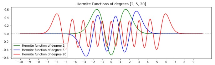
Figure 1: Plots of Hermite functions for $n=2,5,10$.

A.3 Example: Gaussian Mixture Model (GMM).

We consider the Gaussian Mixture Model with $K_{0}$ clusters centered at $\mu_{1:K_{0}}$ respectively, where

$$\mu_{k}\sim\mathcal{N}(0,\sigma_{\mu}^{2}),1\leq k\leq K_{0}.$$ (68)

The probability density of the model is given by

$$p(x;\mu_{1:K_{0}})\sim\sum_{k=1}^{K_{0}}\pi_{k}N(\mu_{z_{k}},\sigma_{x}^{2}),$$ (69)

where $\pi=(\pi_{1},\pi_{2},\dots,\pi_{K_{0}})$ is a random variable of dimension with only one non-zero entry of value $1$ in its output. Here is an example to illustrate this.

We ran this experiment: first, we sampled $N_{0}=3$ points, $\mu\sim N(0,10)$ and obtained $\mu_{1}=-18.61$, $\mu_{2}=3.81$ and $\mu_{3}=8.84$. Then we generated $n=1000$ samples by first randomly selecting an integer $i$ from $[1,2,3]$, and then drawing $x\sim N(\mu_{i},1)$. Figure 2 presents a plot of the joint distribution $p(x,\mu_{1},\mu_{2},\mu_{3})$ of this particular experiment, alongside with a normalized histogram of these $1000$ samples.

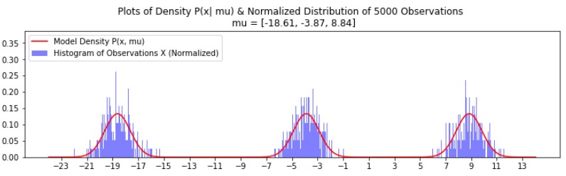
Figure 2: Example of a Mixed Gaussian Model.

In general, we are interested in the inverse problem of approximating the posterior

$$P(\mu|x_{1:n}):{\mathbb{R}^{N}}\mapsto\mathbb{R}$$ (70)

as a function of the latent variables $\mu\in{\mathbb{R}^{N}}$ given the observations $x_{1:n}$. Observe that the joint probability density function is given by

$$P(\mu_{1:K_{0}},x_{1:n})=\prod_{k=1}^{K_{0}}p(\mu_{k})\prod_{i=1}^{n}p(x_{i}|\mu_{1:K_{0}}).$$ (71)

To obtain the posterior in (70), one needs the normalizing weight $P(x_{1:n})$, which requires us to sum (71) in $k$ and integrate in $\mu_{1:K_{0}}$ . First, note that for any one sample $x$,

$$P(x|\mu_{1:K_{0}})=\displaystyle\sum_{k=1}^{K_{0}}p(x,z_{k}|\mu_{1:K_{0}})=\sum_{k=1}^{K_{0}}p(\mu_{k}|\mu_{1:K_{0}})p(x,\mu_{k})=\frac{1}{K_{0}}\sum_{k=1}^{K_{0}}p(x,\mu_{k}).$$ (72)

Then we need to integrate (72) against $d\mu_{1:K_{0}}$. That results in the following formula

$$P(x_{1:n})=\int_{\mu_{1:{K_{0}}}}\prod_{k=1}^{K_{0}}p(\mu_{k})\prod_{i=1}^{n}\left(\sum_{k=1}^{K_{0}}\displaystyle\frac{1}{K_{0}}p(x_{i},\mu_{k})\right)d\mu_{1:K_{0}}.$$ (73)

While it may be possible to compute (73) directly, the computation is far from straightforward. Furthermore, there are $K_{0}^{n}$ terms, making the computations extremely expensive as $n$ increases.

References

- Abramowitz & Stegun [1972] Abramowitz, M. and Stegun, I. A. Handbook of Mathematical Functions. Dover, 1972.
- Akhiezer [1965] Akhiezer, N. I. The Classical Moment Problem and Some Related Questions in Analysis. Dover Publications, 1965.
- Bishop [2006] Bishop, C. Pattern Recognition and Machine Learning. Springer New York, 2006.
- Blei et al. [2017] Blei, D. M., Kucukelbir, A., and MacAuliffe, J. D. Variational inference: A review for statisticians. Journal of the American Statistical Association, 112:859–877, 2017. doi: https://doi.org/10.1080/01621459.2017.1285773.
- Cools [2002] Cools, R. Advances in multidimensional integration. Journal of Computational and Applied Mathematics, 149(1):1–12, 2002.
- Deift [2000] Deift, P. Orthogonal Polynomials and Random Matrices: A Riemann-Hilbert Approach, volume 3. Courant Lecture Notes. American Mathematical Society, 2000.
- Diaconis et al. [2008] Diaconis, P., Khare, K., and Saloff-Coste, L. Gibbs sampling, exponential families and orthogonal polynomials. Statistical Science, 23(2):151–178, 2008. doi: https://doi.org/10.1214/07-STS252.
- Hastings [1970] Hastings, W. K. Monte carlo sampling methods using markov chains and their applications. Biometrika, 57(1):97–103, 1970.
- Hille [1926] Hille, E. A class of reciprocal functions. The Annals of Math., 27:427–464, 1926.
- Hinton & Camp [1993] Hinton, G. and Camp, D. V. Keeping the neural networks simple by minimizing the description length of the weights. Computational Learning Theory, pp. 5–13, 1993.
- Hoffman & Gelman [2014] Hoffman, M. D. and Gelman, A. The no-u-turn sampler: Adaptively setting path lengths in hamiltonian monte carlo. Journal of Machine Learning Research, 15:1593–1623, 2014.
- Hoffman et al. [2013] Hoffman, M. D., Blei, D. M., Wang, C., and Paisley, J. Stochastic variational inference. Journal of Machine Learning Research, 14:1307–1347, 2013.
- Huggins et al. [2017] Huggins, J. H., Adams, R. P., and Broderick, T. Pass-glm: polynomial approximate sufficient statistics for scalable bayesian glm inference. Proceedings of the 31st Annual Conference on Neural Information Processing Systems (NIPS 2017), 2017.
- Jordan et al. [1999] Jordan, M. I., Ghahramani, Z., Jaakkola, T., and Saul, L. Introduction to variational methods for graphical models. Machine Learning, 37:183–233, 1999.
- Koornwinder [2013] Koornwinder, T. Orthogonal polynomials, a short introduction. In C. Schneider, J. Bluemlein J. (eds) Computer Algebra in Quantum Field Theory. Texts & Monographs in Symbolic Computation (A Series of the Research Institute for Symbolic Computation, Johannes Kepler University, Linz, Austria), pp. 145–170. Springer, Vienna, 2013.
- Kullback & Leibler [1951] Kullback, S. and Leibler, R. On information and sufficiency. the annals of mathematical statistics. The Annals of Mathematical Statistics, 22(1):79–86, 1951.
- Lu & Darmofal [2004] Lu, J. and Darmofal, D. L. Higher-dimensional integration with gaussian weight for applications in probabilistic design. SIAM Journal of Scientific Computing, 26(2):613–624, 2004.
- Metropolis et al. [1953] Metropolis, N., Rosenbluth, A. W., Rosenbluth, M. N., and Teller, A. H. Equation of state calculations by fast computing machines. The Journal of Chemical Physics, 21, 1953.
- Millán et al. [2009] Millán, D., Rosolen, A., and Arroyo, M. Numerical integration by using local-node gauss-hermite cubature. 01 2009.
- Murphy [2012] Murphy, K. P. Machine Learning: A Probabilistic Perspective. The MIT Press, 2012.
- Nagel & Sudret [2016] Nagel, J. B. and Sudret, B. Spectral likelihood expansions for bayesian inference. Journal of Computational Physics, 309(15):267–294, 2016. doi: https://doi.org/10.1016/j.jcp.2015.12.047.
- Olver et al. [2010] Olver, F. W. J., Lozier, D. M., Boisvert, R. F., and Clark, C. W. Quadrature: Gauss-Hermite formula. Cambridge University Press, 2010.
- Opper & Saad [2001] Opper, M. and Saad, D. Advanced Mean Field Methods: Theory and Practice. Neural Information Processing series. 2001.
- Peterson & Anderson [1987] Peterson, C. and Anderson, J. R. A mean field theory learning algorithm for neural networks. Complex Systems, 1(5):995–1019, 1987.
- Riesz [1922] Riesz, M. Sur le problème des moments et le théorème de parseval correspondant. Acta Sci. Math. Szeged, 1:209–225, 1922.
- Saul & Jordan [1995] Saul, L. and Jordan, M. Exploiting tractable substructures in intractable networks. Advances in Neural Information Processing Systems, 8, 1995.
- Schmuland [1992] Schmuland, M. Dirichlet forms with polynomial domain. Math. Japonica, 37(6):1015–1024, 1992.
- Simon [1971] Simon, B. Distributions and their hermite expansions. Journal of Mathematical Physics, 12(1), 1971.
- Simon [2005] Simon, B. Orthogonal polynomials on the unit circle. Part 1 & Part 2, volume 54. American Mathematical Society, 2005.
- Soelch et al. [2016] Soelch, M., Bayer, J., Ludersdorfer, M., and van der Smagt, P. Variational inference for on-line anomaly detection in high-dimensional time series. Anamoly Detection Workshop Paper, International Conference on Machine Learning (ICML), 2016.
- Theis & Hoffman [2015] Theis, L. and Hoffman, M. D. A trust-region method for stochastic variational inference with applications to streaming data. Proceedings of the 32nd International Conference on Machine Learning, 37:2503–2511, 2015.
- vanZandt [2017] vanZandt, J. Efficient cubature rules. Electronic Transactions on Numerical Analysis, 51, 2017.
- Vinck et al. [2012] Vinck, M., Battaglia, F. P., Balakirsky, V. B., Vinck, A. J. H., and Pennartz, C. M. A. Estimation of the entropy based on its polynomial representation. Phys. Rev. E, 85(5), 2012. doi: https://doi.org/10.1103/PhysRevE.85.051139.
- Walter [1977] Walter, G. G. Properties of hermite series estimation of probability density. Annals of Statistics, 5(6):1258–1264, 1977.
- Waterhouse et al. [1996] Waterhouse, S., MacKay, D., and Robinson, T. Bayesian methods for mixtures of experts. Neural Information Processing Systems, 1996.