Graph Sequential Neural ODE Process for Link Prediction on Dynamic and Sparse Graphs

Abstract.

Link prediction on dynamic graphs is an important task in graph mining. Existing approaches based on dynamic graph neural networks (DGNNs) typically require a significant amount of historical data (interactions over time), which is not always available in practice. The missing links over time, which is a common phenomenon in graph data, further aggravates the issue and thus creates extremely sparse and dynamic graphs. To address this problem, we propose a novel method based on the neural process, called Graph Sequential Neural ODE Process (GSNOP). Specifically, GSNOP combines the advantage of the neural process and neural ordinary differential equation (ODE) that models the link prediction on dynamic graphs as a dynamic-changing stochastic process. By defining a distribution over functions, GSNOP introduces the uncertainty into the predictions, making it generalize to more situations instead of overfitting to the sparse data. GSNOP is also agnostic to model structures that can be integrated with any DGNN to consider the chronological and geometrical information for link prediction. Extensive experiments on three dynamic graph datasets show that GSNOP can significantly improve the performance of existing DGNNs and outperform other neural process variants.

1. Introduction

Graphs are ubiquitous data structures in modeling the interactions between objects. As a fundamental task in graph data mining, link prediction has been found in many real-world applications, such as social media analysis (Huo et al., 2018), drug discovery (Abbas et al., 2021), and recommender systems (Dong et al., 2012). However, data in these applications is often dynamic. For example, people interact with their friends on social media every day, and customers contiguously click or buy products in a recommender system. Therefore, it is essential to consider the nature of dynamics for accurate link prediction. As shown in Figure 1, link prediction on dynamic graphs, where interactions arrive over time, aims to predict links in the future by using historical interactions (Sankar et al., 2020; Kumar et al., 2019; Jin et al., 2022).

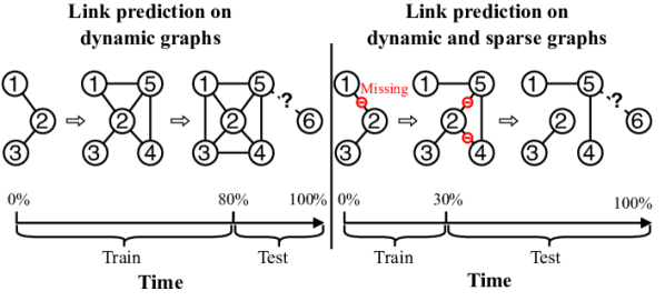
Figure 1. Comparison between link prediction on dynamic graphs and link prediction on dynamic and sparse graphs.

Recently, graph neural networks (GNNs) have shown great capacity in mining graph data (Welling and Kipf, 2016; Luo et al., 2021; Liu et al., 2021; Zheng et al., 2022b; Xiong et al., 2022; Lin et al., 2022). Under the umbrella of dynamic graph neural networks (DGNNs), several approaches have recently been proposed for predicting links on dynamic graphs (Wang et al., 2021a; Rossi et al., 2020; Wang et al., 2021b). As shown in the left panel of Figure 1, these methods typically require a large amount of historical links for training, which is unfortunately not always available (Yang et al., 2022; Zheng et al., 2022a). For instance, a new-start online shopping platform could only have few days’ user-item interactions. DGNNs trained on such limited data would be easily overfitting and cannot generalize to new links. In contrast, the platform expects models to accurately predict future interactions as early as possible, which leaves little time to collect the data. Furthermore, because the links in dynamic graphs arrive over time, the limitation of historical data in dynamic graphs would be exacerbated by the missing of interactions, resulting in extremely sparse graphs. Thus, how to enable effective link prediction on dynamic and sparse graphs (e.g., with limited historical links, as shown in the right panel of Figure 1) remains a significant challenge in this area.

Neural process (NP) (Garnelo et al., 2018b), a new family of methods, opens up a new door to dealing with limited data points in machine learning (Singh et al., 2019; Norcliffe et al., 2020; Nguyen and Grover, 2022). Based on the stochastic process, NP first draws a distribution of functions from the data by using an aggregator, and then it samples a function from the learned distribution for predictions. By defining the distribution, NP can not only readily adapt to newly observed data, but also estimate the uncertainty over the predictions, which makes models generalize to more situations, rather than overfitting to the sparse data. NP has already been applied in many applications, such as 3D rendering (Eslami et al., 2018), cold-start recommendation (Lin et al., 2021), and link prediction on static graphs (Liang and Gao, 2022).

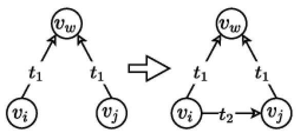
(a) Sequential and structural dependence.

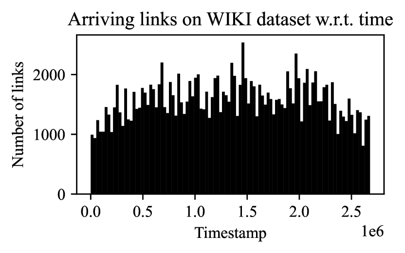
(b) Irregular arriving links in dynamic graphs.

Figure 2. (a) Sequential and structural dependence and (b) irregular arriving links in dynamic graphs.

However, NP and its variants (Kim et al., 2018; Singh et al., 2019; Cangea et al., 2022) cannot be directly applied to the link prediction on the dynamic graphs. Vanilla NP (Garnelo et al., 2018b) draws the distribution using a simple average-pooling aggregator, which ignores the sequential and structural dependence between nodes for accurate link prediction (Wang et al., 2021a; Kovanen et al., 2011; Paranjape et al., 2017). For example, as shown in the Figure 2(a), node $v_{i}$ and $v_{j}$ respectively have an interaction with node $v_{w}$ at time $t_{1}$. Therefore, node $v_{i}$ and $v_{j}$ are quite likely to interact in the future $t_{2}$. In this case, simply using average-pooling aggregator would erase the dependence and lead to a sub-optimal result. SNP (Singh et al., 2019) adopts a RNN aggregator to consider the sequential information, but it still fails to consider the derivative of the underlying distribution and uses a static distribution through time. For instance, as shown in Figure 2(b), the links in dynamic graphs arrive irregularly (Cao et al., 2021; Han et al., 2021; Wen and Fang, 2022). Additionally, an important event could lead to a large number of links occurring in a short time, which is shown by the spikes in Figure 2(b). Therefore, using a static distribution drawn from the historical data is inappropriate.

In this paper, we introduce a novel class of NP, called Graph Sequential Neural ODE Process (GSNOP) for link prediction on dynamic graphs. Specifically, GSNOP first draws a distribution of link prediction functions from historical data using a dynamic graph neural network encoder, which can be incorporated with any existing DGNN model to capture the chronological and geometrical information of dynamic graphs. Second, we propose a sequential ODE aggregator, in which we consider the function of dynamic graph link prediction as a sequence of dynamic-changing stochastic processes, and we adopt the RNN model to specify the dependence between data. To handle the irregular data, we apply the neural ordinary differential equation (ODE) (Chen et al., 2018) which is a continuous-time model defining the derivative of the hidden state with a neural network. Neural ODE is used to model the derivative of the neural process and infer the distribution in the future. In this way, we can obtain the distribution of link predict functions at any contiguous timestamp. Finally, we sample the function from the distribution for link prediction, which introduces the uncertainty over prediction results, offering a resilient way to deal with the sparse and limited data.

The main contributions of this paper are summarized as follows:

• We propose a novel class of NP, called Graph Sequential Neural ODE Process (GSNOP). To the best of our knowledge, this is the first work to apply NP for link prediction on dynamic and sparse graphs.

• We propose a dynamic graph neural network encoder and a sequential ODE aggregator, which inherits the merits of neural process and neural ODE to model the dynamic-changing stochastic process.

• We conduct extensive experiments on three public dynamic graph datasets. Experiment results show that GSNOP can significantly improve the performance of existing DGNNs on dynamic and sparse graphs.

2. Related work

In this section, we first review some representative DGNN models and then introduce the NP and its variants.

2.1. Dynamic Graph Neural Networks

Dynamic graph neural networks (DGNNs) can be roughly grouped into two categories based on the type of dynamic graphs: discrete-time dynamic graphs (DTDG) and continuous-time dynamic graphs (CTDG). DTDG-based methods model dynamic graphs as a sequence of graph snapshots. DySAT (Sankar et al., 2020) first generates node embeddings in each snapshot using an attention-based GNN, then summarize the embeddings with a Temporal Self-Attention. EvloveGCN (Pareja et al., 2020) first trains a GNN model on each snapshot and adopts the RNN to evolve the parameters of GNN to capture the temporal dynamics. Continuous-time dynamic graph (CTDG) is a more general case where links arrive with contiguous timestamps. JODIE (Kumar et al., 2019) employs two recurrent neural networks to update the node embedding by message passing. TGAT (Xu et al., 2020) proposes a temporal graph attention layer to aggregate temporal-topological neighbors. Furthermore, TGN (Rossi et al., 2020) introduces a memory module to incorporate the historical interactions. APAN (Wang et al., 2021b) decouples the message passing and memory updating process, which greatly improves the computational speed in CTDG. However, these DGNNs require sufficient training data, which largely limits their applications. MetaDyGNN (Yang et al., 2022) adopts the meta-learning framework for few-shot link prediction on dynamic graphs. But it requires new observed links to finetune the model, which shares different settings with our work.

2.2. Neural Process

Conditional neural process (CNP) (Garnelo et al., 2018a) is the first member of the NP family. CNP encodes the data into a deterministic hidden variable that parametrizes the function, which does not introduce any uncertainty. To address the limitation of CNP, neural process (NP) (Garnelo et al., 2018b) is a stochastic process that learns a latent variable to model an underlying distribution over functions, from which we can sample a function for downstream tasks. ANP (Kim et al., 2018) marries the merits of CNP and NP by incorporating the deterministic and stochastic paths in an attentive way. However, ANP could be memory-consuming when processing a long sequence, since it needs to perform self-attention on all the data points. SNP (Singh et al., 2019) further adopts RNN to consider the sequential information by modeling the changing of distribution. But it fixes the distribution in testing due to the lack of new observed data. NDP (Norcliffe et al., 2020) applies the neural ODE (Chen et al., 2018) to the decoder of neural process to consider the dynamic between data. NPs have also been applied to address many problems, such as modeling stochastic physics fields (Holderrieth et al., 2021), node classification (Cangea et al., 2022), and link prediction on static graphs (Liang and Gao, 2022). However, none of them applies NP for dynamic graph link prediction. Besides, existing NPs cannot be directly used in dynamic graphs as they ignore the sequential and structural dependence as well as the irregular data.

3. Problem Definition and Preliminary

In this section, we formally define our problem and introduce some key concepts used in this paper.

3.1. Problem Definition

Dynamic graphs can be grouped into two categories: discrete-time dynamic graphs (DTDGs) and continuous-time dynamic graphs (CTDGs). A DTDG can be defined as a sequence of graph snapshots separated by time interval: $\mathcal{G}=\{\mathcal{G}_{1},\mathcal{G}_{2},\ldots,\mathcal{G}_{T}\}$, where $\mathcal{G}_{t}=(\mathcal{V}_{t},\mathcal{E}_{t})$ is a graph taken at a discrete timestamp $t$. A CTDG is a more general case of a dynamic graph, which is constituted as a sequence of links stream $e(t)=(v_{i},v_{j},t)$ coming in over time, where $e(t)$ denotes node $v_{i}$ and $v_{j}$ has an interaction at a continuous timestamp $t$. Thus, CTDG can be formulated as $\mathcal{G}=\{e(t_{1}),e(t_{2}),\ldots\}$.

Definition 1: Link Prediction on Dynamic Graphs. Given a CTDG $\mathcal{G}$, our task is to predict links $e(t)$ at future timestamp $t>T$, using limited historical interactions $\mathcal{G}_{\leq T}=\{e(t_{1}),e(t_{2}),\ldots,e(t_{n})\}$, where $t_{i}\in[1,T]$.

3.2. Preliminary

3.2.1. Neural Ordinary Differential Equation

Neural ordinary differential equation (ODE) (Chen et al., 2018) is a continuous-time model which defines the derivative of the hidden state with a neural network. This can be formulated as

(1) $$\frac{dz(t)}{dt}=f_{ode}(z(t),t),$$

where $z(t)$ denotes the hidden state of a dynamic system at time $t$, and $f_{ode}$ denotes a neural network that describe the derivative of the hidden state w.r.t. time. Thus, the neural ODE can output the $z(t)$ at any timestamp by solving the following equation

(2) $$z(t)=z(t_{0})+\int_{t_{0}}^{t}f_{ode}(z(t_{i}),t)dt_{i}.$$

Equation 2 can be solved by using numerical ODE solver, such as Euler and fourth-order Runge-Kutta. Thus, it can be simplified as

(3) $$z(t)=ODESolve(f_{ode},z(t_{0}),t_{0},t).$$

3.2.2. Neural Process

Neural process (NP) (Garnelo et al., 2018b, a) is a stochastic process that learns an underlying distribution of the prediction function $f:X\to Y$ with limited training data. Specifically, NP defines a latent variable model using a set of context data $C=\{(x_{i},y_{i})\}_{i=1}^{n}$ to model a prior distribution $P(z|C)$. Then, the prediction likelihood on the target data $D=\{(x_{i},y_{i})\}_{i=n}^{n+m}$ is modeled as

(4) $$P(y_{n:n+m}|x_{n:n+m},C)=\int_{z}P(y_{n:n+m}|x_{n:n+m},z)P(z|C)dz.$$

We illustrate the framework of NP in Figure 3. The aim of NP is to infer the target distribution from context data. NP first draws a distribution of $f$ from the context data $C$, written as $P_{\theta}(z|C)$. By using an encoder, NP learns a low-dimension vector $r$ for each pair $(x_{C},y_{C})$ in the context data. Then, it adopts an aggregator to synthesize all the $r$ into a global representation $\mathbf{r}$, which parametrizes the distribution, formulated as $z\sim\mathcal{N}\big{(}\mu(\mathbf{r}),\sigma(\mathbf{r})\big{)}$. Last, it samples a $z$ from the distribution which is fed together with the $x_{D}\in D$ into a decoder to predict the label for target data, which is written as $P(y_{n:n+m}|x_{n:n+m},z)$. Because the true posterior is intractable, the NP is trained via variational approximation by maximizing the evidence lower bound (ELBO) as follows

(5) $$\begin{split}&logP(y_{n:n+m}|x_{n:n+m},C)\geq\\ &\mathbb{E}_{Q_{\psi}(z|C,D)}[logP_{\phi}(y_{n:n+m}|x_{n:n+m},z)]-KL\big{(}Q_{\psi}(z|C,D)||P_{\theta}(z|C)\big{)},\end{split}$$

where $Q_{\psi}(z|C,D)$ approximates the true posterior distribution also parameterized by a neural network.

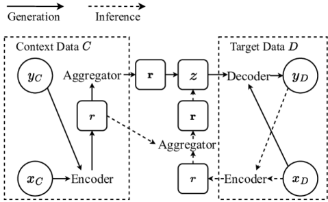
Figure 3. The framework of neural process. Circles denote the input and output data; round squares denote the latent variables.

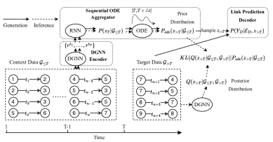
Figure 4. The framework of Graph Sequential Neural ODE Process (GSNOP) for link prediction on dynamic and sparse graphs.

4. Graph Sequential Neural ODE Process

In this section, we introduce the proposed Graph Sequential Neural ODE Process (GSNOP), which combines the merits of neural process and neural ODE to model the dynamic-changing stochastic process. GSNOP can be integrated with any dynamic graph neural network (DGNN) to simultaneously consider the chronological and geometrical information for dynamic graph link prediction. The framework of GSNOP is illustrated in Figure 4.

4.1. Setup and Framework

Given a CTDG $\mathcal{G}$, we adopt GSNOP to infer the distribution of an underlying link prediction function $f:(e(t))\to y,y\in\{0,1\}$ from context data. By specifying a timestamp $T$, we split $\mathcal{G}$ into the context data $\mathcal{G}_{\leq T}$ and target data $\mathcal{G}_{>T}$. Each $e_{C}(t)\in\mathcal{G}_{\leq T}$ occurred prior to $T$, and $e_{D}(t)\in\mathcal{G}_{>T}$ arrives when $t>T$. At testing time, we treat all the historical interactions as context data, and predict links in the future. GSNOP follows the framework of NP, thus, the encoder, aggregator, and decoder in GSNOP are defined as follows.

As shown in Figure 4, GSNOP first draws a historical distribution of $f$ from the context data $\mathcal{G}_{\leq T}$ by using a dynamic graph neural network encoder, written as $P(z_{T}|\mathcal{G}_{\leq T})$. GSNOP adopts the dynamic graph neural network to learn a low-dimension vector $r^{t}$ for each link in the context data. Then, it adopts an sequential ODE aggregator to synthesize all the $r^{t}$ into a global representation $\mathbf{r}_{T}$, which parametrizes the distribution $P(z_{T}|\mathcal{G}_{\leq T})$, formulated as $z_{T}\sim\mathcal{N}\big{(}\mu(\mathbf{r}_{T}),\sigma(\mathbf{r}_{T})\big{)}$. Following, GSNOP applies the neural ODE on the $P(z_{T}|\mathcal{G}_{\leq T})$ to infer the distribution in the future $>T$, written as $P_{ode}(z_{>T}|\mathcal{G}_{\leq T})$ Last, GSNOP sampled a $z_{>T}$ from the future distribution which is fed together with the $e_{D}(t)\in\mathcal{G}_{>T}$ into a link prediction decoder to predict the links in target data, which is formulated as $f(e_{D}(t),z_{>T})\to y_{T}$. Each component is introduced in detail as follows.

4.2. Dynamic Graph Neural Network Encoder

The encoder is applied to each pair $(e_{C}(t),y_{C})$ in the context data, where $y_{C}$ denotes the existence of the links. It tries to capture the connection between $e_{C}(t)$ and $y_{C}$ to infer the distribution of link prediction function $f$. Link prediction on dynamic graph has been studied for years. Previous research has shown that the dynamic graph neural networks (DGNNs) have great potential to capture the chronological and geometrical information for dynamic graph link prediction (Xu et al., 2020; Rossi et al., 2020). Therefore, we adopt the DGNNs as the encoder of GSNOP.

Given a pair $(e_{C}(t),y_{C})$, we first adopt a DGNN to generate the representation $h^{t}$ of nodes $v_{i},v_{j}\in e_{C}(t)$, which is formulated as

(6) $$h^{t}=\text{DGNN}\Big{(}h^{t-1},agg\big{(}N_{<t}(v)\big{)}\Big{)},$$

where $h^{t-1}$ denotes the representation of node $v$ in the last timestamp, $N_{<t}(v)$ denotes a set of nodes that interacted with $v$ in previous timestamps, and $agg(\cdot)$ denotes the aggregation operation defined by DGNN. Equation 6 can be written as $\text{DGNN}(v,N_{<t}(v))$ for simplification. We can use arbitrary DGNN to consider the dynamic and graph structure information for a given node.

Then, we use a MLP to encode each pair $(e_{C}(t),y_{C})$ into a representation $r^{t}$, which is formulated as

(7) $$r^{t}=\text{MLP}\Big{(}h_{i}^{t}||h_{j}^{t}||y\Big{)}+t_{emb},y=\left\{\begin{aligned} 1,e_{C}(t)\in\mathcal{G}_{\leq T}\\ 0,e_{C}(t)\notin\mathcal{G}_{\leq T}\end{aligned}\right.,$$

where $||$ denotes the concatenation operation, $y$ denotes the existence of the link between $v_{i}$ and $v_{j}$ in the context data, and $t_{emb}$ denotes the time embedding (Xu et al., 2020) sharing the same dimension with $r^{t}$ that can be learned during the training.

4.3. Sequential ODE Aggregator

The aggregator summarizes encoder outputs into a global representation $\mathbf{r}_{T}$ that parametrizes latent distribution $z_{T}\sim\mathcal{N}\big{(}\mu(\mathbf{r}_{T}),\sigma(\mathbf{r}_{T})\big{)}$. Originally, NP (Chen et al., 2018) adopts a simple average-pooling aggregator, which is formulated as

(8) $$\mathbf{r}_{T}=\frac{1}{|\mathcal{G}_{\leq T}|}\sum_{e_{C}(t)\in\mathcal{G}_{\leq T}}r^{t}.$$

However, it fails to consider the sequential and structural dependence between nodes in dynamic graphs.

Vanilla NP assumes that data in the context data is i.i.d., thus it adopts a simple average-pooling aggregator to define the joint distribution $P(z_{T}|\mathcal{G}_{\leq T})$. However, in dynamic graphs, we need to consider the sequential and structural dependence between nodes for accurate link prediction (Wang et al., 2021a; Kovanen et al., 2011; Paranjape et al., 2017). In this case, simply using average-pooling aggregator would erase the dependence between $e_{C}(t)\in\mathcal{G}_{\leq T}$ and lead to a sub-optimal result.

To consider the sequential and structural dependence, inspired by Sequential Neural Process (SNP) (Singh et al., 2019), we consider the dynamic graph link prediction function as a sequence of dynamic-changing stochastic processes $\{\mathcal{P}_{1},\ldots,\mathcal{P}_{T}\}$. At each timestamp $t$, we can observe a set of context data $\{(e(t),y)\in\mathcal{G}_{t}\}$, where $\mathcal{G}_{t}$ might differ over time. We can infer a distribution $\mathcal{P}_{t}$ by using all the historical data $\mathcal{G}_{\leq t}$, which can be formulated as

(9) $$\mathcal{P}_{t} =P(z_{t}|\mathcal{G}_{\leq t})=P(z_{t}|\mathcal{P}_{t-1},\mathcal{G}_{t}).$$

Because, $\mathcal{P}_{t-1}$ denotes the distribution drawn from the $\mathcal{G}_{<t}$. By modeling the changing of process $\mathcal{P}_{t-1}\to\mathcal{P}_{t}$, we can consider the dependence among context data. Thus, we adopt a RNN model to specify the state transition model in Eq. (9), which is formulated as

(10) $$\mathbf{r}_{t}=\text{RNN}(\mathbf{r}_{t-1},\mathcal{G}_{t}),t>1,$$

where $\mathbf{r}_{1}$ is computed by averaging $r^{1}$ generated from $\mathcal{G}_{1}$. By using the RNN aggregator, we can obtain the $\mathbf{r}_{T}$ from the representation of context data $\{r^{t_{1}},\ldots,r^{T}\}$ and define the distribution $P(z_{T}|\mathcal{G}_{\leq T})$. But, it still fails to consider the derivative of the underlying distribution.

In vanilla NP, it infers the distribution of link prediction function $P(z_{T}|\mathcal{G}_{\leq T})$ from historical context data, and fixes it for future link prediction. However, in dynamic graphs, the links arrive in different frequencies (Cao et al., 2021; Han et al., 2021; Wen and Fang, 2022). Therefore, it is inappropriate to use a static distribution over time, although we can incorporate the new-coming links into the context data and update the distribution by using Eq. 10. In most cases, it is infeasible to obtain the links in the future. As a result, we need to consider the derivative of distribution over time to deal with irregular data.

Recently, neural ordinary differential equation (ODE) (Chen et al., 2018) has shown great power in dealing irregular time series data (Rubanova et al., 2019). Thus, in GSNOP, we apply the neural ODE to model the derivative of neural process and infer the distribution in the future $P_{ode}(z_{>T}|\mathcal{G}_{\leq T})$.

Given a distribution $P(z_{T}|\mathcal{G}_{\leq T})$ drawn from context data $\mathcal{G}_{\leq T}$, it is parameterized by the global latent variable $\mathbf{r}_{T}$. We apply the neural ODE on the $\mathbf{r}_{T}$ to obtain the latent variable at any future time $>T=T+\triangle t$, which is formulated as

(11) $$\mathbf{r}_{>T}=\mathbf{r}_{T}+\int_{T}^{T+\triangle t}f_{ode}(\mathbf{r}_{t},t)dt,$$

where $f_{ode}$ denotes the neural ODE function, which is formulated as

(12) $$f_{\theta}(\mathbf{r}_{t},t)=Tanh(MLP(\mathbf{r}_{t}+t_{emb})).$$

We use the $Tanh$ as the activation function to keep from gradient exploration.

After obtaining the $r_{>T}$, the distribution parameterized by $\mathbf{r}_{>T}$ can be considered as a Gaussian distribution $\mathcal{N}\big{(}\mu(\mathbf{r}_{>T}),\sigma(\mathbf{r}_{>T})\big{)}$, where the mean $\mu(\mathbf{r}_{>T})$ and variance $\sigma(\mathbf{r}_{>T})$ are formulated as

(13) $$\chi=\text{MLP}(\mathbf{r}_{>T}),$$

(14) $$\mu(\mathbf{r}_{>T})=ReLU(\text{MLP}(\chi)),$$

(15) $$\sigma(\mathbf{r}_{>T})=0.1+0.9*Sigmoid(\text{MLP}(\chi)).$$

4.4. Link Prediction Decoder

The decoder is considered as the underlying link prediction function $f(e(t),z)\to y$. Given two nodes $v_{i}$ and $v_{j}$ at time $t$ to be predicted, $f$ can be formulated as

(16) $$h_{i}^{t}=\text{DGNN}(v_{i},N_{<t}(v_{i})),h_{j}^{t}=\text{DGNN}(v_{j},N_{<t}(v_{i}))$$

(17) $$\text{Sample }z_{>T}\sim\mathcal{N}\big{(}\mu(\mathbf{r}_{>T}),\sigma(\mathbf{r}_{>T})\big{)}$$

(18) $$\widetilde{h_{i}^{t}}=ReLU(\text{MLP}(h_{j}^{t}||z_{>T})),\widetilde{h_{j}^{t}}=ReLU(\text{MLP}(h_{j}^{t}||z_{>T})),$$

(19) $$\hat{y}=Sigmoid\big{(}\text{MLP}(\widetilde{h_{i}^{t}}||\widetilde{h_{j}^{t}})\big{)},$$

where $\hat{y}$ denotes the prediction result.

The decoder is conditioned on the variable $z_{>T}$ sampled from the distribution. This injects the uncertainty into the prediction results, making GSNOP generalize to more situations, even with limited data. In addition, as more data observed, the distribution could be refined and provide more accurate predictions, which is demonstrated in section 5.5.

4.5. Optimization

Given the context data $\mathcal{G}_{\leq T}$ and target data $\mathcal{G}_{>T}$, the object of GSNOP is to infer the distribution $P(z_{>T}|\mathcal{G}_{\leq T})$ from the context data that minimize the prediction loss on the target data. Therefore, the generation process of GSNOP can be written as

(20) $$P(Y_{D},z_{>T}|\mathcal{E}_{D},\mathcal{G}_{\leq T})=P(z_{>T}|\mathcal{G}_{\leq T})\prod_{e_{D}(t)\in\mathcal{E}_{D}}P\big{(}y_{D}|f(e_{D}(t),z_{>T})\big{)},$$

where $f$ is the link prediction decoder, and $\mathcal{E}_{D}=\{e_{D}(t)\in\mathcal{G}_{>T}\}$ denotes the links to be predicted in the target data.

Since the decoder $f$ is non-linear, it can be trained using an amortised variational inference procedure. We can optimize the evidence lower bound (ELBO) to minimize the prediction loss on target data given the context data $logP(Y_{D}|\mathcal{E}_{D},\mathcal{G}_{\leq T})$, which can be derivate as

(21) $$logP(Y_{D}|\mathcal{E}_{D},\mathcal{G}_{\leq T})=\int_{z}Q(z_{>T})log\frac{P(Y_{D},z_{>T}|\mathcal{E}_{D},\mathcal{G}_{\leq T})}{P(z_{>T}|\mathcal{G}_{\leq T})},$$

(22) $$\geq\int_{z}Q(z_{>T})log\frac{P(Y_{D},z_{>T}|\mathcal{E}_{D},\mathcal{G}_{\leq T})}{Q(z_{>T})},$$

(23) $$=\mathbb{E}_{Q(z_{>T})}log\frac{P(Y_{D},z_{>T}|\mathcal{E}_{D},\mathcal{G}_{\leq T})}{Q(z_{>T})},$$

(24) $$=\mathbb{E}_{Q(z_{>T})}[logP(Y_{D}|\mathcal{E}_{D},z_{>T})+log\frac{P(z_{>T}|\mathcal{G}_{\leq T})}{Q(z_{>T})}],$$

(25) $$=\mathbb{E}_{Q(z_{>T})}[logP(Y_{D}|\mathcal{E}_{D},z_{>T})]-KL\big{(}Q(z_{>T})||P(z_{>T}|\mathcal{G}_{\leq T})\big{)},$$

where $Q(z_{>T})$ denotes the true posterior distribution of $z_{>T}$.

Thus, we can obtain the final ELBO loss as

(26) $$\begin{split}\mathcal{L}_{ELBO}=&\mathbb{E}_{Q_{\psi}(z_{>T}|\mathcal{G}_{\leq T},\mathcal{G}_{>T})}[logP_{\phi}(Y_{D}|\mathcal{E}_{D},z_{>T})]\\ &-KL\big{(}Q_{\psi}(z_{>T}|\mathcal{G}_{\leq T},\mathcal{G}_{>T})||P_{ode}(z_{>T}|\mathcal{G}_{\leq T})\big{)}.\end{split}$$

where $logP_{\phi}(Y_{D}|\mathcal{E}_{D},z_{>T})=\sum_{e_{D}(t)\in\mathcal{E}_{D}}P_{\phi}(y_{D}|e_{D}(t),z_{>T})$ denotes the prediction loss on the target data and $P_{\phi}$ is parameterized by the decoder. The $Q(z_{>T})$ is approximated by the variational posterior $Q_{\psi}(z_{>T}|\mathcal{G}_{\leq T},\mathcal{G}_{>T})$ calculated by the encoder and RNN aggregator, formulated as

(27) $$r^{t}=\text{DGNN Encoder}\big{(}(e_{D}(t),y_{D})\big{)},(e_{D}(t),y_{D})\in\mathcal{G}_{>T},$$

(28) $$\mathbf{r^{\prime}}_{>T}=\text{RNN}(\mathbf{r}_{T},r^{t}),$$

(29) $$Q_{\psi}(z_{>T}|\mathcal{G}_{\leq T},\mathcal{G}_{>T})=\mathcal{N}\big{(}\mu(\mathbf{r^{\prime}}_{>T}),\sigma(\mathbf{r^{\prime}}_{>T})\big{)}.$$

The prior $P(z_{>T}|\mathcal{G}_{\leq T})$ is approximated by the neural ODE in Eq. 11, written as $P_{ode}(z_{>T}|\mathcal{G}_{\leq T})$. By minimizing the KL divergence between variational posterior and the prior $P_{ode}(z_{>T}|\mathcal{G}_{\leq T})$, it encourages the neural ODE to learn the derivative of distribution and infer the distribution in the future. Extended derivation of Eq. 26 can be found in the supplementary file of this link.

Noticeably, unlike neural ODE process (Norcliffe et al., 2020) which applies neural ODE on the decoder, GSNOP applies neural ODE to infer the distribution of function at any contiguous timestamp. This is more suitable for the dynamic-changing stochastic process modeled for dynamic graph link prediction.

Testing. At test time, given a set of historical interactions $\mathcal{G}_{\leq T}$, we treat them as the context data and draw a global representation $\mathbf{r}_{T}$ using the DGNN encoder as well as RNN aggregator. Then, given a link $e(T+\triangle t)$ to be predicted, we apply the neural ODE to infer the distribution at future, formulated as

(30) $$r_{>T}=ODESolve(f_{ode},r_{T},T,T+\triangle t),$$

(31) $$\text{Sample }z_{>T}\sim\mathcal{N}\big{(}\mu(\mathbf{r}_{>T}),\sigma(\mathbf{r}_{>T})\big{)}.$$

Last, we use the decoder to predict the link $f(e(T+\triangle t),z_{>T})\to y$.

Given a CTDG containing $n$ links in context data and $m$ links to be predicted in the target data, the time complexity of GSNOP is $O(n+m)$ since model need to encode each link in the context data and predict each target link. This shows that GSNOP scales well with the size of the input. At testing time, we also batch the samples by using the dummy variable trick (Chen et al., 2020) to speed up the integration in neural ODE.

5. Experiment

5.1. Datasets

We conduct experiments on three widely used CTDG datasets: WIKI (Rossi et al., 2020), REDDIT (Rossi et al., 2020), and MOOC (Kumar et al., 2019). Following the settings of the previous work (Xu et al., 2020), we focus on the task of predicting links in the future using limited historical interactions. Intuitively, with the links coming over time, the CDTG would become denser. To simulate different levels of graph sparsity, we split the CDTG chronologically by timestamps in the entire duration with two ratios, 30%-20%-50% and 10%-10%-80% for training, validation, and testing. The datasets with different splits are labeled by their training ratio (e.g., WIKI_0.3 and WIKI_0.1). The sparsity of graphs can be quantified by the density score, calculated as $\frac{2|\mathcal{E}|}{|\mathcal{V}|(|\mathcal{V}|-1)}$, where $|\mathcal{E}|$ and $|\mathcal{V}|$ denote the number of links and nodes in the training set. The statistics of the datasets is shown in Table 1.

Table 1. Dataset statistics. The max($t$) column shows the maximum timestamps of links. The $d_{e}$ denotes the dimension of link features. Density (0.3) and Density (0.1) respectively denote the density scores of CDTG under different splits.

Dataset	$|\mathcal{V}_{all}|$	$|\mathcal{E}_{all}|$	max($t$)	$d_{e}$	Density (0.3)	Density (0.1)
WIKI	9,228	157,474	2.70E+06	172	1.03E-03	2.90E-04
REDDIT	10,985	672,447	2.70E+06	172	3.18E-03	1.01E-03
MOOC	7,047	411,749	2.60E+06	128	4.03E-03	1.52E-03

5.2. Baselines

Since GSNOP is agnostic to model structure, we choose several state-of-the-art DGNN as baselines (i.e., JODIE (Kumar et al., 2019), DySAT (Sankar et al., 2020), TGAT (Xu et al., 2020), TGN (Rossi et al., 2020), and APAN (Wang et al., 2021b)). Detailed introductions of these DGNNs can be found in section 2.1. To demonstrate the effectiveness of GSNOP, we adopt these DGNNs respectively as the encoder in GSNOP to illustrate the performance improved by GSNOP. In addition, we also select other neural process variants (i.e., Neural Process (NP) (Garnelo et al., 2018b), Conditional Neural Process (Garnelo et al., 2018a) and Sequential Neural Process (SNP) (Singh et al., 2019)) to demonstrate the superiority of GSNOP.

5.3. Settings

In experiments, we adopt the average precision (AP) and mean reciprocal rank (MRR) as evaluation metrics. To fairly evaluate the performance in sparse settings (Yokoi et al., 2017), we randomly select 50 negative links for each positive link in the evaluation stage.

For each DGNN baseline, we set the layer of the GNN to 2 and the number of neighbors per layer to 10. The memory size for APAN is set to 10, while 1 for JODIE and TGN. For snapshot-based DySAT, we set the number of snapshots to 3 with the duration of each snapshot to be 10,000 seconds. For all methods, the dropout rate is swept from {0.1,0.2,0.3,0.4,0.5}, and the dimension of output node embeddings is set to 100. We use the function in section 4.4 to predict links.

For GSNOP, the dimension of $r^{t}$, $t_{emb}$, and $z$ are all set to 256. The Monte Carlo sampling size for approximating $\mathbb{E}_{Q_{\psi}(z_{>T}|G_{\leq T},G_{>T})}$ in $\mathcal{L}_{ELBO}$ is set to 10. We use GRU (Chung et al., 2014) as the RNN aggregator and choose 5 order Runge-Kutta of Dormand-Prince-Shampine (Calvo et al., 1990) as the ODE solver with relative tolerance set to $1e-5$ and absolute tolerance set to $1e-7$. We use Adam as the optimizer, and the learning rate is set to 0.00001. The implementation of GSNOP is available at this link .

Table 2. Experiments results on WIKI, REDDIT, and MOOC datasets.

Method	WIKI_0.3		REDDIT_0.3		MOOC_0.3		WIKI_0.1		REDDIT_0.1		MOOC_0.1
	AP	MRR	AP	MRR	AP	MRR	AP	MRR	AP	MRR	AP	MRR
JODIE	0.3329	0.5595	0.6320	0.8101	0.6690	0.8802	0.1820	0.4476	0.3324	0.6401	0.7100	0.9063
JODIE+GSNOP	0.4258	0.6086	0.8171	0.8922	0.6716	0.8853	0.2979	0.5273	0.4705	0.7260	0.7196	0.9066
DySAT	0.3881	0.6680	0.5705	0.7887	0.6441	0.8807	0.3872	0.6601	0.5353	0.7853	0.6705	0.8968
DySAT+GSNOP	0.5816	0.7716	0.7406	0.8443	0.6528	0.8811	0.3910	0.6628	0.5738	0.7887	0.6718	0.8971
TGAT	0.3253	0.5229	0.8343	0.8797	0.5183	0.7828	0.2766	0.4638	0.4833	0.6523	0.1919	0.4228
TGAT+GSNOP	0.3701	0.5348	0.8395	0.8820	0.5448	0.7905	0.3366	0.4961	0.5240	0.6807	0.1874	0.4581
TGN	0.5541	0.7788	0.7621	0.8587	0.7200	0.9007	0.5676	0.7631	0.6749	0.8029	0.7677	0.9087
TGN+GSNOP	0.6633	0.7816	0.8307	0.8935	0.7445	0.9117	0.6568	0.7674	0.7148	0.8263	0.7714	0.9174
APAN	0.2431	0.5496	0.6166	0.7799	0.6601	0.8774	0.0504	0.1857	0.5601	0.7415	0.7016	0.8967
APAN+GSNOP	0.4570	0.6918	0.7119	0.8560	0.6614	0.8790	0.1996	0.5607	0.6126	0.7606	0.7052	0.8982

Table 3. Experiments results on WIKI and REDDIT w.r.t. different sample ratios.

Dataset	WIKI_0.3										REDDIT_0.3
Sample Ratio	100%		80%		50%		20%		10%		100%		80%		50%		20%		10%
Method	AP	MRR	AP	MRR	AP	MRR	AP	MRR	AP	MRR	AP	MRR	AP	MRR	AP	MRR	AP	MRR	AP	MRR
JODIE	0.3329	0.5595	0.2804	0.5046	0.1464	0.3950	0.0300	0.1598	0.0238	0.1289	0.1820	0.4476	0.1966	0.4574	0.1215	0.3959	0.0222	0.1207	0.0246	0.1366
JODIE+GSNOP	0.4258	0.6086	0.3177	0.5171	0.2666	0.4738	0.1845	0.4192	0.0663	0.2784	0.2979	0.5273	0.2382	0.4816	0.1824	0.4157	0.1017	0.3302	0.0406	0.2214
DySAT	0.3881	0.6680	0.3856	0.6691	0.3873	0.6676	0.3870	0.6610	0.3121	0.6403	0.3872	0.6601	0.3179	0.6244	0.3165	0.6385	0.3161	0.6450	0.3118	0.6413
DySAT+GSNOP	0.5816	0.7716	0.5539	0.6691	0.4349	0.4349	0.3900	0.6615	0.3159	0.6419	0.3910	0.6628	0.3870	0.6612	0.3174	0.6441	0.3229	0.6534	0.3050	0.6409
TGAT	0.3253	0.5229	0.3274	0.5238	0.2717	0.4769	0.2573	0.4783	0.2536	0.4722	0.2766	0.4638	0.2782	0.4861	0.1215	0.3830	0.1356	0.3545	0.1114	0.3567
TGAT+GSNOP	0.3701	0.5348	0.3594	0.5281	0.3630	0.5314	0.3371	0.4955	0.2882	0.4571	0.3366	0.4961	0.3420	0.5055	0.3055	0.4586	0.2045	0.3731	0.0600	0.2408
TGN	0.5541	0.7788	0.5327	0.7560	0.5084	0.7341	0.4361	0.6809	0.4918	0.6831	0.5676	0.7631	0.3576	0.6632	0.3633	0.6576	0.4160	0.6604	0.0312	0.1681
TGN+GSNOP	0.6633	0.7816	0.6395	0.7762	0.6179	0.7685	0.5535	0.7094	0.5566	0.6968	0.6568	0.7674	0.6435	0.7679	0.5506	0.7330	0.5094	0.6868	0.3974	0.6374
APAN	0.2431	0.5496	0.2198	0.5374	0.1768	0.5179	0.0928	0.2524	0.0431	0.1969	0.0504	0.1857	0.0547	0.1900	0.0631	0.2442	0.0367	0.1388	0.0331	0.1226
APAN+GSNOP	0.4570	0.6918	0.4363	0.6821	0.2068	0.5311	0.0735	0.2797	0.0588	0.2128	0.1996	0.5607	0.0638	0.1958	0.0644	0.3075	0.0430	0.1964	0.0288	0.1173
Dataset	WIKI_0.1										REDDIT_0.1
Sample Ratio	100%		80%		50%		20%		10%		100%		80%		50%		20%		10%
Method	AP	MRR	AP	MRR	AP	MRR	AP	MRR	AP	MRR	AP	MRR	AP	MRR	AP	MRR	AP	MRR	AP	MRR
JODIE	0.6320	0.8101	0.6118	0.8085	0.4374	0.7306	0.3391	0.6597	0.2984	0.5949	0.3324	0.6401	0.3183	0.6307	0.3134	0.6179	0.3156	0.6226	0.0380	0.1854
JODIE+GSNOP	0.8171	0.8922	0.7543	0.8617	0.4860	0.7546	0.3907	0.6806	0.3130	0.6140	0.4705	0.7260	0.4428	0.6653	0.3637	0.6585	0.3760	0.6681	0.0635	0.2436
DySAT	0.5705	0.7887	0.5714	0.7888	0.5732	0.7925	0.5786	0.7919	0.5751	0.7872	0.5353	0.7853	0.5458	0.7795	0.5371	0.7845	0.5568	0.7818	0.5598	0.7798
DySAT+GSNOP	0.7406	0.8443	0.7281	0.8390	0.6106	0.7977	0.6166	0.7982	0.6110	0.7964	0.5738	0.7887	0.5755	0.7945	0.5721	0.7955	0.5786	0.7954	0.5947	0.7942
TGAT	0.8343	0.8797	0.8193	0.8702	0.8074	0.8604	0.7775	0.8490	0.4192	0.6160	0.4833	0.6523	0.4885	0.6512	0.3783	0.5651	0.2129	0.4615	0.2056	0.4518
TGAT+GSNOP	0.8395	0.8820	0.8426	0.8839	0.8168	0.8757	0.7917	0.8544	0.4513	0.6295	0.5240	0.6807	0.5247	0.6862	0.4181	0.6041	0.3709	0.5667	0.2426	0.4684
TGN	0.7621	0.8587	0.7118	0.8471	0.7247	0.8424	0.3549	0.6572	0.3005	0.5934	0.6749	0.8029	0.6631	0.7917	0.5958	0.7502	0.2403	0.5312	0.2219	0.5152
TGN+GSNOP	0.8307	0.8935	0.8235	0.8967	0.7567	0.8444	0.5923	0.7941	0.5024	0.7373	0.7148	0.8263	0.6995	0.8095	0.5134	0.7494	0.2701	0.5458	0.1929	0.4410
APAN	0.6166	0.7799	0.4879	0.7527	0.4914	0.7306	0.4637	0.7294	0.4943	0.7148	0.5601	0.7415	0.5733	0.7407	0.2991	0.6973	0.3566	0.6761	0.3586	0.6677
APAN+GSNOP	0.7119	0.8560	0.7229	0.8498	0.5370	0.7500	0.4865	0.7331	0.4925	0.7133	0.6126	0.7606	0.6131	0.7418	0.4157	0.7403	0.4397	0.6831	0.3756	0.6823

5.4. Performance Comparison

In this section, we evaluate the performance of GSNOP on different datasets. The results are shown in Table 2. From the results, we can see that GSNOP enables to improve the performance of all the baselines with respect to different datasets and training ratios.

Specifically, when the historical training data is sufficient, all DGNNs achieve relatively good performance in WIKI_0.3, REDDIT_0.3, and MOOC_0.3. However, when training data is limited, the performance of some baselines drops significantly (e.g., JODIE, TGAT, and APAN). The possible reason is that these DGNNs use historical data to generate node embeddings. When data is limited, the quality of the generated embeddings cannot be guaranteed. Thus, it is inaccurate to use such embeddings for link prediction directly. In addition, the data distribution of the testing set could be diverse from the training set. This would lead the model overfit to the historical data and cannot generalize to the future links. The performances between MOOC_0.3 and MOOC_0.1 are similar. This is because MOOC is a denser CTDG with short duration. Thus, most DGNNs perform well in this dataset.

In GSNOP, we model the distribution of function from the historical data by learning a latent variable. This variable introduces a global view of knowledge, from which we can sample a link prediction function rather than only use the node embeddings. Besides, the distribution introduces uncertainty over prediction results. In this way, GSNOP can generalize to more situations instead of overfitting to the training data. Last, by adopting the neural ODE, GSNOP enables to infer the distribution in the future with a small amount of historical data. Noticeably, the improvement of GSNOP is sometimes limited (e.g., results in MOOC_0.1). The possible reason is that GSNOP learns the latent variable by optimizing the evidence lower bound. This does not always result in a meaningful latent variable that parametrizes the distribution (Alemi et al., 2018; Nguyen and Grover, 2022). We will leave this for future exploration.

5.5. Performance at Different Levels of Sparsity

In the real-world, we might only observe partial links for an underlying CTDG, which aggravates the sparsity. To further demonstrate the performance improvement under different sparsity, we sample subsets of training links from the original training set with various sample ratios, while leave the validation and test set unchanged. For instance, the 30% sample ratio in WIKI_0.3 denotes that we randomly mask 70% of links in the training set and use the remaining 30% links for training. The density score of the sampled dataset can be calculated by multiplying the sample ratio and the density of the original dataset. We sweep the sample ratio from 100% to 10%. The results are shown in Table 3.

Table 4. Comparing with other neural process variants.

Method	WIKI_0.3										WIKI_0.1
	Origin		NP		CNP		SNP		GSNOP		origin		NP		CNP		SNP		GSNOP
	AP	MRR	AP	MRR	AP	MRR	AP	MRR	AP	MRR	AP	MRR	AP	MRR	AP	MRR	AP	MRR	AP	MRR
JODIE	0.3868	0.6241	0.4063	0.6118	0.3255	0.5943	0.4173	0.6023	0.4258	0.6086	0.1946	0.4741	0.2223	0.4699	0.1201	0.3609	0.2804	0.5149	0.2979	0.5273
DySAT	0.3757	0.6727	0.4226	0.6818	0.3494	0.6552	0.4199	0.6821	0.5816	0.7716	0.3152	0.6461	0.3151	0.6452	0.3482	0.6386	0.3874	0.6612	0.3910	0.6628
TGAT	0.3277	0.5171	0.3456	0.5147	0.2881	0.4680	0.3462	0.5173	0.3701	0.5348	0.2766	0.4638	0.3051	0.4704	0.2407	0.4474	0.2996	0.4646	0.3366	0.4961
TGN	0.5611	0.7789	0.6632	0.7837	0.6539	0.7766	0.6577	0.7809	0.6633	0.7816	0.5778	0.7750	0.6362	0.7617	0.5703	0.7347	0.6479	0.7656	0.6568	0.7674
APAN	0.2191	0.5085	0.0784	0.2701	0.0987	0.3195	0.1090	0.3503	0.4570	0.6918	0.1598	0.5251	0.0820	0.3115	0.0836	0.2837	0.1135	0.3995	0.1996	0.5607

From the results, we can see that GSNOP outperforms the baselines under different levels of sparsity. Specifically, with the sample ratio decreasing, the performance of each DGNN also decreases. This is because when the training data is sparse, the model cannot capture enough interactions for link prediction. However, with GSNOP, we can define the distribution with limited interactions to estimate the underlying graph. Thus, it can better handle the sparsity situation. In addition, GSNOP can incorporate new observations to enhance the distribution. With the sample ratio increasing from 10%-100%, the improvement bought by GSNOP increases. The reason is that by adding new observed links into the latent variable, GSNOP enables to more accurately define the distribution of function with the help of DGNN encoder and RNN aggregator.

5.6. Ablation Study

In this section, we compare our GSNOP with other neural process variants (i.e., vanilla neural process (NP) (Garnelo et al., 2018b), conditional neural process (Garnelo et al., 2018a) and sequential neural process (SNP) (Singh et al., 2019)) to show the superiority of our method in dynamic graph link prediction. For each variant, we use our dynamic graph neural network encoder and link prediction decoder but maintain their original way of generating the distribution. The results in Table 4 would help to demonstrate the effectiveness of our sequential ODE aggregator.

From the results, we can see that GSNOP performs better than other neural process variants. NP is the original version of neural process. Since it ignores the sequential and structural dependence, NP has the minimum improvement. Compared with other variants, CNP achieves the worst performance. The reason is that CNP is a deterministic version of neural process. Instead of learning the latent variable, CNP directly models the distribution conditioned on the context data, which could be inaccurate when the context data is limited. SNP adopts the RNN as the aggregator, which considers the sequential dependence. However, it fails to capture the distribution derivative, making SNP unable to handle irregular data. GSNOP incorporates both the RNN aggregator and neural ODE, which simultaneously exploits the sequential information and enables inferring the distribution at any timestamps. Thus, GSNOP achieves the best results among all the variants.

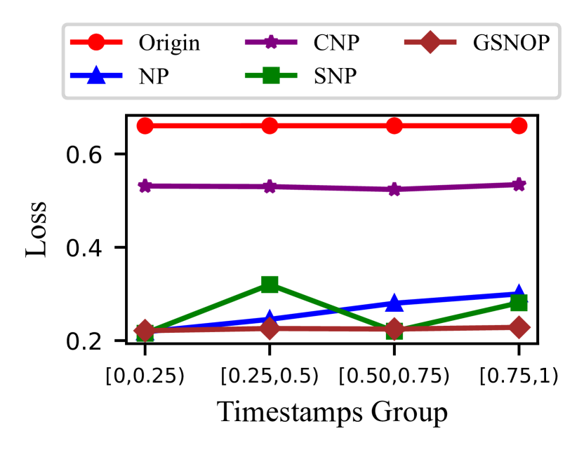
(a) Prediction loss of each group.

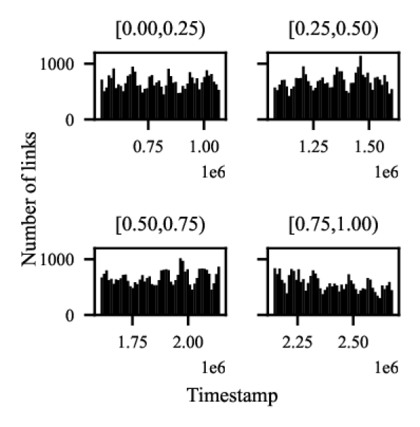
(b) Arriving links of each group.

Figure 5. (a) Prediction loss and (b) arriving links of each group.

To further demonstrate the effectiveness of Sequential ODE aggregator, we split links in the test set of WIKI_0.1 chronologically into four groups based on their timestamps. For example, the group [0, 0.25) denotes the links between $0$ and $0.25*max(t)$ in the test set. The prediction loss of each group with DySAT as the encoder is shown in Figure 5(a). From the results, we can see that Origin and CNP have relatively high losses across different groups. Due to the ignoring of sequential dependence, NP cannot infer the distribution in the future. Thus, the loss of NP increases with the timestamps. Despite SNP capturing the sequential information, it still fails to address the irregular data. As shown in Figure 5(b), there is a high spike in group [0.25, 0.5), and the arriving links are decreasing in group [0.75, 1.00). Thus, the losses of SNP are higher in these irregular groups. With the help of the sequential ODE aggregator, GSNOP models the distribution derivative and maintain relatively low losses across different timestamps.

5.7. Parameters Analysis

We investigate two critical hyperparameters (i.e., learning rate and the dimension of $z$) in Figure 6. From the results, we can see that the learning rate could severely impact the performance of GSNOP. This is because GSNOP adopts the dummy variable trick (Chen et al., 2020) to speed up the neural ODE. However, this will incur the gradient explosion problem when integrating in a large time period. Thus, we need to select a relatively small learning rate (i.e., $1e-5$) to avoid gradient explosion. However, a too small learning rate also causes underfitting and leads the performance drops. With the dimension of $z$ increasing, the performance of GSNOP improves and reaches the best at 256. The reason is that a small dimension of $z$ cannot well model the stochastic of distribution, but an over large dimension would also introduce noises when optimizing the evidence lower bound, which deteriorates the performance.

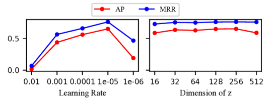
Figure 6. Parameter sensitivity w.r.t. different learning rate and the dimension of $z$.

6. Conclusion

In this paper, we propose a novel NP named GSNOP for link prediction on dynamic graphs. We first specify a dynamic graph neural network encoder to capture the chronological and geometrical information of dynamic graphs. Then, we propose a sequential ODE aggregator, which not only considers the sequential dependence among data but also learns the derivate of the neural process. In this way, it can better draw the distribution from limited historical links. We conduct extensive experiments on three public datasets, and the results show that GSNOP can significantly improve the link prediction performance of DGNNs in dynamic and sparse graphs. Experiment results comparing with other NP variants further demonstrate the effectiveness of our method.

7. Acknowledge

This work is supported by an ARC Future Fellowship (No. FT21010 0097).

References

- (1)
- Abbas et al. (2021) Khushnood Abbas, Alireza Abbasi, Shi Dong, Ling Niu, Laihang Yu, Bolun Chen, Shi-Min Cai, and Qambar Hasan. 2021. Application of network link prediction in drug discovery. BMC bioinformatics 22, 1 (2021), 1–21.
- Alemi et al. (2018) Alexander Alemi, Ben Poole, Ian Fischer, Joshua Dillon, Rif A Saurous, and Kevin Murphy. 2018. Fixing a broken ELBO. In International Conference on Machine Learning. PMLR, 159–168.
- Calvo et al. (1990) M Calvo, JI Montijano, and L Randez. 1990. A fifth-order interpolant for the Dormand and Prince Runge-Kutta method. Journal of computational and applied mathematics 29, 1 (1990), 91–100.
- Cangea et al. (2022) Cătălina Cangea, Ben Day, Arian Rokkum Jamasb, and Pietro Lio. 2022. Message Passing Neural Processes. In ICLR 2022 Workshop on Geometrical and Topological Representation Learning.
- Cao et al. (2021) Huafeng Cao, Zhongbao Zhang, Li Sun, and Zhi Wang. 2021. Inductive and irregular dynamic network representation based on ordinary differential equations. Knowledge-Based Systems 227 (2021), 107271.
- Chen et al. (2020) Ricky TQ Chen, Brandon Amos, and Maximilian Nickel. 2020. Neural Spatio-Temporal Point Processes. In International Conference on Learning Representations.
- Chen et al. (2018) Ricky TQ Chen, Yulia Rubanova, Jesse Bettencourt, and David K Duvenaud. 2018. Neural ordinary differential equations. Advances in neural information processing systems 31 (2018).
- Chung et al. (2014) Junyoung Chung, Caglar Gulcehre, Kyunghyun Cho, and Yoshua Bengio. 2014. Empirical evaluation of gated recurrent neural networks on sequence modeling. In NIPS 2014 Workshop on Deep Learning, December 2014.
- Dong et al. (2012) Yuxiao Dong, Jie Tang, Sen Wu, Jilei Tian, Nitesh V. Chawla, Jinghai Rao, and Huanhuan Cao. 2012. Link Prediction and Recommendation across Heterogeneous Social Networks. In 2012 IEEE 12th International Conference on Data Mining. 181–190. https://doi.org/10.1109/ICDM.2012.140
- Eslami et al. (2018) SM Ali Eslami, Danilo Jimenez Rezende, Frederic Besse, Fabio Viola, Ari S Morcos, Marta Garnelo, Avraham Ruderman, Andrei A Rusu, Ivo Danihelka, Karol Gregor, et al. 2018. Neural scene representation and rendering. Science 360, 6394 (2018), 1204–1210.
- Garnelo et al. (2018a) Marta Garnelo, Dan Rosenbaum, Christopher Maddison, Tiago Ramalho, David Saxton, Murray Shanahan, Yee Whye Teh, Danilo Rezende, and SM Ali Eslami. 2018a. Conditional neural processes. In International Conference on Machine Learning. PMLR, 1704–1713.
- Garnelo et al. (2018b) Marta Garnelo, Jonathan Schwarz, Dan Rosenbaum, Fabio Viola, Danilo J Rezende, SM Eslami, and Yee Whye Teh. 2018b. Neural processes. arXiv preprint arXiv:1807.01622 (2018).
- Han et al. (2021) Zhen Han, Zifeng Ding, Yunpu Ma, Yujia Gu, and Volker Tresp. 2021. Learning neural ordinary equations for forecasting future links on temporal knowledge graphs. In Proceedings of the 2021 Conference on Empirical Methods in Natural Language Processing. 8352–8364.
- Holderrieth et al. (2021) Peter Holderrieth, Michael J Hutchinson, and Yee Whye Teh. 2021. Equivariant learning of stochastic fields: Gaussian processes and steerable conditional neural processes. In International Conference on Machine Learning. PMLR, 4297–4307.
- Huo et al. (2018) Zepeng Huo, Xiao Huang, and Xia Hu. 2018. Link prediction with personalized social influence. In Proceedings of the AAAI Conference on Artificial Intelligence, Vol. 32.
- Jin et al. (2022) Ming Jin, Yuan-Fang Li, and Shirui Pan. 2022. Neural Temporal Walks: Motif-Aware Representation Learning on Continuous-Time Dynamic Graphs. In 36th Conference on Neural Information Processing Systems.
- Kim et al. (2018) Hyunjik Kim, Andriy Mnih, Jonathan Schwarz, Marta Garnelo, Ali Eslami, Dan Rosenbaum, Oriol Vinyals, and Yee Whye Teh. 2018. Attentive Neural Processes. In International Conference on Learning Representations.
- Kovanen et al. (2011) Lauri Kovanen, Márton Karsai, Kimmo Kaski, János Kertész, and Jari Saramäki. 2011. Temporal motifs in time-dependent networks. Journal of Statistical Mechanics: Theory and Experiment 2011, 11 (2011), P11005.
- Kumar et al. (2019) Srijan Kumar, Xikun Zhang, and Jure Leskovec. 2019. Predicting dynamic embedding trajectory in temporal interaction networks. In Proceedings of the 25th ACM SIGKDD international conference on knowledge discovery & data mining. 1269–1278.
- Liang and Gao (2022) Huidong Liang and Junbin Gao. 2022. How Neural Processes Improve Graph Link Prediction. In ICASSP 2022-2022 IEEE International Conference on Acoustics, Speech and Signal Processing (ICASSP). IEEE, 3543–3547.
- Lin et al. (2022) Haiyang Lin, Mingyu Yan, Xiaochun Ye, Dongrui Fan, Shirui Pan, Wenguang Chen, and Yuan Xie. 2022. A Comprehensive Survey on Distributed Training of Graph Neural Networks. https://doi.org/10.48550/ARXIV.2211.05368
- Lin et al. (2021) Xixun Lin, Jia Wu, Chuan Zhou, Shirui Pan, Yanan Cao, and Bin Wang. 2021. Task-adaptive neural process for user cold-start recommendation. In Proceedings of the Web Conference 2021. 1306–1316.
- Liu et al. (2021) Yixin Liu, Zhao Li, Shirui Pan, Chen Gong, Chuan Zhou, and George Karypis. 2021. Anomaly detection on attributed networks via contrastive self-supervised learning. IEEE transactions on neural networks and learning systems 33, 6 (2021), 2378–2392.
- Luo et al. (2021) Linhao Luo, Yixiang Fang, Xin Cao, Xiaofeng Zhang, and Wenjie Zhang. 2021. Detecting communities from heterogeneous graphs: A context path-based graph neural network model. In Proceedings of the 30th ACM International Conference on Information & Knowledge Management. 1170–1180.
- Nguyen and Grover (2022) Tung Nguyen and Aditya Grover. 2022. Transformer Neural Processes: Uncertainty-Aware Meta Learning Via Sequence Modeling. In International Conference on Machine Learning. PMLR, 16569–16594.
- Norcliffe et al. (2020) Alexander Norcliffe, Cristian Bodnar, Ben Day, Jacob Moss, and Pietro Liò. 2020. Neural ODE Processes. In International Conference on Learning Representations.
- Paranjape et al. (2017) Ashwin Paranjape, Austin R Benson, and Jure Leskovec. 2017. Motifs in temporal networks. In Proceedings of the tenth ACM international conference on web search and data mining. 601–610.
- Pareja et al. (2020) Aldo Pareja, Giacomo Domeniconi, Jie Chen, Tengfei Ma, Toyotaro Suzumura, Hiroki Kanezashi, Tim Kaler, Tao Schardl, and Charles Leiserson. 2020. Evolvegcn: Evolving graph convolutional networks for dynamic graphs. In Proceedings of the AAAI Conference on Artificial Intelligence, Vol. 34. 5363–5370.
- Rossi et al. (2020) Emanuele Rossi, Ben Chamberlain, Fabrizio Frasca, Davide Eynard, Federico Monti, and Michael Bronstein. 2020. Temporal Graph Networks for Deep Learning on Dynamic Graphs. In ICML 2020 Workshop on Graph Representation Learning.
- Rubanova et al. (2019) Yulia Rubanova, Ricky TQ Chen, and David K Duvenaud. 2019. Latent ordinary differential equations for irregularly-sampled time series. Advances in neural information processing systems 32 (2019).
- Sankar et al. (2020) Aravind Sankar, Yanhong Wu, Liang Gou, Wei Zhang, and Hao Yang. 2020. Dysat: Deep neural representation learning on dynamic graphs via self-attention networks. In Proceedings of the 13th international conference on web search and data mining. 519–527.
- Singh et al. (2019) Gautam Singh, Jaesik Yoon, Youngsung Son, and Sungjin Ahn. 2019. Sequential neural processes. Advances in Neural Information Processing Systems 32 (2019).
- Wang et al. (2021b) Xuhong Wang, Ding Lyu, Mengjian Li, Yang Xia, Qi Yang, Xinwen Wang, Xinguang Wang, Ping Cui, Yupu Yang, Bowen Sun, et al. 2021b. APAN: Asynchronous propagation attention network for real-time temporal graph embedding. In Proceedings of the 2021 International Conference on Management of Data. 2628–2638.
- Wang et al. (2021a) Yanbang Wang, Yen-Yu Chang, Yunyu Liu, Jure Leskovec, and Pan Li. 2021a. Inductive Representation Learning in Temporal Networks via Causal Anonymous Walks. In International Conference on Learning Representations (ICLR).
- Welling and Kipf (2016) Max Welling and Thomas N Kipf. 2016. Semi-supervised classification with graph convolutional networks. In J. International Conference on Learning Representations (ICLR 2017).
- Wen and Fang (2022) Zhihao Wen and Yuan Fang. 2022. TREND: TempoRal Event and Node Dynamics for Graph Representation Learning. In Proceedings of the ACM Web Conference 2022. 1159–1169.
- Xiong et al. (2022) Bo Xiong, Shichao Zhu, Nico Potyka, Shirui Pan, Chuan Zhou, and Steffen Staab. 2022. Pseudo-Riemannian Graph Convolutional Networks. In 36th Conference on Neural Information Processing Systems.
- Xu et al. (2020) Da Xu, Chuanwei Ruan, Evren Korpeoglu, Sushant Kumar, and Kannan Achan. 2020. Inductive representation learning on temporal graphs. In ICLR 2020.
- Yang et al. (2022) Cheng Yang, Chunchen Wang, Yuanfu Lu, Xumeng Gong, Chuan Shi, Wei Wang, and Xu Zhang. 2022. Few-shot Link Prediction in Dynamic Networks. In Proceedings of the Fifteenth ACM International Conference on Web Search and Data Mining. 1245–1255.
- Yokoi et al. (2017) Sho Yokoi, Hiroshi Kajino, and Hisashi Kashima. 2017. Link prediction in sparse networks by incidence matrix factorization. Journal of Information Processing 25 (2017), 477–485.
- Zheng et al. (2022b) Xin Zheng, Miao Zhang, Chunyang Chen, Chaojie Li, Chuan Zhou, and Shirui Pan. 2022b. Multi-Relational Graph Neural Architecture Search with Fine-grained Message Passing. In 22nd IEEE International Conference on Data Mining.
- Zheng et al. (2022a) Yizhen Zheng, Shirui Pan, Vincent Lee, Yu Zheng, and Philip S. Yu. 2022a. Rethinking and Scaling Up Graph Contrastive Learning: An Extremely Efficient Approach with Group Discrimination. In 36th Conference on Neural Information Processing Systems.