Quantum Reservoir Computing Implementations for Classical and Quantum Problems

Abstract

In this article we employ a model open quantum system consisting of two-level atomic systems coupled to Lorentzian photonic cavities, as an instantiation of a quantum physical reservoir computer. We then deployed the quantum reservoir computing approach to an archetypal machine learning problem of image recognition. We contrast the effectiveness of the quantum physical reservoir computer against a conventional approach using neural network of the similar architecture with the quantum physical reservoir computer layer removed. Remarkably, as the data set size is increased the quantum physical reservoir computer quickly starts out perform the conventional neural network. Furthermore, quantum physical reservoir computer provides superior effectiveness against number of training epochs at a set data set size and outperformed the neural network approach at every epoch number sampled. Finally, we have deployed the quantum physical reservoir computer approach to explore the quantum problem associated with the dynamics of open quantum systems in which an atomic system ensemble interacts with a structured photonic reservoir associated with a photonic band gap material. Our results demonstrate that the quantum physical reservoir computer is equally effective in generating useful representations for quantum problems, even with limited training data size.

I Introduction

Open quantum many-body problems are notoriously challenging. Most often, the approaches used to deal with them employ various approximations whose applicability is typically limited to weak coupling or rapid relaxation of the environment [4]. Recently, the use of neural network approaches to represent and analyze quantum many-body states has emerged as a new area of research with great potential[19]. Previous studies have demonstrated the general efficacy of neural networks in capturing quantum mechanical aspects  [34, 19, 18] and neural networks have been deployed to deal with quantum many-body problems [7] and in designing quantum experiments[25]. In particular, recurrent neural networks (RNN) have been shown to be particularly efficient in solving open quantum systems problems wherein a quantum mechanical system of interest is coupled to a large environment [1, 5]. This is due to the internal structures of a RNN and the associated internal temporal dynamic behaviour [9] . Furthermore, the RNN architectures are ideally suited for dealing with non-Markovian or memory effects in the quantum dynamics of open systems as they can locally store relevant information about previous quantum states and capture their influence on the temporal evolution of the system. A schematic for this is depicted in Fig. 1(a). Recently, a new paradigm for information processing was devised based on exploiting a physical system’s dynamics to perform effective computations. This concept has been termed ‘physical reservoir computing’ [32]. Generally speaking, reservoir computing represents a scheme for training RNNs that has been around since the turn of the millennia [29]. Contrary to the typical back-propagation approach to updating weights inside a neural network, reservoir computing allows for the data structure to be passed through a large ‘reservoir’ containing many non-linear components and then passed into a neural network of reduced size. Weight calibration is then performed on the smaller network placed after the reservoir, massively reducing the number of computations required for a typical back-propagation approach. Conceptually, this is extremely important as many highly successful machine learning projects, such as natural language processing [17] and systems like AlphaGo [38], require extremely powerful high-performance computers and distributed systems to perform their calculations. Devising a scheme that can reduce computational overhead is not only preferable but necessary[33]. Furthermore, because the reservoir weights are not updated, the reservoir can be used to multitask feeding the reservoir outputs into multiple independent neural networks[41]. It is then possible to extend this reservoir computing concept to a physical reservoir[39]. For a large physical system with many internal degrees of freedom that are strongly interacting, we can have a significant degree of non-linearity in the dynamics[8, 40, 27], satisfying one of the requirements of a reservoir computer. If the physical reservoir considered is a many-body quantum system, the subsystem entanglement (the nontrivial correlations encoded in the many-body wave function) provides access to many internal degrees of freedom. This makes quantum physical reservoir computers (QPRCs) a desirable prospect. On the other hand, we need them to interact with their environment to perform readouts on quantum mechanical systems. As such they are no longer isolated systems and we need to deploy a open quantum system framework to describe QPRCs, as depicted in Fig. 1(b). We note that machine learning approaches utilizing RNNs have already been used to explore the physics of open quantum systems [1, 5], quantum-classical generative algorithms for image generation [36] using ion trap quantum computers, and quantum reservoir computing using arrays of Rydberg atoms [3].

In this paper, we exploit the dynamics of an open quantum system as a generic quantum physical reservoir to construct a reservoir computing framework. In Section II, we introduce the physical platform for implementing a QRPC. In Section III, we utilize the QPRC to study its effectiveness when applied to a typical pattern recognition problem in machine learning. Finally, in Section IV we deploy the QPRC approach to study an archetypal open quantum mechanical problem: a quantum emitter coupled to a structured photonic reservoir.

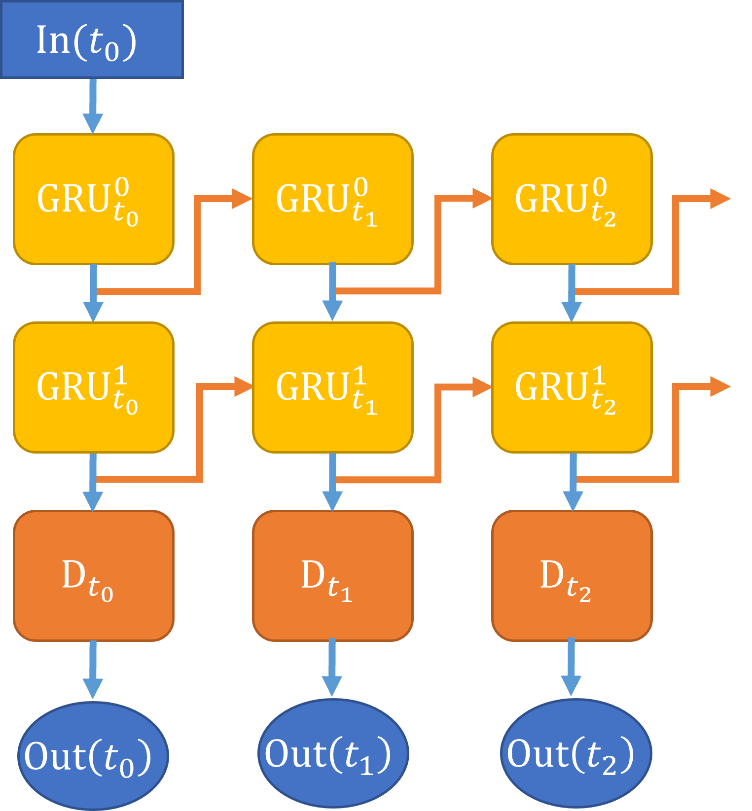
(a)

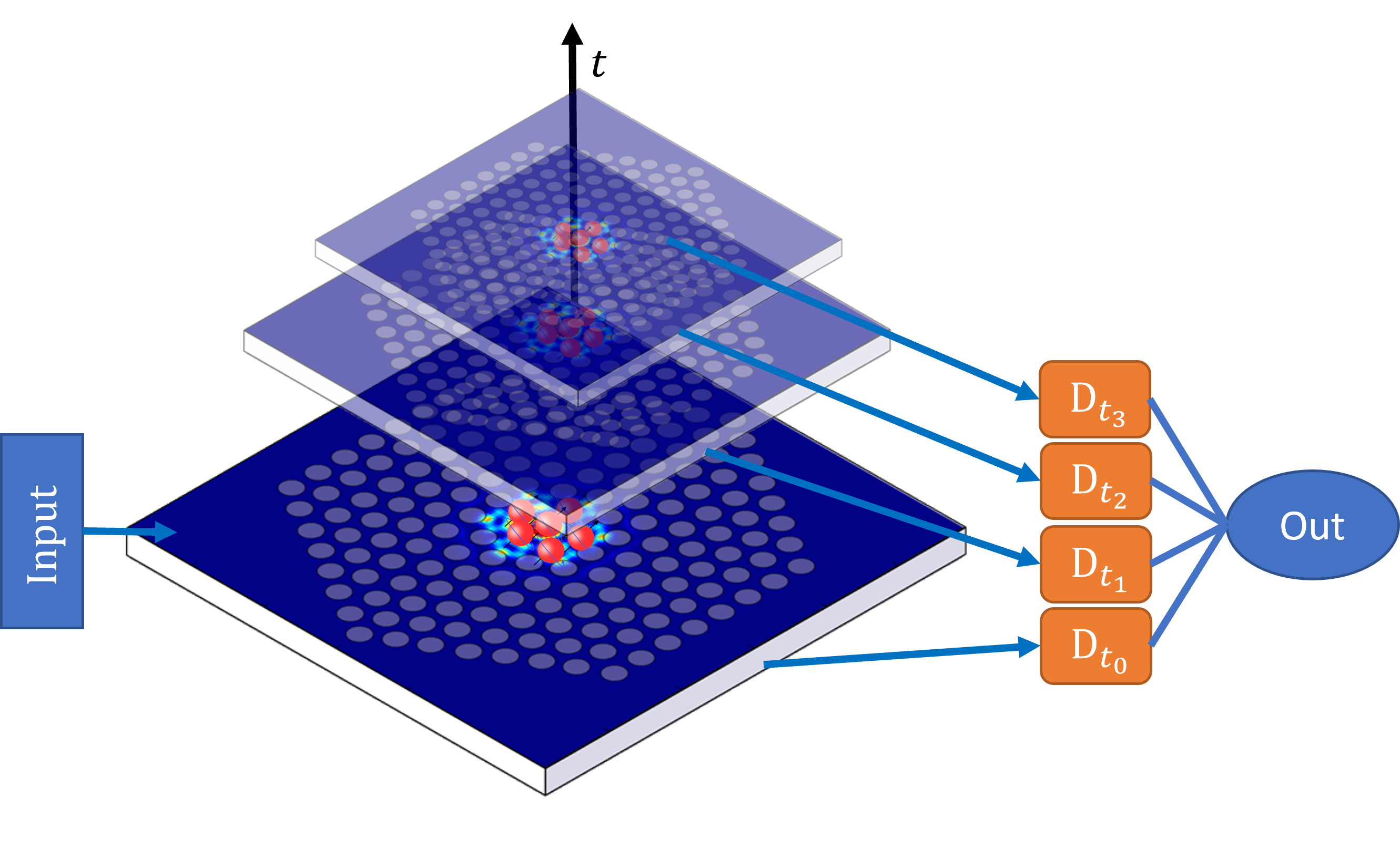
(b)

Figure 1: (a) Schematic of a recurrent neural network, showing the input to the output pathways including GRU layers [9] (a type of RNN layer) . Information is passed vertically through layers (blue arrows) and horizontally (orange arrows) between GRU timesteps to embed memory of previous timesteps. In such an RNN, many internal weights of the GRU layer need to be updated by back-propagation, making it an effective but computationally expensive architecture. (b) Schematic of the Quantum Physical Reservoir Computing network, an input is fed into the open quantum system and the time series of the quantum state evolution is fed into the dense layer at the end of the network. In this case, only the dense layer weights are updated.

II Quantum Physical Reservoir System

A prerequisite of an effective physical reservoir computer is that the reservoir behaves predictably and produces the same output for a given input. A dissipative system, such as an atomic system embedded in a lossy cavity, will tend towards an equilibrium state if the system’s evolution is well controlled. Then by reducing the temperature, this equilibrium state will roughly coincide with the ground state of the atomic systems and the local reservoir. Laser drives can be used to generate effective initial conditions from a given input data set, ensuring that the system acts predictably[13, 30, 37]. In order to effectively deploy our QPRC approach, we need to identify a large open quantum system model that can be sampled effectively. The model system we are focusing on is many-body atomic systems placed inside of a single lossy photonic cavity [6]. The dynamics of the composite system is governed by the Hamiltonian:

$$H= \sum_{i=1}^{N}\omega_{0}\sigma_{i}^{+}\sigma_{i}^{-}+\sum_{\lambda}\omega_{\lambda}a^{\dagger}_{\lambda}a_{\lambda}+$$

$$i\sum_{i,\lambda}g_{\lambda}(a_{\lambda}\sigma^{+}_{i}-a^{\dagger}_{\lambda}\sigma^{-}_{i})+\sum_{i\neq j}\Lambda\sigma^{+}_{i}\sigma_{j}^{-}.$$ (1)

where $\sigma_{i}^{+}$and $\sigma_{i}^{-}$ are the excitation and de-excitation operators for the $i^{\textrm{th}}$ atomic system respectively, $a_{\lambda}$ and $a^{\dagger}_{\lambda}$ are the bosonic field annihilation and creation operators, $\omega_{0}$ and $\omega_{\lambda}$ are the atomic transition and the $\lambda$-boson mode frequencies, $g_{\lambda}$ is the coupling strength of the atomic system and the $\lambda$-boson mode and $\Lambda$ is the dipole-dipole coupling strength between atoms [35, 43, 22]. This is equivalent to a Dicke model [12] for $N$-atoms with an inter-atom coupling. We have chosen a highly symmetric atomic system to generate time-resolved data efficiently. To this extent, we also limit our investigation to the single-excitation regime. We also assume an initial condition given by

$$\phi(0)=c_{0}\psi_{0}+\sum_{i}^{N}c_{i}(0)\psi_{i}+\sum_{\lambda}c_{\lambda}(0)\psi_{\lambda},$$ (2)

where $\psi_{i}=\ket{i}_{A}\ket{0}_{B}$ is the state wherein the $i^{\textrm{th}}$atom is in its excited state and all other atoms and the photonic cavity are in the ground state. $\psi_{\lambda}=\ket{0}_{A}\ket{\lambda}_{B}$ represents all atoms in their ground state, and the cavity system has its $\lambda$ mode excited. $\psi_{0}=\ket{0}_{A}\ket{0}_{B}$ denotes the ground state of the entire system.

Then the time evolution of this initial state is given by

$$\phi(t)=c_{0}\psi_{0}+\sum_{i}^{N}c_{i}(t)\psi_{i}+\sum_{\lambda}c_{\lambda}(t)\psi_{\lambda}.$$ (3)

Using an adiabatic cancellation of the photonic mode variables $c_{\lambda}$ and introducing the memory kernel

$$G(t)=\sum_{\lambda}g_{\lambda}^{2}e^{i(\omega_{0}-\omega_{\lambda})t},$$ (4)

the equations of motion for the atomic degrees of freedom can be expressed as

$$\dot{c}_{i}= -i\Lambda(c_{+}-c_{i})-\int^{t}_{0}G(t-t_{1})c_{+}(t_{1})dt_{1},$$ (5)

where $c_{+}=\sum_{i}^{N}c_{i}$. The non-Markovian or memory effects in the system’s dynamics are associated with this convolution over the memory kernel at previous times. This is precisely the aspect of our QPRC implementation that we intend to leverage.

The time evolution of this system is then determined by the distribution of the coupling strengths given by the spectral density

$$J(\omega)=\sum g_{\lambda}^{2}\delta(\omega-\omega_{\lambda}),$$ (6)

which is related to the memory kernel by the simple relation

$$G(t)=\int d\omega J(\omega)e^{i(\omega_{0}-\omega)t}.$$ (7)

For a lossy photonic cavity on-resonance with the atomic transitions, it is common to model the spectral density by a Lorentzian distribution of the form

$$J(\omega)=\frac{\lambda\gamma}{\gamma^{2}+(\omega-\omega_{0})^{2}}.$$ (8)

$\lambda$ is the coupling strength of the atoms to the cavity mode, and $\gamma$ determines the spectral width of the lossy cavity [28, 2, 26].

As a result, the time evolution of the excited state amplitudes for the $i^{\textrm{th}}$atom is given by

$$c_{i}(t) =(c_{i}(0)-\frac{c_{+}(0)}{N})e^{i\Lambda t}$$

$$+\frac{c_{+}(0)}{N}e^{-\mu^{*}t}\left(\cosh(\Gamma t)+\frac{\mu}{\Gamma}\sinh(\Gamma t)\right),$$ (9)

where we have introduced the following for convenience the following notations

$$\Lambda_{FC} =J(N-1)$$

$$\Gamma =\frac{1}{2}\sqrt{\gamma^{2}-2i\gamma\Lambda_{FC}-\Lambda_{FC}^{2}-4\lambda N}$$

$$\mu =\frac{1}{2}\big{(}\gamma-i\Lambda_{FC}\big{)}.$$ (10)

In order to utilize this physical system as a QPRC layer, we require a procedure for inputting data into the QPRC layer and subsequently outputting it into the neural network. For a stream of input data given by $\mathcal{I}$, we need to define a bijection $f$ that maps $\mathcal{I}$ to the multi-valued ensemble of values $c=\{c_{i}\}$. Then we require an map $g$ that transfers $\phi(t)$ to $\mathcal{O}$, the output of the QPRC layer, which is then passed directly into the conventional neural network layers. The particular map $g$ we utilize in the following is the real and imaginary components of the excited state amplitudes at various timesteps $\{t_{j}\}$, $g:\phi(t)\rightarrow\{\Re{c_{i}(t_{j})},\Im{c_{i}(t_{j})}\}$ akin to performing non-demolition measurements on the system or quantum state tomography[10, 16] .

III Quantum Physical Reservoir for Image Recognition

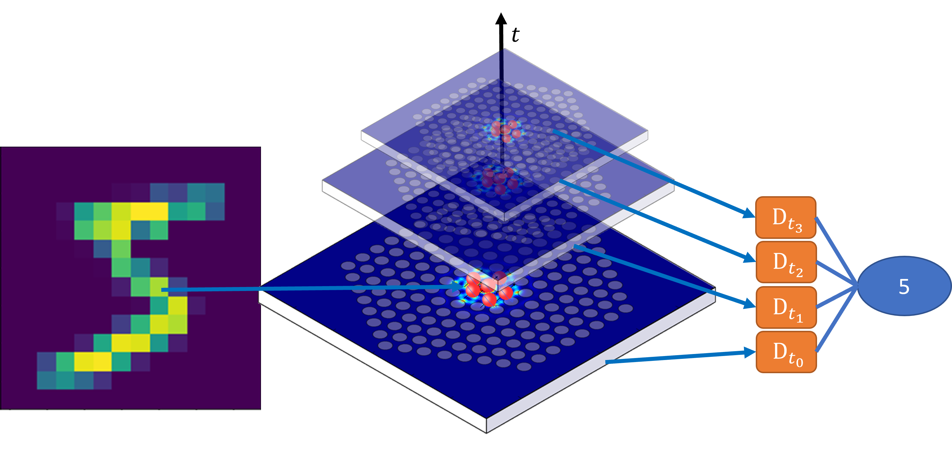
(a)

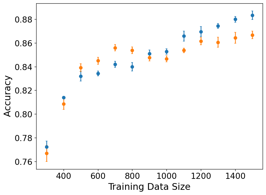
(b)

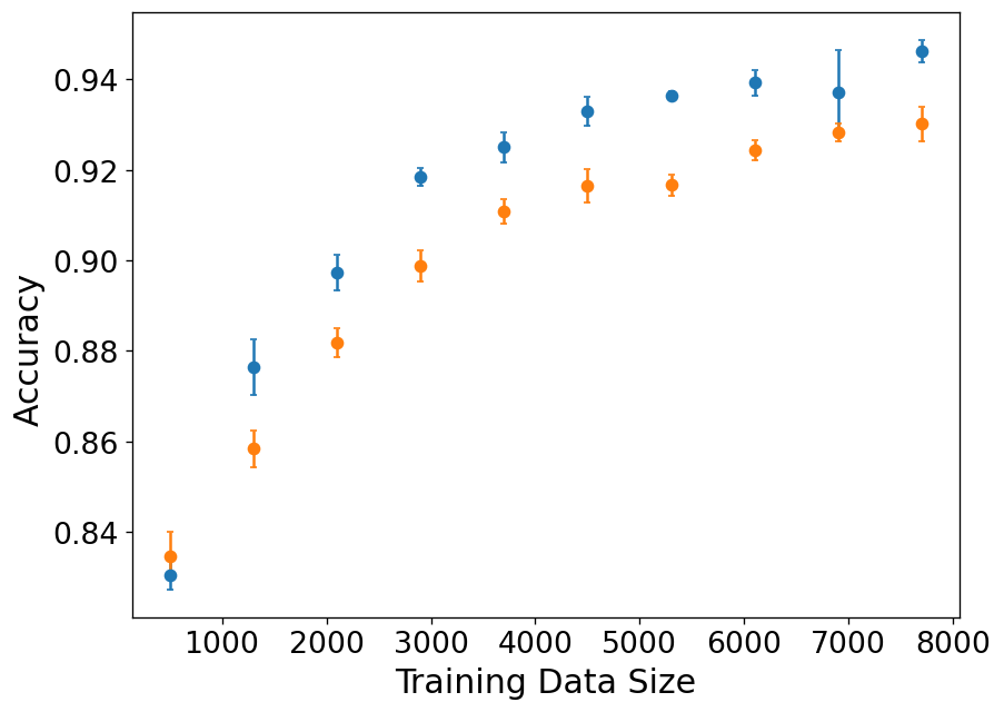
(c)

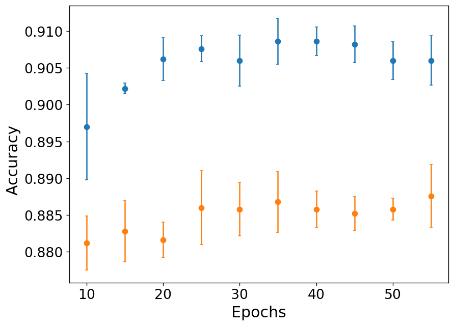
(d)

Figure 2: (a) Schematic of the Quantum Physical Reservoir network used to implement image recognition; pixel data is converted into an initial condition for the open quantum system, and the time series of the quantum state is fed into the dense layer at the end of the network. Only dense layer weights are updated. (b-d) The accuracy, as a fraction of correct predictions, of the QPRC approach (blue) and the conventional neural network without the QPRC layer (orange) for (b,c) varying sizes of training data (c) varying numbers of training epochs.

Having defined the dynamical process of our QPRC framework, we deploy it to solve an archetypal problem in machine learning, and pattern recognition using the standard MNIST database[11]. The MNIST database is a collection of monochrome images of handwritten numbers from 0-9 and the task is to classify what number each image represents successfully. In order to effectively deploy our reservoir computing approach, we need to identify an isometry between the pixel data for each image and an initial condition for the state of our system. To this end, we use the pixel brightness of the $2n$ and $2n+1$ pixel and map it directly to the real and imaginary component of $c_{n}(0)$ and then normalize the wavefunction $\phi(0)$.

Mathematically, for an image with $i^{\textrm{th}}$pixel brightness given by $P_{i}$ we have the mapping $c_{i}=(P_{i}+iP_{i+1})/\mathcal{N}$, where $\mathcal{N}$ is a normalisation constant. Then the wavefunction is time-evolved (see per Eqn. 9) and sampled at $n=50$ equal time steps up to $n\cdot\omega_{0}^{-1}$. The time series’ real and imaginary components are then passed into a reduced neural network. The reduced neural network consists of a single dense layer of dimension $n_{\textrm{nn}}=128$. A pictorial schematic of this procedure is given in Fig.2(a). The elegance of this approach is that we need only perform the gradient descent on the small final dense layer of the network, reducing the most complex step of readjusting network weights. With this procedure developed, we performed two numerical experiments. First, how does the QPRC network compare to a neural network without the QPRC layer for varying sizes of training data? The results of this experiment are presented in Fig. 2(b) and (c). The QPRC neural network outperforms the conventional neural network for intermediate and large values of the training data, a regime in which we approach $>90\%$ accuracy in our prediction capabilities. Furthermore, we can identify a crossover point at which the QPRC begins to outperform the standard neural network at around 900 training sets. This suggests that the QPRC approach may outperform conventional approaches for large data sets. This is a remarkable result since. With the ever-increasing relevance of big-data and the massively growing nature of computational costs associated with extremely large neural networks used in natural language processing systems, it becomes more and more necessary to be find more efficient ways to handle large data sets. Furthermore, our results suggest that the QPRC neural network generates a more effective representation of the data set being studied. To demonstrate this, we compared the QPRC network performance against a conventional neural network for varying numbers of training epochs. The results presented in Fig.2(d) clearly show that the QPRC system outperforms the non-QPRC network at all values of the training epoch sampled. All numerical experiments shown in Fig. 2 have been repeated five times at each sampling point, and the errors on the graph are the standard deviations from these five samples. In the experiments, we used a single dense layer of dimension 128, with a $\tanh$ activation function; the Adam optimizer was used with a learning rate of 0.001 and 30 training epochs.

The QPRC platform introduced here can further be optimized to increase its performance and accuracy. Here we could exploit the correlations in the data set to guide the QPRC system choice. Due to pixel data displaying strong nearest-neighbour correlations, a nearest neighbour type of interaction in the quantum system would increase the approach’s efficacy. Such a system may consist of a 2D lattice of atomic systems embedded in an array of photonic cavities with controllable cavity-cavity positioning. This architecture, this 2D lattice geometry, would lead to a nearest neighbour interaction between the atomic systems and thus generate commensurate nearest neighbour correlations to the pixel data.

IV Quantum Physical Reservoir Computing Approach for Open Quantum Systems

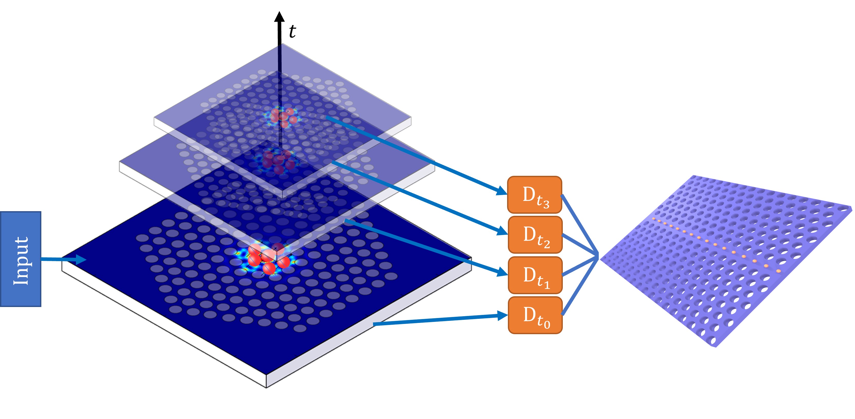
(a)

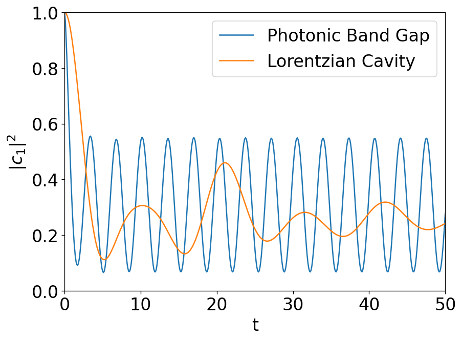
(b)

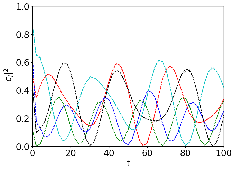
(c)

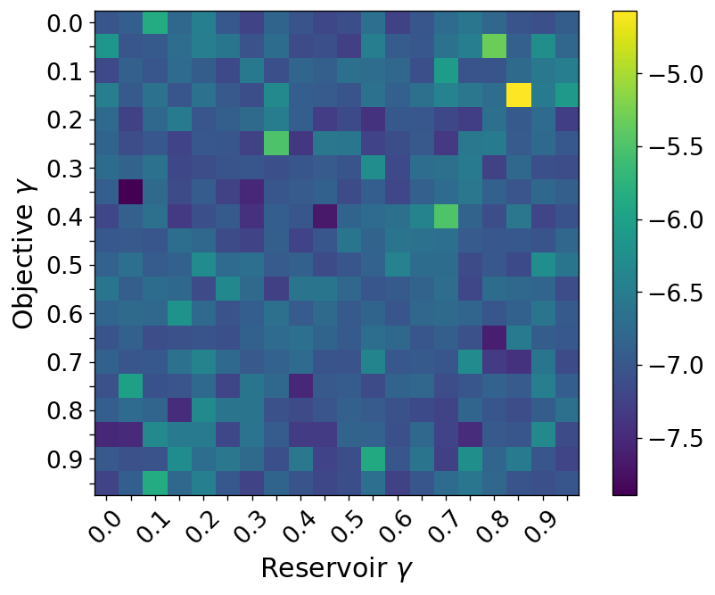
(d)

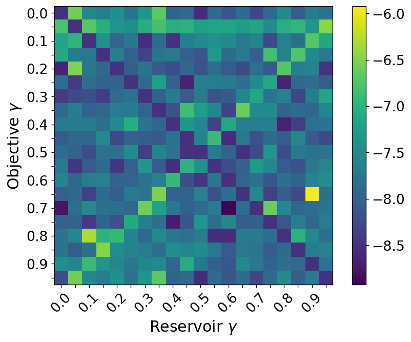
(e)

Figure 3: (a) Schematic of the Quantum Physical Reservoir network used to predict the dynamics of atoms embedded in a photonic band gap material. (b) Population dynamics of a single atom coupled to another atom inside of a photonic crystal and inside of a photonic cavity. The photonic crystal allows for non-zero steady state populations due to strong coupling to the band edge mode. (c) The prediction of the QPRC approach (dotted) and the real dynamics (dashed) of two coupled atoms inside of a photonic band gap material for randomly sampled initial conditions. (d,e) Heatmap to show the average error of the QPRC for varying values of both the reservoir and objective system’s spectral width $\gamma$. The heatmap depicts average $\log_{10}$ of the errors for QPRCs for two simulated run times (d) $10\omega_{0}^{-1}$ (e) $100\omega_{0}^{-1}$.

In the previous section, we demonstrated the QPRC approach’s usefulness in enhancing conventional neural networks’ performance in pattern recognition tasks. Here, we focus on extending this approach to deal with quantum mechanical problems. Specifically, we study the efficacy of the QPRC approach in understanding the dynamics of open quantum systems schematically presented in Fig. 3(a). It is often impossible to describe the dynamics of the combined quantum system of interest and environment in open quantum systems. Various approximations are deployed to model the influence of the environment’s degrees of freedom on the system of interest evolution. However, these approximations also have some limitations. A standard approximation in the field is the Markov approximation; wherein there is a unidirectional dissipation of information from the system into the environment. This approximation is only valid when the environment relaxes on timescales much faster than the systems such that the system barely perturbs the environment, akin to a weak coupling limit assumption.

This method has been successful in analyzing many systems, however it falls short in capturing quantum-induced memory effects. For instance, in highly structure photonic systems, such as photonic crystals, the local density of states for the electromagnetic field undergo rapid fluctuation quickly for frequencies close to the band edges of the photonic band gap. When a two-level atomic system is embedded with its transition energy close to the band edge of a photonic bandgap, the Markov approximation is rendered invalid due to the strong fluctuations [5, 15, 20], and extremely non-Markovian dynamics emerge. As a result of the strong interaction between the atomic system and the photonic reservoir, the atomic states become highly intertwined with the properties of the photonic reservoir and the degrees of freedom of the atoms. This results in temporal oscillations, fractional atomic population decay, spectral splitting, and sub-natural line-widths of atomic transitions [21].

Furthermore, it has been demonstrated that the coherence lifetime of multi-qubit systems may be increased by effectively characterising the non-Markovian noise [42]. This emphasises the necessity of learning more about how many-bodied systems interact with non-Markovian environments. Understanding these control processes may help design and create more reliable and performant quantum technologies, including quantum clocks [24] and quantum networks [23]. Beyond the preservation of entanglement, another challenge faced by quantum technology is the creation of such entanglement. An intriguing recent discovery demonstrates that it is viable to use the environment’s non-Markovianity to create entanglement between atomic systems that were previously uncorrelated [31, 14].

Here we explore the efficacy of the lossy cavity atomic ensemble QPRC in capturing the dynamics of a strongly non-Markovian system, in which a two-level atomic ensemble coupled to a photonic reservoir associated with a photonic band gap material. We have used the isotropic one-dimensional photonic crystal band edge model for our photonic crystal. Such systems can be constructed using a photonic crystal waveguide. This fascinating system generates strong atom-photon coupling. This is due to a divergence in the local density of states of the electromagnetic field modes around the band edge frequency $\omega_{I}$ ($\rho(\omega)\propto(\omega-\omega_{I})^{-\frac{1}{2}}$). The Hamiltonian for this system is as in Eqn.1, leading to the convolution of states given by Eqn.5. However, due to the divergence in the density of states around the photonic band edge, the memory kernel takes the form

$$\tilde{G}(s)=\beta^{3/2}e^{-i\pi/4}(s-i(\omega-\omega_{I}))^{-\frac{1}{2}},$$ (11)

where $\beta$ is the coupling strength. This divergence in the memory kernel leads to strong non-Markovian effects in the system generating a plethora of new features such as fractional decay of the atomic systems and photon-atom bound states [21, 20, 15]. In Fig. 3(c), we present the dynamics of a coupled pair of atoms inside a Lorentzian cavity and a photonic band gap material. We note that these two systems undergo very different dynamics. In the single atom case, the lossy cavity will dissipate all of the energy in the excited state at the steady state. In contrast, the atom placed inside the photonic band gap materials displays strongly non-Markovian dynamics. Due to the splitting of the energetic states by strong coupling to the lower photonic band edge some of the excitation is maintained even to the steady state giving rise to the fractional decay. Next, we train the QPRC network to model the non-Markovian dynamics of the atoms in the photonic band gap system. To achieve this, we initialised our QPRC system with the same initial conditions as the photonic band gap system we wanted to model. That is, our input $c(0)$ is the same for both the QPRC and the photonic band gap system. The output of the QPRC is then fed into a small neural network of 3 dense layers, which are subsequently updated via standard back-propagation. The results presented in Fig. 3(b) demonstrate the ability of two-atom QPRC to predict the dynamics of two atoms bound within the photonic band gap. Even for a relatively small sample size of 1500 data-sets and despite the distinctive dynamics of the two systems, the QPRC framework is very accurate in predicting the complex dynamics of the system. Next, we tested the efficacy of cavities of different spectral widths against one another; here we have the same setup as in the previous experiment. To test multiple configurations of the cavity systems, we varied the spectral width $\gamma$ of both the QPRC system and the target system we wanted to model. The results shown in Figs.3(d) and (e) demonstrate that the QPRC system is highly effective at capturing the dynamics of similar systems, showing average errors of $10^{-7}$ across the data sets.

Furthermore, we extended the run time of the reservoir from $10\omega_{0}^{-1}$ to $100\omega_{0}^{-1}$ (see Fig. 3(d)), and remarkably we find that efficacy of the reservoir increases greatly now with average errors in the range of $10^{-8}$. The QPRC approach is not only simply maintaining a representation of the input state but is performing useful computation due to the expansion of the input into a higher dimensional computational space brought about by its intricate non-Markovian dynamics.

V Conclusion

In summary, we have introduced a QPRC system consisting of two-level atomic systems coupled to Lorentzian photonic cavities as a model open quantum system. We have applied the QPRC approach to a classic machine learning challenge of recognizing images from the MNIST database. The efficacy of the QPRC was compared to a neural network with the same design but without a QPRC layer. Remarkably, our results revealed that the QPRC is underperforming against the traditional neural network for relatively small training data sets but rapidly starts to outperform it for larger data set sizes. This result has significant implications since modern neural networks are quickly bottlenecked by the size of the data they can effectively model. Furthermore, we used a fixed data set size to assess the efficacy versus the number of training epochs and demonstrated that the QPRC outperformed the traditional neural network approach at each epoch number examined. Finally, we have demonstrated the efficiency of the QPRC approach in modelling the dynamics of atomic systems coupled to cavities of various quality, atomic systems in photonic band gap materials, and open quantum systems challenges. The QPRC was very efficient in producing accurate representations of capturing the complexities of the quantum dynamics of these systems, even with a small amount of training data. The physical platform introduced here for QPRC paves the way for a new approach to scalable quantum machine learning, vastly outperforming conventional recurrent neural network approaches.

- [1] L. Banchi, E. Grant, A. Rocchetto, and S. Severini. Modelling non-markovian quantum processes with recurrent neural networks. New Journal of Physics, 20(12):123030, dec 2018.
- [2] S. M. Barnett and J. Jeffers. The damped jaynes–cummings model. Journal of Modern Optics, 54(13-15):2033–2048, 2007.
- [3] R. A. Bravo, K. Najafi, X. Gao, and S. F. Yelin. Quantum reservoir computing using arrays of rydberg atoms. PRX Quantum, 3:030325, Aug 2022.
- [4] H. P. Breuer and F. Petruccione. The theory of open quantum systems. Oxford University Press, Great Clarendon Street, 2002.
- [5] A. Burgess and M. Florescu. Modelling non-Markovian dynamics in photonic crystals with recurrent neural networks. Opt. Mat. Express, 11(7):2037, July 2021.
- [6] A. Burgess and M. Florescu. Non-markovian dynamics of a single excitation within many-body dissipative systems. Phys. Rev. A, 105:062207, Jun 2022.
- [7] G. Carleo and M. Troyer. Solving the quantum many-body problem with artificial neural networks. Science, 355(6325):602–606, 2017.
- [8] D. E. Chang, V. Vuletić, and M. D. Lukin. Quantum nonlinear optics — photon by photon. Nature Photonics, 8(9):685–694, Sep 2014.
- [9] J. Chung, Ç. Gülçehre, K. Cho, and Y. Bengio. Empirical evaluation of gated recurrent neural networks on sequence modeling. CoRR, abs/1412.3555, 2014.
- [10] M. Cramer, M. B. Plenio, S. T. Flammia, R. Somma, D. Gross, S. D. Bartlett, O. Landon-Cardinal, D. Poulin, and Y.-K. Liu. Efficient quantum state tomography. Nature Communications, 1(1):149, Dec 2010.
- [11] L. Deng. The mnist database of handwritten digit images for machine learning research. IEEE Signal Processing Magazine, 29(6):141–142, 2012.
- [12] R. H. Dicke. Coherence in spontaneous radiation processes. Phys. Rev., 93:99–110, Jan 1954.
- [13] C. Dory, K. A. Fischer, K. Müller, K. G. Lagoudakis, T. Sarmiento, A. Rundquist, J. L. Zhang, Y. Kelaita, and J. Vučković. Complete coherent control of a quantum dot strongly coupled to a nanocavity. Scientific Reports, 6(1):25172, Apr 2016.
- [14] C. H. Fleming, N. I. Cummings, C. Anastopoulos, and B. L. Hu. Non-markovian dynamics and entanglement of two-level atoms in a common field. Journal of Physics A: Mathematical and Theoretical, 45(6):065301, jan 2012.
- [15] M. Florescu and S. John. Single-atom switching in photonic crystals. Phys. Rev. A, 64:033801, Aug 2001.
- [16] P. Grangier, J. A. Levenson, and J.-P. Poizat. Quantum non-demolition measurements in optics. Nature, 396(6711):537–542, Dec 1998.
- [17] J. Hirschberg and C. D. Manning. Advances in natural language processing. Science, 349(6245):261–266, 2015.
- [18] H.-Y. Huang, M. Broughton, J. Cotler, S. Chen, J. Li, M. Mohseni, H. Neven, R. Babbush, R. Kueng, J. Preskill, and J. R. McClean. Quantum advantage in learning from experiments. Science, 376(6598):1182–1186, 2022.
- [19] H.-Y. Huang, R. Kueng, G. Torlai, V. V. Albert, and J. Preskill. Provably efficient machine learning for quantum many-body problems. Science, 377(6613):eabk3333, 2022.
- [20] S. John and M. Florescu. Photonic bandgap materials: towards an all-optical micro-transistor. Journal of Optics A: Pure and Applied Optics, 3(6), 2001.
- [21] S. John and T. Quang. Spontaneous emission near the edge of a photonic band gap. Physical Review A, 50(2):1764–1769, Aug. 1994.
- [22] S. John and T. Quang. Localization of superradiance near a photonic band gap. Phys. Rev. Lett., 74:3419–3422, Apr 1995.
- [23] H. J. Kimble. The quantum internet. Nature, 453(7198):1023–1030, Jun 2008.
- [24] P. Kómár, E. M. Kessler, M. Bishof, L. Jiang, A. S. Sørensen, J. Ye, and M. D. Lukin. A quantum network of clocks. Nature Physics, 10(8):582–587, Aug 2014.
- [25] M. Krenn, M. Malik, R. Fickler, R. Lapkiewicz, and A. Zeilinger. Automated search for new quantum experiments. Phys. Rev. Lett., 116:090405, Mar 2016.
- [26] G. Kurizki, A. G. Kofman, A. Kozhekin, and G. Harel. Control of atomic state decay in cavities and microspheres. New Journal of Physics, 2(1):328, dec 2000.
- [27] R. Kuszelewicz, J.-M. Benoit, S. Barbay, A. Lemaître, G. Patriarche, K. Meunier, A. Tierno, and T. Ackemann. High density inalas/gaalas quantum dots for non-linear optics in microcavities. Journal of Applied Physics, 111(4):043107, 2012.
- [28] J.-G. Li, J. Zou, and B. Shao. Non-markovianity of the damped jaynes-cummings model with detuning. Phys. Rev. A, 81:062124, Jun 2010.
- [29] M. Lukoševičius and H. Jaeger. Reservoir computing approaches to recurrent neural network training. Computer Science Review, 3(3):127–149, 2009.
- [30] J. Miguel-Sánchez, A. Reinhard, E. Togan, T. Volz, A. Imamoglu, B. Besga, J. Reichel, and J. Estève. Cavity quantum electrodynamics with charge-controlled quantum dots coupled to a fiber fabry–perot cavity. New Journal of Physics, 15(4):045002, apr 2013.
- [31] N. Mirkin, P. Poggi, and D. Wisniacki. Information backflow as a resource for entanglement. Phys. Rev. A, 99:062327, Jun 2019.
- [32] K. Nakajima. Physical reservoir computing—an introductory perspective. Japanese Journal of Applied Physics, 59(6):060501, may 2020.
- [33] D. Patterson, J. Gonzalez, Q. Le, C. Liang, L.-M. Munguia, D. Rothchild, D. So, M. Texier, and J. Dean. Carbon emissions and large neural network training, 2021.
- [34] D. Pfau, J. S. Spencer, A. G. D. G. Matthews, and W. M. C. Foulkes. Ab initio solution of the many-electron schrödinger equation with deep neural networks. Phys. Rev. Research, 2:033429, Sep 2020.
- [35] P. Pfeifer. Radiative decay versus photonic jahn-teller distortion of molecular states. Phys. Rev. A, 26:701–704, Jul 1982.
- [36] M. S. Rudolph, N. B. Toussaint, A. Katabarwa, S. Johri, B. Peropadre, and A. Perdomo-Ortiz. Generation of high-resolution handwritten digits with an ion-trap quantum computer. Phys. Rev. X, 12:031010, Jul 2022.
- [37] J. Schall, M. Deconinck, N. Bart, M. Florian, M. von Helversen, C. Dangel, R. Schmidt, L. Bremer, F. Bopp, I. Hüllen, C. Gies, D. Reuter, A. D. Wieck, S. Rodt, J. J. Finley, F. Jahnke, A. Ludwig, and S. Reitzenstein. Bright electrically controllable quantum-dot-molecule devices fabricated by in situ electron-beam lithography. Advanced Quantum Technologies, 4(6):2100002, 2021.
- [38] D. Silver, A. Huang, C. J. Maddison, A. Guez, L. Sifre, G. van den Driessche, J. Schrittwieser, I. Antonoglou, V. Panneershelvam, M. Lanctot, S. Dieleman, D. Grewe, J. Nham, N. Kalchbrenner, I. Sutskever, T. Lillicrap, M. Leach, K. Kavukcuoglu, T. Graepel, and D. Hassabis. Mastering the game of go with deep neural networks and tree search. Nature, 529(7587):484–489, Jan 2016.
- [39] G. Tanaka, T. Yamane, J. B. Héroux, R. Nakane, N. Kanazawa, S. Takeda, H. Numata, D. Nakano, and A. Hirose. Recent advances in physical reservoir computing: A review. Neural Networks, 115:100–123, 2019.
- [40] J. Tuszyński and J. Dixon. Non-linearity and the emergence of coherence in strongly interacting many-body systems near a critical point. Physics Letters A, 140(4):179–184, 1989.
- [41] S. Wakabayashi, T. Arie, S. Akita, K. Nakajima, and K. Takei. A multitasking flexible sensor via reservoir computing. Advanced Materials, 34(26):2201663, 2022.
- [42] G. A. L. White, C. D. Hill, F. A. Pollock, L. C. L. Hollenberg, and K. Modi. Demonstration of non-markovian process characterisation and control on a quantum processor. Nature Communications, 11(1):6301, Dec 2020.
- [43] S. Zienau. Optical resonance and two level atoms. Physics Bulletin, 26(12):545–546, dec 1975.