Robust nonparametric regression: review and practical considerations.

Abstract

Nonparametric regression models offer a way to understand and quantify relationships between variables without having to identify an appropriate family of possible regression functions. Although many estimation methods for these models have been proposed in the literature, most of them can be highly sensitive to the presence of a small proportion of atypical observations in the training set. A review of outlier robust estimation methods for nonparametric regression models is provided, paying particular attention to practical considerations. Since outliers can also influence negatively the regression estimator by affecting the selection of bandwidths or smoothing parameters, a discussion of robust alternatives for this task is also included. Using many of the “classical” nonparametric regression estimators (and their robust counterparts) can be very challenging in settings with a moderate or large number of explanatory variables, so recently proposed robust nonparametric regression methods that scale well with a growing number of covariates are also discussed.

1 Introduction

Regression models can be used to either understand and quantify the relationship between a certain variable $Y\in\mathbb{R}$ (generally called the “response”) and a number of “explanatory” ones (or “features”) ${\mathbf{X}}$, or to construct predictions for $Y$ based on future values of ${\mathbf{X}}$. Note that typically ${\mathbf{X}}\in\mathbb{R}^{d}$, $d\in\mathbb{N}$, but some models and estimation methods can be extended naturally to more general cases where ${\mathbf{X}}\in{\cal X}$, a metric space (e.g. ${\mathbf{X}}$ could be an image or a smooth function). In what follows we will consider a general regression model of the form

$$Y=f({\mathbf{X}})+\varepsilon\,,$$ (1)

where $f$ is a real valued unknown function, and $\varepsilon$ is a random variable that models random fluctuations not accounted by $f$. Furthermore, we will be concerned with the possible presence of atypical observations or with heavy-tailed error distributions. Thus, we will avoid requiring that moments of $\varepsilon$ necessarily exist, and instead assume that the conditional distribution function of $\varepsilon$ given ${\mathbf{X}}$ is of the form

$$F_{\varepsilon|{\mathbf{X}}}(u)=F_{0}(u/\sigma_{{\mathbf{X}}})\,,$$ (2)

for a fixed distribution function $F_{0}$ that is symmetric around zero, and where $\sigma_{{\mathbf{X}}}>0$ is the error scale parameter, which is typically unknown. Note that (2) is a particular case of a more general formulation that would specify $F_{\varepsilon|{\mathbf{X}}}(u)=F_{0}(u,{\mathbf{X}})$. The setting on which we focus implies that any heteroskedasticity in the data is due to a changing dispersion coefficient (e.g. standard deviation, if second moments exist), rather than more general changes in the shape or family of the error distribution, for example. Although the particular functional form of the dependence of the distribution of $\varepsilon$ conditional on ${\mathbf{X}}$ is not critical, we will see below that to be able to use robust estimators for these models, the mechanism of this dependence will need to be assumed explicitly, in order for the residuals in the estimating equations to be adjusted appropriately.

A widely used class of regression models assumes that the regression function $f$ in (1) belongs to a family parametrized by a finite dimensional vector: ${\cal F}=\left\{f_{\mathbf{\theta}},\,{\mathbf{\theta}}\in\Theta\subseteq\mathbb{R}^{k}\right\}$. In this case, the problem of estimating $f$ reduces to that of estimating the vector ${\mathbf{\theta}}$. A clear limitation of adopting this framework is that, to avoid drawing biased conclusions due to model misspecification, the family ${\cal F}$ needs to be rich enough to include the unknown $f$ in (1). Although in some applications subject matter knowledge (e.g. physical models) may prescribe an appropriate family ${\cal F}$, there are many practical situations where no obvious parametric model exists and a different approach is necessary.

Nonparametric regression analysis refers to the collection of estimation methods for $f$ that do not assume a finite dimensional parametric model for it. Nonparametric methods can coarsely be classified into two groups, which we will call “unstructured” and “semi-structured”, respectively. “Unstructured” approaches place almost no asumption or restriction on the shape or structure of the regression function or its estimator. An example is given by local (kernel) regression methods. “Semi-structured” approaches, on the other hand, impose some structure on $f$, or, more often, on its estimator $\hat{f}$. Examples in this latter class include additive models, and regression trees. These constraints generally result in estimators that may be notably less variable than “unstructured” ones, and thus have lower prediction errors if the bias induced by the added structure is sufficiently small. This coarse taxonomy of non-parametric regression estimators is not meant to be exhaustive, and there are methods and models that do not fall clearly in either of these two groups. However, we believe that it is useful to organize our discussion below.

There are also some models that are neither fully parametric nor completely nonparametric. These are often called semiparametric in the literature. One popular class of such models are index models, where ${\mathbf{X}}\in\mathbb{R}^{d}$ with $d>1$, and the regression function is assumed to satisfy

$$f({\mathbf{X}})=\mu+\sum_{j=1}^{p}f_{j}({\mathbf{X}}^{\top}{\mathbf{\alpha}}_{j})\,,$$

where $\mu\in{\mathbb{R}}$, $f_{j}:{\mathbb{R}}\to{\mathbb{R}}$ are smooth functions of a single argument, and $\alpha_{j}\in{\mathbb{R}}^{d}$. Obvious ambiguity in the expression above can be avoided if one assumes that $f_{j}(0)=0$, $\|{\mathbf{\alpha}}_{j}\|_{2}=1$, and that the first non-zero element of ${\mathbf{\alpha}}_{j}$ is positive, for all $1\leq j\leq p$. However, identifiability of these models is a delicate problem (Horowitz, 1998, page 14). We refer the interested reader to Yuan (2011) and references therein. Robust estimators for these models proposed in the literature focus on estimating the projections ${\mathbf{\alpha}}_{j}$. Another class of semiparametric models is that of partly linear models where $f$ is assumed to depend linearly on some covariates and also include a non-parametric component:

$$f({\mathbf{X}},u)={\mathbf{\beta}}^{\top}{\mathbf{X}}+g(u)\,,$$

where ${\mathbf{\beta}}\in{\mathbb{R}}^{d}$ and $g:{\mathbb{R}}\to{\mathbb{R}}$ is a smooth function. Robust estimators for these models are typically obtained by combining robust linear regression estimators with some of the nonparametric approaches discussed below.

Historically, the focus in the Statistics literature when it comes to regression problems has been on estimating the function $f$. Different approaches are generally compared with each other based on measures of uncertainty associated with the estimated values of $f$ at specific points of its domain, for example the mean squared error at ${\mathbf{x}}_{0}$:

$$E\left[(f({\mathbf{x}}_{0})-\hat{f}({\mathbf{x}}_{0}))^{2}\right]\,,$$ (3)

or with overal error measures such as the integrated squared error (ISE)

$$\mbox{ISE}=\int(f({\mathbf{x}})-\hat{f}({\mathbf{x}}))^{2}dF_{\mathbf{X}}({\mathbf{x}})\,,$$ (4)

where $F_{\mathbf{X}}$ denotes the distribution function of the explanatory variable ${\mathbf{X}}$. In recent decades many methods have been proposed to construct “predictors” for the response variable $Y$ at given values of ${\mathbf{X}}$ while remaining relatively agnostic about the regression function $f$ (e.g. random forests and gradient boosting). The main difference between estimation-based and prediction-based approaches lies in how one quantifies the “performance” of a specific method. Nevertheless, there is of course a natural connection between these two approaches: given an estimator $\hat{f}$ and a point ${\mathbf{x}}_{0}$, a natural prediction for $Y$ when ${\mathbf{X}}={\mathbf{x}}_{0}$ is $\hat{f}({\mathbf{x}}_{0})$. Similarly, one can estimate $f({\mathbf{x}}_{0})$ using a predictor by calculating the prediction $\hat{Y}$ for ${\mathbf{X}}={\mathbf{x}}_{0}$.

Estimators for the regression function $f$ are constructed using what is often called a “training set”. Namely, we assume that we have access to a data set ${\cal D}_{n}=\left\{(y_{i},{\mathbf{x}}_{i}),1\leq i\leq n\right\}$ that follows the model in (1). This assumption can be stated formally by considering a random object $(Y,{\mathbf{X}})$ where $Y=f({\mathbf{X}})+\varepsilon$ as in (1) and assuming that the points in ${\cal D}_{n}$ are a random sample from $(Y,{\mathbf{X}})$. The process of constructing $\hat{f}$ (an estimator, or a predictor) using ${\cal D}_{n}$ is called “estimation” in the traditional Statistics literature, and “learning” in the Machine Learning literature. In what follows we will use these terms exchangeably.

In the Statistics literature, nonparametric methods traditionally have been called “robust” in the sense of requiring fewer or weaker assumptions than their parametric counterparts to be consistent to the parameter or function of interest. However, these methods typically still require that the points in the training data are instances of the same random object (i.e. that every observation in ${\cal D}_{n}$ comes from the same population). In this paper we are concerned with methods that remain informative even when a proportion of the training sample may follow a different distribution. We will say that a method is “robust” when it is not unduly affected by a relatively small proportion of atypical observations in ${\cal D}_{n}$. It is well known that many non-parametric regression estimators and predictors are not robust in the latter sense. In other words, a few points in ${\cal D}_{n}$ that deviate from (1) may have a very large (even unbounded) effect on the estimator $\hat{f}$ or predictions $\hat{f}({\mathbf{x}}_{0})$. Robust methods are designed to avoid this problem while also maintaining a good performance when there are no “outliers” in the training set. The purpose of this paper is to review available robust alternatives for different non-parametric regression estimators.

We focus here on estimation and prediction methods to estimate the regression function $f$ as in (1) when the errors $\varepsilon$ have a symmetric distribution around zero. In this case, $f({\mathbf{x}}_{0})$ is the “center” of the conditional distribution of $Y$ given ${\mathbf{X}}={\mathbf{x}}_{0}$. In the interest of space, regression analysis methods with a different goal (e.g. quantile regression or modal regression) will not be included in this review.

Note that the infinite dimensional nature of the “parameter” space in nonparametric regression models limits the direct application of many of the standard robustness measures in the literature (e.g. breakdown point). There are few attempts in the literature to formalize and quantify the notion of robustness for these models. Tamine (2002) approached the problem in a point-wise manner, and derived smoothed influence functions for Nadaraya-Watson type estimators of $f(x)$ at each fixed point $x$. Giloni and Simonoff (2005) studied point-wise breakdown points of $L_{1}$ local polynomial regression estimators. Christmann and Steinwart (2007) and Steinwart and Christmann (2008, Section 10.4) studied the influence function of the function estimate $\hat{f}$ obtained using kernel-based regression (i.e. penalized regression over a reproducing kernel Hilbert space (RKHS) of functions with a bounded and continuous kernel). They found sufficient conditions for these influence functions to be bounded. Hable and Christmann (2011) and Christmann et al. (2013) showed that these RKHS estimators are also “stable” in the sense of being qualitatively robust (Hampel, 1971). Note that there is a natural “tension” between stability (qualitative robustness) and consistency, which intutitively is related to the richness of the “parameter space” (Hable and Christmann, 2013).

The rest of the paper is organized as follows. Sections 2 and 3 discuss “unstructured” and “semi structured” methods, respectively, along with their robust alternatives. Some reflections on the conceptual challenges of studying robustness in a non-parametric setting are included in Section 4.

2 Unstructured methods

Kernel-based estimation methods impose very weak structures on the estimated $f$’s. For example, although a local constant (Nadaraya-Watson) kernel estimator $\hat{f}(x_{0})$ is a linear function of the observed responses in the training set, the coefficients of the linear combination change non-linearly as functions of $x_{0}$, so the shape of $\hat{f}$ as a whole cannot be easily characterized. Penalized spline regression estimators (and regularized sieves (Grenander, 1981) estimators in general) are somewhat restricted (since $\hat{f}$ is a linear combination of the elements of the basis), but the spanned subspaces are usually quite complex and the dimensions of the bases increase with the training sample size, and thus it is not generally possible to describe explicitly the resulting family of estimators $\hat{f}$’s.

In this section we discuss both kernel and spline robust estimators for the regression function $f$ in (1), focusing on the case where both $Y$ and ${\mathbf{X}}$ are random objects. Robust fits based on local regression and splines methods can intuitively be constructed by simply replacing the squared loss function with one that either grows more slowly or is bounded. We show below that these arguably “ad hoc” approaches can in fact be justified formally from first principles.

2.1 Kernel-based methods

Under well known and relatively weak regularity conditions the regression function $f$ is the conditional expectation of $Y$ given ${\mathbf{X}}={\mathbf{x}}$:

$$f({\mathbf{x}})=E\left(Y|{\mathbf{X}}={\mathbf{x}}\right)\,.$$

This observation suggests that, given a sample ${\cal D}_{n}$, a “natural” estimator for $f({\mathbf{x}}_{0})$ is the Nadaraya-Watson local mean kernel estimator (Nadaraya, 1964; Watson, 1964). To fix ideas, consider first the case where ${\mathbf{X}}\in\mathbb{R}$, then

$$\hat{f}(x_{0})=\frac{\sum_{i=1}^{n}K_{h}(x_{i}-x_{0})\,y_{i}}{\sum_{j=1}^{n}K_{h}(x_{j}-x_{0})}\,,$$ (5)

where the weigths $K_{h}(x_{i}-x_{0})=(1/h)K((x_{i}-x_{0})/h)$ depend on a kernel function $K$, which is a non-negative and symmetric function that satisfies $\int K(u)du=1$, and the bandwidth $h>0$. For example, the Epanechnikov kernel is given by

$$K(u)=\frac{3}{4}\left(1-u^{2}\right)I(|u|\leq 1)\,,$$

where $I(A)$ is the indicator function of the set $A$. See Härdle et al. (2004) for more details. Note that $\hat{f}(x_{0})$ above satisfies

$$\hat{f}(x_{0})=\mathop{\rm argmin}_{a\in{\mathbb{R}}}\ \sum_{i=1}^{n}K_{h}\left(x_{i}-x_{0}\right)\,\left(Y_{i}-a\right)^{2}\,.$$ (6)

These estimators can be extended rather naturally to the case where ${\mathbf{X}}\in\mathbb{R}^{d}$ by using a multivariate kernel function $K_{H}$:

$$\hat{f}({\mathbf{x}}_{0})=\mathop{\rm argmin}_{a\in{\mathbb{R}}}\ \sum_{i=1}^{n}K_{{\mathbf{H}}}\left({\mathbf{x}}_{i}-{\mathbf{x}}_{0}\right)\,\left(Y_{i}-a\right)^{2}\,.$$ (7)

where often the matrix ${\mathbf{H}}=\text{diag}(h_{1},h_{2},\ldots,h_{d})$, with individual bandwidths, $h_{j}>0$, $K_{{\mathbf{H}}}({\mathbf{b}})={\cal K}_{d}({\mathbf{H}}^{-1}{\mathbf{b}})$, and the multivariate kernel ${\cal K}_{d}$ is the product of univariate kernels: ${\cal K}_{d}({\mathbf{b}})=\prod_{j=1}^{d}K(b_{j})$, for ${\mathbf{b}}=(b_{1},b_{2},\ldots,b_{d})^{\top}$, and $K$ is a univariate kernel as before. When the explanatory variables ${\mathbf{X}}$ are only assumed to take values in an arbitrary metric space ${\cal X}$ with distance $m(\cdot,\cdot)$, then the above estimator can be adapted in a natural manner, for example:

$$\hat{f}({\mathbf{x}}_{0})=\mathop{\rm argmin}_{a\in{\mathbb{R}}}\ \sum_{i=1}^{n}K_{h}\left(m({\mathbf{x}}_{i},{\mathbf{x}}_{0})\right)\,\left(Y_{i}-a\right)^{2}\,.$$

However, the way in which the bandwidth parameter enters in the expression above will generally depend on the form of the metric $m$ (see, for example, Ferraty and Vieu, 2006).

Formulations (6) and (7) also suggest variants of these estimators using local polynomial approximations. Indeed, when ${\mathbf{X}}\in{\mathbb{R}}^{d}$ better statistical properties (in terms of asymptotic bias) can be obtained by using local linear approximations (see, for example, Härdle et al., 2004). Let

$$(\hat{\alpha}_{{\mathbf{x}}_{0}},\hat{{\mathbf{\beta}}}_{{\mathbf{x}}_{0}}^{\top})^{\top}=\mathop{\rm argmin}_{(\alpha,{\mathbf{\beta}})\in{\mathbb{R}}^{d+1}}\ \sum_{i=1}^{n}K_{{\mathbf{H}}}\left({\mathbf{x}}_{i}-{\mathbf{x}}_{0}\right)\,\left(Y_{i}-\alpha-{\mathbf{\beta}}^{\top}({\mathbf{x}}_{i}-{\mathbf{x}}_{0})\right)^{2}\,,$$ (8)

and set $\hat{f}({\mathbf{x}}_{0})=\hat{\alpha}_{{\mathbf{x}}_{0}}$, where the kernel $K_{{\mathbf{H}}}$ is as above. A Taylor expansion of the regression function plus these higher order local polynomial approximations can be used to obtain estimators of the derivatives of $f$.

The bandwidth parameters play a critical role in determining the properties of the estimator $\hat{f}$. On the one hand, smaller bandwidths tend to produce “wiggly” estimators that adapt closely to the points in ${\cal D}_{n}$ and may fail to generalize well to future observations, resulting in both a poor estimate of $f$ and highly variable predictions. On the other hand, large bandwidths typically result in overly smooth $\hat{f}$’s that fail to reflect adequately the shape of the true regression function $f$, resulting in biased fits and predictions.

Given a training set, choosing an appropriate bandwidth is generally a challenging problem. Commonly used strategies include: (a) selecting $h=h_{n}$ in order to minimize either the leading term of the asymptotic mean squared error of $\hat{f}(x_{0})$ in (3), or the ISE in (4); and (b) minimizing a direct estimate of the mean squared prediction error (generally via some variant of cross-validation). The former bandwidth choice is often called “plug in optimal”, and it typically requires the estimation of several unknown quantities in the asymptotic mean squared error of $\hat{f}(x_{0})$, such as the scale $\sigma_{x_{0}}$ of the conditional distribution of the errors, and the derivatives of the regression function $f$.

Alternatively, one can select the value of $h>0$ that minimizes an estimate of the prediction error. Cross-validation (CV) is a popular and practical alternative. Leave-one-out CV selects the value of $h>0$ that minimizes

$$\mbox{CV}(h)=\frac{1}{n}\sum_{i=1}^{n}\left(y_{i}-\hat{f}_{h}^{(-i)}(x_{i})\right)^{2}\,,$$ (9)

where $\hat{f}_{h}^{(-i)}(x_{i})$ denotes the estimate for $f(x_{i})$ obtained with bandwidth $h$ and without using the point $(y_{i},x_{i})$ in ${\cal D}_{n}$. A variant of this approach with better statistical properties when applied to local-linear estimators is the one-sided cross validation (Hart and Yi, 1998).

Note that $\mbox{CV}(h)$ is not an estimator of ISE (4), but rather of the expected squared prediction error

$$\mbox{MSPE}=E\left[\left(Y-\hat{f}({\mathbf{X}})\right)^{2}\right]=E\left[E\left\{\left.\left(Y-\hat{f}({\mathbf{X}})\right)^{2}\right|{\cal D}_{n}\right\}\right]\,,$$ (10)

where the expected value is taken over the random pair $(Y,{\mathbf{X}})$ and also the randomness in $\hat{f}$ resulting from the sampling variability in the training set ${\cal D}_{n}$ (Hastie et al., 2009). Standard arguments show that if second moments exist and the errors $\varepsilon$ in (1) satisfy $E[\varepsilon|{\mathbf{X}}={\mathbf{x}}]=0$ (for almost all ${\mathbf{x}}$), then minimizing (10) is equivalent to minimizing the mean ISE

$$\text{MISE}=E\left[\int(f({\mathbf{x}})-\hat{f}({\mathbf{x}}))^{2}dF_{\mathbf{X}}({\mathbf{x}})\right]=E\left[\text{ISE}\right]\,,$$

where the expected value is taken over all possible training sets. K-fold cross validation is similar to the above, except that the predictions are obtained by removing a randomly chosen block of observations from ${\cal D}_{n}$. Specifically, one randomly splits the training set into approximately equal-sized K blocks, and obtains predictions for the observations in each block using the data in all the other blocks. K-fold CV may be preferred over leave-one-out when predictions for observations in a block can be obtained relatively cheaply once a model fit has been computed using the other $K-1$ blocks of the training set (think linear regression models, for example). In this case, one essentially needs to “fit the model” (run the “learning algorithm”) only $K$ times to compute (9), as opposed to $n$ times if using leave-one-out. However, for kernel local estimators, K-fold CV will typically have the same computational cost as its leave-one-one version, since (6) or (7) need to be solved $n$ times regardless of the number of folds one uses.

2.1.1 Robust kernel / local regression estimators

It is easy to see that a small proportion of outliers in the training set can have a substantial direct negative effect on the estimators above. Intuitively, this may happen because they are local least squares estimators, and thus a few atypical $Y_{i}$’s in (6) or (7) can affect the resulting $\hat{f}$ at points ${\mathbf{x}}_{0}$ close to the ${\mathbf{x}}_{i}$’s where the outliers are. Furthermore, the unbounded loss functions in (4), (9), and (10), also imply that atypical observations might severly affect the selection of bandwidth parameters. Informally, these criteria will typically not be able to choose a bandwidth $h$ that predicts most of the observations very well at the expense of “ignoring” the outliers, but rather tend to favor bandwidth values that accommodate both outliers and good data equally mediocrely. In this section we will review robust local regression estimators, including strategies to select the bandwidth parameter.

Similarly to what is done in robust estimation of location or linear regression parameters, a natural approach to obtain robust estimators (against atypical observations in the training set) is to replace the squared loss in (6), say, by one that increases more slowly, or even a bounded one (Maronna et al, 2018). Let $\rho$ be a loss function that is even, non-decreasing on $(0,\infty)$ and such that $\rho(0)=0$. Typical examples include members of the Huber or Tukey families, which are given by

$$\rho^{H}_{c}(u)=\left\{\begin{array}[]{ll}u^{2}/2&\text{ if }|u|\leq c\,,\\ c\left(|u|-c/2\right)&\text{ if }|u|>c\,,\end{array}\right.\,,$$ (11)

and

$$\rho^{T}_{c}(u)=\left\{\begin{array}[]{ll}1-\left(1-(u/c)^{2}\right)^{3}&\text{ if }|u|\leq c\,,\\ 1&\text{ if }|u|>c\,,\end{array}\right.\,,$$ (12)

respectively. Note that these families are parametrized by a tuning constant $c>0$. Intuitively, $c$ determines a threshold such that observations with residuals that exceed it are downweighted and flagged as potential outliers (see Maronna et al, 2018). Thus, $c$ should be chosen taking into account the “size” (scale) of the residuals $\varepsilon$ in (1), which is typically unknown. In practice it is customary to use standardized residuals, and thus one can choose $c$ independently of ${\cal D}_{n}$ (provided a robust residual scale estimator is available), generally considering the asymptotic properties of the estimator (e.g. its asymptotic variance).

To fix ideas, consider the local constant estimator with a single explanatory variable in (6), with ${\mathbf{X}}\in{\mathbb{R}}$. A robust local kernel regression estimator of $f(x_{0})$ is given by

$$\hat{f}(x_{0})=\mathop{\rm argmin}_{a\in{\mathbb{R}}}\ \sum_{i=1}^{n}K_{h}\left(x_{i}-x_{0}\right)\,\rho_{c}\left(\frac{Y_{i}-a}{\sigma_{x_{0}}}\right)\,,$$ (13)

where $\sigma_{x_{0}}>0$ is the dispersion parameter of the distribution of $Y|X=x_{0}$ in (2), which in practice typically needs to be replaced by an estimate $\hat{\sigma}_{x_{0}}$.

The estimator (13) for the homoscedastic case (where $\sigma_{x_{0}}=\sigma$ for all $x_{0}$) was studied by Härdle and Gasser (1984) and Hall and Jones (1990) when $\sigma$ is assumed to be known. The latter also proposes to select both the bandwidths and the tuning parameter of the loss function $\rho$ via cross validation (see also Ma and Zhao, 2016). In addition, local linear and local polynomial estimators in this setting were studied in detail by Fan et al. (1994) and Jiang and Mack (2001), respectively. The latter consider the case of dependent mixing errors.

In the case of heteroscedastic errors, Härdle and Tsybakov (1988) proposed simultaneous estimation of the regression and scale functions using local constant kernel estimators, whereas Welsh (1996) studied simultaneous local polynomial estimators, which also yield estimators for the derivatives of the regression function. See also Härdle and Gasser (1985) and Boente and Rodriguez (2006) for a different approach to obtain robust estimators of the derivatives of the regression function for homoscedastic models, the former assuming that the common $\sigma$ is known.

A natural alternative to simultaneously estimating the regression and scale functions is to replace $\sigma_{x_{0}}$ in (13) by a robust scale estimator, such as a local MAD (Boente et al., 2010). For homoscedastic models where $\sigma_{x}=\sigma$, Rice (1984) proposed the estimator

$$\hat{\sigma}_{n}^{2}=\frac{1}{2\,(n-1)}\sum_{i=1}^{n-1}(y_{i+1}-y_{i})^{2}\,.$$

When outliers may be present in the data, Ghement et al. (2008) extended this approach to obtain robust scale estimates using an M-scale estimator $\hat{\sigma}_{n}$ given by the solution to

$$\frac{1}{n-1}\sum_{i=1}^{n-1}\rho\left(\frac{y_{i+1}-y_{i}}{a\,\hat{\sigma}_{n}}\right)=b\,,$$

where $\rho$ is a bounded and symmetric loss function, and the constants $a$ and $b$ are chosen to obtain Fisher consistency. For example one can take $\rho_{c}$ to be a Tukey loss function as in (12) with $a=\sqrt{2}$, $b=3/4$ and $c=0.70417$.

Note that robust estimators of the form (13) may be thought of as “plug in” approaches, in the sense that they are often proposed as a “natural” modification of the “classical estimator”. Specifically, the approach in (13) replaces the square loss function in (6) with the function $\rho_{c}$, but the reasoning leading to (6) relies on the assumption that the errors satisfy $E[\varepsilon|X=x]=0$ for (almost) all $x$, and consequently that $f(x)=E[Y|X=x]$, which motivates (5). However, to allow for heavy tailed error distributions one would like to avoid assumptions (explicit or implicit) on the moments of the errors in (1). In other words, it may not be immediately clear what function the estimator in (13) is estimating if the errors $\varepsilon$ do not have finite moments. Boente and Fraiman (1989a) defined a type of “robust conditional expectation” (called “robust conditional location functional”) and showed that, if $\psi$ is the derivative of a convex loss function $\rho$ then the robust conditional location functional is characterized by being the (unique) measurable function $g^{\psi}$ such that

$$E\left[h(X)\psi\left(\frac{Y-g^{\psi}(X)}{\sigma}\right)\right]=0\,,$$

for any integrable function $h$. An estimator $\hat{g}^{\psi}(x)$ of $g^{\psi}(x)$ is given by the solution of

$$E_{\hat{F}_{Y|X=x}}\left[\psi\left(\frac{Y-\hat{g}^{\psi}(x)}{\sigma}\right)\right]=0$$ (14)

where $\hat{F}_{Y|X=x}$ is an estimator of the conditional distribution of $Y|X=x$. Boente and Fraiman (1989b) and (1990) extended this approach to cases with dependent (mixing) errors. We can use the results in Boente and Fraiman (1989a) to show that (13) is the equivalent of solving (14) with a kernel density estimator $\hat{F}_{Y|X=x}$.

2.1.2 Robust bandwidth selection

A critical step in computing a robust nonparametric regression estimator is the selection of the bandwidth $h$ in (13). There are (just like for the non-robust methods) two approaches to choose a value for $h$: “plug in” estimators, or some variant of cross-validation. For local constant M-type kernel estimators for a homoscedastic model with known error scale, optimal plug-in methods to select $h$ were studied by Härdle and Gasser (1984) and Hall and Jones (1990). For local linear and local polynomial estimators plug-in bandwidth selection was studied by Fan et al (1994) and Jiang and Mack (2001) respectively. When the error scale needs to be estimated (as is usually the case in practice) plug-in optimal bandwidths for local constant estimators were proposed by Boente et al. (1997). These plug-in estimates for the optimal bandwidth are of the form:

$$\hat{h}_{n}\,=\,n^{-1/5}\,\left(\frac{\hat{\sigma}^{2}\,C_{K}}{\int(\hat{f}^{\prime\prime}(u))^{2}du}\right)^{1/5}\,,$$

where $C_{K}=\int K^{2}(u)du/\left(\int u^{2}K(u)du\right)^{2}$. Hence note that in order to use these bandwidth estimates in practice one needs to have reliable estimators $\hat{\sigma}$ and $\hat{f}^{\prime\prime}$ for the error scale $\sigma$ and the second derivative of the regression function, respectively. The latter typically has to rely on a preliminary or pilot bandwidth.

Although cross-validation is an attractive practical alternative for bandwidth selection, as it was noted by several authors, when the data may contain outliers one needs to make sure the CV criterion does not “penalize” candidate bandwidths that result in fits that predict well most of the observations while not adjusting a small proportion of them. Thus, the CV objective function needs to be robust itself. Wang and Scott (1994) working with an $L_{1}$ local regression estimator proposed using a corresponding $L_{1}$ cross validation criterion:

$$\text{RCV}_{L_{1}}(h)\,=\,\frac{1}{n}\sum_{i=1}^{n}\bigl{|}y_{i}-\hat{f}_{h}^{(-i)}(x_{i})\bigr{|}\,.$$

More generally, it is natural to consider replacing the squared prediction errors in the usual cross-validation criterion by a function $\rho$, as it is done with the estimating equations:

$$\text{RCV}_{\rho}(h)\,=\,\frac{1}{n}\sum_{i=1}^{n}\rho\left(\frac{y_{i}-\hat{f}_{h}^{(-i)}(x_{i})}{\hat{\sigma}_{n}}\right)\,,$$ (15)

where $\rho$ need not be the same one used to compute the robust regression estimate $\hat{f}$. For homoscedastic models with known error scale, Leung (2005) (see also Leung et al., 1993) showed that such a robust cross validation method is asymptotically correct. To select the tuning parameter of the $\rho$ function in (15) one needs to compute $\hat{\sigma}_{n}$, an estimate of the error scale $\sigma$. For homoscedastic models, one can use a robust scale estimator of the residuals obtained with a preliminary regression estimator (e.g. one obtained by selecting the bandwidth via an $L_{1}$ CV criterion) (Hogg, 1979), or use a direct preliminary robust error scale estimate as in Ghement et al. (2008). Lee and Cox (2010) reported that the performance of these alternatives are very similar to each other.

Note that the classical cross validation criterion (9) can be written as the sum of the sample variance of the prediction residuals plus the square of their sample mean

$$\text{CV}(h)\,=\,\bar{e}_{n}^{2}+\frac{1}{n}\sum_{i=1}^{n}(e_{i}-\bar{e}_{n})^{2}\,,$$

where $e_{j}=y_{j}-\hat{f}_{h}^{(-j)}(x_{j})$, $1\leq j\leq n$, and $\bar{e}_{n}=\sum_{i=1}^{n}e_{i}/n$ (note that the $e_{j}$’s depend on $h$, but we ignore this to keep our notation slightly simpler). Thus, a natural “plug in” robust alternative to $\mbox{CV}(h)$ is given by

$$\text{RCV}_{2}(h)\,=\,\hat{\mu}_{n}^{2}(e_{1},\ldots,e_{n})+\hat{\sigma}_{n}^{2}(e_{1},\ldots,e_{n})\,.$$ (16)

where $\hat{\mu}_{n}$ is a robust location estimator of the prediction residuals $e_{1},\ldots,e_{n}$, and $\hat{\sigma}_{n}$ is a robust scale estimator of the same residuals (see e.g. Bianco and Boente, 2007; Boente and Rodriguez, 2008; and Boente et al. 2012). Although no theoretical results exist to justify selecting $h$ as the minimum of $\mbox{RCV}_{2}$ above, such a bandwidth choice strategy generally works well in numerical experiments.

2.2 Splines and basis expansions

A different approach for constructing nonparametric regression estimators is to represent $f$ on a basis $\phi_{1}$, $\ldots$, $\phi_{k_{n}}$, with $k_{n}\to\infty$ as $n\to\infty$. Although several different bases can be used (e.g. Fourier, polynomial, etc.), spline bases are probably the most popular in the Statistics literature. Splines are smooth functions of the form

$$\phi_{j}(x)=\left[\left(x-\kappa_{j}\right)_{+}\right]^{p}\,,\quad x\in{\mathbb{R}}\,,$$

where $a_{+}=aI(a\geq 0)$, $p\in\mathbb{N}$, and $\kappa_{j}\in{\mathbb{R}}$ are known as the knots. Thus, to use a splines basis we need to specify its degree $p$ and the number and value of the knots $\kappa_{1}$, $\ldots$, $\kappa_{k_{n}}$. In addition to the $\phi_{j}$’s above, the spline basis also includes the functions $1$, $x$, $x^{2}$, $\ldots$, $x^{p}$. Once the basis is chosen, to find the best function in the corresponding linear subspace we need to solve

$$\min_{{\mathbf{\beta}}\in{\mathbb{R}}^{K}}\sum_{i=1}^{n}\left(y_{i}-{\mathbf{\beta}}^{\top}\Gamma_{i}\right)^{2}$$ (17)

where $\Gamma_{i}=(\gamma_{1}(x_{i}),\ldots,\gamma_{K_{n}}(x_{i}))^{\top}\in{\mathbb{R}}^{K_{n}}$ and $\gamma_{\ell}(x)$ are the functions in the spline basis. Hence, in this case the non-parametric regression estimation problem reduces to a standard linear regression one. Note that although the basis as discussed here is easy to describe and understand, it may be numerically rather unstable, and thus one might prefer to use an alternative one that spans the same subspace but has better computational properties. B-spline bases are such an option, and thus typically preferred in practice to the simpler truncated polynomial version above.

Naming conventions vary, but we can nevertheless identify three conceptually different approaches using bases to represent the regression function $f$: regression splines, penalized regression splines and smoothing splines. Regression splines estimators are constructed by judiciously choosing the number and position of the knots, and computing the corresponding approximation on the subspace generated by the resulting basis as in (17). Having chosen the basis, this reduces to estimating the coefficients of a linear regression model.

Penalized regression splines avoid the computationally costly problem of objectively selecting the number and location of the knots by using a relatively large number of them (but less than the size of the training set), often equispaced, plus a penalty directly expressed in terms of the spline coefficients (Eilers and Marx, 1996; Ruppert et al., 2003; Xiao, 2019). They solve

$$\min_{{\mathbf{\beta}}\in{\mathbb{R}}^{K}}\sum_{i=1}^{n}\left(y_{i}-{\mathbf{\beta}}^{\top}\Gamma_{i}\right)^{2}\,+\,P_{\lambda}({\mathbf{\beta}})\,,$$ (18)

where $P_{\lambda}({\mathbf{\beta}})$ is a penalty term, and $\lambda>0$ is a smoothing coefficient. For example we may have $P_{\lambda}({\mathbf{\beta}})=\lambda\,\|{\mathbf{\beta}}\|_{2}^{2}$, or $P_{\lambda}({\mathbf{\beta}})=\lambda\,\sum_{j=2}^{K_{n}}(\beta_{j}-\beta_{j-1})^{2}$.

Finally, smoothing splines are defined directly as the minimizer of

$$\sum_{i=1}^{n}(y_{i}-h(x_{i}))^{2}+\lambda\,\int(h^{\prime\prime}(t))^{2}dt$$ (19)

over all functions $h$ with absolutely continuous first derivative. It can be shown that the minimizer $\hat{h}$ is a natural cubic spline, that is: a spline with $p=3$, knots at each of the observed $x_{i}$’s, and with the added restriction that it will be a linear function before the smallest knot and after the largest one. Such splines are called natural cubic splines. We refer the reader to Green and Silverman (1994) and Ruppert et al. (2003) for more details.

Most of the literature on splines deals with models with single explanatory variables, although splines bases for multiple predictors have been proposed (see, e.g., Cox, 1984; and Györfi et al., 2010). In particular, thin-plate and tensor product bases can be constructed for any number of explanatory variables. The main challenge when using the former is their computational cost, and for the latter the difficulty lies in quantifying (and thus, efficiently penalizing) smoothness (see Wood, 2006, Section 4.1).

2.2.1 Robust splines estimators

The first robust proposals for this type of approach considered smoothing splines (Huber, 1979). The idea is to minimize (19) but using a robust loss function $\rho_{c}$ instead:

$$\sum_{i=1}^{n}\rho_{c}\left(\frac{y_{i}-h(x_{i})}{\hat{\sigma}}\right)+\lambda\,\int(h^{\prime\prime}(t))^{2}dt\,,$$ (20)

where $\hat{\sigma}$ is a robust residual scale estimator. Note that, as discussed before, we need an estimate of the residuals scale $\hat{\sigma}$, which should be robust, and also computed separately from $\hat{f}$. Cantoni and Ronchetti (2001) suggest using robust variants of the proposals in Gasser et al. (1986) and Cunningham et al., (1991), but one could also use the robust scale estimator in Ghement et al. (2008), for example. When $\rho_{c}$ is convex (as in Huber’s family (11)), the minimizer of (20) is a natural cubic spline, and the solution $\hat{\mathbf{f}}=(\hat{f}(x_{1}),\hat{f}(x_{2}),\ldots,\hat{f}(x_{n}))^{\top}$ satisfies the following system of equations:

$$-\psi(\mathbf{r})+2\,\lambda\,\mathbf{B}\,\hat{\mathbf{f}}=\mathbf{0}\,,$$

where $\psi(\mathbf{r})=(\psi(r_{1}),\psi(r_{2}),\ldots,\psi(r_{n}))^{\top}$, $r_{i}=(y_{i}-\hat{f}(x_{i}))/\hat{\sigma}$, $\mathbf{B}=\Gamma\,\mathbf{D}\,\Gamma$, $\Gamma$ is the natural cubic spline matrix, and $\mathbf{D}$ is the matrix of integrated second derivatives of the basis. Cox (1983) provided a thorough theoretical treatment of M-type smoothing splines for homoscedastic models with known error scale. Cunningham et al. (1991) studied the case of unknown error scale. See also Oh et al. (2007) for further discussions on the role of pseudo observations in robust smoothing. More recently, Kalogridis (2022a) provided a unified treatment of M-type smoothing splines, and Kalogridis (2022b) studied robust M-estimators based on multivariate thin-plate splines for the case where the error scale $\sigma$ is known.

Robust M-type regression splines estimators were studied by Shi and Li (1995) and He and Shi (1995) for models with known and unknown error scales, respectively. The idea is to replace the squared loss in (17) with a robust one, like Huber’s in (11) and solve

$$\min_{{\mathbf{\beta}}\in{\mathbb{R}}^{K}}\sum_{i=1}^{n}\rho_{c}\left(\frac{y_{i}-{\mathbf{\beta}}^{\top}\Gamma_{i}}{\hat{\sigma}_{n}}\right)\,,$$ (21)

where the residual scale estimate $\hat{\sigma}_{n}$ needs to be computed separately (based on convergence considerations, the authors suggest following Gasser et al., 1986; and Cunningham et al., 1991; other approaches may work as well). Shi (1997) studied regression splines for dependent data when the error scale is known. The number and location of the knots should be chosen carefully, taking into account the potential issues caused by outliers in the training set, which results in a complex optimization problem that is generally computationally very costly.

The literature on robust penalized regression splines is less abundant. Lee and Oh (2007) studied M-type penalized regression spline estimators for homoscedastic models with unknown error scale. They proposed an iterative algorithm based on so called “pseudo data”, which updates the error scale estimator in each iteration. A family of robust penalized regression spline estimators for the same models with homoscedastic errors and unknown scale that do not require the preliminary estimation of the error scale is given by the S-estimators of Tharmaratnam et al. (2010). Specifically, they proposed to solve

$$\min_{{\mathbf{\beta}}\in{\mathbb{R}}^{K}}\,\left[n\,\hat{\sigma}^{2}_{n}({\mathbf{\beta}})+P_{\lambda}({\mathbf{\beta}})\right]\,,$$ (22)

where $P_{\lambda}({\mathbf{\beta}})$ is the penalty term, and $\hat{\sigma}_{n}({\mathbf{\beta}})$ is a robust scale estimator of the residuals, for example, an M-scale solving

$$\frac{1}{n}\sum_{i=1}^{n}\rho\left(\frac{y_{i}-{\mathbf{\beta}}^{\top}\Gamma_{i}}{\hat{\sigma}_{n}({\mathbf{\beta}})}\right)=b\,,$$

where the constant $b\in{\mathbb{R}}$ is chosen such that $E_{F_{0}}[\rho(U)]=b$ (which results in Fisher consistency) and $\rho$ is bounded and symmetric around zero (e.g. one of Tukey’s loss functions in (12)). When the penalty $P_{\lambda}({\mathbf{\beta}})={\mathbf{\beta}}^{\top}\,\mathbf{D}\,{\mathbf{\beta}}$, for a fixed matrix $\mathbf{D}$, Tharmaratnam et al. (2010) showed that the estimator can be computed using a simple iterative algorithm. Similarly to what is done for linear regression models, one can use these S-penalized regression spline estimators, and their associated error scale estimator, as a starting point to compute M-type penalized regression splines. The numerical experiments reported by Wang et al (2014) indicate that the S-estimators perform very well in a wide range of settings, at the expense of an increased computational budget. A thorough study of M-type penalized regression spline estimators (and algorithms to compute them) for homoscedastic nonparametric regression models with unknown error scale can be found in Kalogridis and van Aelst (2021 and 2022). The estimators solve the natural robust extension of (18):

$$\min_{{\mathbf{\beta}}\in{\mathbb{R}}^{K}}\sum_{i=1}^{n}\rho_{c}\left(\frac{y_{i}-{\mathbf{\beta}}^{\top}\Gamma_{i}}{\hat{\sigma}_{n}}\right)\,+\,P_{\lambda}({\mathbf{\beta}})\,,$$ (23)

where $\hat{\sigma}_{n}$ is a robust residual scale estimator, computed independently, as in Ghement et al. (2008).

2.2.2 Robust selection of the penalty parameter

The selection of the regularization parameter for penalized regression splines estimators is typically done using some variant of cross validation, and it presents the same challenges found when choosing bandwidths for local kernel estimators (Section 2.1.2), namely: that the cross validation criteria need to be robust. Lee and Oh (2007) proposed to update the penalty parameter at each iteration of their algorithm, using a standard generalized cross-validation (GCV) criterion. The main idea behind GCV is to note that, for linear estimators (as most of these penalized regression splines ones) there is a closed form expression for the leave-one-out CV criterion (9) that avoids having to re-fit the model $n$ times. Specifically,

$$\text{CV}(\lambda)=\frac{1}{n}\sum_{i=1}^{n}\left(\frac{y_{i}-\hat{{\mathbf{\beta}}}_{n}^{\top}\Gamma_{i}}{1-\mathbf{H}_{ii}(\lambda)}\right)^{2}\,,$$

where $\mathbf{H}_{ii}(\lambda)$ is the $i$-th element on the diagonal of the “hat” matrix corresponding to the solution of (18). However, sometimes it is computationally simpler to compute the trace of $\mathbf{H}(\lambda)$ than its individual terms, and thus the Generalized Cross-Validation criterion replaces each $1-\mathbf{H}_{ii}(\lambda)$ above by their average $1-\text{trace}(\mathbf{H}(\lambda))/n$:

$$\text{GCV}(\lambda)=n\,\sum_{i=1}^{n}\left(\frac{y_{i}-\hat{{\mathbf{\beta}}}_{n}^{\top}\Gamma_{i}}{n-\text{trace}(\mathbf{H}(\lambda))}\right)^{2}\,.$$ (24)

See, e.g. Ruppert et al. (2003) and references therein for more details.

As mentioned above, using a criterion as (24) when outliers may be present in the data can result in a non-robust fit, even if one uses a robust estimator to compute $\hat{{\mathbf{\beta}}}_{n}$. The estimators in (22) and (23) can be calculated using iterative re-weighted least squares, and thus, at convergence the robust estimate $\hat{{\mathbf{\beta}}}_{n}$ is the solution of a weighted least squares penalized spline problem (but note that the weights depend on $\hat{{\mathbf{\beta}}}_{n}$). This suggests using a weighted version of (24), where the weights $w_{i}(\hat{{\mathbf{\beta}}}_{n})=\rho^{\prime}_{c}(r_{i})/r_{i}$, $1\leq i\leq n$, $r_{i}=(y_{i}-\hat{{\mathbf{\beta}}}_{n}^{\top}\Gamma_{i})/\hat{\sigma}_{n}$, and $\rho^{\prime}_{c}(u)$ denotes the derivative of the loss function. Tharmaratnam et al. (2010) and Kalogridis and van Aelst (2021, 2022) recommended using the corresponding weighted version of (24):

$$\text{GCV}_{W}(\lambda)=\frac{n\,\sum_{i=1}^{n}w_{i}(\hat{{\mathbf{\beta}}}_{n})(y_{i}-\hat{{\mathbf{\beta}}}_{n}^{\top}\Gamma_{i})^{2}}{(n-\text{trace}(\mathbf{H}_{W}(\lambda)))^{2}}\,,$$ (25)

where $\mathbf{H}_{W}$ is the “hat” matrix that corresponds to the weighted least squares problem: $\mathbf{W}^{1/2}\mathbf{H}\mathbf{W}$, with $\mathbf{W}=\text{diag}(w_{1},\ldots,w_{n})$. Since several of these weights may be zero, Tharmaratnam et al. (2010) replaced $n$ in (25) with the number of non-zero weights, $n_{w}$, say. Minimizing $\text{GCV}_{W}$ over $\lambda$ typically requires evaluating it over a relatively fine grid of possible values of the regularization parameter.

Robust selection of the penalization parameter for M-type smoothing splines was discussed by Cantoni and Ronchetti (2001). They proposed both a robust version of Mallows’s $C_{p}$, and a closed-form expression for a robust leave-one-out cross-validation criterion. The robust $C_{p}$ criterion is given by

$$\text{RC}_{p}(\lambda)=\sum_{i=1}^{n}\psi_{c}^{2}\left(\frac{y_{i}-\hat{f}_{\lambda}(x_{i})}{\hat{\sigma}}\right)+A_{n}\,,$$

where $\psi_{c}=\rho_{c}^{\prime}$, and $A_{n}$ is a correction term to make $\text{RC}_{p}$ an unbiased estimator of the (weighted) prediction error (Ronchetti and Staudte, 1994). This correction depends on $\rho_{c}^{\prime}$ and $\rho_{c}^{\prime\prime}$. Cantoni and Ronchetti (2001) also discussed a simpler criterion to select the penalization parameter for robust smoothing splines, which is a closed-form expression for a robust version of leave-one-out cross validation. Namely:

$$\text{RCV}(\lambda)=\frac{1}{n}\frac{\hat{\sigma}^{2}}{\overline{\Psi^{\prime}}_{cn}^{2}}\sum_{i=1}^{n}\left(\frac{\psi_{c}(r_{i})}{1-S_{ii}}\right)^{2}\,,$$

where $\overline{\Psi^{\prime}}_{cn}=(1/n)\sum_{i=1}^{n}\psi_{c}^{\prime}(r_{i})$ and $r_{i}=(y_{i}-\hat{f}_{\lambda}(x_{i})/\hat{\sigma}$, and $S_{ii}$ are the diagonal elements of the “hat” matrix associated with the “pseudo observations” representation of the robust smoother (Cox, 1983).

3 Semi-structured methods

Applying the methods discussed in Section 2 to models with a relatively large number of explanatory variables presents several conceptual and practical difficulties. For example, local kernel estimators can be seriously affected by the well-known “curse of dimensionality” (Stone, 1980): as the number of variables increases, local estimation methods require exponentially larger training sets to maintain their accuracy. Spline-based estimators, for their part, become challenging because constructing high-dimensional multivariate spline bases can be computationally very costly (Wood, 2006, Section 4.1).

In this section we discuss three approaches that can be used to estimate the regression function when ${\mathbf{X}}$ contains many explanatory variables. Additive models, although still nonparametric, incorporate a relatively rigid structure in the regression function, and manage to avoid the “curse of dimensionality” and the need to construct multivariate spline bases. Regression trees approximate $f$ in (1) with a function that is constant over disjoint regions ${\cal R}_{j}$. These constants and regions are approximated using a (greedy) recursive partitioning algorithm. Finally, boosting methods combine a large number of simple functions (e.g. regression trees with one or two splits) to estimate $f$. These simple functions can be computed very efficiently even with a large number of available explanatory variables.

3.1 Additive models

Imposing an additive structure to the regression function $f$ allows us to obtain estimators that can avoid being affected by the “curse of dimensionality”. Notably, Stone (1986) showed that using splines to estimate these additive components results in estimators with optimal one-dimensional rates of convergence. Additive models postulate that the regression function $f$ in (1) satisfies

$$f({\mathbf{X}})=\alpha+\sum_{j=1}^{d}f_{j}(X_{j})\,,$$ (26)

where $\alpha\in{\mathbb{R}}$, and the $f_{j}$’s are unspecified smooth functions of each explanatory variable. In order for the components of the above model to be identifiable one usually assumes further that $E[f_{j}(X_{j})]=0$ for $j=1,\ldots,d$. The idea of imposing an additive structure to the regression function is present, for example, behind the projection pursuit model of Friedman and Stueztle (1981). Hastie and Tibshirani (1990) provide a comprehensive discussion of additive models.

One relatively straightforward method to estimate the additive components of the model above is to use splines. Specifically, one can represent each $f_{j}$ in (26) using a spline basis (possibly different bases for different $f_{j}$’s), and reformulate the problem into the framework of Section 2.2. Robust estimators can be obtained following the same ideas discussed above for spline methods (see, e.g., Boente et al., 2020; Boente and Martínez, 2023, where the non-parametric components are treated in this way). Note that with this approach there are $d$ penalty parameters to be selected (one for each $f_{j}$), which can be a very challenging problem for moderate or large values of $d$. For classical penalized spline estimators, Wood (2000) and Wood et al (2016) developed a computationally feasible way to numerically minimize the generalized cross validation criterion without having to explore a $d$-dimensional grid. As far as the author knows, no such general and feasible strategy exists for robust estimators.

Another approach to estimate the $f_{j}$’s in (26) is the backfitting algorithm (Friedman and Stueztle, 1981; Buja et al. 1989). This method is based on the observation that (26) and (1), together with $E(\varepsilon|{\mathbf{X}}={\mathbf{x}})=0$ for (almost) all ${\mathbf{x}}$, imply that the additive components satisfy

$$f_{\ell}(X_{\ell})=E\Bigl{[}\Bigl{.}Y-\alpha-\sum_{j\neq\ell}^{d}f_{j}(X_{j})\Bigr{|}X_{\ell}\Bigr{]}\,,\quad\ell=1,\ldots,d\,,$$ (27)

which suggests an iterative algorithm where each $f_{\ell}$ is estimated with a univariate smoother of the partial residuals $Y-\alpha-\sum_{j\neq\ell}f_{j}(X_{j})$ as a function of $X_{\ell}$. Starting with initial estimates $f_{j}^{(0)}$, $j=1,\ldots,d$, we compute the $f_{\ell}^{(1)}$’s by using a non-parametric regression estimator for the partial residuals as a function of the $\ell$-th explanatory variable. After we obtain all the updated $f_{\ell}^{(1)}$’s the process is iterated until convergence. Intuitively, one can obtain a robust version of the backfitting algorithm by using any robust univariate non-parametric regression estimator in the algorithm above. Boente et al. (2017) showed that such a robust backfitting algorithm based on M-type robust kernel local regression estimators actually finds the functions $f_{j}$ and parameter $\alpha$ that minimize

$$E\left[\rho\left(\frac{Y-\alpha-\sum_{j=1}^{d}f_{j}(X_{j})}{\sigma}\right)\right]\,,$$

where $\rho$ is a robust loss as before, and $\sigma$ is the dispersion parameter of the errors. This allowed Boente et al. (2017) to show that this approach provides consistent and robust estimators of the components of (26). Bianco and Boente (1998) studied a related approach that applies to models satisfying a relatively restrictive assumption. Note that the backfitting algorithm requires selecting $d$ bandwidth parameters, which can be computationally costly. To the best of our knowledge, the only option for finding the bandwidths is brute-force minimization of a robust measure of prediction error, such as (16). This optimization is carried out by evaluating the objective function pointwise over a relatively fine $d$-dimensional grid of possible bandwidths. Finally, Boente and Martinez (2017) proposed a robust version of the marginal integration approach to estimate the components of additive models (Tjøstheim and Auestad, 1994; and Linton and Nielsen, 1995).

3.2 Regression trees and Random Forests

Regression trees were introduced by Breiman et al. (1984). They estimate the regression function $f({\mathbf{X}})$ with one that is constant over a set of disjoint regions of the domain:

$$g({\mathbf{X}})=\sum_{j=1}^{K}a_{j}\,I({\mathbf{X}}\in{\cal R}_{j})\,,$$

where $a_{j}\in{\mathbb{R}}$ and ${\cal R}_{j}\subset{\mathbb{R}}^{d}$. Finding optimal $a_{j}$’s and ${\cal R}_{j}$’s is an extremely challenging computational problem. A greedy algorithm approximates the function $g$ with sets ${\cal R}_{j}$ that are found by iteratively splitting the space into half-planes of the form $\left\{{\mathbf{X}}\in{\mathbb{R}}^{d}:X_{\ell}\leq b\right\}$ and $\left\{{\mathbf{X}}\in{\mathbb{R}}^{d}:X_{\ell}>b\right\}$, for some $1\leq\ell\leq d$ and $b\in{\mathbb{R}}$. These cuts, and the constant $b\in{\mathbb{R}}$ are chosen to reduce the squared residual error the most at each split. The resulting $g$ can also be efficiently described using a binary tree.

Random Forests (Breiman, 2001) are “bagging”-type ensembles (Hastie et al., 2009) of regression trees, but constructed in a specific way designed to reduce the “correlation” between the different trees in the ensemble (the “forest”). This is done by only considering a randomly selected subset of variables as possible splits for each leaf. This correlation reduction generally results in predictions with notably less variability and thus improved squared prediction errors.

A relatively small proportion of observations with atypical values in the response variable may affect noticeably both regression trees and random forests. A natural approach to construct robust alternatives to the algorithm above is to replace the squared residual error that is minized at each split by a different loss measure (e.g. absolute values, or Huber’s $\rho$). Numerical experiments typically show that $L_{1}$-trees (Breiman et al, 1984) can perform better than the standard $L_{2}$ ones when a small proportion of moderate outliers is present in the training set. Galimberti et al (2007) studied using the Huber’s loss function to construct regression trees (see also Chambers et al., 2004). However, this strategy will require that the error scale be re-estimated for each leaf to compute the reduction in residual “loss”, which necessarily changes the loss function that is being optimized at each split. As a consequence, if we use a different scale in each “child” leaf, we may not be able to find a split that reduces the overall loss. Alternatively, if we use the scale estimator of the “parent” leaf when we compute the “loss” of each child leaf, the loss function changes at each iteration. The fact that it is not clear whether a global loss criterion exists that is being minimized by the algorithm makes it difficult to study the properties of this type of methods. A different approach to dealing with potential outliers when building trees was given by John (1995), where the concept of “leverage points” (those observations exerting an undue influence on the resulting fit) is extended to binary trees. Unfortunately, as the number of explanatory variables increases this approach quickly becomes computationally too costly to be feasible.

3.3 Boosting

Gradient boosting (Friedman, 2001) proposed a different type of ensemble estimators for regression that is constructed sequentially. The idea is borrowed from the standard gradient search algorithm for optimization. Given a loss function $L:{\mathbb{R}}^{2}\to{\mathbb{R}}_{+}$, define the objective regression function $f$ as

$$f=\arg\min_{g\in{\cal G}}E\left[L\left(Y,g({\mathbf{X}})\right)\right]\,,$$

where ${\cal G}$ denotes a suitably defined class of functions. The empirical version of the above population problem is

$$\hat{f}_{n}=\arg\min_{g\in{\cal G}}\frac{1}{n}\sum_{i=1}^{n}L\left(Y_{i},g({\mathbf{X}}_{i})\right)\,.$$

Since in general one cannot calculate $\hat{f}_{n}$ above directly, we approximate it using the following iterative algorithm. Let $\hat{f}^{(k)}$ denote the approximation at step $k$, then

$$\hat{f}^{(k+1)}=\hat{f}^{(k)}+\gamma\,\hat{\alpha}^{(k+1)}\,\hat{h}_{k+1}\,,$$

where $\hat{h}_{k+1}$ is a “weak” approximation to the negative gradient of the empirical risk at step $k$. For example, $\hat{h}_{k+1}$ can be a regression tree with only one or two splits fitting the $n$ negative gradient values

$$u_{i}^{(k)}=\left.\frac{\partial}{\partial b}L(Y_{i},b)\right|_{b=\hat{f}^{(k)}({\mathbf{X}}_{i})}\,,\qquad i=1,\ldots,n,\,,$$

where $\hat{\alpha}^{(k+1)}$ is the step size of a line minimization along the “direction” given by $\hat{h}_{k+1}$:

$$\hat{\alpha}^{(k+1)}=\arg\min_{a\in{\mathbb{R}}}\frac{1}{n}\sum_{i=1}^{n}L\left(Y_{i},\hat{f}^{(k)}({\mathbf{X}}_{i})+a\,\hat{h}_{k+1}({\mathbf{X}}_{i})\right)\,.$$

This general formulation of the method suggests that in order to obtain a robust version of this approach one can take $L$ to be a “robust loss”, for example Huber’s function (Friedman, 2001). However, as mentioned before, in order to select the tuning constant of the Huber loss function, one needs to estimate (robustly) the error scale, which typically requires residuals from a robust fit. Friedman (2001) suggests using a different residual scale estimator at each iteration, but this approach may not work well in practice. A possible explanation is that, as with the approach of Galimberti et al. (2007), the objective function changes in each iteration. In other words, by changing the residual scale estimator, the gradients computed at each iteration correspond to different loss functions. Moreover, unduly large residual scale estimators (which are not uncommon in early iterations) may mask atypical observations and result in a non-robust fit.

An alternative is to use the $L_{1}$ loss, which does not require standardized residuals. Experiments reported in Ju and Salibian-Barrera (2021) showed that this approach may not work well with large outliers. Furthermore, as we observe in other settings, a properly defined M-type fit typically results in predictions with markedly better properties. Lutz et al (2008) proposed a robust variant of their $L_{2}$ boosting approach, which uses simple linear regression (using a single explanatory variable) as weak learners.

In order to have a robust version of gradient boosting that is defined from first principles (in the sense of its iterations corresponding to a gradient descent-like algorithm in functional space, as originally proposed by Friedman, 2001), Ju and Salibian Barrera (2021) proposed to use the following objective function

$$\hat{f}_{n}=\arg\min_{g\in{\cal G}}\hat{\sigma}_{n}(g)\,,$$ (28)

where $\sigma(g)$ is a robust scale estimator of the residuals $Y-g({\mathbf{X}})$, for example, an M-scale estimator:

$$\frac{1}{n}\sum_{i=1}^{n}\rho_{0}\left(\frac{Y_{i}-g({\mathbf{X}}_{i})}{\hat{\sigma}_{n}(g)}\right)=1/2\,.$$

We can compute the necessary gradients of the implicitly defined function $\hat{\sigma}_{n}(\cdot)$ and use the general formulation of gradient boosting as proposed by Friedman (2001). Furthermore, the resulting estimator $\hat{f}_{n}$ can be used as an initial fit to solve

$$\tilde{f}_{n}=\arg\min_{g\in{\cal G}}\sum_{i=1}^{n}\rho\left(\frac{Y_{i}-g({\mathbf{X}}_{i})}{\hat{\sigma}_{n}(\hat{f}_{n})}\right)\,,$$ (29)

where the error scale estimator $\hat{\sigma}_{n}(\hat{f}_{n})$ is the one obtained from (28) and kept fixed over the iterations to approximate $\tilde{f}_{n}$, the solution to (29). Unlike the methods discussed in Section 2, this algorithm scales very well with the number of explanatory variables and can be computed efficiently even with a large number of them. Extensive simulation studies reported in Ju and Salibian-Barrera (2021) show that this robust boosting regression estimator is robust against the presence of different types of outliers, and compares very well with existing robust proposals, and also with non-robust proposals when no outliers are present in the training set.

4 Example

We will illustrate the use of some of the different approaches discussed above by applying them to the “Babinet” data (Cleveland, 1993). The data are available in the object polarization of the ggcleveland in R (R Core Team, 2022). The data were collected from an experiment on the scattering of sunlight in the atmosphere. The response variable is the scattering angle where polarization dissappears (the Babinet point), and the explanatory variable is the cubic root of the particulate concentration of a gas in the atmosphere. To avoid numerical issues with repeated values, this variable was perturbed by adding a small amount of random uniformly distributed noise. The variable takes values between 2 and 5, and the mean absolute difference between the original and the perturbed variable is less than 0.008. There are $n=355$ observations.

We compare 5 non-parametric regression estimators:

• mgcv: the usual smoothing spline estimator, with penalization selected via GCV (Wood, 2006);

• M-sm1: M-smoothing splines (Kalogridis and Van Aelst, 2021);

• M-sm2: M-smoothing splines, computed as in Oh et al. (2004);

• S-pen: S-penalized splines (Tharmaratnam et al., 2010); and

• M-loc: M-local linear regression (Boente et al. 2017).

The author would like to thank these authors for making their code publicly available. mgcv is available in the mgcv package on CRAN; M-sm1 is available at
https://github.com/ioanniskalogridis/Smoothing-splines; M-sm2 is implemented in the fields package on CRAN; S-pen is available at
https://github.com/msalibian/PenalizedS; and M-loc is available in the RBF package on CRAN.

Although both M-sm1 and M-sm2 are M-type smoothing splines, they are computed differently (the latter using so-called “pseudo-data”), and they employ different variants of GCV to select the penalization parameter. M-sm1 (like S-pen) uses the weighted version of GCV in (25), while M-sm2 uses a criterion similar to (15). For the local regression M-estimators of M-loc we used a Tukey bisquare function and a local linear estimator. The bandwidth was chosen using leave-one-out cross validation with the “ad-hoc” robust CV criterion in (16). Finally, note that although the number of elements in the spline basis of S-pen needs to be chosen by the user, different fits obtained with a wide range of basis sizes were very similar to each other. We report here the results following the usual guideline of $\min(n/4,35)=35$ knots placed at quantiles of the explanatory variable (Ruppert, 2002).

Figure 1 shows the smoothing splines fits. We include two variants of M-sm2. The more wiggly one was obtained by selecting the smoothing parameter as recommended by the authors. The other one was obtained with a post-hoc subjective selection as hinted in the help page of the function fields::qsreg. Both the classical (solid line) and M-sm1 (long dashes line) produce smooth fits that fail to capture two apparent characteristics of the relationship between these variables: they are notably lower than one would expect for values of $x$ around 3.0, and higher than the bulk of the data for $x\geq 3.5$. The “robust GCV” based fit of M-sm2 (dash-dot line) is clearly too wiggly, while the subjectively chosen M-sm2 (dotted) is a notable improvement (particularly near $x=3$). Note that if one keeps forcing smoother solutions for M-sm2 they eventually become indistinguishable from M-sm1, as expected.

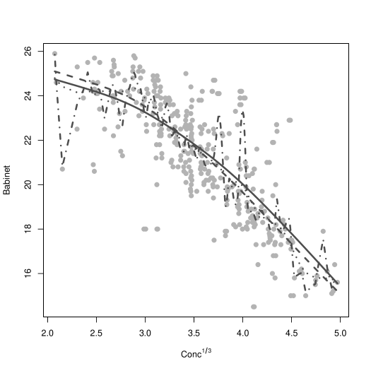
Figure 1: Robust smoothing splines fit to the Babinet data. The solid line is the classical fit, the dashed line is the M-sm1 smoothing spline, the robust-GCV-based M-smoothing spline M-sm2 is the dash-dot line, while the dotted line corresponds to the fit obtained with a subjectively chosen value of the smoothing parameter.

Figure 2 shows the S-pen (solid line) and M-loc (dashed line) fits. Note that the local linear M-estimator is less smooth than appears to be necessary, and also is slightly higher than expected for $x\approx 4$. The S-penalized spline provides both a satisfying level of smoothness and a good fit to the trend and bulk of the data. Scripts reproducing this analysis can be found in an on-line supplement.

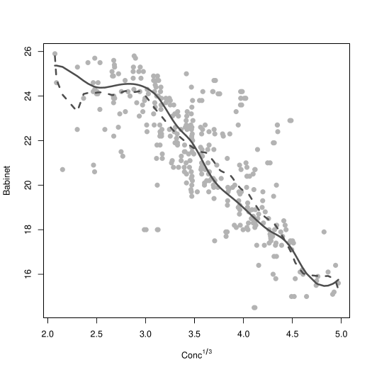
Figure 2: Robust non-parametric regression estimates for the Babinet data. The solid line is the S-penalized splines S-pen, and the dashed line is the robust local linear M-estimator M-loc.

5 Concluding remarks

In this review we focused on robust nonparametric regression estimators for models with a continuous response. We explicitly discussed the different practical advantages and limitations of each approach, including options for robust bandwidth and smoothing parameter selection. We also reviewed recently proposed methods that scale well with a growing number of covariates.

Formally quantifying the level of robustness of estimation methods for nonparametric regression models is a challenging problem. Since the “parameter” being estimated is intrinsically infinite dimensional, the “classical” measures of robustness need to be extended appropriately. Moreover, note that for example, in linear regression, damaging outliers affect all fitted values, and thus, intuitively, one prefers an estimated regression function that ignores atypical observations and provides a better fit to the other points, over an estimated regression function that may have accommodated the outliers and fit the other points notably worse. However, when the model is highly flexible, “atypical” observations may not affect the quality of the fit at other points in the training set, and thus it is hard to justify prefering a fit that ignores outliers over one that is affected by them, particularly when outliers are “isolated” (so that there are no local “good” reference points). In other words, robustness is, in fact, a concept relative to a model, and will be affected by the “richness” of the model in terms of the regression functions that can be estimated (the “flexibility of the estimator”) (see, e.g. Hable and Christmann, 2013). Further research on these issues would be a very welcome contribution to the field.

6 Acknowledgements

The author would like to thank two anonymous referees and an Associate Editor for their constructive comments on an earlier version of this work that resulted in a notably improved paper. This research was supported by the Natural Sciences and Engineering Research Council of Canada (Discovery Grant RGPIN-2016-04288).

References

- [1] Bianco, A. and Boente, G. (1998). Robust kernel estimators for additive models with dependent observations. The Canadian Journal of Statistics, 26(2), 239-255.
- [2] Bianco, A. and Boente, G. (2007). Robust estimators under a semiparametric partly linear autoregression model: asymptotic behavior and bandwidth selection. Journal of Time Series Analysis, 28, 274-306.
- [3] Boente, G. and Fraiman, R. (1989a). Robust nonparametric regression estimation. Journal of Multivariate Analysis, 29, 180-198.
- [4] Boente, G. and Fraiman, R. (1989b). Robust nonparametric regression estimation for dependent observations. The Annals of Statistics, 17(3), 1242-1256.
- [5] Boente, G. and Rodriguez, D. (2006). Robust estimators of high order derivatives of regression functions. Statistics and Probability Letters, 76, 1335-1344.
- [6] Boente, G. and Rodriguez, D. (2008). Robust bandwidth selection in semiparametric partly linear regression models: Monte Carlo study and influential analysis. Computational Statistics and Data Analysis, 52, 383-397.
- [7] Boente, G., Salibian-Barrera, M. and Vena, P. (2020). Robust estimation for semi-functional linear regression models. Computational Statistics & Data Analysis, 152. In press.
- [8] Boente, G., Fraiman, R., and Meloche, J. (1997). Robust plug-in bandwidth estimators in nonparametric regression. Journal of Statistical Planning and Inference, 57, 109-142
- [9] Boente, G. and Martinez, A. (2017). Marginal integration M-estimators for additive models. TEST, 26(2), 231-260.
- [10] Boente, G. and Martinez, A. (2023). A robust spline approach in partially linear additive models. Computational Statistics & Data Analysis, 178. In press.
- [11] Boente, G., Martínez, A. and Salibian-Barrera, M. (2017). Robust estimators for additive models using backfitting. Journal of Nonparametric Statistics, 29(4), 744-767.
- [12] Boente, G., Ruiz, M. and Zamar, R.H. (2010). On a robust local estimator for the scale function in heteroscedastic nonparametric regression. Statistics and Probability Letters, 80, 1185-1195.
- [13] Boente, G., Ruiz, M. and Zamar, R.H. (2012). Bandwidth choice for robust nonparametric scale function estimation. Computational Statistics and Data Analysis, 56, 1594-1608.
- [14] Breiman, L. (2001). Random Forests. Machine Learning, 45, 5-32.
- [15] Breiman, L., Friedman, J.H., Olshen, R.A. and Stone, C.J. (1984). Classification and Regression Trees. Routledge, New York.
- [16] Buja, A., Hastie, T. and Tibshirani, R. (1989). Linear smoothers and additive models (with discussion). The Annals of Statistics, 17, 453-510.
- [17] Cantoni, E., and Ronchetti, E. (2001). Resistant selection of the smoothing parameter for smoothing. Statistics and Computing, 11(2), 141-146.
- [18] Chambers, R., Hentges, A. and Zhao, X. (2004). Robust automatic methods for outlier and error detection. Journal of the Royal Statistical Society, Series A, 167(2), 323-339.
- [19] Cleveland, W.S. (1993). Visualizing Data, Summit, NJ: Hobart Press.
- [20] Cox, D.D. (1983). Asymptotics for M-type smoothing splines. The Annals of Statistics, 11(2), 530-551.
- [21] Cox, D.D. (1984). Multivariate smothing spline functions. SIAM Journal of Numerical Analysis, 21, 789-813.
- [22] Christmann, A. and Steinwart, I. (2007). Consistency and robustness of kernel-based regression in convex risk minimization. Bernoulli, 13, 799-819.
- [23] Christmann, A., Salibian-Barrera, M. and van Aelst, S. (2013). Qualitative robustness of boostrap approximations for kernel based methods. In Robustness and Complex Data Structures. Festschrift in Honour of Ursual Gather, Eds. C. Becker, S. Kuhnt, R. Fried, pages 263-278. Springer.
- [24] Cunningham, J. K., Eubank, R. L. and Hsing, T. (1991). M-type smoothing splines with auxiliary scale estimation. Computational Statistiscs & Data Analysis, 11, 43-51.
- [25] Eilers, P. and Marx, B. (1996). Flexible smoothing with B-splines and penalties (with discussion). Statistical Science, 11, 89-121.
- [26] Fan, J., Hu, T-C. and Truong, Y.K. (1994). Robust non-parametric function estimation. Scandinavian Journal of Statistics, 21(4), 433-446.
- [27] Ferraty, F. and Vieu, P. (2006). Nonparametric Functional Data Analysis: Theory and Practice. Springer.
- [28] Friedman, J.H., and Stuetzle, W. (1981). Projection pursuit regression. Journal of the American Statistical Association, 76, 817-823.
- [29] Friedman, J.H. (2001). Greedy function approximation: A gradient boosting machine. The Annals of Statistics, 29(5), 1189-1232.
- [30] Galimberti, G., Pillati, M., and Soffritti, G. (2007). Robust regression trees based on M-estimators. Statistica, 67(2), 173-190.
- [31] Gasser, T., Sroka, L. and Jennen-Steinmetz, C. (1986). Residual variance and residual pattern in nonlinear regression. Biometrika, 73, 625-633.
- [32] Ghement, I.R., Ruiz, M. and Zamar, R. (2008). Robust estimation of error scale in nonparametric regression models. Journal of Statistical Planning and Inference, 138, 3200-3216.
- [33] Giloni, A. and Simonoff, J.S. (2005). The conditional breakdown properties of least absolute value local polynomial estimators. Journal of Nonparametric Statistics, 17(1), 15-30.
- [34] Green, P.J. and Silverman, B.W. (1994) Nonparametric regression and generalized linear models, a roughness penalty approach. New York: Chapman & Hall / CRC.
- [35] Grenander, U. (1981). Abstract Inference. New York: Wiley.
- [36] Györfi, L., Kohler, M., Krzyzak, A. and Walk, H. (2010). A Distribution-Free Theory of Nonparametric Regression. New York : Springer.
- [37] Hable, R. and Christmann, A. (2011). On qualitative robustness of support vector machines. Journal of Multivariate Analysis, 102, 993-1007.
- [38] Hable, R. and Christmann, A. (2013). Robustness versus consistency in ill-posed classification and regression problems. In Classification and Data Mining. Studies in Classification, Data Analysis and Knowledge Organization, Eds. A. Giusti, G. Ritter, M. Vichi, pages 27-35. Springer.
- [39] Hall, P. and Jones, M.C. (1990). Adaptive M-estimation in nonparametric regression. The Annals of Statistics, 18(4), 1712-1728.
- [40] Härdle, W. and Gasser, T. (1984). Robust non-parametric function fitting. Journal of the Royal Statistical Society, Series B, 46(1), 42-51.
- [41] Härdle, W. and Gasser, T. (1985). On robust kernel estimation of derivatives of regression functions. Scandinavian Journal of Statistics, 12, 233-240.
- [42] Härdle, W. and Tsybakov, A.B. (1988). Robust nonparametric regression with simultaneous scale curve estimation. The Annals of Statistics, 16(1), 120-135.
- [43] Härdle, W., Müller, M., Sperlich, S., and Werwatz, A. (2004). Nonparametric and semiparametric models, Berlin: Springer.
- [44] Hart, J.D. and Yi, S. (1998). One-sided cross validation. Journal of the American Statistical Association, 93:442, 620-631.
- [45] Hastie, T.J. and Tibshirani, R.J. (1990). Generalized Additive Models. Monographs on Statistics and Applied Probability. 43. Chapman and Hall, London.
- [46] Hastie, T.J., Tibshirani, R.J. and Friedman, J. (2009). The elements of statistical learning, 2nd edition, New York : Springer.
- [47] He, X. and Shi, P. (1995). Asymptotics for M-Type Regression Splines with Auxiliary Scale Estimation. Sankhyā Series A, 57(3), 452-461.
- [48] Horowitz, J. (1998). Semiparametric Methods in Econometrics. New York : Springer.
- [49] Huber, P.J. (1979). Robust smoothing. In Proc. ARO Workshop on Robustness in Statistics, Eds. R. N. Launer and G. N. Wilkinson. New York: Academic Press.
- [50] Jiang, J. and Mack, Y.P. (2001). Robust local polynomial regression for dependent data. Statistica Sinica, 11, 705-722.
- [51] John, G.H. (1995). Robust decision trees: removing outliers in databases. In First International Conference on Knowledge Discovery and Data Mining (KDD-95), AAAI Press, Menlo Park, CA, 174-179.
- [52] Ju, X., Salibian-Barrera, M. (2021). Robust Boosting for Regression Problems. Computational Statistics and Data Science, 153. DOI: 10.1016/j.csda.2020.107065.
- [53] Kalogridis, I. (2022a). Asymptotics for M-type smoothing splines with non-smooth objective functions. TEST, 31, 373-389.
- [54] Kalogridis, I. (2022b). Robust thin-plate splines for multivariate spatial smoothing. arXiv:2207.13931.
- [55] Kalogridis, I. and Van Aelst, S. (2021). M-type penalized splines with auxiliary scale estimation. Journal of Statistical Planning and Inference, 212, 97-113.
- [56] Kalogridis, I. and Van Aelst, S. (2022). Robust penalized spline estimation with difference penalties. Econometrics and Statistics, in press.
- [57] Lee, J.S. and Cox, D.D. (2010). Robust smoothing: smoothing parameter selection and applications to fluorescence spectroscopy. Computational Statistics and Data Analysis, 54, 3131-3143..
- [58] Lee, T.C.M. and Oh, H-S. (2007). Robust penalized regression spline fitting with application to additive mixed modeling. Computational Statistics, 22, 159-171.
- [59] Leung, D.H.-Y. (2005). Cross-validation in nonparametric regression with outliers. The Annals of Statistics, 33(5), 2291-2310.
- [60] Leung, D.H.-Y., Marriot, F.H.C., and Wu, E.K.H. (1993). Bandwidth selection in robust smoothing. Journal of nonparametric statistics, 4, 333-339.
- [61] Linton, O. and Nielsen, J. (1995). A kernel method of estimating structured nonparametric regression based on marginal integration. Biometrika, 82, 93-101.
- [62] Lutz, R.W., Kalisch, M. and Bühlmann, P. (2008). Robustified boosting. Computational Statistics and Data Analysis, 52, 3331-3341.
- [63] Ma, Y. and Zhao, G. (2016). Robust nonparametric kernel regression estimator. Statistics and Probability Letters, 116, 72-79.
- [64] Maronna RA, Martin DR, Yohai VJ, Salibian-Barrera M. (2018). Robust Statistics: Theory and Methods (with R), 2nd ed. Wiley Series in Probability and Statistics. New York: John Wiley & Sons.
- [65] Nadaraya, E. A. (1964). On estimating regression. Theory of Probability and its Applications, 10, 186-190.
- [66] Oh, H-S., Nychka, D.W., Brown, T. and Charbonneau, P. (2004). Period analysis of variable stars by robust smoothing. Journal of the Royal Statistical Society, Series C, 53, 15-30.
- [67] Oh, H-S., Nychka, D.W. and Lee, T.C.M. (2007). The role of pseudo data for robust smoothing with application to wavelet regression. Biometrika, 94(4), 893-904.
- [68] R Core Team. (2022). R: A language and environment for statistical computing. R Foundation for Statistical Computing, Vienna, Austria. URL https://www.R-project.org/.
- [69] Rice, J. (1984). Bandwidth choice for nonparametric regression. The Annals of Statistics, 12, 1215-1230.
- [70] Ronchetti, E. and Staudte, R.G. (1994). A robust version of Mallows’ . Journal of the American Statistical Association, 89, 550-559.
- [71] Ruppert, D. (2002). Selecting the number of knots for penalized splines. Journal of Computational and Graphical Statistics, 11:4, 735-757.
- [72] Ruppert, D., Wand, M., and Carroll, R. (2003). Semiparametric Regression. Cambridge Series in Statistical and Probabilistic Mathematics. Cambridge: Cambridge University Press.
- [73] Shi, P. (1997). M-type regression splines involving time series. Journal of Statistical Planning and Inference, 61, 17-37.
- [74] Shi, P. and Li, G. (1995). Global convergence rates of B-spline M-estimators in nonparametric regression. Statistica Sinica, 5, 303-318.
- [75] Steinwart, I. and Christmann, A. (2008). Support Vector Machines. Springer.
- [76] Stone, C.J. (1980). Optimal rates of convergence for nonparametric estimators. The Annals of Statistics, 8, 1348-1360.
- [77] Stone, C.J. (1986). The dimensionality reduction principle for generlized additive models. The Annals of Statistics, 14, 590-606.
- [78] Tamine, J. (2002). Smoothed influence function: another view at robust nonparametric regression. Discussion paper 62. Sonderforschungsbereich 373. Humboldt-Unbersität zu Berlin.
- [79] Tharmaratnam, K., Claeskens, G., Croux, C. and Salibian-Barrera, M. (2010). S-estimation for penalized regression splines. Journal of Computational and Graphical Statistics, 19(3), 609-625.
- [80] Tjøstheim, D. and Auestad, B. (1994). Nonparametric identification of nonlinear time series: selecting significant lags. Journal of the American Statistical Association, 89, 1410-1430.
- [81] Wang, F. and Scott, D. (1994). The method for robust nonparametric regression. Journal of the American Statistical Association, 89, 65-76.
- [82] Wang, B., Shi, W. and Miao, Z. (2014). Comparative analysis for robust penalized spline smoothing methods. Mathematical Problems in Engineering, 2014.
- [83] Watson, G. S. (1964). Smooth regression analysis. Sankhyā Series A, 26, 359-372.
- [84] Welsh, A.H. (1996). Robust estimation of smooth regression and spread functions and their derivatives. Statistica Sinica, 6, 347-366.
- [85] Wood, S.N. (2000). Modelling and Smoothing Parameter Estimation with Multiple Quadratic Penalties. Journal of the Royal Statistical Society, Series B 62:2, 413-428
- [86] Wood, S.N. (2006). Generalized Additive Models. Boca Raton : Chapman & Hall / CRC.
- [87] Wood, S.N., Pya, N. and Säfken, B. (2016) Smoothing Parameter and Model Selection for General Smooth Models, Journal of the American Statistical Association, 111:516, 1548-1563,
- [88] Xiao, L. (2019). Asymptotic theory of penalized splines. Electronic Journal of Statistics, 13(1), 747-794.
- [89] Yuan, M. (2011). On the identifiability of additive index models. Statistica Sinica, 21, 1901-1911.