Stability and convergence of the Euler scheme for stochastic linear evolution equations in Banach spaces

Abstract

For the Euler scheme of the stochastic linear evolution equations, discrete stochastic maximal $L^{p}$-regularity estimate is established, and a sharp error estimate in the norm $\lVert{\cdot}\rVert_{L^{p}((0,T)\times\Omega;L^{q}(\mathcal{O}))}$, $p,q\in[2,\infty)$, is derived via a duality argument.

Keywords: stochastic evolution equations, Euler scheme, discrete stochastic maximal $L^{p}$-regularity, convergence

1 Introduction

The numerical methods of stochastic partial differential equations have been extensively studied in the past decades, and by now it is still an active research area; see, e.g., [1, 3, 4, 5, 6, 7, 13, 23, 24]. However, the numerical analysis in this field so far mainly focuses on the Hilbert space setting; the numerical analysis of the Banach space setting is rather limited. This motivates us to analyze the stability and convergence of the Euler scheme for the stochastic linear evolution equations in Banach spaces, which is one of the most popular temporal discretization scheme in this realm.

Firstly, we establish a discrete stochastic maximal $L^{p}$-regularity estimate. Maximal $L^{p}$-regularity is of fundamental importance for the deterministic evolution equations; see, e.g., [8, 14, 18, 22]. In the past twenty years, the discrete maximal $L^{p}$-regularity of deterministic evolution equations has also attracted great attention; see, e.g., [2, 10, 12, 11, 15, 16, 17]. Using the techniques of $H^{\infty}$-calculus, $\mathcal{R}$-bundedness, and square function estimates, in the case of $p\in(2,\infty)$ and $q\in[2,\infty)$, Van Neerven et al. [21] established the stochastic maximal $L^{p}$-regularity estimate

$$\lVert{A^{1/2}y}\rVert_{L^{p}(\mathbb{R}_{+}\times\Omega;L^{q}(\mathcal{O}))}\leqslant c\lVert{f}\rVert_{L^{p}(\mathbb{R}_{+}\times\Omega;L^{q}(\mathcal{O};H))},$$

for the stochastic linear evolution equation

$$\begin{cases}\mathrm{d}y+Ay(t)\,\mathrm{d}t=f(t)\,\mathrm{d}W(t),\quad t>0,\\ y(0)=0.\end{cases}$$

Following the idea in [21], for the Euler scheme

$$\begin{cases}Y_{j+1}-Y_{j}+\tau AY_{j+1}=f_{j}\delta W_{j},\quad j\in\mathbb{N},\\ Y_{0}=0,\end{cases}$$

we obtain the discrete stochastic maximal $L^{p}$-regularity estimate

$$\Big{(}\sum_{j=0}^{\infty}\Big{\lVert}{\frac{Y_{j+1}-Y_{j}}{\sqrt{\tau}}}\Big{\rVert}_{L^{p}(\Omega;L^{q}(\mathcal{O}))}^{p}\Big{)}^{1/p}+\Big{(}\sum_{j=0}^{\infty}\lVert{A^{1/2}Y_{j}}\rVert_{L^{q}(\mathcal{O})}^{p}\Big{)}^{1/p}$$

$$\leqslant{} c\Big{(}\sum_{j=0}^{\infty}\lVert{f_{j}}\rVert_{L^{p}(\Omega;L^{q}(\mathcal{O};H))}^{p}\Big{)}^{1/p}.$$

Under the condition that $p=q=2$ and ${-A}$ is the realization of the Laplace operator in $L^{q}(\mathcal{O})$ with homogeneous Dirichlet boundary condition, the above estimate can be proved by a straightforward energy argument. Although our numerical analysis assumes that $A$ is a sectorial operator on $L^{q}(\mathcal{O})$, it can also be extended to the Stokes operator.

Secondly, we derive a sharp error estimate in the norm $\lVert{\cdot}\rVert_{L^{p}((0,T)\times\Omega;L^{q}(\mathcal{O}))}$, $p,q\in[2,\infty)$. So far, the numerical analysis in the literature mainly considers the convergence in a Hilbert space at some given points of time; the convergence in the norm $L^{p}((0,T)\times\Omega;L^{q}(\mathcal{O}))$ has rarely been analyzed. Error estimates of this type not only characterize intrinsically the convergence of the Euler scheme, but also will be indispensable for the numerical analysis of optimal control problems governed by the stochastic evolution equations. We use a duality argument, together with the convergence result of a discrete deterministic evolution equation, to derive a sharp error estimate

$$\Big{(}\sum_{j=0}^{J-1}\lVert{y-Y_{j}}\rVert_{L^{p}((t_{j},t_{j+1})\times\Omega;L^{q}(\mathcal{O}))}^{p}\Big{)}^{1/p}\leqslant c\tau^{1/2}\lVert{f}\rVert_{L^{p}((0,T)\times\Omega;L^{q}(\mathcal{O};H))}.$$

As far as we know, in the case of $p=q=2$ (i.e., a Hilbert space setting), the above error estimate is still new.

The rest of this paper is organized as follows. Section 2 introduces some notations and the concepts of $\gamma$-radonifying operators, $\mathcal{R}$-boundedness, $H^{\infty}$-calculus and stochastic integral. Section 3 establishes the discrete maximal $L^{p}$-regularity. Section 4 derives a sharp convergence rate.

2 Preliminaries

Conventions. Throughout this paper, we will use the following conventions: for a Banach space $E$, $\langle{\cdot,\cdot}\rangle_{E}$ denotes the duality pairing between $E$ and its dual space $E^{*}$; for any Banach spaces $E_{1}$ and $E_{2}$, $\mathcal{L}(E_{1},E_{2})$ denotes the set of all bounded linear operators from $E_{1}$ to $E_{2}$, and $\mathcal{L}(E_{1},E_{1})$ is abbreviated to $\mathcal{L}(E_{1})$; for any $p\in[1,\infty)$, $p^{\prime}$ denotes the conjugate exponent of $p$; $\mathcal{O}\subset\mathbb{R}^{d}\,(d\geqslant 2)$ is a bounded domain with $C^{2}$-boundary; $i$ denotes the imaginary unit; by $c$ we mean a generic positive constant, which is independent of the time step $\tau$ but may differ in different places. In addition, for any $\theta\in(0,\pi)$,

$$\Sigma_{\theta}:=\{z\in\mathbb{C}\setminus\{0\}\mid\,\lvert{\operatorname{Arg}z}\rvert<\theta\},$$

where the argument of each complex scalar takes value in $(-\pi,\pi]$.

$\gamma$-Radonifying operators. For any Banach space $E$ and Hilbert space $U$ with inner product $(\cdot,\cdot)_{U}$, define

$$\mathcal{S}(U,E):=\text{span}\big{\{}u\otimes e\mid\,u\in U,\,e\in E\},$$

where $u\otimes e\in\mathcal{L}(U,E)$ is defined by

$$(u\otimes e)(v):=(v,u)_{U}e,\quad\forall v\in U.$$

Let $\gamma(U,E)$ denote the completion of $\mathcal{S}(U,E)$ with respect to the norm

$$\Big{\lVert}{\sum_{n=1}^{N}\phi_{n}\otimes e_{n}}\Big{\rVert}_{\gamma(U,E)}:=\Big{(}\mathbb{E}\Big{\lVert}{\sum_{n=1}^{N}\gamma_{n}e_{n}}\Big{\rVert}_{E}^{2}\Big{)}^{1/2}$$

for all $N\in\mathbb{N}_{>0}$, all orthonormal systems $(\phi_{n})_{n=1}^{N}$ of $U$, all sequences $(e_{n})_{n=1}^{N}$ in $E$, and all sequences $(\gamma_{n})_{n=1}^{N}$ of independent standard Gaussian random variables, where $\mathbb{E}$ denotes the expectation operator associated with the probability space on which $\gamma_{1},\ldots,\gamma_{N}$ are defined.

$\mathcal{R}$-boundedness. For any two Banach spaces $E_{1}$ and $E_{2}$, an operator family $\mathcal{A}\subset\mathcal{L}(E_{1},E_{2})$ is said to be $\mathcal{R}$-bounded if there exists a constant $C>0$ such that

$$\int_{0}^{1}\Big{\lVert}{\sum_{n=1}^{N}r_{n}(t)B_{n}x_{n}}\Big{\rVert}_{E_{2}}^{2}\,\mathrm{d}t\leqslant C\int_{0}^{1}\Big{\lVert}{\sum_{n=1}^{N}r_{n}(t)x_{n}}\Big{\rVert}_{E_{1}}^{2}\,\mathrm{d}t$$

for all $N\geqslant 1$, all sequences $(B_{n})_{n=1}^{N}$ in $\mathcal{A}$, all sequences $(x_{n})_{n=1}^{N}$ in $E_{1}$, and all sequences $(r_{n})_{n=1}^{N}$ of independent symmetric $\{-1,1\}$-valued random variables on $[0,1]$. We denote by $\mathcal{R}(\mathcal{A})$ the infimum of these $C$’s.

$H^{\infty}$-calculus. A sectorial operator $A$ on some Banach space $E$ is said to have a bounded $H^{\infty}$-calculus if there exists $\sigma\in(0,\pi]$ such that

$$\Big{\lVert}{\int_{\partial\Sigma_{\sigma}}\Psi(z)(z-A)^{-1}\,\mathrm{d}z}\Big{\rVert}_{\mathcal{L}(E)}\leqslant C\sup_{z\in\Sigma_{\sigma}}\lvert{\Psi(z)}\rvert$$

for all $\varphi\in\mathcal{H}_{0}^{\infty}(\Sigma_{\sigma})$, where $C$ is a positive constant independent of $\varphi$ and

$$\mathcal{H}_{0}^{\infty}(\Sigma_{\sigma}) :=\Big{\{}\varphi:\Sigma_{\sigma}\to\mathbb{C}\mid\,\text{$\varphi$ is analytic and there exists $\varepsilon>0$ such that}$$

$$\qquad\qquad\qquad\qquad\qquad\sup_{z\in\Sigma_{\sigma}}\Big{(}\frac{1+\lvert{z}\rvert^{2}}{\lvert{z}\rvert}\Big{)}^{\varepsilon}\lvert{\Psi(z)}\rvert<\infty\Big{\}}.$$

The infimum of these $\sigma$’s is called the angle of the $H^{\infty}$-calculus of $A$.

Stochastic integral. Assume that $(\Omega,\mathcal{F},\mathbb{P})$ is a given complete probability space with a filtration $\mathbb{F}:=(\mathcal{F}_{t})_{t\geqslant 0}$, on which a sequence of independent $\mathbb{F}$-adapted Brownian motions $(\beta_{n})_{n\in\mathbb{N}}$ are defined. In the sequel, we will use $\mathbb{E}$ to denote the expectation of a random variable on $\Omega$. Let $H$ be a separable Hilbert space with inner product $(\cdot,\cdot)_{H}$ and an orthonormal basis $(h_{n})_{n\in\mathbb{N}}$. For each $t\in\mathbb{R}_{+}$, define $W(t)\in\mathcal{L}(H,L^{2}(\Omega))$ by

$$W(t)h:=\sum_{n\in\mathbb{N}}\beta_{n}(t)(h,h_{n})_{H},\quad\forall h\in H.$$

Assume that $p,q\in(1,\infty)$. For any

$$f=\sum_{l=1}^{L}\sum_{m=1}^{M}\sum_{n=1}^{N}I_{(t_{l-1},t_{l}]}g_{lmn}h_{n},$$

define

$$\int_{\mathbb{R}_{+}}f(t)\,\mathrm{d}W(t):=\sum_{l=1}^{L}\sum_{m=1}^{M}\sum_{n=1}^{N}\big{(}\beta_{n}(t_{l})-\beta_{n}(t_{l-1})\big{)}g_{lmn},$$

where $L,M,N$ are positive integers, $0\leqslant t_{0}\leqslant t_{1}\ldots\leqslant t_{L}<\infty$, $I_{(t_{l-1},t_{l}]}$ is the indicator function of the time interval $(t_{l-1},t_{l}]$, and

$$g_{lmn}\in L^{p}(\Omega,\mathcal{F}_{t_{l-1}},\mathbb{P};L^{q}(\mathcal{O})).$$

We denote by $\mathcal{S}_{pq}$ the set of all such functions $f$’s. The above integral has the following essential isomorphism feature; see, e.g., [20, Theorem 2.3].

Lemma 2.1.

For any $p,q\in(1,\infty)$, there exist two positive constants $c_{0}$ and $c_{1}$ such that

$$c_{0}\mathbb{E}\lVert{f}\rVert_{L^{q}(\mathcal{O};L^{2}(\mathbb{R}_{+};H))}^{p}\leqslant\mathbb{E}\Big{\lVert}{\int_{\mathbb{R}_{+}}f(t)dW(t)}\Big{\rVert}_{L^{q}(\mathcal{O})}^{p}\leqslant c_{1}\mathbb{E}\lVert{f}\rVert_{L^{q}(\mathcal{O};L^{2}(\mathbb{R}_{+};H))}^{p}$$ (1)

for all $f\in\mathcal{S}_{pq}$.

By virtue of this lemma, for any $p,q\in(1,\infty)$, the above integral can be uniquely extended to the space $L_{\mathbb{F}}^{p}(\Omega;L^{q}(\mathcal{O};L^{2}(\mathbb{R}_{+};H)))$, defined as the closure of $\mathcal{S}_{pq}$ in $L^{p}(\Omega;L^{q}(\mathcal{O};L^{2}(\mathbb{R}_{+};H)))$. For any $p\in(1,\infty)$ and $q\in[2,\infty)$, since Minkowski’s inequality implies

$$\lVert{f}\rVert_{L^{p}(\Omega;L^{q}(\mathcal{O};L^{2}(\mathbb{R}_{+};H)))}\leqslant\lVert{f}\rVert_{L^{p}(\Omega;L^{2}(\mathbb{R}_{+};L^{q}(\mathcal{O};H))}\quad\forall f\in\mathcal{S}_{pq},$$

the above integral can also be uniquely extended to $L_{\mathbb{F}}^{p}(\Omega;L^{2}(\mathbb{R}_{+};L^{q}(\mathcal{O};H)))$, defined as the closure of $\mathcal{S}_{pq}$ in $L^{p}(\Omega;L^{2}(\mathbb{R}_{+};L^{q}(\mathcal{O};H)))$.

Discrete spaces. For any Banach space $E$ and $p\in[1,\infty)$, define

$$\ell^{p}(E):=\Big{\{}(v_{j})_{j\in\mathbb{N}}\Bigl{|}\,\,\sum_{j\in\mathbb{N}}\lVert{v_{j}}\rVert_{E}^{p}<\infty\Big{\}},$$

and endow this space with the norm

$$\lVert{(v_{j})_{j\in\mathbb{N}}}\rVert_{\ell^{p}(E)}:=\Big{(}\sum_{j\in\mathbb{N}}\lVert{v_{j}}\rVert_{E}^{p}\Big{)}^{1/p}\quad\text{for all }(v_{j})_{j\in\mathbb{N}}\in\ell^{p}(E).$$

For any $v\in\ell^{p}(E)$, we use $v_{j}$, $j\in\mathbb{N}$, to denote its $j$-th element.

3 Stability estimates

Fix $0<\tau<1$ and let $t_{j}:=j\tau$ for each $j\in\mathbb{N}$. Define

$$\delta W_{j}:=W(t_{j+1})-W(t_{j}),\quad j\in\mathbb{N}.$$

For any $p,q,r\in[1,\infty)$, define

$$\ell_{\mathbb{F}}^{p}(L^{r}(\Omega;L^{q}(\mathcal{O};H))):=\big{\{}v\in\ell^{p}(L^{r}(\Omega;L^{q}(\mathcal{O};H)))\mid\,v_{j}\text{ is $\mathcal{F}_{t_{j}}$-measurable}\big{\}}.$$

It is standard that $\ell_{\mathbb{F}}^{p}(L^{r}(\Omega;L^{q}(\mathcal{O};H)))$ is a Banach space with respect to the norm $\lVert{\cdot}\rVert_{\ell^{p}(L^{r}(\Omega;L^{q}(\mathcal{O};H)))}$. This section studies the stability of the following Euler scheme: seek $Y:=(Y_{j})_{j\in\mathbb{N}}$ such that

$$Y_{j+1}-Y_{j}+\tau AY_{j+1}=f_{j}\delta W_{j},\quad j\in\mathbb{N},$$ (2a)

$$Y_{0}=0,$$ (2b)

where $f:=(f_{j})_{j\in\mathbb{N}}$ is given. The main result of this section are the following two theorems.

Theorem 3.1.

Let $p,q,r\in(1,\infty)$. Assume that $A$ is a densely defined sectorial operator on $L^{q}(\mathcal{O})$ and

$$\mathcal{R}\big{(}\{z(z-A)^{-1}\mid z\in\mathbb{C}\setminus\Sigma_{\theta_{A}}\}\big{)}<\infty,$$ (3)

where $\theta_{A}\in(0,\pi/2)$. Let $Y$ be the solution to 2 with

$$f\in\ell_{\mathbb{F}}^{p}(L^{r}(\Omega;L^{q}(\mathcal{O};H))).$$

Then

$$\Big{(}\sum_{j=0}^{\infty}\Big{\lVert}{\frac{Y_{j+1}-Y_{j}}{\sqrt{\tau}}}\Big{\rVert}_{L^{r}(\Omega;L^{q}(\mathcal{O}))}^{p}\Big{)}^{1/p}\leqslant c\lVert{f}\rVert_{\ell^{p}(L^{r}(\Omega;L^{q}(\mathcal{O};H)))}.$$ (4)

Theorem 3.2.

Let $p\in(2,\infty)$ and $q\in[2,\infty)$. Assume that $A$ is a densely defined sectorial operator on $L^{q}(\mathcal{O})$ satisfying the following conditions:

• the range of $A$ is dense in $L^{q}(\mathcal{O})$;

• the resolvent set of $A$ contains $\{z\in\mathbb{C}\setminus\{0\}\mid\lvert{\operatorname{Arg}z}\rvert\geqslant\theta_{A}\}$ with $\theta_{A}\in(0,\pi/2)$;

• $$\sup_{z\in\mathbb{C}\setminus\{0\},\,\lvert{\operatorname{Arg}z}\rvert\geqslant\theta_{A}}\,\lvert{z}\rvert\lVert{(z-A)^{-1}}\rVert_{\mathcal{L}(L^{q}(\mathcal{O}))}<\infty;$$ (5)

• $A$ admits a bounded $H^{\infty}$-calculus of angle less than $\theta_{A}$.

Let $Y$ be the solution to 2 with

$$f\in\ell_{\mathbb{F}}^{p}(L^{p}(\Omega;L^{q}(\mathcal{O};H))).$$

Then

$$\lVert{A^{1/2}Y}\rVert_{\ell^{p}(L^{p}(\Omega;L^{q}(\mathcal{O})))}\leqslant c\lVert{f}\rVert_{\ell^{p}(L^{p}(\Omega;L^{q}(\mathcal{O};H)))}.$$ (6)

3.1 Proof of Theorem 3.1

Assume that each $f_{j}$ is of the form

$$f_{j}=\sum_{m=1}^{M}\sum_{n=1}^{N}g_{jmn}h_{n},$$

where $M,N$ are positive integers and $g_{jmn}\in L^{p}(\Omega,\mathcal{F}_{t_{j}},\mathbb{P};L^{q}(\mathcal{O}))$; the general case can be proved by a density argument. Let $\widetilde{A}$ be the natural extension of $A$ in $L^{r}(\Omega;L^{q}(\Omega))$. It is easily verified that $\widetilde{A}$ is a sectorial operator on $L^{r}(\Omega;L^{q}(\Omega))$. Let $(r_{n})_{n=1}^{\infty}$ be a sequence of independent symmetric $\{-1,1\}$-valued random variables on $[0,1]$. For any $N\geqslant 1$, $(z_{n})_{n=1}^{N}\subset\Sigma_{\pi-\theta_{A}}$ and $(v_{n})_{n=1}^{N}\subset L^{r}(\Omega;L^{q}(\mathcal{O}))$, we obtain

$$\Big{(}\int_{0}^{1}\Big{\lVert}{\sum_{n=1}^{N}r_{n}(t)z_{n}(z_{n}+\widetilde{A})^{-1}v_{n}}\Big{\rVert}_{L^{r}(\Omega;L^{q}(\mathcal{O}))}^{2}\,\mathrm{d}t\Big{)}^{1/2}$$

$$\stackrel{{\scriptstyle\text{(i)}}}{{\leqslant}} c\Big{(}\int_{0}^{1}\Big{\lVert}{\sum_{n=1}^{N}r_{n}(t)z_{n}(z_{n}+\widetilde{A})^{-1}v_{n}}\Big{\rVert}_{L^{r}(\Omega;L^{q}(\mathcal{O}))}^{r}\,\mathrm{d}t\Big{)}^{1/r}$$

$$={} c\Big{(}\mathbb{E}\int_{0}^{1}\Big{\lVert}{\sum_{n=1}^{N}r_{n}(t)z_{n}(z_{n}+\widetilde{A})^{-1}v_{n}}\Big{\rVert}_{L^{q}(\mathcal{O})}^{r}\,\mathrm{d}t\Big{)}^{1/r}$$

$$={} c\Big{(}\mathbb{E}\int_{0}^{1}\Big{\lVert}{\sum_{n=1}^{N}r_{n}(t)z_{n}(z_{n}+A)^{-1}v_{n}}\Big{\rVert}_{L^{q}(\mathcal{O})}^{r}\,\mathrm{d}t\Big{)}^{1/r}$$

$$\stackrel{{\scriptstyle\text{(ii)}}}{{\leqslant}} c\bigg{(}\mathbb{E}\Big{(}\int_{0}^{1}\Big{\lVert}{\sum_{n=1}^{N}r_{n}(t)z_{n}(z_{n}+A)^{-1}v_{n}}\Big{\rVert}_{L^{q}(\mathcal{O})}^{2}\,\mathrm{d}t\Big{)}^{r/2}\bigg{)}^{1/r}$$

$$\stackrel{{\scriptstyle\text{(iii)}}}{{\leqslant}} c\mathcal{R}\big{(}\{z(z+A)^{-1}\mid z\in\Sigma_{\pi-\theta_{A}}\}\big{)}\bigg{(}\mathbb{E}\Big{(}\int_{0}^{1}\Big{\lVert}{\sum_{n=1}^{N}r_{n}(t)v_{n}}\Big{\rVert}_{L^{q}(\mathcal{O})}^{2}\,\mathrm{d}t\Big{)}^{r/2}\bigg{)}^{1/r}$$

$$\stackrel{{\scriptstyle\text{(iv)}}}{{\leqslant}} c\mathcal{R}\big{(}\{z(z+A)^{-1}\mid z\in\Sigma_{\pi-\theta_{A}}\}\big{)}\Big{(}\mathbb{E}\int_{0}^{1}\Big{\lVert}{\sum_{n=1}^{N}r_{n}(t)v_{n}}\Big{\rVert}_{L^{q}(\mathcal{O})}^{r}\,\mathrm{d}t\Big{)}^{1/r}$$

$$={} c\mathcal{R}\big{(}\{z(z+A)^{-1}\mid z\in\Sigma_{\pi-\theta_{A}}\}\big{)}\Big{(}\int_{0}^{1}\Big{\lVert}{\sum_{n=1}^{N}r_{n}(t)v_{n}}\Big{\rVert}_{L^{r}(\Omega;L^{q}(\mathcal{O}))}^{r}\,\mathrm{d}t\Big{)}^{1/r}$$

$$\stackrel{{\scriptstyle\text{(v)}}}{{\leqslant}} c\mathcal{R}\big{(}\{z(z+A)^{-1}\mid z\in\Sigma_{\pi-\theta_{A}}\}\big{)}\Big{(}\int_{0}^{1}\Big{\lVert}{\sum_{n=1}^{N}r_{n}(t)v_{n}}\Big{\rVert}_{L^{r}(\Omega;L^{q}(\mathcal{O}))}^{2}\,\mathrm{d}t\Big{)}^{1/2},$$

where in (i), (ii), (iv) and (v) we used the Kahane-Khintchine inequality (see, e.g., [9, Theorem 6.2.4]), and in (iii) we used the $\mathcal{R}$-boundedness of $\{z(z+A)\mid z\in\Sigma_{\pi-\theta_{A}}\}$. It follows that $\{z(z+\widetilde{A})^{-1}\mid z\in\Sigma_{\pi-\theta_{A}}\}$ is $\mathcal{R}$-bounded. Moreover, [9, Proposition 4.2.15] implies that $L^{r}(\Omega;L^{q}(\mathcal{O}))$ is a UMD space. Therefore, we use [10, Theorem 3.2] to conclude that

$$\Big{(}\sum_{j=0}^{\infty}\Big{\lVert}{\frac{Y_{j+1}-Y_{j}}{\tau}}\Big{\rVert}_{L^{r}(\Omega;L^{q}(\mathcal{O}))}^{p}\Big{)}^{1/p}\leqslant c\Big{(}\sum_{j=0}^{\infty}\Big{\lVert}{\frac{f_{j}}{\tau}\delta W_{j}}\Big{\rVert}_{L^{r}(\Omega;L^{q}(\mathcal{O}))}^{p}\Big{)}^{1/p},$$

which implies

$$\Big{(}\sum_{j=0}^{\infty}\Big{\lVert}{\frac{Y_{j+1}-Y_{j}}{\sqrt{\tau}}}\Big{\rVert}_{L^{r}(\Omega;L^{q}(\mathcal{O}))}^{p}\Big{)}^{1/p}\leqslant c\Big{(}\sum_{j=0}^{\infty}\Big{\lVert}{\frac{f_{j}}{\sqrt{\tau}}\delta W_{j}}\Big{\rVert}_{L^{r}(\Omega;L^{q}(\mathcal{O}))}^{p}\Big{)}^{1/p}.$$

Consequently, the desired inequality 4 follows from the estimate

$$\bigg{(}\sum_{j=0}^{\infty}\Big{\lVert}{\frac{f_{j}}{\sqrt{\tau}}\delta W_{j}}\Big{\rVert}_{L^{r}(\Omega;L^{q}(\mathcal{O}))}^{p}\bigg{)}^{1/p}$$

$$\leqslant{} c\bigg{(}\sum_{j=0}^{\infty}\lVert{f_{j}}\rVert_{L^{r}(\Omega;L^{q}(\mathcal{O};H))}^{p}\bigg{)}^{1/p}\quad\text{(by \lx@cref{creftype~refnum}{lem:integral})}$$

$$={} c\lVert{f}\rVert_{\ell^{p}(L^{r}(\Omega;L^{q}(\mathcal{O};H)))}.$$

This completes the proof of Theorem 3.1.

3.2 Proof of Theorem 3.2

Throughout this subsection, we will assume that the conditions in Theorem 3.2 hold. Firstly, let us introduce some notations. Let $A^{*}$ be the dual operator of $A$ on $L^{q^{\prime}}(\mathcal{O})$. It is standard that $A^{*}$ is a sectorial operator on $L^{q^{\prime}}(\mathcal{O})$; see, e.g., [19, Theorem 2.4.1]. Moreover, $A^{*}$ has a bounded $H^{\infty}$-calculus as $A$; see [9, Proposition 10.2.20]. There exist $r_{A}>0$, $\alpha_{A}\in(\theta_{A},\pi/2)$ and $\beta_{A}\in(\pi/2,\pi)$ such that

$$\lvert{\operatorname{Arg}(e^{-z}-1)}\rvert\geqslant\alpha_{A}\quad\text{for all}\quad z\in\big{(}\Upsilon_{1}\cup\Upsilon_{2}\big{)}\setminus\{0\},$$

and that

$$\inf_{z\in\Upsilon_{2}}\inf_{\lambda\in\partial\Sigma_{\theta_{A}}}\lvert{e^{-z}-1-\lambda}\rvert>0,$$ (7)

where

$$\Upsilon_{1} :=\big{\{}-\log(1+re^{i\alpha_{A}})\mid r\in[0,r_{A}]\big{\}}\cup\big{\{}-\log(1+re^{-i\alpha_{A}})\mid r\in[0,r_{A}]\big{\}},$$

$$\Upsilon_{2} :=\Big{\{}re^{i\beta_{A}}\mid\lvert{\log(1+r_{A}e^{i\alpha_{A}})}\rvert\leqslant r\leqslant\frac{\pi}{\cos(\beta_{A}-\pi/2)}\Big{\}}$$

$$\qquad\qquad\bigcup\,\Big{\{}re^{-i\beta_{A}}\mid\lvert{\log(1+r_{A}e^{i\alpha_{A}})}\rvert\leqslant r\leqslant\frac{\pi}{\cos(\beta_{A}-\pi/2)}\Big{\}}.$$

Let $\Upsilon=\Upsilon_{1}\cup\Upsilon_{2}$. For any $z\in\Sigma_{\theta_{A}}$, define

$$\varphi_{+}(z) :=(2\pi i)^{-1/2}e^{i\alpha_{A}/4}z^{1/4}(-e^{i\alpha_{A}}+z)^{-1/2},$$ (8)

$$\varphi_{+}^{*}(z) :=(-2\pi i)^{-1/2}e^{-i\alpha_{A}/4}z^{1/4}(-e^{-i\alpha_{A}}+z)^{-1/2},$$ (9)

$$\varphi_{-}(z) :=(-2\pi i)^{-1/2}e^{-i\alpha_{A}/4}z^{1/4}(-e^{-i\alpha_{A}}+z)^{-1/2},$$ (10)

$$\varphi_{-}^{*}(z) :=(2\pi i)^{-1/2}e^{i\alpha_{A}/4}z^{1/4}(-e^{i\alpha_{A}}+z)^{-1/2}.$$ (11)

For any $z\in\Upsilon\setminus\{0\}$, define

$$\Psi(z) :=(2\pi i)^{-1/2}(e^{-z}-1)^{-1/4}(\tau A)^{1/4}(1-e^{-z}+\tau A)^{-1/2},$$ (12)

$$\Psi^{*}(z) :=(-2\pi i)^{-1/2}(e^{-\bar{z}}-1)^{-1/4}(\tau A^{*})^{1/4}(1-e^{-\bar{z}}+\tau A^{*})^{-1/2}.$$ (13)

We also define

$$\{\mathcal{I}(z):z\in\Upsilon\}\subset\mathcal{L}\big{(}\ell_{\mathbb{F}}^{p}(L^{p}(\Omega;L^{q}(\mathcal{O};H))),\,\ell^{p}(L^{p}(\Omega;L^{q}(\mathcal{O})))\big{)}$$

as follows: for any $z\in\Upsilon$ and $g\in\ell_{\mathbb{F}}^{p}(L^{p}(\Omega;L^{q}(\mathcal{O};H)))$, let

$$\big{(}\mathcal{I}(z)g\big{)}_{0}:=0,$$ (14a)

$$\big{(}\mathcal{I}(z)g\big{)}_{j}:=\sum_{k=0}^{j-1}(e^{-z}-1)^{1/2}e^{(j-k-1)z}g_{k}\frac{\delta W_{k}}{\sqrt{\tau}},\quad j\geqslant 1.$$ (14b)

In addition, for any $r\geqslant\tau/r_{A}$, let

$$\mathscr{I}_{+}(r) :=\mathcal{I}\big{(}-\log(\tau e^{i\alpha_{A}}/r+1)\big{)},$$ (15)

$$\mathscr{I}_{-}(r) :=\mathcal{I}\big{(}-\log(\tau e^{-i\alpha_{A}}/r+1)\big{)}.$$ (16)

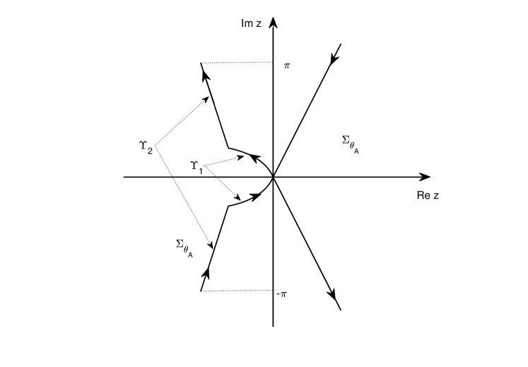
Figure 1:

Secondly, let us introduce the $\mathcal{R}$-boundedness of $\{\mathcal{I}(z)\mid z\in\Upsilon\}$ and the square function bounds associated with $\varphi_{+}$, $\varphi_{+}^{*}$, $\varphi_{-}$, $\varphi_{-}^{*}$, $\Psi$ and $\Psi^{*}$. For the clarity of the presentation of the main idea of the proof of Theorem 3.2, we put some technical lemmas in Appendix A.

Lemma 3.1.

The set $\{\mathcal{I}(z):\,z\in\Upsilon\}$ is $\mathcal{R}$-bounded.

Proof.

Define

$$\{\Pi_{m}:\,m\in\mathbb{N}\}\subset\mathcal{L}\big{(}\ell_{\mathbb{F}}^{p}(L^{p}(\Omega;L^{q}(\mathcal{O};H))),\,\ell^{p}(L^{p}(\Omega;L^{q}(\mathcal{O})))\big{)}$$

as follows: for each $m\in\mathbb{N}$ and $g\in\ell_{\mathbb{F}}^{p}(L^{p}(\Omega;L^{q}(\mathcal{O};H)))$, let

$$(\Pi_{m}g)_{0}:=0,$$ (17a)

$$(\Pi_{m}g)_{j}:=\frac{1}{\sqrt{m+1}}\sum_{k=(j-1-m)\vee 0}^{j-1}g_{k}\frac{\delta W_{k}}{\sqrt{\tau}},\quad j\geqslant 1.$$ (17b)

For any $z\in\Upsilon$ and $g\in\ell_{\mathbb{F}}^{p}(L^{p}(\Omega;L^{q}(\mathcal{O};H)))$, by definition we have

$$\big{(}\mathcal{I}(z)g\big{)}_{j} =\sum_{k=0}^{j-1}(e^{-z}-1)^{1/2}(1-e^{z})\sum_{m=j-1-k}^{\infty}e^{mz}\,g_{k}\delta W_{k}/\sqrt{\tau}$$

$$=\sum_{m=0}^{\infty}(e^{-z}-1)^{1/2}(1-e^{z})e^{mz}\sum_{k=(j-1-m)\vee 0}^{j-1}g_{k}\delta W_{k}/\sqrt{\tau}$$

$$=\sum_{m=0}^{\infty}(e^{-z}-1)^{3/2}e^{(m+1)z}\sum_{k=(j-1-m)\vee 0}^{j-1}g_{k}\delta W_{k}/\sqrt{\tau}$$

$$=\sum_{m=0}^{\infty}\sqrt{1+m}\,(e^{-z}-1)^{3/2}e^{(m+1)z}\frac{1}{\sqrt{1+m}}\sum_{k=(j-1-m)\vee 0}^{j-1}g_{k}\delta W_{k}/\sqrt{\tau}$$

$$=\sum_{m=0}^{\infty}\sqrt{1+m}\,(e^{-z}-1)^{3/2}e^{(m+1)z}(\Pi_{m}g)_{j},\quad\forall j\in\mathbb{N}_{>0}.$$

It follows that

$$\mathcal{I}(z)=\sum_{m=0}^{\infty}\sqrt{1+m}\,(e^{-z}-1)^{3/2}e^{(m+1)z}\,\Pi_{m},\quad\forall z\in\Upsilon.$$

An elementary calculation gives

$$\sup_{z\in\Upsilon}\,\sum_{m=0}^{\infty}\sqrt{m+1}\,\big{\lvert}{(e^{-z}-1)^{3/2}e^{(m+1)z}}\big{\rvert}$$

$$={} \sup_{z\in\Upsilon}\,\lvert{e^{-z}-1}\rvert^{3/2}\sum_{m=0}^{\infty}\sqrt{m+1}\,\lvert{e^{z}}\rvert^{m+1}$$

$$\leqslant{} \sup_{z\in\Upsilon}\,\lvert{e^{-z}-1}\rvert^{3/2}\int_{0}^{\infty}\sqrt{x+1}\,\lvert{e^{z}}\rvert^{x}\,\mathrm{d}x$$

$$={} \sup_{z\in\Upsilon}\,\lvert{e^{-z}-1}\rvert^{3/2}\int_{0}^{\infty}\sqrt{x+1}\,e^{x\ln\lvert{e^{z}}\rvert}\,\mathrm{d}x$$

$$={} \sup_{z\in\Upsilon}\,\frac{\lvert{e^{-z}-1}\rvert^{3/2}}{\ln\lvert{e^{-z}}\rvert}\int_{0}^{\infty}\sqrt{1+\frac{y}{\ln\lvert{e^{-z}}\rvert}}\,e^{-y}\,\mathrm{d}y$$

$$={} \sup_{z\in\Upsilon}\frac{\lvert{e^{-z}-1}\rvert}{\ln\lvert{e^{-z}}\rvert}\int_{0}^{\infty}\sqrt{\lvert{e^{-z}-1}\rvert+\frac{\lvert{e^{-z}-1}\rvert}{\ln\lvert{e^{-z}}\rvert}y}\,\,e^{-y}\,\mathrm{d}y$$

$$<{} \infty,$$

by the inequality

$$\sup_{z\in\Upsilon}\frac{\lvert{e^{-z}-1}\rvert}{\ln\lvert{e^{-z}}\rvert}<\infty.$$

Also, by Lemma A.4 we have that $\{\Pi_{m}:\,m\in\mathbb{N}\}$ is $\mathcal{R}$-bounded. The desired conclusion is then derived by the convexity of $\mathcal{R}$-bounds; see [9, Proposition 8.1.21]. This completes the proof. ∎

Remark 3.1.

In Appendix A we prove that $\mathcal{I}(z)$, $z\in\Upsilon$, and $\Pi_{m}$, $m\in\mathbb{N}$, are indeed bounded linear operators from $\ell_{\mathbb{F}}^{p}(L^{p}(\Omega;L^{q}(\mathcal{O};H)))$ to $\ell^{p}(L^{p}(\Omega;L^{q}(\mathcal{O})))$.

Remark 3.2.

Since

$$\{\mathscr{I}_{+}(r)\mid r\geqslant\tau/r_{A}\}\cup\{\mathscr{I}_{-}(r)\mid r\geqslant\tau/r_{A}\}\subset\{\mathcal{I}(z)\mid z\in\Upsilon\},$$

from Lemma 3.1 we conclude that $\{\mathscr{I}_{+}(r)\mid r\geqslant\tau/r_{A}\}$ and $\{\mathscr{I}_{-}(r)\mid r\geqslant\tau/r_{A}\}$ are both $\mathcal{R}$-bounded.

Lemma 3.2.

For any $g\in\ell^{p}(L^{p}(\Omega;L^{q}(\mathcal{O};H)))$, we have

$$\lVert{\varphi_{-}(rA)g}\rVert_{\gamma(L^{2}(\mathbb{R}_{+},\frac{\mathrm{d}r}{r}),\,\ell^{p}(L^{p}(\Omega;L^{q}(\mathcal{O};H))))}\leqslant c\lVert{g}\rVert_{\ell^{p}(L^{p}(\Omega;L^{q}(\mathcal{O};H)))},$$ (18)

$$\lVert{\varphi_{+}(rA)g}\rVert_{\gamma(L^{2}(\mathbb{R}_{+},\frac{\mathrm{d}r}{r}),\,\ell^{p}(L^{p}(\Omega;L^{q}(\mathcal{O};H))))}\leqslant c\lVert{g}\rVert_{\ell^{p}(L^{p}(\Omega;L^{q}(\mathcal{O};H)))}.$$ (19)

Lemma 3.3.

For any $g\in\ell^{p^{\prime}}(L^{p^{\prime}}(\Omega;L^{q^{\prime}}(\mathcal{O})))$, we have

$$\lVert{\varphi_{-}^{*}(rA^{*})g}\rVert_{\gamma(L^{2}(\mathbb{R}_{+},\frac{\mathrm{d}r}{r}),\ell^{p^{\prime}}(L^{p^{\prime}}(\Omega;L^{q^{\prime}}(\mathcal{O}))))}\leqslant c\lVert{g}\rVert_{\ell^{p^{\prime}}(L^{p^{\prime}}(\Omega;L^{q^{\prime}}(\mathcal{O})))},$$ (20)

$$\lVert{\varphi_{+}^{*}(rA^{*})g}\rVert_{\gamma(L^{2}(\mathbb{R}_{+},\frac{\mathrm{d}r}{r}),\ell^{p^{\prime}}(L^{p^{\prime}}(\Omega;L^{q^{\prime}}(\mathcal{O}))))}\leqslant c\lVert{g}\rVert_{\ell^{p^{\prime}}(L^{p^{\prime}}(\Omega;L^{q^{\prime}}(\mathcal{O})))}.$$ (21)

Lemma 3.4.

For any $f\in\ell^{p}(L^{p}(\Omega;L^{q}(\mathcal{O};H)))$, we have

$$\lVert{\Psi f}\rVert_{\gamma(L^{2}(\Upsilon_{2},\lvert{\mathrm{d}z}\rvert),\ell^{p}(L^{p}(\Omega;L^{q}(\mathcal{O};H))))}\leqslant c\lVert{f}\rVert_{\ell^{p}(L^{p}(\Omega;L^{q}(\mathcal{O};H)))}.$$ (22)

Proof.

We denote $\ell^{p}(L^{p}(\Omega;L^{q}(\mathcal{O};H)))$ by $X$ for short. For any $z\in\Upsilon_{2}$, inserting the identity (see, e.g., [9, Chapter 10])

$$A^{1/4}(1-e^{-z}+\tau A)^{-1/2}=\frac{1}{2\pi i}\int_{\partial\Sigma_{\theta_{A}}}\lambda^{1/4}(1-e^{-z}+\tau\lambda)^{-1/2}(\lambda-A)^{-1}\,\mathrm{d}\lambda$$

into 12 gives

$$\Psi(z)=\frac{1}{2\pi i}\int_{\partial\Sigma_{\theta_{A}}}(2\pi i)^{-1/2}(e^{-z}-1)^{-1/4}(\tau\lambda)^{1/4}(1-e^{-z}+\tau\lambda)^{-1/2}(\lambda-A)^{-1}\,\mathrm{d}\lambda.$$

Hence,

$$\lVert{\Psi f}\rVert_{\gamma(L^{2}(\Upsilon_{2},\lvert{\mathrm{d}z}\rvert),\,X)}$$

$$={} \Big{\lVert}{\frac{1}{(2\pi i)^{3/2}}\int_{\partial\Sigma_{\theta_{A}}}(e^{-z}-1)^{-1/4}(\tau\lambda)^{1/4}(1-e^{-z}+\tau\lambda)^{-1/2}(\lambda-A)^{-1}f\,\mathrm{d}\lambda}\Big{\rVert}_{\gamma(L^{2}(\Upsilon_{2},\lvert{\mathrm{d}z}\rvert),\,X)}$$

$$\leqslant{} c\int_{\partial\Sigma_{\theta_{A}}}\Big{\lVert}{(e^{-z}-1)^{-1/4}(\tau\lambda)^{1/4}(1-e^{-z}+\tau\lambda)^{-1/2}(\lambda-A)^{-1}f}\Big{\rVert}_{\gamma(L^{2}(\Upsilon_{2},\lvert{\mathrm{d}z}\rvert),\,X)}\,\mathrm{d}\lvert{\lambda}\rvert$$

$$\leqslant{} c\int_{\partial\Sigma_{\theta_{A}}}\Big{\lVert}{(e^{-z}-1)^{-1/4}(1-e^{-z}+\tau\lambda)^{-1/2}}\Big{\rVert}_{L^{2}(\Upsilon_{2},\lvert{\mathrm{d}z}\rvert)}\lvert{\tau\lambda}\rvert^{1/4}\lVert{(\lambda-A)^{-1}f}\rVert_{X}\,\mathrm{d}\lvert{\lambda}\rvert,$$

by the $\gamma$-Fubini isomorphism (see [9, Theorem 9.4.8]) and the Kahane-Khintchine inequality (see [9, Theorem 6.2.4]). Since 7 implies

$$\Big{\lVert}{(e^{-z}-1)^{-1/4}(1-e^{-z}+\tau\lambda)^{-1/2}}\Big{\rVert}_{L^{2}(\Upsilon_{2},\lvert{\mathrm{d}z}\rvert)}\leqslant\frac{c}{1+\lvert{\tau\lambda}\rvert^{1/2}}\quad\text{ for all $\lambda\in\partial\Sigma_{\theta_{A}}$},$$

it follows that

$$\lVert{\Psi f}\rVert_{\gamma(L^{2}(\Upsilon_{2},\lvert{\mathrm{d}z}\rvert),\,X)}$$

$$\leqslant{} c\int_{\partial\Sigma_{\theta_{A}}}\frac{\lvert{\tau\lambda}\rvert^{1/4}}{1+\lvert{\tau\lambda}\rvert^{1/2}}\lVert{(\lambda-A)^{-1}f}\rVert_{X}\,\mathrm{d}\lvert{\lambda}\rvert$$

$$\leqslant{} c\int_{\partial\Sigma_{\theta_{A}}}\frac{\lvert{\tau\lambda}\rvert^{1/4}}{1+\lvert{\tau\lambda}\rvert^{1/2}}\,\frac{\mathrm{d}\lvert{\lambda}\rvert}{\lvert{\lambda}\rvert}\lVert{f}\rVert_{X}\quad\text{(by \lx@cref{creftype~refnum}{eq:z-A-inv})}$$

$$={} c\int_{\partial\Sigma_{\theta_{A}}}\frac{\lvert{\lambda}\rvert^{1/4}}{1+\lvert{\lambda}\rvert^{1/2}}\,\frac{\mathrm{d}\lvert{\lambda}\rvert}{\lvert{\lambda}\rvert}\lVert{f}\rVert_{X}$$

$$\leqslant{} c\lVert{f}\rVert_{X}.$$

This completes the proof. ∎

Lemma 3.5.

For any $g\in\ell^{p^{\prime}}(L^{p^{\prime}}(\Omega;L^{q^{\prime}}(\mathcal{O})))$, we have

$$\lVert{\Psi^{*}g}\rVert_{\gamma(L^{2}(\Upsilon_{2},\lvert{\mathrm{d}z}\rvert),\,\ell^{p^{\prime}}(L^{p^{\prime}}(\Omega;L^{q^{\prime}}(\mathcal{O}))))}\leqslant c\lVert{g}\rVert_{\ell^{p^{\prime}}(L^{p^{\prime}}(\Omega;L^{q^{\prime}}(\mathcal{O})))}.$$ (23)

Remark 3.3.

For the proof of Lemmas 3.2 and 3.3, we refer the reader to [9, Theorem 10.4.16]. The proof of Lemma 3.5 is similar to that of Lemma 3.4.

Thirdly, let us introduce a representation formula of the solution to 2 as follows.

Lemma 3.6.

Let $Y$ be the solution to 2 with

$$f\in\ell_{\mathbb{F}}^{p}(L^{p}(\Omega;L^{q}(\mathcal{O};H))).$$

Then

$$A^{1/2}Y=\int_{\tau/r_{A}}^{\infty}\Big{(}\frac{\varphi_{+}(rA)^{2}\mathscr{I}_{+}(r)}{r+\tau e^{i\alpha_{A}}}+\frac{\varphi_{-}(rA)^{2}\mathscr{I}_{-}(r)}{r+\tau e^{-i\alpha_{A}}}\Big{)}f\,\mathrm{d}r+\int_{\Upsilon_{2}}\Psi(z)^{2}\mathcal{I}(z)f\,\mathrm{d}z.$$ (24)

Proof.

Using the standard discrete Laplace transform method, we obtain, for any $j\geqslant 1$,

$$Y_{j} =\frac{1}{2\pi i}\int_{(1-i\pi,1+i\pi)}e^{(j-1)z}(1-e^{-z}+\tau A)^{-1}\sum_{k=0}^{\infty}e^{-kz}f_{k}\delta W_{k}\,\mathrm{d}z$$

$$=\frac{1}{2\pi i}\int_{(1-i\pi,1+i\pi)}(1-e^{-z}+\tau A)^{-1}\sum_{k=0}^{\infty}e^{(j-k-1)z}f_{k}\delta W_{k}\,\mathrm{d}z.$$

Since Cauchy’s theorem implies

$$\int_{(1-i\pi,1+i\pi)}(1-e^{-z}+\tau A)^{-1}e^{mz}\,\mathrm{d}z=0\quad\text{for all negative integers $m$},$$

we then obtain, for any $j\geqslant 1$,

$$Y_{j}=\frac{1}{2\pi i}\int_{(1-i\pi,1+i\pi)}(1-e^{-z}+\tau A)^{-1}\sum_{k=0}^{j-1}e^{(j-k-1)z}f_{k}\delta W_{k}\,\mathrm{d}z$$

$$={} \frac{1}{2\pi i}\int_{\Upsilon}(1-e^{-z}+\tau A)^{-1}\sum_{k=0}^{j-1}e^{(j-k-1)z}f_{k}\delta W_{k}\,\mathrm{d}z\quad\text{(by Cauchy's theorem)}$$

$$={} \frac{1}{2\pi i}\int_{\Upsilon}(e^{-z}-1)^{-1/2}\tau^{1/2}(1-e^{-z}+\tau A)^{-1}\sum_{k=0}^{j-1}(e^{-z}-1)^{1/2}e^{(j-k-1)z}f_{k}\frac{\delta W_{k}}{\sqrt{\tau}}\,\mathrm{d}z$$

$$={} \frac{1}{2\pi i}\int_{\Upsilon}(e^{-z}-1)^{-1/2}\tau^{1/2}(1-e^{-z}+\tau A)^{-1}\big{(}\mathcal{I}(z)f\big{)}_{j}\,\mathrm{d}z\quad\text{(by \lx@cref{creftype~refnum}{eq:I-def})}.$$

It follows that

$$Y=\frac{1}{2\pi i}\int_{\Upsilon}(e^{-z}-1)^{-1/2}\tau^{1/2}(1-e^{-z}+\tau A)^{-1}\mathcal{I}(z)f\,\mathrm{d}z.$$

Hence, applying $A^{1/2}$ to both sides of the above equality yields, by 12, that

$$A^{1/2}Y=\int_{\Upsilon}\Psi(z)^{2}\mathcal{I}(z)f\,\mathrm{d}z=\int_{\Upsilon_{1}}\Psi(z)^{2}\mathcal{I}(z)f\,\mathrm{d}z+\int_{\Upsilon_{2}}\Psi(z)^{2}\mathcal{I}(z)f\,\mathrm{d}z.$$

The desired equality 24 then follows from the identity

$$\int_{\Upsilon_{1}}\Psi(z)^{2}\mathcal{I}(z)\,\mathrm{d}z=\int_{\tau/r_{A}}^{\infty}\frac{\varphi_{+}(rA)^{2}\mathscr{I}_{+}(r)}{r+\tau e^{i\alpha_{A}}}+\frac{\varphi_{-}(rA)^{2}\mathscr{I}_{-}(r)}{r+\tau e^{-i\alpha_{A}}}\,\mathrm{d}r,$$

which can be easily proved by the change of variable

$$r=\left\{\begin{aligned} &\frac{\tau e^{i\alpha_{A}}}{e^{-z}-1}\quad\text{ for all $z\in\Upsilon_{1}$ with $\operatorname{Im}z<0$},\\ &\frac{\tau e^{-i\alpha_{A}}}{e^{-z}-1}\quad\text{ for all $z\in\Upsilon_{1}$ with $\operatorname{Im}z>0$}.\end{aligned}\right.$$

∎

Finally, we conclude the proof of Theorem 3.2 as follows. Let

$$g\in\ell^{p^{\prime}}(L^{p^{\prime}}(\Omega;L^{q^{\prime}}(\mathcal{O})))$$

be arbitrary but fixed. In view of 24, we have

$$\langle{A^{1/2}Y,g}\rangle_{\ell^{p}(L^{p}(\Omega;L^{q}(\mathcal{O})))}$$

$$={} \int_{\tau/r_{A}}^{\infty}\Big{\langle}{\frac{r}{r+\tau e^{i\alpha_{A}}}\varphi_{+}(rA)^{2}\mathscr{I}_{+}(r)f,\,g}\Big{\rangle}_{\ell^{p}(L^{p}(\Omega;L^{q}(\mathcal{O})))}\frac{\mathrm{d}r}{r}$$

$$\qquad{}+\int_{\tau/r_{A}}^{\infty}\Big{\langle}{\frac{r}{r+\tau e^{-i\alpha_{A}}}\varphi_{-}(rA)^{2}\mathscr{I}_{-}(r)f,\,g}\Big{\rangle}_{\ell^{p}(L^{p}(\Omega;L^{q}(\mathcal{O})))}\frac{\mathrm{d}r}{r}$$

$$\qquad{}+\int_{\Upsilon_{2}}\Big{\langle}{\Psi(z)^{2}\mathcal{I}(z)f,\,g}\Big{\rangle}_{\ell^{p}(L^{p}(\Omega;L^{q}(\mathcal{O})))}\,\mathrm{d}z$$

$$={} \int_{\tau/r_{A}}^{\infty}\Big{\langle}{\frac{r}{r+\tau e^{i\alpha_{A}}}\varphi_{+}(rA)\mathscr{I}_{+}(r)f,\,\varphi_{+}^{*}(rA^{*})g}\Big{\rangle}_{\ell^{p}(L^{p}(\Omega;L^{q}(\mathcal{O})))}\frac{\mathrm{d}r}{r}$$

$$\qquad{}+\int_{\tau/r_{A}}^{\infty}\Big{\langle}{\frac{r}{r+\tau e^{-i\alpha_{A}}}\varphi_{-}(rA)\mathscr{I}_{-}(r)f,\,\varphi_{-}^{*}(rA^{*})g}\Big{\rangle}_{\ell^{p}(L^{p}(\Omega;L^{q}(\mathcal{O})))}\frac{\mathrm{d}r}{r}$$

$$\qquad{}+\int_{\Upsilon_{2}}\Big{\langle}{\Psi(z)\mathcal{I}(z)f,\,\Psi^{*}(z)g}\Big{\rangle}_{\ell^{p}(L^{p}(\Omega;L^{q}(\mathcal{O})))}\,\mathrm{d}z$$

$$={} \int_{\tau/r_{A}}^{\infty}\Big{\langle}{\frac{r}{r+\tau e^{i\alpha_{A}}}\mathscr{I}_{+}(r)\varphi_{+}(rA)f,\,\varphi_{+}^{*}(rA^{*})g}\Big{\rangle}_{\ell^{p}(L^{p}(\Omega;L^{q}(\mathcal{O})))}\frac{\mathrm{d}r}{r}$$

$$\qquad{}+\int_{\tau/r_{A}}^{\infty}\Big{\langle}{\frac{r}{r+\tau e^{-i\alpha_{A}}}\mathscr{I}_{-}(r)\varphi_{-}(rA)f,\,\varphi_{-}^{*}(rA^{*})g}\Big{\rangle}_{\ell^{p}(L^{p}(\Omega;L^{q}(\mathcal{O})))}\frac{\mathrm{d}r}{r}$$

$$\qquad{}+\int_{\Upsilon_{2}}\Big{\langle}{\mathcal{I}(z)\Psi(z)f,\,\Psi^{*}(z)g}\Big{\rangle}_{\ell^{p}(L^{p}(\Omega;L^{q}(\mathcal{O})))}\,\mathrm{d}z.$$

It follows that

$$\Big{\lvert}{\langle{A^{1/2}Y,g}\rangle_{\ell^{p}(L^{p}(\Omega;L^{q}(\mathcal{O})))}}\Big{\rvert}$$

$$\stackrel{{\scriptstyle\text{(i)}}}{{\leqslant}}{} \Big{\lVert}{\frac{r}{r+\tau e^{i\alpha_{A}}}\mathscr{I}_{+}(r)\varphi_{+}(rA)f}\Big{\rVert}_{\ell^{p}(L^{p}(\Omega;L^{q}(\mathcal{O};L^{2}(\mathbb{R}_{+},\frac{\mathrm{d}r}{r}))))}\lVert{\varphi_{+}^{*}(rA^{*})g}\rVert_{\ell^{p^{\prime}}(L^{p^{\prime}}(\Omega;L^{q^{\prime}}(\mathcal{O};L^{2}(\mathbb{R}_{+},\frac{\mathrm{d}r}{r}))))}$$

$$\,{}+\Big{\lVert}{\frac{r}{r+\tau e^{-i\alpha_{A}}}\mathscr{I}_{-}(r)\varphi_{-}(rA)f}\Big{\rVert}_{\ell^{p}(L^{p}(\Omega;L^{q}(\mathcal{O};L^{2}(\mathbb{R}_{+},\frac{\mathrm{d}r}{r}))))}\lVert{\varphi_{-}^{*}(rA^{*})g}\rVert_{\ell^{p^{\prime}}(L^{p^{\prime}}(\Omega;L^{q^{\prime}}(\mathcal{O};L^{2}(\mathbb{R}_{+},\frac{\mathrm{d}r}{r}))))}$$

$$\,{}+\lVert{\mathcal{I}(\cdot)\Psi(\cdot)f}\rVert_{\ell^{p}(L^{p}(\Omega;L^{q}(\mathcal{O};L^{2}(\Upsilon_{2},\lvert{\mathrm{d}z}\rvert))))}\lVert{\Psi^{*}(\cdot)g}\rVert_{\ell^{p^{\prime}}(L^{p^{\prime}}(\Omega;L^{q^{\prime}}(\mathcal{O};L^{2}(\Upsilon_{2},\lvert{\mathrm{d}z}\rvert))))}$$

$$\stackrel{{\scriptstyle\text{(ii)}}}{{\leqslant}}{} \Big{\lVert}{\mathscr{I}_{+}(r)\varphi_{+}(rA)f}\Big{\rVert}_{\ell^{p}(L^{p}(\Omega;L^{q}(\mathcal{O};L^{2}(\mathbb{R}_{+},\frac{\mathrm{d}r}{r}))))}\lVert{\varphi_{+}^{*}(rA^{*})g}\rVert_{\ell^{p^{\prime}}(L^{p^{\prime}}(\Omega;L^{q^{\prime}}(\mathcal{O};L^{2}(\mathbb{R}_{+},\frac{\mathrm{d}r}{r}))))}$$

$$\,{}+\Big{\lVert}{\mathscr{I}_{-}(r)\varphi_{-}(rA)f}\Big{\rVert}_{\ell^{p}(L^{p}(\Omega;L^{q}(\mathcal{O};L^{2}(\mathbb{R}_{+},\frac{\mathrm{d}r}{r}))))}\lVert{\varphi_{-}^{*}(rA^{*})g}\rVert_{\ell^{p^{\prime}}(L^{p^{\prime}}(\Omega;L^{q^{\prime}}(\mathcal{O};L^{2}(\mathbb{R}_{+},\frac{\mathrm{d}r}{r}))))}$$

$$\,{}+\lVert{\mathcal{I}(\cdot)\Psi(\cdot)f}\rVert_{\ell^{p}(L^{p}(\Omega;L^{q}(\mathcal{O};L^{2}(\Upsilon_{2},\lvert{\mathrm{d}z}\rvert))))}\lVert{\Psi^{*}(\cdot)g}\rVert_{\ell^{p^{\prime}}(L^{p^{\prime}}(\Omega;L^{q^{\prime}}(\mathcal{O};L^{2}(\Upsilon_{2},\lvert{\mathrm{d}z}\rvert))))}$$

$$\stackrel{{\scriptstyle\text{(iii)}}}{{\leqslant}}{} c\Big{\lVert}{\mathscr{I}_{+}(r)\varphi_{+}(rA)f}\Big{\rVert}_{\gamma(L^{2}(\mathbb{R}_{+},\frac{\mathrm{d}r}{r}),\ell^{p}(L^{p}(\Omega;L^{q}(\mathcal{O}))))}\lVert{\varphi_{+}^{*}(rA^{*})g}\rVert_{\gamma(L^{2}(\mathbb{R}_{+},\frac{\mathrm{d}r}{r}),\ell^{p^{\prime}}(L^{p^{\prime}}(\Omega;L^{q^{\prime}}(\mathcal{O}))))}$$

$$\,{}+c\Big{\lVert}{\mathscr{I}_{-}(r)\varphi_{-}(rA)f}\Big{\rVert}_{\gamma(L^{2}(\mathbb{R}_{+},\frac{\mathrm{d}r}{r}),\ell^{p}(L^{p}(\Omega;L^{q}(\mathcal{O}))))}\lVert{\varphi_{-}^{*}(rA^{*})g}\rVert_{\gamma(L^{2}(\mathbb{R}_{+},\frac{\mathrm{d}r}{r}),\ell^{p^{\prime}}(L^{p^{\prime}}(\Omega;L^{q^{\prime}}(\mathcal{O}))))}$$

$$\,{}+c\lVert{\mathcal{I}(\cdot)\Psi(\cdot)f}\rVert_{\gamma(L^{2}(\Upsilon_{2},\lvert{\mathrm{d}z}\rvert),\ell^{p}(L^{p}(\Omega;L^{q}(\mathcal{O}))))}\lVert{\Psi^{*}(\cdot)g}\rVert_{\gamma(L^{2}(\Upsilon_{2},\lvert{\mathrm{d}z}\rvert),\ell^{p^{\prime}}(L^{p^{\prime}}(\Omega;L^{q^{\prime}}(\mathcal{O}))))},$$

where in (i) we used Hölder’s inequality, in (ii) we used the fact

$$\sup_{r\geqslant 0}\Big{\lvert}{\frac{r}{r+\tau e^{\pm i\alpha_{A}}}}\Big{\rvert}=1,$$

and in (iii) we used [9, Theorem 9.4.8]. Hence, by [9, Theorems 8.1.3 and 9.5.1] and Lemma 3.1 we obtain

$$\Big{\lvert}{\langle{A^{1/2}Y,g}\rangle_{\ell^{p}(L^{p}(\Omega;L^{q}(\mathcal{O})))}}\Big{\rvert}$$

$$\leqslant{} c\Big{\lVert}{\varphi_{+}(rA)f}\Big{\rVert}_{\gamma(L^{2}(\mathbb{R}_{+},\frac{\mathrm{d}r}{r}),\ell^{p}(L^{p}(\Omega;L^{q}(\mathcal{O};H))))}\lVert{\varphi_{+}^{*}(rA^{*})g}\rVert_{\gamma(L^{2}(\mathbb{R}_{+},\frac{\mathrm{d}r}{r}),\ell^{p^{\prime}}(L^{p^{\prime}}(\Omega;L^{q^{\prime}}(\mathcal{O}))))}$$

$$\,{}+c\Big{\lVert}{\varphi_{-}(rA)f}\Big{\rVert}_{\gamma(L^{2}(\mathbb{R}_{+},\frac{\mathrm{d}r}{r}),\ell^{p}(L^{p}(\Omega;L^{q}(\mathcal{O};H))))}\lVert{\varphi_{-}^{*}(rA^{*})g}\rVert_{\gamma(L^{2}(\mathbb{R}_{+},\frac{\mathrm{d}r}{r}),\ell^{p^{\prime}}(L^{p^{\prime}}(\Omega;L^{q^{\prime}}(\mathcal{O}))))}$$

$$\,{}+c\lVert{\Psi(\cdot)f}\rVert_{\gamma(L^{2}(\Upsilon_{2},\lvert{\mathrm{d}z}\rvert),\ell^{p}(L^{p}(\Omega;L^{q}(\mathcal{O};H))))}\lVert{\Psi^{*}(\cdot)g}\rVert_{\gamma(L^{2}(\Upsilon_{2},\lvert{\mathrm{d}z}\rvert),\ell^{p^{\prime}}(L^{p^{\prime}}(\Omega;L^{q^{\prime}}(\mathcal{O}))))},$$

which implies, by Lemmas 3.2, 3.3, 3.4 and 3.5, that

$$\Big{\lvert}{\langle{A^{1/2}Y,g}\rangle_{\ell^{p}(L^{p}(\Omega;L^{q}(\mathcal{O})))}}\Big{\rvert}\leqslant c\lVert{f}\rVert_{\ell^{p}(L^{p}(\Omega;L^{q}(\mathcal{O};H)))}\lVert{g}\rVert_{\ell^{p^{\prime}}(L^{p^{\prime}}(\Omega;L^{q^{\prime}}(\mathcal{O})))}.$$

The desired estimate 6 then follows from the fact that $\ell^{p^{\prime}}(L^{p^{\prime}}(\Omega;L^{q^{\prime}}(\mathcal{O})))$ is the dual space of $\ell^{p}(L^{p}(\Omega;L^{q}(\mathcal{O})))$ and $g\in\ell^{p^{\prime}}(L^{p^{\prime}}(\Omega;L^{q^{\prime}}(\mathcal{O})))$ is arbitrary. This completes the proof of Theorem 3.2.

4 Convergence estimate

This section considers the convergence of the Euler scheme for the stochastic linear evolution equation:

$$\begin{cases}\mathrm{d}y(t)+Ay(t)\,\mathrm{d}t=f(t)\,\mathrm{d}W(t),\quad 0\leqslant t\leqslant T,\\ y(0)=0,\end{cases}$$ (25)

where $0<T<\infty$ and $f$ is given. The mild solution of the above equation is given by (see, e.g., [20])

$$y(t)=\int_{0}^{t}S(t-s)f(s)\,\mathrm{d}W(s),\quad t\in[0,T],$$ (26)

where $S(\cdot)$ denotes the analytic semigroup generated by ${-A}$.

Let $J$ be a positive integer and $\tau:=T/J$. For each $0\leqslant j\leqslant J$, define

$$t_{j}:=j\tau\quad\text{and}\quad\delta W_{j}:=W(t_{j+1})-W(t_{j}).$$

We also define, for any $p,q\in[1,\infty)$,

$$L_{\mathbb{F},\tau}^{p}((0,T)\times\Omega;L^{q}(\mathcal{O};\!H)):=\Big{\{}f:[0,T]\times\Omega\to L^{q}(\mathcal{O};\!H)\mid\,\text{$f$ is constant on}$$

$$\text{$[t_{j},t_{j+1})$ and $f(t_{j})\in L^{p}(\Omega,\mathcal{F}_{t_{j}},\mathbb{P};L^{q}(\mathcal{O};H))$ for all $0\leqslant j<J$}\Big{\}}.$$

The main result of this section is the following error estimate.

Theorem 4.1.

Let $p,q\in[2,\infty)$. Assume that $A$ is a densely defined sectorial operator on $L^{q}(\mathcal{O})$ and

$$\mathcal{R}\big{(}\{z(z-A)^{-1}\mid z\in\mathbb{C}\setminus\Sigma_{\theta_{A}}\}\big{)}<\infty,$$

where $\theta_{A}\in(0,\pi/2)$. Let $y$ be the mild solution to equation 25 with

$$f\in L_{\mathbb{F},\tau}^{p}((0,T)\times\Omega;L^{q}(\mathcal{O};H)).$$

Define $(Y_{j})_{j=0}^{J}\subset L^{p}(\Omega;L^{q}(\mathcal{O}))$ by

$$Y_{j+1}-Y_{j}+\tau AY_{j+1}=f(t_{j})\delta W_{j},\quad 0\leqslant j<J,$$ (27a)

$$Y_{0}=0.$$ (27b)

Then

$$\Big{(}\sum_{j=0}^{J-1}\lVert{y-Y_{j}}\rVert_{L^{p}((t_{j},t_{j+1})\times\Omega;L^{q}(\mathcal{O}))}^{p}\Big{)}^{1/p}\leqslant c\tau^{1/2}\lVert{f}\rVert_{L^{p}((0,T)\times\Omega;L^{q}(\mathcal{O};H))}.$$ (28)

Remark 4.1.

Since equation 25 does not possess the regularity estimate (see [20, pp. 1382])

$$\lVert{y}\rVert_{H^{1/2,p}(0,T;L^{p}(\Omega;L^{q}(\mathcal{O})))}\leqslant c\lVert{f}\rVert_{L^{p}((0,T)\times\Omega;L^{q}(\mathcal{O};H))},$$

it appears to be unusual that in the error estimate 28 the convergence rate $O(\tau^{1/2})$ is still available.

The remaining task is to prove the above theorem. For convenience, in the rest of this section we will always assume that the conditions in Theorem 4.1 hold. For any $r,s\in[1,\infty)$, define

$${}^{0}H^{1,r}(0,T;L^{s}(\mathcal{O})):=\big{\{}v\in H^{1,r}(0,T;L^{s}(\mathcal{O}))\mid\,v(T)=0\big{\}}$$

and endow this space with the norm

$$\lVert{v}\rVert_{{}^{0}H^{1,r}(0,T;L^{s}(\mathcal{O}))}:=\lVert{v^{\prime}}\rVert_{L^{r}(0,T;L^{s}(\mathcal{O}))}\quad\forall v\in{}^{0}H^{1,r}(0,T;L^{s}(\mathcal{O})),$$

where $H^{1,r}(0,T;L^{s}(\mathcal{O}))$ is a usual vector-valued Sobolev space. Let $A^{*}$ be the dual of $A$, which is a sectorial operator on $L^{q^{\prime}}(\mathcal{O})$. In addition, let $D(A^{*})$ be the domain of $A^{*}$, equipped with the conventional norm

$$\lVert{v}\rVert_{D(A^{*})}:=\lVert{A^{*}v}\rVert_{L^{q^{\prime}}(\mathcal{O})},\quad\forall v\in D(A^{*}).$$

Lemma 4.1 (see [22]).

For any $g\in L^{p^{\prime}}(0,T;L^{q^{\prime}}(\mathcal{O}))$, there exists a unique

$$z\in{}^{0}H^{1,p^{\prime}}(0,T;L^{q^{\prime}}(\mathcal{O}))\cap L^{p^{\prime}}(0,T;D(A^{*}))$$

such that

$$-z^{\prime}+A^{*}z=g\quad\text{ in }L^{p^{\prime}}(0,T;L^{q^{\prime}}(\mathcal{O})).$$

Moreover,

$$\lVert{z}\rVert_{{}^{0}H^{1,p^{\prime}}(0,T;L^{q^{\prime}}(\mathcal{O}))}+\lVert{A^{*}z}\rVert_{L^{p^{\prime}}(0,T;L^{q^{\prime}}(\mathcal{O}))}\leqslant c\lVert{g}\rVert_{L^{p^{\prime}}(0,T;L^{q^{\prime}}(\mathcal{O}))}.$$

Lemma 4.2.

For any

$$z\in{}^{0}H^{1,p^{\prime}}(0,T;L^{q^{\prime}}(\mathcal{O}))\cap L^{p^{\prime}}(0,T;D(A^{*})),$$

define $(Z_{j})_{j=0}^{J}\subset L^{q^{\prime}}(\mathcal{O})$ by

$$Z_{j}-Z_{j+1}+\tau A^{*}Z_{j}=\int_{t_{j}}^{t_{j+1}}g(t)\,\mathrm{d}t,\quad 0\leqslant j<J,$$ (29a)

$$Z_{J}=0,$$ (29b)

where $g:=-z^{\prime}+A^{*}z$. Then

$$\Big{(}\sum_{j=0}^{J-1}\tau\lVert{z(t_{j})-Z_{j}}\rVert_{L^{q^{\prime}}(\mathcal{O})}^{p^{\prime}}\Big{)}^{1/p^{\prime}}\leqslant c\tau\lVert{g}\rVert_{L^{p^{\prime}}(0,T;L^{q^{\prime}}(\mathcal{O}))}.$$ (30)

Proof.

Similar to [11, Theorem III], we have

$$\Big{(}\sum_{j=0}^{J-1}\lVert{z-Z_{j+1}}\rVert_{L^{p^{\prime}}(t_{j},t_{j+1};L^{q^{\prime}}(\mathcal{O}))}^{p^{\prime}}\Big{)}^{1/p^{\prime}}$$

$$\leqslant{} \tau\big{(}\lVert{z}\rVert_{{}^{0}H^{1,p^{\prime}}(0,T;L^{q^{\prime}}(\mathcal{O}))}+\lVert{A^{*}z}\rVert_{L^{p^{\prime}}(0,T;L^{q^{\prime}}(\mathcal{O}))}\big{)}.$$

Hence, 30 follows from Lemma 4.1 and the standard estimate

$$\Big{(}\sum_{j=0}^{J-1}\lVert{z-z(t_{j+1})}\rVert_{L^{p^{\prime}}(t_{j},t_{j+1};L^{q^{\prime}}(\mathcal{O}))}^{p^{\prime}}\Big{)}^{1/p^{\prime}}\leqslant c\tau\lVert{z}\rVert_{{}^{0}H^{1,p^{\prime}}(0,T;L^{q^{\prime}}(\mathcal{O}))}.$$

This completes the proof. ∎

Lemma 4.3.

Let $y$ be the mild solution to equation 25 with

$$f\in L_{\mathbb{F},\tau}^{p}((0,T)\times\Omega;L^{q}(\mathcal{O};H)).$$

Then

$$\big{\langle}{y,\,-z^{\prime}+A^{*}z}\big{\rangle}_{L^{p}((0,T)\times\Omega;L^{q}(\mathcal{O}))}$$ (31)

$$={} \sum_{j=0}^{J-1}\big{\langle}{f(t_{j})\delta W_{j},\,z(t_{j+1})}\big{\rangle}_{L^{p}(\Omega;L^{q}(\mathcal{O}))}-{}$$

$$\qquad\sum_{j=0}^{J-1}\big{\langle}{f(t_{j})\big{(}W-W(t_{j})\big{)},\,z^{\prime}}\big{\rangle}_{L^{p}((t_{j},t_{j+1})\times\Omega;L^{q}(\mathcal{O}))}$$

for all

$$z\in L^{p^{\prime}}\big{(}\Omega;{}^{0}H^{1,p^{\prime}}(0,T;L^{q^{\prime}}(\mathcal{O}))\cap L^{p^{\prime}}(0,T;D(A^{*}))\big{)}.$$

Proof.

Let $R$ denote the usual isometric isomorphism between $L^{q^{\prime}}(\mathcal{O})$ and the dual of $L^{q}(\mathcal{O})$. Let

$$z\in{}^{0}H^{1,p^{\prime}}(0,T;L^{q^{\prime}}(\mathcal{O}))\cap L^{p^{\prime}}(0,T;D(A^{*}))$$

be arbitrary but fixed. Below we will use the stochastic Fubini theorem implicitly for convenience. We have $\mathbb{P}$-a.s.

$$\int_{0}^{T}\big{(}Rz^{\prime}(t)\big{)}y(t)\,\mathrm{d}t$$

$$={} \int_{0}^{T}\big{(}Rz^{\prime}(t)\big{)}\int_{0}^{t}S(t-s)f(s)\,\mathrm{d}W(s)\,\mathrm{d}t\quad\text{(by \lx@cref{creftype~refnum}{eq:y-mild})}$$

$$={} \int_{0}^{T}\int_{s}^{T}\big{(}Rz^{\prime}(t)\big{)}S(t-s)f(s)\,\mathrm{d}t\,\mathrm{d}W(s)$$

$$={} \int_{0}^{T}\int_{s}^{T}\big{(}Rz^{\prime}(t)\big{)}S(t-s)\,\mathrm{d}t\,f(s)\,\mathrm{d}W(s).$$

Since

$$\int_{s}^{T}\big{(}Rz^{\prime}(t)\big{)}S(t-s)\,\mathrm{d}t =-Rz(s)-\int_{s}^{T}\big{(}Rz(t)\big{)}\frac{\mathrm{d}}{dt}S(t-s)\,\mathrm{d}t$$

$$=-Rz(s)+\int_{s}^{T}\big{(}Rz(t)\big{)}AS(t-s)\,\mathrm{d}t,$$

it follows that, $\mathbb{P}$-a.s.,

$$\int_{0}^{T}\big{(}Rz^{\prime}(t)\big{)}y(t)\,\mathrm{d}t$$

$$={} \int_{0}^{T}\Big{(}-Rz(s)+\int_{s}^{T}\big{(}Rz(t)\big{)}AS(t-s)\,\mathrm{d}t\Big{)}f(s)\,\mathrm{d}W(s)$$

$$={} \int_{0}^{T}\Big{(}-Rz(s)+\int_{s}^{T}\big{(}RA^{*}z(t)\big{)}S(t-s)\,\mathrm{d}t\Big{)}f(s)\,\mathrm{d}W(s)$$

$$={} -\int_{0}^{T}\big{(}Rz(s)\big{)}f(s)\,\mathrm{d}W(s)+\int_{0}^{T}\big{(}RA^{*}z(t)\big{)}\int_{0}^{t}S(t-s)f(s)\,\mathrm{d}W(s)\,\mathrm{d}t$$

$$={} -\int_{0}^{T}\big{(}Rz(s)\big{)}f(s)\,\mathrm{d}W(s)+\int_{0}^{T}\big{(}RA^{*}z(t)\big{)}y(t)\,\mathrm{d}t\quad\text{(by \lx@cref{creftype~refnum}{eq:y-mild})}.$$

This further implies that, $\mathbb{P}$-a.s.,

$$\int_{0}^{T}\Big{(}R\big{(}-z^{\prime}(t)+A^{*}z(t)\big{)}\Big{)}y(t)\,\mathrm{d}t=\int_{0}^{T}\big{(}Rz(s)\big{)}f(s)\,\mathrm{d}W(s).$$

Then by the equality

$$\int_{0}^{T}\big{(}Rz(s)\big{)}f(s)\,\mathrm{d}W(s)=\sum_{j=0}^{J-1}\int_{t_{j}}^{t_{j+1}}\big{(}Rz(s)\big{)}f(t_{j})\,\mathrm{d}W(s)$$

$$={} \sum_{j=0}^{J-1}\big{(}Rz(t_{j+1})\big{)}f(t_{j})\delta W_{j}-\sum_{j=0}^{J-1}\int_{t_{j}}^{t_{j+1}}\int_{s}^{t_{j+1}}\big{(}Rz^{\prime}(t)\big{)}\,\mathrm{d}t\,f(t_{j})\,\mathrm{d}W(s)$$

$$={} \sum_{j=0}^{J-1}\big{(}Rz(t_{j+1})\big{)}f(t_{j})\delta W_{j}-\sum_{j=0}^{J-1}\int_{t_{j}}^{t_{j+1}}\int_{t_{j}}^{t}\big{(}Rz^{\prime}(t)\big{)}f(t_{j})\,\mathrm{d}W(s)\,\mathrm{d}t$$

$$={} \sum_{j=0}^{J-1}\big{(}Rz(t_{j+1})\big{)}f(t_{j})\delta W_{j}-\sum_{j=0}^{J-1}\int_{t_{j}}^{t_{j+1}}\big{(}Rz^{\prime}(t)\big{)}f(t_{j})(W(t)-W(t_{j}))\,\mathrm{d}t\quad\text{$\mathbb{P}$-a.s.,}$$

we obtain $\mathbb{P}$-a.s.

$$\int_{0}^{T}\Big{(}R\big{(}-z^{\prime}(t)+A^{*}z(t)\big{)}\Big{)}y(t)\,\mathrm{d}t=\sum_{j=0}^{J-1}\big{(}Rz(t_{j+1}\big{)}f(t_{j})\delta W_{j}-{}$$ (32)

$$\sum_{j=0}^{J-1}\int_{t_{j}}^{t_{j+1}}\big{(}Rz^{\prime}(t)\big{)}f(t_{j})(W(t)-W(t_{j}))\,\mathrm{d}t.$$

For any $C\in\mathcal{F}$, multiplying both sides of 32 by $I_{C}$ (the indicator function of $C$) and taking expectation, we get

$$\Big{\langle}{y,\,\big{(}-z^{\prime}+A^{*}z\big{)}I_{C}}\Big{\rangle}_{L^{p}((0,T)\times\Omega;L^{q}(\mathcal{O}))}$$

$$={} \sum_{j=0}^{J-1}\big{\langle}{f(t_{j})\delta W_{j},\,z(t_{j+1})I_{C}}\big{\rangle}_{L^{p}(\Omega;L^{q}(\mathcal{O}))}-{}$$

$$\qquad\sum_{j=0}^{J-1}\big{\langle}{f(t_{j})(W-W(t_{j})),\,z^{\prime}I_{C}}\big{\rangle}_{L^{p}((t_{j},t_{j+1})\times\Omega;L^{q}(\mathcal{O}))}.$$

Therefore, from the fact that

$$\text{span}\big{\{}gI_{C}\mid\,g\in L^{p^{\prime}}(0,T;L^{q^{\prime}}(\mathcal{O})),\,C\in\mathcal{F}\big{\}}$$

is dense in $L^{p^{\prime}}((0,T)\times\Omega;L^{q^{\prime}}(\mathcal{O}))$, a density argument proves the desired equality 31. This completes the proof. ∎

Finally, we are in a position to prove Theorem 4.1 as follows.

Proof of Theorem 4.1. Let $g\in L^{p^{\prime}}((0,T)\times\Omega;L^{q^{\prime}}(\mathcal{O}))$ be arbitrary but fixed. By Lemma 4.1, there exists

$$z\in L^{p^{\prime}}\big{(}\Omega;{}^{0}H^{1,p^{\prime}}(0,T;L^{q^{\prime}}(\mathcal{O}))\cap L^{p^{\prime}}(0,T;D(A^{*}))\big{)}$$

such that

$$\lVert{z}\rVert_{L^{p^{\prime}}(\Omega;{}^{0}H^{1,p^{\prime}}(0,T;L^{q^{\prime}}(\mathcal{O})))}+\lVert{A^{*}z}\rVert_{L^{p^{\prime}}(\Omega;L^{p^{\prime}}(0,T;L^{q^{\prime}}(\mathcal{O})))}$$ (33)

$$\leqslant{} c\lVert{g}\rVert_{L^{p^{\prime}}((0,T)\times\Omega;L^{q^{\prime}}(\mathcal{O}))}$$

and that, $\mathbb{P}$-a.s.,

$$\begin{cases}-z^{\prime}(t)+A^{*}z(t)=g(t),\quad 0\leqslant t\leqslant T,\\ z(T)=0.\end{cases}$$

Let $(Z_{j})_{j=0}^{J}$ be defined $\mathbb{P}$-a.s. by 29, and from Lemma 4.2 it follows that

$$\Big{(}\sum_{j=0}^{J-1}\tau\lVert{z(t_{j})-Z_{j}}\rVert_{L^{p^{\prime}}(\Omega;L^{q^{\prime}}(\mathcal{O}))}^{p^{\prime}}\Big{)}^{1/p^{\prime}}\leqslant c\tau\lVert{g}\rVert_{L^{p^{\prime}}((0,T)\times\Omega;L^{q^{\prime}}(\mathcal{O}))}.$$ (34)

We split the rest of the proof into the following three steps.

Step 1. Let us prove

$$\sum_{j=0}^{J-1}\big{\langle}{y-Y_{j},\,g}\big{\rangle}_{L^{p}((t_{j},t_{j+1})\times\Omega;L^{q}(\mathcal{O}))}=I_{1}+I_{2},$$ (35)

where

$$I_{1} :=\sum_{j=0}^{J-1}\big{\langle}{f(t_{j})\delta W_{j},\,z(t_{j+1})-Z_{j+1}}\big{\rangle}_{L^{p}(\Omega;L^{q}(\mathcal{O}))},$$

$$I_{2} :=-\sum_{j=0}^{J-1}\big{\langle}{f(t_{j})(W-W(t_{j})),\,z^{\prime}}\big{\rangle}_{L^{p}((t_{j},t_{j+1})\times\Omega;L^{q}(\mathcal{O}))}.$$

A direct calculation yields

$$\sum_{j=0}^{J-1}\int_{t_{j}}^{t_{j+1}}\big{\langle}{Y_{j},\,g(t)}\big{\rangle}_{L^{p}(\Omega;L^{q}(\mathcal{O}))}\,\mathrm{d}t$$

$$={} \sum_{j=0}^{J-1}\big{\langle}{Y_{j},\,Z_{j}-Z_{j+1}+\tau A^{*}Z_{j}}\big{\rangle}_{L^{p}(\Omega;L^{q}(\mathcal{O}))}\quad\text{(by \lx@cref{creftype~refnum}{eq:Z})}$$

$$={} \sum_{j=1}^{J-1}\big{\langle}{Y_{j}-Y_{j-1}+\tau AY_{j},\,Z_{j}}\big{\rangle}_{L^{p}(\Omega;L^{q}(\mathcal{O}))}\quad\text{(by $Y_{0}=0$ and $Z_{J}=0$)}$$

$$={} \sum_{j=0}^{J-2}\big{\langle}{Y_{j+1}-Y_{j}+\tau AY_{j+1},\,Z_{j+1}}\big{\rangle}_{L^{p}(\Omega;L^{q}(\mathcal{O}))}$$

$$={} \sum_{j=0}^{J-2}\big{\langle}{f(t_{j})\delta W_{j},\,Z_{j+1}}\big{\rangle}_{L^{p}(\Omega;L^{q}(\mathcal{O}))}\quad\text{(by \lx@cref{creftype~refnum}{eq:Y-J-def})},$$

and Lemma 4.3 implies

$$\big{\langle}{y,\,g}\big{\rangle}_{L^{p}((0,T)\times\Omega;L^{q}(\mathcal{O}))}$$

$$={} \big{\langle}{y,\,-z^{\prime}+A^{*}z}\big{\rangle}_{L^{p}((0,T)\times\Omega;L^{q}(\mathcal{O}))}$$

$$={} \sum_{j=0}^{J-1}\big{\langle}{f(t_{j})\delta W_{j},\,z(t_{j+1})}\big{\rangle}_{L^{p}(\Omega;L^{q}(\mathcal{O}))}-{}$$

$$\qquad\sum_{j=0}^{J-1}\big{\langle}{f(t_{j})(W-W(t_{j})),\,z^{\prime}}\big{\rangle}_{L^{p}((t_{j},t_{j+1})\times\Omega;L^{q}(\mathcal{O}))}.$$

Consequently, combining the above two equalities yields 35.

Step 2. Let us estimate $I_{1}$ and $I_{2}$. For $I_{1}$ we have

$$I_{1} \leqslant\sum_{j=0}^{J-1}\lVert{f(t_{j})\delta W_{j}}\rVert_{L^{p}(\Omega;L^{q}(\mathcal{O}))}\lVert{z(t_{j+1})-Z_{j+1}}\rVert_{L^{p^{\prime}}(\Omega;L^{q^{\prime}}(\mathcal{O}))}$$

$$\leqslant\Big{(}\sum_{j=0}^{J-1}\lVert{f(t_{j})\delta W_{j}}\rVert_{L^{p}(\Omega;L^{q}(\mathcal{O}))}^{p}\Big{)}^{1/p}\Big{(}\sum_{j=0}^{J-1}\lVert{z(t_{j+1})-Z_{j+1}}\rVert_{L^{p^{\prime}}(\Omega;L^{q^{\prime}}(\mathcal{O}))}^{p^{\prime}}\Big{)}^{1/p^{\prime}}$$

$$\leqslant c\tau^{1-1/p^{\prime}}\Big{(}\sum_{j=0}^{J-1}\lVert{f(t_{j})\delta W_{j}}\rVert_{L^{p}(\Omega;L^{q}(\mathcal{O}))}^{p}\Big{)}^{1/p}\lVert{g}\rVert_{L^{p^{\prime}}((0,T)\times\Omega;L^{q^{\prime}}(\mathcal{O}))}\quad\text{(by \lx@cref{creftype~refnum}{eq:z-Z-omega})},$$

which, together with

$$\Big{(}\sum_{j=0}^{J-1}\lVert{f(t_{j})\delta W_{j}}\rVert_{L^{p}(\Omega;L^{q}(\mathcal{O}))}^{p}\Big{)}^{1/p}$$

$$\leqslant{} c\Big{(}\sum_{j=0}^{J-1}\tau^{p/2}\lVert{f(t_{j})}\rVert_{L^{p}(\Omega;L^{q}(\mathcal{O};H))}^{p}\Big{)}^{1/p}\quad\text{(by \lx@cref{creftype~refnum}{lem:integral})}$$

$$\leqslant{} c\tau^{1/2-1/p}\lVert{f}\rVert_{L^{p}((0,T)\times\Omega;L^{q}(\mathcal{O};H))},$$

yields

$$I_{1} \leqslant c\tau^{3/2-1/p-1/p^{\prime}}\lVert{f}\rVert_{L^{p}((0,T)\times\Omega;L^{q}(\mathcal{O}))}\lVert{g}\rVert_{L^{p^{\prime}}((0,T)\times\Omega;L^{q^{\prime}}(\mathcal{O}))}$$

$$=c\tau^{1/2}\lVert{f}\rVert_{L^{p}((0,T)\times\Omega;L^{q}(\mathcal{O}))}\lVert{g}\rVert_{L^{p^{\prime}}((0,T)\times\Omega;L^{q^{\prime}}(\mathcal{O}))}.$$ (36)

For $I_{2}$ we have

$$I_{2} =-\sum_{j=0}^{J-1}\int_{t_{j}}^{t_{j+1}}\Big{\langle}{f(t_{j})\big{(}W(t)-W(t_{j})\big{)},\,z^{\prime}(t)}\Big{\rangle}_{L^{p}(\Omega;L^{q}(\mathcal{O}))}\,\mathrm{d}t$$

$$\leqslant\Big{(}\sum_{j=0}^{J-1}\int_{t_{j}}^{t_{j+1}}\lVert{f(t_{j})(W(t)-W(t_{j}))}\rVert_{L^{p}(\Omega;L^{q}(\mathcal{O}))}^{p}\,\mathrm{d}t\Big{)}^{1/p}\lVert{z^{\prime}}\rVert_{L^{p^{\prime}}((0,T)\times\Omega;L^{q^{\prime}}(\mathcal{O}))}$$

$$\leqslant\Big{(}\sum_{j=0}^{J-1}\int_{t_{j}}^{t_{j+1}}\lVert{f(t_{j})(W(t)-W(t_{j}))}\rVert_{L^{p}(\Omega;L^{q}(\mathcal{O}))}^{p}\,\mathrm{d}t\Big{)}^{1/p}\lVert{g}\rVert_{L^{p^{\prime}}((0,T)\times\Omega;L^{q^{\prime}}(\mathcal{O}))},$$

by 33. Hence, from

$$\sum_{j=0}^{J-1}\int_{t_{j}}^{t_{j+1}}\lVert{f(t_{j})(W(t)-W(t_{j}))}\rVert_{L^{p}(\Omega;L^{q}(\mathcal{O}))}^{p}\,\mathrm{d}t$$

$$\leqslant{} c\sum_{j=0}^{J-1}\int_{t_{j}}^{t_{j+1}}(t-t_{j})^{p/2}\lVert{f(t_{j})}\rVert_{L^{p}(\Omega;L^{q}(\mathcal{O};H))}^{p}\,\mathrm{d}t\quad\text{(by \lx@cref{creftype~refnum}{lem:integral})}$$

$$\leqslant{} c\tau^{p/2}\lVert{f}\rVert_{L^{p}((0,T)\times\Omega;L^{q}(\mathcal{O};H))}^{p},$$

it follows that

$$I_{2}\leqslant c\tau^{1/2}\lVert{f}\rVert_{L^{p}((0,T)\times\Omega;L^{q}(\mathcal{O};H))}\lVert{g}\rVert_{L^{p^{\prime}}((0,T)\times\Omega;L^{q^{\prime}}(\mathcal{O}))}.$$ (37)

Step 3. Combining 35, 36 and 37 leads to

$$\sum_{j=0}^{J-1}\big{\langle}{y-Y_{j},g}\big{\rangle}_{L^{p}((t_{j},t_{j+1})\times\Omega;L^{q}(\mathcal{O}))}$$

$$\leqslant{} c\tau^{1/2}\lVert{f}\rVert_{L^{p}((0,T)\times\Omega;L^{q}(\mathcal{O}))}\lVert{g}\rVert_{L^{p^{\prime}}((0,T)\times\Omega;L^{q^{\prime}}(\mathcal{O}))}.$$

Since $L^{p^{\prime}}((0,T)\times\Omega;L^{q^{\prime}}(\mathcal{O}))$ is the dual space of $L^{p}((0,T)\times\Omega;L^{q}(\mathcal{O}))$ and $g\in L^{p^{\prime}}((0,T)\times\Omega;L^{q^{\prime}}(\mathcal{O}))$ is arbitrary, we readily obtain the desired error estimate 28. This completes the proof of Theorem 4.1. $\blacksquare$

Appendix A Some technical estimates

In the section we shall use the notations introduced in Section 3.2. Let $\mu$ denote the Lebesgue measure on $\mathbb{R}^{d}$.

Lemma A.1.

Assume that $p,q\in[2,\infty)$, and let $\mathcal{I}(z)$, $z\in\Upsilon$, be defined by 14. Then

$$\sup_{z\in\Upsilon}\,\lVert{\mathcal{I}(z)}\rVert_{\mathcal{L}\big{(}\ell_{\mathbb{F}}^{p}(L^{p}(\Omega;L^{q}(\mathcal{O};H))),\,\ell^{p}(L^{p}(\Omega;L^{q}(\mathcal{O})))\big{)}}<\infty.$$

Proof.

Fix $z\in\Upsilon$ and let $\xi=e^{-z}-1$. Using Lemma 2.1, Minkowski’s inequality and Hölder’s inequality, we obtain, for any $g\in\ell_{\mathbb{F}}^{p}(L^{p}(\Omega;L^{q}(\mathcal{O};H)))$,

$$\lVert{\mathcal{I}(z)g}\rVert_{\ell^{p}(L^{p}(\Omega;L^{q}(\mathcal{O})))}^{p}$$

$$={} \sum_{j=1}^{\infty}\Big{\lVert}{\sum_{k=0}^{j-1}\xi^{1/2}(1+\xi)^{k+1-j}g_{k}\delta W_{k}/\sqrt{\tau}}\Big{\rVert}_{L^{p}(\Omega;L^{q}(\mathcal{O}))}^{p}$$

$$\leqslant{} c\sum_{j=1}^{\infty}\mathbb{E}\bigg{(}\int_{\mathcal{O}}\Big{(}\sum_{k=0}^{j-1}\lVert{\xi^{1/2}(1+\xi)^{k+1-j}g_{k}}\rVert_{H}^{2}\Big{)}^{q/2}\,\mathrm{d}\mu\bigg{)}^{p/q}$$

$$\leqslant{} c\sum_{j=1}^{\infty}\mathbb{E}\bigg{(}\sum_{k=0}^{j-1}\Big{(}\int_{\mathcal{O}}\lVert{\xi^{1/2}(1+\xi)^{k+1-j}g_{k}}\rVert_{H}^{q}\,\mathrm{d}\mu\Big{)}^{2/q}\bigg{)}^{p/2}$$

$$={} c\sum_{j=1}^{\infty}\mathbb{E}\bigg{(}\sum_{k=0}^{j-1}\big{\lvert}{\xi^{1/2}(1+\xi)^{k+1-j}}\big{\rvert}^{2}\lVert{g_{k}}\rVert_{L^{q}(\mathcal{O};H)}^{2}\bigg{)}^{p/2}$$

$$\leqslant{} c\sum_{j=1}^{\infty}\mathbb{E}\sum_{k=0}^{j-1}\big{\lvert}{\xi^{1/2}(1+\xi)^{k+1-j}}\big{\rvert}^{2}\lVert{g_{k}}\rVert_{L^{q}(\mathcal{O};H)}^{p}\big{(}I(j,\xi)\big{)}^{p/2-1}$$

$$={} c\sum_{j=1}^{\infty}\sum_{k=0}^{j-1}\big{\lvert}{\xi^{1/2}(1+\xi)^{k+1-j}}\big{\rvert}^{2}\lVert{g_{k}}\rVert_{L^{p}(\Omega;L^{q}(\mathcal{O};H))}^{p}\big{(}I(j,\xi)\big{)}^{p/2-1},$$

where

$$I(j,\xi):=\sum_{k=0}^{j-1}\big{\lvert}{\xi^{1/2}(1+\xi)^{k+1-j}}\big{\rvert}^{2}=\sum_{k=0}^{j-1}\big{\lvert}{\xi^{1/2}(1+\xi)^{-k}}\big{\rvert}^{2}.$$

It follows that, for any $g\in\ell_{\mathbb{F}}^{p}(L^{p}(\Omega;L^{q}(\mathcal{O};H)))$,

$$\lVert{\mathcal{I}(z)g}\rVert_{\ell^{p}(L^{p}(\Omega;L^{q}(\mathcal{O})))}^{p}$$

$$\leqslant{} cI(\infty,\xi)^{p/2-1}\sum_{j=1}^{\infty}\sum_{k=0}^{j-1}\big{\lvert}{\xi^{1/2}(1+\xi)^{k+1-j}}\big{\rvert}^{2}\lVert{g_{k}}\rVert_{L^{p}(\Omega;L^{q}(\mathcal{O};H))}^{p}$$

$$={} cI(\infty,\xi)^{p/2-1}\sum_{k=0}^{\infty}\sum_{j=k+1}^{\infty}\big{\lvert}{\xi^{1/2}(1+\xi)^{k+1-j}}\big{\rvert}^{2}\lVert{g_{k}}\rVert_{L^{p}(\Omega;L^{q}(\mathcal{O};H))}^{p}$$

$$\leqslant{} cI(\infty,\xi)^{p/2}\lVert{g}\rVert_{\ell^{p}(L^{p}(\Omega;L^{q}(\mathcal{O};H)))}^{p}$$

$$={} cI(\infty,e^{-z}-1)^{p/2}\lVert{g}\rVert_{\ell^{p}(L^{p}(\Omega;L^{q}(\mathcal{O};H)))}^{p},$$

by the fact $\xi=e^{-z}-1$. This implies

$$\lVert{\mathcal{I}(z)}\rVert_{\mathcal{L}\big{(}\ell_{\mathbb{F}}^{p}(L^{p}(\Omega;L^{q}(\mathcal{O};H)))),\,\ell^{p}(L^{p}(\Omega;L^{q}(\mathcal{O}))))\big{)}}\leqslant cI(\infty,e^{-z}-1)^{1/2}.$$

Therefore, the estimate

$$\sup_{z\in\Upsilon}\,I(\infty,e^{-z}-1) =\sup_{z\in\Upsilon}\,\sum_{k=0}^{\infty}\big{\lvert}{(e^{-z}-1)^{1/2}e^{kz}}\big{\rvert}^{2}=\sup_{z\in\Upsilon}\,\frac{\lvert{e^{-z}-1}\rvert}{1-\lvert{e^{2z}}\rvert}<\infty$$

proves the lemma. ∎

Lemma A.2.

Assume that $p,q\in[2,\infty)$, and let $\Pi_{m}$, $m\in\mathbb{N}$, be defined by 17. Then

$$\sup_{m\in\mathbb{N}}\,\lVert{\Pi_{m}}\rVert_{\mathcal{L}\big{(}\ell_{\mathbb{F}}^{p}(L^{p}(\Omega;L^{q}(\mathcal{O};H))),\,\ell^{p}(L^{p}(\Omega;L^{q}(\mathcal{O})))\big{)}}<\infty.$$ (38)

Proof.

For any $m\in\mathbb{N}$ and $g\in\ell_{\mathbb{F}}^{p}(L^{p}(\Omega;L^{q}(\mathcal{O};H)))$, by Lemma 2.1, Minkowski’s inequality and Hölder’s inequality, we obtain

$$\lVert{\Pi_{m}g}\rVert_{\ell^{p}(L^{p}(\Omega;L^{q}(\mathcal{O})))}^{p}$$

$$={} (m+1)^{-p/2}\sum_{j=1}^{\infty}\mathbb{E}\Big{\lVert}{\sum_{k=j-1-m\vee 0}^{j-1}g_{k}\delta W_{k}/\sqrt{\tau}}\Big{\rVert}_{L^{q}(\mathcal{O})}^{p}$$

$$\leqslant{} c(m+1)^{-p/2}\sum_{j=1}^{\infty}\mathbb{E}\Big{(}\int_{\mathcal{O}}\Big{(}\sum_{k=j-1-m\vee 0}^{j-1}\lVert{g_{k}}\rVert_{H}^{2}\Big{)}^{q/2}\,\mathrm{d}\mu\Big{)}^{p/q}$$

$$\leqslant{} c(m+1)^{-p/2}\sum_{j=1}^{\infty}\mathbb{E}\Big{(}\sum_{k=j-1-m\vee 0}^{j-1}\lVert{g_{k}}\rVert_{L^{q}(\mathcal{O};H)}^{2}\Big{)}^{p/2}$$

$$\leqslant{} c(m+1)^{-p/2}\sum_{j=1}^{\infty}\mathbb{E}\bigg{(}\sum_{k=j-1-m\vee 0}^{j-1}\lVert{g_{k}}\rVert_{L^{q}(\mathcal{O};H)}^{p}(m+1)^{p/2-1}\bigg{)}$$

$$={} c(m+1)^{-1}\sum_{j=1}^{\infty}\sum_{k=j-1-m\vee 0}^{j-1}\lVert{g_{k}}\rVert_{L^{p}(\Omega;L^{q}(\mathcal{O};H))}^{p}$$

$$={} c(m+1)^{-1}\sum_{k=0}^{\infty}\lVert{g_{k}}\rVert_{L^{p}(\Omega;L^{q}(\mathcal{O};H))}^{p}\sum_{j=k+1}^{k+1+m}1$$

$$={} c\lVert{g}\rVert_{\ell^{p}(L^{p}(\Omega;L^{q}(\mathcal{O};H)))}^{p}.$$

This implies the desired inequality 38. ∎

Lemma A.3.

Let $r\in(1,\infty)$ and $s\in(1,\infty]$. For any $g\in\ell^{r}(L^{s}(\mathcal{O}))$, we have

$$\sum_{j=1}^{\infty}\Big{\lVert}{\sup_{m\in\mathbb{N}}\frac{1}{1+m}\sum_{k=j}^{j+m}\lvert{g_{k}}\rvert}\Big{\rVert}_{L^{s}(\mathcal{O})}^{r}\leqslant c\lVert{g}\rVert_{\ell^{r}(L^{s}(\mathcal{O}))}^{r}.$$ (39)

Proof.

Define

$$G(t):=\sup_{m\in\mathbb{N}}\frac{1}{(1+m)\tau}\int_{t}^{t+(1+m)\tau}\widetilde{g}(\beta)\,\mathrm{d}\beta.$$

where $\widetilde{g}(t):=\lvert{g_{j}}\rvert$ for all $t\in[t_{j},t_{j+1})$ and $j\in\mathbb{N}$. For any $j\geqslant 1$, it is easily verified that

$$G(t_{j})(x)\leqslant\frac{c}{\tau}\int_{t_{j-1}}^{t_{j+1}}G(t)(x)\,\mathrm{d}t,\quad\forall x\in\mathcal{O},$$

and so, by Minkowski’s inequality and Hölder’s inequality,

$$\lVert{G(t_{j})}\rVert_{L^{s}(\mathcal{O})}^{r} \leqslant c\tau^{-r}\Big{(}\int_{\mathcal{O}}\Big{(}\int_{t_{j-1}}^{t_{j+1}}G(t)\,\mathrm{d}t\Big{)}^{s}\,\mathrm{d}\mu\Big{)}^{r/s}$$

$$\leqslant c\tau^{-r}\Big{(}\int_{t_{j-1}}^{t_{j+1}}\lVert{G(t)}\rVert_{L^{s}(\mathcal{O})}\,\mathrm{d}t\Big{)}^{r}$$

$$\leqslant c\tau^{-1}\int_{t_{j-1}}^{t_{j+1}}\lVert{G(t)}\rVert_{L^{s}(\mathcal{O})}^{r}\,\mathrm{d}t.$$

Therefore,

$$\sum_{j=1}^{\infty}\lVert{G(t_{j})}\rVert_{L^{s}(\mathcal{O})}^{r} \leqslant c\tau^{-1}\int_{\mathbb{R}_{+}}\lVert{G(t)}\rVert_{L^{s}(\mathcal{O})}^{r}\,\mathrm{d}t$$

$$\leqslant c\tau^{-1}\lVert{\widetilde{g}}\rVert_{L^{r}(\mathbb{R}_{+};L^{s}(\mathcal{O}))}^{r}\quad\text{(by \cite[cite]{[\@@bibref{}{Neerven2012b}{}{}, Proposition~{}3.4]})}$$

$$=c\lVert{g}\rVert_{\ell^{r}(L^{s}(\mathcal{O}))}^{r}.$$

The desired inequality then follows from the fact

$$G(t_{j})=\sup_{m\in\mathbb{N}}\frac{1}{1+m}\sum_{k=j}^{j+m}\lvert{g_{k}}\rvert\quad\forall j\geqslant 1.$$

∎

Lemma A.4.

Assume that $p\in(2,\infty)$ and $q\in[2,\infty)$. Then the operator family $\{\Pi_{m}\mid m\in\mathbb{N}\}$ defined by 17 is $\mathcal{R}$-bounded.

Proof.

Following the proof of [21, Theorem 3.1], we only present a brief proof. Let $N$ be an arbitrary positive integer. Let $(r_{n})_{n=1}^{N}$ be a sequence of independent symmetric $\{-1,1\}$-valued random variables on a probability space $(\Omega_{r},\mathcal{F}_{r},\mathbb{P}_{r})$, and we use $\mathbb{E}_{r}$ to denote the expectation of a random variable on this probability space. For any sequence $(g^{n})_{n=1}^{N}$ in $\ell_{\mathbb{F}}^{p}(L^{p}(\Omega;L^{q}(\mathcal{O};H)))$ and any sequence $(m_{n})_{n=1}^{N}$ in $\mathbb{N}$, a straightforward computation gives that, by Lemma 2.1, the Kahane-Khintchine inequality (see, e.g., [9, Theorem 6.2.4]), Minkowski’s inequality and Hölder’s inequality,

$$\Big{(}\mathbb{E}_{r}\Big{\lVert}{\sum_{n=1}^{N}r_{n}g^{n}}\Big{\rVert}_{\ell^{p}(L^{p}(\Omega;L^{q}(\mathcal{O};H)))}^{2}\Big{)}^{1/2}\geqslant c\Big{(}\sum_{j=0}^{\infty}\Big{\lVert}{\sum_{n=1}^{N}\lVert{g_{j}^{n}}\rVert_{H}^{2}}\Big{\rVert}_{L^{p/2}(\Omega;L^{q/2}(\mathcal{O}))}^{p/2}\Big{)}^{1/p}$$ (40)

and

$$\Big{(}\mathbb{E}_{r}\Big{\lVert}{\sum_{n=1}^{N}r_{n}\Pi_{m_{n}}g^{n}}\Big{\rVert}_{\ell^{p}(L^{p}(\Omega;L^{q}(\mathcal{O})))}^{2}\Big{)}^{1/2}$$ (41)

$$\leqslant{} \Big{(}c\sum_{j=0}^{\infty}\Big{\lVert}{\sum_{n=1}^{N}\frac{1}{1+m_{n}}\sum_{k=j-1-m_{n}\vee 0}^{j-1}\lVert{g_{k}^{n}}\rVert_{H}^{2}}\Big{\rVert}_{L^{p/2}(\Omega;L^{q/2}(\mathcal{O}))}^{p/2}\Big{)}^{1/p}.$$

For any $Z\in\ell^{(p/2)^{\prime}}(L^{(p/2)^{\prime}}(\Omega;L^{(q/2)^{\prime}}(\mathcal{O})))$, we have

$$\sum_{j=0}^{\infty}\Big{\langle}{\sum_{n=1}^{N}\frac{1}{1+m_{n}}\sum_{k=j-1-m_{n}\vee 0}^{j-1}\lVert{g_{k}^{n}}\rVert_{H}^{2},\,Z_{j}}\Big{\rangle}_{L^{p/2}(\Omega;L^{q/2}(\mathcal{O}))}$$

$$={} \sum_{k=0}^{\infty}\sum_{n=1}^{N}\sum_{j=k+1}^{k+1+m_{n}}\frac{1}{1+m_{n}}\Big{\langle}{\lVert{g_{k}^{n}}\rVert_{H}^{2},\,Z_{j}}\Big{\rangle}_{L^{p/2}(\Omega;L^{q/2}(\mathcal{O}))}$$

$$={} \sum_{k=0}^{\infty}\sum_{n=1}^{N}\Big{\langle}{\lVert{g_{k}^{n}}\rVert_{H}^{2},\,\frac{1}{1+m_{n}}\sum_{j=k+1}^{k+1+m_{n}}Z_{j}}\Big{\rangle}_{L^{p/2}(\Omega;L^{q/2}(\mathcal{O}))}$$

$$\leqslant{} \sum_{k=0}^{\infty}\sum_{n=1}^{N}\Big{\langle}{\lVert{g_{k}^{n}}\rVert_{H}^{2},\,\sup_{m\in\mathbb{N}}\frac{1}{1+m}\sum_{j=k+1}^{k+1+m}\lvert{Z_{j}}\rvert}\Big{\rangle}_{L^{p/2}(\Omega;L^{q/2}(\mathcal{O}))}$$

$$={} \sum_{k=0}^{\infty}\Big{\langle}{\sum_{n=1}^{N}\lVert{g_{k}^{n}}\rVert_{H}^{2},\,\sup_{m\in\mathbb{N}}\frac{1}{1+m}\sum_{j=k+1}^{k+1+m}\lvert{Z_{j}}\rvert}\Big{\rangle}_{L^{p/2}(\Omega;L^{q/2}(\mathcal{O}))}$$

$$\leqslant{} \Big{(}\sum_{k=0}^{\infty}\Big{\lVert}{\sum_{n=1}^{N}\lVert{g_{k}^{n}}\rVert_{H}^{2}}\Big{\rVert}_{L^{p/2}(\Omega;L^{q/2}(\mathcal{O}))}^{p/2}\Big{)}^{2/p}\times{}$$

$$\qquad\Big{(}\sum_{k=0}^{\infty}\Big{\lVert}{\sup_{m\in\mathbb{N}}\frac{1}{1+m}\sum_{j=k+1}^{k+1+m}\lvert{Z_{j}}\rvert}\Big{\rVert}_{L^{(p/2)^{\prime}}(\Omega;L^{(q/2)^{\prime}}(\mathcal{O}))}^{(p/2)^{\prime}}\Big{)}^{1/(p/2)^{\prime}}.$$

From Lemma A.3 it follows that

$$\sum_{j=0}^{\infty}\Big{\langle}{\sum_{n=1}^{N}\frac{1}{1+m_{n}}\sum_{k=j-1-m_{n}\vee 0}^{j-1}\lVert{g_{k}^{n}}\rVert_{H}^{2},\,Z_{j}}\Big{\rangle}_{L^{p/2}(\Omega;L^{q/2}(\mathcal{O}))}$$

$$\leqslant{} c\Big{(}\sum_{k=0}^{\infty}\Big{\lVert}{\sum_{n=1}^{N}\lVert{g_{k}^{n}}\rVert_{H}^{2}}\Big{\rVert}_{L^{p/2}(\Omega;L^{q/2}(\mathcal{O}))}^{p/2}\Big{)}^{2/p}\times{}$$

$$\qquad\lVert{Z}\rVert_{\ell^{(p/2)^{\prime}}(L^{(p/2)^{\prime}}(\Omega;L^{(q/2)^{\prime}}(\mathcal{O})))}.$$

Then using duality gives

$$\Big{(}\sum_{j=0}^{\infty}\Big{\lVert}{\sum_{n=1}^{N}\frac{1}{1+m_{n}}\sum_{k=j-1-m_{n}\vee 0}^{j-1}\lVert{g_{k}^{n}}\rVert_{H}^{2}}\Big{\rVert}_{L^{p/2}(\Omega;L^{q/2}(\mathcal{O}))}^{p/2}\Big{)}^{2/p}$$

$$\leqslant{} c\Big{(}\sum_{k=0}^{\infty}\Big{\lVert}{\sum_{n=1}^{N}\lVert{g_{k}^{n}}\rVert_{H}^{2}}\Big{\rVert}_{L^{p/2}(\Omega;L^{q/2}(\mathcal{O}))}^{p/2}\Big{)}^{2/p},$$

which, together with 40 and 41, implies

$$\Big{(}\mathbb{E}_{r}\Big{\lVert}{\sum_{n=1}^{N}r_{n}\Pi_{m_{n}}g^{n}}\Big{\rVert}_{\ell^{p}(L^{p}(\Omega;L^{q}(\mathcal{O})))}^{2}\Big{)}^{1/2}\leqslant c\Big{(}\mathbb{E}_{r}\Big{\lVert}{\sum_{n=1}^{N}r_{n}g^{n}}\Big{\rVert}_{\ell^{p}(L^{p}(\Omega;L^{q}(\mathcal{O};H)))}^{2}\Big{)}^{1/2}.$$

This completes the proof. ∎