Multi-Label Quantification

Abstract

Quantification, variously called supervised prevalence estimation or learning to quantify, is the supervised learning task of generating predictors of the relative frequencies (a.k.a. prevalence values) of the classes of interest in unlabelled data samples. While many quantification methods have been proposed in the past for binary problems and, to a lesser extent, single-label multiclass problems, the multi-label setting (i.e., the scenario in which the classes of interest are not mutually exclusive) remains by and large unexplored. A straightforward solution to the multi-label quantification problem could simply consist of recasting the problem as a set of independent binary quantification problems. Such a solution is simple but naïve, since the independence assumption upon which it rests is, in most cases, not satisfied. In these cases, knowing the relative frequency of one class could be of help in determining the prevalence of other related classes. We propose the first truly multi-label quantification methods, i.e., methods for inferring estimators of class prevalence values that strive to leverage the stochastic dependencies among the classes of interest in order to predict their relative frequencies more accurately. We show empirical evidence that natively multi-label solutions outperform the naïve approaches by a large margin. The code to reproduce all our experiments is available online.

Keywords Quantification, Learning to Quantify, Supervised Prevalence Estimation, Class Prior Estimation, Multi-Label Quantification, Multi-Label Learning

1 Introduction

Many fields such as the social sciences, political science, market research, or epidemiology (to name a few), are inherently interested in aggregate data, i.e., in how populations of individuals are distributed according to one or more indicators of interest. Researchers who operate in these specialty areas are instead little interested in the individuals per se, since in these fields the individuals are relevant only inasmuch as they are members of the population of interest; in other words, disciplines such as the above are interested “not in the needle, but in the haystack” [1].

Sometimes, researchers active in these fields use supervised learning to obtain the data they need. For instance, epidemiologists interested in the distribution of the causes of death across different geographical regions may sometimes need to infer the cause of death of each person by classifying, via a machine-learned text classifier, a verbal description of the symptoms that affected a deceased person [2]. However, these researchers are not specifically interested in the class (representing a given cause of death) to which an individual belongs; rather, their final goal is estimating the prevalence (i.e., relative frequency, or prior probability) of each class in the unlabelled data.

At a first glance, estimating these prevalence values via supervised learning looks like a direct application of classification, since one could simply (i) train a classifier on labelled data, (ii) use this classifier to issue label predictions for each unlabelled datapoint (i.e., individual) in the population of interest, (iii) count how many datapoints have been attributed to each of the classes of interest, and (iv) normalize the counts by the total number of labelled datapoints, thus obtaining the estimated relative frequencies of the classes. However, there is by now abundant evidence [3, 4, 5, 6, 7] that such an approach, known in the literature as the “Classify and Count” (CC) method, yields poor class prevalence estimates when the distribution of the unlabelled datapoints across the classes differs substantially from the analogous distribution observed during training. This latter condition is typically known as prior probability shift [8, 9]; in the aforementioned disciplines this condition is ubiquitous since, quite obviously, there is interest in inferring a distribution only when we assume this unknown distribution to be possibly different from the known distribution that characterizes the training data. The main reason why CC tends to fail in the presence of prior probability shift is that, in this case, the IID assumption on which most classifiers based on supervised learning rest upon, does not hold.

Quantification (variously called learning to quantify, supervised prevalence estimation, or class prior estimation) is the research field concerned with obtaining accurate estimators of class prevalence values via machine learning [5]. Given its obvious relationship with classification, quantification has been extensively studied in the two main settings typical of classification, i.e., the binary setting (binary quantification – BQ), in which the codeframe (i.e., the set of classes of interest) contains only two classes [10, 4, 11, 12, 13], and the single-label multiclass setting (single-label quantification – SLQ), which involves three or more mutually exclusive classes [14, 15, 16, 6, 7]. Quantification has also been studied in other (less popular) settings, such as the ordinal case (ordinal quantification – OQ), in which there is a total ordering among the classes (see, e.g., [17, 3, 18]).

One important setting which remains to a large extent unexplored in the quantification literature is multi-label quantification (MLQ), the scenario in which every datapoint may belong to zero, one, or several classes at the same time. Multi-label data arise naturally in many applicative contexts, including the medical domain [19], the legal domain [20], industry [21], or cybersecurity [22], among many others, and has been thoroughly studied under the lens of classification in past literature [23, 24, 25], especially in the field of text classification [26, 27, 28, 29]; see [30, 31] for an overview of this topic. Despite the ubiquity of multi-label data, we are aware of only one previous attempt to cope with the MLQ problem [32]; in this paper we set out to analyze MLQ systematically.

We start by noting that, since quantification systems are expected to be robust to prior probability shift, we need to test them against datasets exhibiting substantial amounts of shift. Our first contribution is the first experimental protocol specifically designed for multi-label quantification, a protocol that guarantees that the data MLQ systems are tested against do comply with the above desideratum.

We carry on by noting that a trivial solution for MLQ could simply consist of training one independent binary quantifier for each of the classes in the codeframe. However, such a solution is arguably a “naïve” one, as it assumes the classes to be independent of each other, and thus does not attempt to leverage the class-class correlations, i.e., the stochastic dependencies that may exist among different classes. We show empirical evidence that multi-label quantifiers constructed according to this naïve intuition yield suboptimal performance, and that this happens independently of the method used for training the binary quantifiers.

We then move on to studying different possible strategies for tackling MLQ, and subdivide these strategies in four groups, based on their way of addressing (if at all) the multi-label nature of the problem. While the first two groups can be instantiated by using already available techniques, the other two cannot, since this would require “aggregation” techniques (see Section 5) that leverage the stochastic relations between classes, and no such method has been proposed before. We indeed propose two such methods, called RQ and LPQ. By means of extensive experiments that we have carried out using 15 publicly available datasets, we show that, when working in combination with a classifier that itself leverages the above-mentioned stochastic relations, LPQ and (especially) RQ outperform all other MLQ techniques.

The rest of this article is structured as follows. After devoting Section 2 to notation and preliminaries, in Section 3 we survey related work on quantification and on coping with multi-label data. In Section 4 we move on to propose an evaluation protocol specifically devised for MLQ. In Section 5 we characterize the four groups of MLQ systems according to the stages in which the multi-label nature of the problem is tackled, and propose the first methods (Section 5.2) that allow doing this also at the “aggregation” stage. In Section 6 we present the experiments we have carried out and discuss the results, while Section 7 wraps up. The code to reproduce all our experiments is available at https://github.com/manuel-francisco/quapy-ml/ .

2 Notation and Definitions

In this paper we use the following notation. By $\mathbf{x}$ we indicate a datapoint drawn from a domain $\mathcal{X}$ of datapoints, while by $y$ we indicate a class drawn from a finite, predefined set of classes (also known as a codeframe) $\mathcal{Y}=\{y_{1},...,y_{n}\}$, with $n$ the number of classes of interest. Symbol $\sigma$ denotes a sample, i.e., a non-empty set of (labelled or unlabelled) datapoints drawn from $\mathcal{X}$. By $p_{\sigma}(y)$ we indicate the true prevalence of class $y$ in sample $\sigma$, by $\hat{p}_{\sigma}(y)$ we indicate an estimate of this prevalence, and by $\hat{p}_{\sigma}^{q}(y)$ we indicate the estimate of this prevalence obtained by means of quantification method $q$. We will denote by $\mathbf{p}=(p_{1},\ldots,p_{n})$ a real-valued vector. When $\mathbf{p}$ is a vector of class prevalence values, then $p_{i}$ is short for $p_{\sigma}(y_{i})$.

We first formalize the SLQ problem (Section 2.1) and then propose a definition of the MLQ problem (Section 2.2).

2.1 Single-Label Codeframes

In single-label problems, each datapoint $\mathbf{x}$ belongs to one and only one class in $\mathcal{Y}$. We denote a datapoint with its true class label as a pair $(\mathbf{x},y)$, indicating that $y\in\mathcal{Y}$ is the true label of $\mathbf{x}\in\mathcal{X}$. We represent a set of $k$ datapoints as $\{(\mathbf{x}^{(i)},y^{(i)})_{i=1}^{k}:\mathbf{x}^{(i)}\in\mathcal{X},y^{(i)}\in\mathcal{Y}\}$. By $L$ we denote a collection of labelled datapoints, that we typically use as a training set, while by $U$ we denote a collection of unlabelled datapoints, that we typically use for testing purposes.

We define a single-label hard classifier as a function

$$h:\mathcal{X}\rightarrow\mathcal{Y}$$

i.e., a predictor of the class attributed to a datapoint. We will instead take a single-label soft classifier to be a function

$$s:\mathcal{X}\rightarrow\Delta^{n-1}$$

with $\Delta^{n-1}$ the unit ($n$-1)-simplex (aka probability simplex or standard simplex) defined as

$$\Delta^{n-1}=\{(p_{1},\ldots,p_{n})\mid p_{i}\in[0,1],\sum_{i=1}^{n}p_{i}=1\}$$

i.e., as the domain of all vectors representing probability distributions over $\mathcal{Y}$. We define a single-label quantifier as a function

$$q:2^{\mathcal{X}}\rightarrow\Delta^{n-1}$$

i.e., a function mapping samples drawn from $\mathcal{X}$ into probability distributions over $\mathcal{Y}$.

Note that, despite the fact that the codomains of soft classifiers and quantifiers are the same, in the former case the $i$-th component of $s(\mathbf{x})$ denotes the posterior probability $\Pr(y_{i}|\mathbf{x})$, i.e., the probability that $\mathbf{x}$ belongs to class $y_{i}$ as estimated by $s$, while in the latter case it denotes the class prevalence value $p_{\sigma}(y_{i})$ as estimated by $q$.

By $d(\mathbf{p},\hat{\mathbf{p}})$ we denote an evaluation measure for SLQ; these measures are typically divergences, i.e., functions that measure the amount of discrepancy between two probability distributions. Everything we say for single-label problems applies to the binary case as well, since the latter is the special case of the former in which $n=2$, with one class typically acting as the “positive class”, and the other as the “negative class”.

2.2 Multi-Label Codeframes

In multi-label problems each datapoint $\mathbf{x}$ can belong to zero, one, or more than one class in $\mathcal{Y}$. We denote a datapoint with its true labels as a pair $(\mathbf{x},Y)$, in which $Y\subseteq\mathcal{Y}$ is the set of true labels assigned to $\mathbf{x}\in\mathcal{X}$. A multi-label collection with $k$ datapoints is represented as $\{(\mathbf{x}^{(i)},Y^{(i)})_{i=1}^{k}:\mathbf{x}^{(i)}\in\mathcal{X},Y^{(i)}\subseteq\mathcal{Y}\}$. We define a multi-label hard classifier as a function

$$h:\mathcal{X}\rightarrow 2^{\mathcal{Y}}$$

while we define a multi-label soft classifier as a function

$$s:\mathcal{X}\rightarrow[0,1]^{n}$$

Note that, unlike in the single-label case, the codomain of function $s$ is not a probability simplex, but the set of all real-valued vectors $(p_{1},\ldots,p_{n})$ such that $p_{i}\in[0,1]$, since constraint $\sum_{i=1}^{n}p_{i}=1$ is not enforced.

We define a multi-label quantifier as a function

$$q:2^{\mathcal{X}}\rightarrow[0,1]^{n}$$

i.e., a function mapping samples from $\mathcal{X}$ into vectors of $n$ class prevalence values, where the class prevalence values in a vector do not need to sum up to 1.

3 Related Work

3.1 Multi-Label Quantification

The task of quantification was first proposed by Forman in 2005 [33], and emerges from the observation that in some applications of classification the real goal is the estimation of class prevalence values, and the prediction of individual class labels is nothing but an intermediate step to achieve it. Forman [33] observed that the so-called “classify and count” method (discussed in the introduction) tends to deliver biased estimators of class prevalence when confronted with situations characterized by prior probability shift. Since then, many contributions to this field have been published, describing new quantification methods (see [5] for an overview), measures for evaluating the accuracy of quantifiers [34, 35], and protocols for the experimental evaluation of quantification systems [12, 33, 36]. However, most of this work has focused on the binary [12, 37, 33, 4, 38], single-label multiclass [14, 16, 15, 6], or ordinal [3, 17, 35, 18] versions of the problem, with essentially no attention devoted to the multi-label case.

To the best of our knowledge, the only previously proposed method dealing with multi-label (text) quantification is [32]. The method, dubbed PCC-PAV, mainly consists of performing a refined calibration of the posterior probabilities returned by a set of binary classifiers, each trained to issue soft predictions for a specific class in the codeframe, followed by the application of the (binary version of the) “probabilistic classify and count” (PCC) quantification method (explained in Section 5.1). The refinement amounts to constraining the calibration algorithm (Pair Adjacent Violators – PAV [39]) to generate posterior probabilities that have an expected value equal to the class prevalence values observed in the training set. This modification results in a complex quadratic programming problem that the authors try to alleviate by imposing a “document unification” heuristics (thus giving rise to the variant PCC-EPAV). However, aside from its substantial computational cost, the method presents two important limitations. The first limitation is that the calibration process encourages the quantifier to stick to the class prevalence values encountered in the training set (hereafter: the training prevalence), and thus makes it inadequate to tackle prior probability shift. Indeed, in [32] the authors test this method by means of an experimental protocol that offers no guarantee that the system is confronted with substantial amounts of prior probability shift; this is witnessed by the fact that the trivial baseline (one that simply returns the training prevalence for every test sample) achieves reasonably high scores. A second limitation is that the method uses independently trained binary classifiers; to put it another way, the method does not in any way address the multi-label nature of the problem, and is billed “multi-label” only since it is tested on multi-label datasets. This method thus squarely falls within the class of “naïve methods” that we have discussed in the introduction, and that we will more formally define as the simplest group of MLQ methods in the scheme that we propose in Section 5.2.

3.2 Multi-Label Classification

Apart from PCC-PAV and PCC-EPAV, no other published method explicitly addresses MLQ. However, the field of quantification is closely related to the field of classification, and many of the concepts and principles adopted in quantification have been borrowed from the classification literature. We will thus devote most of this section to review existing approaches for multi-label classification, since some among the methods we propose in Section 5.2 for MLQ are inspired by them.

In their survey [30], Tsoumakas and Katakis group the approaches to MLC in two main families: “problem transformation” approaches (Section 3.2.1) and “algorithm adaptation techniques” (Section 3.2.2). Later on, a third family of MLC approaches based on “ensemble methods” (Section 3.2.3) was introduced by Madjarov et al. [40].

3.2.1 Problem Transformation Approaches

The “problem transformation” approach consists of recasting the original multi-label classification problem as a single-label one, so that existing techniques for the single-label case can be applied directly.

The simplest approach relying on this principle is the so-called “binary relevance” (BR) approach [41, 25]. BR consists of treating each label independently, thus tackling the multi-label problem as a set of $n$ binary classification problems. BR is a simplistic approach, since the stochastic dependencies among the classes are not taken into account. Despite its simplicity, BR has proven to work well in previous studies [40], and has always been, by far, the most frequently adopted approach for tackling multi-label classification problems.

The “label powerset” (LP) approach consists instead of transforming each unique assignment of labels, as found in the training datapoints, in a new label. For example, if a training datapoint $\mathbf{x}$ has labels $Y=\{y_{1},y_{5},y_{6}\}$, with $y_{1},y_{5},y_{6}\in\mathcal{Y}$, then the datapoint is relabelled as $Y^{\prime}=y_{1:5:6}$, with $y_{1:5:6}$ a new “synthetic” class belonging to a single-label codeframe $\mathcal{Y}^{\prime}\supseteq\mathcal{Y}$. Once this relabelling has been performed for all unique label assignments, the problem is treated as a single-label problem using $\mathcal{Y}^{\prime}$ as the codeframe. Although this approach models label dependencies [42], the number of possible classes in the new codeframe $\mathcal{Y}^{\prime}$ is exponential in the number of classes in the original codeframe, since there are actually $2^{n}$ possible assignments of a datapoint to classes in $\mathcal{Y}$ (hence the name of the approach). Even if not all label combinations occur in practice in a single dataset, the total number of different assignments that could be found when large multi-label codeframes are used could easily make the problem intractable. Some heuristics based on ensembles (discussed in Section 3.2.3) have been proposed to make the problem tractable. A further limitation of this approach is its low statistical robustness, since, once a training datapoint $\mathbf{x}$ with labels $Y=\{y_{1},y_{5},y_{6}\}$ is given the synthetic label $y_{1:5:6}\in\mathcal{Y}^{\prime}$, it “loses” the individual labels $y_{1}$, $y_{5}$, $y_{6}$, which means that these latter classes end up having fewer training examples than in the standard BR approach. In other words, having more classes means having, on average, fewer training examples per class, which may bring about lower accuracy for the individual (non-synthetic) classes. Yet another problem of the LP approach is the fact that combinations of labels never found in the training set cannot be predicted at all.

The “classifier chains” (CChain) approach [28, 43] consists instead of training a sequence of $n$ binary classifiers, one for each class in $n$, chained so that each classifier receives, as additional inputs, the predictions made by the previous classifiers in the chain. That is, the first classifier $h_{1}$ in the chain is trained to predict label $y_{1}$ using the original vector $\mathbf{x}$ as input, while the $i$-th classifier in the chain is trained to predict label $y_{i}$ using as inputs the original vector $\mathbf{x}$ concatenated with a vector of predictions $(h_{1}(\mathbf{x}),\ldots,h_{i-1}(\mathbf{x}))$ for labels $y_{1},\ldots,y_{i-1}$, respectively. While this has turned out to be one of the best-performing MLC methods [40], CChain presents a number of limitations. The first has to do with the fact that CChain is sensitive to the order of the classes; in other words, $\mathcal{Y}$ is treated as an ordered sequence (rather than a set) of classes, and reshuffling the sequence would bring about different results, which is undesirable. Some approaches to counter this limitation consist of training an ensemble of CChains using different label orderings in each of them, and then implementing some aggregation policy such as majority voting [28]. Yet another limitation of CChain is that the classification phase is (unlike for the simpler BR strategy) not amenable to parallelization, since the application of classifier $h_{i}$ to unlabelled data must occur strictly after the application of classifiers $h_{1}$, …, $h_{i-1}$.

3.2.2 Algorithm Adaptation Approaches

“Algorithm adaptation” approaches consist of adapting single-label classifiers to return multi-label predictions. Schapire and Singer proposed a multi-label adaptation of AdaBoost, called AdaBoost.MH [44], which is based on choosing, for a given iteration of the boosting process, a unique “pivot term” around which all the binary classifiers for the individual classes hinge. ML-knn [24] is an adaptation of the well-known (lazy) KNN algorithm, which treats each class independently, and relies on the maximum a posteriori (MAP) principle to return multi-label predictions, where the prior and posterior probabilities needed to compute the MAP rule are estimated on the training set. Some attempts to adapt SVMs to the multi-label problem include RankSVM [23, 45], which solves an empirical risk minimization problem framed as a task of ranking involving $n$ hyperplanes, and ML-TSVM [46, 47], based on Twin SVMs (TSVMs) [48], i.e., SVMs that, instead of looking for one separation hyperplane, look for a pair of non-parallel separating hyperplanes. Rastogi et al. [49] noted that ML-TSVM does not actually take into account the class-class correlations, and propose a method called Multi-Label Minimax Probability Machine (ML-MPM), inspired by the “kernel trick” used in SVMs. ML-MPM deals with class-class correlations by imposing a regularization term on the predicted sets of classes (“labelsets”), where this term takes into account the label co-occurrence matrix as found in the training set. Other classical methods that have been used within algorithm adaptation approaches include decision trees (DT – see, e.g., [50]) and random forests (RF – see, e.g., [40]).

Benites et al. [51] proposed ML-ARAM and ML-FAM, two multi-label extensions of neural networks based on Adaptive Resonance Theory (ART). The methods work by inferring hierarchical relationships between classes in the codeframe. Although these systems outperformed ML-knn in the experimental evaluation, it was later noted that they suffer when facing datasets characterized by large codeframes and high-dimensional feature spaces [52], a common setting in text classification endeavours. A variant of ML-ARAM, called Hierarchical ARAM [52] was then proposed to mitigate this problem; hierarchical ARAM works by clustering the prototypes that ML-ARAM learns for the input datapoints, generating larger clusters that can be more efficiently accessed at inference time.

3.2.3 Ensemble-Based Approaches

Ensemble-based approaches to MLC aim at improving model performance by combining different base classifiers. Some ensembles have been proposed as a response to specific problems encountered in other MLC systems.

A first class of such ensembles are based on a divide-and-conquer approach, according to which the set of classes is first partitioned (using any clustering method), and the smaller, cluster-specific multi-label problems are then solved independently of each other. Different instances implementing this principle exist in the literature. For example, the authors of [53] create a tree in which the internal nodes are associated with sets of classes (called meta-classes) and their children are associated with subsets of the classes of the parent node. The root represents the set of all classes, while the leaves represent single classes. For each node, a multi-label classifier is trained to predict (zero, one, or more) meta-classes, each associated with one of the children nodes. The final set of labels returned is the union of all labels in the leaf nodes reached. HOMER implements the partitioning as balanced clustering, while HOMER-R relies instead on $k$-means; in both cases the smaller multi-label problems are tackled via the binary relevance approach discussed in Section 3.2.1. RakEL [54] instead relies on random clustering (with the number of clusters a hyperparameter of the model) for partitioning the classes, and then runs an instance of the label powerset technique (LP – discussed in Section 3.2.1) for each cluster. Since the number of classes in each cluster is smaller than the total number of classes, the combinatorial problem affecting the LP approach is mitigated. In a similar vein, Label Space Clustering (LSC) [55] uses $k$-means for clustering, followed by an instance of ML-knn local to each cluster.

Other methods rely instead on label embeddings, i.e., on representing each class by means of a low-dimensional dense vector in a continuous space, so that similar classes (i.e., classes that tend to co-occur with each other) tend to be close to each other in the embedding space. The Cost-Sensitive Label Embedding with Multidimensional Scaling (CLEMS) method [56] is one such example, and one that has proven to be among the best performers in the label embedding arena (see e.g., [57]).

Stacked Generalization (SG) [58] has often been employed to carry out multi-label classification. The idea is to train an ensemble of binary classifiers, each for a different class (somehow similarly to the BR approach) and use the classification predictions as additional features to train a meta-classifier. Some variants following this intuition include the Fun-TAT and Fun-KFCV [59] approaches for cross-lingual MLC, in which a language-agnostic meta-classifier receives as input the predictions returned by language-specific multi-label classifiers. An advantage of SG with respect to CChain is that the former can be easily parallelized, since it is not dependent on the order of presentation of the classes.

4 An Evaluation Protocol for Testing Multi-Label Quantifiers

For the evaluation of quantifiers, researchers often use the same datasets that are elsewhere used for testing classifiers. On one hand this looks natural, because both classification and quantification deal with datapoints that belong to classes in a given codeframe. On the other hand this looks problematic, since classification deals with estimating class labels for individual datapoints while quantification deals with estimating class prevalence values for samples (sets) of such datapoints. Simply estimating the accuracy of a quantifier on the entire test set of a dataset used for classification purposes (hereafter: a “classification dataset”) would not be enough, since this would be a single prediction only, which would be akin to testing a classifier on a single datapoint only. As a result, it is customary to generate a dataset to be used for quantification purposes (a “quantification dataset”) from a classification dataset by extracting from the test set of the latter a number of samples than will form the test set of the quantification dataset. Exactly how these samples are extracted is specified by an evaluation protocol. Different evaluation protocols for the binary case [12, 33], for the single-label multiclass case [36], and for the ordinal case [3], have been proposed in the quantification literature.

For the binary case, the most widely adopted protocol is the so-called artificial prevalence protocol (APP) [33]. The APP consists of extracting many samples from a set of test datapoints at controlled prevalence values. The APP takes four parameters as input: the unlabelled collection $U$, the sample size $k$, the number of samples $m$ to draw for each predefined vector of prevalence values, and a grid of prevalence values $\mathbf{g}$ (e.g., $\mathbf{g}=(0.0,0.1,\ldots,0.9,1.0)$). We then generate all the vectors $\mathbf{p}=(p(\oplus),p(\ominus))$ of $n=2$ prevalence values consisting of combinations of values from the grid $\mathbf{g}$ that represent valid distributions (i.e., such that the elements in $\mathbf{p}$ sum up to 1). For each such prevalence vector, we then draw $m$ different samples of $k$ elements each. The APP thus confronts the quantifier with scenarios characterized by class prevalence values very different from the ones seen during training. This protocol is, by far, the most popular one in the quantification literature (see, e.g., [33, 37, 38, 60, 10, 61, 62, 6, 7, 63]).

For the single-label multiclass case (which is the closest to our concerns) the APP needs to take a slightly different form, since the number of vectors $\mathbf{p}=(p(y_{1}),...,p(y_{n}))$ representing valid distributions for arbitrary $n$ is combinatorially high, for any reasonable grid of class prevalence values. As a solution, one can generate a number of random points on the probability simplex, with the individual class prevalence values not even being constrained to lie on a predetermined grid; when this number is high enough, it probabilistically covers the entire spectrum of valid combinations.

However, even this form of the APP is not directly applicable to the multi-label scenario, because in this latter the class prevalence values in a valid vector do not necessarily sum up to 1. One could attempt to simply treat the multi-label problem as a set of independent binary problems, and then apply the APP independently to each of the classes. Unfortunately, such a solution is impractical, for at least three reasons.

• The first reason is that the number of samples thus generated is exponential in $n$, since there are $m|\mathbf{g}|^{n}$ such combinations. Note that $n$ (the number of classes in the codeframe) cannot be set at will, and thus, in order to keep the number of combinations tractable in cases in which $n$ is large (in our experiments we use datasets with up to $n=983$ classes), one would be compelled to set $m=1$ and choose a very coarse grid $\mathbf{g}$ of values (this would anyway prove insufficient when dealing with large codeframes).

• The second and perhaps most problematic reason is that, in any case, many of the combinations are not even realisable. That is, there may be prevalence vectors for which no sample could be drawn at all. To see why, assume that, among others, we have classes $y_{1}$, $y_{2}$, $y_{3}$ in our codeframe, and assume that in our test set $U$, every time a datapoint is labelled with $y_{1}$ it is also labelled with either $y_{2}$ or $y_{3}$ but not both. This means that all samples $\sigma$ for which prevalence values $p_{\sigma}(y_{1})\neq(p_{\sigma}(y_{2})+p_{\sigma}(y_{3}))$ are requested, cannot be generated.

• Yet another reason why applying the APP would be, in any case, undesirable, is that the classes in most multi-label datasets typically follow a power-law distribution, i.e., there are few very popular classes and a long tail of many rare, or extremely rare, classes. The APP will sometimes impose high prevalence values for what in reality are very rare labels, which means that the sampling must be carried out with replacement, which generates samples consisting of many replicas of the same few datapoints, which is clearly undesirable.

For all these reasons we have designed a brand new protocol for MLQ, that we call ML-APP, since it is an adaptation of the APP to multi-label datasets. The protocol amounts to performing rounds of the APP, each targeting a specific class, but with the range of prevalence values explored for each class being limited by the amount of available positive examples. This allows all samples to be drawn without replacement. In each round, a class $y_{i}$ is actively sampled at controlled prevalence values while the prevalence values for the remaining classes are not predetermined. Pseudocode describing the ML-APP protocol is shown as Algorithm 1.

Algorithm 1 ML-APP protocol for multi-label data.

Input: $U$, a test collection

Input: $k$, the sample size

Input: $m$, the number of samples to draw for each prevalence

Input: $\mathbf{g}$, the grid of prevalence values

$S=\{\}$

for $y_{i}\in\mathcal{Y}$ do

     // Split $U$ in two sets, with $U_{y_{i}}$ containing all datapoints with label $y_{i}$ and $U_{\overline{y}_{i}}$
    // containing the others

     $U_{y_{i}}\leftarrow\{(\mathbf{x},Y)\in U:y_{i}\in Y\}$

     $U_{\overline{y}_{i}}\leftarrow\{(\mathbf{x},Y)\in U:y_{i}\notin Y\}$

     for $g_{j}\in\mathbf{g}$ do

         // Compute the number of positives and negatives to extract

         Pos $\leftarrow\lceil k\cdot g_{j}\rceil$

         Neg $\leftarrow k-$Pos

         // Generate samples only if the number of datapoints in $U_{y_{i}}$ allows

         // the sampling to be performed without replacement

         if  $|U_{y_{i}}|\geq$ Pos  then

              for $m$ repetitions do

                  draw $\sigma_{y_{i}}$ from $U_{y_{i}}$, with $|\sigma_{y_{i}}|=$Pos, uniformly at random w/o replacement

                  draw $\sigma_{\overline{y}_{i}}$ from $U_{\overline{y}_{i}}$, with $|\sigma_{\overline{y}_{i}}|=$Neg, uniformly at random w/o replacement

                  // Members of $\sigma_{y_{i}}$ and $\sigma_{\overline{y}_{i}}$ are not removed from $U_{y_{i}}$ or $U_{\overline{y}_{i}}$

                  $\sigma\leftarrow\sigma_{y_{i}}\cup\sigma_{\overline{y}_{i}}$    // Note that $p_{\sigma}(y_{i})=g_{j}$; the prevalence for the other
                                      // classes is not predetermined

                  $S\leftarrow S\cup\{\sigma\}$

              end for

         end if

     end for

end for

Return: $S$

The ML-APP covers the entire spectrum of class prevalence values, by drawing without replacement, for every single class. This means that, for large enough classes, there will be samples for which the prevalence of the class exhibits a large prior probability shift with respect to the training prevalence, while for rare classes the amount of shift will be limited by the availability of positive examples. Note that, when actively sampling a class $y_{i}$, any other class $y_{j}$ will co-occur with it with a probability that depends on the correlation between $y_{i}$ and $y_{j}$. For cases in which the class $y_{i}$ being sampled is completely independent of the class $y_{j}$, the samples generated will display a class prevalence for $y_{j}$ that is approximately similar to the prevalence of $y_{j}$ in $U$. In other words, samples generated via the ML-APP preserve the stochastic correlations between the classes while also exhibiting widely varying degrees of prior probability shift. Finally, note that the total number of samples that can be generated via the ML-APP can vary from dataset to dataset (even if they have the same number of classes), and depends on the actual number of positive instances for each class that are contained in the dataset. In any case, the maximum number of samples that can be generated via the ML-APP is bounded by $mn|\mathbf{g}|$.

5 Performing Multi-Label Quantification

In this section we present the multi-label quantification methods that we will experimentally compare in Section 6. Throughout this paper we will focus on aggregative quantification methods, i.e., methods that require all unlabelled datapoints to be classified (by a hard or a soft classifier, depending on the method) as an intermediate step, and that aggregate the individual (hard or soft) predictions in some way to generate the class prevalence estimates. The reason why we focus on aggregative methods is that they are by far the most popular quantification methods in the literature, and that this focus allows us an easier exposition. We will later show how the most interesting intuitions for performing MLQ that we discuss in this paper also apply to the non-aggregative case.

Before presenting truly multi-label quantifiers, though, we will introduce a number of single-label (aggregative) multiclass quantification methods from the literature, that will form the basis for our extensions to the MLQ case.

5.1 Single-Label Multiclass Quantification Methods

Classify and Count (CC), already hinted at in the introduction, is the naïve quantification method, and the one that is used as a baseline that all genuine quantification methods are supposed to beat. Given a hard classifier $h$ and a sample $\sigma$, CC is formally defined as

$$\hat{p}_{\sigma}^{\mathrm{CC}}(y_{i}) =\frac{|\{\mathbf{x}\in\sigma|h(\mathbf{x})=y_{i}\}|}{|\sigma|}$$ (1)

In other words, the prevalence of a class $y_{i}$ is estimated by classifying all unlabelled datapoints, counting the number of datapoints that have been assigned to $y_{i}$, and dividing the result by the total number of datapoints.

The Adjusted Classify and Count (ACC) method (see [4, 63]) attempts to correct the estimates returned by CC by relying on the law of total probability, according to which

$$p(h(\mathbf{x})=y_{i})=\sum_{y_{j}\in\mathcal{Y}}p(h(\mathbf{x})=y_{i}|y_{j})\cdot p(y_{j})$$ (2)

which can be more conveniently rewritten using matrix notation as

$$\mathbf{p}^{\mathrm{CC}}_{\sigma}=\mathbf{M}_{h}\cdot\mathbf{p}^{\mathrm{ACC}}_{\sigma}$$ (3)

where $\mathbf{p}^{\mathrm{CC}}_{\sigma}$ is the vector representing the distribution across $\mathcal{Y}$ of the datapoints as estimated via CC, and matrix $\mathbf{M}_{h}$ contains the misclassification rates of $h$, i.e., $m_{ij}$ is the probability that $h$ will assign class $y_{i}$ to a datapoint whose true label is $y_{j}$. Matrix $\mathbf{M}_{h}$ is unknown, but can be estimated via $k$-fold cross-validation, or on a validation set. Vector $\mathbf{p}^{\mathrm{ACC}}_{\sigma}$ is the true distribution; it is unknown, and the ACC method consists of estimating it by solving the system of linear equations of Equation 3 (see [64] for more on the multiclass version of ACC).

While CC and ACC rely on the crisp counts returned by a hard classifier $h$, it is possible to define variants of them that use instead the expected counts computed from the posterior probabilities returned by a calibrated probabilistic classifier $s$ [11]. This is the core idea behind Probabilistic Classify and Count (PCC) and Probabilistic Adjusted Classify and Count (PACC). PCC is defined as

$$\begin{split}\hat{p}_{\sigma}^{\mathrm{PCC}}(y_{i})&=\frac{1}{|\sigma|}\sum_{\mathbf{x}\in\sigma}[s(\mathbf{x})]_{i}\\ &=\frac{1}{|\sigma|}\sum_{\mathbf{x}\in\sigma}\Pr(y_{i}|\mathbf{x})\end{split}$$ (4)

while PACC is defined as

$$\mathbf{p}^{\mathrm{PCC}}_{\sigma}=\mathbf{M}_{s}\cdot\mathbf{p}^{\mathrm{PACC}}_{\sigma}$$ (5)

Equation 5 is identical to Equation 3, but for the fact that the leftmost part is replaced with the prevalence values estimated via PCC, and for the fact that the misclassification rates of the soft classifier $s$ (i.e., the rates computed as expectations using the posterior probabilities) are used.

Methods CC, ACC, PCC, PACC, are sometimes collectively referred to as the “CC variants”, and are all (as it is easy to verify) aggregative quantification methods. Although more sophisticated quantification systems have been proposed in the literature, the CC variants have recently been found to be competitive contenders when properly optimized [65]. This, along with their simplicity, has motivated us to focus on the four CC variants as a first step towards devising multi-label quantifiers.

A further, very popular (aggregative) quantification method is the one proposed in [66], which is often called SLD, from the names of its proposers, and which was called EMQ in [16]. SLD was the best performer in a recent data challenge centred on quantification [36], and consists of training a probabilistic classifier and then using the EM algorithm (i) to update the posterior probabilities that the classifier returns, and (ii) to re-estimate the class prevalence values of the test set. Steps (i) and (ii) are carried out in an iterative, mutually recursive way, until mutual consistency, defined as the situation in which

$$\hat{p}_{\sigma}(y_{i}) \approx\sum_{\mathbf{x}\in\sigma}\Pr(y_{i}|\mathbf{x})$$ (6)

is achieved for all $y_{i}\in\mathcal{Y}$.

5.2 Multi-Label Quantification

In this paper we will describe and compare many different (aggregative) MLQ methods. In order to better assess their relative merits, we subdivide them into four different groups, depending on whether the correlations between different classes are brought to bear in the classification phase (i.e., by the classifier on which an aggregative quantifier rests), or in the aggregation phase (i.e., in the phase in which the individual predictions are aggregated), or in both phases, or in neither of the two phases.

The first and simplest such group is that of MLQ methods that treat each class as completely independent, and thus solve $n$ independent binary quantification problems. We call such an approach BC+BA (“binary classification followed by binary aggregation”), since in both the classification phase and the aggregation phase it looks at the multi-label task as $n$ independent binary tasks, thus disregarding, in both phases, the correlations among classes when predicting their relative frequencies. This is akin to the binary relevance (BR) problem transformation described in Section 3.2.1 for classification, and consists of transforming the multi-label dataset $L$ into a set of binary datasets $L_{1},\ldots,L_{n}$ in which $L_{i}=\{(\mathbf{x},\mathbf{1}\left[y_{i}\in Y\right]):(\mathbf{x},Y)\in L\}$ is labelled according to $\mathcal{Y}_{i}=\{\mathbf{0},\mathbf{1}\}$, since the datapoints are relabelled using the indicator function $\mathbf{1}\left[z\right]$ that returns $\mathbf{1}$ (the “positive class”) if $z$ is true or $\mathbf{0}$ (the “negative class”) otherwise. BC+BA methods then train one quantifier $q_{i}$ for each training set $L_{i}$. At inference time, the prevalence vector for a given sample $\sigma$ is computed as $\mathbf{p}_{\sigma}^{\textsc{BC+BA}}=(p_{\sigma}^{q_{1}}(\mathbf{1}),p_{\sigma}^{q_{2}}(\mathbf{1}),\ldots,p_{\sigma}^{q_{n}}(\mathbf{1}))$. Although this is technically a multi-label quantification method, BC+BA is actually the trivial solution that we expect any truly multi-label quantifier to improve upon.

A second, less trivial group is that of MLQ methods based on the use of binary aggregative quantifiers working on top of (truly) multi-label classifiers. Methods in this group consist of $n$ independent binary aggregative quantifiers (e.g., built via one of the methods described in Section 5.1) that rely on the (hard or soft) predictions returned by a classifier natively designed to tackle the multi-label problem (e.g., built via one of the methods described in Section 3). Each binary quantifier takes into account only the predictions for its associated class, disregarding the predictions for the other classes. This represents a straightforward solution to the MLQ problem, as it simply combines already existing technologies (binary aggregative quantifiers built via off-the-shelf methods and (truly) multi-label classifiers built via off-the-shelf methods). In such a setting, the classification stage is informed by the class-class correlations, but the quantification methods in charge of producing the class prevalence estimates for each class do not pay attention to any such correlation, and are disconnected from each other. Since methods in this group will consist of a (truly) multi-label classification phase followed by a binary quantification phase, we will refer to this group of methods as MLC+BA.

We next propose a third group of MLQ systems, i.e., ones consisting of natively multi-label quantification methods relying on the outputs of $n$ independent binary classifiers. Methods like these represent a non-trivial novel solution for the field of quantification, because no natively multi-label quantification method has been proposed so far in the literature; in Section 5.2.1 we propose some such methods. In order to clearly evaluate the merits of such a multi-label aggregation phase, as the underlying classifiers we use independent binary classifiers only. For this reason, we will call this group of methods BC+MLA.

The fourth and last group of methods we consider amounts to combining any (truly) multi-label classification method with any (truly) multi-label quantification method among our newly proposed ones, thus bringing to bear the class dependencies both at the classification stage and at the aggregation stage. We call this group of methods MLC+MLA.

Figure 1 illustrates in diagrammatic form the four types of multi-label quantification methods we study in this paper. In order to generate members of these four classes, we already have off-the-shelf components for implementing the binary classification, multi-label classification, and binary aggregation phases, but we have no known method from the literature to implement multi-label aggregation; Sections 5.2.1 and 5.2.2 are devoted to proposing two novel such methods.

Figure 1: The four groups of multi-label quantification methods. Dotted lines connecting class labels with a model (classifier or quantifier) indicate that the model learns from (or has access to) the class labels of the training datapoints. Solid lines connecting classifiers with quantifiers indicate a transfer of outputs from the classifier to the quantifier. With a slight deviation from our notation, here $h$ denotes any classifier, hard or soft.

5.2.1 Bringing to Bear Class-Class Correlations at the Aggregation Stage via Regression

Let us assume we have a multi-label quantifier $q$ of type BC+BA or MLC+BA. Our idea is to detect how quantifier $q$ fails in capturing the correlations between classes, and correct $q$ accordingly. This is somehow similar to the type of correction implemented in ACC and PACC. However, we will formalize this intuition as a general regression problem, thus not necessarily assuming this correction to be linear (as ACC and PACC instead do).

More concretely, we split our training set $L$ into two parts, $L_{Q}$ (that we use for training our quantifier $q$) and $L_{R}$ (that we use for training a regressor $r$, i.e., a function $r:\mathbb{R}^{n}\rightarrow\mathbb{R}^{n}$). We then use the ML-APP protocol described in Section 4 to extract, from set $L_{R}$, a set $\mathcal{R}=\{\sigma_{i}\sim\operatorname{ML-APP}(L_{R},k,m,\mathbf{g})\}$ of $l$ samples, where $k$ (sample size), $m$ (number of samples to draw for each prevalence value on the grid), and $\mathbf{g}$ (grid of prevalence values) are the parameters of the ML-APP protocol. Having done this, we first train our quantifier $q$ on $L_{Q}$; since $q$ is a multi-label quantifier, it is a function that, given a sample $\sigma$, returns a vector $\hat{\mathbf{p}}^{q}_{\sigma}$ of $n$ class prevalence values, not necessarily summing up to 1. We then apply $q$ to all the samples in $\mathcal{R}$; as a result, for each sample $\sigma_{i}\in\mathcal{R}$ we have a pair $(\hat{\mathbf{p}}^{q}_{\sigma_{i}},\mathbf{p}_{\sigma_{i}})$, where $\hat{\mathbf{p}}^{q}_{\sigma_{i}}$ is the vector of the $n$ prevalence values estimated by $q$, and $\mathbf{p}_{\sigma_{i}}$ is the vector of the $n$ true prevalence values. We use this set of $l$ pairs as the training set for training a multi-output regressor $r:\mathbb{R}^{n}\rightarrow\mathbb{R}^{n}$ that takes as input a vector of $n$ “uncorrected” prevalence values and returns a vector of $n$ “corrected” prevalence values; for training the regressor we use any off-the-shelf multi-output regression algorithm. Note that the regressor indeed captures the correlations between classes, since it receives as input, for each sample, the class prevalence estimates for all the $n$ classes altogether.

At inference time, given an (unlabelled) sample $\sigma$, we first obtain a preliminary estimate of the class prevalence values $\hat{\mathbf{p}}^{q}_{\sigma}$ via $q$, and then apply the correction learned by $r$, thus computing $\hat{\mathbf{p}}^{r}_{\sigma}=r(\hat{\mathbf{p}}^{q}_{\sigma})$. We then normalize, via clipping, every prevalence value in $\hat{\mathbf{p}}^{r}_{\sigma}$ so that it falls in the $[0,1]$ interval, and return the estimate.

The method (which we here call RQ, for “regression-based quantification”) is described succinctly as Algorithm 2 (training phase) and Algorithm 3 (inference phase).

Algorithm 2 MLQ correction via regression: Training

Input: $L$, a training collection

Input: $q$, a multi-label quantifier

Input: $r$, a multi-output regressor

Input: $k$, $m$, $\mathbf{g}$, parameters of the ML-APP

$L_{Q},L_{R}=\operatorname{iterative-stratification}(L)$

train $q$ on $L_{Q}$

$\mathcal{R}=\{(\hat{\mathbf{p}}^{q}_{\sigma_{i}},\mathbf{p}_{\sigma_{i}})_{i=1}^{l}:\sigma_{i}\sim\operatorname{ML-APP}(L_{R},k,m,\mathbf{g})\}$

train $r$ on $\mathcal{R}$

Return: $q,r$

Algorithm 3 MLQ correction via regression: Inference

Input: $\sigma$, an unlabelled sample

Input: $q$, a trained multi-label quantifier

Input: $r$, a trained multi-output regressor

$\hat{\mathbf{p}}^{q}_{\sigma}\leftarrow q(\sigma)$

$\hat{\mathbf{p}}^{r}_{\sigma}\leftarrow\operatorname{clip}(r(\hat{\mathbf{p}}^{q}_{\sigma}),[0,1])$

Return: $\hat{\mathbf{p}}^{r}_{\sigma}$

As noted above, the regressor exploits the class-class correlations during the aggregation phase. This means that, according to the subdivision of MLQ methods illustrated in Table 1, the addition of a regression layer on top of an existing quantifier $q$ has the effect of transforming a BC+BA method into a BC+MLA method, or of transforming a MLC+BA method into a MLC+MLA method.

5.2.2 Bringing to Bear Class-Class Correlations at the Aggregation Stage via Label Powersets

We investigate an alternative way of modelling class-class correlations at the quantification level, this time by gaining inspiration from label powersets (LPs – see Section 3.2.1) and the heuristics for making their application tractable (Section 3.2.3).

LP is a problem transformation technique devised for transforming any multi-label classification problem into a single-label one by replacing the original codeframe with another one that encodes subsets of this codeframe into “synthetic” classes (see Section 3.2.1 for details). This problem transformation is directly applicable to the case of quantification as well. Of course, the combinatorial explosion of the number of synthetic classes has to be controlled somehow but, fortunately enough, the same heuristics investigated for MLC can come to the rescue here.

Our method (which we here call LPQ, for “label powerset -based quantification”) consists of generating, by means of any existing clustering algorithm, a set $\mathcal{C}$ of (non-overlapping) clusters consisting of few classes each, before applying the LP strategy, so that the number of possible synthetic classes remains under reasonable bounds. For example, if our codeframe has $n=100$ classes, extracting 25 clusters of 4 classes each results in the maximum possible number of synthetic classes being $25\cdot 2^{4}=400$, which is much smaller than the original $2^{100}$. We perform this clustering by treating classes in $\mathcal{Y}$ as instances and training datapoints as features, so that a class is represented by a binary vector of datapoints, where 1 indicates that the datapoint belongs to the class and 0 that it does not. The clustering algorithm is thus expected to put classes displaying similar assignment patterns (i.e., that tend to label the same documents) in the same cluster.

Once we have performed the clustering, given the set of classes $\mathcal{Y}_{c}\subseteq\mathcal{Y}$ contained in each cluster $c\in\mathcal{C}$, we need to take the single-label codeframe $\mathcal{Y}^{\prime}_{c}$ determined from the $2^{\mathcal{Y}}\rightarrow\mathcal{Y}^{\prime}$ multi-label-to-single-label mapping (a mapping that, e.g., would attribute to the set of classes $\{y_{1},y_{5},y_{6}\}\subseteq\mathcal{Y}_{c}$ the synthetic class $y_{1:5:6}\in\mathcal{Y}^{\prime}_{c}$) and train a single-label quantifier on it; this needs to be repeated for each cluster. At inference time, in order to provide class prevalence estimates for the classes in $\mathcal{Y}_{c}$ from the predictions made for the classes in $\mathcal{Y}^{\prime}_{c}$ by the above-mentioned quantifier, we have to “reverse” the multi-label-to-single-label mapping, so that the estimated prevalence value of $y_{i}\in\mathcal{Y}_{c}$ is the sum of the estimated prevalence values of all labels $y^{\prime}\in\mathcal{Y}^{\prime}_{c}$ that involve $y_{i}$; performing this for each cluster $c\in\mathcal{C}$ returns prevalence estimates for all classes $y_{i}\in\mathcal{Y}$.

More formally, let us define a matrix $\mathbf{A}$ that records the label assignment in cluster $c$, so that $a_{ij}=1$ if the set of classes represented by the synthetic class $y^{\prime}_{i}\in\mathcal{Y}^{\prime}_{c}$ contains class $y_{j}\in\mathcal{Y}_{c}$, and $a_{ij}=0$ if this is not the case. Note that $\mathbf{A}$ has as many rows as there are classes in $\mathcal{Y}^{\prime}_{c}$ and as many columns as there are classes in $\mathcal{Y}_{c}$. Once our single-label quantifier $q$ produces an output $\hat{\mathbf{p}}^{q}_{\sigma}$, we only need to compute the product $(\hat{\mathbf{p}}^{q}_{\sigma})^{\top}\mathbf{A}$ to obtain the vector of prevalence estimates for the classes in $\mathcal{Y}_{c}$. Performing all this for each cluster $c\in\mathcal{C}$ returns prevalence estimates for all classes $y_{i}\in\mathcal{Y}$. The example shown in Figure 2 may clarify things.

Figure 2: An example considering a cluster made of three classes only (left), and the computations carried out for reconstructing the prevalence values for the original multi-label codeframe (right).

	$\mathcal{Y}_{c}$				$\mathcal{Y}^{\prime}_{c}$	$\mathbf{\hat{p}}^{q}_{\sigma}$
	$y_{1}$	$y_{2}$	$y_{3}$
$\mathbf{A}$:	0	0	0		$y^{\prime}_{\emptyset}$	$\hat{p}^{q}_{\sigma}(y^{\prime}_{\emptyset})=0.15$
	1	0	0		$y^{\prime}_{1}$	$\hat{p}^{q}_{\sigma}(y^{\prime}_{1})=0.10$
	0	1	0		$y^{\prime}_{2}$	$\hat{p}^{q}_{\sigma}(y^{\prime}_{2})=0.26$
	1	1	0		$y^{\prime}_{1:2}$	$\hat{p}^{q}_{\sigma}(y^{\prime}_{1:2})=0.19$
	0	0	1		$y^{\prime}_{3}$	$\hat{p}^{q}_{\sigma}(y^{\prime}_{3})=0.05$
	1	0	1		$y^{\prime}_{1:3}$	$\hat{p}^{q}_{\sigma}(y^{\prime}_{1:3})=0.13$
	0	1	1		$y^{\prime}_{2:3}$	$\hat{p}^{q}_{\sigma}(y^{\prime}_{2:3})=0.11$
	1	1	1		$y^{\prime}_{1:2:3}$	$\hat{p}^{q}_{\sigma}(y^{\prime}_{1:2:3})=0.01$

$(\hat{p}^{q}_{\sigma}(y_{1}),\hat{p}^{q}_{\sigma}(y_{2}),\hat{p}^{q}_{\sigma}(y_{3}))=(\mathbf{\hat{p}}^{q}_{\sigma})^{\top}\mathbf{A}$
$\hat{p}^{q}_{\sigma}(y_{1})$	= $\hat{p}^{q}_{\sigma}(y^{\prime}_{1})+\hat{p}^{q}_{\sigma}(y^{\prime}_{1:2})+\hat{p}^{q}_{\sigma}(y^{\prime}_{1:3})+\hat{p}^{q}_{\sigma}(y^{\prime}_{1:2:3})$
	= $0.30$
$\hat{p}^{q}_{\sigma}(y_{2})$	= $\hat{p}^{q}_{\sigma}(y^{\prime}_{2})+\hat{p}^{q}_{\sigma}(y^{\prime}_{1:2})+\hat{p}^{q}_{\sigma}(y^{\prime}_{2:3})+\hat{p}^{q}_{\sigma}(y^{\prime}_{1:2:3})$
	= $0.57$
$\hat{p}^{q}_{\sigma}(y_{3})$	= $\hat{p}^{q}_{\sigma}(y^{\prime}_{3})+\hat{p}^{q}_{\sigma}(y^{\prime}_{1:3})+\hat{p}^{q}_{\sigma}(y^{\prime}_{2:3})+\hat{p}^{q}_{\sigma}(y^{\prime}_{1:2:3})$
	= $0.43$

In principle, the disadvantage of this method is that it cannot learn the correlations between classes that belong to different clusters. However, the method is based on the intuition that classes that are indeed correlated tend to end up in the same cluster, and that the inability to model correlations between classes that belong to different clusters will be more than compensated by the reduction in the number of combinations that one needs to take into account.

In the experiments of Section 6.5 we explore different configurations of this approach, in which we combine different clustering strategies.

6 Experiments

In this section we turn to describing the experiments we have carried out in order to evaluate the performance of the different methods for MLQ that we have presented in the previous sections. In Section 6.1 we discuss the evaluation measure we adopt, while in Section 6.2 we describe the datasets on which we perform our experiments. In Section 6.3 we report experiments aiming at comparing the four groups of methods discussed in Section 5.2 and illustrated in Figure 1. In Section 6.4 and 6.5 we then move on to exploring further instances of methods belonging to those four groups.

6.1 Evaluation Measures

Any evaluation measure for binary quantification can be easily turned into an evaluation measure for multi-label quantification, since evaluating a multi-label quantifier can be done by evaluating how well the prevalence value $p(y_{i})$ of each class $y_{i}\in|\mathcal{Y}|$ is approximated by the prediction $\hat{p}(y_{i})$. As a result, it is natural to take a standard measure $d(\mathbf{p},\hat{\mathbf{p}})$ for the evaluation of binary quantification, and turn it into a measure

$$\operatorname{D}(\mathbf{p},\hat{\mathbf{p}})=\frac{1}{n}\sum_{i=1}^{n}d((p_{i},(1-p_{i})),(\hat{p}_{i},(1-\hat{p}_{i})))$$ (7)

for the evaluation of multi-label quantification. (This is exactly what we do in multi-label classification, in which we take $F_{1}$, a standard measure for the evaluation of binary classification, and turn it into macroaveraged $F_{1}$, which is the standard measure for the evaluation of multi-label classification.)

The study of evaluation measures for binary (and single-label multiclass) quantification performed in [34] concludes that the most satisfactory such measures are absolute error and relative absolute error; these are the two measures that we are going to use in this paper. In the binary case, absolute error is defined as

$$\begin{split}\operatorname{ae}(\mathbf{p},\hat{\mathbf{p}})&=\frac{|p_{1}-\hat{p}_{1}|+|p_{2}-\hat{p}_{2}|}{2}\\ &=\frac{|p_{1}-\hat{p}_{1}|+|(1-p_{1})-(1-\hat{p}_{1})|}{2}\\ &=|p_{1}-\hat{p}_{1}|\end{split}$$ (8)

which yields the multi-label version

$$\operatorname{AE}(\mathbf{p},\hat{\mathbf{p}})=\frac{1}{n}\sum_{i=1}^{n}|p_{i}-\hat{p}_{i}|$$ (9)

In the binary case, relative absolute error is instead defined as

$$\begin{split}\operatorname{rae}(\mathbf{p},\hat{\mathbf{p}})&=\frac{1}{2}\left(\frac{|p_{1}-\hat{p}_{1}|}{p_{1}}+\frac{|p_{2}-\hat{p}_{2}|}{p_{2}}\right)\\ &=\frac{1}{2}\left(\frac{|p_{1}-\hat{p}_{1}|}{p_{1}}+\frac{|(1-p_{1})-(1-\hat{p}_{1})|}{(1-p_{1})}\right)\end{split}$$ (10)

which yields the multi-label version

$$\operatorname{RAE}(\mathbf{p},\hat{\mathbf{p}})=\frac{1}{2n}\sum_{i=1}^{n}\left(\frac{|p_{i}-\hat{p}_{i}|}{p_{i}}+\frac{|(1-p_{i})-(1-\hat{p}_{i})|}{(1-p_{i})}\right)$$ (11)

Since $\operatorname{RAE}$ is undefined when $p_{i}=0$ or $p_{i}=1$, we smooth the probability distributions $\mathbf{p}$ and $\hat{\mathbf{p}}$ via additive smoothing; in the binary case, this maps a distribution $\mathbf{p}=(p_{i},(1-p_{i}))$ into

$$\operatorname{s}(\mathbf{p})=\left(\frac{\epsilon+p_{i}}{2\epsilon+1},\frac{\epsilon+(1-p_{i})}{2\epsilon+1}\right)$$ (12)

with $\epsilon$ the smoothing factor, that we set, following [4], to $\epsilon=(2|\sigma|)^{-1}$.

Note that we do not use, as a measure, concordance ratio, i.e.,

$$\operatorname{CR}(\mathbf{p},\hat{\mathbf{p}})=\frac{1}{n}\sum_{y=1}^{n}\frac{\min\{p_{i},\hat{p}_{i}\}}{\max\{p_{i},\hat{p}_{i}\}}$$ (13)

despite the fact that it is the measure used in [32], the only paper in the literature that addresses multi-label quantification. The reason why we do not use it is the fact that, as later shown in [34], the mathematical properties of CR do not make it (similarly to other measures used in the quantification literature in the past, such as the Kullback-Leibler Divergence) a satisfactory measure for quantification; see [34, pp. 272–273] for details.

In the experiments we describe in Section 6, the trends we observe and the conclusions we draw for $\operatorname{AE}$ hold for $\operatorname{RAE}$ as well. In Section 6 we will thus report our results in terms of $\operatorname{AE}$ only, deferring the results in terms of $\operatorname{RAE}$ to Appendix A.

6.2 Datasets

For our experiments we use 15 popular MLC datasets, including 3 datasets specific to text classification (Reuters-21578, Ohsumed [69], and RCV1-v2), plus all the datasets linked from the scikit-multilearn package [57] with the exception of the RCV1-v2 subsets (we omit them since we already include the much larger collection from which they were extracted). We refer to the original sources for detailed descriptions of these datasets.

For the three textual datasets, we pre-process the text by applying lowercasing, stop word removal, and punctuation removal, as implemented in scikit-learn, and by masking numbers with a special token. We retain all terms appearing at least 5 times in the training set, and convert the resulting set of words into (sparse) tfidf-weighted vectors using scikit-learn’s default vectorizer.

For all datasets, we remove very rare classes (i.e., those with fewer than 5 training examples) from consideration, since they pose a problem when it comes to generating validation (i.e., held-out data) sets. Indeed, since we optimize the hyperparameters for all the methods we use (as explained below), we need validation sets, and it is sometimes impossible to have positive examples for these classes in both the training and validation sets (let us remember that pure stratification in multi-label datasets is not always achievable, as argued in [67, 68]). Note that all this only concerns the training set, and has nothing to do with the test set, which can include (and indeed includes, for most datasets) extremely rare classes, since removing classes that are rare in the test set would lead to an unrealistic experimentation. Note also that removing classes that are rare in the training set is “fair”, i.e., equally affects all methods that we experimentally compare, since all of them involve hyperparameter optimization. Finally, note that, whenever a method requires generating additional (and maybe nested) validation sets, it is inevitably exposed to the problems mentioned above, and can thus be at a disadvantage with respect to other methods that do not require additional validation data. Table 3 shows a complete description of the datasets we use (after deleting rare classes), along with some useful statistics proposed in [70, 71], while Figure 3 shows the distribution of prevalence values for each dataset. Note that, in most datasets, this distribution obeys a power law.

Table 1: Description of the datasets. Columns #Classes, #Train, and #Test indicate the number of classes, training datapoints, and test datapoints, respectively. Label cardinality (Card) reports the mean number of labels per datapoint. Label density (Dens) is the result of dividing the label cardinality by the total number of labels. Label diversity (Div) is the number of unique labelsets that are present in the dataset. Normalised label diversity (NormDiv) reports the ratio between label diversity and the total number of labels. The proportion of unique label combinations (PUniq) is the total number of labelsets that are unique in the dataset, divided by the number of examples. PMax reports the ratio of datapoints with the most frequent labelset divided by the total number of datapoints.

Dataset	#Classes	#Train	#Test	#Features	Card	Dens	Div	NormDiv	PUniq	PMax
Emotions	6	391	202	72	1.868	0.311	27	4.500	0.010	0.207
Scene	6	1211	1196	294	1.074	0.179	15	2.500	0.002	0.334
Yeast	14	1500	917	103	4.237	0.303	198	14.143	0.051	0.158
Birds	17	322	323	260	0.991	0.058	124	7.294	0.205	0.932
Genbase	18	463	199	1186	1.219	0.068	23	1.278	0.006	0.369
Medical	18	333	645	1449	1.135	0.063	50	2.778	0.033	0.495
Tmc2007_500	22	21519	7077	500	2.220	0.101	1172	53.273	0.019	0.115
Ohsumed	23	24061	10328	18238	1.657	0.072	1901	82.652	0.041	0.120
Enron	45	1123	579	1001	3.357	0.075	734	16.311	0.491	0.147
Reuters21578	72	9603	3299	8250	1.029	0.014	447	6.208	0.028	0.409
RCV1-v2	98	23149	781265	24816	3.199	0.033	14820	151.224	0.345	2.323
Mediamill	100	30993	12914	120	4.374	0.044	6548	65.480	0.132	0.076
Bibtex	159	4880	2515	1836	2.402	0.015	2856	17.962	0.451	0.097
Corel5k	292	4500	500	499	3.480	0.012	3113	10.661	0.543	0.012
Delicious	983	12920	3185	500	19.020	0.019	15806	16.079	1.211	0.001

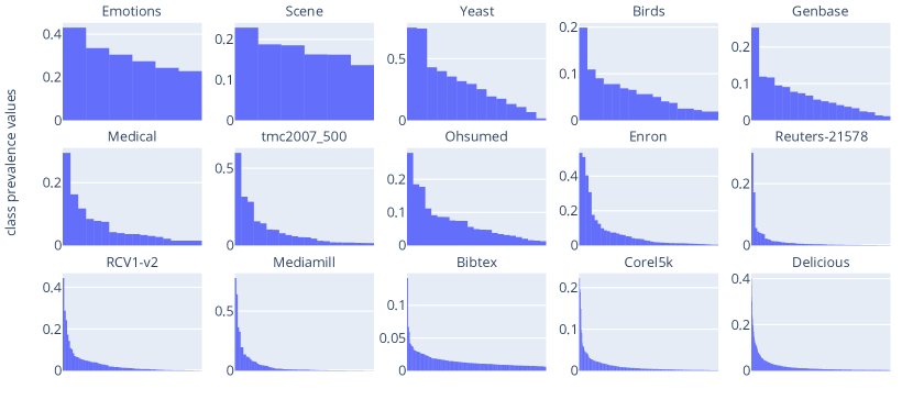
Figure 3: Histograms of class prevalence values, one per dataset, sorted from highly populated datasets to lowly populated ones; values on the $x$ axis indicate intervals $[\alpha_{k},\beta_{k}]$ of class prevalence values, while values on the $y$ axis indicate the fraction of classes in the dataset that have prevalence values in the $[\alpha_{k},\beta_{k}]$ interval.

We set the parameters of the ML-APP for generating test samples (see Section 4) as follows. We fix the sample size to $k=100$ in all cases. We set the grid of prevalence values to $\mathbf{g}=\{0.00,0.01,\ldots,0.99,1.00\}$ in all cases but for dataset Delicious, since in this latter the number of combinations thus generated would be intractable, given that this is dataset with no fewer than 983 classes; for Delicious we use the coarser-grained grid $\mathbf{g}=\{0.00,0.05,\ldots,0.95,1.00\}$. We set $m$ (the number of samples to be drawn for each prevalence value) independently for each dataset, to the smallest number that yields more than 10,000 test samples ($m$ ranges from 1 in Delicious to 40 in Birds).

We break down the results into three groups, each corresponding to a different amount of shift. The rationale behind this choice is to allow for a more meaningful analysis of the quantifiers’ performance, since the APP (and, by extension, the ML-APP) has often been the subject of criticism for generating samples exhibiting degrees of shift that are judged unrealistic and unlikely to occur in real cases [12, 72]. We instead believe that general-purpose quantification methods should be tested in widely varying situations, from low-shift to high-shift ones, and we thus prefer to test all such scenarios, but split the corresponding results into groups characterized by of more or less homogeneous amounts of shift.

More specifically, for each test sample generated via the ML-APP, we compute its prior probability shift with respect to the training set in terms of $\operatorname{AE}$ between the vectors of training and test class prevalence values. We then bring together all the resulting shift values and split the range of such values in three equally-sized intervals (that we dub low shift, mid shift, and high shift). The accuracy values we report are thus not averages across the same number of experiments, since the ML-APP often tends to generate more samples in the low-shift region than samples in the mid-shift region and (above all) in the high-shift region. The number of samples, as well as the distribution of shift values, depends on each dataset.

Figure 4 shows the distributions of shift values that the ML-APP generates (blue) along with the distributions of shift values that we would obtain via uniform sampling (red). Note that the ML-APP succeeds in generating larger amounts of shift, and that most of the samples generated via uniform sampling would fall within what we call the “low shift” region.

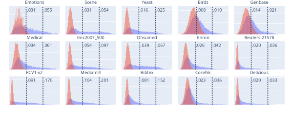
Figure 4: Shifts generated via the proposed ML-APP (blue) and via uniform sampling (blue), as computed in terms of $\operatorname{AE}$ between the training set and the test samples.

6.3 Testing Instances of the Four Types of Multi-Label Quantification Methods

The goal of this section is to provide an answer to the question: “Which among the four groups of multi-label quantification methods tends to perform best?”

To this aim, we choose one representative instance from each group, and carry out the experiments using all the datasets. We perform this choice by combining the following components:

• As the binary classification method, we choose logistic regression (LR), and use the implementation of it available from scikit-learn. We consider LR a good choice, given that it is a probabilistic classifier that already provides fairly well calibrated posterior probabilities (which is of fundamental importance in PCC, PACC, and SLD), and given that, as indicated by previously reported results [73], it tends to perform well. A set of LR classifiers are used when testing the binary relevance (BR) method described in Section 3.2.2.

• As the multi-label classification method, we adopt stacked generalization [58] (SG – see Section 3.2.3). We use our own implementation (since the implementation of stacked generalization available from scikit-learn only caters for the single-label case), that relies on 5-fold cross-validation to generate the intermediate representations (in the form of posterior probabilities) given as input to the meta-learner, concatenated with the original input features. The base members of the ensemble consist of binary logistic regression classifiers as implemented in scikit-learn.

• As the binary aggregation method Q, we experiment with all the methods covered in Section 5.1, i.e., CC, PCC, ACC, PACC, SLD. For all these methods we use the implementations made available in the QuaPy open-source library [73].

• As the multi-label aggregation method, we use the regressor-based strategy for quantification (that we dub RQ) described in Section 5.2.1. We implement this method as part of the QuaPy framework. For training the base quantifier $q$ we experiment again with all the methods covered in Section 5.1, i.e., CC, PCC, ACC, PACC, SLD, while as the internal regressor which receives its input from the base quantifier $q$ we use linear support vector regression (SVR), for which we use the scikit-learn implementation. As the held-out validation set $L_{R}$ needed for training the regressor we use a set consisting of 40% of the training datapoints, chosen via iterative stratification [68, 67] as implemented in scikit-multilearn. We call this aggregation method SVR-RQ.

The methods we use in this experiment thus amount to the combinations illustrated in Table 2.

Table 2: Methods we use as instances of the four types of methods illustrated in Figure 1.

Type	Classification	Aggregation
BC+BA	LR	Q$\in${CC,PCC,ACC,PACC,SLD}
MLC+BA	SG	Q$\in${CC,PCC,ACC,PACC,SLD}
BC+MLA	LR	Q$\in${CC,PCC,ACC,PACC,SLD} + SVR-RQ
MLC+MLA	SG	Q$\in${CC,PCC,ACC,PACC,SLD} + SVR-RQ

Following [65], we perform model selection by using, as the loss function to minimize, a quantification-oriented error measure (and not a classification-oriented one), and by adopting the same protocol used for the evaluation of our quantifiers. That is, model selection is carried out by first splitting the training set $L$ into two disjoint sets, i.e., (a) a proper training set $L_{\operatorname{tr}}$ and (b) a held-out validation set $L_{\operatorname{va}}$ consisting of 40% of the labelled datapoints. For splitting the training set, we again rely on the iterative stratification routine of scikit-multilearn (see Footnote 2). We use $L_{\operatorname{tr}}$ to train the quantifiers with different combinations of hyperparameters, while from $L_{\operatorname{va}}$ we extract, via the ML-APP, validation samples on which we assess, via $\operatorname{AE}$ (the same measure we use in the evaluation phase), the quality of the hyperparameter combinations. We explore the hyperparameters via grid-search optimization, and use the best configuration to retrain the quantifier on the entire training set $L$ after model selection. During the model selection phase, for the ML-APP we use the same parameters $k$ and $\mathbf{g}$ that we use in the test phase, but we reduce the number of repetitions $m$ to 5 in the datasets with fewer than 90 classes, and to 1 in the other datasets, in order to keep the computational burden under reasonable bounds.

The hyperparameters we explore for LR include $C$, the inverse of the regularization strength, in the range $\{10^{-1},10^{0},10^{1},10^{2},10^{3}\}$, and ClassWeight, which takes values in Balanced (which reweights the importance of the examples so as to equate the overall contribution of each class) or None (which gives the same weight to all datapoints, irrespectively of the prevalence of the class they belong to). In cases in which the class-specific classifiers are independent of each other (i.e., for methods belonging to the BC+BA and BC+MLA types) we optimize the hyperparameters independently for each class. For SG, we only optimize the hyperparameters of the meta-classifier, leaving the hyperparameters of the base members to their default values. In particular, we explore the parameters $C$ and ClassWeight as before, plus the hyperparameter Normalize, which takes values in True (which has the effect of standardizing the inputs of the meta-classifier so that every dimension has zero mean and unit variance) and False (which does not standardize the inputs). For RQ we only explore the regularization hyperparameter $C$ in the range $\{10^{-1},10^{0},10^{1},10^{2},10^{3}\}$. Note that the base quantifiers (i.e., CC, PCC, ACC, PACC, SLD) have no specific internal hyperparameters to be tuned.

The results we have obtained for the different choices of the base quantifier are reported in Table 3 for CC, Table 4 for PCC, Table 5 for ACC, Table 6 for PACC, and Table 7 for SLD. The results clearly show (see especially the last two rows of each table) that there is an ordering BC+BA $\prec$ MLC+BA $\prec$ BC+MLA $\prec$ MLC+MLA, in which $\prec$ means “performs worse than”, which holds, independently of the base quantifier of choice, in almost all cases. The same experiments also indicate that there is a substantial improvement in performance that derives from simply replacing the binary classifiers with one multi-label classifier (moving from BC+BA to MLC+BA or from BC+MLA to MLC+MLA), i.e., from bringing to bear the class-class correlations at the classification stage, and that there is an equally substantial improvement when binary aggregation is replaced by multi-label aggregation (switching from BC+BA to BC+MLA or from MLC+BA to MLC+MLA), i.e., when the class-class correlations are exploited at the aggregation stage. What also emerges from these results is that, consistently with the above observations, the best-performing group of methods is MLC+MLA, i.e., methods that explicitly take class dependencies into account both at the classification stage and at the aggregation stage.

Note that methods that learn from the stochastic correlations among the classes perform much better than methods that do not, even in the low shift regime. Overall, the best-performing method on average is MLC+MLA when equipped with PCC as the base quantifier.

The reader might wonder why we do not use as a baseline the system presented in the only paper in the literature that tackles multi-label quantification, i.e., [32]. There are several reasons for this: (a) the authors do not make the code available; (b) the method is, as already discussed in Section 3.1, computationally expensive, and as a result the authors test it on a single dataset whose codeframe consists of 16 classes only; using this method on our 15 datasets, whose codeframes count up to 983 classes, and 125 classes on average, would be prohibitive; (c) the method is essentially a calibration strategy for binary classification, which means that it falls in the group of “naive” BC+BA methods since it does not tackle at all, as already mentioned in Section 3.1, the multi-label nature of the MLQ problem.

Table 3: Values of $\operatorname{AE}$ obtained in our experiments for different amounts of shift using CC as the base quantifier. The number of test samples generated for each dataset exceeds 10,000, though there is a variable number of samples allocated in each region of shift. Boldface indicates the best method for a given dataset and shift region. Superscripts ${\dagger}$ and ${\ddagger}$ denote the methods (if any) whose scores are not statistically significantly different from the best one according to a Wilcoxon signed-rank test at different confidence levels: symbol ${\dagger}$ indicates 0.001 $<$ $p$-value $<$ 0.05 while symbol ${\ddagger}$ indicates 0.05 $\leq$ $p$-value. For ease of readability, for each pair {dataset, shift} we colour-code cells via intense green for the best result, intense red for the worst result, and an interpolated tone for the scores in-between.

	low shift				mid shift				high shift
	BC+BA	MLC+BA	BC+MLA	MLC+MLA0	BC+BA	MLC+BA	BC+MLA	MLC+MLA0	BC+BA	MLC+BA	BC+MLA	MLC+MLA0
Emotions	.0749	.0626	.0478	.0644${}^{\phantom{{\ddagger}}}$	.0838	.0776	.0598${}^{\phantom{{\ddagger}}}$	.0848	.0967	.0899	.0616${}^{\phantom{{\ddagger}}}$	.1039${}^{\phantom{{\ddagger}}}$
Scene	.0754	.0558	.0458	.0349${}^{\phantom{{\ddagger}}}$	.0908	.0759	.0553${}^{\phantom{{\ddagger}}}$	.0508	.1110	.0966	.0609${}^{\phantom{{\ddagger}}}$	.0668${}^{\phantom{{\ddagger}}}$
Yeast	.1481	.1119	.0511	.0516${}^{{\dagger}\phantom{{\dagger}}}$	.1644	.1397	.0879${}^{\phantom{{\ddagger}}}$	.0958	.1919	.1754	.1272${}^{\phantom{{\ddagger}}}$	.1403${}^{\phantom{{\ddagger}}}$
Birds	.0229	.0243	.0191	.0202${}^{\phantom{{\ddagger}}}$	.0258	.0276	.0255${}^{\phantom{{\ddagger}}}$	.0264	.0293	.0331	.0371${}^{\phantom{{\ddagger}}}$	.0357${}^{\phantom{{\ddagger}}}$
Genbase	.0003	.0006	.0016	.0007${}^{\phantom{{\ddagger}}}$	.0003	.0006	.0018${}^{\phantom{{\ddagger}}}$	.0007	.0003	.0005	.0017${}^{\phantom{{\ddagger}}}$	.0006${}^{\phantom{{\ddagger}}}$
Medical	.0182	.0121	.0175	.0121${}^{\phantom{{\ddagger}}}$	.0183	.0130	.0206${}^{\phantom{{\ddagger}}}$	.0130	.0174	.0141	.0230${}^{\phantom{{\ddagger}}}$	.0141${}^{\phantom{{\ddagger}}}$
tmc2007_500	.0700	.0333	.0222	.0214${}^{\phantom{{\ddagger}}}$	.0758	.0464	.0313${}^{\phantom{{\ddagger}}}$	.0278	.0651	.0468	.0333${}^{\phantom{{\ddagger}}}$	.0320${}^{\phantom{{\ddagger}}}$
Ohsumed	.0338	.0184	.0198	.0176${}^{\phantom{{\ddagger}}}$	.0395	.0252	.0246${}^{\phantom{{\ddagger}}}$	.0236	.0457	.0303	.0270${}^{\phantom{{\ddagger}}}$	.0272‡
Enron	.0239	.0207	.0172	.0198${}^{\phantom{{\ddagger}}}$	.0274	.0247	.0228${}^{\phantom{{\ddagger}}}$	.0245	.0280	.0253	.0254‡	.0265${}^{\phantom{{\ddagger}}}$
Reuters-21578	.0067	.0035	.0055	.0036${}^{\phantom{{\ddagger}}}$	.0120	.0056	.0081${}^{\phantom{{\ddagger}}}$	.0058	.0291	.0071	.0113${}^{\phantom{{\ddagger}}}$	.0075${}^{\phantom{{\ddagger}}}$
RCV1-v2	.0198	.0081	.0101	.0083${}^{\phantom{{\ddagger}}}$	.0251	.0118	.0162${}^{\phantom{{\ddagger}}}$	.0122	.0360	.0176	.0240${}^{\phantom{{\ddagger}}}$	.0192${}^{\phantom{{\ddagger}}}$
Mediamill	.1390	.0236	.0159	.0155${}^{\phantom{{\ddagger}}}$	.1488	.0341	.0252${}^{\phantom{{\ddagger}}}$	.0247	.1690	.0476	.0322${}^{\phantom{{\ddagger}}}$	.0310${}^{\phantom{{\ddagger}}}$
Bibtex	.0137	.0097	.0093	.0096${}^{\phantom{{\ddagger}}}$	.0150	.0111	.0117${}^{\phantom{{\ddagger}}}$	.0113	.0177	.0120	.0131${}^{\phantom{{\ddagger}}}$	.0124${}^{\phantom{{\ddagger}}}$
Corel5k	.0357	.0093	.0082	.0082${}^{\phantom{{\ddagger}}}$	.0363	.0097	.0087${}^{\phantom{{\ddagger}}}$	.0092	.0371	.0100	.0099${}^{\phantom{{\ddagger}}}$	.0095${}^{\phantom{{\ddagger}}}$
Delicious	.1037	.0116	.0096	.0094${}^{\phantom{{\ddagger}}}$	.1036	.0134	.0113‡	.0112	.0904	.0128	.0109${}^{\phantom{{\ddagger}}}$	.0110‡
Average	.0492	.0237	.0180	.0177${}^{\phantom{{\ddagger}}}$	.0555	.0358	.0288${}^{\phantom{{\ddagger}}}$	.0295	.0757	.0576	.0433${}^{\phantom{{\ddagger}}}$	.0483${}^{\phantom{{\ddagger}}}$
Rank Average	3.7	2.5	2.0	1.8	3.5	2.4	2.1	1.9	3.5	2.1	2.3	2.1

Table 4: Values of $\operatorname{AE}$ obtained in our experiments for different amounts of shift using PCC as the base quantifier. Notational conventions are as in Table 3.

	low shift				mid shift				high shift
	BC+BA	MLC+BA	BC+MLA	MLC+MLA0	BC+BA	MLC+BA	BC+MLA	MLC+MLA0	BC+BA	MLC+BA	BC+MLA	MLC+MLA0
Emotions	.0418	.0420	.0586	.0474	.0685	.0654${}^{\phantom{{\ddagger}}}$	.0720	.0564${}^{\phantom{{\ddagger}}}$	.0923	.0857	.0951	.0664
Scene	.0842	.0362	.0384	.0323	.1140	.0827${}^{\phantom{{\ddagger}}}$	.0459	.0445${}^{\phantom{{\ddagger}}}$	.1427	.1221	.0499	.0589
Yeast	.1756	.0444	.0480	.0472	.1900	.0992${}^{\phantom{{\ddagger}}}$	.0913	.0845${}^{\phantom{{\ddagger}}}$	.2206	.1549	.1361	.1226
Birds	.0286	.0208	.0181	.0213	.0328	.0246${}^{\phantom{{\ddagger}}}$	.0243	.0288${}^{\phantom{{\ddagger}}}$	.0440	.0321	.0351	.0404
Genbase	.0011	.0005	.0022	.0007	.0011	.0005${}^{\phantom{{\ddagger}}}$	.0025	.0007${}^{\phantom{{\ddagger}}}$	.0010	.0005	.0023	.0006
Medical	.0127	.0138	.0191	.0120	.0146	.0156${}^{\phantom{{\ddagger}}}$	.0279	.0136${}^{\phantom{{\ddagger}}}$	.0169	.0183	.0351	.0160
tmc2007_500	.1108	.0193	.0213	.0186	.1154	.0331${}^{\phantom{{\ddagger}}}$	.0292	.0231${}^{\phantom{{\ddagger}}}$	.1008	.0399	.0321	.0255
Ohsumed	.1004	.0177	.0183	.0168	.1087	.0262${}^{\phantom{{\ddagger}}}$	.0209	.0238${}^{\phantom{{\ddagger}}}$	.1177	.0321	.0215	.0284
Enron	.0347	.0161	.0169	.0185	.0397	.0235${}^{\phantom{{\ddagger}}}$	.0227	.0228†	.0439	.0287	.0253	.0246
Reuters-21578	.0167	.0036	.0049	.0037	.0243	.0059${}^{\phantom{{\ddagger}}}$	.0070	.0060${}^{\phantom{{\ddagger}}}$	.0370	.0075	.0088	.0078
RCV1-v2	.0456	.0084	.0093	.0084	.0533	.0129†	.0146	.0128${}^{\phantom{{\ddagger}}}$	.0654	.0198	.0215	.0201
Mediamill	.1697	.0154	.0157	.0148	.1736	.0285${}^{\phantom{{\ddagger}}}$	.0251	.0231${}^{\phantom{{\ddagger}}}$	.1806	.0401	.0322	.0285
Bibtex	.0354	.0091	.0092	.0093	.0374	.0126${}^{\phantom{{\ddagger}}}$	.0116	.0120${}^{\phantom{{\ddagger}}}$	.0423	.0152	.0129	.0142
Corel5k	.0582	.0077	.0075	.0066	.0585	.0083${}^{\phantom{{\ddagger}}}$	.0082	.0074${}^{\phantom{{\ddagger}}}$	.0594	.0089	.0087	.0085
Delicious	.1420	.0088	.0093	.0084	.1417	.0117${}^{\phantom{{\ddagger}}}$	.0109	.0098${}^{\phantom{{\ddagger}}}$	.1238	.0119	.0104	.0092
Average	.0677	.0158	.0177	.0160	.0761	.0312${}^{\phantom{{\ddagger}}}$	.0288	.0261${}^{\phantom{{\ddagger}}}$	.1012	.0602	.0452	.0414
Rank Average	3.6	1.7	2.9	1.8	3.7	2.5	2.3	1.5	3.7	2.4	2.3	1.5

Table 5: Values of $\operatorname{AE}$ obtained in our experiments for different amounts of shift using ACC as the base quantifier. Notational conventions are as in Table 3.

	low shift				mid shift				high shift
	BC+BA	MLC+BA	BC+MLA	MLC+MLA0	BC+BA	MLC+BA	BC+MLA	MLC+MLA0	BC+BA	MLC+BA	BC+MLA	MLC+MLA0
Emotions	.1060	.1279	.0626	.0440	.1367	.1487	.0732${}^{\phantom{{\ddagger}}}$	.0551${}^{\phantom{{\ddagger}}}$	.1608	.1602${}^{\phantom{{\ddagger}}}$	.1125	.0750${}^{\phantom{{\ddagger}}}$
Scene	.0537	.0436	.0456	.0361	.0626	.0601	.0512${}^{\phantom{{\ddagger}}}$	.0513‡	.0615	.0603‡	.0596	.0711${}^{\phantom{{\ddagger}}}$
Yeast	.1937	.1765	.0506	.0531	.2164	.2191	.0896${}^{\phantom{{\ddagger}}}$	.0957${}^{\phantom{{\ddagger}}}$	.2301	.2620${}^{\phantom{{\ddagger}}}$	.1204	.1480${}^{\phantom{{\ddagger}}}$
Birds	.1542	.1353	.0233	.0278	.1526	.1384	.0286${}^{\phantom{{\ddagger}}}$	.0307${}^{\phantom{{\ddagger}}}$	.1547	.1472${}^{\phantom{{\ddagger}}}$	.0359	.0391${}^{\phantom{{\ddagger}}}$
Genbase	.0014	.0007	.0036	.0006	.0014	.0007	.0039${}^{\phantom{{\ddagger}}}$	.0007‡	.0013	.0006‡	.0037	.0006${}^{\phantom{{\ddagger}}}$
Medical	.0212	.0307	.0187	.0183	.0189	.0329	.0259${}^{\phantom{{\ddagger}}}$	.0248${}^{\phantom{{\ddagger}}}$	.0153	.0329${}^{\phantom{{\ddagger}}}$	.0311	.0294${}^{\phantom{{\ddagger}}}$
tmc2007_500	.0366	.0365	.0220	.0222	.0612	.0581	.0302${}^{\phantom{{\ddagger}}}$	.0278${}^{\phantom{{\ddagger}}}$	.0647	.0591${}^{\phantom{{\ddagger}}}$	.0339	.0315${}^{\phantom{{\ddagger}}}$
Ohsumed	.0253	.0241	.0198	.0180	.0320	.0292	.0228†	.0226${}^{\phantom{{\ddagger}}}$	.0407	.0337${}^{\phantom{{\ddagger}}}$	.0239	.0263${}^{\phantom{{\ddagger}}}$
Enron	.1810	.0935	.0187	.0207	.1882	.0982	.0243${}^{\phantom{{\ddagger}}}$	.0272${}^{\phantom{{\ddagger}}}$	.1853	.1043${}^{\phantom{{\ddagger}}}$	.0269	.0339${}^{\phantom{{\ddagger}}}$
Reuters-21578	.0307	.0074	.0055	.0065	.0336	.0121	.0078${}^{\phantom{{\ddagger}}}$	.0096${}^{\phantom{{\ddagger}}}$	.0421	.0254${}^{\phantom{{\ddagger}}}$	.0104	.0123${}^{\phantom{{\ddagger}}}$
RCV1-v2	.0124	.0217	.0099	.0106	.0189	.0259	.0158${}^{\phantom{{\ddagger}}}$	.0167${}^{\phantom{{\ddagger}}}$	.0287	.0335${}^{\phantom{{\ddagger}}}$	.0246	.0269${}^{\phantom{{\ddagger}}}$
Mediamill	.0539	.0425	.0164	.0163	.0976	.0539	.0246${}^{\phantom{{\ddagger}}}$	.0274${}^{\phantom{{\ddagger}}}$	.1467	.0647${}^{\phantom{{\ddagger}}}$	.0316	.0374${}^{\phantom{{\ddagger}}}$
Bibtex	.0692	.0816	.0102	.0107	.0734	.0858	.0125${}^{\phantom{{\ddagger}}}$	.0152${}^{\phantom{{\ddagger}}}$	.0861	.0903${}^{\phantom{{\ddagger}}}$	.0146	.0196${}^{\phantom{{\ddagger}}}$
Corel5k	.1515	.0173	.0081	.0062	.1537	.0158	.0089${}^{\phantom{{\ddagger}}}$	.0076${}^{\phantom{{\ddagger}}}$	.1509	.0149${}^{\phantom{{\ddagger}}}$	.0099	.0094${}^{\phantom{{\ddagger}}}$
Delicious	.0846	.0528	.0097	.0093	.1000	.0531	.0111${}^{\phantom{{\ddagger}}}$	.0110${}^{\phantom{{\ddagger}}}$	.1016	.0492${}^{\phantom{{\ddagger}}}$	.0106	.0109†
Average	.0750	.0558	.0193	.0182	.0841	.0716	.0302${}^{\phantom{{\ddagger}}}$	.0296${}^{\phantom{{\ddagger}}}$	.0901	.0808${}^{\phantom{{\ddagger}}}$	.0482	.0495${}^{\phantom{{\ddagger}}}$
Rank Average	3.7	3.1	1.7	1.5	3.5	3.2	1.7	1.7	3.5	3.1	1.5	1.9

Table 6: Values of $\operatorname{AE}$ obtained in our experiments for different amounts of shift using PACC as the base quantifier. Notational conventions are as in Table 3.

	low shift				mid shift				high shift
	BC+BA	MLC+BA	BC+MLA	MLC+MLA0	BC+BA	MLC+BA	BC+MLA	MLC+MLA0	BC+BA	MLC+BA	BC+MLA	MLC+MLA0
Emotions	.1326	.0715	.0509${}^{\phantom{{\ddagger}}}$	.0516	.1451	.1049	.0659${}^{\phantom{{\ddagger}}}$	.0633	.1578	.1485${}^{\phantom{{\ddagger}}}$	.1101${}^{\phantom{{\ddagger}}}$	.0872${}^{\phantom{{\ddagger}}}$
Scene	.0508	.0379	.0391${}^{\phantom{{\ddagger}}}$	.0310	.0697	.0498	.0433${}^{\phantom{{\ddagger}}}$	.0441	.0757	.0499‡	.0496${}^{\phantom{{\ddagger}}}$	.0645${}^{\phantom{{\ddagger}}}$
Yeast	.1654	.1436	.0489${}^{\phantom{{\ddagger}}}$	.0494	.2122	.1803	.0878${}^{\phantom{{\ddagger}}}$	.0837	.2474	.2053${}^{\phantom{{\ddagger}}}$	.1316${}^{\phantom{{\ddagger}}}$	.1264${}^{\phantom{{\ddagger}}}$
Birds	.1253	.1290	.0191${}^{\phantom{{\ddagger}}}$	.0227	.1243	.1286	.0244${}^{\phantom{{\ddagger}}}$	.0282	.1250	.1173${}^{\phantom{{\ddagger}}}$	.0377${}^{\phantom{{\ddagger}}}$	.0434${}^{\phantom{{\ddagger}}}$
Genbase	.0018	.0010	.0041${}^{\phantom{{\ddagger}}}$	.0016	.0018	.0010	.0043${}^{\phantom{{\ddagger}}}$	.0015	.0018	.0010${}^{\phantom{{\ddagger}}}$	.0041${}^{\phantom{{\ddagger}}}$	.0015${}^{\phantom{{\ddagger}}}$
Medical	.0395	.0272	.0169${}^{\phantom{{\ddagger}}}$	.0161	.0477	.0276	.0204${}^{\phantom{{\ddagger}}}$	.0222	.0484	.0267${}^{\phantom{{\ddagger}}}$	.0286†	.0286${}^{\phantom{{\ddagger}}}$
tmc2007_500	.0351	.0285	.0213${}^{\phantom{{\ddagger}}}$	.0192	.0617	.0454	.0281${}^{\phantom{{\ddagger}}}$	.0236	.0619	.0466${}^{\phantom{{\ddagger}}}$	.0320${}^{\phantom{{\ddagger}}}$	.0275${}^{\phantom{{\ddagger}}}$
Ohsumed	.0239	.0221	.0189${}^{\phantom{{\ddagger}}}$	.0179	.0345	.0285	.0205${}^{\phantom{{\ddagger}}}$	.0234	.0452	.0332${}^{\phantom{{\ddagger}}}$	.0216${}^{\phantom{{\ddagger}}}$	.0278${}^{\phantom{{\ddagger}}}$
Enron	.1433	.1429	.0198${}^{\phantom{{\ddagger}}}$	.0201	.1618	.1539	.0243†	.0239	.1504	.1693${}^{\phantom{{\ddagger}}}$	.0275${}^{\phantom{{\ddagger}}}$	.0253${}^{\phantom{{\ddagger}}}$
Reuters-21578	.0086	.0465	.0053${}^{\phantom{{\ddagger}}}$	.0054	.0311	.0519	.0076${}^{\phantom{{\ddagger}}}$	.0087	.0643	.0619${}^{\phantom{{\ddagger}}}$	.0113${}^{\phantom{{\ddagger}}}$	.0117${}^{\phantom{{\ddagger}}}$
RCV1-v2	.0173	.0130	.0098${}^{\phantom{{\ddagger}}}$	.0093	.0334	.0228	.0159${}^{\phantom{{\ddagger}}}$	.0148	.0505	.0342${}^{\phantom{{\ddagger}}}$	.0243${}^{\phantom{{\ddagger}}}$	.0232${}^{\phantom{{\ddagger}}}$
Mediamill	.0482	.0466	.0158†	.0158	.0941	.0779	.0237${}^{\phantom{{\ddagger}}}$	.0235	.1387	.1076${}^{\phantom{{\ddagger}}}$	.0299${}^{\phantom{{\ddagger}}}$	.0300‡
Bibtex	.0320	.0218	.0099${}^{\phantom{{\ddagger}}}$	.0100	.0459	.0387	.0121${}^{\phantom{{\ddagger}}}$	.0133	.0684	.0662${}^{\phantom{{\ddagger}}}$	.0140${}^{\phantom{{\ddagger}}}$	.0161${}^{\phantom{{\ddagger}}}$
Corel5k	.1519	.1014	.0107${}^{\phantom{{\ddagger}}}$	.0111	.1559	.1087	.0112‡	.0112	.1711	.1221${}^{\phantom{{\ddagger}}}$	.0120${}^{\phantom{{\ddagger}}}$	.0116${}^{\phantom{{\ddagger}}}$
Delicious	.0594	.0480	.0094${}^{\phantom{{\ddagger}}}$	.0092	.0837	.0828	.0107${}^{\phantom{{\ddagger}}}$	.0105	.0871	.0914${}^{\phantom{{\ddagger}}}$	.0101†	.0099${}^{\phantom{{\ddagger}}}$
Average	.0646	.0561	.0181${}^{\phantom{{\ddagger}}}$	.0175	.0823	.0701	.0279${}^{\phantom{{\ddagger}}}$	.0276	.0958	.0782${}^{\phantom{{\ddagger}}}$	.0463${}^{\phantom{{\ddagger}}}$	.0467†
Rank Average	3.8	2.9	1.7	1.5	3.8	3.0	1.7	1.5	3.8	2.8	1.7	1.7

Table 7: Values of $\operatorname{AE}$ obtained in our experiments for different amounts of shift using SLD as the base quantifier. Notational conventions are as in Table 3.

	low shift				mid shift				high shift
	BC+BA	MLC+BA	BC+MLA	MLC+MLA0	BC+BA	MLC+BA	BC+MLA	MLC+MLA0	BC+BA	MLC+BA	BC+MLA	MLC+MLA0
Emotions	.2169	.0549	.0710${}^{\phantom{{\ddagger}}}$	.0509	.2189	.0719${}^{\phantom{{\ddagger}}}$	.0791	.0652	.2088	.0890${}^{\phantom{{\ddagger}}}$	.0822${}^{\phantom{{\ddagger}}}$	.0717${}^{\phantom{{\ddagger}}}$
Scene	.0407	.0433	.0337${}^{\phantom{{\ddagger}}}$	.0424	.0467	.0753${}^{\phantom{{\ddagger}}}$	.0497	.0709	.0487	.1012${}^{\phantom{{\ddagger}}}$	.0628${}^{\phantom{{\ddagger}}}$	.0881${}^{\phantom{{\ddagger}}}$
Yeast	.2557	.0948	.0511${}^{\phantom{{\ddagger}}}$	.0500	.2607	.1192${}^{\phantom{{\ddagger}}}$	.0889	.0827	.2939	.1438${}^{\phantom{{\ddagger}}}$	.1362${}^{\phantom{{\ddagger}}}$	.1171${}^{\phantom{{\ddagger}}}$
Birds	.0759	.0284	.0196${}^{\phantom{{\ddagger}}}$	.0281	.0819	.0312${}^{\phantom{{\ddagger}}}$	.0255	.0312	.1089	.0355†	.0358†	.0351${}^{\phantom{{\ddagger}}}$
Genbase	.0011	.0004	.0039${}^{\phantom{{\ddagger}}}$	.0005	.0011	.0003${}^{\phantom{{\ddagger}}}$	.0042	.0005	.0010	.0003${}^{\phantom{{\ddagger}}}$	.0041${}^{\phantom{{\ddagger}}}$	.0005${}^{\phantom{{\ddagger}}}$
Medical	.0233	.0133	.0190${}^{\phantom{{\ddagger}}}$	.0129	.0211	.0135${}^{\phantom{{\ddagger}}}$	.0263	.0131	.0189	.0133${}^{\phantom{{\ddagger}}}$	.0312${}^{\phantom{{\ddagger}}}$	.0132${}^{\phantom{{\ddagger}}}$
tmc2007_500	.0384	.0248	.0202${}^{\phantom{{\ddagger}}}$	.0187	.0526	.0407${}^{\phantom{{\ddagger}}}$	.0285	.0230	.0546	.0432${}^{\phantom{{\ddagger}}}$	.0330${}^{\phantom{{\ddagger}}}$	.0228${}^{\phantom{{\ddagger}}}$
Ohsumed	.0294	.0186	.0173${}^{\phantom{{\ddagger}}}$	.0185	.0316	.0232${}^{\phantom{{\ddagger}}}$	.0189	.0232	.0321	.0250${}^{\phantom{{\ddagger}}}$	.0200${}^{\phantom{{\ddagger}}}$	.0250${}^{\phantom{{\ddagger}}}$
Enron	.0918	.0208	.0183${}^{\phantom{{\ddagger}}}$	.0182	.0915	.0253${}^{\phantom{{\ddagger}}}$	.0238	.0243	.0838	.0261†	.0258${}^{\phantom{{\ddagger}}}$	.0263†
Reuters-21578	.0050	.0039	.0048${}^{\phantom{{\ddagger}}}$	.0040	.0177	.0055${}^{\phantom{{\ddagger}}}$	.0079	.0056	.0956	.0088${}^{\phantom{{\ddagger}}}$	.0112${}^{\phantom{{\ddagger}}}$	.0083${}^{\phantom{{\ddagger}}}$
RCV1-v2	.0109	.0089	.0090†	.0088	.0185	.0110${}^{\phantom{{\ddagger}}}$	.0151	.0113	.0340	.0173${}^{\phantom{{\ddagger}}}$	.0261${}^{\phantom{{\ddagger}}}$	.0178${}^{\phantom{{\ddagger}}}$
Mediamill	.2040	.0237	.0151${}^{\phantom{{\ddagger}}}$	.0145	.2204	.0444${}^{\phantom{{\ddagger}}}$	.0238	.0223	.2481	.0695${}^{\phantom{{\ddagger}}}$	.0308${}^{\phantom{{\ddagger}}}$	.0282${}^{\phantom{{\ddagger}}}$
Bibtex	.0819	.0103	.0100${}^{\phantom{{\ddagger}}}$	.0101	.0919	.0116†	.0137	.0116	.1084	.0128‡	.0183${}^{\phantom{{\ddagger}}}$	.0127${}^{\phantom{{\ddagger}}}$
Corel5k	.1043	.0098	.0140${}^{\phantom{{\ddagger}}}$	.0178	.1041	.0101${}^{\phantom{{\ddagger}}}$	.0145	.0177	.1043	.0099${}^{\phantom{{\ddagger}}}$	.0155${}^{\phantom{{\ddagger}}}$	.0182${}^{\phantom{{\ddagger}}}$
Delicious	.1406	.0137	.0095${}^{\phantom{{\ddagger}}}$	.0100	.1511	.0155${}^{\phantom{{\ddagger}}}$	.0110	.0114	.1345	.0155${}^{\phantom{{\ddagger}}}$	.0106${}^{\phantom{{\ddagger}}}$	.0108‡
Average	.0842	.0219	.0189${}^{\phantom{{\ddagger}}}$	.0182	.0862	.0346${}^{\phantom{{\ddagger}}}$	.0296	.0285	.0957	.0562${}^{\phantom{{\ddagger}}}$	.0466${}^{\phantom{{\ddagger}}}$	.0459${}^{\phantom{{\ddagger}}}$
Rank Average	3.8	2.5	2.1	1.7	3.7	2.3	2.3	1.8	3.7	2.3	2.3	1.7

In the following sections, we turn to explore other instances of methods of the four groups in Figure 1 beyond the ones we choose in Table 2.

6.4 Testing Additional Instances of MLC+BA

In this section we explore other methods relying on different multi-label classifiers, with the aim of studying the extent to which the results we have obtained in the previous experiments depend on the choice of the classifier being employed. To this aim, we focus on the MLC+BA group of methods, so that the aggregation stage plays only a minimal role. As a quantification method we adopt PCC, since this is the base quantifier that has yielded the best performance overall in the experiments of Section 6.3. The methods we study here thus consist of genuinely multi-label classifiers that generate posterior probabilities, where the latter are then aggregated by computing the expected value for each class. The aim of this experiment is not to provide an exhaustive evaluation of existing multi-label classifiers, but rather to study other MLC+BA configurations in action, and hopefully pinpoint interesting performance trends.

With this in mind, we choose some representative instances from the main families of multi-label classifiers discussed in Section 3. The multi-label classifiers we consider here include (a) multi-label versions of KNN (ML-knn), decision trees (DT), and random forests (RF) as representatives of the family of “algorithm adaptation” methods (Section 3.2.2); (b) classifier chains (CChains) as representative of the family of “problem transformation” methods (Section 3.2.1); and (c) CLEMS and label space clustering (LSC) as representatives of the family of “ensemble” methods (Section 3.2.3). For the sake of comparison, we also include stacked generalization (SG – another ensemble method and the multi-label classifier we choose for the experiments of Section 6.3), and BC+BA (with PCC as the binary quantifier and LR as the binary classifier) acting as a lower bound baseline. Values for SG and BC+BA are taken from Table 4. We carry out model selection by optimizing the hyperparameters listed succinctly in Table 8. The results we have obtained are presented in Table 9.

Table 8: Hyperparameters we explore during model selection for different multi-label classifiers.

Classifier	Hyperparameter	Description	Values
ML-knn0	$k$	number of neighbours	{1, 3, 5, 7, 9}
	$s$	smoothing factor	{0.5, 0.7, 1}
DT	Criterion	split function	{Gini, Entropy}
RF	N_estimators	number of trees	{10, 100, 200}
CChains	$C$	inverse regularization strength	$\{10^{-1},\ldots,10^{2},10^{3}\}$
	ClassWeight	weights associated with classes	{None, Balanced}
CLEMS	N_estimators	number of trees	{10, 20, 50}
	$k$	number of neighbours	{1, 3, 5, 7, 9}
	$s$	smoothing factor	{0.5, 0.7, 1}
LSC	N_clusters	number of clusters	{2, 3, 5, 10, 50}
	$k$	number of neighbours	{1, 3, 5, 7, 9}
	$s$	smoothing factor	{0.5, 0.7, 1}
SG	Norm	center and scale features	{True, False}
	$C$	inverse regularization strength	$\{10^{-1},\ldots,10^{2},10^{3}\}$
	ClassWeight	weights associated with classes	{None, Balanced}

Table 9: Values of $\operatorname{AE}$ obtained for different multi-label classifiers using PCC as the base quantifier in MLC+BA. (All results are reported with only three digits after the decimal point, unlike in other tables, in order to maximize readability.)

	low shift								mid shift								high shift
	BC+BA	ML-knn0	DT	RF	CChain	CLEMS	LSC	SG	BC+BA	ML-knn0	DT	RF	CChain	CLEMS	LSC	SG	BC+BA	ML-knn0	DT	RF	CChain	CLEMS	LSC	SG
Emotions	.042	.223	.065	.041${}^{\phantom{{\ddagger}}}$	.050	.223	.274	.042	.069	.232	.088	.071	.071	.232	.279	.065	.092	.250	.102${}^{\phantom{{\ddagger}}}$	.092	.096${}^{\phantom{{\ddagger}}}$	.250	.301	.086
Scene	.084	.150	.042	.036‡	.037	.150	.169	.036	.114	.157	.084	.087	.071	.157	.175	.083	.143	.160	.114${}^{\phantom{{\ddagger}}}$	.127	.099${}^{\phantom{{\ddagger}}}$	.160	.175	.122
Yeast	.176	.166	.055	.045${}^{\phantom{{\ddagger}}}$	.056	.161	.244	.044	.190	.192	.106	.101	.103	.189	.259	.099	.221	.222	.153${}^{\phantom{{\ddagger}}}$	.155	.147${}^{\phantom{{\ddagger}}}$	.220	.290	.155
Birds	.029	.048	.024	.016${}^{\phantom{{\ddagger}}}$	.019	.048	.049	.021	.033	.052	.026	.021	.025	.052	.053	.025	.044	.063	.034${}^{\phantom{{\ddagger}}}$	.029	.035${}^{\phantom{{\ddagger}}}$	.063	.065	.032
Genbase	.001	.057	.001	.003${}^{\phantom{{\ddagger}}}$	.001	.057	.058	.001	.001	.057	.001	.004	.001	.057	.059	.001	.001	.057	.001${}^{\phantom{{\ddagger}}}$	.003	.001${}^{\phantom{{\ddagger}}}$	.057	.059	.001
Medical	.013	.054	.014	.016${}^{\phantom{{\ddagger}}}$	.013	.054	.059	.014	.015	.057	.015	.023	.015	.057	.062	.016	.017	.063	.015${}^{\phantom{{\ddagger}}}$	.031	.017${}^{\phantom{{\ddagger}}}$	.062	.068	.018
tmc2007_500	.111	.078	.001	.009${}^{\phantom{{\ddagger}}}$	.020	.078	.095	.019	.115	.095	.002	.017	.033	.095	.112	.033	.101	.103	.002${}^{\phantom{{\ddagger}}}$	.023	.039${}^{\phantom{{\ddagger}}}$	.103	.119	.040
Ohsumed	.100	.067	.024	.021${}^{\phantom{{\ddagger}}}$	.017	.067	.071	.018	.109	.077	.037	.036	.025	.077	.082	.026	.118	.083	.046${}^{\phantom{{\ddagger}}}$	.049	.029${}^{\phantom{{\ddagger}}}$	.083	.087	.032
Enron	.035	.057	.021	.017${}^{\phantom{{\ddagger}}}$	.016	.058	.066	.016	.040	.061	.027	.025	.024	.061	.069	.023	.044	.060	.031${}^{\phantom{{\ddagger}}}$	.031	.029${}^{\phantom{{\ddagger}}}$	.060	.069	.029
Reuters-21578	.017	.015	.006	.007${}^{\phantom{{\ddagger}}}$	.004	.016	.016	.004	.024	.024	.009	.013	.006	.024	.024	.006	.037	.039	.012${}^{\phantom{{\ddagger}}}$	.019	.007‡	.039	.039	.007
RCV1-v2	.046	.030	.013	.014${}^{\phantom{{\ddagger}}}$	.009	.030	.033	.008	.053	.036	.022	.027	.014	.036	.039	.013	.065	.053	.036${}^{\phantom{{\ddagger}}}$	.046	.021${}^{\phantom{{\ddagger}}}$	.053	.056	.020
Mediamill	.170	.032	.018	.016${}^{\phantom{{\ddagger}}}$	.019	.035	.039	.015	.174	.044	.031	.030	.033	.046	.051	.029	.181	.058	.043${}^{\phantom{{\ddagger}}}$	.043	.047${}^{\phantom{{\ddagger}}}$	.060	.065	.040
Bibtex	.035	.016	.011	.009${}^{\phantom{{\ddagger}}}$	.010	.016	.016	.009	.037	.021	.013	.013	.011	.021	.021	.013	.042	.025	.014${}^{\phantom{{\ddagger}}}$	.015	.012${}^{\phantom{{\ddagger}}}$	.025	.025	.015
Corel5k	.058	.011	.013	.008${}^{\phantom{{\ddagger}}}$	.009	.011	.011	.008	.059	.011	.013	.009	.009	.011	.011	.008	.059	.011	.013${}^{\phantom{{\ddagger}}}$	.010	.010${}^{\phantom{{\ddagger}}}$	.012	.011	.009
Delicious	.142	.016	.010	.009${}^{\phantom{{\ddagger}}}$	.011	.018	.017	.009	.142	.017	.013	.012	.013	.019	.019	.012	.124	.018	.012‡	.013	.013${}^{\phantom{{\ddagger}}}$	.018	.018	.012
Average	.068	.059	.019	.016	.017	.060	.070	.016	.076	.081	.034	.034	.031	.081	.094	.031	.101	.115	.059${}^{\phantom{{\ddagger}}}$	.065	.056${}^{\phantom{{\ddagger}}}$	.115	.132	.060
Rank Average	6.2	5.5	3.7	2.7	2.8	6.3	7.2	1.6	6.1	5.5	3.7	3.1	2.3	6.4	7.2	1.7	5.8	6.0	2.9	3.3	2.4	6.1	7.4	2.1

These results reveal that, despite the fact that SG is the best-performing method, other multi-label classifiers work comparably well and could be used to yield multi-label aggregative quantifiers with similar performance levels. In particular, CChains tends to fare very well in all cases, followed by RF and DT; these results are, by and large, consistent with those reported in [40]. The methods ML-knn, CLEMS, and LSC, however, prove inferior, sometimes performing even worse than the BC+BA baseline.

Although the results we report in Table 9 are obtained on the test set, we confirm that they are strongly correlated with the performance levels we measured on the held-out validation set. Indeed, we chose SG as our multi-label classifier for the experiments of Section 6.3 since this was the model yielding the lowest $\operatorname{AE}$ during model selection.

6.5 Testing Additional Instances of BC+MLA

In this section we compare the different multi-label aggregation strategies proposed in Section 5.2.1 and 5.2.2. In order to do so, we focus on the BC+MLA group of methods (i.e., those relying on binary classifiers for the label predictions) so that all the label dependencies are modelled exclusively at the aggregation stage.

For the label powerset -based strategy (LPQ) we consider two different ways for generating the clusters, after which SLQ is applied to the resulting label powersets of each cluster. In particular, we investigate:

• RakEL-LPQ: inspired by RakEL [54]; generates $k$ disjoint random clusters;

• kMeans-LPQ: inspired by LSC [55]; generates clusters via $k$-means.

For the regression-based (RQ) strategy we consider two alternative regressors (other results exploring further regression algorithms can be found in Appendix B):

• Ridge-RQ: using ridge regression;

• RF-RQ: using random-forest regression.

For the sake of comparison, we add the regression-based strategy SVR-RQ (Section 5.2.1), that corresponds to our configuration of choice for BC+MLA in Section 6.3, and the BC+BA system (PCC+LR) as a lower-bound baseline. The results for SVR-RQ and BC+BA are taken from Table 4. Model selection is carried out by exploring, via grid-search optimization, the hyperparameters indicated in Table 10. The results we have obtained are shown in Table 11.

Table 10: Hyperparameters explored during model selection for different multi-label quantifiers. All methods are deployed with an LR classifier; for the hyperparameters $C$ and ClassWeight, we explore in the ranges $\{10^{-1},\ldots,10^{2},10^{3}\}$ and {None, Balanced}, respectively.

Quantifier	Hyperparameter	Description	Values
RakEL-LP	$k$	number of clusters	{2, 5, 10, 50, 100}
kMeans-LP0	$k$	number of clusters	{5, 15, 50, 100}
Ridge-RQ	Alpha	regularization strength	$\{10^{-3},\ldots,10^{2},10^{3}\}$
RF-RQ	N_estimators	number of trees	{10, 100, 200}
SVR-RQ	$C$	inverse regularization strength in Linear SVR	$\{10^{-1},\ldots,10^{2},10^{3}\}$

Table 11: $\operatorname{AE}$ for different multi-label aggregation methods in BC+MLA.

	low shift						mid shift						high shift
	BC+BA	RakEL-LPQ	kMeans-LPQ0	Ridge-RQ	RF-RQ	SVR-RQ	BC+BA	RakEL-LPQ	kMeans-LPQ0	Ridge-RQ	RF-RQ	SVR-RQ	BC+BA	RakEL-LPQ	kMeans-LPQ0	Ridge-RQ	RF-RQ	SVR-RQ
Emotions	.0418‡	.0451${}^{\phantom{{\ddagger}}}$	.0416	.0500	.0484	.0586	.0685	.0687	.0657	.0626	.0707	.0720	.0923	.0940${}^{\phantom{{\ddagger}}}$	.0869	.0782	.1235${}^{\phantom{{\ddagger}}}$	.0951
Scene	.0842${}^{\phantom{{\ddagger}}}$	.0333${}^{\phantom{{\ddagger}}}$	.0345	.0350	.0303	.0384	.1140	.0680	.0735	.0454	.0306	.0459	.1427	.0961${}^{\phantom{{\ddagger}}}$	.1063	.0581	.0507‡	.0499
Yeast	.1756${}^{\phantom{{\ddagger}}}$	.0443‡	.0443	.0477	.0561	.0480	.1900	.0972	.0970	.0920	.0956	.0913	.2206	.1520${}^{\phantom{{\ddagger}}}$	.1521	.1374	.1517${}^{\phantom{{\ddagger}}}$	.1361
Birds	.0286${}^{\phantom{{\ddagger}}}$	.0242${}^{\phantom{{\ddagger}}}$	.0194	.0213	.0185	.0181	.0328	.0286	.0237	.0289	.0251	.0243	.0440	.0405${}^{\phantom{{\ddagger}}}$	.0317	.0405	.0382${}^{\phantom{{\ddagger}}}$	.0351
Genbase	.0011${}^{\phantom{{\ddagger}}}$	.0005${}^{\phantom{{\ddagger}}}$	.0014	.0015	.0103	.0022	.0011	.0005	.0015	.0014	.0148	.0025	.0010	.0004${}^{\phantom{{\ddagger}}}$	.0013	.0013	.0172${}^{\phantom{{\ddagger}}}$	.0023
Medical	.0127${}^{\phantom{{\ddagger}}}$	.0122${}^{\phantom{{\ddagger}}}$	.0130	.0230	.0202	.0191	.0146	.0149	.0142	.0306	.0393	.0279	.0169	.0181${}^{\phantom{{\ddagger}}}$	.0158	.0365	.0651${}^{\phantom{{\ddagger}}}$	.0351
tmc2007_500	.1108${}^{\phantom{{\ddagger}}}$	.0188${}^{\phantom{{\ddagger}}}$	.0182	.0226	.0211	.0213	.1154	.0319	.0303	.0274	.0224	.0292	.1008	.0385${}^{\phantom{{\ddagger}}}$	.0354	.0282	.0237${}^{\phantom{{\ddagger}}}$	.0321
Ohsumed	.1004${}^{\phantom{{\ddagger}}}$	.0171${}^{\phantom{{\ddagger}}}$	.0174	.0193	.0183	.0183	.1087	.0249	.0251	.0208	.0184	.0209	.1177	.0300${}^{\phantom{{\ddagger}}}$	.0304	.0221	.0201${}^{\phantom{{\ddagger}}}$	.0215
Enron	.0347${}^{\phantom{{\ddagger}}}$	.0163${}^{\phantom{{\ddagger}}}$	.0163	.0192	.0174	.0169	.0397	.0242	.0239	.0250	.0219	.0227	.0439	.0301${}^{\phantom{{\ddagger}}}$	.0297	.0287	.0212${}^{\phantom{{\ddagger}}}$	.0253
Reuters-21578	.0167${}^{\phantom{{\ddagger}}}$	.0037${}^{\phantom{{\ddagger}}}$	.0037	.0048	.0073	.0049	.0243	.0062	.0060	.0070	.0109	.0070	.0370	.0081${}^{\phantom{{\ddagger}}}$	.0077	.0103	.0135${}^{\phantom{{\ddagger}}}$	.0088
RCV1-v2	.0456${}^{\phantom{{\ddagger}}}$	.0085${}^{\phantom{{\ddagger}}}$	.0089	.0095	.0125	.0093	.0533	.0130	.0135	.0144	.0208	.0146	.0654	.0196${}^{\phantom{{\ddagger}}}$	.0205	.0221	.0370${}^{\phantom{{\ddagger}}}$	.0215
Mediamill	.1697${}^{\phantom{{\ddagger}}}$	.0159${}^{\phantom{{\ddagger}}}$	.0159	.0184	.0158	.0157	.1736	.0297	.0298	.0259	.0229	.0251	.1806	.0413${}^{\phantom{{\ddagger}}}$	.0414	.0316	.0294${}^{\phantom{{\ddagger}}}$	.0322
Bibtex	.0354${}^{\phantom{{\ddagger}}}$	.0092${}^{{\dagger}\phantom{{\dagger}}}$	.0092	.0097	.0104	.0092	.0374	.0126	.0127	.0125	.0147	.0116	.0423	.0153${}^{\phantom{{\ddagger}}}$	.0154	.0140	.0199${}^{\phantom{{\ddagger}}}$	.0129
Corel5k	.0582${}^{\phantom{{\ddagger}}}$	.0079${}^{\phantom{{\ddagger}}}$	.0080	.0074	.0087	.0075	.0585	.0086	.0088	.0084	.0091	.0082	.0594	.0088${}^{{\dagger}\phantom{{\dagger}}}$	.0096	.0094	.0100${}^{\phantom{{\ddagger}}}$	.0087
Delicious	.1420${}^{\phantom{{\ddagger}}}$	.0089${}^{\phantom{{\ddagger}}}$	.0091	.0093	.0093	.0093	.1417	.0121	.0124	.0108	.0102	.0109	.1238	.0126${}^{\phantom{{\ddagger}}}$	.0131	.0102	.0092${}^{\phantom{{\ddagger}}}$	.0104
Average	.0677${}^{\phantom{{\ddagger}}}$	.0159${}^{\phantom{{\ddagger}}}$	.0157	.0180	.0186	.0177	.0761	.0308	.0303	.0288	.0300	.0288	.1012	.0560${}^{\phantom{{\ddagger}}}$	.0564	.0454	.0529${}^{\phantom{{\ddagger}}}$	.0452
Rank Average	5.2	2.0	2.2	4.1	4.1	3.5	5.3	3.4	3.3	2.8	3.3	2.9	5.3	3.4	3.5	2.9	3.4	2.6

These results show that all the multi-label aggregation methods perform comparably in the low-shift regime, although the LP-based methods tend to perform slightly better. In the mid-shift and high-shift regimes the regression-based strategies tend to fare better. These results, obtained on the test set, are well correlated with the results we obtain during model selection on the validation set; our choice of SVR-RQ as a representative method for BC+MLA was indeed based on the performance of the different multi-label aggregation methods obtained in the validation phase.

The most important observation we can draw from this table is that all these methods tend to outperform not only the BC+BA system (as expected) but also all the variants from the MLC+BA group explored in Section 6.4, which may be an indication that in MLQ, bringing to bear the stochastic correlations among classes at the aggregation phase is more effective than doing so at the classification phase.

6.6 Multi-Label Aggregation for Non-Aggregative Quantifiers

Since the methods of type MLC+MLA that we have proposed in this paper have proven to be the most effective in all our experiments, we want to add an important observation about them.

Concerning our regression-based RQ method described in Section 5.2.1, although we have assumed, for ease of exposition, that the quantifier $q$ is an aggregative one, this assumption is not strictly necessary, since the regressor $r$ does not look at predicted class labels for individual datapoints, but only at the class prevalence estimates returned by the underlying quantifier $q$. A similar observation can be made for our label powerset -based LPQ method described in Section 5.2.2; this method leverages a single-label multiclass quantifier $q$ and uses its class prevalence estimates, and does not require any prediction at the level of the individual datapoint, which means that aggregative methods and non-aggregative methods are equally suitable for training $q$. In other words, both RQ and LPQ can use any type of quantification method, aggregative or non-aggregative.

The reasons why in this paper we have focused on aggregative quantifiers are (i) ease of explanation, and (b) the fact that, as a recent large-scale experimental study has confirmed [74], non-aggregative quantification methods (such as the HDx method of [75]) are, from the point of view of sheer performance, not yet on a par with aggregative methods. However, the above observations indicate that, should high-performance non-aggregative quantification methods spring up in the future, RQ and LPQ can be used in connection with them straightaway.

7 Conclusions

In this paper we have investigated MLQ, a quantification task which had remained, since the origins of quantification research, essentially unexplored. We have proposed the first protocol for the evaluation of MLQ systems that is able to confront these systems with samples that exhibit from low to high levels of prior probability shift. For ease of exposition we have particularly focused on multi-label quantifiers that work by aggregating predictions for individual datapoints issued by a classifier (“aggregative” multi-label quantifiers), and have subdivided them in four groups, based on whether the correlations between classes are brought to bear in the classification stage (MLC+BA), in the quantification stage (BC+MLA), in both stages (MLC+MLA), or in neither of the two stages (BC+BA).

We have also described and experimentally compared a number of MLQ methods; some of them (specifically: those in the BC+BA and MLC+BA groups) are trivial combinations of available classification and quantification methods, while others (specifically: those in the BC+MLA and MLC+MLA groups) are non-obvious, and proposed here for the first time. The thorough experimentation that we have carried out on an extensive number of datasets has clearly shown that there is a substantial improvement in performance that derives from simply replacing binary classifiers with truly multi-label classifiers (i.e., from switching from BC to MLC), and that there is an equally substantial improvement when binary aggregation is replaced by truly multi-label aggregation (i.e., when switching from BA to MLA). Consistently with these two intuitions, MLC+MLA methods unequivocally prove the best of the lot; of the two MLC+MLA methods we have proposed, RQ proves clearly superior to LPQ. In the light of this superiority of MLA with respect to BA, it is also interesting that both RQ and LPQ can be straightforwardly used in association to non-aggregative quantifiers too.

Appendix A Evaluation in Terms of Relative Absolute Error

While the tables presented in the main body of the paper report the results of our experiments in terms of the absolute error (AE) measure, in this section we present, for the sake of completeness, the results in terms of relative absolute error (RAE). We do not comment on these results since the trends that emerge from them are essentially the same as for the AE measure. Tables 12, 13, 14, 15, 16, 17, 18, are the RAE equivalents of Tables 3, 4, 5, 6, 7, 9, 11, respectively

Table 12: Values of $\operatorname{RAE}$ obtained in our experiments for different amounts of shift using CC as the base quantifier. Notational conventions are as in Table 3.

	low shift				mid shift				high shift
	BC+BA	MLC+BA	BC+MLA	MLC+MLA0	BC+BA	MLC+BA	BC+MLA	MLC+MLA0	BC+BA	MLC+BA	BC+MLA	MLC+MLA0
Emotions	0.1728	0.1463${}^{\phantom{{\ddagger}}}$	0.1163	0.1529	0.3138	0.3180	0.2872	0.3523${}^{\phantom{{\ddagger}}}$	0.4024	0.4225${}^{\phantom{{\ddagger}}}$	0.3575	0.5395${}^{\phantom{{\ddagger}}}$
Scene	0.3509	0.2647${}^{\phantom{{\ddagger}}}$	0.1803	0.1464	0.5922	0.4659	0.3044	0.2490${}^{\phantom{{\ddagger}}}$	2.7287	2.2747${}^{\phantom{{\ddagger}}}$	1.2898	1.3553‡
Yeast	0.7124	0.4604${}^{\phantom{{\ddagger}}}$	0.2163	0.2254	0.7935	0.5856	0.3626	0.4000${}^{\phantom{{\ddagger}}}$	1.2682	1.0984${}^{\phantom{{\ddagger}}}$	0.9905	1.0610${}^{\phantom{{\ddagger}}}$
Birds	0.2981	0.3766${}^{\phantom{{\ddagger}}}$	0.2842	0.3129	0.3435	0.4379	0.3649	0.3867${}^{\phantom{{\ddagger}}}$	0.4039	0.4758${}^{\phantom{{\ddagger}}}$	0.4244	0.4159†
Genbase	0.0088	0.0254${}^{\phantom{{\ddagger}}}$	0.0718	0.0273	0.0101	0.0270	0.0755	0.0288${}^{\phantom{{\ddagger}}}$	0.0088	0.0257${}^{\phantom{{\ddagger}}}$	0.0704	0.0275${}^{\phantom{{\ddagger}}}$
Medical	0.2073	0.1402${}^{\phantom{{\ddagger}}}$	0.3248	0.1403	0.2052	0.1673	0.4483	0.1673${}^{\phantom{{\ddagger}}}$	0.2908	0.3065†	0.6873	0.3065†
tmc2007_500	1.1568	0.2116${}^{\phantom{{\ddagger}}}$	0.2620	0.2351	1.2240	0.2924	0.3263	0.2779${}^{\phantom{{\ddagger}}}$	1.1152	0.4701${}^{\phantom{{\ddagger}}}$	0.4691	0.3989${}^{\phantom{{\ddagger}}}$
Ohsumed	0.5071	0.1982${}^{\phantom{{\ddagger}}}$	0.2452	0.1887	0.5857	0.2527	0.3014	0.2387${}^{\phantom{{\ddagger}}}$	0.7796	0.4588${}^{\phantom{{\ddagger}}}$	0.4709	0.4353${}^{\phantom{{\ddagger}}}$
Enron	0.3524	0.3099${}^{\phantom{{\ddagger}}}$	0.3068	0.2732	0.4227	0.3670	0.3920	0.3345${}^{\phantom{{\ddagger}}}$	0.6222	0.5026${}^{\phantom{{\ddagger}}}$	0.5554	0.4635${}^{\phantom{{\ddagger}}}$
Reuters-21578	0.2352	0.0858${}^{\phantom{{\ddagger}}}$	0.1433	0.0911	0.2315	0.0987	0.1676	0.1051${}^{\phantom{{\ddagger}}}$	0.2648	0.0949${}^{\phantom{{\ddagger}}}$	0.1697	0.1054${}^{\phantom{{\ddagger}}}$
RCV1-v2	0.5356	0.1513${}^{\phantom{{\ddagger}}}$	0.1979	0.1523	0.6071	0.1915	0.2997	0.2015${}^{\phantom{{\ddagger}}}$	0.7414	0.3032${}^{\phantom{{\ddagger}}}$	0.5434	0.3291${}^{\phantom{{\ddagger}}}$
Mediamill	6.4321	0.2278${}^{\phantom{{\ddagger}}}$	0.2798	0.2703	7.2338	0.2792	0.3815	0.3745${}^{\phantom{{\ddagger}}}$	7.9048	0.5052${}^{\phantom{{\ddagger}}}$	0.5427	0.5363${}^{\phantom{{\ddagger}}}$
Bibtex	0.5653	0.3249${}^{\phantom{{\ddagger}}}$	0.3501	0.3220	0.4882	0.2830	0.3349	0.2833‡	0.4091	0.2313${}^{\phantom{{\ddagger}}}$	0.3320	0.2401${}^{\phantom{{\ddagger}}}$
Corel5k	1.3528	0.2474‡	0.2471	0.2643	1.4460	0.2522	0.2588	0.2923${}^{\phantom{{\ddagger}}}$	1.6125	0.2798${}^{\phantom{{\ddagger}}}$	0.3262	0.3444${}^{\phantom{{\ddagger}}}$
Delicious	4.9852	0.3564${}^{\phantom{{\ddagger}}}$	0.3032	0.3043	5.3796	0.4033	0.3431	0.3449‡	5.0129	0.4246${}^{\phantom{{\ddagger}}}$	0.3745	0.3805†
Average	1.2509	0.2301${}^{\phantom{{\ddagger}}}$	0.2380	0.2083	1.1155	0.2916	0.3085	0.2665${}^{\phantom{{\ddagger}}}$	1.4849	0.7943${}^{\phantom{{\ddagger}}}$	0.6530	0.6209${}^{\phantom{{\ddagger}}}$
Rank Average	3.6	2.1	2.3	2.0	3.4	2.0	2.5	2.1	3.3	2.1	2.5	2.1

Table 13: Values of $\operatorname{RAE}$ obtained in our experiments for different amounts of shift using PCC as the base quantifier. Notational conventions are as in Table 3.

	low shift				mid shift				high shift
	BC+BA	MLC+BA	BC+MLA	MLC+MLA	BC+BA	MLC+BA	BC+MLA	MLC+MLA	BC+BA	MLC+BA	BC+MLA	MLC+MLA0
Emotions	0.3105	0.1720	0.1297	0.1318${}^{\phantom{{\ddagger}}}$	0.4089	0.2945	0.3116	0.2812${}^{\phantom{{\ddagger}}}$	0.4459	0.4191${}^{\phantom{{\ddagger}}}$	0.6205	0.4639${}^{\phantom{{\ddagger}}}$
Scene	0.2023	0.1416	0.1530	0.1332${}^{\phantom{{\ddagger}}}$	0.4292	0.2893	0.2266	0.2171${}^{\phantom{{\ddagger}}}$	1.7304	1.1136‡	1.1121	1.3674${}^{\phantom{{\ddagger}}}$
Yeast	1.4781	0.8704	0.2080	0.2024${}^{\phantom{{\ddagger}}}$	2.0566	1.0807	0.3571	0.3319${}^{\phantom{{\ddagger}}}$	2.9340	1.4858${}^{\phantom{{\ddagger}}}$	1.0029	0.9498${}^{\phantom{{\ddagger}}}$
Birds	3.4391	3.7460	0.2908	0.2730${}^{\phantom{{\ddagger}}}$	3.5060	3.7643	0.3516	0.3316${}^{\phantom{{\ddagger}}}$	3.3622	2.7057${}^{\phantom{{\ddagger}}}$	0.4570	0.4704†
Genbase	0.0376	0.0228	0.1290	0.0378${}^{\phantom{{\ddagger}}}$	0.0376	0.0243	0.1466	0.0401${}^{\phantom{{\ddagger}}}$	0.0360	0.0250${}^{\phantom{{\ddagger}}}$	0.1497	0.0422${}^{\phantom{{\ddagger}}}$
Medical	0.8565	0.5073	0.2812	0.2437${}^{\phantom{{\ddagger}}}$	1.2243	0.5253	0.4063	0.3556${}^{\phantom{{\ddagger}}}$	2.0092	0.6634‡	0.8955	0.6556${}^{\phantom{{\ddagger}}}$
tmc2007_500	0.3455	0.2420	0.2443	0.1987${}^{\phantom{{\ddagger}}}$	0.5268	0.3260	0.3092	0.2507${}^{\phantom{{\ddagger}}}$	0.4738	0.3160${}^{\phantom{{\ddagger}}}$	0.4486	0.4338${}^{\phantom{{\ddagger}}}$
Ohsumed	0.2628	0.2192	0.2356	0.1689${}^{\phantom{{\ddagger}}}$	0.3865	0.2698	0.2784	0.2200${}^{\phantom{{\ddagger}}}$	0.5300	0.3342${}^{\phantom{{\ddagger}}}$	0.4005	0.4537${}^{\phantom{{\ddagger}}}$
Enron	5.5524	5.4773	0.3640	0.3452${}^{\phantom{{\ddagger}}}$	6.6795	5.7874	0.4409	0.4329${}^{\phantom{{\ddagger}}}$	6.3135	7.0035${}^{\phantom{{\ddagger}}}$	0.6331	0.5825${}^{\phantom{{\ddagger}}}$
Reuters-21578	0.4275	3.9328	0.1359	0.1292${}^{\phantom{{\ddagger}}}$	1.7934	3.9820	0.1844	0.1687${}^{\phantom{{\ddagger}}}$	2.6267	3.9425${}^{\phantom{{\ddagger}}}$	0.2238	0.1942${}^{\phantom{{\ddagger}}}$
RCV1-v2	0.5285	0.4427	0.1824	0.1652${}^{\phantom{{\ddagger}}}$	1.0813	0.8803	0.3071	0.2816${}^{\phantom{{\ddagger}}}$	1.5968	1.2673${}^{\phantom{{\ddagger}}}$	0.5635	0.5201${}^{\phantom{{\ddagger}}}$
Mediamill	1.8713	1.8111	0.2798	0.2833${}^{\phantom{{\ddagger}}}$	3.4939	2.6875	0.3841	0.3854‡	4.6897	3.2192${}^{\phantom{{\ddagger}}}$	0.5216	0.5511${}^{\phantom{{\ddagger}}}$
Bibtex	1.3104	0.7556	0.3709	0.3102${}^{\phantom{{\ddagger}}}$	1.4016	1.0460	0.3695	0.3492${}^{\phantom{{\ddagger}}}$	1.4682	1.3451${}^{\phantom{{\ddagger}}}$	0.3970	0.4261†
Corel5k	9.8431	6.2210	0.3989	0.3997‡	10.3929	6.6651	0.4224	0.4054${}^{\phantom{{\ddagger}}}$	12.0719	7.4614${}^{\phantom{{\ddagger}}}$	0.5075	0.4682${}^{\phantom{{\ddagger}}}$
Delicious	3.2613	2.5366	0.3042	0.2875${}^{\phantom{{\ddagger}}}$	4.2250	4.1529	0.3396	0.3240${}^{\phantom{{\ddagger}}}$	4.1574	4.4159${}^{\phantom{{\ddagger}}}$	0.3677	0.3478${}^{\phantom{{\ddagger}}}$
Average	2.0194	1.8966	0.2510	0.2252${}^{\phantom{{\ddagger}}}$	1.9582	1.6894	0.3134	0.2791${}^{\phantom{{\ddagger}}}$	2.0662	1.4948${}^{\phantom{{\ddagger}}}$	0.6694	0.6728${}^{\phantom{{\ddagger}}}$
Rank Average	3.7	2.8	2.1	1.3	3.7	2.9	2.2	1.2	3.5	2.5	2.1	1.8

Table 14: Values of $\operatorname{RAE}$ obtained in our experiments for different amounts of shift using ACC as the base quantifier. Notational conventions are as in Table 3.

	low shift				mid shift				high shift
	BC+BA	MLC+BA	BC+MLA	MLC+MLA0	BC+BA	MLC+BA	BC+MLA	MLC+MLA0	BC+BA	MLC+BA	BC+MLA	MLC+MLA0
Emotions	0.2491	0.2991	0.1579${}^{\phantom{{\ddagger}}}$	0.1069${}^{\phantom{{\ddagger}}}$	0.4297	0.4301	0.3294	0.2672	0.4519${}^{\phantom{{\ddagger}}}$	0.4690	0.6290${}^{\phantom{{\ddagger}}}$	0.4285${}^{\phantom{{\ddagger}}}$
Scene	0.2035	0.1676	0.1792${}^{\phantom{{\ddagger}}}$	0.1554${}^{\phantom{{\ddagger}}}$	0.3371	0.3863	0.2778	0.2576	1.3324‡	1.5409	1.3054${}^{\phantom{{\ddagger}}}$	1.4589${}^{\phantom{{\ddagger}}}$
Yeast	2.2331	0.5355	0.2116${}^{\phantom{{\ddagger}}}$	0.2121†	2.4014	0.6702	0.3733	0.3834	2.7847${}^{\phantom{{\ddagger}}}$	1.4287	0.9628${}^{\phantom{{\ddagger}}}$	1.1162${}^{\phantom{{\ddagger}}}$
Birds	3.3221	3.0772	0.3130†	0.3060${}^{\phantom{{\ddagger}}}$	3.2554	3.0525	0.3861	0.3320	2.5615${}^{\phantom{{\ddagger}}}$	2.3043	0.4546${}^{\phantom{{\ddagger}}}$	0.3517${}^{\phantom{{\ddagger}}}$
Genbase	0.0266	0.0081	0.1277${}^{\phantom{{\ddagger}}}$	0.0058${}^{\phantom{{\ddagger}}}$	0.0266	0.0076	0.1440	0.0065	0.0253${}^{\phantom{{\ddagger}}}$	0.0081	0.1381${}^{\phantom{{\ddagger}}}$	0.0065${}^{\phantom{{\ddagger}}}$
Medical	0.2321	0.6153	0.3447${}^{\phantom{{\ddagger}}}$	0.2579${}^{\phantom{{\ddagger}}}$	0.2192	0.9236	0.5121	0.3689	0.2408${}^{\phantom{{\ddagger}}}$	1.3156	0.8683${}^{\phantom{{\ddagger}}}$	0.6021${}^{\phantom{{\ddagger}}}$
tmc2007_500	0.3560	0.3457	0.2564${}^{\phantom{{\ddagger}}}$	0.2597†	0.5111	0.4541	0.3327	0.3252	0.4769${}^{\phantom{{\ddagger}}}$	0.4228	0.5063†	0.4963†
Ohsumed	0.2620	0.2467	0.2381${}^{\phantom{{\ddagger}}}$	0.1935${}^{\phantom{{\ddagger}}}$	0.3216	0.2863	0.2820	0.2437	0.4047${}^{\phantom{{\ddagger}}}$	0.3372	0.4122${}^{\phantom{{\ddagger}}}$	0.4397${}^{\phantom{{\ddagger}}}$
Enron	7.3850	1.8492	0.3285‡	0.3278${}^{\phantom{{\ddagger}}}$	8.1460	2.1083	0.4251	0.4155	9.3550${}^{\phantom{{\ddagger}}}$	3.3057	0.5961${}^{\phantom{{\ddagger}}}$	0.6283${}^{\phantom{{\ddagger}}}$
Reuters-21578	2.1867	0.1421	0.1320${}^{\phantom{{\ddagger}}}$	0.1491${}^{\phantom{{\ddagger}}}$	2.1224	0.1381	0.1672	0.1798	1.5822${}^{\phantom{{\ddagger}}}$	0.1984	0.1723${}^{\phantom{{\ddagger}}}$	0.2147${}^{\phantom{{\ddagger}}}$
RCV1-v2	0.2434	1.0216	0.1758${}^{\phantom{{\ddagger}}}$	0.1609${}^{\phantom{{\ddagger}}}$	0.3070	1.0289	0.2919	0.2450	0.4303${}^{\phantom{{\ddagger}}}$	0.9287	0.5660${}^{\phantom{{\ddagger}}}$	0.5090${}^{\phantom{{\ddagger}}}$
Mediamill	2.2137	0.9835	0.2969${}^{\phantom{{\ddagger}}}$	0.2527${}^{\phantom{{\ddagger}}}$	3.7688	1.1194	0.4184	0.3713	5.3468${}^{\phantom{{\ddagger}}}$	1.3355	0.5751${}^{\phantom{{\ddagger}}}$	0.5984‡
Bibtex	3.6761	3.8536	0.3600${}^{\phantom{{\ddagger}}}$	0.3549${}^{\phantom{{\ddagger}}}$	3.7272	4.4074	0.3696	0.3863	4.1667${}^{\phantom{{\ddagger}}}$	5.0247	0.4294${}^{\phantom{{\ddagger}}}$	0.4587‡
Corel5k	9.8232	0.2167	0.2457${}^{\phantom{{\ddagger}}}$	0.1865${}^{\phantom{{\ddagger}}}$	10.2793	0.1994	0.2622	0.2165	10.7374${}^{\phantom{{\ddagger}}}$	0.1848	0.3477${}^{\phantom{{\ddagger}}}$	0.3049${}^{\phantom{{\ddagger}}}$
Delicious	5.0943	1.9548	0.3215${}^{\phantom{{\ddagger}}}$	0.2694${}^{\phantom{{\ddagger}}}$	5.7915	2.2703	0.3597	0.3020	5.9927${}^{\phantom{{\ddagger}}}$	2.5536	0.3907${}^{\phantom{{\ddagger}}}$	0.3355${}^{\phantom{{\ddagger}}}$
Average	2.6225	1.1079	0.2468${}^{\phantom{{\ddagger}}}$	0.2167${}^{\phantom{{\ddagger}}}$	1.9959	1.1025	0.3264	0.2793	1.8528${}^{\phantom{{\ddagger}}}$	1.1373	0.7049${}^{\phantom{{\ddagger}}}$	0.6926${}^{\phantom{{\ddagger}}}$
Rank Average	3.5	3.0	2.1	1.3	3.5	3.0	2.1	1.4	2.9	2.7	2.3	2.1

Table 15: Values of $\operatorname{RAE}$ obtained in our experiments for different amounts of shift using PACC as the base quantifier. Notational conventions are as in Table 3.

	low shift				mid shift				high shift
	BC+BA	MLC+BA	BC+MLA	MLC+MLA0	BC+BA	MLC+BA	BC+MLA	MLC+MLA0	BC+BA	MLC+BA	BC+MLA	MLC+MLA0
Emotions	0.3105	0.1720	0.1297	0.1318${}^{\phantom{{\ddagger}}}$	0.4089	0.2945	0.3116	0.2812${}^{\phantom{{\ddagger}}}$	0.4459	0.4191${}^{\phantom{{\ddagger}}}$	0.6205	0.4639${}^{\phantom{{\ddagger}}}$
Scene	0.2023	0.1416	0.1530	0.1332${}^{\phantom{{\ddagger}}}$	0.4292	0.2893	0.2266	0.2171${}^{\phantom{{\ddagger}}}$	1.7304	1.1136‡	1.1121	1.3674${}^{\phantom{{\ddagger}}}$
Yeast	1.4781	0.8704	0.2080	0.2024${}^{\phantom{{\ddagger}}}$	2.0566	1.0807	0.3571	0.3319${}^{\phantom{{\ddagger}}}$	2.9340	1.4858${}^{\phantom{{\ddagger}}}$	1.0029	0.9498${}^{\phantom{{\ddagger}}}$
Birds	3.4391	3.7460	0.2908	0.2730${}^{\phantom{{\ddagger}}}$	3.5060	3.7643	0.3516	0.3316${}^{\phantom{{\ddagger}}}$	3.3622	2.7057${}^{\phantom{{\ddagger}}}$	0.4570	0.4704†
Genbase	0.0376	0.0228	0.1290	0.0378${}^{\phantom{{\ddagger}}}$	0.0376	0.0243	0.1466	0.0401${}^{\phantom{{\ddagger}}}$	0.0360	0.0250${}^{\phantom{{\ddagger}}}$	0.1497	0.0422${}^{\phantom{{\ddagger}}}$
Medical	0.8565	0.5073	0.2812	0.2437${}^{\phantom{{\ddagger}}}$	1.2243	0.5253	0.4063	0.3556${}^{\phantom{{\ddagger}}}$	2.0092	0.6634‡	0.8955	0.6556${}^{\phantom{{\ddagger}}}$
tmc2007_500	0.3455	0.2420	0.2443	0.1987${}^{\phantom{{\ddagger}}}$	0.5268	0.3260	0.3092	0.2507${}^{\phantom{{\ddagger}}}$	0.4738	0.3160${}^{\phantom{{\ddagger}}}$	0.4486	0.4338${}^{\phantom{{\ddagger}}}$
Ohsumed	0.2628	0.2192	0.2356	0.1689${}^{\phantom{{\ddagger}}}$	0.3865	0.2698	0.2784	0.2200${}^{\phantom{{\ddagger}}}$	0.5300	0.3342${}^{\phantom{{\ddagger}}}$	0.4005	0.4537${}^{\phantom{{\ddagger}}}$
Enron	5.5524	5.4773	0.3640	0.3452${}^{\phantom{{\ddagger}}}$	6.6795	5.7874	0.4409	0.4329${}^{\phantom{{\ddagger}}}$	6.3135	7.0035${}^{\phantom{{\ddagger}}}$	0.6331	0.5825${}^{\phantom{{\ddagger}}}$
Reuters-21578	0.4275	3.9328	0.1359	0.1292${}^{\phantom{{\ddagger}}}$	1.7934	3.9820	0.1844	0.1687${}^{\phantom{{\ddagger}}}$	2.6267	3.9425${}^{\phantom{{\ddagger}}}$	0.2238	0.1942${}^{\phantom{{\ddagger}}}$
RCV1-v2	0.5285	0.4427	0.1824	0.1652${}^{\phantom{{\ddagger}}}$	1.0813	0.8803	0.3071	0.2816${}^{\phantom{{\ddagger}}}$	1.5968	1.2673${}^{\phantom{{\ddagger}}}$	0.5635	0.5201${}^{\phantom{{\ddagger}}}$
Mediamill	1.8713	1.8111	0.2798	0.2833${}^{\phantom{{\ddagger}}}$	3.4939	2.6875	0.3841	0.3854‡	4.6897	3.2192${}^{\phantom{{\ddagger}}}$	0.5216	0.5511${}^{\phantom{{\ddagger}}}$
Bibtex	1.3104	0.7556	0.3709	0.3102${}^{\phantom{{\ddagger}}}$	1.4016	1.0460	0.3695	0.3492${}^{\phantom{{\ddagger}}}$	1.4682	1.3451${}^{\phantom{{\ddagger}}}$	0.3970	0.4261†
Corel5k	9.8431	6.2210	0.3989	0.3997‡	10.3929	6.6651	0.4224	0.4054${}^{\phantom{{\ddagger}}}$	12.0719	7.4614${}^{\phantom{{\ddagger}}}$	0.5075	0.4682${}^{\phantom{{\ddagger}}}$
Delicious	3.2613	2.5366	0.3042	0.2875${}^{\phantom{{\ddagger}}}$	4.2250	4.1529	0.3396	0.3240${}^{\phantom{{\ddagger}}}$	4.1574	4.4159${}^{\phantom{{\ddagger}}}$	0.3677	0.3478${}^{\phantom{{\ddagger}}}$
Average	2.0194	1.8966	0.2510	0.2252${}^{\phantom{{\ddagger}}}$	1.9582	1.6894	0.3134	0.2791${}^{\phantom{{\ddagger}}}$	2.0662	1.4948${}^{\phantom{{\ddagger}}}$	0.6694	0.6728${}^{\phantom{{\ddagger}}}$
Rank Average	3.7	2.8	2.1	1.3	3.7	2.9	2.2	1.2	3.5	2.5	2.1	1.8

Table 16: Values of $\operatorname{RAE}$ obtained in our experiments for different amounts of shift using SLD as the base quantifier. Notational conventions are as in Table 3.

	low shift				mid shift				high shift
	BC+BA	MLC+BA	BC+MLA	MLC+MLA0	BC+BA	MLC+BA	BC+MLA	MLC+MLA0	BC+BA	MLC+BA	BC+MLA	MLC+MLA0
Emotions	0.5117	0.1310	0.1646	0.1199	0.6961	0.2455	0.3179${}^{\phantom{{\ddagger}}}$	0.2907†	0.5526	0.2769	0.4625	0.3885
Scene	0.1519	0.1914	0.1432	0.1847	0.2518	0.3744	0.2587†	0.3693${}^{\phantom{{\ddagger}}}$	1.0904	2.1677	1.3721	1.9117
Yeast	1.3664	0.3688	0.2111	0.2210	1.3507	0.4597	0.3471${}^{\phantom{{\ddagger}}}$	0.3409${}^{\phantom{{\ddagger}}}$	1.8907	0.9233	1.0121	0.8924
Birds	0.9407	0.4495	0.2837	0.4340	1.1251	0.5193	0.3447${}^{\phantom{{\ddagger}}}$	0.5015${}^{\phantom{{\ddagger}}}$	1.7344	0.5495	0.3750	0.5064
Genbase	0.0273	0.0052	0.1146	0.0081	0.0282	0.0053	0.1344${}^{\phantom{{\ddagger}}}$	0.0082${}^{\phantom{{\ddagger}}}$	0.0268	0.0051	0.1430	0.0084
Medical	0.2526	0.1661	0.3077	0.1611	0.2617	0.2028	0.4439${}^{\phantom{{\ddagger}}}$	0.1968${}^{\phantom{{\ddagger}}}$	0.4769	0.3791	0.7228	0.3722
tmc2007_500	0.2548	0.1979	0.2212	0.1987	0.3232	0.2751	0.2939${}^{\phantom{{\ddagger}}}$	0.2479${}^{\phantom{{\ddagger}}}$	0.3446	0.2761	0.4381	0.3597
Ohsumed	0.2232	0.1701	0.1998	0.1693	0.2495	0.2079	0.2464${}^{\phantom{{\ddagger}}}$	0.2072${}^{\phantom{{\ddagger}}}$	0.2801	0.3330	0.3193	0.3374
Enron	1.1351	0.2639	0.3135	0.3362	1.2907	0.3181	0.3931${}^{\phantom{{\ddagger}}}$	0.4285${}^{\phantom{{\ddagger}}}$	1.8511	0.4268	0.5422	0.5888
Reuters-21578	0.1398	0.0810	0.1320	0.0869	0.3150	0.0821	0.2248${}^{\phantom{{\ddagger}}}$	0.0927${}^{\phantom{{\ddagger}}}$	1.6152	0.0974	0.2528	0.1060
RCV1-v2	0.2199	0.1282	0.1624	0.1328	0.4811	0.1456	0.2821${}^{\phantom{{\ddagger}}}$	0.1724${}^{\phantom{{\ddagger}}}$	0.7695	0.2318	0.5706	0.2990
Mediamill	10.8687	0.4144	0.2649	0.2549	11.3338	0.7821	0.4033${}^{\phantom{{\ddagger}}}$	0.3748${}^{\phantom{{\ddagger}}}$	11.1308	1.2462	0.5882	0.5481
Bibtex	3.7700	0.3307	0.3830	0.3284	3.7014	0.2854	0.4529${}^{\phantom{{\ddagger}}}$	0.2913${}^{\phantom{{\ddagger}}}$	3.4731	0.2393	0.6482	0.2614
Corel5k	5.3304	0.2248	0.5850	0.6043	5.4527	0.2321	0.6448${}^{\phantom{{\ddagger}}}$	0.6184${}^{\phantom{{\ddagger}}}$	5.6702	0.2668	0.7806	0.7129
Delicious	7.8086	0.4778	0.3098	0.3587	8.6288	0.5295	0.3578${}^{\phantom{{\ddagger}}}$	0.4013${}^{\phantom{{\ddagger}}}$	7.8740	0.5120	0.3911	0.4135
Average	2.3798	0.2376	0.2562	0.2396	1.7450	0.3066	0.3154	0.2835	1.5997	0.7513	0.6837	0.7033
Rank Average	3.7	2.0	2.4	1.9	3.7	1.9	2.6	1.8	3.3	1.9	2.7	2.1

Table 17: Values of $\operatorname{RAE}$ obtained for different multi-label classifiers using PCC as the base quantifier in MLC+BA.

	low shift								mid shift								high shift
	BC+BA	ML-knn0	DT	RF	CChain	CLEMS	LSC	SG	BC+BA	ML-knn0	DT	RF	CChain	CLEMS	LSC	SG	BC+BA	ML-knn0	DT	RF	CChain	CLEMS	LSC	SG
Emotions	0.104†	0.511	0.160	0.106	0.129	0.512	0.625	0.104	0.366	0.589	0.423	0.388	0.373	0.590	0.670	0.342	0.543	0.790	0.548	0.556${}^{\phantom{{\ddagger}}}$	0.593	0.788	0.932${}^{\phantom{{\ddagger}}}$	0.504${}^{\phantom{{\ddagger}}}$
Scene	0.407${}^{\phantom{{\ddagger}}}$	0.494	0.194	0.178	0.175	0.495	0.556	0.171	0.742	0.565	0.441	0.447	0.376	0.567	0.643	0.416	3.491	2.277	2.571	2.851${}^{\phantom{{\ddagger}}}$	2.205	2.262	2.387‡	2.710${}^{\phantom{{\ddagger}}}$
Yeast	0.929${}^{\phantom{{\ddagger}}}$	0.509	0.251	0.210	0.251	0.495	0.723	0.205	1.038	0.654	0.475	0.441	0.449	0.647	0.831	0.430	1.607	1.389	1.225	1.199†	1.172	1.393	1.515${}^{\phantom{{\ddagger}}}$	1.202†
Birds	0.550${}^{\phantom{{\ddagger}}}$	0.386	0.315	0.246	0.326	0.386	0.389	0.342	0.684	0.388	0.359	0.318	0.417	0.388	0.391	0.409	1.007	0.397	0.441	0.384${}^{\phantom{{\ddagger}}}$	0.541	0.397	0.401${}^{\phantom{{\ddagger}}}$	0.469${}^{\phantom{{\ddagger}}}$
Genbase	0.047${}^{\phantom{{\ddagger}}}$	0.406	0.030	0.064	0.025	0.406	0.400	0.022	0.051	0.402	0.032	0.072	0.027	0.402	0.398	0.024	0.053	0.427	0.031	0.075${}^{\phantom{{\ddagger}}}$	0.026	0.425	0.408${}^{\phantom{{\ddagger}}}$	0.023${}^{\phantom{{\ddagger}}}$
Medical	0.173‡	0.396	0.172	0.216	0.205	0.395	0.415	0.212	0.218	0.389	0.201	0.313	0.265	0.388	0.405	0.283	0.397	0.547	0.311	0.629${}^{\phantom{{\ddagger}}}$	0.465	0.537	0.567${}^{\phantom{{\ddagger}}}$	0.534${}^{\phantom{{\ddagger}}}$
tmc2007_500	1.939${}^{\phantom{{\ddagger}}}$	0.419	0.007	0.093	0.191	0.420	0.464	0.197	2.192	0.521	0.009	0.162	0.299	0.522	0.575	0.304	2.402	0.899	0.012	0.327${}^{\phantom{{\ddagger}}}$	0.524	0.895	0.973${}^{\phantom{{\ddagger}}}$	0.546${}^{\phantom{{\ddagger}}}$
Ohsumed	1.912${}^{\phantom{{\ddagger}}}$	0.427	0.248	0.213	0.169	0.430	0.447	0.193	2.326	0.484	0.357	0.352	0.228	0.486	0.506	0.266	2.961	1.031	0.825	0.946${}^{\phantom{{\ddagger}}}$	0.481	1.033	1.064${}^{\phantom{{\ddagger}}}$	0.548${}^{\phantom{{\ddagger}}}$
Enron	0.621${}^{\phantom{{\ddagger}}}$	0.370	0.369	0.308	0.284	0.372	0.386	0.282	0.741	0.408	0.431	0.401	0.376	0.408	0.428	0.373	1.146	0.537	0.641	0.662${}^{\phantom{{\ddagger}}}$	0.631	0.530	0.570${}^{\phantom{{\ddagger}}}$	0.631${}^{\phantom{{\ddagger}}}$
Reuters-21578	0.910${}^{\phantom{{\ddagger}}}$	0.171	0.146	0.192	0.095	0.171	0.175	0.091	1.184	0.215	0.171	0.283	0.110	0.215	0.220	0.106	1.040	0.298	0.191	0.292${}^{\phantom{{\ddagger}}}$	0.105	0.297	0.302${}^{\phantom{{\ddagger}}}$	0.100${}^{\phantom{{\ddagger}}}$
RCV1-v2	2.028${}^{\phantom{{\ddagger}}}$	0.253	0.264	0.282	0.166	0.253	0.262	0.160	2.525	0.303	0.432	0.560	0.227	0.300	0.316	0.218	2.970	0.550	0.752	0.997${}^{\phantom{{\ddagger}}}$	0.379	0.545	0.566${}^{\phantom{{\ddagger}}}$	0.351${}^{\phantom{{\ddagger}}}$
Mediamill	7.677${}^{\phantom{{\ddagger}}}$	0.222	0.355	0.343	0.295	0.231	0.243	0.290	8.616	0.287	0.522	0.528	0.438	0.302	0.327	0.444	8.941	0.553	0.831	0.839${}^{\phantom{{\ddagger}}}$	0.748	0.563	0.605${}^{\phantom{{\ddagger}}}$	0.726${}^{\phantom{{\ddagger}}}$
Bibtex	1.669${}^{\phantom{{\ddagger}}}$	0.275	0.392	0.365	0.336	0.275	0.274	0.323	1.643	0.259	0.364	0.370	0.297	0.259	0.258	0.336	1.513	0.278	0.294	0.345${}^{\phantom{{\ddagger}}}$	0.246	0.277	0.276${}^{\phantom{{\ddagger}}}$	0.335${}^{\phantom{{\ddagger}}}$
Corel5k	2.284${}^{\phantom{{\ddagger}}}$	0.173	0.297	0.292	0.266	0.177	0.176	0.220	2.511	0.163	0.330	0.324	0.284	0.166	0.166	0.226	2.973	0.173	0.397	0.403${}^{\phantom{{\ddagger}}}$	0.334	0.175	0.175${}^{\phantom{{\ddagger}}}$	0.266${}^{\phantom{{\ddagger}}}$
Delicious	6.631${}^{\phantom{{\ddagger}}}$	0.234	0.356	0.341	0.281	0.215	0.225	0.325	7.474	0.235	0.410	0.412	0.318	0.194	0.215	0.387	7.327	0.279	0.439	0.464${}^{\phantom{{\ddagger}}}$	0.352	0.194	0.235${}^{\phantom{{\ddagger}}}$	0.430${}^{\phantom{{\ddagger}}}$
Average	1.990${}^{\phantom{{\ddagger}}}$	0.330	0.248	0.242	0.216	0.329	0.358	0.211	1.931	0.415	0.332	0.364	0.299	0.415	0.450	0.301	2.421	1.025	0.931	1.077${}^{\phantom{{\ddagger}}}$	0.854${}^{\phantom{{\ddagger}}}$	1.020	1.087${}^{\phantom{{\ddagger}}}$	0.952${}^{\phantom{{\ddagger}}}$
Rank Average	6.7	4.6	4.3	4.3	3.1	4.8	5.6	2.5	6.9	4.4	4.3	4.7	3.1	4.5	5.3	2.9	6.9	4.2	4.2	5.3	3.1	3.8	5.0	3.5

Table 18: Values of $\operatorname{RAE}$ obtained for different multi-label aggregation methods in BC+MLA.

	low shift						mid shift						high shift
	BC+BA	RakEL-LPQ	kMeans-LPQ0	Ridge-RQ	RF-RQ	SVR-RQ	BC+BA	RakEL-LPQ	kMeans-LPQ0	Ridge-RQ	RF-RQ	SVR-RQ	BC+BA	RakEL-LPQ	kMeans-LPQ0	Ridge-RQ	RF-RQ	SVR-RQ
Emotions	0.1045	0.1119	0.1028	0.1202	0.1179	0.1454${}^{\phantom{{\ddagger}}}$	0.3657	0.3507${}^{\phantom{{\ddagger}}}$	0.3490	0.2843	0.2700	0.2935	0.5430	0.5707${}^{\phantom{{\ddagger}}}$	0.5265${}^{\phantom{{\ddagger}}}$	0.4284${}^{\phantom{{\ddagger}}}$	0.6379${}^{\phantom{{\ddagger}}}$	0.4726${}^{\phantom{{\ddagger}}}$
Scene	0.4068	0.1540	0.1612	0.1426	0.1382	0.1519${}^{\phantom{{\ddagger}}}$	0.7417	0.3454${}^{\phantom{{\ddagger}}}$	0.3696	0.2340	0.1695	0.2515	3.4909	2.1628${}^{\phantom{{\ddagger}}}$	2.3644${}^{\phantom{{\ddagger}}}$	1.1922${}^{\phantom{{\ddagger}}}$	1.2952†	1.0550${}^{\phantom{{\ddagger}}}$
Yeast	0.9286	0.2037	0.2049	0.2256	0.2469	0.2084${}^{\phantom{{\ddagger}}}$	1.0377	0.4173${}^{\phantom{{\ddagger}}}$	0.4187	0.4065	0.3798	0.3816	1.6070	1.1721‡	1.1786‡	1.0485${}^{\phantom{{\ddagger}}}$	0.9558${}^{\phantom{{\ddagger}}}$	1.0586${}^{\phantom{{\ddagger}}}$
Birds	0.5500	0.3923	0.3263	0.3348	0.2642	0.2646†	0.6844	0.4967${}^{\phantom{{\ddagger}}}$	0.4161	0.4264	0.3353	0.3372	1.0065	0.6907${}^{\phantom{{\ddagger}}}$	0.5887${}^{\phantom{{\ddagger}}}$	0.4836${}^{\phantom{{\ddagger}}}$	0.4117${}^{\phantom{{\ddagger}}}$	0.3643${}^{\phantom{{\ddagger}}}$
Genbase	0.0472	0.0155	0.0351	0.0209	0.2265	0.0874${}^{\phantom{{\ddagger}}}$	0.0506	0.0166${}^{\phantom{{\ddagger}}}$	0.0362	0.0217	0.3069	0.0947	0.0530	0.0161${}^{\phantom{{\ddagger}}}$	0.0358${}^{\phantom{{\ddagger}}}$	0.0217${}^{\phantom{{\ddagger}}}$	0.3450${}^{\phantom{{\ddagger}}}$	0.0864${}^{\phantom{{\ddagger}}}$
Medical	0.1725	0.1879	0.1487	0.3360	0.3186	0.3463${}^{\phantom{{\ddagger}}}$	0.2177	0.2553${}^{\phantom{{\ddagger}}}$	0.1803	0.4714	0.6118	0.5229	0.3974	0.4843${}^{\phantom{{\ddagger}}}$	0.3328${}^{\phantom{{\ddagger}}}$	0.7950${}^{\phantom{{\ddagger}}}$	1.5663${}^{\phantom{{\ddagger}}}$	0.8961${}^{\phantom{{\ddagger}}}$
tmc2007_500	1.9392	0.1892	0.1735	0.2462	0.2906	0.2626${}^{\phantom{{\ddagger}}}$	2.1917	0.2964†	0.2709	0.2702	0.3068	0.3226	2.4020	0.5277${}^{\phantom{{\ddagger}}}$	0.4822${}^{\phantom{{\ddagger}}}$	0.3361${}^{\phantom{{\ddagger}}}$	0.3852${}^{\phantom{{\ddagger}}}$	0.4660${}^{\phantom{{\ddagger}}}$
Ohsumed	1.9122	0.1687	0.1876	0.2185	0.2554	0.2285${}^{\phantom{{\ddagger}}}$	2.3257	0.2275${}^{\phantom{{\ddagger}}}$	0.2519	0.2563	0.2858	0.2736	2.9609	0.4925${}^{\phantom{{\ddagger}}}$	0.5201${}^{\phantom{{\ddagger}}}$	0.3393${}^{\phantom{{\ddagger}}}$	0.3995${}^{\phantom{{\ddagger}}}$	0.3872${}^{\phantom{{\ddagger}}}$
Enron	0.6213	0.2876	0.3000	0.3429	0.3391	0.3272${}^{\phantom{{\ddagger}}}$	0.7415	0.3847${}^{\phantom{{\ddagger}}}$	0.3972	0.4201	0.4164	0.4117	1.1457	0.6518${}^{\phantom{{\ddagger}}}$	0.6627${}^{\phantom{{\ddagger}}}$	0.6278${}^{\phantom{{\ddagger}}}$	0.4975${}^{\phantom{{\ddagger}}}$	0.5685${}^{\phantom{{\ddagger}}}$
Reuters-21578	0.9101	0.0890	0.0936	0.1469	0.2540	0.1389${}^{\phantom{{\ddagger}}}$	1.1838	0.1091${}^{\phantom{{\ddagger}}}$	0.1125	0.1754	0.2732	0.1740	1.0398	0.1091${}^{\phantom{{\ddagger}}}$	0.1145${}^{\phantom{{\ddagger}}}$	0.2379${}^{\phantom{{\ddagger}}}$	0.2457${}^{\phantom{{\ddagger}}}$	0.1616${}^{\phantom{{\ddagger}}}$
RCV1-v2	2.0283	0.1480	0.2005	0.2038	0.3375	0.1896${}^{\phantom{{\ddagger}}}$	2.5246	0.2026${}^{\phantom{{\ddagger}}}$	0.2687	0.3146	0.5212	0.2836	2.9699	0.3350${}^{\phantom{{\ddagger}}}$	0.4316${}^{\phantom{{\ddagger}}}$	0.5659${}^{\phantom{{\ddagger}}}$	0.9107${}^{\phantom{{\ddagger}}}$	0.5063${}^{\phantom{{\ddagger}}}$
Mediamill	7.6767	0.3203	0.3214	0.4169	0.3768	0.2708${}^{\phantom{{\ddagger}}}$	8.6165	0.4931${}^{\phantom{{\ddagger}}}$	0.4933	0.5394	0.4639	0.3722	8.9409	0.7837${}^{\phantom{{\ddagger}}}$	0.7821${}^{\phantom{{\ddagger}}}$	0.6751${}^{\phantom{{\ddagger}}}$	0.5796${}^{\phantom{{\ddagger}}}$	0.5320${}^{\phantom{{\ddagger}}}$
Bibtex	1.6686	0.3097	0.3183	0.3959	0.4328	0.3532${}^{\phantom{{\ddagger}}}$	1.6432	0.3180${}^{\phantom{{\ddagger}}}$	0.3320	0.3897	0.4883	0.3297	1.5127	0.3186${}^{\phantom{{\ddagger}}}$	0.3338${}^{\phantom{{\ddagger}}}$	0.3796${}^{\phantom{{\ddagger}}}$	0.6234${}^{\phantom{{\ddagger}}}$	0.3046${}^{\phantom{{\ddagger}}}$
Corel5k	2.2844	0.2205	0.2941	0.2996	0.2903	0.2299${}^{\phantom{{\ddagger}}}$	2.5112	0.2337${}^{\phantom{{\ddagger}}}$	0.3164	0.3265	0.3091	0.2458	2.9733	0.2669${}^{\phantom{{\ddagger}}}$	0.3760${}^{\phantom{{\ddagger}}}$	0.3956${}^{\phantom{{\ddagger}}}$	0.3686${}^{\phantom{{\ddagger}}}$	0.2898${}^{\phantom{{\ddagger}}}$
Delicious	6.6314	0.3309	0.3353	0.3425	0.3633	0.3012${}^{\phantom{{\ddagger}}}$	7.4738	0.4034${}^{\phantom{{\ddagger}}}$	0.4165	0.3628	0.3635	0.3357	7.3272	0.4569${}^{\phantom{{\ddagger}}}$	0.4822${}^{\phantom{{\ddagger}}}$	0.3565‡	0.3459${}^{\phantom{{\ddagger}}}$	0.3599†
Average	1.9897	0.2101	0.2188	0.2598	0.2965	0.2366${}^{\phantom{{\ddagger}}}$	1.9312	0.3035${}^{\phantom{{\ddagger}}}$	0.3058	0.3213	0.3705	0.3043	2.4206	0.8541${}^{\phantom{{\ddagger}}}$	0.8796${}^{\phantom{{\ddagger}}}$	0.6423‡	0.7820${}^{\phantom{{\ddagger}}}$	0.6270${}^{\phantom{{\ddagger}}}$
Rank Average	5.3	1.9	2.5	3.9	4.1	3.2	5.6	2.5	3.1	3.3	3.5	2.9	5.5	3.3	3.7	2.7	3.4	2.5

Appendix B Exploring other Regressors in RQ

We here report additional experiments that extend the ones presented in Section 6.5; the present experiments concern the use of regression algorithms other than ridge regression (Ridge-RQ), random forest regression (RF-RQ), and linear SVR (SVR-RQ), which were the only regression algorithms we considered in Section 6.5. Tables 19 and 20 report the results of these experiments in terms of AE and RAE, respectively, obtained by optimizing the hyperparameters shown in Table 21. These results show that there are no substantial differences in performance for the low-shift regime, while these differences are instead noticeable in the mid-shift and (especially) in the high-shift regimes. These results are well correlated with the results we obtained in the validation phase, on which we relied upon for choosing ridge regression, random forest regression, and linear SVR, as representative regression models.

Table 19: $\operatorname{AE}$ for different regressors for multi-label quantifiers

	low shift							mid shift							high shift
	BC+BA	Ridge (Ridge-RQ)	MultitaskLasso	RandomForest (RF-RQ)	StackedLinearSVR	ChainedLinearSVR0	LinearSVR (SVR-RQ)	BC+BA	Ridge (Ridge-RQ)	MultitaskLasso	RandomForest (RF-RQ)	StackedLinearSVR	ChainedLinearSVR0	LinearSVR (SVR-RQ)	BC+BA	Ridge (Ridge-RQ)	MultitaskLasso	RandomForest (RF-RQ)	StackedLinearSVR	ChainedLinearSVR0	LinearSVR (SVR-RQ)
Emotions	.0418	.0500	.0633	.0484${}^{\phantom{{\ddagger}}}$	.0687	.0574	.0586${}^{\phantom{{\ddagger}}}$	.0685	.0626	.0811	.0707	.1038	.1153	.0720${}^{\phantom{{\ddagger}}}$	.0923	.0782${}^{\phantom{{\ddagger}}}$	.1029	.1235${}^{\phantom{{\ddagger}}}$	.1295	.1767	.0951
Scene	.0842	.0350	.0440	.0303${}^{\phantom{{\ddagger}}}$	.0363	.0359	.0384${}^{\phantom{{\ddagger}}}$	.1140	.0454	.1110	.0306	.0859	.0868	.0459${}^{\phantom{{\ddagger}}}$	.1427	.0581${}^{\phantom{{\ddagger}}}$	.1764	.0507‡	.1251	.1260	.0499
Yeast	.1756	.0477	.0491	.0561${}^{\phantom{{\ddagger}}}$	.0457	.0464	.0480${}^{\phantom{{\ddagger}}}$	.1900	.0920	.0943	.0956	.0982	.1004	.0913${}^{\phantom{{\ddagger}}}$	.2206	.1374${}^{\phantom{{\ddagger}}}$	.1424	.1517${}^{\phantom{{\ddagger}}}$	.1517	.1542	.1361
Birds	.0286	.0213	.0230	.0185${}^{\phantom{{\ddagger}}}$	.0217	.0213	.0181${}^{\phantom{{\ddagger}}}$	.0328	.0289	.0299	.0251	.0297	.0280	.0243${}^{\phantom{{\ddagger}}}$	.0440	.0405${}^{\phantom{{\ddagger}}}$	.0424	.0382${}^{\phantom{{\ddagger}}}$	.0436	.0427	.0351
Genbase	.0011	.0015	.0137	.0103${}^{\phantom{{\ddagger}}}$	.0168	.0177	.0022${}^{\phantom{{\ddagger}}}$	.0011	.0014	.0175	.0148	.0245	.0246	.0025${}^{\phantom{{\ddagger}}}$	.0010	.0013${}^{\phantom{{\ddagger}}}$	.0173	.0172${}^{\phantom{{\ddagger}}}$	.0364	.0347	.0023
Medical	.0127	.0230	.0186	.0202${}^{\phantom{{\ddagger}}}$	.0207	.0194	.0191${}^{\phantom{{\ddagger}}}$	.0146	.0306	.0263	.0393	.0315	.0265	.0279${}^{\phantom{{\ddagger}}}$	.0169	.0365${}^{\phantom{{\ddagger}}}$	.0314	.0651${}^{\phantom{{\ddagger}}}$	.0439	.0380	.0351
tmc2007_500	.1108	.0226	.0260	.0211${}^{\phantom{{\ddagger}}}$	.0312	.0272	.0213‡	.1154	.0274	.0436	.0224	.0528	.0508	.0292${}^{\phantom{{\ddagger}}}$	.1008	.0282${}^{\phantom{{\ddagger}}}$	.0571	.0237${}^{\phantom{{\ddagger}}}$	.0726	.0714	.0321
Ohsumed	.1004	.0193	.0220	.0183‡	.0231	.0230	.0183${}^{\phantom{{\ddagger}}}$	.1087	.0208	.0363	.0184	.0433	.0428	.0209${}^{\phantom{{\ddagger}}}$	.1177	.0221${}^{\phantom{{\ddagger}}}$	.0472	.0201${}^{\phantom{{\ddagger}}}$	.0601	.0591	.0215
Enron	.0347	.0192	.0187	.0174${}^{\phantom{{\ddagger}}}$	.0180	.0189	.0169${}^{\phantom{{\ddagger}}}$	.0397	.0250	.0256	.0219	.0267	.0269	.0227${}^{\phantom{{\ddagger}}}$	.0439	.0287${}^{\phantom{{\ddagger}}}$	.0300	.0212${}^{\phantom{{\ddagger}}}$	.0332	.0325	.0253
Reuters-21578	.0167	.0048	.0072	.0073${}^{\phantom{{\ddagger}}}$	.0082	.0082	.0049${}^{\phantom{{\ddagger}}}$	.0243	.0070	.0114	.0109	.0181	.0182	.0070‡	.0370	.0103${}^{\phantom{{\ddagger}}}$	.0143	.0135${}^{\phantom{{\ddagger}}}$	.0267	.0279	.0088
RCV1-v2	.0456	.0095	.0129	.0125${}^{\phantom{{\ddagger}}}$	.0147	.0147	.0093${}^{\phantom{{\ddagger}}}$	.0533	.0144	.0245	.0208	.0295	.0295	.0146${}^{\phantom{{\ddagger}}}$	.0654	.0221${}^{\phantom{{\ddagger}}}$	.0366	.0370${}^{\phantom{{\ddagger}}}$	.0472	.0472	.0215
Mediamill	.1697	.0184	.0169	.0158${}^{\phantom{{\ddagger}}}$	.0167	.0176	.0157${}^{\phantom{{\ddagger}}}$	.1736	.0259	.0266	.0229	.0315	.0321	.0251${}^{\phantom{{\ddagger}}}$	.1806	.0316${}^{\phantom{{\ddagger}}}$	.0321	.0294${}^{\phantom{{\ddagger}}}$	.0440	.0442	.0322
Bibtex	.0354	.0097	.0105	.0104${}^{\phantom{{\ddagger}}}$	.0106	.0111	.0092${}^{\phantom{{\ddagger}}}$	.0374	.0125	.0154	.0147	.0168	.0157	.0116${}^{\phantom{{\ddagger}}}$	.0423	.0140${}^{\phantom{{\ddagger}}}$	.0198	.0199${}^{\phantom{{\ddagger}}}$	.0224	.0197	.0129
Corel5k	.0582	.0074	.0080	.0087${}^{\phantom{{\ddagger}}}$	.0073	.0091	.0075${}^{\phantom{{\ddagger}}}$	.0585	.0084	.0088	.0091	.0088	.0102	.0082${}^{\phantom{{\ddagger}}}$	.0594	.0094${}^{\phantom{{\ddagger}}}$	.0098	.0100${}^{\phantom{{\ddagger}}}$	.0106	.0117	.0087
Delicious	.1420	.0093	.0096	.0093${}^{\phantom{{\ddagger}}}$	.0100	.0109	.0093${}^{\phantom{{\ddagger}}}$	.1417	.0108	.0134	.0102	.0139	.0147	.0109${}^{\phantom{{\ddagger}}}$	.1238	.0102${}^{\phantom{{\ddagger}}}$	.0151	.0092${}^{\phantom{{\ddagger}}}$	.0163	.0172	.0104
Average	.0677	.0180	.0206	.0186${}^{\phantom{{\ddagger}}}$	.0211	.0207	.0177${}^{\phantom{{\ddagger}}}$	.0761	.0288	.0401	.0300	.0440	.0444	.0288${}^{\phantom{{\ddagger}}}$	.1012	.0454‡	.0781	.0529${}^{\phantom{{\ddagger}}}$	.0788	.0831	.0452
Rank Average	5.8	3.1	4.3	3.0	4.6	4.8	2.3	5.9	2.3	4.2	2.7	5.2	5.5	2.3	5.8	2.3	3.9	3.1	5.5	5.4	2.0

Table 20: $\operatorname{RAE}$ for different regressors for multi-label quantifiers.

	low shift							mid shift							high shift
	BC+BA	Ridge (Ridge-RQ)	MultitaskLasso	RandomForest (RF-RQ)	StackedLinearSVR	ChainedLinearSVR0	LinearSVR (SVR-RQ)	BC+BA	Ridge (Ridge-RQ)	MultitaskLasso	RandomForest (RF-RQ)	StackedLinearSVR	ChainedLinearSVR0	LinearSVR (SVR-RQ)	BC+BA	Ridge (Ridge-RQ)	MultitaskLasso	RandomForest (RF-RQ)	StackedLinearSVR	ChainedLinearSVR0	LinearSVR (SVR-RQ)
Emotions	0.104	0.120	0.149	0.118	0.165	0.149${}^{\phantom{{\ddagger}}}$	0.145${}^{\phantom{{\ddagger}}}$	0.366	0.284${}^{\phantom{{\ddagger}}}$	0.360${}^{\phantom{{\ddagger}}}$	0.270	0.454	0.559	0.293	0.543	0.428${}^{\phantom{{\ddagger}}}$	0.543${}^{\phantom{{\ddagger}}}$	0.638${}^{\phantom{{\ddagger}}}$	0.716	1.026	0.473${}^{\phantom{{\ddagger}}}$
Scene	0.407	0.143	0.220	0.138	0.173	0.170${}^{\phantom{{\ddagger}}}$	0.152${}^{\phantom{{\ddagger}}}$	0.742	0.234${}^{\phantom{{\ddagger}}}$	0.578${}^{\phantom{{\ddagger}}}$	0.169	0.455	0.443	0.252	3.491	1.192${}^{\phantom{{\ddagger}}}$	4.040${}^{\phantom{{\ddagger}}}$	1.295†	2.857	2.743	1.055${}^{\phantom{{\ddagger}}}$
Yeast	0.929	0.226	0.217	0.247	0.220	0.228${}^{\phantom{{\ddagger}}}$	0.208${}^{\phantom{{\ddagger}}}$	1.038	0.407${}^{\phantom{{\ddagger}}}$	0.403‡	0.380	0.438	0.455	0.382	1.607	1.049${}^{\phantom{{\ddagger}}}$	1.081†	0.956${}^{\phantom{{\ddagger}}}$	1.199	1.238	1.059${}^{\phantom{{\ddagger}}}$
Birds	0.550	0.335	0.346	0.264	0.353	0.305${}^{\phantom{{\ddagger}}}$	0.265†	0.684	0.426${}^{\phantom{{\ddagger}}}$	0.435${}^{\phantom{{\ddagger}}}$	0.335	0.462	0.405	0.337	1.007	0.484${}^{\phantom{{\ddagger}}}$	0.510${}^{\phantom{{\ddagger}}}$	0.412${}^{\phantom{{\ddagger}}}$	0.595	0.609	0.364${}^{\phantom{{\ddagger}}}$
Genbase	0.047	0.021	0.266	0.226	0.283	0.336${}^{\phantom{{\ddagger}}}$	0.087${}^{\phantom{{\ddagger}}}$	0.051	0.022${}^{\phantom{{\ddagger}}}$	0.355${}^{\phantom{{\ddagger}}}$	0.307	0.411	0.445	0.095	0.053	0.022${}^{\phantom{{\ddagger}}}$	0.369${}^{\phantom{{\ddagger}}}$	0.345${}^{\phantom{{\ddagger}}}$	0.652	0.675	0.086${}^{\phantom{{\ddagger}}}$
Medical	0.173	0.336	0.305	0.319	0.297	0.226${}^{\phantom{{\ddagger}}}$	0.346${}^{\phantom{{\ddagger}}}$	0.218	0.471${}^{\phantom{{\ddagger}}}$	0.445${}^{\phantom{{\ddagger}}}$	0.612	0.449	0.320	0.523	0.397	0.795${}^{\phantom{{\ddagger}}}$	0.693${}^{\phantom{{\ddagger}}}$	1.566${}^{\phantom{{\ddagger}}}$	0.919	0.711	0.896${}^{\phantom{{\ddagger}}}$
tmc2007_500	1.939	0.246	0.377	0.291	0.331	0.279${}^{\phantom{{\ddagger}}}$	0.263${}^{\phantom{{\ddagger}}}$	2.192	0.270${}^{\phantom{{\ddagger}}}$	0.495${}^{\phantom{{\ddagger}}}$	0.307	0.526	0.463	0.323	2.402	0.336${}^{\phantom{{\ddagger}}}$	0.900${}^{\phantom{{\ddagger}}}$	0.385${}^{\phantom{{\ddagger}}}$	1.092	0.975	0.466${}^{\phantom{{\ddagger}}}$
Ohsumed	1.912	0.219	0.332	0.255	0.254	0.250${}^{\phantom{{\ddagger}}}$	0.228${}^{\phantom{{\ddagger}}}$	2.326	0.256${}^{\phantom{{\ddagger}}}$	0.456${}^{\phantom{{\ddagger}}}$	0.286	0.444	0.435	0.274	2.961	0.339${}^{\phantom{{\ddagger}}}$	0.953${}^{\phantom{{\ddagger}}}$	0.400${}^{\phantom{{\ddagger}}}$	1.186	1.168	0.387${}^{\phantom{{\ddagger}}}$
Enron	0.621	0.343	0.346	0.339	0.338	0.328‡	0.327${}^{\phantom{{\ddagger}}}$	0.741	0.420${}^{\phantom{{\ddagger}}}$	0.443${}^{\phantom{{\ddagger}}}$	0.416	0.455	0.428	0.412	1.146	0.628${}^{\phantom{{\ddagger}}}$	0.691${}^{\phantom{{\ddagger}}}$	0.498${}^{\phantom{{\ddagger}}}$	0.741	0.651	0.569${}^{\phantom{{\ddagger}}}$
Reuters-21578	0.910	0.147	0.261	0.254	0.227	0.232${}^{\phantom{{\ddagger}}}$	0.139${}^{\phantom{{\ddagger}}}$	1.184	0.175†	0.291${}^{\phantom{{\ddagger}}}$	0.273	0.389	0.382	0.174	1.040	0.238${}^{\phantom{{\ddagger}}}$	0.246${}^{\phantom{{\ddagger}}}$	0.246${}^{\phantom{{\ddagger}}}$	0.393	0.437	0.162${}^{\phantom{{\ddagger}}}$
RCV1-v2	2.028	0.204	0.329	0.338	0.324	0.324${}^{\phantom{{\ddagger}}}$	0.190${}^{\phantom{{\ddagger}}}$	2.525	0.315${}^{\phantom{{\ddagger}}}$	0.585${}^{\phantom{{\ddagger}}}$	0.521	0.638	0.643	0.284	2.970	0.566${}^{\phantom{{\ddagger}}}$	0.889${}^{\phantom{{\ddagger}}}$	0.911${}^{\phantom{{\ddagger}}}$	1.060	1.068	0.506${}^{\phantom{{\ddagger}}}$
Mediamill	7.677	0.417	0.407	0.377	0.331	0.361${}^{\phantom{{\ddagger}}}$	0.271${}^{\phantom{{\ddagger}}}$	8.616	0.539${}^{\phantom{{\ddagger}}}$	0.524${}^{\phantom{{\ddagger}}}$	0.464	0.523	0.561	0.372	8.941	0.675${}^{\phantom{{\ddagger}}}$	0.649${}^{\phantom{{\ddagger}}}$	0.580${}^{\phantom{{\ddagger}}}$	0.810	0.874	0.532${}^{\phantom{{\ddagger}}}$
Bibtex	1.669	0.396	0.434	0.433	0.425	0.427${}^{\phantom{{\ddagger}}}$	0.353${}^{\phantom{{\ddagger}}}$	1.643	0.390${}^{\phantom{{\ddagger}}}$	0.490${}^{\phantom{{\ddagger}}}$	0.488	0.523	0.477	0.330	1.513	0.380${}^{\phantom{{\ddagger}}}$	0.567${}^{\phantom{{\ddagger}}}$	0.623${}^{\phantom{{\ddagger}}}$	0.661	0.544	0.305${}^{\phantom{{\ddagger}}}$
Corel5k	2.284	0.300	0.296	0.290	0.320	0.423${}^{\phantom{{\ddagger}}}$	0.230${}^{\phantom{{\ddagger}}}$	2.511	0.327${}^{\phantom{{\ddagger}}}$	0.316${}^{\phantom{{\ddagger}}}$	0.309	0.362	0.453	0.246	2.973	0.396${}^{\phantom{{\ddagger}}}$	0.374${}^{\phantom{{\ddagger}}}$	0.369${}^{\phantom{{\ddagger}}}$	0.460	0.549	0.290${}^{\phantom{{\ddagger}}}$
Delicious	6.631	0.343	0.369	0.363	0.371	0.415${}^{\phantom{{\ddagger}}}$	0.301${}^{\phantom{{\ddagger}}}$	7.474	0.363${}^{\phantom{{\ddagger}}}$	0.462${}^{\phantom{{\ddagger}}}$	0.364	0.478	0.532	0.336	7.327	0.357‡	0.567${}^{\phantom{{\ddagger}}}$	0.346${}^{\phantom{{\ddagger}}}$	0.648	0.720	0.360†
Average	1.990	0.260	0.319	0.296	0.302	0.307	0.237${}^{\phantom{{\ddagger}}}$	1.931	0.321${}^{\phantom{{\ddagger}}}$	0.458${}^{\phantom{{\ddagger}}}$	0.370	0.483	0.478	0.304	2.421	0.642‡	1.358${}^{\phantom{{\ddagger}}}$	0.782${}^{\phantom{{\ddagger}}}$	1.276	1.260	0.627${}^{\phantom{{\ddagger}}}$
Rank Average	5.9	3.0	4.9	3.8	4.3	4.1	2.1	6.1	2.7	4.4	2.6	5.3	4.9	2.1	6.0	2.3	3.9	3.0	5.5	5.3	2.0

Table 21: Hyperparameters explored during model selection for different regressors. Only the hyperparameters which are specific to the regressor are listed. All methods are deployed with an LR classifier; for hyperparameters $C$ and ClassWeight, we explore in the ranges $\{10^{-1},\ldots,10^{2},10^{3}\}$ and {Balanced, None}, respectively.

Regressor	Hyperparameter	Description	Values
Ridge	Alpha	regularization strength	{$10^{-3},\ldots,10^{2},10^{3}$}
MultitaskLasso	Alpha	regularization strength	{$10^{-3},\ldots,10^{2},10^{3}$}
RandomForest	N_estimators	number of trees	{10, 100, 200}
StackedLinearSVR	$C$	inverse of regularization strength in Linear SVR	{$10^{-1},\ldots,10^{2},10^{3}$}
ChainedLinearSVR0	$C$	inverse of regularization strength in Linear SVR	{$10^{-1},\ldots,10^{2},10^{3}$}
LinearSVR	$C$	inverse of regularization strength in Linear SVR	{$10^{-1},\ldots,10^{2},10^{3}$}

References

- [1] Daniel J. Hopkins and Gary King. A method of automated nonparametric content analysis for social science. American Journal of Political Science, 54(1):229–247, 2010.
- [2] Gary King and Ying Lu. Verbal autopsy methods with multiple causes of death. Statistical Science, 23(1):78–91, 2008.
- [3] Mirko Bunse, Alejandro Moreo, Fabrizio Sebastiani, and Martin Senz. Ordinal quantification through regularization. In Proceedings of the 33rd European Conference on Machine Learning and Principles and Practice of Knowledge Discovery in Databases (ECML / PKDD 2022), Grenoble, FR, 2022. Forthcoming.
- [4] George Forman. Quantifying counts and costs via classification. Data Mining and Knowledge Discovery, 17(2):164–206, 2008.
- [5] Pablo González, Alberto Castaño, Nitesh V. Chawla, and Juan José del Coz. A review on quantification learning. ACM Computing Surveys, 50(5):74:1–74:40, 2017.
- [6] Alejandro Moreo and Fabrizio Sebastiani. Tweet sentiment quantification: An experimental re-evaluation. PLOS ONE, 17(9):1–23, September 2022.
- [7] Tobias Schumacher, Markus Strohmaier, and Florian Lemmerich. A comparative evaluation of quantification methods, 2021. arXiv:2103.03223.
- [8] Jose G. Moreno-Torres, Troy Raeder, Rocío Alaíz-Rodríguez, Nitesh V. Chawla, and Francisco Herrera. A unifying view on dataset shift in classification. Pattern Recognition, 45(1):521–530, 2012.
- [9] Amos Storkey. When training and test sets are different: Characterizing learning transfer. In Joaquin Quiñonero-Candela, Masashi Sugiyama, Anton Schwaighofer, and Neil D. Lawrence, editors, Dataset shift in machine learning, pages 3–28. The MIT Press, Cambridge, US, 2009.
- [10] Dallas Card and Noah A. Smith. The importance of calibration for estimating proportions from annotations. In Proceedings of the 2018 Conference of the North American Chapter of the Association for Computational Linguistics (HLT-NAACL 2018), pages 1636–1646, New Orleans, US, 2018.
- [11] Antonio Bella, Cèsar Ferri, José Hernández-Orallo, and María José Ramírez-Quintana. Quantification via probability estimators. In Proceedings of the 11th IEEE International Conference on Data Mining (ICDM 2010), pages 737–742, Sydney, AU, 2010.
- [12] Andrea Esuli and Fabrizio Sebastiani. Optimizing text quantifiers for multivariate loss functions. ACM Transactions on Knowledge Discovery and Data, 9(4):Article 27, 2015.
- [13] Waqar Hassan, André Gustavo Maletzke, and Gustavo E. Batista. Accurately quantifying a billion instances per second. In Proceedings of the 7th IEEE International Conference on Data Science and Advanced Analytics (DSAA 2020), pages 1–10, Sydney, AU, 2020.
- [14] Mirko Bunse. Machine learning for acquiring knowledge in astro-particle physics. PhD thesis, University of Dortmund, Dortmund, DE, 2022.
- [15] Aykut Firat. Unified framework for quantification. arXiv:1606.00868v1 [cs.LG] 2 Jun 2016, 2016.
- [16] Wei Gao and Fabrizio Sebastiani. From classification to quantification in tweet sentiment analysis. Social Network Analysis and Mining, 6(19):1–22, 2016.
- [17] Giovanni Da San Martino, Wei Gao, and Fabrizio Sebastiani. Ordinal text quantification. In Proceedings of the 39th ACM Conference on Research and Development in Information Retrieval (SIGIR 2016), pages 937–940, Pisa, IT, 2016.
- [18] Alberto Castaño, Pablo González, Jaime Alonso González, and Juan José del Coz. Matching distributions algorithms based on the Earth mover’s distance for ordinal quantification. IEEE Transactions on Neural Networks and Learning Systems, 2022. Forthcoming.
- [19] Zaffar Haider Janjua, David Kerins, Brendan O’Flynn, and Salvatore Tedesco. Knowledge-driven feature engineering to detect multiple symptoms using ambulatory blood pressure monitoring data. Computer Methods and Programs in Biomedicine, 217:106638, 2022.
- [20] Gergely Márk Csányi, Renátó Vági, Dániel Nagy, István Üveges, János Pál Vadász, Andrea Megyeri, and Tamás Orosz. Building a production-ready multi-label classifier for legal documents with digital-twin-distiller. Applied Sciences, 12(3):1470, 2022.
- [21] S.A.A. Taqvi, H. Zabiri, F. Uddin, M. Naqvi, L.D. Tufa, M. Kazmi, S. Rubab, S.R. Naqvi, and A.S. Maulud. Simultaneous fault diagnosis based on multiple kernel support vector machine in nonlinear dynamic distillation column. Energy Science and Engineering, 10(3):814–839, 2022.
- [22] D. Mukherjee, S. Chakraborty, and S. Ghosh. Deep learning-based multilabel classification for locational detection of false data injection attack in smart grids. Electrical Engineering, 104(1):259–282, 2022.
- [23] André Elisseeff and Jason Weston. A kernel method for multi-labelled classification. In Proceedings of the 15th Annual Conference on Neural Information Processing Systems (NIPS 2001), pages 681–687, Vancouver, CA, 2001.
- [24] Min-Ling Zhang and Zhi-Hua Zhou. Ml-KNN: A lazy learning approach to multi-label learning. Pattern Recognition, 40(7):2038–2048, 2007.
- [25] Elena Montañés, Robin Senge, José Barranquero, José Ramón Quevedo, Juan José del Coz, and Eyke Hüllermeier. Dependent binary relevance models for multi-label classification. Pattern Recognition, 47(3):1494–1508, 2014.
- [26] Andrew K. McCallum. Multi-label text classification with a mixture model trained by EM. In Proceedings of the AAAI 1999 Workshop on Text Learning, Orlando, US, 1999.
- [27] Sheng Gao, Wen Wu, Chin-Hui Lee, and Tat-Seng Chua. A MFoM learning approach to robust multiclass multi-label text categorization. In Proceedings of the 21st International Conference on Machine Learning (ICML 2004), Banff, CA, 2004.
- [28] Jesse Read, Bernhard Pfahringer, Geoff Holmes, and Eibe Frank. Classifier chains for multi-label classification. Machine Learning, 85(3):333–359, 2011.
- [29] Qian-Wen Zhang, Ximing Zhang, Zhao Yan, Ruifang Liu, Yunbo Cao, and Min-Ling Zhang. Correlation-guided representation for multi-label text classification. In Proceedings of the 30th International Joint Conference on Artificial Intelligence (IJCAI 2021), pages 3363–3369, Montreal, CA, 2021.
- [30] Grigorios Tsoumakas and Ioannis Katakis. Multi-label classification: An overview. International Journal of Data Warehousing and Mining, 3(3):1–13, 2007.
- [31] Francisco Herrera, Francisco Charte, Antonio J. Rivera, and María J. Del Jesus. Multilabel classification: Problem analysis, metrics and techniques. Springer, Cham, CH, 2016.
- [32] Roy Levin and Haggai Roitman. Enhanced probabilistic classify and count methods for multi-label text quantification. In Proceedings of the 7th ACM International Conference on the Theory of Information Retrieval (ICTIR 2017), pages 229–232, Amsterdam, NL, 2017.
- [33] George Forman. Counting positives accurately despite inaccurate classification. In Proceedings of the 16th European Conference on Machine Learning (ECML 2005), pages 564–575, Porto, PT, 2005.
- [34] Fabrizio Sebastiani. Evaluation measures for quantification: An axiomatic approach. Information Retrieval Journal, 23(3):255–288, 2020.
- [35] Tetsuya Sakai. A closer look at evaluation measures for ordinal quantification. In Proceedings of the CIKM 2021 Workshop on Learning to Quantify, Virtual Event, 2021.
- [36] Andrea Esuli, Alejandro Moreo, and Fabrizio Sebastiani. LeQua@CLEF2022: Learning to Quantify. In Proceedings of the 44th European Conference on Information Retrieval (ECIR 2022), pages 374–381, Stavanger, NO, 2022.
- [37] Andrea Esuli, Alejandro Moreo, and Fabrizio Sebastiani. A recurrent neural network for sentiment quantification. In Proceedings of the 27th ACM International Conference on Information and Knowledge Management (CIKM 2018), pages 1775–1778, Torino, IT, 2018.
- [38] André Maletzke, Denis Moreira dos Reis, Everton Cherman, and Gustavo Batista. DyS: A framework for mixture models in quantification. In Proceedings of the 33rd AAAI Conference on Artificial Intelligence (AAAI 2019), pages 4552–4560, Honolulu, US, 2019.
- [39] Bianca Zadrozny and Charles Elkan. Transforming classifier scores into accurate multiclass probability estimates. In Proceedings of the 8th ACM International Conference on Knowledge Discovery and Data Mining (KDD 2002), pages 694–699, Edmonton, CA, 2002.
- [40] Gjorgji Madjarov, Dragi Kocev, Dejan Gjorgjevikj, and Sašo Džeroski. An extensive experimental comparison of methods for multi-label learning. Pattern Recognition, 45(9):3084–3104, 2012.
- [41] Oscar Luaces, Jorge Díez, José Barranquero, Juan José del Coz, and Antonio Bahamonde. Binary relevance efficacy for multilabel classification. Progress in Artificial Intelligence, 1(4):303–313, 2012.
- [42] Newton Spolaôr, Everton A. Cherman, Maria C. Monard, and Huei D. Lee. A comparison of multi-label feature selection methods using the problem transformation approach. Electronic Notes in Theoretical Computer Science, 292:135–151, 2013.
- [43] Krzysztof Dembczynski, Weiwei Cheng, and Eyke Hüllermeier. Bayes optimal multilabel classification via probabilistic classifier chains. In Proceedings of the 27th International Conference on Machine Learning (ICML 2010), pages 279–286, Haifa, IL, 2010.
- [44] Robert E. Schapire and Yoram Singer. BoosTexter: A boosting-based system for text categorization. Machine Learning, 39(2/3):135–168, 2000.
- [45] Jianhua Xu. Fast multi-label core vector machine. Pattern Recognition, 46(3):885–898, 2013.
- [46] Wei-Jie Chen, Yuan-Hai Shao, Chun-Na Li, and Nai-Yang Deng. MLTSVM: A novel twin support vector machine to multi-label learning. Pattern Recognition, 52:61–74, 2016.
- [47] Qing Ai, Yude Kang, and Anna Wang. A novel semi-supervised multi-label twin support vector machine. Intelligent Automation and Soft Computing, 27(1):205–220, 2021.
- [48] M. Arun Kumar and Madan Gopal. Least squares twin support vector machines for pattern classification. Expert Systems and Applications, 36(4):7535–7543, 2009.
- [49] Reshma Rastogi and Sambhav Jain. Multi-label learning via minimax probability machine. International Journal of Approximate Reasoning, 145:1–17, 2022.
- [50] Celine Vens, Jan Struyf, Leander Schietgat, Saso Dzeroski, and Hendrik Blockeel. Decision trees for hierarchical multi-label classification. Machine Learning, 73(2):185–214, 2008.
- [51] Fernando Benites, Florian Brucker, and Elena P. Sapozhnikova. Multi-label classification by ART-based neural networks and hierarchy extraction. In Proceedings of the 2010 International Joint Conference on Neural Networks (IJCNN 2010), pages 1–9, Barcelona, ES, 2010.
- [52] Fernando Benites and Elena P. Sapozhnikova. HARAM: A hierarchical ARAM neural network for large-scale text classification. In Proceedings of the ICDM 2015 Workshop on High Dimensional Data Mining, pages 847–854, Atlantic City, US, 2015.
- [53] Grigorios Tsoumakas, Ioannis Katakis, and Ioannis Vlahavas. Effective and efficient multilabel classification in domains with large number of labels. In Proceedings of the ECML/PKDD 2008 Workshop on Mining Multidimensional Data (MMD 2008), pages 53–59, Antwerp, BE, 2008.
- [54] Grigorios Tsoumakas, Ioannis Katakis, and Ioannis Vlahavas. Random k-labelsets for multilabel classification. IEEE Transactions on Knowledge and Data Engineering, 23(7):1079–1089, 2011.
- [55] Piotr Szymański, Tomasz Kajdanowicz, and Kristian Kersting. How is a data-driven approach better than random choice in label space division for multi-label classification? Entropy, 18(8):282, 2016.
- [56] Kuan-Hao Huang and Hsuan-Tien Lin. Cost-sensitive label embedding for multi-label classification. Machine Learning, 106(9-10):1725–1746, 2017.
- [57] Piotr Szymanski and Tomasz Kajdanowicz. A scikit-based Python environment for performing multi-label classification. arXiv:1702.01460 [cs.LG], 2017.
- [58] David H. Wolpert. Stacked generalization. Neural Networks, 5(2):241–259, 1992.
- [59] Andrea Esuli, Alejandro Moreo, and Fabrizio Sebastiani. Funnelling: A new ensemble method for heterogeneous transfer learning and its application to cross-lingual text classification. ACM Transactions on Information Systems, 37(3):Article 37, 2019.
- [60] Pablo Pérez-Gállego, José Ramón Quevedo, and Juan José del Coz. Using ensembles for problems with characterizable changes in data distribution: A case study on quantification. Information Fusion, 34:87–100, 2017.
- [61] Denis Moreira dos Reis, André G. Maletzke, Diego F. Silva, and Gustavo E. Batista. Classifying and counting with recurrent contexts. In Proceedings of the 24th ACM International Conference on Knowledge Discovery and Data Mining (KDD 2018), pages 1983–1992, London, UK, 2018.
- [62] Pablo Pérez-Gállego, Alberto Castaño, José Ramón Quevedo, and Juan José del Coz. Dynamic ensemble selection for quantification tasks. Information Fusion, 45:1–15, 2019.
- [63] Afonso Fernandes Vaz, Rafael Izbicki, and Rafael Bassi Stern. Quantification under prior probability shift: The ratio estimator and its extensions. Journal of Machine Learning Research, 20:79:1–79:33, 2019.
- [64] Mirko Bunse. On multi-class extensions of adjusted classify and count. In Proceedings of the 2nd International Workshop on Learning to Quantify (LQ 2022), pages 43–50, Grenoble, IT, 2022.
- [65] Alejandro Moreo and Fabrizio Sebastiani. Re-assessing the “classify and count” quantification method. In Proceedings of the 43rd European Conference on Information Retrieval (ECIR 2021), volume II, pages 75–91, Lucca, IT, 2021.
- [66] Marco Saerens, Patrice Latinne, and Christine Decaestecker. Adjusting the outputs of a classifier to new a priori probabilities: A simple procedure. Neural Computation, 14(1):21–41, 2002.
- [67] Konstantinos Sechidis, Grigorios Tsoumakas, and Ioannis Vlahavas. On the stratification of multi-label data. In Proceedings of the European Conference on Machine Learning and Knowledge Discovery in Databases (ECML/PKDD 2011), pages 145–158, Athens, GR, 2011.
- [68] Piotr Szymański and Tomasz Kajdanowicz. A network perspective on stratification of multi-label data. In Proceedings of the 1st International Workshop on Learning with Imbalanced Domains: Theory and Applications (LIDTA 2017), pages 22–35, Skopje, MK, 2017.
- [69] William Hersh, Christopher Buckley, T.J. Leone, and David Hickman. OHSUMED: An interactive retrieval evaluation and new large text collection for research. In Proceedings of the 17th ACM International Conference on Research and Development in Information Retrieval (SIGIR 1994), pages 192–201, Dublin, IE, 1994.
- [70] Jesse Read. Scalable multi-label classification. PhD thesis, University of Waikato, Hamilton, NZ, 2010.
- [71] Min-Ling Zhang and Zhi-Hua Zhou. A review on multi-label learning algorithms. IEEE Transactions on Knowledge and Data Engineering, 26(8):1819–1837, 2014.
- [72] Waqar Hassan, André Gustavo Maletzke, and Gustavo Batista. Pitfalls in quantification assessment. In Proceedings of the CIKM 2021 Workshop on Learning to Quantify, Virtual Event, 2021.
- [73] Alejandro Moreo, Andrea Esuli, and Fabrizio Sebastiani. QuaPy: A Python-based framework for quantification. In Proceedings of the 30th ACM International Conference on Knowledge Management (CIKM 2021), pages 4534–4543, Gold Coast, AU, 2021.
- [74] Alberto Castaño, Laura Morán-Fernández, Jaime Alonso, Verónica Bolón-Canedo, Amparo Alonso-Betanzos, and Juan José del Coz. A theoretical analysis of quantification methods based on matching distributions. https://github.com/bertocast/adjust_dist_xy, 2021. Unpublished manuscript.
- [75] Víctor González-Castro, Rocío Alaiz-Rodríguez, and Enrique Alegre. Class distribution estimation based on the Hellinger distance. Information Sciences, 218:146–164, 2013.