Scalar leptoquark and vector-like quark extended models as the explanation of the muon $g-2$ anomaly: bottom partner chiral enhancement case

Abstract

Leptoquark (LQ) models are well motivated solutions to the $(g-2)_{\mu}$ anomaly. In the minimal LQ models, only specific representations can lead to the chiral enhancements. For the scalar LQs, the $R_{2}$ and $S_{1}$ can lead to the top quark chiral enhancement. For the vector LQs, the $V_{2}$ and $U_{1}$ can lead to the bottom quark chiral enhancement. When we consider the LQ and vector-like quark (VLQ) simultaneously, there can be more scenarios. In our previous work, we considered the scalar LQ and VLQ extended models with up-type quark chiral enhancement. Here, we study the scalar LQ and VLQ extended models with down-type quark chiral enhancement. We find two new models with $B$ quark chiral enhancements, which originate from the bottom and bottom partner mixing. Then, we propose new LQ and VLQ search channels under the constraints of $(g-2)_{\mu}$.

I Introduction

The $(g-2)_{\mu}$ anomaly is a longstanding puzzle in the standard model (SM) of elementary particle physics. It is first announced by the BNL E821 experiment [1]. Last year, the FNAL muon $g-2$ experiment reports the increased deviation from the SM prediction [2]. When combining the BNL and FNAL data, the averaged result is $a_{\mu}^{\mathrm{Exp}}=116592061(41)\times 10^{-11}$. Compared to the SM prediction $a_{\mu}^{\mathrm{SM}}=116591810(43)\times 10^{-11}$ [3, *Aoyama:2019ryr, *Czarnecki:2002nt, *Gnendiger:2013pva, *Davier:2017zfy, *Keshavarzi:2018mgv, *Colangelo:2018mtw, *Hoferichter:2019mqg, *Davier:2019can, *Keshavarzi:2019abf, *Kurz:2014wya, *Melnikov:2003xd, *Masjuan:2017tvw, *Colangelo:2017fiz, *Hoferichter:2018kwz, *Gerardin:2019vio, *Bijnens:2019ghy, *Colangelo:2019uex, *Blum:2019ugy, *Colangelo:2014qya, *Aoyama:2020ynm], the deviation is $\Delta a_{\mu}\equiv a_{\mu}^{\mathrm{Exp}}-a_{\mu}^{\mathrm{SM}}=(251\pm 59)\times 10^{-11}$, which shows $4.2\sigma$ discrepancy. Then, many new physics models are proposed to explain the anomaly [24, 25, 26, 27, 28, 29].

For the mediators with mass above TeV, the chiral enhancements are required, which can show up when left-handed and right-handed muon couples to a heavy fermion simultaneously. In the new lepton extended models [30, 31, 32, 33], the chiral enhancements originate from the heavy lepton mass. Besides, the LQ models can be the alternative choice [34, 35, 36, 37, 38, 39, 40], in which the chiral enhancements originate from the large quark mass. For the minimal LQ models, there are scalar LQs $R_{2}/S_{1}$ with top quark chiral enhancement and vector LQs $V_{2}/U_{1}$ with bottom quark chiral enhancement. The LQ can connect the lepton sector and quark sector. On the other hand, the VLQ naturally occurs in many new physics models and is free of quantum anomaly. It can mix with SM quarks and provide new source of CP violation. Hence, the LQ and VLQ extended models can lead to interesting flavour physics in both lepton sector and quark sector. In our previous paper [41], we investigated the scalar LQ and VLQ extended models with top and top partner chiral enhancements. In this work, we will study the scalar LQ and VLQ extended models, which can produce the bottom partner chiral enhancements. This paper is complementary to our paper [41]. Moreover, the top partner and bottom partner lead to different collider signatures.

In Sec. II, we introduce the models and show the related interactions. Then, we derive the new physics contributions to $(g-2)_{\mu}$ and perform the numerical analysis in Sec. III. In Sec. IV, we discuss the possible collider phenomenology. Finally, we make the summary and conclusions in Sec. V.

II Model setup

Typically speaking, there are six type of scalar LQs [35], which carry a conserved quantum number $F\equiv 3B+L$. Here, the $B$ and $L$ are the baryon and lepton numbers. As to the VLQs, there are seven typical representations [42]. In Tab. 1, we list their representations and labels.

$SU(3)_{C}\times SU(2)_{L}\times U(1)_{Y}$ representation	label	$F$
$(\bar{3},3,1/3)$	$S_{3}$	$-2$
$(3,2,7/6)$	$R_{2}$	0
$(3,2,1/6)$	$\widetilde{R}_{2}$	0
$(\bar{3},1,4/3)$	$\widetilde{S}_{1}$	$-2$
$(\bar{3},1,1/3)$	$S_{1}$	$-2$
$(\bar{3},1,-2/3)$	$\bar{S}_{1}$	$-2$

$SU(3)_{C}\times SU(2)_{L}\times U(1)_{Y}$ representation	label
$(3,1,2/3)$	$T_{L,R}$
$(3,1,-1/3)$	$B_{L,R}$
$(3,2,7/6)$	$(X,T)_{L,R}$
$(3,2,1/6)$	$(T,B)_{L,R}$
$(3,2,-5/6)$	$(B,Y)_{L,R}$
$(3,3,2/3)$	$(X,T,B)_{L,R}$
$(3,3,-1/3)$	$(T,B,Y)_{L,R}$

Table 1: The scalar LQ (left) and VLQ (right) representations.

For the six type of scalar LQs and seven type of VLQs, there can be totally 42 combinations, which are named as “$\mathrm{LQ}+\mathrm{VLQ}$” for convenience. While, only 17 of them can lead to the chiral enhancements. In Tab. 2, we list these models that feature the chiral enhancements. The contributons in the four models $R_{2}+B_{L,R}/(B,Y)_{L,R}$ and $S_{1}+B_{L,R}/(B,Y)_{L,R}$ are almost the same as those in the minimal $R_{2}$ and $S_{1}$ models. There are nine models $R_{2}+T_{L,R}/(X,T)_{L,R}/(T,B)_{L,R}/(T,B,Y)_{L,R}$ and $S_{1}+T_{L,R}/(X,T)_{L,R}/(T,B)_{L,R}/(X,T,B)_{L,R}/(T,B,Y)_{L,R}$, which produce the top and top partner chiral enhancements. For the two models $R_{2}/S_{3}+(X,T,B)_{L,R}$, there are top, top partner, bottom, and bottom partner chiral enhancements at the same time. The models including $T$ quark have already been investigated in our paper [41]. Here, we will study the pure bottom partner chirally enhanced models $\widetilde{R}_{2}/\widetilde{S}_{1}+(B,Y)_{L,R}$.

Model	chiral enhancement
$R_{2}$	$m_{t}/m_{\mu}$
$S_{1}$	$m_{t}/m_{\mu}$
$R_{2}+B_{L,R}/(B,Y)_{L,R}$	$m_{t}/m_{\mu}$
$S_{1}+B_{L,R}/(B,Y)_{L,R}$	$m_{t}/m_{\mu}$
$R_{2}+T_{L,R}/(X,T)_{L,R}/(T,B)_{L,R}/(T,B,Y)_{L,R}$	$m_{t}/m_{\mu},m_{T}/m_{\mu}$
$S_{1}+T_{L,R}/(X,T)_{L,R}/(T,B)_{L,R}/(X,T,B)_{L,R}/(T,B,Y)_{L,R}$	$m_{t}/m_{\mu},m_{T}/m_{\mu}$
$R_{2}+(X,T,B)_{L,R}$	$m_{t}/m_{\mu},m_{T}/m_{\mu},m_{b}/m_{\mu},m_{B}/m_{\mu}$
$S_{3}+(X,T,B)_{L,R}$	$m_{t}/m_{\mu},m_{T}/m_{\mu},m_{b}/m_{\mu},m_{B}/m_{\mu}$
$\mathbf{\widetilde{R}_{2}+(B,Y)_{L,R}}$	$m_{b}/m_{\mu},m_{B}/m_{\mu}$
$\mathbf{\widetilde{S}_{1}+(B,Y)_{L,R}}$	$m_{b}/m_{\mu},m_{B}/m_{\mu}$

Table 2: Chiral enhancements in the minimal LQ and LQ+VLQ models.

II.1 The VLQ Yukawa interactions with Higgs

Let us start with the $(B,Y)_{L,R}$ related Higgs Yukawa interactions. In the gauge eigenstates, there are two interactions $\overline{Q_{L}}^{i}d_{R}^{j}\phi$ and $(\overline{B_{L}},\overline{Y_{L}})d_{R}^{j}\widetilde{\phi}$, and the mass term $-M_{B}(\bar{B}B+\bar{Y}Y)$. Here, we define the SM Higgs doublet $\widetilde{\phi}\equiv i\sigma^{2}\phi^{\ast}$ with $\sigma^{a}(a=1,2,3)$ to be the Pauli matrices. The $Q_{L}^{i}$ and $d_{R}^{i}$ ($i=1,2,3$) represent the SM quark fields. We can parametrize $\phi$ as $[0,(v+h)/{\sqrt{2}}]^{T}$ in the unitary gauge. After the electroweak symmetry breaking (EWSB), there are mixings between $d^{i}$ and $B$. For simplicity, we only consider mixing between the third generation and $B$ quark. Thus, we can perform the following transformations to rotate $b$ and $B$ quarks into mass eigenstates:

$$\left[\begin{array}[]{c}b_{L}\\ B_{L}\end{array}\right]\rightarrow\left[\begin{array}[]{cc}c_{L}^{b}&s_{L}^{b}\\ -s_{L}^{b}&c_{L}^{b}\end{array}\right]\left[\begin{array}[]{c}b_{L}\\ B_{L}\end{array}\right],\quad\left[\begin{array}[]{c}b_{R}\\ B_{R}\end{array}\right]\rightarrow\left[\begin{array}[]{cc}c_{R}^{b}&s_{R}^{b}\\ -s_{R}^{b}&c_{R}^{b}\end{array}\right]\left[\begin{array}[]{c}b_{R}\\ B_{R}\end{array}\right].$$ (13)

In the above, the $s_{L,R}^{b}$ and $c_{L,R}^{b}$ are abbreviations of $\sin\theta_{L,R}^{b}$ and $\cos\theta_{L,R}^{b}$. In fact, the $\theta_{L}^{b}$ can be correlated with $\theta_{R}^{b}$ through the relation $\tan\theta_{L}^{b}=m_{b}\tan\theta_{R}^{b}/m_{B}$ [42]. Here, the $m_{b}$ and $m_{B}$ label the physical $b$ and $B$ quark masses. Besides, the mass of $Y$ quark is $m_{Y}=M_{B}=\sqrt{m_{B}^{2}(c_{R}^{b})^{2}+m_{b}^{2}(s_{R}^{b})^{2}}$. Then, we can choose $m_{B}$ and $\theta_{R}^{b}$ as the new input parameters. After the transformations in Eq. (13), we obtain the following mass eigenstate Higgs Yukawa interactions:

$$\mathcal{L}_{H}^{Yukawa}\supset-\frac{m_{b}}{v}(c_{R}^{b})^{2}h\bar{b}b-\frac{m_{B}}{v}(s_{R}^{b})^{2}h\bar{B}B-\frac{m_{b}}{v}s_{R}^{b}c_{R}^{b}h(\bar{b}_{L}B_{R}+\bar{B}_{R}b_{L})-\frac{m_{B}}{v}s_{R}^{b}c_{R}^{b}h(\bar{B}_{L}b_{R}+\bar{b}_{R}B_{L}).$$ (14)

Note that the $Y$ quark does not interact with Higgs at tree level.

II.2 The VLQ gauge interactions

Now, let us label the $SU(2)_{L}$ and $U_{Y}(1)$ gauge fields as $W_{\mu}^{a}$ and $B_{\mu}$. Then, the electroweak covariant derivative $D_{\mu}$ is defined as $\partial_{\mu}-igW_{\mu}^{a}\sigma^{a}/2-ig^{\prime}Y_{q}B_{\mu}$ for doublet and $\partial_{\mu}-ig^{\prime}Y_{q}B_{\mu}$ for singlet, in which the $Y_{q}$ is $U_{Y}(1)$ charge of the quark field acted by $D_{\mu}$. Thus, the related gauge interactions can be written as $\overline{Q_{L}}^{i}iD_{\mu}\gamma^{\mu}Q_{L}^{i}+\overline{d_{R}}^{i}iD_{\mu}\gamma^{\mu}d_{R}^{i}+(\overline{B},\overline{Y})iD_{\mu}\gamma^{\mu}(B,Y)^{T}$. After the EWSB, the $W$ gauge interactions can be written as

$$\mathcal{L}\supset\frac{g}{\sqrt{2}}W_{\mu}^{+}(\overline{t_{L}}\gamma^{\mu}b_{L}+\bar{B}\gamma^{\mu}Y)+\mathrm{h.c.}.$$ (15)

The $Z$ gauge interactions can be written as

$$\mathcal{L}\supset\frac{g}{c_{W}}[(-\frac{1}{2}+\frac{1}{3}s_{W}^{2})\overline{b_{L}}\gamma^{\mu}b_{L}+\frac{1}{3}s_{W}^{2}\overline{b_{R}}\gamma^{\mu}b_{R}+(\frac{1}{2}+\frac{1}{3}s_{W}^{2})\bar{B}\gamma^{\mu}B+(-\frac{1}{2}+\frac{4}{3}s_{W}^{2})\bar{Y}\gamma^{\mu}Y]Z_{\mu}.$$ (16)

After the rotations in Eq. (13), we have the mass eigenstate $W$ gauge interactions:

$$\mathcal{L}_{BY}^{gauge}\supset\frac{g}{\sqrt{2}}W_{\mu}^{+}[c_{L}^{b}\overline{t_{L}}\gamma^{\mu}b_{L}+s_{L}^{b}\overline{t_{L}}\gamma^{\mu}B_{L}+c_{L}^{b}\overline{B_{L}}\gamma^{\mu}Y_{L}-s_{L}^{b}\overline{b_{L}}\gamma^{\mu}Y_{L}+c_{R}^{b}\overline{B_{R}}\gamma^{\mu}Y_{R}-s_{R}^{b}\overline{b_{R}}\gamma^{\mu}Y_{R}]+\mathrm{h.c.}.$$ (17)

We also have the mass eigenstate $Z$ gauge interactions:

$$\mathcal{L}_{BY}^{gauge}\supset\frac{g}{c_{W}}Z_{\mu}[\frac{(c_{L}^{b})^{2}-(s_{L}^{b})^{2}}{2}(\overline{B_{L}}\gamma^{\mu}B_{L}-\overline{b_{L}}\gamma^{\mu}b_{L})-s_{L}^{b}c_{L}^{b}(\overline{b_{L}}\gamma^{\mu}B_{L}+\overline{B_{L}}\gamma^{\mu}b_{L})+\frac{(s_{R}^{b})^{2}}{2}\overline{b_{R}}\gamma^{\mu}b_{R}$$

$$+\frac{(c_{R}^{b})^{2}}{2}\overline{B_{R}}\gamma^{\mu}B_{R}-\frac{s_{R}^{b}c_{R}^{b}}{2}(\overline{b_{R}}\gamma^{\mu}B_{R}+\overline{B_{R}}\gamma^{\mu}b_{R})+\frac{s_{W}^{2}}{3}(\bar{b}\gamma^{\mu}b+\bar{B}\gamma^{\mu}B)+(-\frac{1}{2}+\frac{4s_{W}^{2}}{3})\bar{Y}\gamma^{\mu}Y].$$ (18)

II.3 The VLQ Yukawa interactions with LQ

Let us denote the SM lepton fields as $L_{L}^{i}$ and $e_{R}^{i}$. The $\widetilde{R}_{2}$ can be parametrized as $[\widetilde{R}_{2}^{2/3},\widetilde{R}_{2}^{-1/3}]^{T}$, where the superscript labels the electric charge. Then, the $\widetilde{R}_{2}$ and $\widetilde{S}_{1}$ can induce the following $F=0$ and $F=2$ type gauge eigenstate LQ Yukawa interactions:

$$\mathcal{L}_{\widetilde{R}_{2}+(B,Y)_{L,R}}\supset x_{i}\overline{e_{R}^{i}}(\widetilde{R}_{2})^{{\dagger}}\left(\begin{array}[]{c}B_{L}\\ Y_{L}\end{array}\right)+y_{ij}\overline{L_{L}^{i}}\epsilon(\widetilde{R}_{2})^{\ast}d_{R}^{j}+\mathrm{h.c.},$$ (21)

and

$$\mathcal{L}_{\widetilde{S}_{1}+(B,Y)_{L,R}}\supset x_{ij}\overline{e_{R}^{i}}(d_{R}^{j})^{C}(\widetilde{S}_{1})^{\ast}+y_{i}\overline{L_{L}^{i}}\epsilon\left(\begin{array}[]{c}B_{L}\\ Y_{L}\end{array}\right)^{C}(\widetilde{S}_{1})^{\ast}+\mathrm{h.c.}.$$ (24)

After the EWSB, they can be parametrized as

$$\mathcal{L}_{\widetilde{R}_{2}+(B,Y)_{L,R}}\supset y_{L}^{\widetilde{R}_{2}\mu B}\bar{\mu}~{}\omega_{-}B(\widetilde{R}_{2}^{2/3})^{\ast}+y_{R}^{\widetilde{R}_{2}\mu b}\bar{\mu}~{}\omega_{+}b(\widetilde{R}_{2}^{2/3})^{\ast}$$

$$+y_{L}^{\widetilde{R}_{2}\mu B}\bar{\mu}~{}\omega_{-}Y(\widetilde{R}_{2}^{-1/3})^{\ast}-y_{R}^{\widetilde{R}_{2}\mu b}\overline{\nu_{L}}~{}\omega_{+}b(\widetilde{R}_{2}^{-1/3})^{\ast}+\mathrm{h.c.},$$ (25)

and

$$\mathcal{L}_{\widetilde{S}_{1}+(B,Y)_{L,R}}\supset y_{L}^{\widetilde{S}_{1}\mu b}\bar{\mu}~{}\omega_{-}b^{C}(\widetilde{S}_{1})^{\ast}+y_{R}^{\widetilde{S}_{1}\mu B}\bar{\mu}~{}\omega_{+}B^{C}(\widetilde{S}_{1})^{\ast}-y_{R}^{\widetilde{S}_{1}\mu B}\overline{\nu_{L}}~{}\omega_{+}Y^{C}(\widetilde{S}_{1})^{\ast}+\mathrm{h.c.}.$$ (26)

In the above, we define the chiral operators $\omega_{\pm}$ as $(1\pm\gamma^{5})/2$. After the rotations in Eq. (13), we have the mass eigenstate interactions:

$$\mathcal{L}_{\widetilde{R}_{2}+(B,Y)_{L,R}}\supset\bar{\mu}(-y_{L}^{\widetilde{R}_{2}\mu B}s_{L}^{b}\omega_{-}+y_{R}^{\widetilde{R}_{2}\mu b}c_{R}^{b}\omega_{+})b(\widetilde{R}_{2}^{2/3})^{\ast}+\bar{\mu}(y_{L}^{\widetilde{R}_{2}\mu B}c_{L}^{b}\omega_{-}+y_{R}^{\widetilde{R}_{2}\mu b}s_{R}^{b}\omega_{+})B(\widetilde{R}_{2}^{2/3})^{\ast}$$

$$+y_{L}^{\widetilde{R}_{2}\mu B}\bar{\mu}~{}\omega_{-}Y(\widetilde{R}_{2}^{-1/3})^{\ast}-y_{R}^{\widetilde{R}_{2}\mu b}\overline{\nu_{L}}\omega_{+}(c_{R}^{b}b+s_{R}^{b}B)(\widetilde{R}_{2}^{-1/3})^{\ast}+\mathrm{h.c.},$$ (27)

and

$$\mathcal{L}_{\widetilde{S}_{1}+(B,Y)_{L,R}}\supset\bar{\mu}(y_{L}^{\widetilde{S}_{1}\mu b}c_{R}^{b}\omega_{-}-y_{R}^{\widetilde{S}_{1}\mu B}s_{L}^{b}\omega_{+})b^{C}(\widetilde{S}_{1})^{\ast}+\bar{\mu}(y_{L}^{\widetilde{S}_{1}\mu b}s_{R}^{b}\omega_{-}+y_{R}^{\widetilde{S}_{1}\mu B}c_{L}^{b}\omega_{+})B^{C}(\widetilde{S}_{1})^{\ast}$$

$$-y_{R}^{\widetilde{S}_{1}\mu B}\overline{\nu_{L}}~{}\omega_{+}Y^{C}(\widetilde{S}_{1})^{\ast}+\mathrm{h.c.}.$$ (28)

III Contributions to the $(g-2)_{\mu}$

III.1 Analytic results of the contributions

For the $\mathrm{LQ}\mu q$ interaction, there are quark-photon and LQ-photon vertex mediated contributions to the $(g-2)_{\mu}$, which can be described by the functions $f^{q}(x)$ and $f^{S}(x)$. Then, we use the functions $f_{LL}^{q,S}(x)$ and $f_{LR}^{q,S}(x)$ to label the parts without and with chiral enhancements. Starting from the $f_{LL}^{q,S}(x)$ and $f_{LR}^{q,S}(x)$ given in our paper [41], let us define the following integrals:

$$f_{LL}^{\widetilde{R}_{2}\mu Y}(x)\equiv 4f_{LL}^{q}(x)-f_{LL}^{S}(x)=\frac{3+2x-7x^{2}+2x^{3}+2x(4-x)\log x}{4(1-x)^{4}},$$

$$f_{LL}^{\widetilde{R}_{2}\mu b}(x)\equiv f_{LL}^{q}(x)+2f_{LL}^{S}(x)=\frac{x[5-4x-x^{2}+(2+4x)\log x]}{4(1-x)^{4}},$$

$$f_{LR}^{\widetilde{R}_{2}\mu b}(x)\equiv f_{LR}^{q}(x)+2f_{LR}^{S}(x)=-\frac{5-4x-x^{2}+(2+4x)\log x}{4(1-x)^{3}},$$

$$f_{LL}^{\widetilde{S}_{1}\mu b}(x)\equiv-f_{LL}^{q}(x)+4f_{LL}^{S}(x)=-\frac{2-7x+2x^{2}+3x^{3}+2x(1-4x)\log x}{4(1-x)^{4}},$$

$$f_{LR}^{\widetilde{S}_{1}\mu b}(x)\equiv-f_{LR}^{q}(x)+4f_{LR}^{S}(x)=-\frac{1+4x-5x^{2}-(2-8x)\log x}{4(1-x)^{3}}.$$ (29)

For the $\widetilde{R}_{2}+(B,Y)_{L,R}$ model, there are $b$, $B$, and $Y$ quark contributions to the $(g-2)_{\mu}$. The complete expression is calculated as

$$\Delta a_{\mu}^{\widetilde{R}_{2}+BY}=\frac{m_{\mu}^{2}}{8\pi^{2}}\Bigg{\{}\frac{|y_{L}^{\widetilde{R}_{2}\mu B}|^{2}}{m_{\widetilde{R}_{2}^{-1/3}}^{2}}f_{LL}^{\widetilde{R}_{2}\mu Y}(\frac{m_{Y}^{2}}{m_{\widetilde{R}_{2}^{-1/3}}^{2}})$$

$$+\frac{|y_{L}^{\widetilde{R}_{2}\mu B}|^{2}(s_{L}^{b})^{2}+|y_{R}^{\widetilde{R}_{2}\mu b}|^{2}(c_{R}^{b})^{2}}{m_{\widetilde{R}_{2}^{2/3}}^{2}}f_{LL}^{\widetilde{R}_{2}\mu b}(\frac{m_{b}^{2}}{m_{\widetilde{R}_{2}^{2/3}}^{2}})-\frac{2m_{b}}{m_{\mu}}\frac{s_{L}^{b}c_{R}^{b}}{m_{\widetilde{R}_{2}^{2/3}}^{2}}\mathrm{Re}[y_{L}^{\widetilde{R}_{2}\mu B}(y_{R}^{\widetilde{R}_{2}\mu b})^{\ast}]f_{LR}^{\widetilde{R}_{2}\mu b}(\frac{m_{b}^{2}}{m_{\widetilde{R}_{2}^{2/3}}^{2}})$$

$$+\frac{|y_{L}^{\widetilde{R}_{2}\mu B}|^{2}(c_{L}^{b})^{2}+|y_{R}^{\widetilde{R}_{2}\mu b}|^{2}(s_{R}^{b})^{2}}{m_{\widetilde{R}_{2}^{2/3}}^{2}}f_{LL}^{\widetilde{R}_{2}\mu b}(\frac{m_{B}^{2}}{m_{\widetilde{R}_{2}^{2/3}}^{2}})+\frac{2m_{B}}{m_{\mu}}\frac{c_{L}^{b}s_{R}^{b}}{m_{\widetilde{R}_{2}^{2/3}}^{2}}\mathrm{Re}[y_{L}^{\widetilde{R}_{2}\mu B}(y_{R}^{\widetilde{R}_{2}\mu b})^{\ast}]f_{LR}^{\widetilde{R}_{2}\mu b}(\frac{m_{B}^{2}}{m_{\widetilde{R}_{2}^{2/3}}^{2}})\Bigg{\}}.$$ (30)

At tree level, we have $m_{\widetilde{R}_{2}^{2/3}}=m_{\widetilde{R}_{2}^{-1/3}}\equiv m_{\widetilde{R}_{2}}$. Compared to the bottom partner chirally enhanced contribution (namely, the $f_{LR}^{\widetilde{R}_{2}\mu b}(\frac{m_{B}^{2}}{m_{\widetilde{R}_{2}^{2/3}}^{2}})$ related term), the non-chirally enhanced parts are suppressed by the factor $m_{\mu}/(m_{B}s_{R}^{b})\sim 1/(10^{4}s_{R}^{b})$ and the bottom quark chirally enhanced part is suppressed by the factor $(m_{b}s_{L}^{b})/(m_{B}s_{R}^{b})\sim(m_{b}^{2}/m_{B}^{2})$. For the interesting values of $s_{R}^{b}$ at $\mathcal{O}(0.01\sim 0.1)$, the $\Delta a_{\mu}^{\widetilde{R}_{2}+BY}$ is dominated by the bottom partner chirally enhanced contribution. Then, the above expression can be approximated as

$$\Delta a_{\mu}^{\widetilde{R}_{2}+BY}\approx\frac{m_{\mu}m_{B}}{4\pi^{2}m_{\widetilde{R}_{2}}^{2}}s_{R}^{b}\mathrm{Re}[y_{L}^{\widetilde{R}_{2}\mu B}(y_{R}^{\widetilde{R}_{2}\mu b})^{\ast}]f_{LR}^{\widetilde{R}_{2}\mu b}(\frac{m_{B}^{2}}{m_{\widetilde{R}_{2}}^{2}}).$$ (31)

For the $\widetilde{S}_{1}+(B,Y)_{L,R}$ model, there are $b$ and $B$ quark contributions to the $(g-2)_{\mu}$. The complete expression is calculated as

$$\Delta a_{\mu}^{\widetilde{S}_{1}+BY}=\frac{m_{\mu}^{2}}{8\pi^{2}}\Bigg{\{}$$

$$\frac{|y_{R}^{\widetilde{S}_{1}\mu B}|^{2}(s_{L}^{b})^{2}+|y_{L}^{\widetilde{S}_{1}\mu b}|^{2}(c_{R}^{b})^{2}}{m_{\widetilde{S}_{1}}^{2}}f_{LL}^{\widetilde{S}_{1}\mu b}(\frac{m_{b}^{2}}{m_{\widetilde{S}_{1}}^{2}})-\frac{2m_{b}}{m_{\mu}}\frac{s_{L}^{b}c_{R}^{b}}{m_{\widetilde{S}_{1}}^{2}}\mathrm{Re}[y_{R}^{\widetilde{S}_{1}\mu B}(y_{L}^{\widetilde{S}_{1}\mu b})^{\ast}]f_{LR}^{\widetilde{S}_{1}\mu b}(\frac{m_{b}^{2}}{m_{\widetilde{S}_{1}}^{2}})$$

$$+\frac{|y_{R}^{\widetilde{S}_{1}\mu B}|^{2}(c_{L}^{b})^{2}+|y_{L}^{\widetilde{S}_{1}\mu b}|^{2}(s_{R}^{b})^{2}}{m_{\widetilde{S}_{1}}^{2}}f_{LL}^{\widetilde{S}_{1}\mu b}(\frac{m_{B}^{2}}{m_{\widetilde{S}_{1}}^{2}})+\frac{2m_{B}}{m_{\mu}}\frac{c_{L}^{b}s_{R}^{b}}{m_{\widetilde{S}_{1}}^{2}}\mathrm{Re}[y_{R}^{\widetilde{S}_{1}\mu B}(y_{L}^{\widetilde{S}_{1}\mu b})^{\ast}]f_{LR}^{\widetilde{S}_{1}\mu b}(\frac{m_{B}^{2}}{m_{\widetilde{S}_{1}}^{2}})\Bigg{\}}.$$ (32)

Similarly, it can be approximated as

$$\Delta a_{\mu}^{\widetilde{S}_{1}+BY}\approx\frac{m_{\mu}m_{B}}{4\pi^{2}m_{\widetilde{S}_{1}}^{2}}s_{R}^{b}\mathrm{Re}[y_{R}^{\widetilde{S}_{1}\mu B}(y_{L}^{\widetilde{S}_{1}\mu b})^{\ast}]f_{LR}^{\widetilde{S}_{1}\mu b}(\frac{m_{B}^{2}}{m_{\widetilde{S}_{1}}^{2}}).$$ (33)

III.2 Numerical analysis

The input parameters are chosen as $m_{\mu}=105.66\mathrm{MeV}$, $m_{b}=4.2\mathrm{GeV}$, $m_{t}=172.5\mathrm{GeV}$, $G_{F}=1.1664\times 10^{-5}\mathrm{GeV}^{-2}$, $m_{W}=80.377\mathrm{GeV}$, $m_{Z}=91.1876\mathrm{GeV}$, $m_{h}=125.25\mathrm{GeV}$ [43]. Besides, the $v,g,\theta_{W}$ are defined by $G_{F}=1/(\sqrt{2}v^{2}),g=2m_{W}/v,\cos\theta_{W}\equiv c_{W}=m_{W}/m_{Z}$. There are also new parameters $m_{B}$, $m_{\mathrm{LQ}}$, $\theta_{R}^{b}$, and the LQ Yukawa couplings $y_{L,R}^{\mathrm{LQ}\mu q}$. The VLQ mass can be constrained from the direct search, which is required to be above $1.5\mathrm{TeV}$ [44, 45, 46, 47]. The mixing angle is mainly bounded by the electro-weak precision observables (EWPOs). The VLQ contributions to $T$ parameter are suppressed by the factor $(s_{R}^{b})^{4}$ or $m_{b}^{2}(s_{R}^{b})^{2}/m_{B}^{2}$ [48, 49], thus it leads to less constrained $\theta_{R}^{b}$. The weak isospin third component of $B_{R}$ is positive, then the mixing with bottom quark enhances the right-handed $Zbb$ coupling. As a result, the $A_{FB}^{b}$ deviation [50, 51] can be compensated, which also leads to looser constraints on $\theta_{R}^{b}$. Conservatively speaking, we can choose the mixing angle $s_{R}^{b}$ to be less than $0.1$ [42]. The LQ mass can also be constrained from the direct search, which is required to be above $1.7\mathrm{TeV}$ assuming $\mathrm{Br}(\mathrm{LQ}\rightarrow b\mu)=1$ [52, 53].

We can choose benchmark points of $m_{B},m_{\mathrm{LQ}},s_{R}^{b}$ to constrain the LQ Yukawa couplings. Here, we consider two scenarios $m_{\mathrm{LQ}}>m_{B}$ and $m_{\mathrm{LQ}}<m_{B}$. For the scenario $m_{\mathrm{LQ}}>m_{B}$, we adopt the mass parameters to be $m_{B}=1.5\mathrm{TeV}$ and $m_{\mathrm{LQ}}=2\mathrm{TeV}$. For the scenario $m_{\mathrm{LQ}}<m_{B}$, we adopt the mass parameters to be $m_{B}=2.5\mathrm{TeV}$ and $m_{\mathrm{LQ}}=2\mathrm{TeV}$. In Tab. 3, we give the approximate numerical expressions of the $\Delta a_{\mu}$ in the $\widetilde{R}_{2}/\widetilde{S}_{1}+(B,Y)_{L,R}$ models. Besides, we also show the allowed ranges for $s_{R}^{b}=0.1$ and $s_{R}^{b}=0.05$.

Model	$(m_{B},m_{\mathrm{LQ}})/\mathrm{TeV}$	$\Delta a_{\mu}\times 10^{7}$	$s_{R}^{b}$	$\mathrm{Re}[y_{L}^{\widetilde{R}_{2}\mu B}(y_{R}^{\widetilde{R}_{2}\mu b})^{\ast}]$ or $\mathrm{Re}[y_{R}^{\widetilde{S}_{1}\mu B}(y_{L}^{\widetilde{S}_{1}\mu b})^{\ast}]$
				$1\sigma$	$2\sigma$
$\widetilde{R}_{2}+(B,Y)_{L,R}$	$(1.5,2)$	$0.35s_{R}^{b}\mathrm{Re}[y_{L}^{\widetilde{R}_{2}\mu B}(y_{R}^{\widetilde{R}_{2}\mu b})^{\ast}]$	0.1	$(0.55,0.88)$	$(0.38,1.05)$
			0.05	$(1.1,1.77)$	$(0.76,2.11)$
	$(2.5,2)$	$-0.224s_{R}^{b}\mathrm{Re}[y_{L}^{\widetilde{R}_{2}\mu B}(y_{R}^{\widetilde{R}_{2}\mu b})^{\ast}]$	0.1	$(-1.38,-0.86)$	$(-1.65,-0.59)$
			0.05	$(-2.76,-1.71)$	$(-3.29,-1.19)$
$\widetilde{S}_{1}+(B,Y)_{L,R}$	$(1.5,2)$	$-6.88s_{R}^{b}\mathrm{Re}[y_{R}^{\widetilde{S}_{1}\mu B}(y_{L}^{\widetilde{S}_{1}\mu b})^{\ast}]$	0.1	$(-0.045,-0.028)$	$(-0.054,-0.019)$
			0.05	$(-0.09,-0.056)$	$(-0.11,-0.039)$
	$(2.5,2)$	$-6.37s_{R}^{b}\mathrm{Re}[y_{R}^{\widetilde{S}_{1}\mu B}(y_{L}^{\widetilde{S}_{1}\mu b})^{\ast}]$	0.1	$(-0.049,-0.03)$	$(-0.058,-0.021)$
			0.05	$(-0.097,-0.06)$	$(-0.12,-0.042)$

Table 3: In the third column, we show the leading order numerical expressions of the $\Delta a_{\mu}$. In the fifth and sixth columns, we show the ranges allowed by $(g-2)_{\mu}$ at $1\sigma$ and $2\sigma$ confidence levels (CLs).

Of course, these behaviours can be understood from the Eqs. (31) and (33). In the $\widetilde{R}_{2}+(B,Y)_{L,R}$ model, the $f_{LR}^{\widetilde{R}_{2}\mu b}(x)$ vanishes as $m_{B}=m_{\widetilde{R}_{2}}$, which causes the $|\mathrm{Re}[y_{L}^{\widetilde{R}_{2}\mu B}(y_{R}^{\widetilde{R}_{2}\mu b})^{\ast}]|$ to be under the stress of perturbative unitarity. If there is a large hierarchy between $m_{B}$ and $m_{\widetilde{R}_{2}}$, the allowed $|\mathrm{Re}[y_{L}^{\widetilde{R}_{2}\mu B}(y_{R}^{\widetilde{R}_{2}\mu b})^{\ast}]|$ can be smaller. Besides, the $\mathrm{Re}[y_{L}^{\widetilde{R}_{2}\mu B}(y_{R}^{\widetilde{R}_{2}\mu b})^{\ast}]$ should be positive (negative) when $m_{B}<m_{\widetilde{R}_{2}}$ ($m_{B}>m_{\widetilde{R}_{2}}$). In the $\widetilde{S}_{1}+(B,Y)_{L,R}$ model, the $f_{LR}^{\widetilde{S}_{1}\mu b}(x)$ is always negative, which requires $\mathrm{Re}[y_{R}^{\widetilde{S}_{1}\mu B}(y_{L}^{\widetilde{S}_{1}\mu b})^{\ast}]<0$.

We can also choose benchmark points of $s_{R}^{b}$ and LQ Yukawa couplings to constrain the $m_{B}$ and $m_{\mathrm{LQ}}$. In Fig. 1, we show the $(g-2)_{\mu}$ allowed regions in the plane of $m_{B}-m_{\mathrm{LQ}}$. As we can see, the $m_{B}<m_{\widetilde{R}_{2}}$ and $m_{B}>m_{\widetilde{R}_{2}}$ are favoured in the left and middle plots, respectively. This can be understood from the asymptotic behaviours $f_{LR}^{\widetilde{R}_{2}\mu b}(x)\sim-\log(x)/2>0$ for $x\rightarrow 0$ and $f_{LR}^{\widetilde{R}_{2}\mu b}(x)\sim-1/(4x)<0$ for $x\rightarrow\infty$. To produce positive $\Delta a_{\mu}$, the $m_{B}<m_{\widetilde{R}_{2}}$ and $m_{B}>m_{\widetilde{R}_{2}}$ are favoured for $\mathrm{Re}[y_{L}^{\widetilde{R}_{2}\mu B}(y_{R}^{\widetilde{R}_{2}\mu b})^{\ast}]>0$ and $\mathrm{Re}[y_{L}^{\widetilde{R}_{2}\mu B}(y_{R}^{\widetilde{R}_{2}\mu b})^{\ast}]<0$, respectively. The $f_{LR}^{\widetilde{S}_{1}\mu b}(x)$ has asymptotic behaviours $f_{LR}^{\widetilde{S}_{1}\mu b}(x)\sim\log(x)/2<0$ for $x\rightarrow 0$ and $f_{LR}^{\widetilde{S}_{1}\mu b}(x)\sim-5/(4x)<0$ for $x\rightarrow\infty$. To produce positive $\Delta a_{\mu}$, the $\mathrm{Re}[y_{R}^{\widetilde{S}_{1}\mu B}(y_{L}^{\widetilde{S}_{1}\mu b})^{\ast}]<0$ is favoured. Furthermore, the allowed regions in the plane of $m_{B}-m_{\mathrm{LQ}}$ are sensitive to the choice of $y_{L,R}^{\mathrm{LQ}\mu q}$. Roughly speaking, the larger $|y_{L,R}^{\mathrm{LQ}\mu q}|$, the larger $m_{B}$ and $m_{\mathrm{LQ}}$.

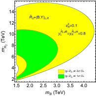
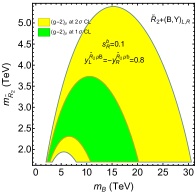
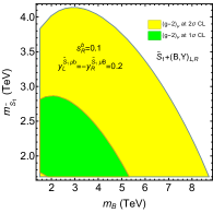
Figure 1: The $(g-2)_{\mu}$ allowed regions at $1\sigma$ (green) and $2\sigma$ (yellow) CLs with $s_{R}^{b}=0.1$. The parameters are chosen as $y_{L}^{\widetilde{R}_{2}\mu B}=y_{R}^{\widetilde{R}_{2}\mu b}=0.8$ in the $\widetilde{R}_{2}+(B,Y)$ model (left), $y_{L}^{\widetilde{R}_{2}\mu B}=-y_{R}^{\widetilde{R}_{2}\mu b}=0.8$ in the $\widetilde{R}_{2}+(B,Y)$ model (middle), and $y_{L}^{\widetilde{S}_{1}\mu b}=-y_{R}^{\widetilde{S}_{1}\mu B}=0.2$ in the $\widetilde{S}_{1}+(B,Y)$ model (right).

IV LQ and VLQ Phenomenology at hadron colliders

In Tab. 4, we list the main LQ and VLQ decay channels . The decay formulae of LQ and VLQ are given in App. A and B. For the scenario $m_{\mathrm{LQ}}>m_{B}$, there are new LQ decay channels. When searching for the LQ $\widetilde{R}_{2}^{2/3}$, we propose the $\mu j_{b}Z$ and $\mu j_{b}h$ signatures. When searching for the LQ $\widetilde{R}_{2}^{-1/3}$, we propose the $\mu j_{b}W$ signatures. When searching for the LQ $\widetilde{S}_{1}$, we propose the $\mu j_{b}Z$, $\mu j_{b}h$, $/\!\!\!\!{E_{T}}j_{b}W$ signatures. For the scenario $m_{\mathrm{LQ}}<m_{B}$, there are new VLQ decay channels. When searching for the VLQ $B$, we propose the $\mu^{+}\mu^{-}j_{b}$ signatures. When searching for the VLQ $Y$, we propose the $\mu~{}/\!\!\!\!{E_{T}}j_{b}$ signatures. It seems that such decay channels have not been searched by the experimental collaborations.

Model	Scenario	LQ decay	VLQ decay	new signatures
$\widetilde{R}_{2}+(B,Y)_{L,R}$	$m_{\mathrm{LQ}}>m_{B}$	$\widetilde{R}_{2}^{2/3}\rightarrow\mu^{+}b,\mu^{+}B$	$B\rightarrow bZ,bh$	$\widetilde{R}_{2}^{2/3}\rightarrow\mu j_{b}Z,\mu j_{b}h$
		$\widetilde{R}_{2}^{-1/3}\rightarrow\mu^{+}Y,\nu_{L}b$	$Y\rightarrow bW^{-}$	$\widetilde{R}_{2}^{-1/3}\rightarrow\mu j_{b}W$
	$m_{\mathrm{LQ}}<m_{B}$	$\widetilde{R}_{2}^{2/3}\rightarrow\mu^{+}b$	$B\rightarrow bZ,bh,\mu^{-}\widetilde{R}_{2}^{2/3}$	$B\rightarrow\mu^{+}\mu^{-}j_{b}$
		$\widetilde{R}_{2}^{-1/3}\rightarrow\nu_{L}b$	$Y\rightarrow bW^{-},\mu^{-}\widetilde{R}_{2}^{-1/3}$	$Y\rightarrow\mu~{}/\!\!\!\!{E_{T}}j_{b}$
$\widetilde{S}_{1}+(B,Y)_{L,R}$	$m_{\mathrm{LQ}}>m_{B}$	$\widetilde{S}_{1}\rightarrow\mu^{+}\bar{b},\mu^{+}\bar{B},\nu_{L}\bar{Y}$	$B\rightarrow bZ,bh$	$\widetilde{S}_{1}\rightarrow\mu j_{b}Z$, $\mu j_{b}h$, $/\!\!\!\!{E_{T}}j_{b}W$
			$Y\rightarrow bW^{-}$
	$m_{\mathrm{LQ}}<m_{B}$	$\widetilde{S}_{1}\rightarrow\mu^{+}\bar{b}$	$B\rightarrow bZ,bh,\mu^{+}(\widetilde{S}_{1})^{\ast}$	$B\rightarrow\mu^{+}\mu^{-}j_{b}$
			$Y\rightarrow bW^{-},\nu_{L}(\widetilde{S}_{1})^{\ast}$	$Y\rightarrow\mu~{}/\!\!\!\!{E_{T}}j_{b}$

Table 4: In the third column, we show the main LQ decay channels. In the fourth column, we show the main VLQ decay channels. In the fifth column, we show the new LQ or VLQ signatures.

To estimate the effects of new decay channels, we will compare the ratios of new partial decay widths to the tradition ones. Because of gauge symmetry, the different partial decay widths can be correlated. Then, we choose the following four ratios:

$$\frac{\Gamma(\widetilde{R}_{2}^{2/3}\rightarrow\mu^{+}B)}{\Gamma(\widetilde{R}_{2}^{2/3}\rightarrow\mu^{+}b)}\sim\frac{|y_{L}^{\widetilde{R}_{2}\mu B}|^{2}}{|y_{R}^{\widetilde{R}_{2}\mu b}|^{2}},\quad\frac{\Gamma(\widetilde{S}_{1}\rightarrow\mu^{+}\bar{B})}{\Gamma(\widetilde{S}_{1}\rightarrow\mu^{+}\bar{b})}\sim\frac{|y_{R}^{\widetilde{S}_{1}\mu B}|^{2}}{|y_{L}^{\widetilde{S}_{1}\mu b}|^{2}},$$

$$\frac{\Gamma(B\rightarrow\mu^{-}\widetilde{R}_{2}^{2/3})}{\Gamma(B\rightarrow bh)}\sim\frac{v^{2}|y_{L}^{\widetilde{R}_{2}\mu B}|^{2}}{m_{B}^{2}(s_{R}^{b})^{2}},\quad\frac{\Gamma(B\rightarrow\mu^{+}(\widetilde{S}_{1})^{\ast})}{\Gamma(B\rightarrow bh)}\sim\frac{v^{2}|y_{R}^{\widetilde{S}_{1}\mu B}|^{2}}{m_{B}^{2}(s_{R}^{b})^{2}}.$$ (34)

In Fig. 2, we show the contour plots of above four ratios under the consideration of $(g-2)_{\mu}$ constraints. In these plots, we have included the full contributions.

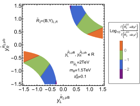
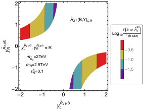
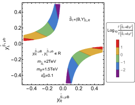
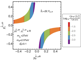
Figure 2: The contour plots of $\log_{10}\frac{\Gamma(\widetilde{R}_{2}^{2/3}\rightarrow\mu^{+}B)}{\Gamma(\widetilde{R}_{2}^{2/3}\rightarrow\mu^{+}b)}$ (upper left), $\log_{10}\frac{\Gamma(\widetilde{S}_{1}\rightarrow\mu^{+}\bar{B})}{\Gamma(\widetilde{S}_{1}\rightarrow\mu^{+}\bar{b})}$ (lower left), $\log_{10}\frac{\Gamma(B\rightarrow\mu^{-}\widetilde{R}_{2}^{2/3})}{\Gamma(B\rightarrow bh)}$ (upper right), and $\log_{10}\frac{\Gamma(B\rightarrow\mu^{+}(\widetilde{S}_{1})^{\ast})}{\Gamma(B\rightarrow bh)}$ (lower right), where the colored regions are allowed by the $(g-2)_{\mu}$ at $2\sigma$ CL. For the LQ decay, we choose $m_{B}=1.5\mathrm{TeV}$ and $m_{\mathrm{LQ}}=2\mathrm{TeV}$. For the VLQ decay, we choose $m_{B}=2.5\mathrm{TeV}$ and $m_{\mathrm{LQ}}=2\mathrm{TeV}$.

We find that the new LQ decay channels can become important for larger $|y_{L}^{\widetilde{R}_{2}\mu B}|$ in the $\widetilde{R}_{2}+(B,Y)_{L,R}$ model and $|y_{R}^{\widetilde{S}_{1}\mu B}|$ in the $\widetilde{S}_{1}+(B,Y)_{L,R}$ model. As to the VLQ decay, the importance of new decay channels depends on the $s_{R}^{b}$ sensitively. For $s_{R}^{b}=0.1$ and $m_{B}=2.5\mathrm{TeV}$, the new VLQ decay channels are less significant. For smaller $s_{R}^{b}$, the new VLQ decay channels can play the important role.

For the LQ and VLQ production at hadron colliders, there are pair and single production channels, which are very sensitive to the LQ and VLQ masses. We can adopt the FeynRules [54] to generate the model files and compute the cross sections with MadGraph5_-aMC@NLO [55]. For the 2 TeV scale LQ pair production [56, 57, 58], the cross section can be $\sim 0.01\mathrm{fb}$ at 13 TeV LHC. For the 1.5 TeV and 2.5 TeV scale VLQ pair production [59, 60, 61], the cross section can be $\sim 2\mathrm{fb}$ and $\sim 0.01\mathrm{fb}$ at 13 TeV LHC. For the single LQ and VLQ production channels, they depend on the electroweak couplings [62, 63, 42]. In the parameter space of large LQ Yukawa couplings, the single LQ production can be important, which may give some constraints at HL-LHC. To generate enough events, higher energy hadron colliders, for example 27 TeV and 100 TeV, can be necessary. Besides the collider direct search, there can be some indirect footprints, for example, $B$ physics related decay modes $\Upsilon\rightarrow\mu^{+}\mu^{-},\nu\bar{\nu}\gamma$. If we consider more complex flavour structure (say, turn on the $\mathrm{LQ}\mu s$ interaction), it can also affect the $B\rightarrow K\mu^{+}\mu^{-}$ channel. Here, we will not study these detailed phenomenology.

V Summary and conclusions

In this paper, we study the scalar LQ and VLQ extended models to explain the $(g-2)_{\mu}$ anomaly. Then, we find two new models $\widetilde{R}_{2}/\widetilde{S}_{1}+(B,Y)_{L,R}$, which can lead to the $B$ quark chiral enhancements because of the bottom and bottom partner mixing. During the numerical analysis, we consider two scenarios $m_{\mathrm{LQ}}>m_{B}$ and $m_{\mathrm{LQ}}<m_{B}$. After considering the experimental constraints, we choose relative light masses, which are adopted to be $(m_{B},m_{\mathrm{LQ}})=(1.5\mathrm{TeV},2\mathrm{TeV})$ for the first scenario and $(m_{B},m_{\mathrm{LQ}})=(2.5\mathrm{TeV},2\mathrm{TeV})$ for the second scenario. In the $\widetilde{R}_{2}+(B,Y)_{L,R}$ model, the $|\mathrm{Re}[y_{L}^{\widetilde{R}_{2}\mu B}(y_{R}^{\widetilde{R}_{2}\mu b})^{\ast}]|$ is bounded to be $\mathcal{O}(1)$, because $f_{LR}^{\widetilde{R}_{2}\mu b}(x)$ vanishes accidentally as $m_{B}=m_{\widetilde{R}_{2}}$. While, we can expect smaller $|\mathrm{Re}[y_{L}^{\widetilde{R}_{2}\mu B}(y_{R}^{\widetilde{R}_{2}\mu b})^{\ast}]|$ for largely splitted $m_{\widetilde{R}_{2}}$ and $m_{B}$. In the $\widetilde{S}_{1}+(B,Y)_{L,R}$ model, the $\mathrm{Re}[y_{R}^{\widetilde{S}_{1}\mu B}(y_{L}^{\widetilde{S}_{1}\mu b})^{\ast}]$ is bounded to be the range $(-0.06,-0.02)$ at $2\sigma$ CL if $s_{R}^{b}=0.1$.

Under the constraints from $(g-2)_{\mu}$, we propose new LQ and VLQ search channels. In the scenario $m_{\mathrm{LQ}}>m_{B}$, there are new LQ decay channels: $\widetilde{R}_{2}^{2/3}\rightarrow\mu^{+}B$, $\widetilde{R}_{2}^{-1/3}\rightarrow\mu^{+}Y$, and $\widetilde{S}_{1}\rightarrow\mu^{+}\bar{B},\nu_{L}\bar{Y}$. For larger $y_{L}^{\widetilde{R}_{2}\mu B}$ and $y_{R}^{\widetilde{S}_{1}\mu B}$, it is important to take into account these decay channels. In the scenario $m_{\mathrm{LQ}}<m_{B}$, there are new VLQ decay channels: $B\rightarrow\mu^{-}\widetilde{R}_{2}^{2/3},\mu^{+}(\widetilde{S}_{1})^{\ast}$ and $Y\rightarrow\mu^{-}\widetilde{R}_{2}^{-1/3},\nu_{L}(\widetilde{S}_{1})^{\ast}$. For $s_{R}^{b}=0.1$, these channels are negligible compared to the traditional $B\rightarrow bZ,bh$ and $Y\rightarrow bW^{-}$ channels. For smaller $s_{R}^{b}$, these new VLQ decay channels can also become important.

Note added: In paper [64], the authors study the model with $\widetilde{R}_{2}$, $S_{3}$, and $(B,Y)_{L,R}$. In their work, they do not consider the bottom and $B$ quark mixing, and the chiral enhancements are produced through the $\widetilde{R}_{2}$ and $S_{3}$ mixing. In paper [65], the authors explain the $(g-2)_{\mu}$ and $B$ physics anomalies in the $S_{1}+(B,Y)_{L,R}$ model.

Appendix A LQ decay width formulae

When the $\widetilde{R}_{2}$ masses are degenerate, there are no gauge boson decay channels such as $\widetilde{R}_{2}^{2/3}\rightarrow\widetilde{R}_{2}^{-1/3}W^{+}$. For the $\widetilde{R}_{2}^{2/3}$ to $\mu^{+}b$ and $\mu^{+}B$ decay channels, the widths are calculated as

$$\Gamma(\widetilde{R}_{2}^{2/3}\rightarrow\mu^{+}b)=\frac{m_{\widetilde{R}_{2}}}{16\pi}\sqrt{(1-\frac{m_{\mu}^{2}+m_{b}^{2}}{m_{\widetilde{R}_{2}}^{2}})^{2}-\frac{4m_{\mu}^{2}m_{b}^{2}}{m_{\widetilde{R}_{2}}^{4}}}~{}\cdot$$

$$\Big{\{}(1-\frac{m_{\mu}^{2}+m_{b}^{2}}{m_{\widetilde{R}_{2}}^{2}})[|y_{L}^{\widetilde{R}_{2}\mu B}|^{2}(s_{L}^{b})^{2}+|y_{R}^{\widetilde{R}_{2}\mu b}|^{2}(c_{R}^{b})^{2}]+\frac{4m_{\mu}m_{b}}{m_{\widetilde{R}_{2}}^{2}}s_{L}^{b}c_{R}^{b}\mathrm{Re}[y_{L}^{\widetilde{R}_{2}\mu B}(y_{R}^{\widetilde{R}_{2}\mu b})^{\ast}]\Big{\}},$$

$$\Gamma(\widetilde{R}_{2}^{2/3}\rightarrow\mu^{+}B)=\frac{m_{\widetilde{R}_{2}}}{16\pi}\sqrt{(1-\frac{m_{\mu}^{2}+m_{B}^{2}}{m_{\widetilde{R}_{2}}^{2}})^{2}-\frac{4m_{\mu}^{2}m_{B}^{2}}{m_{\widetilde{R}_{2}}^{4}}}~{}\cdot$$

$$\Big{\{}(1-\frac{m_{\mu}^{2}+m_{B}^{2}}{m_{\widetilde{R}_{2}}^{2}})[|y_{L}^{\widetilde{R}_{2}\mu B}|^{2}(c_{L}^{b})^{2}+|y_{R}^{\widetilde{R}_{2}\mu b}|^{2}(s_{R}^{b})^{2}]-\frac{4m_{\mu}m_{B}}{m_{\widetilde{R}_{2}}^{2}}c_{L}^{b}s_{R}^{b}\mathrm{Re}[y_{L}^{\widetilde{R}_{2}\mu B}(y_{R}^{\widetilde{R}_{2}\mu b})^{\ast}]\Big{\}}.$$ (35)

For the $\widetilde{R}_{2}^{-1/3}$ to $\mu^{+}Y,\nu_{L}b,\nu_{L}B$ decay channels, the widths are calculated as

$$\Gamma(\widetilde{R}_{2}^{-1/3}\rightarrow\mu^{+}Y)=\frac{m_{\widetilde{R}_{2}}}{16\pi}\sqrt{(1-\frac{m_{\mu}^{2}+m_{Y}^{2}}{m_{\widetilde{R}_{2}}^{2}})^{2}-\frac{4m_{\mu}^{2}m_{Y}^{2}}{m_{\widetilde{R}_{2}}^{4}}}(1-\frac{m_{\mu}^{2}+m_{Y}^{2}}{m_{\widetilde{R}_{2}}^{2}})|y_{L}^{\widetilde{R}_{2}\mu B}|^{2},$$

$$\Gamma(\widetilde{R}_{2}^{-1/3}\rightarrow\nu_{L}b)=\frac{m_{\widetilde{R}_{2}}}{16\pi}(1-\frac{m_{b}^{2}}{m_{\widetilde{R}_{2}}^{2}})^{2}|y_{R}^{\widetilde{R}_{2}\mu b}|^{2}(c_{R}^{b})^{2},$$

$$\Gamma(\widetilde{R}_{2}^{-1/3}\rightarrow\nu_{L}B)=\frac{m_{\widetilde{R}_{2}}}{16\pi}(1-\frac{m_{B}^{2}}{m_{\widetilde{R}_{2}}^{2}})^{2}|y_{R}^{\widetilde{R}_{2}\mu b}|^{2}(s_{R}^{b})^{2}.$$ (36)

Considering $m_{\mu},m_{b}\ll m_{B}$ and $\theta_{L,R}^{b}\ll 1$, we have the following approximations:

$$\Gamma(\widetilde{R}_{2}^{2/3}\rightarrow\mu^{+}B)\approx\Gamma(\widetilde{R}_{2}^{-1/3}\rightarrow\mu^{+}Y)\approx\frac{m_{\widetilde{R}_{2}}}{16\pi}(1-\frac{m_{B}^{2}}{m_{\widetilde{R}_{2}}^{2}})^{2}|y_{L}^{\widetilde{R}_{2}\mu B}|^{2},$$

$$\Gamma(\widetilde{R}_{2}^{2/3}\rightarrow\mu^{+}b)\approx\Gamma(\widetilde{R}_{2}^{-1/3}\rightarrow\nu_{L}b)\approx\frac{m_{\widetilde{R}_{2}}}{16\pi}|y_{R}^{\widetilde{R}_{2}\mu b}|^{2}.$$ (37)

For the $\widetilde{S}_{1}$ to $\mu^{+}\bar{b},\mu^{+}\bar{B},\nu_{L}\bar{Y}$ decay channels, the widths are calculated as

$$\Gamma(\widetilde{S}_{1}\rightarrow\mu^{+}\bar{b})=\frac{m_{\widetilde{S}_{1}}}{16\pi}\sqrt{(1-\frac{m_{\mu}^{2}+m_{b}^{2}}{m_{\widetilde{S}_{1}}^{2}})^{2}-\frac{4m_{\mu}^{2}m_{b}^{2}}{m_{\widetilde{S}_{1}}^{4}}}~{}\cdot$$

$$\Big{\{}(1-\frac{m_{\mu}^{2}+m_{b}^{2}}{m_{\widetilde{S}_{1}}^{2}})[|y_{R}^{\widetilde{S}_{1}\mu B}|^{2}(s_{L}^{b})^{2}+|y_{L}^{\widetilde{S}_{1}\mu b}|^{2}(c_{R}^{b})^{2}]+\frac{4m_{\mu}m_{b}}{m_{\widetilde{S}_{1}}^{2}}s_{L}^{b}c_{R}^{b}\mathrm{Re}[y_{R}^{\widetilde{S}_{1}\mu B}(y_{L}^{\widetilde{S}_{1}\mu b})^{\ast}]\Big{\}},$$

$$\Gamma(\widetilde{S}_{1}\rightarrow\mu^{+}\bar{B})=\frac{m_{\widetilde{S}_{1}}}{16\pi}\sqrt{(1-\frac{m_{\mu}^{2}+m_{B}^{2}}{m_{\widetilde{S}_{1}}^{2}})^{2}-\frac{4m_{\mu}^{2}m_{B}^{2}}{m_{\widetilde{S}_{1}}^{4}}}~{}\cdot$$

$$\Big{\{}(1-\frac{m_{\mu}^{2}+m_{B}^{2}}{m_{\widetilde{S}_{1}}^{2}})[|y_{R}^{\widetilde{S}_{1}\mu B}|^{2}(c_{L}^{b})^{2}+|y_{L}^{\widetilde{S}_{1}\mu b}|^{2}(s_{R}^{b})^{2}]-\frac{4m_{\mu}m_{B}}{m_{\widetilde{S}_{1}}^{2}}c_{L}^{b}s_{R}^{b}\mathrm{Re}[y_{R}^{\widetilde{S}_{1}\mu B}(y_{L}^{\widetilde{S}_{1}\mu b})^{\ast}]\Big{\}},$$

$$\Gamma(\widetilde{S}_{1}\rightarrow\nu_{L}\bar{Y})=\frac{m_{\widetilde{S}_{1}}}{16\pi}(1-\frac{m_{Y}^{2}}{m_{\widetilde{S}_{1}}^{2}})^{2}|y_{R}^{\widetilde{S}_{1}\mu B}|^{2}.$$ (38)

Considering $m_{\mu},m_{b}\ll m_{B}$ and $\theta_{L,R}^{b}\ll 1$, we have the following approximations:

$$\Gamma(\widetilde{S}_{1}\rightarrow\mu^{+}\bar{B})\approx\Gamma(\widetilde{S}_{1}\rightarrow\nu_{L}\bar{Y})\approx\frac{m_{\widetilde{S}_{1}}}{16\pi}(1-\frac{m_{B}^{2}}{m_{\widetilde{S}_{1}}^{2}})^{2}|y_{R}^{\widetilde{S}_{1}\mu B}|^{2},$$

$$\Gamma(\widetilde{S}_{1}\rightarrow\mu^{+}\bar{b})\approx\frac{m_{\widetilde{S}_{1}}}{16\pi}|y_{L}^{\widetilde{S}_{1}\mu b}|^{2}.$$ (39)

Appendix B VLQ decay width formulae

If $m_{B}\sim\mathrm{TeV}$ and $\theta_{R}^{b}\ll 0.1$, we have $m_{B}-m_{Y}\approx m_{B}(s_{R}^{b})^{2}/2\lesssim 5\mathrm{GeV}$, which leads to the kinematic prohibition of some decay channels. For the $Y\rightarrow bW^{-}$ decay channel, the width is calculated as

$$\Gamma(Y\rightarrow bW^{-})=\frac{g^{2}}{64\pi m_{Y}}\sqrt{(1-\frac{m_{b}^{2}+m_{W}^{2}}{m_{Y}^{2}})^{2}-\frac{4m_{b}^{2}m_{W}^{2}}{m_{Y}^{4}}}\cdot$$

$$\Big{\{}[(s_{L}^{b})^{2}+(s_{R}^{b})^{2}]\frac{(m_{Y}^{2}-m_{b}^{2})^{2}+m_{W}^{2}(m_{Y}^{2}+m_{b}^{2})-2m_{W}^{4}}{m_{W}^{2}}-12m_{Y}m_{b}s_{L}^{b}s_{R}^{b}\Big{\}}.$$ (40)

For the $B\rightarrow bZ,bh,tW^{-}$ decay channels, the widths are calculated as

$$\Gamma(B\rightarrow bh)=\frac{m_{B}}{32\pi}\sqrt{(1-\frac{m_{b}^{2}+m_{h}^{2}}{m_{B}^{2}})^{2}-\frac{4m_{b}^{2}m_{h}^{2}}{m_{B}^{4}}}\Big{[}(1+\frac{m_{b}^{2}-m_{h}^{2}}{m_{B}^{2}})\frac{m_{b}^{2}+m_{B}^{2}}{v^{2}}+4\frac{m_{b}^{2}}{v^{2}}\big{)}\Big{]}(s_{R}^{b})^{2}(c_{R}^{b})^{2},$$

$$\Gamma(B\rightarrow bZ)=\frac{g^{2}}{32\pi c_{W}^{2}m_{B}}\sqrt{(1-\frac{m_{b}^{2}+m_{Z}^{2}}{m_{B}^{2}})^{2}-\frac{4m_{b}^{2}m_{Z}^{2}}{m_{B}^{4}}}\cdot$$

$$\Big{\{}[(s_{L}^{b}c_{L}^{b})^{2}+\frac{(s_{R}^{b}c_{R}^{b})^{2}}{4}]\frac{(m_{B}^{2}-m_{b}^{2})^{2}+m_{Z}^{2}(m_{B}^{2}+m_{b}^{2})-2m_{Z}^{4}}{m_{Z}^{2}}-6m_{B}m_{b}s_{L}^{b}s_{R}^{b}c_{L}^{b}c_{R}^{b}\Big{\}},$$

$$\Gamma(B\rightarrow tW^{-})=\frac{g^{2}(s_{L}^{b})^{2}}{64\pi}\sqrt{(1-\frac{m_{t}^{2}+m_{W}^{2}}{m_{B}^{2}})^{2}-\frac{4m_{t}^{2}m_{W}^{2}}{m_{B}^{4}}}\frac{(m_{B}^{2}-m_{t}^{2})^{2}+m_{W}^{2}(m_{B}^{2}+m_{t}^{2})-2m_{W}^{4}}{m_{W}^{2}m_{B}}.$$ (41)

Considering $m_{b},m_{t},m_{Z},m_{W}\ll m_{B}$ and $\theta_{L,R}^{b}\ll 1$, we have the following approximations:

$$\Gamma(B\rightarrow bZ)\approx\Gamma(B\rightarrow bh)\approx\frac{1}{2}\Gamma(Y\rightarrow bW^{-})\approx\frac{m_{B}^{3}}{32\pi v^{2}}(s_{R}^{b})^{2},$$

$$\Gamma(B\rightarrow tW^{-})\approx\frac{m_{b}^{2}m_{B}}{16\pi v^{2}}(s_{R}^{b})^{2}.$$ (42)

In the $\widetilde{R}_{2}+(B,Y)_{L,R}$ model, the VLQ can also decay into $\widetilde{R}_{2}$ final state. For the $Y\rightarrow\mu^{-}\widetilde{R}_{2}^{-1/3}$ decay channel, the width is calculated as

$$\Gamma(Y\rightarrow\mu^{-}\widetilde{R}_{2}^{-1/3})=\frac{m_{Y}}{32\pi}\sqrt{(1-\frac{m_{\mu}^{2}+m_{\widetilde{R}_{2}}^{2}}{m_{Y}^{2}})^{2}-\frac{4m_{\mu}^{2}m_{\widetilde{R}_{2}}^{2}}{m_{Y}^{4}}}(1+\frac{m_{\mu}^{2}-m_{\widetilde{R}_{2}}^{2}}{m_{Y}^{2}})|y_{L}^{\widetilde{R}_{2}\mu B}|^{2}.$$ (43)

For the $B\rightarrow\mu^{-}\widetilde{R}_{2}^{2/3},\nu_{L}\widetilde{R}_{2}^{-1/3}$ decay channels, the widths are calculated as

$$\Gamma(B\rightarrow\mu^{-}\widetilde{R}_{2}^{2/3})=\frac{m_{B}}{32\pi}\sqrt{(1-\frac{m_{\mu}^{2}+m_{\widetilde{R}_{2}}^{2}}{m_{B}^{2}})^{2}-\frac{4m_{\mu}^{2}m_{\widetilde{R}_{2}}^{2}}{m_{B}^{4}}}~{}\cdot$$

$$\Big{\{}(1+\frac{m_{\mu}^{2}-m_{\widetilde{R}_{2}}^{2}}{m_{B}^{2}})[|y_{L}^{\widetilde{R}_{2}\mu B}|^{2}(c_{L}^{b})^{2}+|y_{R}^{\widetilde{R}_{2}\mu b}|^{2}(s_{R}^{b})^{2}]+\frac{4m_{\mu}m_{\widetilde{R}_{2}}}{m_{B}^{2}}c_{L}^{b}s_{R}^{b}\mathrm{Re}[y_{L}^{\widetilde{R}_{2}\mu B}(y_{R}^{\widetilde{R}_{2}\mu b})^{\ast}]\Big{\}},$$

$$\Gamma(B\rightarrow\nu_{L}\widetilde{R}_{2}^{-1/3})=\frac{m_{B}}{32\pi}(1-\frac{m_{\widetilde{R}_{2}}^{2}}{m_{B}^{2}})^{2}|y_{R}^{\widetilde{R}_{2}\mu b}|^{2}(s_{R}^{b})^{2}.$$ (44)

Considering $m_{\mu}\ll m_{B}$ and $\theta_{L,R}^{b}\ll 1$, we have the following approximations:

$$\Gamma(B\rightarrow\mu^{-}\widetilde{R}_{2}^{2/3})\approx\Gamma(Y\rightarrow\mu^{-}\widetilde{R}_{2}^{-1/3})\approx\frac{m_{B}}{32\pi}(1-\frac{m_{\widetilde{R}_{2}}^{2}}{m_{B}^{2}})^{2}|y_{L}^{\widetilde{R}_{2}\mu B}|^{2}.$$ (45)

In the $\widetilde{S}_{1}+(B,Y)_{L,R}$ model, the VLQ can also decay into $\widetilde{S}_{1}$ final state. For the $Y\rightarrow\nu_{L}(\widetilde{S}_{1})^{\ast}$ decay channel, the width is calculated as

$$\Gamma(Y\rightarrow\nu_{L}(\widetilde{S}_{1})^{\ast})=\frac{m_{Y}}{32\pi}(1-\frac{m_{\widetilde{S}_{1}}^{2}}{m_{Y}^{2}})^{2}|y_{R}^{\widetilde{S}_{1}\mu B}|^{2}.$$ (46)

For the $B\rightarrow\mu^{+}(\widetilde{S}_{1})^{\ast}$ decay channel, the width is calculated as

$$\Gamma(B\rightarrow\mu^{+}(\widetilde{S}_{1})^{\ast})=\frac{m_{B}}{32\pi}\sqrt{(1-\frac{m_{\mu}^{2}+m_{\widetilde{S}_{1}}^{2}}{m_{B}^{2}})^{2}-\frac{4m_{\mu}^{2}m_{\widetilde{S}_{1}}^{2}}{m_{B}^{4}}}~{}\cdot$$

$$\Big{\{}(1+\frac{m_{\mu}^{2}-m_{\widetilde{S}_{1}}^{2}}{m_{B}^{2}})[|y_{R}^{\widetilde{S}_{1}\mu B}|^{2}(c_{L}^{b})^{2}+|y_{L}^{\widetilde{S}_{1}\mu b}|^{2}(s_{R}^{b})^{2}]+\frac{4m_{\mu}}{m_{B}}c_{L}^{b}s_{R}^{b}\mathrm{Re}[y_{R}^{\widetilde{S}_{1}\mu B}(y_{L}^{\widetilde{S}_{1}\mu b})^{\ast}]\Big{\}}.$$ (47)

Considering $m_{\mu}\ll m_{B}$ and $\theta_{L,R}^{b}\ll 1$, we have the following approximations:

$$\Gamma(B\rightarrow\mu^{+}(\widetilde{S}_{1})^{\ast})\approx\Gamma(Y\rightarrow\nu_{L}(\widetilde{S}_{1})^{\ast})\approx\frac{m_{B}}{32\pi}(1-\frac{m_{\widetilde{S}_{1}}^{2}}{m_{B}^{2}})^{2}|y_{R}^{\widetilde{S}_{1}\mu B}|^{2}.$$ (48)

References

- Bennett et al. [2006] G. W. Bennett et al. (Muon g-2), Final Report of the Muon E821 Anomalous Magnetic Moment Measurement at BNL, Phys. Rev. D 73, 072003 (2006), arXiv:hep-ex/0602035 .
- Abi et al. [2021] B. Abi et al. (Muon g-2), Measurement of the Positive Muon Anomalous Magnetic Moment to 0.46 ppm, Phys. Rev. Lett. 126, 141801 (2021), arXiv:2104.03281 [hep-ex] .
- Aoyama et al. [2012] T. Aoyama, M. Hayakawa, T. Kinoshita, and M. Nio, Complete Tenth-Order QED Contribution to the Muon g-2, Phys. Rev. Lett. 109, 111808 (2012), arXiv:1205.5370 [hep-ph] .
- Aoyama et al. [2019] T. Aoyama, T. Kinoshita, and M. Nio, Theory of the Anomalous Magnetic Moment of the Electron, Atoms 7, 28 (2019).
- Czarnecki et al. [2003] A. Czarnecki, W. J. Marciano, and A. Vainshtein, Refinements in electroweak contributions to the muon anomalous magnetic moment, Phys. Rev. D 67, 073006 (2003), [Erratum: Phys.Rev.D 73, 119901 (2006)], arXiv:hep-ph/0212229 .
- Gnendiger et al. [2013] C. Gnendiger, D. Stöckinger, and H. Stöckinger-Kim, The electroweak contributions to after the Higgs boson mass measurement, Phys. Rev. D 88, 053005 (2013), arXiv:1306.5546 [hep-ph] .
- Davier et al. [2017] M. Davier, A. Hoecker, B. Malaescu, and Z. Zhang, Reevaluation of the hadronic vacuum polarisation contributions to the Standard Model predictions of the muon and using newest hadronic cross-section data, Eur. Phys. J. C 77, 827 (2017), arXiv:1706.09436 [hep-ph] .
- Keshavarzi et al. [2018] A. Keshavarzi, D. Nomura, and T. Teubner, Muon and : a new data-based analysis, Phys. Rev. D 97, 114025 (2018), arXiv:1802.02995 [hep-ph] .
- Colangelo et al. [2019] G. Colangelo, M. Hoferichter, and P. Stoffer, Two-pion contribution to hadronic vacuum polarization, JHEP 02, 006, arXiv:1810.00007 [hep-ph] .
- Hoferichter et al. [2019] M. Hoferichter, B.-L. Hoid, and B. Kubis, Three-pion contribution to hadronic vacuum polarization, JHEP 08, 137, arXiv:1907.01556 [hep-ph] .
- Davier et al. [2020] M. Davier, A. Hoecker, B. Malaescu, and Z. Zhang, A new evaluation of the hadronic vacuum polarisation contributions to the muon anomalous magnetic moment and to , Eur. Phys. J. C 80, 241 (2020), [Erratum: Eur.Phys.J.C 80, 410 (2020)], arXiv:1908.00921 [hep-ph] .
- Keshavarzi et al. [2020] A. Keshavarzi, D. Nomura, and T. Teubner, of charged leptons, , and the hyperfine splitting of muonium, Phys. Rev. D 101, 014029 (2020), arXiv:1911.00367 [hep-ph] .
- Kurz et al. [2014] A. Kurz, T. Liu, P. Marquard, and M. Steinhauser, Hadronic contribution to the muon anomalous magnetic moment to next-to-next-to-leading order, Phys. Lett. B 734, 144 (2014), arXiv:1403.6400 [hep-ph] .
- Melnikov and Vainshtein [2004] K. Melnikov and A. Vainshtein, Hadronic light-by-light scattering contribution to the muon anomalous magnetic moment revisited, Phys. Rev. D 70, 113006 (2004), arXiv:hep-ph/0312226 .
- Masjuan and Sanchez-Puertas [2017] P. Masjuan and P. Sanchez-Puertas, Pseudoscalar-pole contribution to the : a rational approach, Phys. Rev. D 95, 054026 (2017), arXiv:1701.05829 [hep-ph] .
- Colangelo et al. [2017] G. Colangelo, M. Hoferichter, M. Procura, and P. Stoffer, Dispersion relation for hadronic light-by-light scattering: two-pion contributions, JHEP 04, 161, arXiv:1702.07347 [hep-ph] .
- Hoferichter et al. [2018] M. Hoferichter, B.-L. Hoid, B. Kubis, S. Leupold, and S. P. Schneider, Dispersion relation for hadronic light-by-light scattering: pion pole, JHEP 10, 141, arXiv:1808.04823 [hep-ph] .
- Gérardin et al. [2019] A. Gérardin, H. B. Meyer, and A. Nyffeler, Lattice calculation of the pion transition form factor with Wilson quarks, Phys. Rev. D 100, 034520 (2019), arXiv:1903.09471 [hep-lat] .
- Bijnens et al. [2019] J. Bijnens, N. Hermansson-Truedsson, and A. Rodríguez-Sánchez, Short-distance constraints for the HLbL contribution to the muon anomalous magnetic moment, Phys. Lett. B 798, 134994 (2019), arXiv:1908.03331 [hep-ph] .
- Colangelo et al. [2020] G. Colangelo, F. Hagelstein, M. Hoferichter, L. Laub, and P. Stoffer, Longitudinal short-distance constraints for the hadronic light-by-light contribution to with large- Regge models, JHEP 03, 101, arXiv:1910.13432 [hep-ph] .
- Blum et al. [2020] T. Blum, N. Christ, M. Hayakawa, T. Izubuchi, L. Jin, C. Jung, and C. Lehner, Hadronic Light-by-Light Scattering Contribution to the Muon Anomalous Magnetic Moment from Lattice QCD, Phys. Rev. Lett. 124, 132002 (2020), arXiv:1911.08123 [hep-lat] .
- Colangelo et al. [2014] G. Colangelo, M. Hoferichter, A. Nyffeler, M. Passera, and P. Stoffer, Remarks on higher-order hadronic corrections to the muon g2, Phys. Lett. B 735, 90 (2014), arXiv:1403.7512 [hep-ph] .
- Aoyama et al. [2020] T. Aoyama et al., The anomalous magnetic moment of the muon in the Standard Model, Phys. Rept. 887, 1 (2020), arXiv:2006.04822 [hep-ph] .
- Czarnecki and Marciano [2001] A. Czarnecki and W. J. Marciano, The Muon anomalous magnetic moment: A Harbinger for ’new physics’, Phys. Rev. D 64, 013014 (2001), arXiv:hep-ph/0102122 .
- Jegerlehner and Nyffeler [2009] F. Jegerlehner and A. Nyffeler, The Muon g-2, Phys. Rept. 477, 1 (2009), arXiv:0902.3360 [hep-ph] .
- Freitas et al. [2014] A. Freitas, J. Lykken, S. Kell, and S. Westhoff, Testing the Muon g-2 Anomaly at the LHC, JHEP 05, 145, [Erratum: JHEP 09, 155 (2014)], arXiv:1402.7065 [hep-ph] .
- Queiroz and Shepherd [2014] F. S. Queiroz and W. Shepherd, New Physics Contributions to the Muon Anomalous Magnetic Moment: A Numerical Code, Phys. Rev. D 89, 095024 (2014), arXiv:1403.2309 [hep-ph] .
- Lindner et al. [2018] M. Lindner, M. Platscher, and F. S. Queiroz, A Call for New Physics : The Muon Anomalous Magnetic Moment and Lepton Flavor Violation, Phys. Rept. 731, 1 (2018), arXiv:1610.06587 [hep-ph] .
- Athron et al. [2021] P. Athron, C. Balázs, D. H. Jacob, W. Kotlarski, D. Stöckinger, and H. Stöckinger-Kim, New physics explanations of in light of the FNAL muon measurement, JHEP 09, 080, arXiv:2104.03691 [hep-ph] .
- Kannike et al. [2012] K. Kannike, M. Raidal, D. M. Straub, and A. Strumia, Anthropic solution to the magnetic muon anomaly: the charged see-saw, JHEP 02, 106, [Erratum: JHEP 10, 136 (2012)], arXiv:1111.2551 [hep-ph] .
- Frank and Saha [2020] M. Frank and I. Saha, Muon anomalous magnetic moment in two-Higgs-doublet models with vectorlike leptons, Phys. Rev. D 102, 115034 (2020), arXiv:2008.11909 [hep-ph] .
- Dermisek et al. [2021] R. Dermisek, K. Hermanek, and N. McGinnis, Muon g-2 in two-Higgs-doublet models with vectorlike leptons, Phys. Rev. D 104, 055033 (2021), arXiv:2103.05645 [hep-ph] .
- Crivellin and Hoferichter [2021] A. Crivellin and M. Hoferichter, Consequences of chirally enhanced explanations of for h → and Z → , JHEP 07, 135, [Erratum: JHEP 10, 030 (2022)], arXiv:2104.03202 [hep-ph] .
- Cheung [2001] K.-m. Cheung, Muon anomalous magnetic moment and leptoquark solutions, Phys. Rev. D 64, 033001 (2001), arXiv:hep-ph/0102238 .
- Doršner et al. [2016] I. Doršner, S. Fajfer, A. Greljo, J. F. Kamenik, and N. Košnik, Physics of leptoquarks in precision experiments and at particle colliders, Phys. Rept. 641, 1 (2016), arXiv:1603.04993 [hep-ph] .
- Coluccio Leskow et al. [2017] E. Coluccio Leskow, G. D’Ambrosio, A. Crivellin, and D. Müller, , lepton flavor violation, and decays with leptoquarks: Correlations and future prospects, Phys. Rev. D 95, 055018 (2017), arXiv:1612.06858 [hep-ph] .
- Doršner et al. [2020a] I. Doršner, S. Fajfer, and O. Sumensari, Muon and scalar leptoquark mixing, JHEP 06, 089, arXiv:1910.03877 [hep-ph] .
- Crivellin et al. [2021] A. Crivellin, D. Mueller, and F. Saturnino, Correlating h→+- to the Anomalous Magnetic Moment of the Muon via Leptoquarks, Phys. Rev. Lett. 127, 021801 (2021), arXiv:2008.02643 [hep-ph] .
- Doršner et al. [2020b] I. Doršner, S. Fajfer, and S. Saad, selecting scalar leptoquark solutions for the puzzles, Phys. Rev. D 102, 075007 (2020b), arXiv:2006.11624 [hep-ph] .
- Zhang [2021] D. Zhang, Radiative neutrino masses, lepton flavor mixing and muon g 2 in a leptoquark model, JHEP 07, 069, arXiv:2105.08670 [hep-ph] .
- He [2022] S.-P. He, Leptoquark and vectorlike quark extended models as the explanation of the muon anomaly, Phys. Rev. D 105, 035017 (2022), [Erratum: Phys.Rev.D 106, 039901 (2022)], arXiv:2112.13490 [hep-ph] .
- Aguilar-Saavedra et al. [2013] J. A. Aguilar-Saavedra, R. Benbrik, S. Heinemeyer, and M. Pérez-Victoria, Handbook of vectorlike quarks: Mixing and single production, Phys. Rev. D 88, 094010 (2013), arXiv:1306.0572 [hep-ph] .
- Workman [2022] R. L. Workman (Particle Data Group), Review of Particle Physics, PTEP 2022, 083C01 (2022).
- Sirunyan et al. [2020] A. M. Sirunyan et al. (CMS), A search for bottom-type, vector-like quark pair production in a fully hadronic final state in proton-proton collisions at 13 TeV, Phys. Rev. D 102, 112004 (2020), arXiv:2008.09835 [hep-ex] .
- Sirunyan et al. [2017] A. M. Sirunyan et al. (CMS), Search for single production of vector-like quarks decaying into a b quark and a W boson in proton-proton collisions at 13 TeV, Phys. Lett. B 772, 634 (2017), arXiv:1701.08328 [hep-ex] .
- Aaboud et al. [2018] M. Aaboud et al. (ATLAS), Combination of the searches for pair-produced vector-like partners of the third-generation quarks at 13 TeV with the ATLAS detector, Phys. Rev. Lett. 121, 211801 (2018), arXiv:1808.02343 [hep-ex] .
- Aaboud et al. [2019] M. Aaboud et al. (ATLAS), Search for single production of vector-like quarks decaying into in collisions at TeV with the ATLAS detector, JHEP 05, 164, arXiv:1812.07343 [hep-ex] .
- Chen et al. [2017] C.-Y. Chen, S. Dawson, and E. Furlan, Vectorlike fermions and Higgs effective field theory revisited, Phys. Rev. D 96, 015006 (2017), arXiv:1703.06134 [hep-ph] .
- Cao et al. [2022] J. Cao, L. Meng, L. Shang, S. Wang, and B. Yang, Interpreting the W-mass anomaly in vectorlike quark models, Phys. Rev. D 106, 055042 (2022), arXiv:2204.09477 [hep-ph] .
- Schael et al. [2006] S. Schael et al. (ALEPH, DELPHI, L3, OPAL, SLD, LEP Electroweak Working Group, SLD Electroweak Group, SLD Heavy Flavour Group), Precision electroweak measurements on the resonance, Phys. Rept. 427, 257 (2006), arXiv:hep-ex/0509008 .
- Baak et al. [2014] M. Baak, J. Cúth, J. Haller, A. Hoecker, R. Kogler, K. Mönig, M. Schott, and J. Stelzer (Gfitter Group), The global electroweak fit at NNLO and prospects for the LHC and ILC, Eur. Phys. J. C 74, 3046 (2014), arXiv:1407.3792 [hep-ph] .
- Sirunyan et al. [2019] A. M. Sirunyan et al. (CMS), Search for pair production of second-generation leptoquarks at 13 TeV, Phys. Rev. D 99, 032014 (2019), arXiv:1808.05082 [hep-ex] .
- Aad et al. [2020] G. Aad et al. (ATLAS), Search for pairs of scalar leptoquarks decaying into quarks and electrons or muons in = 13 TeV collisions with the ATLAS detector, JHEP 10, 112, arXiv:2006.05872 [hep-ex] .
- Alloul et al. [2014] A. Alloul, N. D. Christensen, C. Degrande, C. Duhr, and B. Fuks, FeynRules 2.0 - A complete toolbox for tree-level phenomenology, Comput. Phys. Commun. 185, 2250 (2014), arXiv:1310.1921 [hep-ph] .
- Alwall et al. [2014] J. Alwall, R. Frederix, S. Frixione, V. Hirschi, F. Maltoni, O. Mattelaer, H. S. Shao, T. Stelzer, P. Torrielli, and M. Zaro, The automated computation of tree-level and next-to-leading order differential cross sections, and their matching to parton shower simulations, JHEP 07, 079, arXiv:1405.0301 [hep-ph] .
- Blumlein et al. [1997] J. Blumlein, E. Boos, and A. Kryukov, Leptoquark pair production in hadronic interactions, Z. Phys. C 76, 137 (1997), arXiv:hep-ph/9610408 .
- Diaz et al. [2017] B. Diaz, M. Schmaltz, and Y.-M. Zhong, The leptoquark Hunter’s guide: Pair production, JHEP 10, 097, arXiv:1706.05033 [hep-ph] .
- Doršner and Greljo [2018] I. Doršner and A. Greljo, Leptoquark toolbox for precision collider studies, JHEP 05, 126, arXiv:1801.07641 [hep-ph] .
- Aguilar-Saavedra [2009] J. A. Aguilar-Saavedra, Identifying top partners at LHC, JHEP 11, 030, arXiv:0907.3155 [hep-ph] .
- Matsedonskyi et al. [2014] O. Matsedonskyi, G. Panico, and A. Wulzer, On the Interpretation of Top Partners Searches, JHEP 12, 097, arXiv:1409.0100 [hep-ph] .
- Fuks and Shao [2017] B. Fuks and H.-S. Shao, QCD next-to-leading-order predictions matched to parton showers for vector-like quark models, Eur. Phys. J. C 77, 135 (2017), arXiv:1610.04622 [hep-ph] .
- Buonocore et al. [2020] L. Buonocore, U. Haisch, P. Nason, F. Tramontano, and G. Zanderighi, Lepton-Quark Collisions at the Large Hadron Collider, Phys. Rev. Lett. 125, 231804 (2020), arXiv:2005.06475 [hep-ph] .
- Buonocore et al. [2022] L. Buonocore, A. Greljo, P. Krack, P. Nason, N. Selimovic, F. Tramontano, and G. Zanderighi, Resonant leptoquark at NLO with POWHEG, JHEP 11, 129, arXiv:2209.02599 [hep-ph] .
- Chowdhury and Saad [2022] T. A. Chowdhury and S. Saad, Leptoquark-vectorlike quark model for the CDF , , anomalies, and neutrino masses, Phys. Rev. D 106, 055017 (2022), arXiv:2205.03917 [hep-ph] .
- Bigaran et al. [2019] I. Bigaran, J. Gargalionis, and R. R. Volkas, A near-minimal leptoquark model for reconciling flavour anomalies and generating radiative neutrino masses, JHEP 10, 106, arXiv:1906.01870 [hep-ph] .