Efficient Estimation for Longitudinal Networks via Adaptive Merging

Abstract

Longitudinal network consists of a sequence of temporal edges among multiple nodes, where the temporal edges are observed in real time. It has become ubiquitous with the rise of online social platform and e-commerce, but largely under-investigated in literature. In this paper, we propose an efficient estimation framework for longitudinal network, leveraging strengths of adaptive network merging, tensor decomposition and point process. It merges neighboring sparse networks so as to enlarge the number of observed edges and reduce estimation variance, whereas the estimation bias introduced by network merging is controlled by exploiting local temporal structures for adaptive network neighborhood. A projected gradient descent algorithm is proposed to facilitate estimation, where the upper bound of the estimation error in each iteration is established. A thorough analysis is conducted to quantify the asymptotic behavior of the proposed method, which shows that it can significantly reduce the estimation error and also provides guideline for network merging under various scenarios. We further demonstrate the advantage of the proposed method through extensive numerical experiments on synthetic datasets and a militarized interstate dispute dataset.

KEY WORDS: Dynamic network, embedding, multi-layer network, point process, tensor decomposition

1 Introduction

Longitudinal network, also known as temporal network or continuous-time dynamic network, consists of a sequence of temporal edges among multiple nodes, where the temporal edges may be observed between each node pair in real time (Holme and Saramäki,, 2012). It provides a flexible framework for modeling dynamic interactions between multiple objects and how network structure evolves over time (Aggarwal and Subbian,, 2014). For instances, in online social platform such as Facebook, users send likes to the posts of their friends recurrently at different time (Perry-Smith and Shalley,, 2003; Snijders et al.,, 2010); in international politics, countries may have conflict with others at one time but become allies at others (Cranmer and Desmarais,, 2011; Kinne,, 2013). Similar longitudinal networks have also been frequently encountered in biological science (Voytek and Knight,, 2015; Avena-Koenigsberger et al.,, 2018) and ecological science (Ulanowicz,, 2004; De Ruiter et al.,, 2005).

One of the key challenges in estimating longitudinal network resides in its scarce temporal edges, as the interactions between node pairs are instantaneous and come in a streaming fashion (Holme and Saramäki,, 2012), and thus the observed network at each given time point can be extremely sparse. This makes longitudinal network substantially different from discrete-time dynamic network (Kim et al.,, 2018), where multiple snapshots of networks are collected each with much more observed edges. In literature, various methods have been proposed for discrete-time dynamic network, such as Markov chain based methods (Hanneke et al.,, 2010; Sewell and Chen,, 2015, 2016; Matias and Miele,, 2017), Markov process based methods (Snijders et al.,, 2010; Snijders,, 2017) and tensor factorization methods (Lyu et al.,, 2021; Han et al.,, 2022). Whereas the former two assume that the discrete-time dynamic network is generated from some Markov chain or Markov process, tensor factorization methods treat the discrete-time dynamic network as an order-3 tensor and often require relatively dense network snapshots.

To circumvent the difficulty of severe under-sampling in longitudinal network, a common but rather ad-hoc approach is to merge longitudinal network into a multi-layer network based on equally spaced time intervals (Huang et al.,, 2023). Such an overly simplified network merging scheme completely ignores the fact that network structure may change differently during different time periods. Thus, it may introduce unnecessary estimation bias when network structure changes rapidly or incur large estimation variance when network structure stays unchanged for a long period. These negative impacts are yet neglected in literature, even though this ad-hoc network merging scheme has been widely employed to pre-process longitudinal networks in practice. Furthermore, some recent attempts were made from the perspective of survival and event history analysis (Vu et al., 2011a, ; Vu et al., 2011b, ; Perry and Wolfe,, 2013; Sit et al.,, 2021), with a keen focus on inference of the dependence of the temporal edge on some additional covariates. Some other recent works (Matias et al.,, 2018; Soliman et al.,, 2022) extend the stochastic block model to detect time-invariant communities in longitudinal network.

In this paper, we propose an efficient estimation method for longitudinal network, leveraging strengths of adaptive network merging, tensor decomposition and point process. Specifically, we introduce a two-step procedure based on regularized maximum likelihood estimate to estimate the underlying tensor for the longitudinal network. The initial step merges the longitudinal network with some small intervals, leading to an initial estimate of the embeddings of the underlying tensor. We then adaptively merge adjacent small intervals with similar estimated temporal embedding vectors, and re-estimate the underlying tensor based on the adaptively merged intervals. A projected gradient descent algorithm is provided to facilitate estimation, as well as an information criteria for choosing the number of intervals. A thorough theoretical analysis is conducted for the proposed estimation procedure. We first establish a general tensor estimation error bound based on a generic partition in each iteration of the projected gradient descent algorithm. The established error bound is tighter than most of the existing results in literature (Han et al.,, 2022), where the related empirical process is associated with a smaller parameter space with additional incoherence conditions. This tighter bound enables us to derive the error bound for the tensor estimate based on equally spaced intervals, which consists of an interesting bias-variance tradeoff governed by the number of small intervals and leads to faster convergence rate than that in Han et al., (2022) and Cai et al., (2022). More importantly, the derived error bound does not require the strong intensity condition as required in Han et al., (2022) and Cai et al., (2022), which, to the best of our knowledge, is the first Poisson tensor estimation error bound in both medium and weak intensity regimes. Furthermore, it is shown that the tensor estimation error, including the estimation bias and variance, can be further reduced by adaptively merging intervals, which also provides guidelines for network merging under various scenarios. The advantage of the proposed method over other existing competitors is demonstrated in extensive numerical experiments on synthetic longitudinal networks. The proposed method is also applied to analyze a militarized interstate dispute dataset, where not only the prediction accuracy increases substantially, but the adaptively merged intervals also lead to clear and meaningful interpretation.

The rest of the paper is organized as follows. Section 2 first presents the two-step estimation procedure for longitudinal network, and then propose a regularized maximum likelihood estimator based on Poisson process. Section 3 provides the details of the computation algorithm. Section 4 establishes the error bound for the proposed method. Numerical experiments on synthetic and real-life networks are contained in Section 5. Section 6 concludes the paper with a brief discussion, and technical proofs and necessary lemmas are provided in the Appendix and a separate Supplementary File.

Notations. Before moving to Section 2, we introduce some notations and preliminaries for tensor decomposition. For any $n\geq r$, let $\mathbb{O}_{n,r}=\{\mathbf{U}\in\mathbb{R}^{n\times r}:\mathbf{U}^{\top}\mathbf{U}=\mathbf{I}_{r}\}$ and denote $\mathbb{O}_{r}=\mathbb{O}_{r,r}$. For a matrix $\mathbf{U}$, let $\mathbf{U}_{[i,]},\mathbf{U}_{[,r]}$ and $(\mathbf{U})_{ir}$ denote the $i$-th row, $r$-th column and element $(i,r)$ of $\mathbf{U}$, respectively. Let $\|\mathbf{U}\|_{2},\|\mathbf{U}\|_{F}$ denote its spectral and Frobenius norm, and $\|\mathbf{U}\|_{2\to\infty}=\max_{i}\|\mathbf{U}_{[i,]}\|$. For any order-3 tensor $\mathcal{M}\in\mathbb{R}^{n_{1}\times n_{2}\times n_{3}}$, let $\mathcal{M}_{[i,,]},\mathcal{M}_{[,j,]},\mathcal{M}_{[,,k]}$ and $(\mathcal{M})_{ijk}$ denote the $i$-th horizontal slices, $j$-th lateral slices, $k$-th frontal slices and element $(i,j,k)$ of $\mathcal{M}$, respectively. Let $\Psi_{k}(\mathcal{M})\in\mathbb{R}^{n_{k}\times n_{-k}}$ be the mode-$k$ unfolding of $\mathcal{M}$, where $n_{-k}=n_{1}n_{2}n_{3}/n_{k}$ for $k=1,2,3$. Specifically,

$$\Psi_{k}(\mathcal{M})\in\mathbb{R}^{n_{k}\times n_{-k}},~{}\text{where}~{}[\Psi_{k}(\mathcal{M})]_{i_{k},i_{k+1}+n_{k+1}(i_{k+2}-1)}=\mathcal{M}_{i_{1}i_{2}i_{3}},$$

where $k+1$ and $k+2$ are obtained modulo 3. We denote $\text{rank}(\mathcal{M})\leq(r_{1},r_{2},r_{3})$ if $\mathcal{M}$ admits the decomposition $\mathcal{M}=\mathcal{S}\times_{1}\mathbf{U}\times_{2}\mathbf{V}\times_{3}\mathbf{W}=:[\mathcal{S};\mathbf{U},\mathbf{V},\mathbf{W}]$ for some $\mathcal{S}\in\mathbb{R}^{r_{1}\times r_{2}\times r_{3}}$, $\mathbf{U}\in\mathbb{R}^{n_{1}\times r_{1}}$, $\mathbf{V}\in\mathbb{R}^{n_{2}\times r_{2}}$ and $\mathbf{W}\in\mathbb{R}^{n_{3}\times r_{3}}$. For any order-3 tensor $\mathcal{M}$ with $\text{rank}(\mathcal{M})\leq(r_{1},r_{2},r_{3})$, define

$$\overline{\lambda}(\mathcal{M}) =\max\left\{\|\Psi_{1}(\mathcal{M})\|_{2},\|\Psi_{2}(\mathcal{M})\|_{2},\|\Psi_{3}(\mathcal{M})\|_{2}\right\},$$

$$\underline{\lambda}(\mathcal{M}) =\min\left\{\sigma_{r_{1}}(\Psi_{1}(\mathcal{M})),\sigma_{r_{2}}(\Psi_{2}(\mathcal{M})),\sigma_{r_{3}}(\Psi_{3}(\mathcal{M}))\right\},$$

where $\sigma_{r}(\mathbf{M})$ denote the $r$-th largest singular value of matrix $\mathbf{M}$. Let $\|\mathcal{M}\|_{F}=\sqrt{\sum_{i,j,k}m_{ijk}^{2}}$ be the Frobenius norm of $\mathcal{M}$. Throughout the paper, we use $c,C,\epsilon$ and $\kappa$ to denote positive constants whose values may vary according to context. For an integer $m$, let $[m]$ denote the set $\{1,...,m\}$. For two number $a$ and $b$, let $a\wedge b=\min(a,b)$. For two nonnegative sequences $a_{n}$ and $b_{n}$, let $a_{n}\preceq b_{n}$ and $a_{n}\prec b_{n}$ denote $a_{n}=O(b_{n})$ and $a_{n}=o(b_{n})$, respectively. Denote $a_{n}\asymp b_{n}$ if $a_{n}\preceq b_{n}$ and $b_{n}\preceq a_{n}$. Further, $a_{n}\preceq_{P}b_{n}$ means that there exists a positive constant $c$ such that $\Pr(a_{n}\geq cb_{n})\to 0$ as $n$ diverges.

2 Proposed method

2.1 Poisson point process and tensor factorization

Consider a bipartite longitudinal network with $n_{1}$ out-nodes and $n_{2}$ in-nodes on a given time interval $[0,T)$, where $n_{1}$ and $n_{2}$ are not necessarily equal. Let ${\cal E}=\{(i_{m},j_{m},t_{m}):m=1,...,M\}$ denote the set of all observed directed edges, where the triplet $(i,j,t)$ denotes the occurrence of a temporal edge at time $t$ pointing from out-node $i$ to in-node $j$. Note that temporal edge is instantaneous and appears at only one single time point. Let $y_{ij}(\cdot)$ be the point process that counts the number of directed edges out-node $i$ sends to in-node $j$ during $[0,T)$. Particularly, out-node $i$ sends a directed edge to in-node $j$ at time $t$ if and only if $dy_{ij}(t)=1$. For each node pair $(i,j)$, suppose the intensity of $y_{ij}(t)$ is governed by some underlying propensity $\theta_{ij}(t)$. The larger $\theta_{ij}(t)$ is, the more likely out-node $i$ will send a directed edge to in-node $j$ during $[t,t+dt)$. More specifically, given $\bm{\Theta}=\{\bm{\Theta}(t)=(\theta_{ij}(t))_{n_{1}\times n_{2}}\}_{t\in[0,T)}$, we assume that $y_{ij}(\cdot)$’s are mutually independent Poisson processes such that

$$\mathbb{E}(dy_{ij}(t)\mid\theta_{ij}(t))=\lambda_{0}e^{\theta_{ij}(t)}dt$$ (1)

where $\lambda_{0}>0$ is the baseline intensity. The log-likelihood function of $\{y_{ij}(t)\}_{1\leq i\leq n_{1},1\leq j\leq n_{2}}$ can become

$$l(\bm{\Theta})=\sum_{i=1}^{n_{1}}\sum_{j=1}^{n_{2}}\left\{\sum_{t\in\mathcal{T}_{ij}}\log\lambda_{ij}(t)-\int_{0}^{T}\lambda_{ij}(s)ds\right\},$$ (2)

where $\lambda_{ij}(t)=\lambda_{0}\exp(\theta_{ij}(t))$. Note that $\lambda_{0}$ is fixed throughout the paper, but it could also be varying with $t$, which may require more involved treatment.

Suppose $\bm{\Theta}(t)$ admits a low rank structure so that

$$\theta_{ij}(t)=\mathcal{S}\times_{1}\mathbf{u}_{i}^{\top}\times_{2}\mathbf{v}_{j}^{\top}\times_{3}\mathbf{w}(t)^{\top},$$ (3)

where $\times_{s}$ denotes the mode-$s$ product for $s\in[3]$, $\mathcal{S}\in\mathbb{R}^{r_{1}\times r_{2}\times r_{3}}$ is an order-3 core tensor, and each out-node $i$, in-node $j$ and time $t$ are embedded as low-dimensional vectors $\mathbf{u}_{i}\in\mathbb{R}^{r_{1}},\mathbf{v}_{j}\in\mathbb{R}^{r_{2}}$ and $\mathbf{w}(t)\in\mathbb{R}^{r_{3}}$, respectively. It is clear that the time-invariant network structure is captured by the network embedding vectors $\mathbf{u}$ and $\mathbf{v}$, while the temporal structure is captured by the temporal embedding vector $\mathbf{w}(t)$. Such a network embedding model has been widely employed for network data analysis (Hoff et al.,, 2002; Lyu et al.,, 2021; Zhang et al.,, 2022; Zhen and Wang, ress, ), which embeds the unstructured network in a low-dimensional Euclidean space to facilitate the subsequent analysis. It is also related to the random dot product graph model (Athreya et al.,, 2017; Rubin-Delanchy et al.,, 2022).

2.2 Adaptive merging

Let ${\cal G}_{t}=\{(i,j):(i,j,t)\in{\cal E}\}$ as the observed network at time $t$, $\mathcal{T}_{ij}=\{t\in[0,T):(i,j,t)\in{\cal E}\}$ as the time stamps for directed edges $(i,j)$. Since the directed edges in ${\cal E}$ are observed in real time, ${\cal G}_{t}$ can be extremely sparse and may consist of even only one observed edge, which casts great challenge for estimating the longitudinal network. To circumvent the difficulty of severe under-sampling, we propose to embed the longitudinal network by adaptively merging ${\cal G}_{t}$ into relatively dense networks based on their temporal structures, which leads to a substantially improved estimation of the longitudinal network.

We first split the time window $[0,T)$ into $L$ equally spaced small intervals with endpoints $\{\delta_{l}\}_{l=1}^{L}$, where $\delta_{l}=l\Delta_{\bm{\delta}}$, $\delta_{0}=0$, and each interval $[\delta_{l-1},\delta_{l})$ is of width $\Delta_{\bm{\delta}}=T/L$. When $\Delta_{\bm{\delta}}$ is sufficiently small, it is expected that $\bm{\Theta}(t)$ shall be roughly constant within each time interval. As a direct consequence, $\bm{\Theta}(t)$ can be estimated by a low rank order-3 tensor $\mathcal{M}\in\mathbb{R}^{n_{1}\times n_{2}\times L}$, which admits a Tucker decomposition with rank $(r_{1},r_{2},r_{3})$,

$$\mathcal{M}=\mathcal{S}\times_{1}\mathbf{U}\times_{2}\mathbf{V}\times_{3}\mathbf{W},$$

with $\mathbf{u}_{i},\mathbf{v}_{j}$ and $\mathbf{w}_{l}$ being the corresponding rows of $\mathbf{U},\mathbf{V}$ and $\mathbf{W}$, respectively. Let $\bm{\delta}=(\delta_{1},...,\delta_{L})^{\top}$ and $\mathcal{Y}_{\bm{\delta}}\in\mathbb{R}^{n_{1}\times n_{2}\times L}$ with $(\mathcal{Y}_{\bm{\delta}})_{ijl}=|\mathcal{T}_{ij}\cap[\delta_{l-1},\delta_{l})|$ representing the number of temporal edges in each small interval. An initial estimate $\widehat{\mathcal{M}}_{\bm{\delta}}=[\widehat{\mathcal{S}}_{\bm{\delta}};\widehat{\mathbf{U}}_{\bm{\delta}},\widehat{\mathbf{V}}_{\bm{\delta}},\widehat{\mathbf{W}}_{\bm{\delta}}]$ can be obtained by minimizing certain distance measure between $\mathcal{M}$ and $\mathcal{Y}_{\bm{\delta}}$, to be specified in Section 2.3.

Once the initial estimate $\widehat{\mathbf{W}}_{\bm{\delta}}=(\widehat{\mathbf{w}}_{1,\bm{\delta}},...,\widehat{\mathbf{w}}_{L,\bm{\delta}})^{\top}$ is obtained, define

$$\widetilde{\mathbf{W}}_{\bm{\delta}}=(\widetilde{\mathbf{w}}_{1,\bm{\delta}},...,\widetilde{\mathbf{w}}_{L,\bm{\delta}})^{\top}=\sqrt{L}\widehat{\mathbf{W}}_{\bm{\delta}}((\widehat{\mathbf{W}}_{\bm{\delta}})^{\top}\widehat{\mathbf{W}}_{\bm{\delta}})^{-\frac{1}{2}},$$ (4)

where $(\widehat{\mathbf{W}}_{\bm{\delta}})^{\top}\widehat{\mathbf{W}}_{\bm{\delta}}$ is invertible with high probability as to be shown in the proof of Theorem 3. This is actually a normalization step to facilitate technical analysis. Though consistent, the estimation variance of $\widetilde{\mathbf{W}}_{\bm{\delta}}$ can be exceedingly large when $\Delta_{\bm{\delta}}$ is too small. We then propose to merge adjacent small intervals with similar temporal embedding vectors $\widetilde{\mathbf{w}}_{l,\bm{\delta}}$, so as to shrink the estimation variance without compromising the estimation bias.

Let $\mathcal{P}=\{\mathcal{P}_{1},...,\mathcal{P}_{K}\}$ denote the adaptively merged intervals, where for any $l_{1}\in\mathcal{P}_{k_{1}}$ and $l_{2}\in\mathcal{P}_{k_{2}}$, it holds that $l_{1}<l_{2}$ if $k_{1}<k_{2}$. Then, it can be estimated as

$$\widehat{\mathcal{P}}=\operatornamewithlimits{arg\,min}_{\mathcal{P}}\sum_{k=1}^{K}\sum_{l\in\mathcal{P}_{k}}\|\widetilde{\mathbf{w}}_{l,\bm{\delta}}-\bm{\mu}_{k}\|^{2},$$ (5)

where $\bm{\mu}_{k}=|\mathcal{P}_{k}|^{-1}\sum_{l\in\mathcal{P}_{k}}\widetilde{\mathbf{w}}_{l,\bm{\delta}}$. Note that (5) is equivalent to seeking change points in the sequence $(\widetilde{\mathbf{w}}_{1,\bm{\delta}},...,\widetilde{\mathbf{w}}_{L,\bm{\delta}})$, and thus can be efficiently solved by multiple change point detection algorithm (Hao et al.,, 2013; Niu et al.,, 2016). Further, define $\widehat{\eta}_{k}=\Delta_{\bm{\delta}}\max\widehat{\mathcal{P}}_{k}$, and thus $\widehat{\bm{\eta}}=(\widehat{\eta}_{1},...,\widehat{\eta}_{K})^{\top}$ consists of the estimated endpoints of $K$ adaptively merged intervals. Denote $\mathcal{Y}_{\widehat{\bm{\eta}}}\in\mathbb{R}^{n_{1}\times n_{2}\times K}$ with $(\mathcal{Y}_{\widehat{\bm{\eta}}})_{ijk}=|\mathcal{T}_{ij}\cap[\widehat{\eta}_{k-1},\widehat{\eta}_{k})|$ with $\widehat{\eta}_{0}=0$, the final estimate $\widehat{\mathcal{M}}_{\widehat{\bm{\eta}}}$ is then obtained by minimizing the distance measure between $\mathcal{M}$ and $\mathcal{Y}_{\widehat{\bm{\eta}}}$.

2.3 Regularized likelihood estimation

Let $\bm{\tau}=(\tau_{1},\ldots,\tau_{n_{3}})^{\top}$ denote a generic partition of $[0,T)$ with $0=\tau_{0}<\tau_{1}<...<\tau_{n_{3}}=T$. Particularly, $\bm{\tau}$ could be the equally spaced intervals $\bm{\delta}$ for the initial estimate or the adaptively merged intervals $\widehat{\bm{\eta}}$ for the final estimate, and $n_{3}$ could be $L$ or $K$, correspondingly. For any $\mathcal{M}\in\mathbb{R}^{n_{1}\times n_{2}\times n_{3}}$, we define

$$l(\mathcal{M};\bm{\tau})=\sum_{i=1}^{n_{1}}\sum_{j=1}^{n_{2}}\sum_{l=1}^{n_{3}}\big{\{}m_{ijl}\left|\mathcal{T}_{ij}\cap[\tau_{l-1},\tau_{l})\right|-e^{m_{ijl}}\lambda_{0}(\tau_{l}-\tau_{l-1})\big{\}}.$$ (6)

Note that if $\bm{\Theta}(t)$ is roughly constant in each interval, we consider the regularized formulation,

$$(\widehat{\mathcal{S}}_{\bm{\tau}},\widehat{\mathbf{U}}_{\bm{\tau}},\widehat{\mathbf{V}}_{\bm{\tau}},\widehat{\mathbf{W}}_{\bm{\tau}})= \operatornamewithlimits{arg\,min}_{\mathcal{S},\mathbf{U},\mathbf{V},\mathbf{W}}\ \left\{-l(\mathcal{M};\bm{\tau})+\gamma\mathcal{J}_{\bm{\tau}}(\mathbf{U},\mathbf{V},\mathbf{W})\right\},$$ (7)

where $\gamma$ is the tuning parameter, $\mathcal{J}_{\bm{\tau}}(\mathbf{U},\mathbf{V},\mathbf{W})$ is the regularization term which takes the form

$$\mathcal{J}_{\bm{\tau}}(\mathbf{U},\mathbf{V},\mathbf{W})=\frac{1}{4}\left\{\Big{\|}\frac{1}{n_{1}}\mathbf{U}^{\top}\mathbf{U}-\mathbf{I}_{r_{1}}\Big{\|}_{F}^{2}+\Big{\|}\frac{1}{n_{2}}\mathbf{V}^{\top}\mathbf{V}-\mathbf{I}_{r_{2}}\Big{\|}_{F}^{2}+\Big{\|}\frac{1}{n_{3}}\mathbf{W}^{\top}\mathbf{W}-\mathbf{I}_{r_{3}}\Big{\|}_{F}^{2}\right\},$$

encouraging the orthogonality among columns in $\mathbf{U},\mathbf{V}$ and $\mathbf{W}$. A similar regularization term has also been employed in Han et al., (2022), which involves some additional tuning parameter and thus requires more computational efforts.

3 Computation

Define $\mathcal{C}_{\mathcal{S}}=\{\mathcal{S}\in\mathbb{R}^{r_{1}\times r_{2}\times r_{3}}:\|\mathcal{S}\|_{F}\leq c_{\mathcal{S}}\},~{}\mathcal{C}_{\mathbf{U}}=\{\mathbf{U}\in\mathbb{R}^{n_{1}\times r_{1}}:\|\mathbf{U}\|_{2\to\infty}\leq c_{1}\},~{}\mathcal{C}_{\mathbf{V}}=\{\mathbf{V}\in\mathbb{R}^{n_{2}\times r_{2}}:\|\mathbf{V}\|_{2\to\infty}\leq c_{2}\}$, and $\mathcal{C}_{\mathbf{W}}=\{\mathbf{W}\in\mathbb{R}^{n_{3}\times r_{3}}:\|\mathbf{W}\|_{2\to\infty}\leq c_{3}\}$, where $c_{\mathcal{S}},c_{1},c_{2}$ and $c_{3}$ are constants. Here $n_{3}$ could be $L$ and $K$ and with a little abuse of notation, we use a generic $\mathcal{C}_{\mathbf{W}}$. For any convex set $\mathcal{C}$, denote $\mathcal{P}_{\mathcal{C}}$ to be the projection operator onto $\mathcal{C}$.

We develop an efficient projected gradient descent (PGD) updating algorithm to solve the optimization task in (7). Choose an initializer $(\mathcal{S}^{(0)}_{\bm{\tau}},\mathbf{U}^{(0)}_{\bm{\tau}},\mathbf{V}^{(0)}_{\bm{\tau}},\mathbf{W}^{(0)}_{\bm{\tau}})$ such that $\mathcal{S}^{(0)}_{\bm{\tau}}\in\mathcal{C}_{\mathcal{S}},~{}\mathbf{U}^{(0)}_{\bm{\tau}}\in\mathcal{C}_{\mathbf{U}},~{}\mathbf{V}^{(0)}_{\bm{\tau}}\in\mathcal{C}_{\mathbf{V}}$ and $\mathbf{W}^{(0)}_{\bm{\tau}}\in\mathcal{C}_{\mathbf{W}}$, with ${\mathbf{U}^{(0)}_{\bm{\tau}}}^{\top}{\mathbf{U}^{(0)}_{\bm{\tau}}}=n_{1}\mathbf{I}_{r_{1}},~{}{\mathbf{V}^{(0)}_{\bm{\tau}}}^{\top}{\mathbf{V}^{(0)}_{\bm{\tau}}}=n_{2}\mathbf{I}_{r_{2}}$ and ${\mathbf{W}^{(0)}_{\bm{\tau}}}^{\top}{\mathbf{W}^{(0)}_{\bm{\tau}}}=n_{3}\mathbf{I}_{r_{3}}$. Given $(\mathcal{S}^{(r)}_{\bm{\tau}},\mathbf{U}^{(r)}_{\bm{\tau}},\mathbf{V}^{(r)}_{\bm{\tau}},\mathbf{W}^{(r)}_{\bm{\tau}})$ and $\mathcal{M}^{(r)}_{\bm{\tau}}=[\mathcal{S}^{(r)}_{\bm{\tau}};\mathbf{U}^{(r)}_{\bm{\tau}},\mathbf{V}^{(r)}_{\bm{\tau}},\mathbf{W}^{(r)}_{\bm{\tau}}]$, we implement the following updating scheme with step size $\zeta$:

$$\mathbf{U}^{(r+1)}_{\bm{\tau}} =\mathcal{P}_{\mathcal{C}_{\mathbf{U}}}\left\{\mathbf{U}^{(r)}_{\bm{\tau}}+\zeta\left[n_{1}\frac{\partial l(\mathcal{M}^{(r)}_{\bm{\tau}};\bm{\tau})}{\partial\mathbf{U}}-\gamma\mathbf{U}^{(r)}_{\bm{\tau}}\left(\frac{1}{n_{1}}{\mathbf{U}^{(r)}_{\bm{\tau}}}^{\top}\mathbf{U}^{(r)}_{\bm{\tau}}-\mathbf{I}_{r_{1}}\right)\right]\right\};$$ (8)

$$\mathbf{V}^{(r+1)}_{\bm{\tau}} =\mathcal{P}_{\mathcal{C}_{\mathbf{V}}}\left\{\mathbf{V}^{(r)}_{\bm{\tau}}+\zeta\left[n_{2}\frac{\partial l(\mathcal{M}^{(r)}_{\bm{\tau}};\bm{\tau})}{\partial\mathbf{V}}-\gamma\mathbf{V}^{(r)}_{\bm{\tau}}\left(\frac{1}{n_{2}}{\mathbf{V}^{(r)}_{\bm{\tau}}}^{\top}\mathbf{V}^{(r)}_{\bm{\tau}}-\mathbf{I}_{r_{2}}\right)\right]\right\};$$

$$\mathbf{W}^{(r+1)}_{\bm{\tau}} =\mathcal{P}_{\mathcal{C}_{\mathbf{W}}}\left\{\mathbf{W}^{(r)}_{\bm{\tau}}+\zeta\left[n_{3}\frac{\partial l(\mathcal{M}^{(r)}_{\bm{\tau}};\bm{\tau})}{\partial\mathbf{W}}-\gamma\mathbf{W}^{(r)}_{\bm{\tau}}\left(\frac{1}{n_{3}}{\mathbf{W}^{(r)}}_{\bm{\tau}}^{\top}\mathbf{W}^{(r)}_{\bm{\tau}}-\mathbf{I}_{r_{3}}\right)\right]\right\};$$

$$\mathcal{S}^{(r+1)}_{\bm{\tau}} =\mathcal{P}_{\mathcal{C}_{\mathcal{S}}}\left\{\mathcal{S}^{(r)}_{\bm{\tau}}+\zeta\frac{\partial l(\mathcal{M}^{(r)}_{\bm{\tau}};\bm{\tau})}{\partial\mathcal{S}}\right\},$$

and let $\mathcal{M}^{(r+1)}_{\bm{\tau}}=[\mathcal{S}^{(r+1)}_{\bm{\tau}};\mathbf{U}^{(r+1)}_{\bm{\tau}},\mathbf{V}^{(r+1)}_{\bm{\tau}},\mathbf{W}^{(r+1)}_{\bm{\tau}}]$. We repeat the above updating scheme for a relative large number of iterations, say $R$, and let $(\widehat{\mathcal{S}}_{\bm{\tau}},\widehat{\mathbf{U}}_{\bm{\tau}},\widehat{\mathbf{V}}_{\bm{\tau}},\widehat{\mathbf{W}}_{\bm{\tau}})=(\mathcal{S}_{\bm{\tau}}^{(R)},\mathbf{U}_{\bm{\tau}}^{(R)},\mathbf{V}_{\bm{\tau}}^{(R)},\mathbf{W}_{\bm{\tau}}^{(R)})$ be the initial estimation.

Remark 1.

We point out that the updating scheme in (8) differs from the standard projected gradient descent update, as different step sizes are used for updating different variables. Specifically, the step sizes for updating $\mathbf{U}^{(r)}_{\bm{\tau}},\mathbf{V}^{(r)}_{\bm{\tau}},~{}\mathbf{W}^{(r)}_{\bm{\tau}},\mathcal{S}^{(r)}_{\bm{\tau}}$ are $n_{1}\zeta,n_{2}\zeta,n_{3}\zeta$ and $\zeta$, respectively. This is the key difference from the algorithm in Han et al., (2022), which is also the reason that we do not require additional tuning parameter in $\mathcal{J}_{\bm{\tau}}(\mathbf{U},\mathbf{V},\mathbf{W})$ and $\mathcal{J}_{\bm{\eta}}(\mathbf{U},\mathbf{V},\mathbf{W})$. As will be shown in Theorem 2 and 4, $\zeta$ is chosen as $\frac{c}{n_{1}n_{2}T}$.

It remains to determine the number of merged interval $K$ in (5). In particular, we set

$$\widehat{K}=\operatornamewithlimits{arg\,min}_{S}\big{\{}\min_{\mathcal{P}}\mathcal{L}(\mathcal{P};S)+\nu_{nT}S\big{\}},$$ (9)

where $\mathcal{P}=\{\mathcal{P}_{1},...,\mathcal{P}_{S}\}$ is an ordered partition of $[L]$, $\nu_{nT}$ is a quantity to be specified in Theorem 3, and

$$\mathcal{L}(\mathcal{P};S)=\frac{1}{L}\sum_{s=1}^{S}\sum_{l\in\mathcal{P}_{s}}\|\widetilde{\mathbf{w}}_{l,\bm{\delta}}-\bm{\mu}_{s}\|^{2},$$ (10)

with $\bm{\mu}_{s}=|\mathcal{P}_{s}|^{-1}\sum_{l\in\mathcal{P}_{s}}\widetilde{\mathbf{w}}_{l,\bm{\delta}}$. More importantly, $\widehat{K}$ is a consistent estimator of $K$ as to be shown in Theorem 3, which can be technically more involved than estimating the number of change points in $(\widetilde{\mathbf{w}}_{1,\bm{\delta}},...,\widetilde{\mathbf{w}}_{L,\bm{\delta}})$, due to the mutual dependence among $\widetilde{\mathbf{w}}_{1,\bm{\delta}},...,\widetilde{\mathbf{w}}_{L,\bm{\delta}}$.

Figure 1 gives a visual illustration for the proposed procedure, and Algorithm 1 further gives more detailed implementations. The Tucker ranks $(r_{1},r_{2},r_{3})$ in the requirement of Algorithm 1 could be selected based on $\mathcal{Y}_{\bm{\delta}}$ in the same way as Han et al. (2022).

Figure 1: Flowchart for the estimation procedure, where $n=\max\{n_{1},n_{2}\}$ and the logarithmic factors are suppressed.

Algorithm 1 Estimating longitudinal networks via adaptive merging

1:Temporal edges ${\cal E}=\{(i_{m},j_{m},t_{m})\}_{m=1}^{M}$ and $(n_{1},n_{2},T)$, Tucker ranks $(r_{1},r_{2},r_{3})$, baseline intensity $\lambda_{0}>0$, step size constant $c>0$, constraint parameters $(c_{\mathcal{S}},c_{1},c_{2},c_{3})$

2:Determine $L$ and the equal spaced partition $\bm{\delta}$ according to Table 1;

3:Formulate response tensor $\mathcal{Y}_{\bm{\delta}}$ based on ${\cal E}$;

4:Perform (8) based on $(\bm{\delta},\mathcal{Y}_{\bm{\delta}})$ to obtain $\widehat{\mathcal{M}}_{\bm{\delta}}=[\widehat{\mathcal{S}}_{\bm{\delta}};\widehat{\mathbf{U}}_{\bm{\delta}},\widehat{\mathbf{V}}_{\bm{\delta}},\widehat{\mathbf{W}}_{\bm{\delta}}]$;

5:if $T\preceq n^{\frac{2}{3}}\log^{1+\frac{2}{3}\epsilon}(nT)$ then $\triangleright$ See Section 4 for more details.

6:     return $\widehat{\mathcal{M}}_{\bm{\delta}}=[\widehat{\mathcal{S}}_{\bm{\delta}};\widehat{\mathbf{U}}_{\bm{\delta}},\widehat{\mathbf{V}}_{\bm{\delta}},\widehat{\mathbf{W}}_{\bm{\delta}}]$.

7:else

8:     Determine $K$ based on (9), and obtain $\widehat{\bm{\eta}}$ based on (5);

9:     Formulate response tensor $\mathcal{Y}_{\widehat{\bm{\eta}}}$;

10:     Perform (8) based on $(\widehat{\bm{\eta}},\mathcal{Y}_{\widehat{\bm{\eta}}})$ to obtain $\widehat{\mathcal{M}}_{\widehat{\bm{\eta}}}=[\widehat{\mathcal{S}}_{\widehat{\bm{\eta}}};\widehat{\mathbf{U}}_{\widehat{\bm{\eta}}},\widehat{\mathbf{V}}_{\widehat{\bm{\eta}}},\widehat{\mathbf{W}}_{\widehat{\bm{\eta}}}]$;

11:     return $\widehat{\mathcal{M}}_{\widehat{\bm{\eta}}}=[\widehat{\mathcal{S}}_{\widehat{\bm{\eta}}};\widehat{\mathbf{U}}_{\widehat{\bm{\eta}}},\widehat{\mathbf{V}}_{\widehat{\bm{\eta}}},\widehat{\mathbf{W}}_{\widehat{\bm{\eta}}}]$.

12:end if

4 Theory

Suppose the longitudinal network ${\cal G}_{t}$ is generated with $\bm{\Theta}^{*}(t)=\mathcal{S}^{*}\times_{1}\mathbf{U}^{*}\times_{2}\mathbf{V}^{*}\times_{3}\mathbf{w}^{*}(t)$, where $\text{rank}(\Psi_{s}(\mathcal{S}^{*}))=r_{s}$ for $s=1,2,3$, ${\mathbf{U}^{*}}^{\top}\mathbf{U}^{*}=n_{1}\mathbf{I}_{r_{1}}$, ${\mathbf{V}^{*}}^{\top}\mathbf{V}^{*}=n_{2}\mathbf{I}_{r_{2}}$ and $\int_{0}^{T}\mathbf{w}^{*}(t)\mathbf{w}^{*}(t)^{\top}dt=T\mathbf{I}_{r_{3}}$. Further, suppose $\mathbf{w}^{*}(t)$ is a piecewise constant function of $t$ in that $\mathbf{w}^{*}(t)=\mathbf{w}^{*}_{k,\bm{\eta}}$ for $t\in[\eta_{k-1},\eta_{k})$, where $\bm{\eta}=(\eta_{1},...,\eta_{K_{0}})^{\top}$ with $0=\eta_{0}<\eta_{1}<...<\eta_{K_{0}}=T$. Let $\mathbf{W}^{*}_{\bm{\eta}}\in\mathbb{R}^{{K_{0}}\times r_{3}}$ with $(\mathbf{W}^{*}_{\bm{\eta}})_{[k,]}=\mathbf{w}^{*}_{k,\bm{\eta}}$, and $\mathcal{M}^{*}_{\bm{\eta}}=[\mathcal{S}^{*};\mathbf{U}^{*},\mathbf{V}^{*},\mathbf{W}^{*}_{\bm{\eta}}]$.

4.1 A new error bound for the PGD algorithm

We first derive the upper bound for the tensor estimation error in each iteration of the PGD algorithm (8). Let $\bm{\tau}=(\tau_{1},...,\tau_{n_{3}})^{\top}\in\mathbb{R}^{n_{3}}$ with $0=\tau_{0}<\tau_{1}<...<\tau_{n_{3}}=T$ be a generic partition of $[0,T)$, which could be $\bm{\delta}$ or $\widehat{\bm{\eta}}$. Recall that

$$l(\mathcal{M};\bm{\tau}) =\sum_{i=1}^{n_{1}}\sum_{j=1}^{n_{2}}\sum_{k=1}^{n_{3}}\left\{m_{ijk}\big{|}\mathcal{T}_{ij}\cap[\tau_{k-1},\tau_{k})\big{|}-e^{m_{ijk}}\lambda_{0}(\tau_{k}-\tau_{k-1})\right\},~{}~{}\text{and define}$$

$$\widetilde{\mathcal{C}}_{\mathcal{M},\bm{\tau}} =\Big{\{}\mathcal{M}=[\mathcal{S};\mathbf{U},\mathbf{V},\mathbf{W}]:~{}\mathcal{S}\in\mathbb{R}^{r_{1}\times r_{2}\times r_{3}},\mathbf{U}\in\mathbb{R}^{n_{1}\times r_{1}},\mathbf{V}\in\mathbb{R}^{n_{2}\times r_{2}},\mathbf{W}\in\mathbb{R}^{n_{3}\times r_{3}},$$

$$\|\mathcal{S}\|_{F}=\|\mathbf{U}\|_{F}=\|\mathbf{V}\|_{F}=\|\mathbf{W}\|_{F}=1,~{}\text{and at least two of the followings hold:}$$

$$\|\mathbf{U}\|_{2\to\infty}\leq 2c_{1}n_{1}^{-1/2},~{}~{}\|\mathbf{V}\|_{2\to\infty}\leq 2c_{2}n_{2}^{-1/2},~{}~{}\|\mathbf{W}\|_{2\to\infty}\leq 2c_{3}n_{3}^{-1/2}\Big{\}}.$$

Given $\bm{\tau}$, for any tensor $\overline{\mathcal{M}}\in\mathbb{R}^{n_{1}\times n_{2}\times n_{3}}$, define $\overline{\mathcal{M}}_{\bm{\tau}}(t)=(\overline{\mathcal{M}})_{[,,l]}$ for any $t\in[\tau_{l-1},\tau_{l})$, and

$$\xi_{\bm{\tau}}(\overline{\mathcal{M}})=\sup_{\mathcal{M}\in\widetilde{\mathcal{C}}_{\mathcal{M},\bm{\tau}}}\big{|}\langle\nabla l(\overline{\mathcal{M}};\bm{\tau}),\mathcal{M}\rangle\big{|},$$

which essentially quantifies the difference between $\overline{\mathcal{M}}$ and a stationary point of $l(\cdot;\bm{\tau})$ (Han et al.,, 2022). Actually, $\xi_{\bm{\tau}}(\overline{\mathcal{M}})$ also measures the amplitude of $\nabla l(\overline{\mathcal{M}};\bm{\tau})$ projected onto the manifold of tensors with ranks $(r_{1},r_{2},r_{3})$ under the incoherence conditions. It is important to remark that the incoherence conditions in $\widetilde{\mathcal{C}}_{\mathcal{M},\bm{\tau}}$ are the key factors to relax the strong intensity condition as required in Han et al., (2022). Furthermore, note that

$$\xi_{\bm{\tau}}(\overline{\mathcal{M}})\leq \sup_{\mathcal{M}\in\widetilde{\mathcal{C}}_{\mathcal{M},\bm{\tau}}}\big{|}\langle\nabla l(\overline{\mathcal{M}};\bm{\tau})-\mathbb{E}\nabla l(\overline{\mathcal{M}};\bm{\tau}),\mathcal{M}\rangle\big{|}+\sup_{\mathcal{M}\in\widetilde{\mathcal{C}}_{\mathcal{M},\bm{\tau}}}\big{|}\langle\mathbb{E}\nabla l(\overline{\mathcal{M}};\bm{\tau}),\mathcal{M}\rangle\big{|}$$ (11)

$$= I_{1}+I_{2},$$

where $I_{1}$ characterize the amplitude of the statistical noise, and $I_{2}$ quantifies the bias between $\overline{\mathcal{M}}_{\bm{\tau}}(t)$ and $\bm{\Theta}^{*}(t)$. To see this, if $l(;\bm{\tau})$ is deterministic and $\overline{\mathcal{M}}$ is a stationary point, $I_{1}=0$; and if $\overline{\mathcal{M}}_{\bm{\tau}}(t)=\bm{\Theta}^{*}(t)$,

$$\mathbb{E}\nabla l(\overline{\mathcal{M}};\bm{\tau})_{[i,j,k]} =\mathbb{E}\left|\mathcal{T}_{ij}\cap[\tau_{k-1},\tau_{k})\right|-e^{\overline{m}_{ijk}}\lambda_{0}(\tau_{k}-\tau_{k-1})$$

$$=\lambda_{0}(e^{\theta_{ij}^{*}(\tau_{k-1})}-e^{\overline{m}_{ijk}})(\tau_{k}-\tau_{k-1})=0~{}\text{for any}~{}(i,j,k),$$

and thus $I_{2}=0$, whereas $I_{2}$ would be substantially larger than 0 if $\overline{\mathcal{M}}_{\bm{\tau}}(t)$ differs from $\bm{\Theta}^{*}(t)$.

Note that if $\bm{\tau}$ is not a superset of $\bm{\eta}$, there exists no $\overline{\mathcal{M}}$ such that $\overline{\mathcal{M}}_{\bm{\tau}}(t)\neq\bm{\Theta}^{*}(t)$ for any $t$. Therefore, for any pre-specified tensor $\overline{\mathcal{M}}$ with bounded $\xi_{\bm{\tau}}(\overline{\mathcal{M}})$, its estimation error by $\mathcal{M}_{\bm{\tau}}^{(R)}$ is established in Theorem 1.

Theorem 1.

Let $\overline{\mathcal{M}}=[\overline{\mathcal{S}};\overline{\mathbf{U}},\overline{\mathbf{V}},\overline{\mathbf{W}}]\in\mathbb{R}^{n_{1}\times n_{2}\times n_{3}}$ be a pre-specified order-3 tensor with $\overline{\mathcal{S}}\in\mathcal{C}_{\mathcal{S}},~{}\overline{\mathbf{U}}\in\mathcal{C}_{\mathbf{U}}$, $\overline{\mathbf{V}}\in\mathcal{C}_{\mathbf{V}}$, $\overline{\mathbf{W}}\in\mathcal{C}_{\mathbf{W}}$, $\overline{\mathbf{U}}^{\top}\overline{\mathbf{U}}=n_{1}\mathbf{I}_{r_{1}}$, $\overline{\mathbf{V}}^{\top}\overline{\mathbf{V}}=n_{2}\mathbf{I}_{r_{2}}$, $\overline{\mathbf{W}}^{\top}\overline{\mathbf{W}}=n_{3}\mathbf{I}_{r_{3}}$, and $\underline{\lambda}(\overline{\mathcal{M}})\asymp\overline{\lambda}(\overline{\mathcal{M}})\asymp\sqrt{n_{1}n_{2}n_{3}}$. Suppose there exists a quantity $H\in(0,T]$ such that $\min_{1\leq l\leq n_{3}}(\tau_{l}-\tau_{l-1})\asymp\max_{1\leq l\leq n_{3}}(\tau_{l}-\tau_{l-1})\asymp H$. Further suppose $\gamma\asymp n_{1}n_{2}n_{3}H$ and $\xi_{\bm{\tau}}(\overline{\mathcal{M}})\preceq\sqrt{n_{1}n_{2}n_{3}}H$. Then there exists $c_{0}>0$ such that for any step size $\zeta=\frac{c}{n_{1}n_{2}n_{3}H}$ with $0<c<c_{0}$, we have

$$\frac{1}{n_{1}n_{2}n_{3}}\|\mathcal{M}^{(R)}_{\bm{\tau}}-\overline{\mathcal{M}}\|_{F}^{2}\preceq\frac{\xi_{\bm{\tau}}(\overline{\mathcal{M}})^{2}}{n_{1}n_{2}n_{3}H^{2}}+c_{1}(1-\kappa)^{R},$$ (12)

for some constant $0<\kappa<1$ and $c_{1}>0$.

The term $c(1-\kappa)^{R}$ in (12) is the optimization error which decays linearly with iterations. Thanks to the regularizer in (7) and the restricted correlated gradient condition (Han et al.,, 2022) of the log-likelihood function, $\mathcal{M}^{(R)}_{\bm{\tau}}$ will converge to a stationary point of the log-likelihood function at a linear convergence rate as $R$ grows. The upper bound in the right-hand side of (12) is thus dominated by the first term. Actually, we shall choose $\overline{\mathcal{M}}$ to be $\mathcal{M}^{*}_{\bm{\delta}}$ in the initial estimate, which is specified in Theorem 2, and $\mathcal{M}^{*}_{\bm{\eta}}$ in the final estimate. The asymptotic orders of the corresponding $\xi_{\bm{\tau}}(\overline{\mathcal{M}})$ are established in Theorems 2 and 4.

It is interesting to remark that a similar upper bound for the tensor estimation error is established in Han et al., (2022). Yet, Theorem 1 differs from Han et al., (2022) in that the space $\widetilde{\mathcal{C}}_{\mathcal{M},\bm{\tau}}$ associated with the empirical process $\xi_{\tau}$ is reduced by requiring additional incoherence conditions that $\|\mathbf{U}\|_{2\to\infty}\leq\mu_{1}$, $\|\mathbf{V}\|_{2\to\infty}\leq\mu_{2}$ and $\|\mathbf{W}\|_{2\to\infty}\leq\mu_{3}$ with $\mu_{k}=\sqrt{\log(n_{k})/n_{k}}$. The incoherence conditions for $\mathbf{U},\mathbf{V},\mathbf{W}$ in $\widetilde{\mathcal{C}}_{\mathcal{M},\bm{\tau}}$ are the key ingredients to derive the convergence rate for the tensor estimation error in a complete regime, in contrast to the results in Han et al., (2022) and Cai et al., (2022) requiring the strong intensity condition.

4.2 Error analysis based on equally spaced intervals

Let $n=\max\{n_{1},n_{2}\}$ for simplicity and suppose $n_{1}\asymp n_{2}\asymp n$. Define $d_{\min}=\min_{1\leq k\leq{K_{0}}}(\eta_{k}-\eta_{k-1})/T$, $d_{\max}=\max_{1\leq k\leq{K_{0}}}(\eta_{k}-\eta_{k-1})/T$ and $\Delta_{\bm{\eta}}=d_{\min}T$. Suppose $d_{\min}\asymp d_{\max}\asymp 1/K_{0}$, which requires that the lengths of all intervals based on $\bm{\eta}$ are of the same order. Further suppose $\|\mathcal{S}^{*}\|_{F}\leq c_{\mathcal{S}}/\max\{2,(K_{0}d_{\min})^{-1/2}\}$, $\|\mathbf{U}^{*}\|_{2\to\infty}\leq c_{1}$, $\|\mathbf{V}^{*}\|_{2\to\infty}\leq c_{2}$ and $\sup_{t\in[0,T)}\|\mathbf{w}^{*}(t)\|\leq c_{3}/\max\{2,\sqrt{K_{0}d_{\max}}\}$, where $(c_{\mathcal{S}},c_{1},c_{2},c_{3})$ are defined in $(\mathcal{C}_{\mathcal{S}},\mathcal{C}_{\mathbf{U}},\mathcal{C}_{\mathbf{V}},\mathcal{C}_{\mathbf{W}})$ in the beginning of Section 3, and the different requirements for $\|\mathcal{S}\|_{F}$ and $\|\mathbf{w}^{*}(t)\|$ are due to the normalization step (4). Recall that $\Delta_{\bm{\delta}}=T/L$. Theorem 2 establishes the tensor error bound for the initial estimate based on the equally spaced interval $\bm{\delta}$.

Theorem 2.

(Initial estimate) Choose $\gamma\asymp n^{2}T$ and $\zeta=\frac{c}{n^{2}T}$ for some small constant $c>0$. Then, with probability approaching 1, it holds true that

$$\frac{1}{n_{1}n_{2}L}\|\mathcal{M}^{(R)}_{\bm{\delta}}-\mathcal{M}^{*}_{\bm{\delta}}\|_{F}^{2}\preceq I_{1,\bm{\delta}}+I_{2,\bm{\delta}}+I_{3,\bm{\delta}},$$

where $\mathcal{M}^{*}_{\bm{\delta}}=[\mathcal{S}^{*};\mathbf{U}^{*},\mathbf{V}^{*},\mathbf{W}^{*}_{\bm{\delta}}]$ with $\mathbf{W}^{*}_{\bm{\delta}}\in\mathbb{R}^{L\times r_{3}}$ such that $(\mathbf{W}^{*}_{\bm{\delta}})_{[l,]}=\mathbf{w}^{*}(\delta_{l-1})$. Here

$$I_{1,\bm{\delta}}=\left\{\begin{aligned} &\frac{1}{nT}+\frac{L}{n^{2}T},&&\mbox{if }~{}\log(nT)\prec\Delta_{\bm{\delta}}\prec\frac{T}{K_{0}},\\ &\frac{\log^{1+\epsilon}(nT)}{nT}+\frac{L\log^{1+\epsilon}(nT)}{n^{2}T},&&\mbox{if }~{}1\preceq\Delta_{\bm{\delta}}\preceq\log(nT),\\ &\frac{\log(nT)}{nT}+\frac{L\log(nT)}{n^{2}T},&&\mbox{if }~{}\frac{(n+L)^{2}\log(nT)}{n^{2}L}\prec\Delta_{\bm{\delta}}\prec 1,\end{aligned}\right.$$

for any $\epsilon>0$, $I_{2,\bm{\delta}}=K_{0}/L$ and $I_{3,\bm{\delta}}=C(1-\kappa)^{R}$ for some constants $C$ and $0<\kappa<1$.

Respectively, $I_{1,\bm{\delta}}$, $I_{2,\bm{\delta}}$ and $I_{3,\bm{\delta}}$ correspond to the estimation variance, the bias induced by network merging, and the optimization error of (8) after $R$ iterations. If we suppress the logarithmic factor, the estimation variance $I_{1,\bm{\delta}}\asymp\frac{1}{nT}+\frac{L}{n^{2}T}$, which matches up with the minimax lower bound for the tensor estimation error in Poisson PCA (Han et al.,, 2022). More importantly, thanks to the new error bound for the PGD algorithm in Theorem 1, the strong intensity condition $\Delta_{\bm{\delta}}\succ\log(nT)$ as required in Han et al., (2022) and Cai et al., (2022) can be relaxed, and similar upper bound can be obtained even when $\Delta_{\bm{\delta}}$ decays to $0$. To the best of our knowledge, Theorem 2 gives the first Poisson tensor estimation error bound in both weak intensity regime with $\Delta_{\bm{\delta}}\prec 1$ and medium intensity regime with $1\preceq\Delta_{\bm{\delta}}\preceq\log(nT)$.

Remark 2.

Given the partition $\bm{\delta}$, the problem becomes estimating the low-rank $\mathcal{M}_{\bm{\delta}}$ based on $\mathcal{Y}_{\bm{\delta}}$ with $(\mathcal{Y}_{\bm{\delta}})_{ijl}=|\mathcal{T}_{ij}\cap[\delta_{l-1},\delta_{l})|$, where $(\mathcal{Y}_{\bm{\delta}})_{ijl}$ follows the Poisson distribution with intensity $\int_{(l-1)\Delta_{\bm{\delta}}}^{l\Delta_{\bm{\delta}}}\bm{\theta}_{ij}^{*}(t)dt\propto\Delta_{\bm{\delta}}$. The results in Han et al., (2022) and Cai et al., (2022) require that $\Delta_{\bm{\delta}}\succ\log(nT)$, or the intensity needs to be “strong”, whereas Theorem 2 still holds when $\Delta_{\bm{\delta}}\preceq\log(nT)$ or even $\Delta_{\bm{\delta}}\preceq 1$. As will be shown in Corollary 1 and Remark 3, allowing $\Delta_{\bm{\delta}}\prec 1$ will lead to a faster convergence rate in certain scenario. We establish the upper bound in the weak and medium intensity regimes by exploiting a more delicate concentration inequality. Thanks to the additional incoherence conditions in Theorem 1, we use the Chernoff bound coupled with the Bernstein’s inequality (Proposition 2.10, Wainwright,, 2019) to show that for any $\mathcal{M}\in\widetilde{\mathcal{C}}_{\mathcal{M},\bm{\tau}}$, $\big{|}\langle\nabla l(\overline{\mathcal{M}};\bm{\tau}),\mathcal{M}\rangle\big{|}$ still has a sub-Gaussian tail bound within the required scope, as is the case under the strong intensity condition.

Furthermore, with a relatively large value of $R$, the optimization error $I_{3,\bm{\delta}}$ is dominated by $I_{1,\bm{\delta}}+I_{2,\bm{\delta}}$. Then, the convergence rate of $\|\mathcal{M}^{(R)}_{\bm{\delta}}-\mathcal{M}^{*}_{\bm{\delta}}\|_{F}^{2}$ is largely determined by the trade-off between $I_{1,\bm{\delta}}$ and $I_{2,\bm{\delta}}$. Corollary 1 specifies the convergence rate for the estimation error in the weak intensity regime.

Corollary 1.

Suppose all the conditions in Theorem 2 are satisfied and $\log(nT)\prec T\prec\frac{n^{2}}{\log(nT)}$. Then, choosing $\frac{\sqrt{T}\log^{1/2}(nT)}{n}\prec\Delta_{\bm{\delta}}\prec 1$, we have

$$\frac{1}{n_{1}n_{2}L}\|\mathcal{M}^{(R)}_{\bm{\delta}}-\mathcal{M}^{*}_{\bm{\delta}}\|_{F}^{2}\preceq_{P}\frac{K_{0}}{L}.$$

Remark 3.

Corollary 1 assures the validity of employing small intervals with $\Delta_{\bm{\delta}}\prec 1$ in estimating the underlying tensor, to which the existing results (Han et al.,, 2022; Cai et al.,, 2022) requiring the strong intensity assumption may not apply. It is also interesting to point out that the derived error bound in the weak and medium intensity regimes also provides practical guideline for network merging. By Corollary 1, we will get a faster convergence rate as $\frac{K_{0}\log^{1/2+\epsilon}(nT)}{n\sqrt{T}}$ with $\Delta_{\bm{\delta}}\asymp\frac{\sqrt{T}\log^{1/2+\epsilon}(nT)}{n}$ or $L\asymp\frac{n\sqrt{T}}{\log^{1/2+\epsilon}(nT)}$, in contrast to the rate $\frac{K_{0}\log^{1+\epsilon}(nT)}{T}$ obtained in the strong intensity regime with $\Delta_{\bm{\delta}}\asymp\log^{1+\epsilon}(nT)$ or $L\asymp\frac{T}{\log^{1+\epsilon}(nT)}$ (Han et al.,, 2022; Cai et al.,, 2022). The intuition is that if $T$ diverges very slowly, then one prefers to choose a relatively small $\Delta_{\bm{\delta}}$ or large $L$ to reduce the bias $I_{2,\bm{\delta}}=K_{0}\Delta_{\bm{\delta}}/T$.

4.3 Error analysis based on adaptively merged intervals

Define $\rho=\min_{k\in[{K_{0}}]}\|\mathbf{w}^{*}_{k,\bm{\eta}}-\mathbf{w}^{*}_{k-1,\bm{\eta}}\|$ and suppose $\rho\succeq 1$. Denote $r_{nT}=I_{1,\bm{\delta}}+I_{2,\bm{\delta}}$ as the upper bound in Theorem 2. Theorem 3 shows that (9) gives a consistent estimate of ${K_{0}}$, and (5) further results in a precise recovery of the true partition $\bm{\eta}$ with overwhelming probability.

Theorem 3.

(Consistency of partition) Suppose all the conditions of Theorem 2 are satisfied, and $r_{nT}\prec\nu_{nT}\prec 1/{K_{0}}$. Then as $n$ and $T$ grow to infinity, we have $\Pr(\widehat{K}={K_{0}})\to 1$ and $\|\widehat{\bm{\eta}}-\bm{\eta}\|_{\infty}\preceq_{P}Tr_{nT}$.

Remark 4.

It is clear that the consistency of $\widehat{K}$ is guaranteed with a wide range of $\nu_{nT}$. Specifically, the condition $\nu_{nT}\prec 1/{K_{0}}$ implies that $\widehat{K}\geq{K_{0}}$, whereas $\nu_{nT}\succ r_{nT}$ guarantees $\widehat{K}\leq{K_{0}}$. More importantly, Theorem 3 provides valuable guidelines for choosing $L$ and $\nu_{nT}.$ For fixed $K_{0}$, if $\log(nT)\prec T\prec\frac{n^{2}}{\log(nT)}$, we can choose $L=\frac{n\sqrt{T}}{\log^{1/2+\epsilon}(nT)}$ and $\nu_{nT}=\frac{\log^{1/4+\epsilon/2}(nT)}{n^{1/2}T^{1/4}}$; if $T\succeq\frac{n^{2}}{\log(nT)}$, we can choose $L=\frac{n\sqrt{T}}{\log^{3/2+\epsilon}(nT)}$ and $\nu_{nT}=\frac{\log^{3/4+\epsilon/2}(nT)}{n^{1/2}T^{1/4}}$.

Given that the true partition $\bm{\eta}$ is accurately estimated by $\widehat{\bm{\eta}}$, Theorem 4 further shows that the estimate $\mathcal{M}^{(R)}_{\widehat{\bm{\eta}}}$ based on the adaptively merged intervals $\widehat{\bm{\eta}}$ can attain a faster rate of convergence than that in Theorem 2.

Theorem 4.

(Improved estimate via adaptive merging) Suppose all the conditions of Theorem 3 are satisfied and $\Delta_{\bm{\eta}}\succeq\log^{2+\epsilon}(nK_{0})$. Then, with probability approaching 1, we have

$$\frac{1}{n_{1}n_{2}{K_{0}}}\|\mathcal{M}^{(R)}_{\widehat{\bm{\eta}}}-\mathcal{M}^{*}_{\bm{\eta}}\|_{F}^{2}\preceq I_{1,\bm{\eta}}+I_{2,\bm{\eta}}+I_{3,\bm{\eta}},$$

where $I_{1,\bm{\eta}}=\frac{1}{nT}+\frac{{K_{0}}}{n^{2}T}$,

$$I_{2,\bm{\eta}}=\left\{\begin{aligned} &K_{0}^{2}r_{nT}^{2},&&\mbox{if }~{}Tr_{nT}\succ\log(nK_{0}),\\ &K_{0}^{2}r_{nT}^{2}\log^{2(1+\epsilon)}(nK_{0}),&&\mbox{if }~{}1\preceq Tr_{nT}\preceq\log(nK_{0}),\\ &\frac{K_{0}^{2}\log^{2(1+\epsilon)}(nK_{0})}{T^{2}},&&\mbox{if }~{}Tr_{nT}\prec 1,\end{aligned}\right.$$

and $I_{3,\bm{\eta}}=C(1-\kappa)^{R}$ for some constants $C$ and $0<\kappa<1$.

Similarly, $I_{1,\bm{\eta}}$, $I_{2,\bm{\eta}}$ and $I_{3,\bm{\eta}}$ correspond to the estimation variance, the bias induced by adaptively merging, and the optimization error of (8) after $R$ iterations, respectively. It is clear that $I_{1,\bm{\eta}}$ is much smaller than $I_{1,\bm{\delta}}$ in Theorem 2 where the term $\frac{L}{n^{2}T}$ is reduced to $\frac{K_{0}}{n^{2}T}$. The convergence rate for the bias term, $I_{2,\bm{\eta}}$, takes different forms depending on the term $Tr_{nT}$. Specifically, Corollary 2 gives the convergence rate for the estimation error of $\mathcal{M}^{(R)}_{\widehat{\bm{\eta}}}$.

Corollary 2.

Suppose all the conditions in Theorem 4 are satisfied. If $T\succeq\frac{n^{2}}{\log(nT)}$, then choosing $\Delta_{\bm{\delta}}\succ\log(nT)$ leads to

$$\frac{1}{n_{1}n_{2}K_{0}}\|\mathcal{M}^{(R)}_{\widehat{\bm{\eta}}}-\mathcal{M}^{*}_{\bm{\eta}}\|_{F}^{2}\preceq_{P}\frac{1}{nT}+\frac{K_{0}}{n^{2}T}+\frac{K_{0}^{2}L^{2}}{n^{4}T^{2}}+\frac{K_{0}^{4}}{L^{2}};$$

if $\log(nT)\prec T\prec\frac{n^{2}}{\log(nT)}$, choosing $\frac{\sqrt{T}\log^{1/2}(nT)}{n}\prec\Delta_{\bm{\delta}}\prec 1$ leads to

$$\frac{1}{n_{1}n_{2}K_{0}}\|\mathcal{M}^{(R)}_{\widehat{\bm{\eta}}}-\mathcal{M}^{*}_{\bm{\eta}}\|_{F}^{2}\preceq_{P}\frac{1}{nT}+\frac{K_{0}}{n^{2}T}+\frac{K_{0}^{2}\log^{2(1+\epsilon)}(nK_{0})}{T^{2}}.$$

Remark 5.

Let $K_{0}$ be a fixed constant, and we compare the estimates $\mathcal{M}^{(R)}_{\widehat{\bm{\delta}}}$ based on the equally spaced intervals and $\mathcal{M}^{(R)}_{\widehat{\bm{\eta}}}$ based on the adaptively merged intervals. If $T\succeq\frac{n^{2}}{\log(nT)}$, then $\mathcal{M}^{(R)}_{\widehat{\bm{\eta}}}$ converges to 0 at a faster rate of $\frac{1}{nT}+\frac{\log^{3+2\epsilon}(nT)}{n^{2}T}$, whereas the convergence rate of $\mathcal{M}^{(R)}_{\bm{\delta}}$ with $L=\frac{n\sqrt{T}}{\log^{3/2+\epsilon}(nT)}$ is of order $\frac{\log^{3/2+\epsilon}(nT)}{n\sqrt{T}}$. If $\log(nT)\prec T\prec\frac{n^{2}}{\log(nT)}$, the convergence rates of $\mathcal{M}^{(R)}_{\widehat{\bm{\eta}}}$ and $\mathcal{M}^{(R)}_{\widehat{\bm{\delta}}}$ are of order $\frac{1}{nT}+\frac{\log^{2(1+\epsilon)}n}{T^{2}}$ and $\frac{\log^{1/2+\epsilon}(nT)}{n\sqrt{T}}$ with $L=\frac{n\sqrt{T}}{\log^{1/2+\epsilon}(nT)}$, where $\mathcal{M}^{(R)}_{\widehat{\bm{\eta}}}$ is still advantageous as long as $T\succ n^{\frac{2}{3}}\log^{1+\frac{2}{3}\epsilon}(nT)$.

Table 1 summarizes the convergence rates of the proposed method. It is shown that in all scenarios of $n$ and $T$, if we suppress the logarithm terms, the optimal $L$ is always of order $n\sqrt{T}$. When $T\succeq\frac{n^{2}}{\log(nT)}$, the optimal choice of $\Delta_{\bm{\delta}}\succ\log(nT)$ makes the initial estimate fall into the strong intensity regime. When $T\prec\frac{n^{2}}{\log(nT)}$, the optimal choice of $L$ makes the initial estimate fall into the weak intensity regime, and adaptive merging will further improve the convergence rate as long as $T\succ n^{\frac{2}{3}}\log^{1+\frac{2}{3}\epsilon}(nT)$. Though this advantage will vanish when $T\preceq n^{\frac{2}{3}}\log^{1+\frac{2}{3}\epsilon}(nT)$, in which case the initial estimate $\widehat{\mathcal{M}}_{\bm{\delta}}$ would be a better choice. Note that the error rates for the proposed method are always smaller than the rates obtained in the strong intensity regime based on equally spaced intervals, which are $\frac{\log^{3/2+\epsilon}(nT)}{n\sqrt{T}}$ in the first scenario and $\frac{\log^{1+\epsilon}(nT)}{T}$ in the second and third scenarios.

Scenarios for $(n,T)$	Optimal $L$	Intensity	Merging	Error Rates
$T\succeq\frac{n^{2}}{\log(nT)}$	$\frac{n\sqrt{T}}{\log^{3/2+\epsilon}(nT)}$	Strong	Yes	$\frac{1}{nT}+\frac{\log^{3+2\epsilon}(nT)}{n^{2}T}$
$n^{\frac{2}{3}}\log^{1+\frac{2}{3}\epsilon}(nT)\prec T\prec\frac{n^{2}}{\log(nT)}$	$\frac{n\sqrt{T}}{\log^{1/2+\epsilon}(nT)}$	Weak	Yes	$\frac{1}{nT}+\frac{\log^{2(1+\epsilon)}(nT)}{T^{2}}$
$\log(nT)\prec T\preceq n^{\frac{2}{3}}\log^{1+\frac{2}{3}\epsilon}(nT)$	$\frac{n\sqrt{T}}{\log^{1/2+\epsilon}(nT)}$	Weak	No	$\frac{\log^{1/2+\epsilon}(nT)}{n\sqrt{T}}$

Table 1: Convergence rates for the proposed method in different regimes.

5 Numerical experiments

5.1 Simulation examples

We let $n_{1}=n_{2}=n\in\{50,100\}$ and $T\in\{n^{2}/\log n,n,n^{1/3}\}$, corresponding to three scenarios in Table 1. We set $r_{1}=r_{2}=r_{3}=3$, $K_{0}\in\{3,5\}$ and the partition $\bm{\eta}\in\mathbb{R}^{K_{0}}$ is constructed in such a way that each $\eta_{k}$ is randomly generated from $[0,T)$, where the length ratio for the largest and smallest intervals is no larger than 3, and $\mathbf{w}^{*}(t)$ is a piecewise constant function of $t$ with $\mathbf{w}^{*}(t)=(\mathbf{W}_{\bm{\eta}}^{*})_{[k,]}$ for $t\in[\eta_{k-1},\eta_{k})$. The columns of $\mathbf{W}_{\bm{\eta}}^{*}$ are randomly generated such that $\int_{0}^{T}\mathbf{w}^{*}(t)\mathbf{w}^{*}(t)^{\top}dt=T\mathbf{I}_{2}$, while the columns of $\mathbf{U}^{*}/\sqrt{n_{1}}$ and $\mathbf{V}^{*}/\sqrt{n_{2}}$ are generated uniformly from $\mathbb{O}_{n,2}$. For $\mathcal{S}^{*}$, the diagonal entries are set to be 0.5 and the rest entries 0.

We investigate the finite-sample performance of the proposed method, and compare it with existing tensor decomposition methods, including a modified Poisson tensor PCA (Han et al.,, 2022), higher-order orthogonal iteration (De Lathauwer et al., 2000b, ) and higher-order SVD (De Lathauwer et al., 2000a, ). Specifically, we denote

• AM($\widehat{K}$) as the estimate based on adaptively merged intervals;

• ES($L_{\text{opt}}$) as the proposed initial estimate built on $L_{\text{opt}}$ equally spaced intervals, where $L_{\text{opt}}$ is based on Table 1;

• ES($L_{\text{str}}$) as the estimate based on $L_{\text{str}}\asymp\frac{T}{\log^{1+\epsilon}(nT)}$ equally spaced intervals in the strong intensity regime;

• “HOOI” and “HOSVD” as the estimates of higher-order orthogonal iteration (De Lathauwer et al., 2000b, ) and SVD (De Lathauwer et al., 2000a, ) based on $L_{\text{str}}$ equally spaced intervals, where $(\mathcal{Y}_{\bm{\delta}})_{ijl}=|\mathcal{T}_{ij}\cap[\delta_{l-1},\delta_{l})|$.

Their numeric performance is assessed by the average tensor estimation error based on the corresponding intervals.

The averaged tensor estimation errors over 50 independent replications and their standard errors for each method are summarized in Tables 2 and 3. It is shown that AM($\widehat{K}$) has delivered superior numerical performance and outperforms the other three competitors in the first two scenarios, $T=n^{2}/\log n$ and $T=n$, in all examples, which is consistent with the theoretical results in Table 1. It is interesting to note that in the third scenarios where $T=n^{1/3}$, ES($L_{\text{opt}}$) outperforms AM($\widehat{K}$), which echos the results in Theorem 2 and Reamrk 5. It is worthy pointing out that AM($\widehat{K}$) and ES($L_{\text{opt}}$) show great advantage over ES($L_{\text{str}}$) and HOOI in all scenarios, suggesting superiority of the proposed method. Further, Tables 2 and 3 also show that $K$ could be consistently selected by (9).

We now scrutinize how the tensor estimation error is affected by different choices of $L$ in examples with $n=50$, $T\in\{n^{2}/\log n,n,n^{1/3}\}$ and $K_{0}=3$. The three panels of Figure 2 show the average tensor estimation errors of ES($L$) over 50 independent replications with different $L$. Clearly, as $L$ increases, the error decreases at first, and then increases. This is because the bias induced by the partition with a small number of intervals dominates the tensor estimation error in each interval, which will be reduced dramatically as $L$ increases. Yet, as $L$ becomes larger, the estimation variance begins to dominate the tensor estimation error, and it increases along with $L$. This phenomenon validates the asymptotic upper bound in Theorem 2. The averaged tensor estimation error of AM$(\widehat{K})$ with $\widehat{K}=3$ adaptively merged intervals is represented by the red dotted line, which is smaller than that of all the methods based on equally spaced intervals in the first two scenarios, demonstrating the advantage of the proposed methods in Theorem 4. However, in the third scenario, AM$(\widehat{K})$ is defeated by ES($L_{\text{opt}}$) for certain $L$, which also validates the results in Theorem 2 and Reamrk 5. It suggests that the initial estimate $\widehat{\mathcal{M}}_{\bm{\delta}}$ would be a better choice when $T\preceq n^{\frac{2}{3}}\log^{1+\frac{2}{3}\epsilon}(nT)$ as shown in the Table 1.

Table 2: The averaged tensor estimation errors and $\widehat{K}$, when $K_{0}=3$

Error	Method	$T=n^{2}/\log n$	$T=n$	$T=n^{1/3}$
$n=50$	$\widehat{K}$	3(0)	3(0)	3(0)
	AM($\widehat{K}$)	0.0014(0.0001)	0.0017(0.0002)	0.5316(0.2)
	ES($L_{\text{opt}}$)	0.0075(0.0003)	0.0065(0.0003)	0.4318(0.2)
	ES($L_{\text{str}}$)	0.0075(0.0003)	0.268(0.002)	1.0241(0.7)
	HOOI	1.9976(0.001)	0.2215(0.003)	6.6766(0.01)
	HOSVD	2.0405(0.004)	0.2206(0.003)	6.6963(0.01)
$n=100$	$\widehat{K}$	3(0)	3(0)	3(0)
	AM($\widehat{K}$)	0.0002(2e-05)	0.0004(3e-05)	0.1371(0.03)
	ES($L_{\text{opt}}$)	0.0006(5e-05)	0.0015(7e-05)	0.1175(0.007)
	ES($L_{\text{str}}$)	0.0006(5e-05)	0.1325(0.0006)	0.3032(0.01)
	HOOI	1.6588(0.0003)	0.1064(0.0005)	5.6621(0.005)
	HOSVD	1.6656(0.0007)	0.1066(0.0005)	5.6641(0.004)

Table 3: The averaged tensor estimation errors and $\widehat{K}$ when $K_{0}=5$

Error	Method	$T=n^{2}/\log n$	$T=n$	$T=n^{1/3}$
$n=50$	$\widehat{K}$	5(0)	5(0)	4.5(0.7)
	AM($\widehat{K}$)	0.0013(0.0001)	0.0016(0.0002)	0.7052(0.4)
	ES($L_{\text{opt}}$)	0.0069(0.0003)	0.0075(0.001)	0.3551(0.04)
	ES($L_{\text{str}}$)	0.0069(0.0003)	0.0502(0.0009)	1.2808(1)
	HOOI	1.9662(0.001)	0.4487(0.002)	9.3893(0.007)
	HOSVD	2.0214(0.002)	0.4213(0.006)	9.3983(0.007)
$n=100$	$\widehat{K}$	5(0)	5(0)	4.8(0.5)
	AM($\widehat{K}$)	0.0002(2e-05)	0.0008(4e-05)	0.2997(0.3)
	ES($L_{\text{opt}}$)	0.0039(6e-05)	0.0031(8e-05)	0.0592(0.02)
	ES($L_{\text{str}}$)	0.0039(6e-05)	0.1721(0.001)	0.3666(0.03)
	HOOI	3.2263(0.0003)	0.127(0.0007)	9.5284(0.004)
	HOSVD	3.2381(0.0005)	0.1309(0.0007)	9.53(0.004)

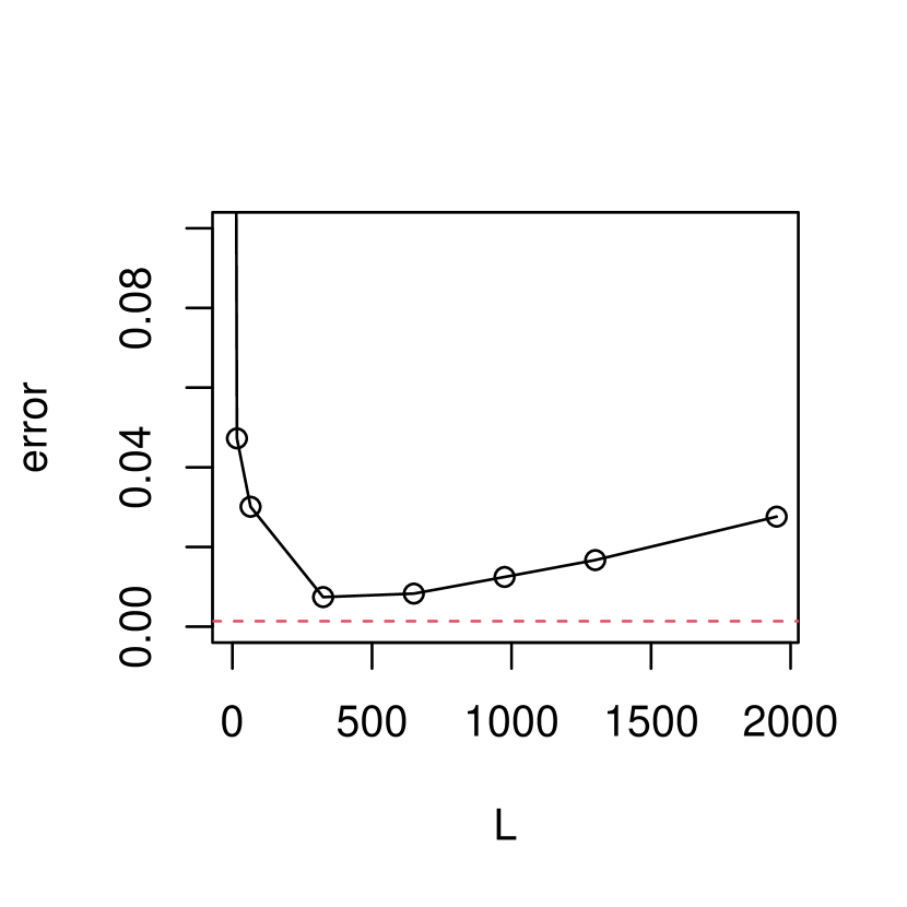
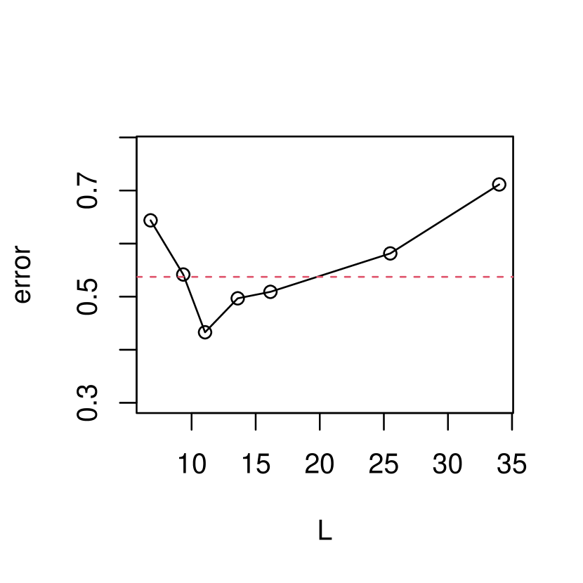
Figure 2: The average tensor estimation errors based on equal spaced intervals under three scenarios of Table 1 with different values of $L$ over 50 independent replications. The red dotted lines are the average estimation errors of the estimate based on adaptively merged intervals. The large error rates in the third panel is due to the much smaller chosen $T$ in the third scenario.

5.2 Real example

We apply the proposed method to analyze a longitudinal network based on the militarized interstate dispute dataset (Palmer et al.,, 2022). The dataset consists of all the major interstate disputes and involved countries during 1895-2014. It can be converted into a longitudinal network with nodes representing all countries ever involved in any dispute over the years. Particularly, we set $dy_{ij}(t)=1$ if country $i$ cooperated with country $j$ in a militarized interstate dispute occurred at time $t$. We keep it as $1$ for the following years until a dispute occurred between themselves, and then $dy_{ij}(t)$ changes to 0 and remains until the next cooperation. This pre-processing step leads to a longitudinal network with $n_{1}=n_{2}=195$ nodes and $110066$ temporal edges, and the time stamps range from 0 to $T=120$ years. We apply the proposed method with $\Delta_{\bm{\delta}}=5$ years and thus $L=24$, where the ranks are set to be $(r_{1},r_{2},r_{3})=(2,2,2)$ following a similar rank selection procedure in Han et al., (2022).

To assess the numeric performance, we randomly split the node pairs into 5 disjoint subsets $\{\mathcal{P}_{p}\}_{p=1}^{5}$. For each $p$, we obtain the estimated tensor $\widehat{\mathcal{M}}^{(p)}$ on $\mathcal{P}_{-p}=[n_{1}]\times[n_{2}]\backslash\mathcal{P}_{p}$, and validate the estimation accuracy on $\mathcal{P}_{p}$ in each small interval by,

$$\text{err}^{(p)}=\frac{\|(\mathcal{T}-\widehat{\mathcal{Y}}^{(p)})\circ{\bm{1}}_{\mathcal{P}_{p}}\|_{F}}{\|\mathcal{T}\circ{\bm{1}}_{\mathcal{P}_{p}}\|_{F}},$$

where $\mathcal{T}=(\mathcal{T}_{ij})_{n_{1}\times n_{2}}$ and $\widehat{\mathcal{Y}}^{(p)}\in\mathbb{R}^{n_{1}\times n_{2}}$ contain the true and estimated numbers of temporal edges for each node pair $(i,j)$, ${\bm{1}}_{\mathcal{P}_{p}}\in\mathbb{R}^{n_{1}\times n_{2}}$ is the indicator matrix for $\mathcal{P}_{p}$, and $\circ$ denotes the matrix Hadamard product. Then, the testing error is calculated as $\text{err}=\sum_{p=1}^{5}\text{err}^{(p)}/5$. For AM($\widehat{K}$), $\widehat{\mathcal{Y}}^{(p)}_{\widehat{\bm{\eta}}}$ is obtained by $(\widehat{\mathcal{Y}}_{\widehat{\bm{\eta}}}^{(p)})_{ij}=\sum_{k=1}^{\widehat{K}}\lambda_{0}\exp((\widehat{\mathcal{M}}_{\widehat{\bm{\eta}}}^{(p)})_{ijk})(\widehat{\eta}_{k}-\widehat{\eta}_{k-1})$, whereas $(\widehat{\mathcal{Y}}_{\bm{\delta}}^{(p)})_{ij}=\sum_{l=1}^{\widehat{L}}\lambda_{0}\exp((\widehat{\mathcal{M}}_{\bm{\delta}}^{(p)})_{ijk})(\delta_{l}-\delta_{l-1})$ for ES($L_{\text{opt}}$). The estimates by HOSVD and HOOI are obtained in the same way as in Section 5.1. The averaged testing errors and their standard errors for the competing methods over 50 times replications are provided in Table 4. It is evident that AM($\widehat{K}$) and ES($L$) significantly outperform the spectral methods, and the difference between AM($\widehat{K}$) and ES($L$) is not significant, which is not surprising as $T=120$ is not large enough compared with $n=195$, corresponding to the third scenario in Table 1.

Table 4: The average testing errors and standard errors (in parentheses) for various methods over 50 replications.

AM($\widehat{K}$)	ES(L)	HOSVD	HOOI
0.739(0.037)	0.752(0.087)	1.160(0.002)	1.163(0.002)

Furthermore, the output of AM$(\widehat{K})$ yields that $\widehat{K}=6$ and $\widehat{\bm{\eta}}=(20,45,50,95,105,120)$, and thus the adaptively merged time intervals are 1895-1914, 1915-1939, 1940-1944, 1945-1989, 1990-1999 and 2000-2014. These intervals appear to be closely related with a number of major world-wide events: before WWI, recess between WWI and WWII, WWII, Cold War, the 90s, and the 21st century. The estimated temporal embedding vectors $\{\widehat{\mathbf{w}}_{l,\bm{\delta}}\}_{l=1}^{L}$ are shown in Figure 3, where $\widehat{\mathbf{w}}_{l,\bm{\delta}}$ in different merged time intervals, represented by different colors, are well separated.

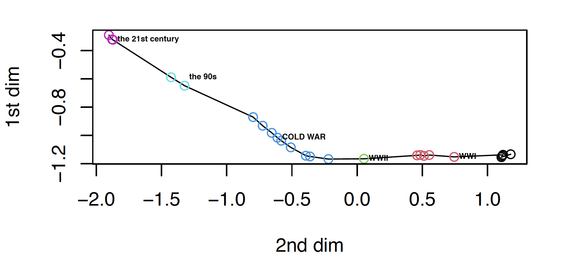
Figure 3: The estimated temporal embedding vectors $\{\widehat{\mathbf{w}}_{l,\bm{\delta}}\}_{l=1}^{9}$, where colors represent different merged time intervals.

It is also interesting to examine the averaged estimation error in each small intervals $[\delta_{l-1},\delta_{l})$, as displayed in Figure 4. Clearly, the estimation errors of AM($\widehat{K}$) are generally smaller than ES($L$) in intervals that do not contain the estimated change points, but more or less comparable in intervals containing the estimated change points. This phenomenon reveals that adaptive merging actually leads to a smaller tensor estimation error than ES($L$) over the time line, while it produces similar errors in those small number of intervals containing the estimated change points, which somehow dominates the tensor estimation errors.

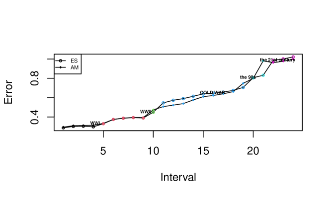
Figure 4: The average estimation errors of AM($\widehat{K}$) and ES($L$) in each of the $L=24$ intervals over 50 replications.

6 Discussion

In this paper, we propose an efficient estimation framework for longitudinal network, leveraging strengths of adaptive network merging, tensor decomposition and point process. A thorough analysis is conducted to quantify the asymptotic behavior of the proposed method, which shows that adaptively network merging leads to substantially improved estimation accuracy compared with existing competitors in literature. The theoretical analysis also provides a guideline for network merging under various scenarios. The advantage of the proposed method is supported in the numerical experiments on both synthetic and real longitudinal networks. The proposed estimation framework can be further extended to incorporate edge-wise or node-wise covariates or employ some more general counting processes, which will be left for future investigation.

Appendix

The proof of Theorem 4 is provided below, whereas other technical proofs are contained in a separate supplementary file.

References

- Aggarwal and Subbian, (2014) Aggarwal, C. and Subbian, K. (2014). Evolutionary network analysis: A survey. ACM Computing Surveys (CSUR), 47:1–36.
- Athreya et al., (2017) Athreya, A., Fishkind, D. E., Tang, M., Priebe, C. E., Park, Y., Vogelstein, J. T., Levin, K., Lyzinski, V., and Qin, Y. (2017). Statistical inference on random dot product graphs: a survey. The Journal of Machine Learning Research, 18:8393–8484.
- Avena-Koenigsberger et al., (2018) Avena-Koenigsberger, A., Misic, B., and Sporns, O. (2018). Communication dynamics in complex brain networks. Nature Reviews Neuroscience, 19:17–33.
- Cai et al., (2022) Cai, J.-F., Li, J., and Xia, D. (2022). Generalized low-rank plus sparse tensor estimation by fast riemannian optimization. Journal of the American Statistical Association, pages 1–17.
- Cranmer and Desmarais, (2011) Cranmer, S. J. and Desmarais, B. A. (2011). Inferential network analysis with exponential random graph models. Political Analysis, 19:66–86.
- (6) De Lathauwer, L., De Moor, B., and Vandewalle, J. (2000a). A multilinear singular value decomposition. SIAM Journal on Matrix Analysis and Applications, 21:1253–1278.
- (7) De Lathauwer, L., De Moor, B., and Vandewalle, J. (2000b). On the best rank-1 and rank- approximation of higher-order tensors. SIAM Journal on Matrix Analysis and Applications, 21:1324–1342.
- De Ruiter et al., (2005) De Ruiter, P. C., Wolters, V., and Moore, J. C. (2005). Dynamic food webs: multispecies assemblages, ecosystem development and environmental change. Elsevier.
- Han et al., (2022) Han, R., Willett, R., and Zhang, A. R. (2022). An optimal statistical and computational framework for generalized tensor estimation. The Annals of Statistics, 50:1–29.
- Hanneke et al., (2010) Hanneke, S., Fu, W., and Xing, E. P. (2010). Discrete temporal models of social networks. Electronic Journal of Statistics, 4:585–605.
- Hao et al., (2013) Hao, N., Niu, Y. S., and Zhang, H. (2013). Multiple change-point detection via a screening and ranking algorithm. Statistica Sinica, 23:1553.
- Hoff et al., (2002) Hoff, P., Raftery, A., and Handcock, M. (2002). Latent space approaches to social network analysis. Journal of the American Statistical Association, 97:1090–1098.
- Holme and Saramäki, (2012) Holme, P. and Saramäki, J. (2012). Temporal networks. Physics Reports, 519:97–125.
- Huang et al., (2023) Huang, S., Weng, H., and Feng, Y. (2023). Spectral clustering via adaptive layer aggregation for multi-layer networks. Journal of Computational and Graphical Statistics, 32:1170–1184.
- Kim et al., (2018) Kim, B., Lee, K. H., Xue, L., and Niu, X. (2018). A review of dynamic network models with latent variables. Statistics Surveys, 12:105.
- Kinne, (2013) Kinne, B. J. (2013). Network dynamics and the evolution of international cooperation. American Political Science Review, 107:766–785.
- Lyu et al., (2021) Lyu, Z., Xia, D., and Zhang, Y. (2021). Latent space model for higher-order networks and generalized tensor decomposition. arXiv preprint arXiv:2106.16042.
- Matias and Miele, (2017) Matias, C. and Miele, V. (2017). Statistical clustering of temporal networks through a dynamic stochastic block model. Journal of the Royal Statistical Society: Series B (Statistical Methodology), 79:1119–1141.
- Matias et al., (2018) Matias, C., Rebafka, T., and Villers, F. (2018). A semiparametric extension of the stochastic block model for longitudinal networks. Biometrika, 105:665–680.
- Niu et al., (2016) Niu, Y. S., Hao, N., and Zhang, H. (2016). Multiple change-point detection: A selective overview. Statistical Science, 31:611–623.
- Palmer et al., (2022) Palmer, G., McManus, R. W., D’Orazio, V., Kenwick, M. R., Karstens, M., Bloch, C., Dietrich, N., Kahn, K., Ritter, K., and Soules, M. J. (2022). The mid5 dataset, 2011–2014: Procedures, coding rules, and description. Conflict Management and Peace Science, 39:470–482.
- Perry and Wolfe, (2013) Perry, P. O. and Wolfe, P. J. (2013). Point process modelling for directed interaction networks. Journal of the Royal Statistical Society: Series B (Statistical Methodology), 75:821–849.
- Perry-Smith and Shalley, (2003) Perry-Smith, J. E. and Shalley, C. E. (2003). The social side of creativity: A static and dynamic social network perspective. Academy of Management Review, 28:89–106.
- Rubin-Delanchy et al., (2022) Rubin-Delanchy, P., Cape, J., Tang, M., and Priebe, C. E. (2022). A statistical interpretation of spectral embedding: The generalised random dot product graph. Journal of the Royal Statistical Society Series B: Statistical Methodology, 84:1446–1473.
- Sewell and Chen, (2015) Sewell, D. K. and Chen, Y. (2015). Latent space models for dynamic networks. Journal of the American Statistical Association, 110:1646–1657.
- Sewell and Chen, (2016) Sewell, D. K. and Chen, Y. (2016). Latent space models for dynamic networks with weighted edges. Social Networks, 44:105–116.
- Sit et al., (2021) Sit, T., Ying, Z., and Yu, Y. (2021). Event history analysis of dynamic networks. Biometrika, 108:223–230.
- Snijders, (2017) Snijders, T. A. (2017). Stochastic actor-oriented models for network dynamics. Annual Review of Statistics and Its Application, 4:343–363.
- Snijders et al., (2010) Snijders, T. A., Koskinen, J., and Schweinberger, M. (2010). Maximum likelihood estimation for social network dynamics. The Annals of Applied Statistics, 4:567.
- Soliman et al., (2022) Soliman, H., Zhao, L., Huang, Z., Paul, S., and Xu, K. S. (2022). The multivariate community hawkes model for dependent relational events in continuous-time networks. In International Conference on Machine Learning, pages 20329–20346. PMLR.
- Ulanowicz, (2004) Ulanowicz, R. E. (2004). Quantitative methods for ecological network analysis. Computational Biology and Chemistry, 28:321–339.
- Voytek and Knight, (2015) Voytek, B. and Knight, R. T. (2015). Dynamic network communication as a unifying neural basis for cognition, development, aging, and disease. Biological Psychiatry, 77:1089–1097.
- (33) Vu, D., Hunter, D., Smyth, P., and Asuncion, A. (2011a). Continuous-time regression models for longitudinal networks. In Shawe-Taylor, J., Zemel, R., Bartlett, P., Pereira, F., and Weinberger, K., editors, Advances in Neural Information Processing Systems, volume 24. Curran Associates, Inc.
- (34) Vu, D. Q., Asuncion, A. U., Hunter, D. R., and Smyth, P. (2011b). Dynamic egocentric models for citation networks. In International Conference on Machine Learning, page 857–864.
- Wainwright, (2019) Wainwright, M. J. (2019). High-dimensional statistics: A non-asymptotic viewpoint, volume 48. Cambridge university press.
- Zhang et al., (2022) Zhang, J., He, X., and Wang, J. (2022). Directed community detection with network embedding. Journal of the American Statistical Association, 117:1809–1819.
- (37) Zhen, Y. and Wang, J. (2023, in press). Community detection in general hypergraph via graph embedding. Journal of the American Statistical Association.