COSMOS-Web: An Overview of the JWST Cosmic Origins Survey

Caitlin M. Casey First two authors are co-first-authors The University of Texas at Austin, 2515 Speedway Blvd Stop C1400, Austin, TX 78712, USA Cosmic Dawn Center (DAWN), Denmark Jeyhan S. Kartaltepe First two authors are co-first-authors Laboratory for Multiwavelength Astrophysics, School of Physics and Astronomy, Rochester Institute of Technology, 84 Lomb Memorial Drive, Rochester, NY 14623, USA Nicole E. Drakos Department of Astronomy and Astrophysics, University of California, Santa Cruz, 1156 High Street, Santa Cruz, CA 95064, USA Maximilien Franco The University of Texas at Austin, 2515 Speedway Blvd Stop C1400, Austin, TX 78712, USA Santosh Harish Laboratory for Multiwavelength Astrophysics, School of Physics and Astronomy, Rochester Institute of Technology, 84 Lomb Memorial Drive, Rochester, NY 14623, USA Louise Paquereau Institut d’Astrophysique de Paris, UMR 7095, CNRS, and Sorbonne Université, 98 bis boulevard Arago, F-75014 Paris, France Olivier Ilbert Aix Marseille Université, CNRS, CNES, LAM, Marseille, France Caitlin Rose Laboratory for Multiwavelength Astrophysics, School of Physics and Astronomy, Rochester Institute of Technology, 84 Lomb Memorial Drive, Rochester, NY 14623, USA Isabella G. Cox Laboratory for Multiwavelength Astrophysics, School of Physics and Astronomy, Rochester Institute of Technology, 84 Lomb Memorial Drive, Rochester, NY 14623, USA James W. Nightingale Department of Physics, Institute for Computational Cosmology, Durham University, South Road, Durham DH1 3LE, UK Brant E. Robertson Department of Astronomy and Astrophysics, University of California, Santa Cruz, 1156 High Street, Santa Cruz, CA 95064, USA John D. Silverman Kavli Institute for the Physics and Mathematics of the Universe (WPI), The University of Tokyo, Kashiwa, Chiba 277-8583, Japan Department of Astronomy, School of Science, The University of Tokyo, 7-3-1 Hongo, Bunkyo, Tokyo 113-0033, Japan Anton M. Koekemoer Space Telescope Science Institute, 3700 San Martin Dr., Baltimore, MD 21218, USA Richard Massey Department of Physics, Centre for Extragalactic Astronomy, Durham University, South Road, Durham DH1 3LE, UK Henry Joy McCracken Institut d’Astrophysique de Paris, UMR 7095, CNRS, and Sorbonne Université, 98 bis boulevard Arago, F-75014 Paris, France Jason Rhodes Jet Propulsion Laboratory, California Institute of Technology, 4800 Oak Grove Drive, Pasadena, CA 91001, USA Hollis B. Akins The University of Texas at Austin, 2515 Speedway Blvd Stop C1400, Austin, TX 78712, USA Natalie Allen Cosmic Dawn Center (DAWN), Denmark Niels Bohr Institute, University of Copenhagen, Jagtvej 128, DK-2200, Copenhagen, Denmark Aristeidis Amvrosiadis Department of Physics, Centre for Extragalactic Astronomy, Durham University, South Road, Durham DH1 3LE, UK Department of Physics, Institute for Computational Cosmology, Durham University, South Road, Durham DH1 3LE, UK Rafael C. Arango-Toro Aix Marseille Université, CNRS, CNES, LAM, Marseille, France Micaela B. Bagley The University of Texas at Austin, 2515 Speedway Blvd Stop C1400, Austin, TX 78712, USA Angela Bongiorno INAF-Observatory of Rome, via Frascati 33, 00074 Monteporzio Catone, Italy Peter L. Capak Cosmic Dawn Center (DAWN), Denmark Niels Bohr Institute, University of Copenhagen, Jagtvej 128, DK-2200, Copenhagen, Denmark Jaclyn B. Champagne Steward Observatory, University of Arizona, 933 N Cherry Ave, Tucson, AZ 85721, USA Nima Chartab The Observatories of the Carnegie Institution for Science, 813 Santa Barbara St., Pasadena, CA 91101, USA Óscar A. Chávez Ortiz The University of Texas at Austin, 2515 Speedway Blvd Stop C1400, Austin, TX 78712, USA Katherine Chworowsky NSF Graduate Research Fellow The University of Texas at Austin, 2515 Speedway Blvd Stop C1400, Austin, TX 78712, USA Kevin C. Cooke Association of Public and Land-grant Universities, 1220 L Street NW, Suite 1000, Washington, DC 20005, USA Olivia R. Cooper NSF Graduate Research Fellow The University of Texas at Austin, 2515 Speedway Blvd Stop C1400, Austin, TX 78712, USA Behnam Darvish Department of Physics and Astronomy, University of California, Riverside, 900 University Avenue, Riverside, CA 92521, USA Xuheng Ding Kavli Institute for the Physics and Mathematics of the Universe (WPI), The University of Tokyo, Kashiwa, Chiba 277-8583, Japan Andreas L. Faisst Caltech/IPAC, 1200 E. California Blvd., Pasadena, CA 91125, USA Steven L. Finkelstein The University of Texas at Austin, 2515 Speedway Blvd Stop C1400, Austin, TX 78712, USA Seiji Fujimoto NASA Hubble Fellow The University of Texas at Austin, 2515 Speedway Blvd Stop C1400, Austin, TX 78712, USA Fabrizio Gentile University of Bologna - Department of Physics and Astronomy “Augusto Righi” (DIFA), Via Gobetti 93/2, I-40129 Bologna, Italy INAF, Osservatorio di Astrofisica e Scienza dello Spazio, Via Gobetti 93/3, I-40129, Bologna, Italy Steven Gillman Cosmic Dawn Center (DAWN), Denmark DTU-Space, Technical University of Denmark, Elektrovej 327, DK-2800 Kgs. Lyngby, Denmark Katriona M. L. Gould Cosmic Dawn Center (DAWN), Denmark Niels Bohr Institute, University of Copenhagen, Jagtvej 128, DK-2200, Copenhagen, Denmark Ghassem Gozaliasl Department of Physics, University of Helsinki, P.O. Box 64, FI-00014 Helsinki, Finland Christopher C. Hayward Center for Computational Astrophysics, Flatiron Institute, 162 Fifth Avenue, New York, NY 10010, USA Qiuhan He Department of Physics, Institute for Computational Cosmology, Durham University, South Road, Durham DH1 3LE, UK Shoubaneh Hemmati Caltech/IPAC, 1200 E. California Blvd., Pasadena, CA 91125, USA Michaela Hirschmann Institute of Physics, GalSpec, Ecole Polytechnique Federale de Lausanne, Observatoire de Sauverny, Chemin Pegasi 51, 1290 Versoix, Switzerland INAF, Astronomical Observatory of Trieste, Via Tiepolo 11, 34131 Trieste, Italy Knud Jahnke Max Planck Institute for Astronomy, Königstuhl 17, D-69117 Heidelberg, Germany Shuowen Jin Cosmic Dawn Center (DAWN), Denmark DTU-Space, Technical University of Denmark, Elektrovej 327, DK-2800 Kgs. Lyngby, Denmark Ali Ahmad Khostovan Laboratory for Multiwavelength Astrophysics, School of Physics and Astronomy, Rochester Institute of Technology, 84 Lomb Memorial Drive, Rochester, NY 14623, USA Vasily Kokorev Kapteyn Astronomical Institute, University of Groningen, PO Box 800, 9700 AV Groningen, The Netherlands Erini Lambrides NPP Fellow NASA Goddard Space Flight Center, Code 662, Greenbelt, MD, 20771, USA Clotilde Laigle Institut d’Astrophysique de Paris, UMR 7095, CNRS, and Sorbonne Université, 98 bis boulevard Arago, F-75014 Paris, France Rebecca L. Larson NSF Graduate Research Fellow The University of Texas at Austin, 2515 Speedway Blvd Stop C1400, Austin, TX 78712, USA Gene C. K. Leung The University of Texas at Austin, 2515 Speedway Blvd Stop C1400, Austin, TX 78712, USA Daizhong Liu Max-Planck-Institut für Extraterrestrische Physik (MPE), Giessenbachstr. 1, D-85748 Garching, Germany Tobias Liaudat Université Paris-Saclay, Université Paris Cité, CEA, CNRS, AIM, 91191, Gif-sur-Yvette, France Arianna S. Long NASA Hubble Fellow The University of Texas at Austin, 2515 Speedway Blvd Stop C1400, Austin, TX 78712, USA Georgios Magdis Cosmic Dawn Center (DAWN), Denmark DTU-Space, Technical University of Denmark, Elektrovej 327, DK-2800 Kgs. Lyngby, Denmark Niels Bohr Institute, University of Copenhagen, Jagtvej 128, DK-2200, Copenhagen, Denmark Guillaume Mahler Department of Physics, Centre for Extragalactic Astronomy, Durham University, South Road, Durham DH1 3LE, UK Department of Physics, Institute for Computational Cosmology, Durham University, South Road, Durham DH1 3LE, UK Vincenzo Mainieri European Southern Observatory, Karl-Schwarzschild-Straße 2, D-85748 Garching bei München, Germany Sinclaire M. Manning NASA Hubble Fellow Department of Astronomy, University of Massachusetts Amherst, 710 N Pleasant Street, Amherst, MA 01003, USA Claudia Maraston Institute of Cosmology and Gravitation, University of Portsmouth, Dennis Sciama Building, Burnaby Road, Portsmouth, PO13FX, UK Crystal L. Martin Department of Physics, University of California, Santa Barbara, Santa Barbara, CA 93109, USA Jacqueline E. McCleary Department of Physics, Northeastern University, 360 Huntington Ave, Boston, MA 02115, USA Jed McKinney The University of Texas at Austin, 2515 Speedway Blvd Stop C1400, Austin, TX 78712, USA Conor J. R. McPartland Cosmic Dawn Center (DAWN), Denmark Niels Bohr Institute, University of Copenhagen, Jagtvej 128, DK-2200, Copenhagen, Denmark Bahram Mobasher Department of Physics and Astronomy, University of California, Riverside, 900 University Avenue, Riverside, CA 92521, USA Rohan Pattnaik Laboratory for Multiwavelength Astrophysics, School of Physics and Astronomy, Rochester Institute of Technology, 84 Lomb Memorial Drive, Rochester, NY 14623, USA Alvio Renzini Istituto Nazionale di Astrofisica (INAF), Osservatorio Astronomico di Padova, Vicolo dell’Osservatorio 5, 35122, Padova, Italy R. Michael Rich Department of Physics and Astronomy, UCLA, PAB 430 Portola Plaza, Box 951547, Los Angeles, CA 90095, USA David B. Sanders Institute for Astronomy, University of Hawai’i at Manoa, 2680 Woodlawn Drive, Honolulu, HI 96822, USA Zahra Sattari Department of Physics and Astronomy, University of California, Riverside, 900 University Avenue, Riverside, CA 92521, USA The Observatories of the Carnegie Institution for Science, 813 Santa Barbara St., Pasadena, CA 91101, USA Diana Scognamiglio Argelander-Institut für Astronomie, Auf dem Hügel 71, D-53121, Bonn, Germany Nick Scoville Astronomy Department, California Institute of Technology, 1200 E. California Blvd, Pasadena, CA 91125, USA Kartik Sheth NASA Headquarters, 300 Hidden Figures Way, SE, Mary W. Jackson NASA HQ Building, Washington, DC 20546, USA Marko Shuntov Institut d’Astrophysique de Paris, UMR 7095, CNRS, and Sorbonne Université, 98 bis boulevard Arago, F-75014 Paris, France Martin Sparre Institut für Physik und Astronomie, Universität Potsdam, Karl-Liebknecht-Str. 24/25, 14476 Golm, Germany Leibniz-Institut für Astrophysik Potsdam (AIP), An der Sternwarte 16, 14482 Potsdam, Germany Tomoko L. Suzuki Kavli Institute for the Physics and Mathematics of the Universe (WPI), The University of Tokyo, Kashiwa, Chiba 277-8583, Japan Margherita Talia University of Bologna - Department of Physics and Astronomy “Augusto Righi” (DIFA), Via Gobetti 93/2, I-40129 Bologna, Italy INAF, Osservatorio di Astrofisica e Scienza dello Spazio, Via Gobetti 93/3, I-40129, Bologna, Italy Sune Toft Cosmic Dawn Center (DAWN), Denmark Niels Bohr Institute, University of Copenhagen, Jagtvej 128, DK-2200, Copenhagen, Denmark Benny Trakhtenbrot School of Physics and Astronomy, Tel Aviv University, Tel Aviv 69978, Israel C. Megan Urry Physics Department and Yale Center for Astronomy & Astrophysics, Yale University, PO Box 208120, CT 06520, USA Francesco Valentino Cosmic Dawn Center (DAWN), Denmark Niels Bohr Institute, University of Copenhagen, Jagtvej 128, DK-2200, Copenhagen, Denmark Brittany N. Vanderhoof Laboratory for Multiwavelength Astrophysics, School of Physics and Astronomy, Rochester Institute of Technology, 84 Lomb Memorial Drive, Rochester, NY 14623, USA Eleni Vardoulaki Thüringer Landessternwarte, Sternwarte 5, 07778 Tautenburg, Germany John R. Weaver Department of Astronomy, University of Massachusetts Amherst, 710 N Pleasant Street, Amherst, MA 01003, USA Katherine E. Whitaker Department of Astronomy, University of Massachusetts Amherst, 710 N Pleasant Street, Amherst, MA 01003, USA Cosmic Dawn Center (DAWN), Denmark Stephen M. Wilkins Astronomy Centre, University of Sussex, Falmer, Brighton BN1 9QH, UK Institute of Space Sciences and Astronomy, University of Malta, Msida MSD 2080, Malta Lilan Yang Kavli Institute for the Physics and Mathematics of the Universe (WPI), The University of Tokyo, Kashiwa, Chiba 277-8583, Japan Jorge A. Zavala National Astronomical Observatory of Japan, 2-21-1 Osawa, Mitaka, Tokyo 181-8588, Japan

Abstract

We present the survey design, implementation, and outlook for COSMOS-Web, a 255 hour treasury program conducted by the James Webb Space Telescope in its first cycle of observations. COSMOS-Web is a contiguous 0.54 deg² NIRCam imaging survey in four filters (F115W, F150W, F277W, and F444W) that will reach 5 $\sigma$ point source depths ranging $\sim$ 27.5–28.2 magnitudes. In parallel, we will obtain 0.19 deg² of MIRI imaging in one filter (F770W) reaching 5 $\sigma$ point source depths of $\sim$ 25.3–26.0 magnitudes. COSMOS-Web will build on the rich heritage of multiwavelength observations and data products available in the COSMOS field. The design of COSMOS-Web is motivated by three primary science goals: (1) to discover thousands of galaxies in the Epoch of Reionization ( $6\lower 2.15277pt\hbox{$\;\buildrel<\over{\sim}\;$}z\lower 2.15277pt\hbox{$\;\buildrel<\over{\sim}\;$}11$ ) and map reionization’s spatial distribution, environments, and drivers on scales sufficiently large to mitigate cosmic variance, (2) to identify hundreds of rare quiescent galaxies at $z>4$ and place constraints on the formation of the Universe’s most massive galaxies ( $M_{\star}>10^{10}$ M_⊙), and (3) directly measure the evolution of the stellar mass to halo mass relation using weak gravitational lensing out to $z\sim 2.5$ and measure its variance with galaxies’ star formation histories and morphologies. In addition, we anticipate COSMOS-Web’s legacy value to reach far beyond these scientific goals, touching many other areas of astrophysics, such as the identification of the first direct collapse black hole candidates, ultracool sub-dwarf stars in the Galactic halo, and possibly the identification of $z>10$ pair-instability supernovae. In this paper we provide an overview of the survey’s key measurements, specifications, goals, and prospects for new discovery.

1 Introduction

Designed to peer into the abyss, extragalactic deep fields have pushed the limits of our astronomical observations as far and as faint as possible. The first of these deep fields imaged with the Hubble Space Telescope (the medium deep survey and the Hubble Deep Field North, or HDF-N; Griffiths et al., 1996; Williams et al., 1996) pushed three magnitudes fainter than could be reached with ground-based telescopes at the time. Their data revealed a surprisingly high density of distant galaxies, well above expectation. This surprise was due to high-redshift galaxies’ elevated surface brightness relative to nearby galaxies, likely caused by their overall higher star formation rates. It quickly became clear that “the Universe at high redshift looks rather different than it does at the current epoch” (Williams et al., 1996).

This unexpected richness found in these first deep fields marked a major shift in astronomy’s approach to high-redshift extragalactic science, moving from specialized case studies scattered about the sky and instead placing more emphasis on statistical studies using multiwavelength observations in a few deep fields where the density of information was very high. Such a transformation had a major role in leveling access to the high-redshift Universe for a wide array of researchers worldwide, regardless of their individual access to astronomical observatories. Several other deep fields were pursued in short order after the HDF-N with Hubble, the other Great Observatories, and ancillary observations across the spectrum from the ground and space (e.g., the HDF-S, CDFN and CDFS, GOODS-N and GOODS-S, and the HUDF; Williams et al., 2000; Brandt et al., 2000; Giacconi et al., 2002; Giavalisco et al., 2004; Beckwith et al., 2006), complementing each other in depth and area and providing crucial insight into the diversity of galaxies from the faintest, lowest-mass systems to the brightest and most rare.

In parallel to the effort to push deep over narrow fields of view, another experiment with Hubble transformed our understanding of large scale structure (LSS) at high redshifts by mapping a contiguous two square degree area of the sky, $\sim$ 20 times larger than all other deep fields of the time combined. Through its large area and statistical samples (resolving over 2 $\times 10^{6}$ galaxies from $0<z<6$ ), the Cosmic Evolution Survey (COSMOS; Scoville et al., 2007) allowed the first in-depth studies linking the formation and evolution of galaxies to their larger cosmic environments across 93% of cosmic time. By virtue of its large area, COSMOS probed a volume significantly larger than that of “pencil-beam” deep fields and thus substantially minimized uncertainties of key extragalactic measurements from cosmic variance. In addition, the diverse array of multiwavelength observations gathered in the COSMOS field (Capak et al., 2007; Ilbert et al., 2010; Laigle et al., 2016; Weaver et al., 2022a) made it possible to carry out a suite of ambitious survey efforts and understand the distribution of large scale structure at early cosmic epochs (Scoville et al., 2013; Darvish et al., 2015).

Deep field images of the distant Universe – from the deepest, Hubble Ultra Deep Field (HUDF), to the widest, COSMOS – have transformed into rich laboratories for testing hypotheses about the formation and evolution of galaxies through time. These hypotheses initially encompassed the first basic cosmological models and ideas regarding the evolution of galaxy structure. Thanks to the addition of multiwavelength observations in these deep fields, they expanded to include hypotheses about the formation of supermassive black holes, the richness of galaxies’ interstellar media, the assembly of gas in and around galaxies, and the structure of large dark matter haloes.

These deep fields, initially motivated by Hubble but substantially enhanced with a rich suite of ancillary ground-based and space-based data, have deepened our understanding of the evolution of galaxies across cosmic time. They pushed the horizon of the distant Universe into the first billion years, a time marking the last major phase change of the Universe itself from a neutral to an ionized medium (known as the Epoch of Reionization, or EoR, at $z\lower 2.15277pt\hbox{$\;\buildrel>\over{\sim}\;$}6$ , e.g., Stanway et al., 2003; Bunker et al., 2003; Bouwens et al., 2003, 2006; Dickinson et al., 2004). They also enabled the detailed study of galaxy morphologies (e.g., Abraham et al., 1996; Lowenthal et al., 1997; Conselice et al., 2000; Lotz et al., 2006; Scarlata et al., 2007), stellar mass growth (e.g., Sawicki & Yee, 1998; Brinchmann & Ellis, 2000; Papovich et al., 2001), the impact of local environment (e.g., Balogh et al., 2004; Kauffmann et al., 2004; Christlein & Zabludoff, 2005; Cooper et al., 2008; Scoville et al., 2013), the distribution of dark matter across the cosmic web (e.g., Natarajan et al., 1998; Mandelbaum et al., 2006; Massey et al., 2007a; Leauthaud et al., 2007, 2011), as well as the discovery of the tight relationship between galaxies stellar masses and star formation rates (e.g., the galaxies’ “star-forming main sequence,” Daddi et al., 2007; Noeske et al., 2007; Elbaz et al., 2007).

However, due to the expansion of the Universe, the next leap forward required observations in the near-infrared (NIR) part of the spectrum. That came with the installation of the WFC3 camera on Hubble during the 2009 servicing mission. WFC3 expanded Hubble’s deep field capabilities into the NIR at similar depths as was previously achieved in the optical, enabling a tenfold increase in the number of candidate galaxies identified beyond $z\lower 2.15277pt\hbox{$\;\buildrel>\over{\sim}\;$}6$ (Robertson et al., 2015; Bouwens et al., 2015; Finkelstein et al., 2015; Finkelstein, 2016; Stark, 2016), from a few hundred to a few thousand as well as the study of galaxies’ rest-frame optical light out to $z\sim 3$ (e.g., Wuyts et al. 2011; Lee et al. 2013; van der Wel et al. 2014; Kartaltepe et al. 2015a). The Cosmic Assembly Near-infrared Deep Extragalactic Legacy Survey (CANDELS; Grogin et al., 2011; Koekemoer et al., 2011) was particularly pioneering as it imaged portions of five of the key deep fields (GOODS-N, GOODS-S, UDS, EGS, and COSMOS) with the F125W and F160W filters over a total area of $\sim$ 800 arcmin².

The successful launch of the James Webb Space Telescope (JWST) now marks a new era for studying the infrared Universe and the distant cosmos. With six times the collecting area of Hubble and optimized for observations in the near- and mid-infrared, JWST is currently providing images with greater depth and spatial resolution than previously possible. This is beginning to enable a substantial improvement in our understanding of galaxy evolution during the first few hundred million years (the epoch of cosmic dawn, $z\lower 2.15277pt\hbox{$\;\buildrel>\over{\sim}\;$}6$ ) to the peak epoch of galaxy assembly (known as cosmic noon, $1\leq z\leq 3$ ). Given the tremendous legacy value of the deep fields imaged by the Great Observatories, several JWST deep fields have been planned for the observatory’s first year of observations. The largest program among these, in both area on the sky and total prime time allocation, is the COSMOS-Web¹¹1 This survey was originally named COSMOS-Webb, as a combination of the telescope name and in reference to the cosmic web, but later renamed to emphasize the scientific goal of mapping the cosmic web on large scales as well as to be inclusive and supportive to members of the LGBTQIA+ community. Survey (PIs: Kartaltepe & Casey), for which this paper provides an overview.

Refer to caption — Figure 1: A map of the COSMOS-Web tiling pattern embedded within the Hubble ACS F814W mosaic of the COSMOS field (Scoville et al., 2007; Koekemoer et al., 2007). The mosaic consists of 152 visits where NIRCam serves as the primary instrument (long wavelength detector coverage shown in blue) with MIRI in parallel (shown in orange). The entire NIRCam mosaic is centered on the position $\alpha$ =10:00:27.9, $\delta$ = $+$ 02:12:03.5 and is 41.5 arcminutes (in the east-west direction) $\times$ 46.6 arcminutes (in the north-south direction) in size. The entire mosaic has an average position angle of 110^∘, with individual visit PAs equal to 293^o in the northern half and 107^∘ in the southern half. Three visits required slightly different position angles due to availability of guide stars; this includes the lone northern-most MIRI tile. The detailed coordinates and position angles of each visit are provided in the Appendix, § A.

COSMOS-Web was designed to bridge deep pencil-beam surveys from Hubble with shallower wide-area surveys, such as those that will be made possible by facilities like the future Roman Space Telescope (Akeson et al., 2019) and Euclid (Euclid Collaboration et al., 2022). With its unique combination of contiguous area and depth, COSMOS-Web will enable countless scientific investigations by the broader community. It will forge the detection of thousands of galaxies beyond $z>6$ , while also mapping the environments of those discoveries on scales larger than the largest coherent structures in the cosmic web on $\;\buildrel>\over{\sim}\;$ 10 Mpc scales. It will identify hundreds of the rarest quiescent galaxies in the early Universe ( $z>4$ ) and place constraints on the formation mechanisms of the most massive galaxies. It will also directly measure the evolution of the stellar mass to halo mass relation (SMHR) out to $z\sim 2.5$ as a function of various galaxy properties using weak lensing measurements to estimate halo mass.

This paper describes the motivation for the COSMOS-Web survey as well as the program’s design, providing an initial overview of what is to come as the data are collected, processed, and analyzed. Section 2 presents the detailed observational design of the survey and Section 3 briefly describes the context of COSMOS-Web among other deep fields planned for the first year of JWST observations. Section 4 presents the scientific motivation of the survey as the drivers for the observational design. In Section 5, we share other possible investigations and predictions for what will be made possible by COSMOS-Web, beyond the main science goals. We summarize our outlook for the survey in section 6. Throughout this paper, we use AB magnitudes (Oke & Gunn, 1983), assume a Chabrier stellar initial mass function (Chabrier, 2003), and a concordance cosmology with $H_{0}=70~{}{\rm km~{}s^{-1}~{}Mpc^{-1}}$ and $(\Omega_{tot},\Omega_{\Lambda},\Omega_{m})=(1,0.7,0.3)$ .

2 Observational Design

The observational design of the COSMOS-Web survey is motivated by the requirements of the primary science drivers described in §4 while also striving to maximize value for the broader community across a wide range of science topics, described in part in § 5. Here we describe the detailed layout of the COSMOS-Web survey and provide more detailed motivation for the design when discussing the science goals in § 4.

Table 1: Summary of COSMOS-Web NIRCam Survey Depth

No. of NIRCam	Total NIRCam	SW Area	F115W Depth	F150W Depth	LW Area	F277W Depth	F444W Depth
Exposures	Exp. Time (s)	(arcmin²)	(5 $\sigma$ )	(5 $\sigma$ )	(arcmin²)	(5 $\sigma$ )	(5 $\sigma$ )
1	257.68	71.3	26.87	27.14	17.8	27.71	27.61
2	515.36	991.6	27.13	27.35	978.0	27.99	27.83
3	773.05	60.0	27.26	27.50	24.4	28.12	27.94
4	1030.73	805.2	27.45	27.66	904.3	28.28	28.17

Note. — Depths quoted are average 5 $\sigma$ point source depths calculated within 0 $\farcs$ 15 radius apertures on data from our first epoch of observations without application of aperture corrections.

Table 2: Summary of COSMOS-Web MIRI Survey Depth

No. of MIRI	Total MIRI	Area Covered	F770W Depth
Exposures	Exp. Time (s)	(arcmin²)	(5 $\sigma$ )
2	527.26	80.5	25.33
4	1054.52	430.4	25.70
6	1581.77	30.8	25.76
8	2109.03	146.1	25.98

Note. — Depths quoted are average 5 $\sigma$ point source depths calculated within 0 $\farcs$ 3 radius apertures on data from our first epoch of observations, without application of aperture corrections.

2.1 Description of Observations

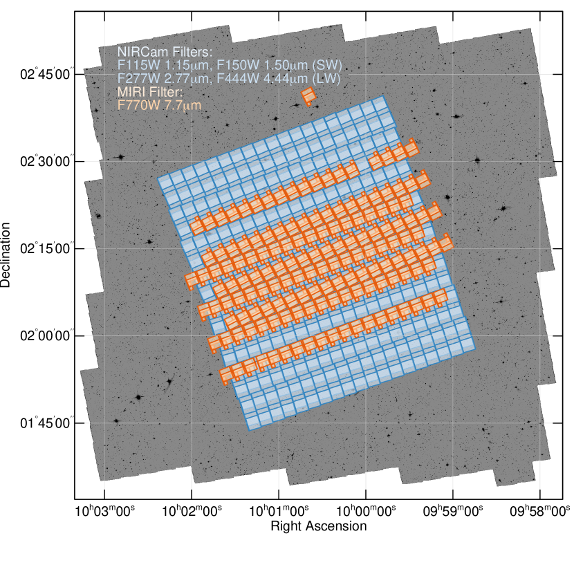
COSMOS-Web consists of one large contiguous 0.54 deg² NIRCam (Rieke et al., 2022) mosaic conducted in four filters (F155W, F150W, F277W, and F444W) with single filter (F770W) MIRI (Wright et al., 2022) imaging observations obtained in parallel over a total non-contiguous area of 0.19 deg². The NIRCam mosaic is spatially distributed as a 41.5 ${}^{\prime}\times$ 46.6^′ rectangle at an average position angle of 110^∘; the shorter side of the mosaic is primarily oriented in the east-west direction. The center of the mosaic is at $\alpha$ =10:00:27.92, $\delta$ = $+$ 02:12:03.5 and is comprised of 152 separate visits (where each visit observes a single tile in the mosaic²²2A single ‘visit’ is a JWST observation acquired in one block of continuously scheduled time.) arranged in a 19 $\times$ 8 grid. The coverage of these visits overlaid on the COSMOS Hubble F814W imaging is shown in Figure 1.

Each individual visit is comprised of eight separate exposures of $\sim$ 257 seconds each, split into two separate executions of the 4TIGHT dither pattern at the same position in the mosaic. Each 4TIGHT dither pattern contains four individual integrations; an illustration of this dither pattern in one standalone visit and embedded in the larger mosaic is shown in Figure 2. The first 4TIGHT dither executes two NIRCam filters – F115W at short wavelengths (SW) and F277W at long wavelengths (LW) – and the MIRI F770W filter in parallel. The second execution of the 4TIGHT dither switches NIRCam filters – to F150W in SW and F444W in LW – yet keeps the same MIRI filter, F770W, for added depth.

The northern half of the mosaic is observed at one position angle, 293^∘, while the southern half of the mosaic is observed at another, 107^∘. These position angles are relative to the NIRCam instrument plane and not V3 (which differ by $<$ 1^∘); they are also not exactly a 180^∘ flip from one another. Instead they are staggered by $\pm$ 3^∘ to make scheduling more flexible while maintaining a contiguous mosaic using a slight jigsaw pattern to stitch adjacent visits together. The distribution of half of the mosaic at one position angle and the other half at another also makes it possible to fit most of the MIRI parallel exposures fully within the larger NIRCam mosaic. A few visits required further position angle modification due to limitations in guide star catalog availability at their initially intended angles. The Appendix (§ A) gives detailed information for each individual visit and a table of all visits.

The depth of the NIRCam observations varies based on the number of exposures at any position in the mosaic (see Table 1); of the total 1928 arcmin² ( $\approx$ 0.54 deg²) area in the NIRCam SW mosaic, 71.3 arcmin² ( $\sim$ 3.7%) will be covered with only a single exposure per SW filter, 991.6 arcmin² ( $\sim$ 51.4%) will have two SW exposures, 60.0 arcmin² ( $\sim$ 3.1%) will have three SW exposures, and 805.2 arcmin² ( $\sim$ 41.8%) will have four SW exposures. The NIRCam LW mosaic covers a total area of 1924 arcmin², of which 17.8 arcmin² ( $\sim$ 0.9%) has single exposure depth, 978.0 arcmin² ( $\sim$ 50.8%) has two exposure depth, 24.4 arcmin² ( $\sim$ 1.3%) has three exposure depth, and 904.3 arcmin² ( $\sim$ 47.0%) has four exposure depth. The most deeply exposed portions of the SW mosaic align with the deepest portions of the LW mosaic, though the areas differ slightly based on the differences in detector size and gaps between SW detectors.

Due to the design of the NIRCam mosaic as contiguous, the MIRI parallel observations are not contiguous but are distributed in 152 distinct regions corresponding to the 152 visits. MIRI coverage of each visit has an area of 4.2 arcmin² corresponding to the primary MIRI imager field of view, and 4.5 arcmin² when accounting for the additional area of the Lyot Coronographic Imager³³3During MIRI imaging, the Lyot Coronographic Imager is also exposed using the same filter and optical path of the imager. Modulo the occulting spot and its support structure, the Lyot region provides a small amount of additional survey area for MIRI imaging campaigns. See the JWST User Documentation Page on MIRI Features and Caveats for more details.. Of that area, 0.55 arcmin² (12%) has two MIRI exposures, 2.81 arcmin² (62%) has four, 0.21 arcmin² (5%) has six, and 0.96 arcmin² (21%) has eight MIRI exposures. The total area covered with MIRI in COSMOS-Web is 688 arcmin² or 0.19 deg². Of the 152 MIRI visits, 143 (651 arcmin², 95%) are fully contained within the NIRCam mosaic. Note that MIRI observations from PRIMER (GO #1837) add an additional 53 arcmin² of (deeper) 7.7 $\mu$ m coverage (see § 3 for full details) contained within the NIRCam footprint, bringing the total MIRI coverage in COSMOS from these two Cycle 1 surveys to 742 arcmin².

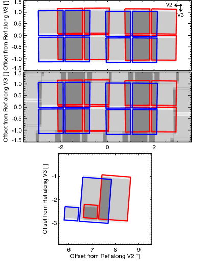
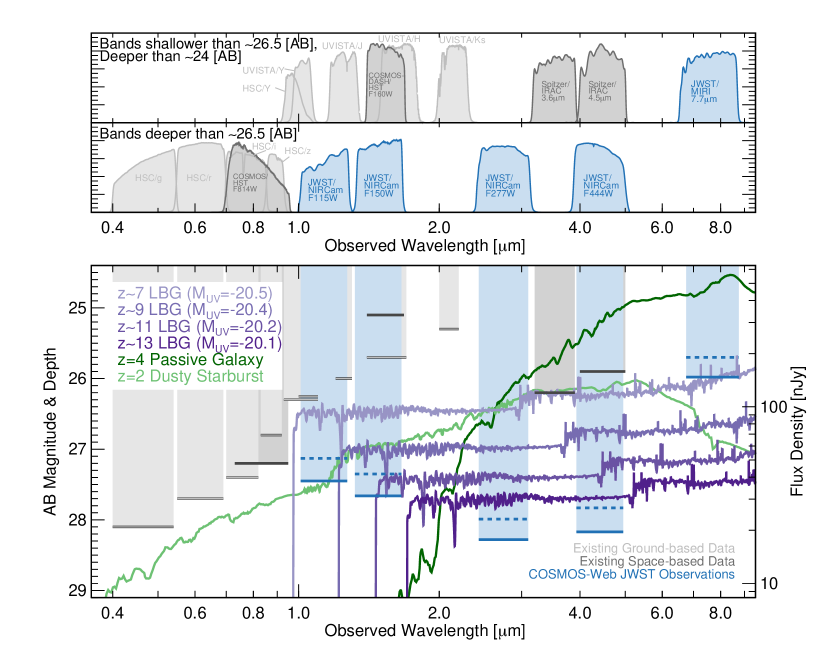
Table 1 summarizes the characteristics of the NIRCam mosaic and the measured depths as a function of number of exposures. The NIRCam depths have been measured using data from the first epoch of COSMOS-Web observations, consisting of six visits (out of the total 152). These data are later described in § 2.7. These are broadly consistent with the expected performance of JWST in-flight (Rigby et al., 2022). These depths correspond to 5 $\sigma$ point sources extracted within 0 $\farcs$ 15 radius circular apertures in each filter without any aperture corrections applied. Table 2 provides a summary for the MIRI exposures; similarly, these depths are measured directly using data from the first epoch of observations in COSMOS-Web using a a 0 $\farcs$ 3 radius circular aperture without aperture correction. We note that the measured MIRI depths are significantly better than expectation from the exposure time calculator. We conducted a number of tests to measure this depth accurately, including a direct comparison of IRAC 8 $\mu$ m flux densities with MIRI 7.7 $\mu$ m flux densities, measurement of depth within empty apertures in individual exposures, as well as measurement of the standard deviation in flux densities for individual sources in individual exposures. All tests give consistent results, showing F770W depths nearly a magnitude deeper than expectation. The depths of the survey as a function of wavelength are shown in Figure 3 relative to other existing datasets available in the COSMOS field.

2.2 Motivation for a Contiguous $\sim$ 0.5 deg² Area

The contiguous, and roughly square, area of COSMOS-Web is driven by two of our primary science objectives. The first is to construct large scale structure density maps at $6<z<10$ to address whether or not the most UV-luminous systems are embedded in overdense structures (see § 4.1 for details). Mapping the large scale environments of our discoveries and mitigating cosmic variance at these epochs (with cosmic variance less than 10%, i.e., $\sigma_{v}^{2}<0.10$ ) requires contiguous solid angles larger than the expected size of reionization bubbles at these redshifts (Behroozi et al., 2019), $>$ 0.3-0.4 deg². Our 0.54 deg² program allows for some uncertainty in the scale of these reionization bubbles, as some simulations see bubbles extend on 40^′ scales (D’Aloisio et al., 2018; Thélie et al., 2022). Our NIRCam mosaic maps to $\sim$ (114 Mpc)² between $6<z<8$ and $\sim$ (122 Mpc)² between $8<z<10$ projected on the sky at these epochs. We describe more about the expected cosmic variance in COSMOS-Web in § 2.6.

The second scientific driver for our contiguous area is the coherence we can achieve for the weak lensing measurement of galaxies’ halo masses on scales $\;\buildrel<\over{\sim}\;$ 10 Mpc in order to place constraints on the SMHR out to $z\sim 2.5$ (see § 4.3 for details). This requires at least $\sim 5$ dark matter halo scale lengths ( $\sim 3$ proper Mpc across each) of contiguous coverage, for which our survey will provide $\sim 10\times 10$ dark matter scale lengths to boost the signal-to-noise and allow splitting by galaxy type and by mass (Wechsler & Tinker, 2018; Wang et al., 2018a; Debackere et al., 2020; Shuntov et al., 2022). Several smaller non-contiguous areas (of order 0.05 deg²) would render the SMHR measurement and calibration of cosmological models severely hindered.

2.3 Field on the Sky

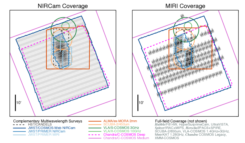
The COSMOS field was chosen for these observations for several reasons. First, the existing HST/ACS F814W coverage (Koekemoer et al., 2007) provides crucial value to our science goals of detecting galaxies beyond $z>6$ using [F814W]-[F115W] colors. Second, COSMOS has the widest deep ancillary data coverage from X-ray to radio wavelengths (Ilbert et al., 2013; Laigle et al., 2016; Weaver et al., 2022a). Third, it is an equatorial field ( $\alpha=150^{\circ}$ , $\delta=+2^{\circ}$ ), and thus accessible to all major existing and planned future facilities, essential for swift and efficient follow-up of JWST-identified sources. A sampling of the multiwavelength data already available in the COSMOS-Web footprint is shown in Figure 4.

Additionally, COSMOS has been selected or is a likely candidate to be a deep calibration field for future key projects including Euclid, the Roman Space Telescope, and the Vera Rubin Observatory LSST project. Over 250,000 spectra have been taken of $>$ 100,000 unique objects in the COSMOS field at $0<z<7$ (A. Khostovan et al. in preparation), including from large surveys such as zCOSMOS (Lilly et al., 2007, 2009), FMOS-COSMOS (Silverman et al., 2015; Kartaltepe et al., 2015b; Kashino et al., 2019), VUDS (Le Fèvre et al., 2015), and many programs using Keck (e.g., Kartaltepe et al. 2010; Capak et al. 2011; Casey et al. 2012; Kriek et al. 2015; Hasinger et al. 2018), greatly enhancing the accuracy of photometric redshifts for all sources in the field. Lastly, the quality of photometric redshifts $\Delta z/(1+z)<0.02$ for galaxies with $i<25$ (Ilbert et al., 2013; Laigle et al., 2016; Weaver et al., 2022a) has facilitated the discovery and analysis of galaxies out to $z\sim 7$ and beyond (Bowler et al., 2017, 2020; Stefanon et al., 2019; Kauffmann et al., 2022). The photometric redshifts will be further improved with the addition of COSMOS-Web (see § 2.5), dramatically improving the accuracy of the weak lensing measurement of galaxies’ halo mass as well as galaxies’ stellar masses and star formation rates across all epochs.

2.4 Filter Optimization

We simulated the effectiveness of many filter combinations to deliver the science objectives described in § 4 and determined that COSMOS-Web should be a four filter NIRCam survey with MIRI imaging conducted in parallel: F115W+F150W in SW, F277W+F444W in LW, and F770W with MIRI. Reionization science drives the choice of F115W and F150W to maximize coverage of the observed wavelength of a Lyman break from $6<z<13$ ; we plan EoR source selection using a hybrid photometric redshift and dropout approach ( $z\sim\,6-7$ galaxies drop out in HST-F814W, while $z\sim\,8-10$ galaxies drop out in the F115W filter, and $z>12$ will drop out in F150W). Weak lensing objectives are less sensitive to filter choice but benefit from tremendous depth in the NIR by increasing the background source density; we expect $>$ 10 galaxies per arcmin² at $z>4$ with measurable shapes, in other words, those found above a 15 $\sigma$ detection threshold. We calculate the on-sky source density of galaxies above certain apparent magnitude thresholds from existing measurements of galaxy luminosity functions from $0<z<10$ (e.g., Arnouts et al., 2005; Bouwens et al., 2015; Finkelstein et al., 2015). Indeed, preliminary simulations show that galaxies at the 15 $\sigma$ shape-detection threshold, F277W $\sim$ 26.8, with $R_{\rm eff}\lower 2.15277pt\hbox{$\;\buildrel<\over{\sim}\;$}\,0\farcs 3\ (\approx$ 2–3 kpc), are recovered without bias introduced from the JWST point spread function (PSF; Liaudat & Scognamiglio et al., in preparation). We find F277W+F444W to be the most advantageous LW filter combination to improve the quality of photometric redshifts and mitigate lower redshift contaminants (more details discussed in § 4.1). The F444W filter is particularly useful for measuring the rest-frame optical morphologies of galaxies at $z>4$ , (e.g., Kartaltepe et al. 2022) and the rest-frame near-infrared morphologies of lower redshift galaxies (e.g., Guo et al. 2022). The LW filters will be useful for the identification of very red $z=4-6$ quiescent galaxies and measuring their mass surface densities and morphologies at high signal-to-noise.

The choice of F770W for the MIRI parallel exposures is motivated by the need to constrain reliable stellar masses for $z>4$ massive systems. F770W is roughly matched to the Spitzer 8.0 $\mu$ m filter (which has much shallower data in COSMOS; Sanders et al., 2007). F770W data will provide a factor of 50 $\times$ improvement in depth relative to Spitzer 8.0 $\mu$ m and a factor of 7.6 $\times$ improvement in the beam size, thus opening up detections to the $z>4$ universe. Our MIRI data will cover an area $\sim$ 3.5 $\times$ larger than all other planned JWST MIRI deep fields from Cycle 1 combined (see § 3), making it particularly sensitive to rare, bright objects. F770W optimizes both sensitivity and the uniqueness of longer rest-frame wavelengths for high redshift galaxies. Longer wavelength filters would reduce the sensitivity by 10–30 $\times$ , and F560W does not provide a sufficient lever arm from F444W to measure high- $z$ galaxy stellar masses.

2.5 Precision of Photometric Redshifts

A crucial aspect of the design of COSMOS-Web was the selection of filters, largely driven by finding the most reliable selection of EoR sources from $6<z<11$ . We generated an empirical light cone of mock galaxies, populating it with galaxies following the galaxy luminosity function from the local Universe to $z\sim 4$ from Arnouts et al. (2005); from $z\sim 4-10$ , galaxies are drawn from the UV luminosity functions of Bouwens et al. (2015). From $z\sim 10-12$ , the Bouwens et al. luminosity functions are extrapolated by fixing $M_{\star}$ and extrapolating trends in $\Phi_{\star}$ and $\alpha$ measured at lower redshift (i.e., higher redshifts have lower densities and steeper faint-end slopes).

Once the on-sky density of galaxies (as a function of rest-frame UV absolute magnitude, $M_{\rm UV}$ ) is set, we assign a variety of spectral energy distributions (SEDs) to each galaxy. Given the focus on reliability of EoR targets, the SEDs we generate were of somewhat limited scope, focusing on three families of templates from Maraston (2005) with 61 ages for each. The primary difference between templates is the star-forming timescale, with exponentially declining star-formation histories of 0.25, 1, and 10 Gyr. Three attenuations were used with $E(B-V)=0,\ 0.05$ , and $0.1$ (not including very reddened sources). Both nebular line emission and IGM opacity (Madau, 1995) were included. The choice of SED for a given galaxy was then assigned using a uniform distribution (with an allowable star-formation timescale). While there are clear limitations to this idealized, empirical calibration sample – such as the lack of more diverse SEDs, a mass- or redshift-weighted method of assigning SEDs, or using a wider set of templates to fit the ensuing photometric redshifts – it can still provide a useful first pass at our photometric redshift precision, particularly for newly-discovered faint galaxies within the EoR.

Noise is added to the mock observations according to the depth in each filter (to the greatest depth as quoted in Tables 1 and 2). Similarly, known noise characteristics of existing ground-based data have been added to the galaxies’ mock photometry (details of those observations are provided by Weaver et al., 2022a). We use this mock sample to diagnose the contamination and precision of our photometric redshifts across all epochs, applying tools we will use for the real dataset. Specifically, here we use the LePhare SED fitting code to derive photometric redshifts (Arnouts et al., 2002; Ilbert et al., 2006), as implemented for the recent COSMOS2020 compilation by Weaver et al. (2022a). Note that in § 4.1.3 we explore the specific parameter space of EoR mock sources from this lightcone in more detail, and here we present the general characteristics of the expected photometric redshift quality across all epochs.

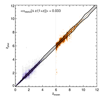
Figure 5 shows the input ‘known’ redshift against the best measured output redshift for all mock sources from $0<z<12$ . The full simulation contains $\sim$ 3.3M sources, 13K of which ( $\approx 0.4$ %) are at $6<z<12$ . Given the sheer number of sources in the catalog, we split the simulation into two regimes: at $z<6$ we only sample a random 1% subset of all sources for photometric redshift fitting (for computational ease); in other words, we fit photometric redshifts to $\sim$ 33K sources from $0<z<6$ . At $z>6$ we fit all galaxies so that we adequately sample the full range of true EoR source properties. Thus, in Figure 5, there appears to be a dearth of sources at $4\lower 2.15277pt\hbox{$\;\buildrel<\over{\sim}\;$}z<6$ due to this differential sampling of parameter space, but the apparent differential is simply visual (e.g., there are 1K sources modeled in the $4<z<6$ bin). To understand the improvement in the photometric redshifts provided by COSMOS-Web data, we compare our inferred mock photometric redshift quality to those from the COSMOS2020 catalog. Specifically, Weaver et al. (2022a) find that sources with $i$ -band magnitude between $25<i<27$ have 5% photometric redshift precision. Over the same $i$ -band magnitude range, we infer that these JWST data will improve that statistic to 2.5%. Both precisions are measured using the normalized median absolute deviation ( $\sigma_{\rm NMAD}$ ) of $\Delta z/(1+z)$ , a quantity analogous to the standard deviation of a Gaussian but less sensitive to outliers.

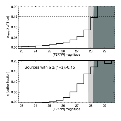
While this direct comparison is useful, we also calculate $\sigma_{\rm NMAD}$ for intrinsically fainter sources selected at longer wavelengths. We find that the median precision for sources with F277W magnitudes ranging 25–26.5 to be 2.3% across all epochs, and those with F277W magnitudes ranging 26.5–27.5 to be 4.2%. The right panel of Figure 5 shows how the photometric redshift precision is expected to degrade for sources as a function of F277W magnitude. Similarly, we investigate the outlier fraction, $\eta$ , as a function of magnitude, where outliers are defined as sources with $\Delta z/(1+z)>0.15$ . Outliers are below 10% for sources brighter than F277W $<27$ , increasing steeply to 20% near the 5 $\sigma$ detection limit at $\sim$ 28.2. Note that we analyze both the photometric redshift precision and outlier fraction as a function of redshift as well as magnitude; overall, both quantities are somewhat constant with redshift, with slight spikes in both from $6<z<7$ and $9<z<11$ , which is expected given the lack of complete filter coverage across expected break wavelengths at those redshifts. We analyze the efficacy of photometric selection for EoR galaxies further in § 4.1.3.

2.6 Expected Cosmic Variance

The areal coverage of COSMOS-Web represents a real strength of the program in the reionization era. With claims of potential massive galaxies in the distant universe from smaller surveys that, if confirmed, may challenge our models of galaxy formation, representative samples of the distant galaxy population would help establish the true luminosity function shape and evolution at early times.

Following Robertson (2010) (see also Trenti & Stiavelli, 2008), we estimate the $z\sim 9$ cosmic variance of the COSMOS-Web survey. We assume the survey area $A=0.54\deg^{2}$ , a depth of 27.6 magnitudes, and the $z\sim 9$ luminosity function parameters from Bouwens et al. (2021). We perform abundance matching between galaxies and the halo mass function, assigning the clustering strengths of halos to their hosted galaxies from the Tinker et al. (2010) peak background split model for the halo bias. We find that the cosmic sample variance uncertainty of COSMOS-Web at $z\sim 9$ is $\sigma_{v}\approx 16\%$ , and Poisson uncertainty is $\sigma_{p}\approx 8\%$ , which sum in quadrature to a total expected uncertainty of $\sigma_{tot}\approx 18\%$ (giving a total variance $\sigma_{v}^{2}=0.03$ ).

How does the cosmic variance of COSMOS-Web compare with the collection of smaller, deeper fields soon available with JWST coverage? Repeating our calculation for a single 100 arcmin² field to 29^th magnitude, we find such surveys have a $z\sim 9$ cosmic sample variance uncertainty of $\sigma_{v}\approx 34\%$ . Five 100 arcmin² fields probing independent sight lines have a combined cosmic sample uncertainty of $\sigma_{v}\approx 14\%$ , a Poisson uncertainty of $\sigma_{p}\approx 11\%$ and a total expected variance uncertainty of $\sigma_{tot}\approx 18\%$ . Thus COSMOS-Web has comparable statistical power to the combined power of other JWST Cycle 1 programs conducted over a smaller area to greater depth. As discussed in Robertson (2010), by combining these wide area and pencil beam surveys the degeneracies in the constraints on luminosity function parameters, like $M_{\star}$ , $\Phi_{\star}$ , or the faint-end slope $\alpha$ , can be broken or significantly ameliorated.

2.7 Scheduling of the Observations and First Epoch of Data

COSMOS-Web was awarded a total of 208 hours, but due to changes in overhead and the dithering pattern described above, COSMOS-Web will take a total of 255 hours to execute. We requested relatively low zodiacal background observations ( $<$ 10-20^th percentile) and to tile the mosaic at a nearly uniform position angle on the sky to avoid gaps within the mosaic. COSMOS-Web is observable in windows in April (PA $\approx$ 105) and December/January (PA $\approx$ 290) of each year. In order to maximize the amount of overlap between the prime (NIRCam) and parallel (MIRI) observations, we will observe roughly half of the mosaic in each window.

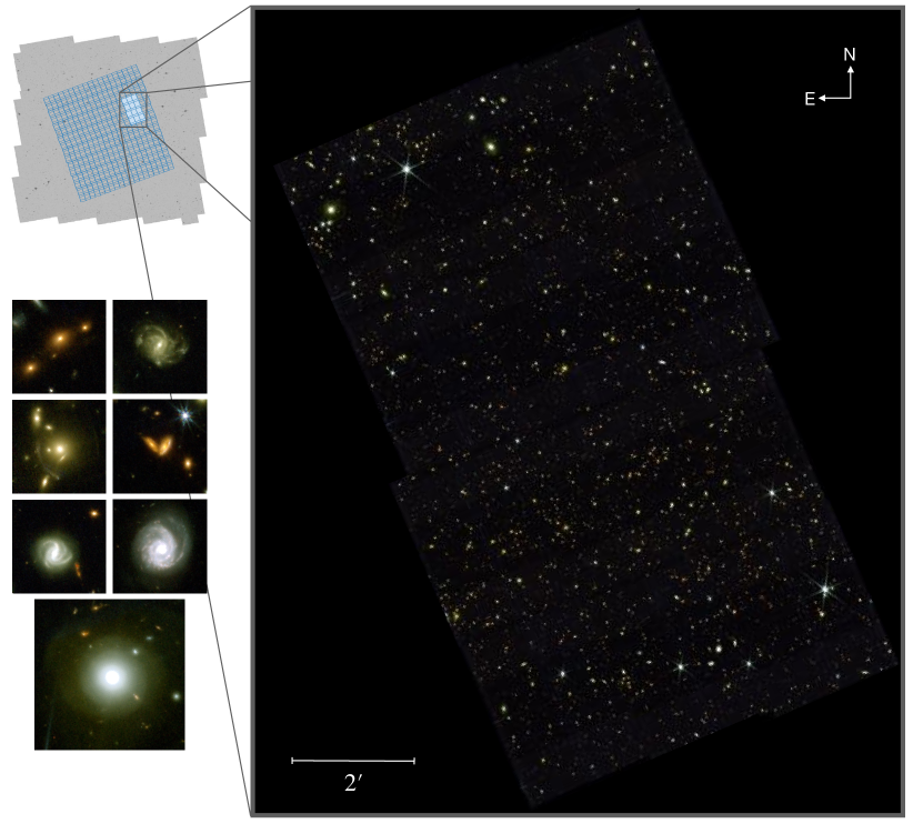
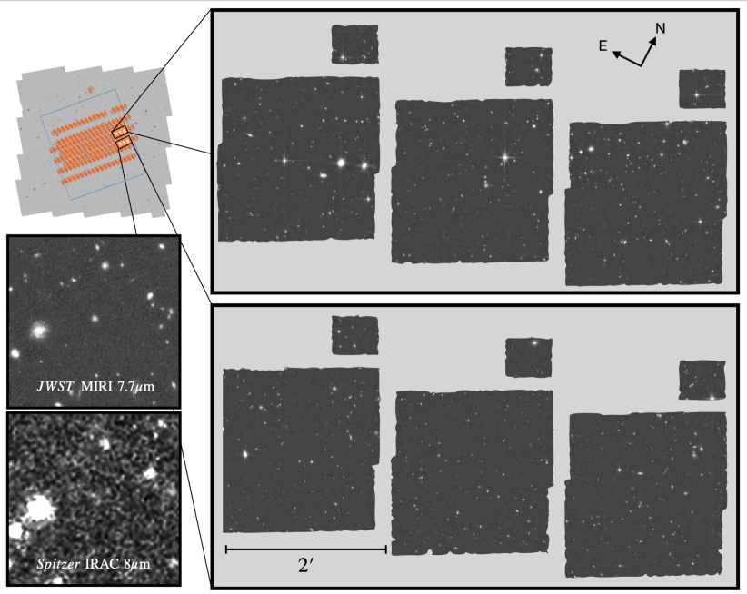
The first epoch of observations consists of six visits covering $\sim$ 77 arcmin² with NIRCam and was observed on 5-6 January 2023. Figure 6 shows the NIRCam mosaic of this region of the field, which is 4% of the final dataset. Figure 7 shows the six MIRI tiles from this epoch. As of this writing, 77 pointings are scheduled for April/May 2023 (roughly half the field) and the remaining 69 pointings in December 2023/January 2024. The COSMOS-Web team will release mosaics registered to Gaia astrometry after each subsequent epoch of observations is taken through the Mikulski Archive for Space Telescopes (MAST) and the NASA/IPAC Infrared Science Archive (IRSA); we will also make these mosaics accessible through the IRSA COSMOS cutout service⁴⁴4https://irsa.ipac.caltech.edu/data/COSMOS/index_cutouts.html.

Table 3: JWST Cycle 1 NIRCam Surveys

Survey	Fields	Area	SW Filters	LW Filters	Depth
Name	Observed	arcmin²
NGDEEP	HUDF-Par2	10	F115W, F150W, F200W	F277W, F356W, F444W	30.6–30.9
UDF-Medium	HUDF	10	F182M, F210M	F430M, F460M, F480M	28.0–29.8
JADES-Deep	HUDF	46	F090W, F115W, F150W, F200W	F277W, F335M, F356W, F410M, F444W	30.3–30.7
JADES-Medium	GOODS-N, GOODS-S	190	F070W $\dagger$ , F090W, F115W, F150W, F200W	F277W, F356W, F410M, F444W	29.1–29.8
CEERS	EGS	100	F115W, F150W, F200W	F277W, F356W, F410M, F444W	28.4–29.2
PRIMER	COSMOS, UDS	378	F090W, F115W, F150W, F200W	F277W, F356W, F410M, F444W	27.6–29.5
COSMOS-Web	COSMOS	1929	F115W, F150W	F277W, F444W	26.9–28.3

Note. — Depths quoted are 5 $\sigma$ point source depths. NIRCam depths quoted have been drawn from the original proposals and pre-flight exposure time calculator estimates within 0 $\farcs$ 15 radius circular apertures. We have not adjusted for the in-flight calibration (Boyer et al., 2022) of the instruments; however, any differences with these figures is anticipated to be of order smaller than a 10% effect, smaller than the typical deviation across a mosaic stitched together with non-uniform depth, or from variation in depth filter-to-filter. Program IDs for these surveys are: NGDEEP (GO # 2079), UDF-Medium (GO # 1963), JADES-Deep (GTO # 1180, 1210, 1287), JADES-Medium (GTO # 1180, 1181, 1286), CEERS (ERS # 1345), PRIMER (GO # 1837), and COSMOS-Web (GO # 1727). $\dagger$ F070W in JADES-Medium imaging is only planned for parallel coverage areas currently lacking HST.

Table 4: JWST Cycle 1 MIRI Surveys

Survey	Fields	Area	Filters	Depth
Name	Observed	arcmin²
MIRI-HUDF-Deep^†	HUDF	2.5	F560W	28.3–28.5
CEERS	EGS	13	F770W, F1000W, F1280W, F1500W, F1800W, F2100W	21.6–26.3
JADES-Medium	HUDF^∗	10	F770W	27.1
	GOODS-N, HUDF	17.5	F770W, F1280W	24.7–25.4
MIRI-HUDF-Medium	HUDF	30	F560W, F770W, F1000W, F1280W	23.3–24.8
			F1500W, F1800W, F2100W, F2550W	19.8–23.2
PRIMER	COSMOS, UDS	137	F770W, F1800W	22.1–25.4
COSMOS-Web	COSMOS	697	F770W	24.0–25.1^‡

Note. — Depths quoted are 5 $\sigma$ point source depths within 0 $\farcs$ 3 radius circular apertures from the exposure time calculator. Program IDs for these surveys are: CEERS (ERS # 1345), MIRI-HUDF-Medium (GO # 1207), MIRI-HUDF-DEEP (GO # 1283), JADES-Medium (GTO # 1180 and 1181), PRIMER (GO # 1837), and COSMOS-Web (GO # 1727). $\dagger$ Note that the MIRI-HUDF-Deep Program (GO # 1283) is nested within the MIRI-HUDF-Medium (GO # 1207) program, but both are spatially offset from the JADES-Medium HUDF coverage. ^∗ Note that the deeper part of JADES-Medium HUDF F770W coverage is nested within the shallower JADES-Medium coverage. ^‡ Note that the depth quoted here for COSMOS-Web differs from the reported measured depth as given in Table 2; similarly, PRIMER and CEERS measured depths differ from ETC estimates, with measured 7.7 $\mu$ m depths of those programs shown in Figure 8. What is quoted in this table is from the exposure time calculator. We expect the actual depth of all MIRI programs to differ from ETC estimates in a similar manner.

3 Context of COSMOS-Web Among Other JWST Deep Fields

Several extragalactic deep field surveys will be conducted in the first year of JWST observations that span a range of areas, depths, and filter coverage; their approximate depths and areas are described in Table 3 for NIRCam programs and Table 4 for MIRI programs. Note that the NIRCam depths of other programs quote the pre-flight exposure time calculator (ETC) estimates and do not necessarily reflect the actual final measured depths of the data. For MIRI, we include the measured depths from COSMOS-Web, CEERS, and PRIMER observations along with the updated ETC estimates. The MIRI depth in COSMOS-Web is measured to be significantly deeper (by $\sim$ 1 magnitude) compared to the ETC estimates. We refer the reader to the recent review by Robertson (2022), their § 8.2, as well as their Figure 6, for a summary of many of the large extragalactic programs, and in particular their NIRCam coverage. These programs include the Guaranteed Time Observation (GTO) programs allocated to the instrument teams, the Director’s Discretionary Early Release Science Programs (ERS), as well as the General Observer (GO) Cycle 1 programs.

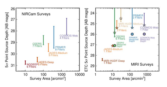
Figure 8 shows the relative depth and survey area of the major broad-band legacy extragalactic programs in Cycle 1, both for NIRCam imaging and MIRI imaging programs. To briefly summarize the relative scope of the NIRCam programs, the deepest surveys are NGDEEP⁵⁵5NGDEEP was originally named WDEEP at the time of the proposal. (GO #2079) and the JADES GTO Survey (in particular GTO #1180, 1210, & 1287). These collectively cover about $\sim$ 0.05 deg² to depths exceeding $\sim$ 29.5 mag in several broad-band filters. The medium depth programs JADES-Medium (including parts of GTO #1180, 1181, and 1286), CEERS (ERS #1345), and PRIMER (GO #1837) together cover a total of $\sim$ 0.18 deg² to a depth $\sim$ 28–29 mag. Note that the UDF Medium Band Survey (GO # 1963) achieves similar depths $\sim$ 28–29.8 mag in NIRCam medium bands over 10 arcmin² in the HUDF (an area also covered by JADES-Deep in the broad-bands). COSMOS-Web (GO #1727) is the shallowest but largest program to be observed, covering a total 0.54 deg² with NIRCam to a depth of $\sim$ 27.5–28.2 mag across the field.

Planned MIRI programs vary in depth more substantially, as the shorter wavelength filters achieve much deeper observations per fixed exposure time. The MIRI GTO programs adopt two very different approaches: one (GO # 1283) goes quite deep in a single MIRI pointing in one filter, F560W. The other (GO # 1207) covers 30 arcmin² and uses all 8 broad-band MIRI filters and thus is significantly more shallow. MIRI imaging is obtained in parallel to much of the JADES program (from programs GTO #1180 and 1181) where a hybrid approach was adopted, going deep in one filter, F770W, over 10 arcmin², and shallower in two filters, F770W and F1280W, over 15 arcmin². CEERS similarly spans a broad range in depths over 13 arcmin² using 6 filters, and PRIMER covers much larger areas over $\sim$ 140 arcmin² in two filters. Similar to its NIRCam coverage, COSMOS-Web covers the largest area with MIRI, but with variable depth (based on the number of exposures) in F770W. We have shown the F770W depths of the MIRI surveys using a star in Figure 8 for more direct comparisons to the COSMOS-Web depths.

The total area covered by COSMOS-Web in NIRCam is roughly 2.7 $\times$ larger than the other planned JWST extragalactic deep fields combined. For MIRI, COSMOS-Web’s coverage is 3.5 $\times$ larger than all other deep field programs combined. The extraordinary range of areas and depths of deep field surveys observed in JWST’s first year will be complementary, and enable a wide range of scientific studies, spanning the most distant and faintest galaxies ever detected to the most comprehensive environmental studies of the distant universe.

4 Scientific Goals

The scientific breadth of COSMOS-Web has the potential to be extraordinary, with an estimated $\sim$ 10⁶ sources to be detected from $z\sim 0.1$ to cosmic dawn. Nevertheless, the survey as proposed was motivated by three key science areas that ultimately drive the design of the survey. The three primary goals of the program are to:

1.

forge the detection of thousands of galaxies in the Epoch of Reionization ( $6\lower 2.15277pt\hbox{$\;\buildrel<\over{\sim}\;$}z\lower 2.15277pt\hbox{$\;\buildrel<\over{\sim}\;$}11$ ) and use their spatial distribution to map large scale structure during the Universe’s first billion years,
2.

identify hundreds of the rarest quiescent galaxies in the first two billion years ( $z>4$ ) to place stringent constraints on the formation of the Universe’s most massive galaxies (with $M_{\star}>10^{10}$ M_⊙), and
3.

directly measure the evolution of the stellar mass to halo mass relation (SMHR) out to $z\sim 2.5$ and its variance with galaxies’ star formation histories and morphologies.

Below we detail the motivation and requirements of each science goal.

4.1 Mapping the Heart of Reionization

The first galaxies formed $<\,1$ Gyr after the Big Bang are thought to drive the last major phase change of the Universe from a neutral to ionized intergalactic medium (IGM). This reionization process (Robertson et al., 2015) most likely finished around $z\sim 6$ (Zheng et al., 2011; Kakiichi et al., 2016; Castellano et al., 2016; Ouchi et al., 2020) and was halfway completed by $z\sim 7-8$ , according to measures of the rest-frame UV galaxy luminosity function (UVLF; Finkelstein, 2016). This is in broad agreement with the Planck constraint of the instantaneous reionization redshift $z_{\rm reion}=7.7\pm 0.8$ (Planck Collaboration et al., 2020). However, neither the start and duration of reionization, nor the sources responsible — either intrinsically luminous galaxies or more intermediate mass galaxies (Naidu et al., 2020; Hutter et al., 2021) — are well-constrained due to the relative shortage of both bright and faint $z\sim 7-11$ galaxies known in the pre-JWST era. Additional complexity is introduced by potentially significant evolution in the nature of EoR galaxies themselves: their intrinsic star formation rates (SFR), ionizing power ( $\xi_{\rm ion}$ ), ionizing radiation escape fraction ( $f_{\rm esc}$ ), number density, physical distribution, and clustering.

Constraining the physics of reionization requires identifying and characterizing the galaxies that are embedded deep within the predominantly neutral Universe at $z\lower 2.15277pt\hbox{$\;\buildrel>\over{\sim}\;$}$ 8, though direct detection of EoR galaxies has been challenging to-date. Pioneering work with Hubble led to the discovery of $\sim$ 80 candidate Lyman Break Galaxies (LBGs) at $z>8$ (see review by Finkelstein, 2016). Despite the perceived rapid drop in the UVLF during this epoch (Oesch et al., 2014), there have been a few successful pre-JWST detections of surprisingly bright candidate LBGs out to $z\sim 11$ (the most spectacular of which is GNz11 at $z=10.6$ , Oesch et al. 2016; Jiang et al. 2021; Bunker et al. 2023). Although these $z>8$ galaxies are thought to reside in a predominantly neutral Universe, somehow a number of them show Ly $\alpha$ in emission (e.g., Oesch et al., 2015; Zitrin et al., 2015; Hoag et al., 2018; Hashimoto et al., 2018; Pentericci et al., 2018). This is surprising given that those Ly $\alpha$ photons should have been resonantly scattered by the mostly neutral IGM (Dijkstra, 2014; Stark, 2016; Garel et al., 2021). Do these Ly $\alpha$ emitters at $z>8$ live in special ‘ionized’ bubbles? If they are representative of the general population, are we missing some fundamental aspect of the first stage of reionization? These questions can only be answered with a large sample of bright $z=7-11$ sources across a range of large scale environments, only possible with a near-IR contiguous wide-area survey (Kauffmann et al., 2020).

The first candidate discoveries of unusually bright galaxy candidates identified in early JWST observations (e.g., Naidu et al., 2022a; Finkelstein et al., 2022a, b; Donnan et al., 2022; Harikane et al., 2022; Atek et al., 2022) suggest that these sources may not be as rare as our pre-JWST models of $z>7$ galaxy formation would indicate (e.g., Mason et al., 2015; Yung et al., 2019, 2020; Behroozi et al., 2020; Wilkins et al., 2017, 2022). While we note that these early discoveries are still candidates that require spectroscopic confirmation (as of this writing only a few $z>9$ systems have been spectroscopically-confirmed, Roberts-Borsani et al., 2022; Williams et al., 2022; Robertson et al., 2022a; Curtis-Lake et al., 2022), the perceived wealth of bright candidates may be particularly relevant to understanding the distribution of galaxies within large scale structure at early times. These bright candidates theoretically occupy the rarest and most massive dark matter halos, which are thought to be more highly clustered, and as such, small area surveys (as has been carried out to-date with JWST) would poorly constrain their volume densities and the environments in which they live.

The breadth of galaxies’ environments at early times is closely related to how reionization propagated. It is thought that reionization was predominantly a patchy process, producing ionized bubbles in the surrounding IGM growing from 5 – 20 Mpc at $z>8$ to 30 – 100 Mpc at $z\sim 7$ (Furlanetto et al., 2017; D’Aloisio et al., 2018). This corresponds to angular scales of 10 – 40 arcmin across, much larger than all contiguous NIR deep fields from Hubble or other planned deep field areas from JWST (see Table 3. Furthermore, large variance in the IGM’s opacity from $5<z<7$ quasar sightlines (Becker et al., 2015) suggests that the patchiness exceeds theoretical expectation from the density field alone by factors of a few, exacerbating uncertainties in reionization constraints from cosmic variance in existing surveys. Follow-up studies around both transparent and opaque quasar sightlines indicate a wide variety of large scale environments (Becker et al., 2018; Davis et al., 2018).

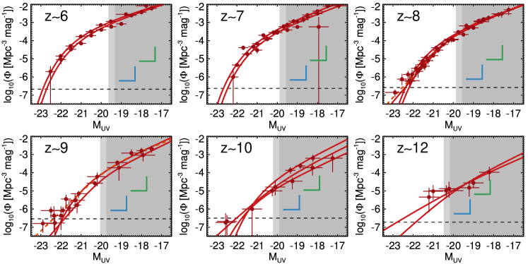
COSMOS-Web will grow the census of EoR ( $z>6$ ) galaxies beyond what is known from Hubble surveys by a factor of $\sim$ 5 and quantify the evolution of the UVLF, stellar mass function (SMF), and star formation histories of galaxies across the Universe’s first billion years. By observing a large contiguous area, COSMOS-Web will detect a factor of $\sim$ 6-7 times more sources at or above the knee of the luminosity function, $L_{\star}$ , than expected from all other JWST deep field efforts combined. Figure 9 shows the aggregate UVLF measurements from the literature to-date from $6<z<13$ , combining Hubble samples with the most recent results from JWST. Table 5 gives statistics on the predicted number of EoR galaxies to be found in COSMOS-Web, calculated directly from the compiled UV luminosity functions, relative to other Cycle 1 medium and deep programs.

Massive galaxies above $L_{\star}$ are most likely to trace the highest-density peaks from which the reionization process was likely to begin. In particular, the 0.54 deg² survey area of COSMOS-Web is sufficiently large to capture reionization on scales larger than its expected patchiness, minimizing the effect of cosmic variance. As a contiguous survey, COSMOS-Web will sample the full range of environments at this epoch, provided large scale structure is clustered on scales within an order of magnitude of their predicted scales (Gnedin & Kaurov, 2014). This contrasts with, for example, the innovative Hubble and JWST pure-parallel surveys (e.g., BoRG, Schmidt et al. 2014; Calvi et al. 2016 and PANORAMIC, GO #2514) that, by design, will sample a wide variety of environments but cannot directly map the large scale environments of their discoveries.

Table 5: Number of Sources Expected between

6<z<13

in Cycle 1 Programs

Survey	$z\sim 6$	$z\sim 7$	$z\sim 8$	$z\sim 9$	$z\sim 10$	$z\sim 12$
	( $\Delta z=1$ )	( $\Delta z=1$ )	( $\Delta z=1$ )	( $\Delta z=1$ )	( $\Delta z=1.5^{*}$ )	( $\Delta z=2$ )
COSMOS-Web	2900–4000	1000–1500	500–680	150–160	30–70	12–25
All Medium Cy 1 Programs^†	3800–5000	1600–2400	1000–1300	230–450	70–260	37–44
All Deep Cy 1 Programs^‡	900–1100	450–640	310–350	90–150	20–100	13–15
Medium Cy 1 at COSMOS-Web Depth	1300–1700	460–680	230–300	30–80	14–36	5–11
Deep Cy 1 at COSMOS-Web Depth	110–150	40–60	19–26	3–7	1–3	0–1
COSMOS-Web Depth in $M_{\rm UV}$	–19.3	–19.6	–19.6	–19.7	–19.9	–20.2

Note. — Here we refer to all ‘medium’ depth Cycle 1 programs ( $\dagger$ ) as surveys reaching $\sim$ 28.5–29.5 mags in broad-band filters from Table 3, including JADES-Medium, CEERS and PRIMER. The ‘deep’ Cycle 1 programs ( ${\ddagger}$ ) refer to JADES-deep and NGDEEP together, which will reach depths exceeding 29.5 mags. ^∗ Note that the $z\sim 10$ bin spans $9.5<z<11$ .

4.1.1 Impact beyond $z>8$

Beyond the halfway point of reionization, COSMOS-Web is likely to detect hundreds of intrinsically bright galaxies at $8<z<11$ embedded deep in the predominantly neutral IGM. This will increase the number of known $z>8$ galaxies from the pre-JWST era by a factor of 10 above a luminosity of $L_{\star}$ . Through such a transformative sample of luminous $z>8$ candidates, these discoveries will allow the first constraints on the bright-end of the UVLF and SMF at $z\lower 2.15277pt\hbox{$\;\buildrel>\over{\sim}\;$}8$ with minimal uncertainty from cosmic variance, minimized to $\;\buildrel<\over{\sim}\;$ 10% on scales of 0.5 deg² at our detection threshold of $\sim$ 27.5 magnitudes (Behroozi et al., 2019). Table 5 shows the expected total number of sources COSMOS-Web will find, totaling to $\sim$ 600–900 above $z>8$ and 12–25 from $11<z<13$ .

Our NIRCam filter combination is specifically optimized for $8<z<11$ galaxy selection above the F115W detection limit of $\sim$ 27.4 mag as shown in Figure 3. Such systems are expected to see a significant drop in the F115W filter. If we account for a possible deviation from a Schechter UVLF as measured by wide/shallow ground-based UVLF estimates at $z>8$ (shown as double power laws in Figure 9), our detections will likely exceed 1000 sources above $z>8$ , sufficient to map their spatial distribution and trace large scale structure at such early times. Even with our fiducial expectations in 0.54 deg² coverage, we expect to see a factor of $\sim$ 7 improvement in the number of $z>8$ candidate galaxies above $L_{\star}$ over all previous Hubble work and a factor 2 $\times$ larger samples at those luminosities than all other planned Cycle 1 programs combined.

4.1.2 Inferring the bright-end shape of the UVLF and SMF

While CANDELS found only $\sim$ 2 – 10 galaxies at $z>6$ with $M_{\star}>10^{10.5}$ M_⊙, and none above 10¹¹ M_⊙ (Grazian et al., 2015; Song et al., 2016), the wider Ultra-VISTA survey (Bowler et al., 2014, 2020) found a larger number of massive galaxies than expected based on an extrapolation of a Schechter function fit to the CANDELS-measured SMF. The recent candidate discovery of intrinsically bright $z>10$ galaxies in small-area early release JWST observations (e.g., Naidu et al., 2022a; Castellano et al., 2022; Finkelstein et al., 2022a, b; Donnan et al., 2022; Atek et al., 2022) also hint at a possible overabundance of massive galaxies compared to a Schechter function expectation. This excess of bright sources could indicate that the most massive galaxies are highly clustered and/or that the SMF at $z>6$ departs from Schechter (Bowler et al., 2017; Davidzon et al., 2017). COSMOS-Web will greatly improve the dynamic range of luminosities (and thus masses) probed beyond all other NIR surveys, detecting $\sim$ 280–500 bright $M_{\rm UV}<-21$ galaxies at $z\sim 6-8$ and $\sim$ 30–80 at $8<z<13$ , corresponding to stellar masses $\lower 2.15277pt\hbox{$\;\buildrel>\over{\sim}\;$}4\times$ 10⁹ M_⊙. We calculate these estimates using the literature parameterized luminosity functions shown in Figure 9 integrated down to $M_{\rm UV}=-21$ , significantly above our detection threshold as detailed in Table 5. Given these statistics, a Schechter UVLF will be distinguishable from a double power-law in this dataset at a minimum of $\sim$ 4 $\sigma$ out to $z=9$ ; this estimate is based on the Poisson uncertainties in the expected number of sources to-be-discovered in COSMOS-Web given a Schechter function and a conservative estimate on the bright-end slope of the UVLF in the case of a double power-law (using $\beta=-4$ ). Such a deviation could be indicative of a primordial galaxy formation stage with different star formation timescales (Finkelstein et al., 2015; Yung et al., 2019), a lack of dust, or before the onset of feedback from Active Galactic Nuclei (AGN).

4.1.3 Selection of EoR Sources

As discussed in § 2.5, we generate a mock lightcone of the COSMOS-Web field containing an idealized sample of $0<z<12$ galaxies, and here we use that simulated photometric catalog to diagnose contamination and precision of our EoR photometric redshifts, applying tools we will use for the real dataset.

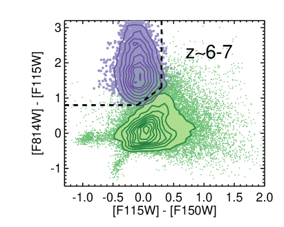
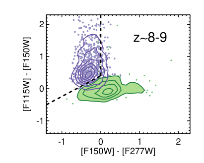
Figure 10 highlights the distribution of mock galaxies in color-color space for $z\sim 6-7$ and $z\sim 8-9$ galaxies against potential contaminating populations. The primary contaminants in both redshift regimes are $1<z<4$ faint galaxies ( $\sim$ 27^th mag). The F814W and F115W filters are effective drop out filters for the two redshift regimes, though small gaps in wavelength coverage between filters imply that photometric redshift precision in COSMOS-Web will be somewhat less accurate than in fields with more complete filter coverage. We find that contamination rates are most significant (up to $\sim$ 20%) within 0.5 magnitudes of our 5 $\sigma$ point source detection limit, where the constraint on drop filters is slightly weaker. We also anticipate relatively elevated contamination ( $\sim$ 20%) in the redshift range $5.5<z<6.5$ due to both the gap between F814W and F115W as well as the relative depth difference between the filters (where F814W is shallower but also serves as the drop out filter). For $6.5<z<9.5$ , we anticipate contamination rates below $\sim$ 10% with a photometric redshift precision of $\Delta z/(1+z)\approx 0.02-0.04$ . Above $z\sim 9.5$ , the precision of photometric redshifts is degraded substantially by the lack of coverage at 2 $\mu$ m (see Figure 3); while some candidate $z>12$ sources may be identified, they would require spectroscopic follow-up to confirm their redshifts, as NIRCam photometry would not constrain them very precisely. We will present further analysis of photometric redshift precision, as well as EoR sample contamination and completeness, in a forthcoming COSMOS-Web paper on the rest-frame UV luminosity function (Franco et al., in preparation).

An important consideration for the selection of EoR galaxy candidates will also be contamination of samples with lower redshift strong nebular emission line sources. For example, an underlying dust obscured (and reddened) rest-frame optical continuum superimposed with strong emission lines can masquerade as a bluer rest-frame UV continuum in JWST’s broadband filters, as shown by Zavala et al. (2022) and Naidu et al. (2022b). In that case one might expect dust continuum emission at millimeter wavelengths, representing reprocessed emission from hot stars. However, Fujimoto et al. (2022a) demonstrates that even a lack of dust continuum emission cannot rule out possible contamination from type-II quasars or AGN (in this case, the area covered with MIRI in F770W could lead to the detection of AGN that satisfy LBG selection criteria; Fujimoto et al., 2022b). While these possible foreground contaminants have come to light with the identification of ultra high-redshift sources ( $z>12$ ), it is nevertheless an important consideration in the identification of all EoR candidates, given the relatively sparse broad-band sampling available to select such sources. Follow-up spectroscopy of many EoR candidates in the next year will elucidate the level of contamination present in such samples and play a crucial role in informing statistics about large samples selected in COSMOS-Web.

4.1.4 The first maps of LSS during the EoR

The full 0.54 deg² COSMOS-Web survey will allow the direct construction of large scale structure density maps of galaxies spanning $z\sim 6-10$ . Such snapshots of the density field will provide a direct test as to whether or not the brightest, most massive galaxies are indeed highly clustered, as suggested by cosmological simulations (e.g., McQuinn et al., 2007; Behroozi et al., 2013; Chiang et al., 2017). Though some massive galaxies have been identified at this epoch from Ultra-VISTA data (Bowler et al., 2020; Endsley et al., 2022b; Kauffmann et al., 2022), it remains to be seen whether or not they sit in overdense environments. Existing Hubble and other planned JWST surveys are insufficient to answer this question due to their limited areas, however, COSMOS-Web will have both the depth and area to enable this measurement.

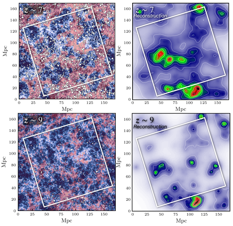
Figure 11 illustrates our approach by using a mock catalog from a cosmological simulation (GADGET2; Springel, 2005) at $z\sim 7$ with width $\Delta z\approx 0.5$ (and $z\sim 9$ with width $\Delta z\approx 0.7$ ) to reconstruct the underlying density map from simulations using the weighted adaptive kernel smoothing technique (Darvish et al., 2015) on 5 Mpc scales. We have used this simulation to directly test our ability to reconstruct the density field of galaxies from detectable sources. We infer that we will be able to reconstruct $\sim$ 12 independent mappings of the full density field between $6<z<10$ based on our simulated photometric precision ( $\Delta z/(1+z)\sim 0.02-0.04$ ) and low contamination rates using a combination of color cuts and photometric redshift fitting (see § 4.1.3). The smoothing scale of 5 Mpc is an ideal scale to achieve a S/N in the overdensity measurement of $>5\,\sigma$ per beam and S/N $>20\,\sigma$ per overdense structure (with $>25$ galaxies per beam in the highest density regions). COSMOS-Web will provide the first direct measurement of the physical scale and strength of overdensities at these epochs for direct comparison to the hypothesized scale of reionization-era bubbles that theoretically emanate from them.

4.1.5 Masses of EoR Galaxies

COSMOS-Web will enable crucial stellar mass constraints for the most massive EoR galaxies via the detection of rest-frame optical light (e.g., Faisst et al. 2016). In particular, with the MIRI F770W observations covering 0.19 deg², we expect to detect 90-130 galaxies at $6<z<8$ and 2–3 galaxies at $8<z<10$ based on estimates from the UVLF. This would double the expected number of EoR galaxies with rest-frame optical detections from the other Cycle 1 JWST programs. At these redshift regimes this corresponds to rest-frame 1 $\mu$ m and 7700 Å light, respectively. This will place unique constraints on the physical characteristics of extremely rare M ${}_{\star}\lower 2.15277pt\hbox{$\;\buildrel>\over{\sim}\;$}10^{10}$ M_⊙ galaxies in the Universe’s first few hundred Myr for the subset of EoR sources that we expect to detect with MIRI, as no galaxies with these high masses are expected to be found in the other Cycle 1 JWST surveys that cover smaller areas (cf. the sources identified by Labbe et al., 2022, with extreme stellar masses established at $z\sim 7-9$ ; though those sources’ stellar masses may yet be highly uncertain, e.g., Endsley et al. 2022a). The detection of $\sim$ 100 galaxies in this mass regime will provide important clues to the star formation histories of the Universe’s most massive halos in the first Gyr after the Big Bang, which are currently unconstrained.

4.1.6 Follow-up of EoR Sources

Beyond the direct EoR discoveries that COSMOS-Web will make through its JWST imaging, follow-up observations will further enhance the impact of this program and shed light on key unknowns. These include (1) rest-frame UV diagnostics with JWST NIRSpec that will constrain ionizing photon production in $z\lower 2.15277pt\hbox{$\;\buildrel>\over{\sim}\;$}6$ sources (i.e., constraints on $f_{\rm esc}$ and $\xi_{\rm ion}$ , e.g., Chisholm et al., 2020), (2) deep rest-frame UV observations of Ly $\alpha$ to infer local variations in the IGM neutral fraction with Keck, Subaru, VLT (which can typically reach line sensitivities of $\sim$ 10^-18 erg s^-1 cm^-2), and future 30 m-class telescopes (the extremely large telescopes, ELTs, that will push fainter), and (3) obscured star-formation and cold ISM content of dust and metals from ALMA detections of the FIR continuum and the FIR fine-structure atomic cooling lines (Laporte et al., 2017; Hashimoto et al., 2018; Bakx et al., 2022; Fujimoto et al., 2022a), which will inform stellar population synthesis models of galaxies’ first light, metals, and dust. COSMOS-Web, as a wide and shallow survey, will be particularly useful for the detection of bright, rare candidates that are well optimized for ground-based follow-up. These future observations will be crucial for detailed characterization of EoR overdensities, unlocking direct comparisons between mapped reionization bubbles (measured via Ly $\alpha$ follow-up) and JWST-measured density maps, as shown from a simulation in Figure 11.

4.2 The Buildup of the Massive Galaxy Population

The wide-area coverage of COSMOS-Web, in particular the combination of the NIRCam LW (2.8 $\mu$ m and 4.4 $\mu$ m) and MIRI (7.7 $\mu$ m) observations with the already existing wealth of optical to NIR data in COSMOS, will allow us to take the first census of massive galaxies from the end of the EoR to the peak of galaxy assembly. Within the footprint of COSMOS-Web, we expect firm identification of half a million galaxies at all redshifts, $\sim$ 32,000 of which will be detected in MIRI F770W imaging, allowing us to constrain stellar masses, sizes, morphologies, star formation rates, and AGN activity for galaxies across a wide swath of cosmic time.

4.2.1 The First Quiescent Galaxies

The growing census of massive quiescent galaxies at early epochs ( $M_{\star}\lower 2.15277pt\hbox{$\;\buildrel>\over{\sim}\;$}10^{10}\,$ M_⊙ out to $z\sim 3-5$ , e.g., Straatman et al., 2014; Glazebrook et al., 2017; Schreiber et al., 2018; Merlin et al., 2019; Tanaka et al., 2019; Girelli et al., 2019; Valentino et al., 2020; Forrest et al., 2020; Carnall et al., 2022, 2023; Rodighiero et al., 2022) has presented a strong challenge to theoretical models of early massive galaxy formation (e.g., Feldmann et al., 2016; Steinhardt et al., 2016; Cecchi et al., 2019, see Figure 12). In order to build up their significant stellar masses and quench their star formation so early in the Universe’s history, these galaxies must have formed their stars at exceptionally high rates ( $\gg$ 100 M_⊙ yr^-1, comparable to luminous infrared galaxies; Sanders & Mirabel 1996, and dusty star-forming galaxies, DSFGs; Casey, Narayanan, & Cooray 2014) at very early times and then abruptly shut down the production of stars well within the Universe’s first Gyr. The existence of these sources and their relative abundance provide important tests of the galaxy assembly process and the physical processes driving the quenching of star formation at this early epoch.

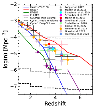
The quiescent galaxy mass function beyond $z\sim 4$ is currently unconstrained, partly because of the difficulty of detecting these rare galaxies in existing deep field observations (with volume densities $\lower 2.15277pt\hbox{$\;\buildrel<\over{\sim}\;$}10^{-5}$ Mpc^-3) and partly because such galaxies are particularly difficult to separate from DSFGs and post-starburst galaxies that can mimic the same red colors (see Figure 3). Detecting them requires deep rest-frame optical observations over wide areas of the sky. COSMOS-Web will provide the ideal dataset for identifying candidate quiescent galaxies and measuring (or placing constraints) on their number densities and relative abundances. Figure 12 highlights the expected number density of massive (M ${}_{\star}>10^{10}$ M_⊙) quiescent (specific SFR, SFR/M ${}_{\star}<10^{-11}$ yr^-1) galaxies from the cosmological hydrodynamical simulations IllustrisTNG100 (Pillepich, 2018), EAGLE (McAlpine et al., 2016), and FLARES (Lovell et al., 2022), as well as the DREaM semi-empirical model (Drakos et al., 2022) and predictions from the empirical model of Long et al. (2022), in comparison to some of the currently identified quiescent galaxy candidates in the literature (Muzzin et al. 2013; Straatman et al. 2014; Merlin et al. 2019; Schreiber et al. 2018; Girelli et al. 2019; Shahidi et al. 2020; Carnall et al. 2022; Weaver et al. 2022b; Gould et al. 2023; Valentino et al. 2023). Note that each study selects quiescent galaxies slightly differently, and the resulting samples span a range of stellar mass cuts, with the vast majority of candidates having M ${}_{\star}>10^{10}$ M_⊙. When multiple mass cuts are quoted by a given study, we show number densities above this mass limit for consistency.

The quiescent galaxy sample from IllustrisTNG100 was selected using the publicly available⁶⁶6https://www.tng-project.org/data/ star formation rate (Pillepich, 2018; Donnari et al., 2019) and stellar mass value that corresponds to the mass within twice the half-mass radius of each object (Rodriguez-Gomez et al., 2016). Note that there are no quiescent galaxies in the IllustrisTNG100 volume beyond $z>4$ using this definition. We similarly selected the quiescent galaxy sample from the public EAGLE galaxy database⁷⁷7https://icc.dur.ac.uk/Eagle/database.php (McAlpine et al., 2016) using the recommended aperture size of 30 physical kpc. These hydrodynamical simulations are calibrated to reproduce physical properties in the local Universe and predict the the SFR and M_⋆ values at high redshift. For FLARES, we use the number densities measured by Lovell et al. (2022). These simulations generally underpredict the observed number densities of quiescent galaxies in the literature (though the observations span a wide range of values). On the other hand, semi-analytic models like DREaM are calibrated to match scaling relations at all redshifts. The DREaM number densities in Figure 12 are based on the SMF of Williams et al. (2018) and are a close match to the high end of the observed number densities.

Even though true quiescent galaxies are expected to be rare at $z>4$ , with the large area of COSMOS-Web we will be able to identify massive quiescent galaxy candidates and place robust constraints on their abundances as a function of redshift if they are brighter than our detection limit with number densities $\geq$ 10^-7 Mpc^-3. This measurement will also be less impacted by the effects of cosmic variance than similar measurements from smaller area surveys (e.g., Carnall et al. 2022).

The combination of NIRCam and MIRI filters over 0.20 deg² (including the COSMOS-Web and PRIMER MIRI imaging that fall within the NIRCam footprint) will enable quiescent galaxies to be distinguishable from dusty star-forming interlopers via color-selection and SED analysis using the well-sampled rest-frame optical photometry. Additionally, the complementary (sub)millimeter observations over the COSMOS field (see Figure 4) will enable the direct identification of dusty galaxies at $z>4$ and therefore disentangle them from quiescent and EoR galaxy candidates (see Zavala et al. 2022; Naidu et al. 2022b; Fujimoto et al. 2022a for detailed discussion of the difficulty in separating these populations using NIRCam colors alone). Specifically, the existing SCUBA-2 and future TolTEC observations will cover COSMOS to a depth of SFR $\;\buildrel>\over{\sim}\;$ 50 M_⊙ yr^-1, while the ALMA MORA survey (Zavala et al., 2021; Casey et al., 2021; Manning et al., 2022) and its continuation (ex-MORA; Long et al., in preparation) will cover 0.2 deg² ( $\sim$ 1/3 of COSMOS-Web), in addition to the public ALMA archival pointings from A3COSMOS (totalying 0.12 deg² across all of COSMOS; Liu et al., 2019) and will directly detect DSFGs at $z>4$ in excess of SFR $\;\buildrel>\over{\sim}\;$ 100 M_⊙ yr^-1.

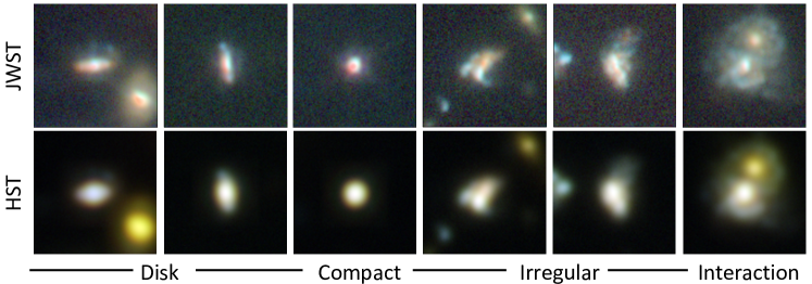
In addition to identifying the highest redshift quiescent galaxies, COSMOS-Web observations will allow us to study their properties in detail. MIRI 7.7 $\mu$ m observations (rest-frame 1.1–1.5 $\mu$ m at $4<z<6$ ) for a subset will provide a long wavelength lever arm to accurately determine their masses. The full multiwavelength SED will enable us to measure their SFRs and constrain their star formation histories (SFHs) and dust attenuation, with improved uncertainties on the SFHs with constraints from JWST (e.g., Whitler et al. 2022). With the high resolution NIRCam and MIRI imaging we will be able to study their morphologies in great detail (see Figure 13) and robustly measure their rest-frame optical sizes as well as constrain the physical distribution of their SFR, mass, and dust content, giving insight into how these galaxies may have quenched. This will enable a detailed investigation of the galaxy size-mass relation for quiescent systems $<$ 2 Gyr after the Big Bang, extending our understanding of size growth out to higher redshifts and less extreme massive galaxies than has been possible before (e.g., Toft et al. 2007; van der Wel et al. 2014; Straatman et al. 2015; Shibuya et al. 2015; Faisst et al. 2017; Kubo et al. 2018; Whitney et al. 2019) and a statistically robust study of their progenitors.

Within the COSMOS-Web footprint, we expect to detect $\sim$ 13,000 massive galaxies (M ${}_{\star}>10^{10}$ M_⊙) between $4<z<6$ ( $\sim$ 2,300 with MIRI coverage) of which we estimate there will be at least $\sim$ 350 quiescent candidates (in the NIRCam mosaic, and 120 with MIRI coverage, selected to have sSFR $<10^{-11}$ yr^-1) scaling the COSMOS2020 estimates of source counts at these redshifts (Weaver et al., 2022a); this will be $\sim$ 10 $\times$ improvement over current $z>4$ quiescent galaxy candidate samples. Follow-up spectroscopic observations for subsamples of these quiescent galaxies (e.g., such as those by Schreiber et al. 2018; Valentino et al. 2020) will be able to confirm their redshifts, measure their velocity dispersions, and more fully characterize their ages and star formation histories, enabling us to separate true quiescent galaxies from post-starburst systems.

4.2.2 Dusty Star Forming Galaxies

DSFGs are an intrinsically rare population (with number densities $\;\buildrel<\over{\sim}\;$ 10^-5 Mpc^-3) whose individual discoveries, particularly at $z>5$ test the limits of galaxy formation models (see reviews by Casey, Narayanan, & Cooray, 2014; Hodge & da Cunha, 2020). They are largely regarded as the dominant progenitor population of high-redshift quiescent galaxies, given their prodigious rates of star formation ( $\;\buildrel>\over{\sim}\;$ 100–1000 M_⊙ yr^-1) and similar volume densities (though both are quite uncertain). While DSFGs are typically easily identified directly via FIR emission or their (sub)mm emission in single-dish or interferometric maps, often their more detailed physical characterization remains elusive. This may include the measurement of their redshifts or masses. It is difficult due to significant degeneracies in their submm emission with redshift and significant dust obscuration of the rest-frame UV and optical emission. Radio continuum emission can also be a vital tool in detecting DSFGs, and often facilitates quick multiwavelength identification via precise astrometric constraints (e.g., Algera et al., 2020; Talia et al., 2021; Enia et al., 2022). From ancillary FIR/submm data already in hand covering COSMOS-Web, we know of $\sim$ 1100 DSFGs at all redshifts detected by SCUBA-2 and Herschel that will be covered by the NIRCam mosaic with luminosities $\;\buildrel>\over{\sim}\;$ 10¹² L_⊙; many of these do not yet have spectroscopic redshifts and confirmed counterparts, though a significant fraction ( $\;\buildrel>\over{\sim}\;$ 50%) have follow-up continuum ALMA observations providing precise astrometric constraints (Liu et al., 2019; Simpson et al., 2020).

COSMOS-Web will transform our understanding of the stellar content in DSFGs at all redshifts, but in particular shed light on the rarest DSFGs found at $z>5$ (of which there are fewer than two dozen with spectroscopic redshifts). Based on recent models of the obscured galaxy luminosity function (Zavala et al., 2021), we estimate that $\sim$ 40–70 of the $>$ 10¹² L_⊙ DSFGs in the NIRCam mosaic will lie above $z=4$ , and $\sim$ 3–10 above $z=6$ . Including those with an order-of-magnitude lower luminosity ( $>10^{11}$ L_⊙), the statistics inflate by an order of magnitude. Roughly a third of DSFG samples, and especially those selected at longer wavelengths, are invisible even in deep Hubble imaging (Franco et al., 2018; Gruppioni et al., 2020; Casey et al., 2021; Manning et al., 2022). In contrast, JWST imaging (both with NIRCam and MIRI) pushes to depths sufficient to capture DSFGs’ highly obscured stellar emission, enabling measurement of more precise photometric redshifts than are currently accessible, in addition to constraints on their morphologies and stellar masses. For example, the vast majority of DSFGs are detected in deep Spitzer/IRAC imaging (with [4.5 $\mu$ m] $<\,26$ ); thus, we expect detection of all DSFGs in the NIRCam LW filters particularly because the median stellar mass of the population is expected to be high, $\sim 7\times 10^{10}$ M_⊙(Hainline et al., 2011), roughly a factor of $\sim$ 150–200 $\times$ larger than the stellar masses of galaxies at the NIRCam LW detection limit at $z\sim 5$ . Through more reliable optical-IR photometric redshifts, combined with additional (sub)mm constraints on their redshifts (Cooper et al., 2022), these data will unlock many unknowns about the evolution of and buildup of mass in such extreme star-forming galaxies at early times.

4.3 Linking Dark Matter with the Visible

The link between galaxies’ dark matter halos and their baryonic content is of fundamental importance to cosmology. Yet directly observable tracers of halo mass are not available for the vast majority of galaxies, and in their place, either halo occupation distribution (HOD) modeling (Seljak, 2000; Cowley et al., 2018) or abundance matching (Kravtsov et al., 2004; Conroy & Wechsler, 2009; Behroozi et al., 2019) are used to infer halo mass from galaxies’ stellar masses (via the stellar-mass-to-halo mass relation, SMHR; Croton et al., 2006; Somerville et al., 2008). However, the evolution of galaxies is direct evidence for the complexity of the halo-baryon relationship (Legrand et al., 2019; Shuntov et al., 2022). Halos provide the potential well for accretion of fresh gas, which in turn fuels stellar mass growth through star formation. Merging also substantially boosts stellar mass growth and relates directly to the physical interactions of halos which occurs on scales larger than individual galaxies. Indeed, it is thought that on such large scales, galaxies’ halo mass growth should be independent of the baryonic processes within galaxies. If measurable, they could provide a direct path to constraining galaxy growth and their relationship to quenching mechanisms. Obtaining direct measurements of halo masses not only helps us to constrain the astrophysics of galaxies (Mandelbaum et al., 2006, 2014) but also gives independent measurements on cosmological parameters (Zheng & Weinberg, 2007; Yoo et al., 2006, 2009).

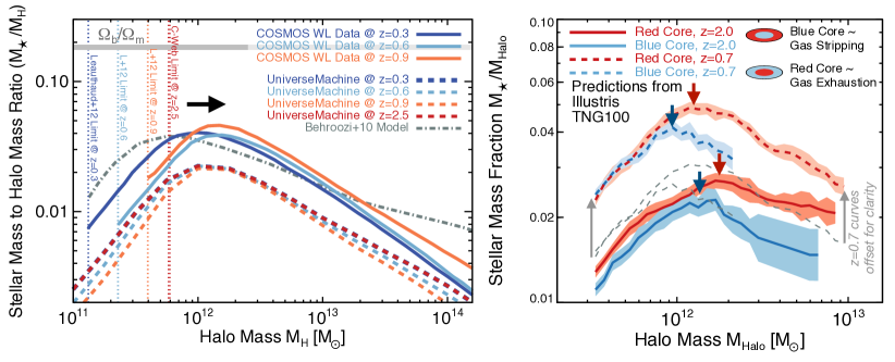
Directly measuring halo masses out to large galactocentric radii ( $\sim$ 1 Mpc, needed to probe the underlying dark matter) can be done either with galaxy-galaxy lensing (Brainerd et al., 1996) or using kinematic tracers like satellite galaxies (McKay et al., 2002). Given the sparsity of bright satellites beyond the local Universe and rarity of strongly-lensed galaxies, weak lensing (WL) is the only tool that can be used as a direct probe of halo masses for a large sample of galaxies across cosmic time (Sonnenfeld & Cautun, 2021). An innovative method combining galaxy clustering measures with HOD modeling and weak lensing was demonstrated by Leauthaud et al. (2011) and Leauthaud et al. (2012) using the COSMOS single band F814W Hubble imaging to measure SMHR evolution from $0.2<z<1.0$ at $M_{\star}>10^{10}$ M_⊙. These measurements are shown in the left panel of Figure 14.

COSMOS-Web’s 4-band NIRCam imaging spanning $>$ 0.5 deg², joined with the high quality 40 $+$ band imaging constraining galaxies’ masses and photometric redshifts in COSMOS (Weaver et al., 2022a, see also Figure 5), will be the best available dataset from which high resolution weak lensing mass mapping measurements can be done. This will involve a careful reconstruction of the PSF for each exposure in each filter and measurements of source centroids, shapes, and orientations. These measurements will then be combined with the best possible photometric redshifts to infer evolution in the SMHR (Leauthaud et al., 2007, 2011). Extending from $z\sim 1$ to $z\sim 2.5$ and to depths an order of magnitude deeper in halo mass at fixed redshift is enabled by the significant boost in spatially-resolved background and foreground sources where the weak lensing signal goes roughly as the square-root of the foreground source density multiplied by the background source density, $\propto\sqrt{N_{\rm fg}(z)}\sqrt{N_{\rm bg}(>z)}$ . The density of background sources will exceed 10 arcmin^-2 out to $z=4$ , with $\sim$ 110,000 sources at $z>2.5$ above 15 $\sigma$ , which is the necessary detection threshold for adequate shape recovery (Jee et al., 2017). Furthermore, these data will push that deep in each independent filter, thus will be the first wide, deep multi-band survey from space; simultaneous weak lensing measurement in multiple bands will both let us go even deeper and provide independent cross-checks of instrumental effects like the PSF calibration. Euclid and Hubble cannot observe at such long wavelengths (Lee et al., 2018) and Roman will not achieve such high resolution. Contiguous, high resolution NIR imaging from JWST in COSMOS-Web will thus serve as a much needed absolute calibration of the SMHR relation out to $z\sim 2.5$ that can be leveraged by other weak lensing surveys conducted on larger scales.

4.3.1 Evolution in the SMHR

Leauthaud et al. (2012) found unexpected evolution in the characteristic mass at which the SMHR is maximized (downsizing), in other words where the peak efficiency (around $\sim$ 10¹² M_⊙) evolves downward from $z\,\sim\,0.9$ to $z\,\sim\,0.3$ . Shuntov et al. (2022) similarly finds this downsizing trend with the COSMOS2020 catalog using clustering and constraints on the stellar mass function out to $z\sim 3$ . COSMOS-Web will significantly strengthen measurements to $z\sim 2.5$ with the important addition of weak lensing constraints, facilitating a re-calibration of hydrodynamical simulations and semi-analytic models that produce mock observables essential for much of cosmology and extragalactic astrophysics. This has important implications for how HOD modeling or abundance matching is used in the literature and how semi-analytic models and cosmological hydrodynamical simulations generate observables, on which much of extragalactic astrophysics relies.

Such weak lensing measurements rely on contiguous coverage over a large ( $\;\buildrel>\over{\sim}\;$ 0.5 deg²) area, otherwise they are substantially affected by edge effects (Mandelbaum et al., 2005; Massey et al., 2007b; Han et al., 2015). COSMOS-Web, with its large, deep, and contiguous coverage, will enable direct measurements of galaxies’ halo masses out to $z\sim 2.5$ down to $M_{\star}>$ few $\,\times 10^{9}$ M_⊙ (down to 10⁸ M_⊙ at $z\sim 1$ ), well beyond current data limitations (above $10^{10}$ M_⊙ at $z\lower 2.15277pt\hbox{$\;\buildrel<\over{\sim}\;$}1$ ) and future planned weak lensing measurements (e.g., from Euclid or Roman). Extending weak lensing measurements to $z\sim 2.5$ is essential for simulation calibration due to the significant evolution in galaxies’ properties (e.g., SFRs; Noeske et al., 2007; Whitaker et al., 2014) in the past 11 Gyr from $z=0-2.5$ .

The potential to extend SMHR constraints to higher redshifts is also possible using similar techniques to Shuntov et al. (2022). Such high redshifts and great mass depths can be reached due to the dramatic increase in the number of background sources for weak lensing and sources at all epochs that will have high-quality photometric redshifts.

4.3.2 Constraining the Dependency of the SMHR on Resolved Baryonic Observables

Given that COSMOS-Web data will be obtained in multiple filters, it will be the first sufficiently large dataset to test for alternate dependencies of resolved baryonic observables (e.g., color as a tracer of quenching mechanisms) on halo mass. This type of differential measurement with galaxy type is demonstrated by Tinker et al. (2013) out to $z\approx 1$ , who find that star-forming galaxies grow in lock-step with their dark matter halos, while quiescent galaxies have baryonic growth that is outpaced by dark matter growth. Higher redshifts can be reached by conducting the same experiment at longer wavelengths, boosting observed densities of high- $z$ sources. COSMOS-Web will push the limits of weak lensing’s direct measurement of halo masses to $z\sim 2.5$ with $M_{\star}>10^{10}$ M_⊙ such that halo masses can be independently constrained as a function of galaxy type over a significant portion of the Universe’s history.

Resolved color gradients in galaxies are thought to be the hallmark tracer of the quenching process. Bluer cores likely trace systems where cold gas has been stripped from the periphery (e.g., Meschin et al., 2014), while redder cores trace gas exhaustion, where gas at the galaxy core is not replenished (e.g., Kawata & Mulchaey, 2008; Tacchella et al., 2015). Flat color gradients are expected for galaxy collisions, in which the gas supply is consumed quickly with no preferred radial distribution (e.g., Springel, 2005; Sparre et al., 2015). While differential dust attenuation may complicate the interpretation of galaxies’ color gradients, some independent observations at long wavelengths could break the degeneracy (see the discussion later in § 5.3).

The right panel of Figure 14 illustrates the expected difference between the SMHR of bluer-cored galaxies and redder-cored galaxies. Do galaxies with different gradients show different evolution in their SMHRs? Cosmological simulations predict that similar SMHRs may point to the significant role of major galaxy mergers in the quenching process, while different SMHRs would point to feedback quenching mechanisms. At $z\lower 2.15277pt\hbox{$\;\buildrel<\over{\sim}\;$}2.5$ , our weak lensing measurements of halo masses for large samples can be directly compared with assertions that massive $>10^{10}$ M_⊙ galaxies evolve from star-forming to quenched in $\sim$ 100 Myr (e.g., Barro et al., 2013).

5 COSMOS-Web’s Impact on Other Topics

The breadth of scientific studies that COSMOS-Web may advance is extraordinary and impossible to anticipate in full. Below we describe some key ancillary science cases that could make significant strides given the layout and plans for the COSMOS-Web Treasury program. We emphasize that COSMOS-Web’s contribution to these areas will be powerful, though not made in isolation; much of the progress will be significantly aided by, if not fully dependent on, the legacy of data obtained in the COSMOS field from other observatories.

5.1 Galaxy Morphologies and Sizes to $z\sim 8$

Over the age of the Universe, galaxies have undergone dramatic morphological transformations. Today’s galaxies are a mix of well-formed spiral disk galaxies, ellipticals, and irregular galaxies and deep rest-frame optical images from Hubble have shown that the basis for what is known as the Hubble sequence was already in place by $z\sim 3$ (e.g., Wuyts et al., 2011; van der Wel et al., 2014; Kartaltepe et al., 2015b). Early JWST studies (e.g., Robertson et al. 2022b; Ferreira et al. 2022; Kartaltepe et al. 2022) are finding that galaxies at even higher redshifts have a wide diversity of morphologies, and a significant fraction already show evidence for disks and spheroids. However, a large fraction of galaxies at high redshift also have irregular morphologies, some of which may be signatures of galaxy mergers and interactions (e.g., Kartaltepe et al. 2012) and some may be indicative of other physical processes such as disk instabilities (e.g., Kereš et al. 2009; Genzel et al. 2011). In order to quantify the morphological transformation of galaxies from very early epochs to today, and understand the physical drivers responsible, large samples at high redshift are required.

COSMOS-Web will spatially resolve the rest-frame optical emission of tens of thousands of galaxies from $z=3-8$ , enabling a detailed morphological classification into spheroids/disks/irregulars and identification of interaction and merger signatures. These measurements will enable studies of morphological transformation as a function of environment and the relative roles of different physical processes responsible for enhanced star formation and black hole growth in the early universe. These large samples of morphology measurements will be essential training samples for machine learning algorithms (e.g., Snyder et al. 2019; Pearson et al. 2019; Hausen & Robertson 2020; Ćiprijanović et al. 2020; Rose et al. 2022) to classify galaxies, identify merger signatures, and identify unique morphologies that may otherwise be missed.

The evolution of galaxy sizes is also a useful tool for investigating the evolutionary history of galaxies and connecting the properties of today’s galaxies to their progenitors in the early universe. Over the past decade, a number of studies have found evidence for strong evolution in the optical/UV sizes of galaxies, with effective radii growing by a factor of 2–7 since $z\sim 2$ (e.g., van der Wel et al. 2008; Buitrago et al. 2008), suggesting that these massive galaxies have evolved through minor mergers in this time period (e.g., Naab et al. 2009; Bluck et al. 2012; Furlong et al. 2017). Both star-forming and quiescent populations of galaxies have been found to evolve in size, with samples of compact star forming (Barro et al., 2014a, b) and compact quiescent (e.g., Toft et al. 2007; van Dokkum et al. 2008; Bezanson et al. 2009; Barro et al. 2013) galaxies identified at cosmic noon. At even higher redshifts, $z=3-7$ , significant, though less steep, evolution has been found by a number of studies (e.g., van der Wel et al. 2014; Straatman et al. 2015; Shibuya et al. 2015; Whitney et al. 2019), and a range of physical mechanisms driving this evolution have been suggested, including major and minor mergers (e.g., Bluck et al. 2012; Wellons et al. 2016), rejuvenated star formation in the galaxy’s outer regions due to gas accretion (Conselice et al., 2013; Ownsworth et al., 2016; Dekel et al., 2020), quasar feedback (e.g., Fan et al. 2008; Dubois et al. 2016), and progenitor bias (van Dokkum & Franx, 2001).

Wellons et al. (2016) used Illustris to track the evolution of a sample of compact quiescent galaxies at $z\sim 2$ and found a diverse range of properties among their descendants, with very few remaining compact in the present day, in agreement with observations (Trujillo et al., 2009; Tortora et al., 2018; Scognamiglio et al., 2020). Most growth appears to be driven by the delivery of ex-situ mass and the impact of galaxy mergers and both are closely linked to a galaxy’s environment (Trujillo et al., 2007; Song et al., 2021). The progenitors of these compact quiescent galaxies themselves could have formed through gas-rich major mergers (e.g., Hopkins & Hernquist 2009; Barro et al. 2013; Wellons et al. 2015) or through clump migration (e.g., Dekel & Mandelker 2014). Additionally, the extension of the size-mass relation into the EoR is currently not well-constrained. UV measurements from the HUDF and CANDELS have found a range of sizes for these early galaxies (0.3–1 kpc, Oesch et al. 2010; Ono et al. 2013; Curtis-Lake et al. 2016) where mass is not very well measured given the limited scope of detection bands to the rest-frame UV.

Robust size measurements free from redshift bias are needed to adequately trace the evolution of galaxy sizes from the early Universe, which require deep rest-frame optical imaging of galaxies out into the EoR. In addition, the combination of analysis of galaxies’ rest-frame optical sizes can be compared to the sizes of their dust and gas reservoirs (e.g., Hodge & da Cunha, 2020) to further place constraints on the morphological transformation of galaxies across cosmic time.

5.2 Spatially Resolved Galaxy SEDs

The high resolution and deep images provided by COSMOS-Web NIRCam images will enable detailed pixel-by-pixel SED fitting of galaxies across a wide redshift range and down to lower stellar masses than has been possible to date (e.g., Wuyts et al. 2012; Jafariyazani et al. 2019; Abdurro’uf et al. 2021, 2023). The resulting mass, star formation rate, and dust attenuation maps can be used to study the star formation and quenching process in galaxies (e.g., Tacchella et al., 2015). The large number of sources in COSMOS-Web will enable the study of trends as a function of redshift, environment, and position relative to the star forming main sequence.

Mass maps that represent the overall resolved stellar mass of galaxies can be used for the morphological measurements described above. For example, Cibinel et al. (2015) show that morphological measurements using the mass maps of galaxies are better able to pick out features indicative of galaxy mergers than similar measures using standard light images. Similarly, precise size measurements can be made using mass maps in comparison with standard measurements (e.g., Suess et al. 2019; Mosleh et al. 2020). Clumps can be more easily identified using stellar mass maps and star formation rate maps can be used to quantify the growth of stellar mass in galaxies as a function of their morphology and environment.

5.3 Constraints on the Dust Attenuation Law

The dust attenuation law plays a crucial role in SED modeling for galaxies at all redshifts (Salim & Narayanan, 2020) but is heavily dependent on dust grain properties, total dust content, and dust geometry within galaxies’ interstellar media. Without direct constraints, most SED fitting routines blindly adopt one of a few common dust attenuation curves, for example that of the Milky Way galaxy (Cardelli et al., 1989) or the ‘Calzetti’ curve (Calzetti et al., 2000). Such blind adoption of an attenuation law that may or may not be applicable can result in substantial systemic biases introduced to extrapolated dust emission models, mass estimates, and star-formation rates (Mitchell et al., 2013; Laigle et al., 2019).

Well-sampled SEDs – from the rest-frame UV through the near-infrared – facilitate a direct measurement of the dust attenuation law (e.g., Kriek & Conroy, 2013). This is done by construction of broad SEDs that can then be fit to stellar population synthesis models with a range of dust attenuation law prescriptions to infer the best-fit solutions. The broader COSMOS survey includes 40 $+$ bands of coverage from the far-UV through the mid-infrared spanning both narrow and broad-band filters; such well-sampled SED coverage is sufficient to constrain some variation in the dust attenuation law, as has been measured in similar datasets (Pannella et al., 2015; Salmon et al., 2016; Reddy et al., 2018). However, a key limitation in constraining any possible evolution in the dust attenuation law comes from limited samples at higher redshifts, particularly at epochs where one might expect sufficiently different content and distribution of galaxies’ dust reservoirs. The added near-infrared (and mid-infrared) depth brought by COSMOS-Web will be crucial to dramatically increase the number of known, well-characterized galaxies out to $z\sim 4$ whose photometry can then be extracted across all COSMOS datasets to piece together large statistical samples of SEDs. These SEDs can, in turn, be used to infer redshift evolution in dust attenuation. A presumption of energy balance – where absorbed rest-frame UV emission is re-emitted at long wavelengths – can then be directly tested against deep submillimeter observations in the field, stacked using single-dish datasets (e.g., Oliver et al., 2012; Simpson et al., 2019) or individual constraints from galaxies observed by ALMA to much greater depths (e.g., the A3COSMOS project; Liu et al., 2019).

In addition to broad SED constraints, the ability to spatially resolve colors on kpc scales using NIRCam and Hubble/ACS imaging will allow direct measurement of the impact of dust geometry on galaxies’ integrated SEDs. This will be particularly useful for galaxies already detected by ALMA, of which we estimate there are $\sim$ 1000 (from ALMA Cycles 0-9) across the COSMOS-Web mosaic footprint. Dust geometry in complex ISM environments has long been a nuisance to SED fitting, as it often results in decoupling of the stellar and dust SEDs (Lower et al., 2022). COSMOS-Web will allow direct constraints on the relative degree of decoupling and its correlation to galaxy morphology as a function of color.

5.4 Finding & Characterizing Protoclusters

Galaxy clusters represent the most massive gravitationally bound structures in the Universe, and yet the history of their assembly is observationally uncertain. Galaxy clusters are typically found at $z\lower 2.15277pt\hbox{$\;\buildrel<\over{\sim}\;$}1.5$ thanks to thermal Bremsstrahlung radiation in the X-ray (Kravtsov & Borgani, 2012) or via the Sunyaev-Zel’dovich effect in the millimeter (Menanteau & Hughes, 2009; Vanderlinde et al., 2010) due to a hot $\sim$ 10⁷ K intracluster medium. A complete catalog of X-ray groups identified in COSMOS is compiled by Gozaliasl et al. (2019). However, the progenitors of galaxy clusters – called protoclusters – are observationally more elusive (Overzier, 2016). They have not yet virialized, thus their intracluster medium is not yet substantially heated to be distinguishable from the surrounding IGM. Before virialization, at $z\lower 2.15277pt\hbox{$\;\buildrel>\over{\sim}\;$}2$ , overdense environments are extended in large filaments that may span up to $\;\buildrel>\over{\sim}\;$ 10 comoving Mpc scales (Muldrew et al., 2015; Chiang et al., 2017). At $z\lower 2.15277pt\hbox{$\;\buildrel>\over{\sim}\;$}2$ , these physical scales span 10–30 arcminutes across, thus wide field-of-view surveys are needed to detect and characterize their spatial distribution.

Due to its large solid angle and sufficient depth to detect structures at $z>2$ , COSMOS has served as a primary observational field used to detect and analyze protoclusters at high redshifts (Yuan et al., 2014; Casey et al., 2015; Diener et al., 2015; Chiang et al., 2015; Hung et al., 2016). Such works have highlighted some of the challenges in constraining the forward evolution of such diffuse structures, where it is particularly difficult to constrain protoclusters’ halo masses, and yet total halo mass is crucial to the interpretation of their long-term evolutionary path (Sillassen et al., 2022). One particular structure, now dubbed “Hyperion,” lies in the center of the COSMOS field at $z\sim 2.5$ with an estimated $z=0$ halo mass exceeding 10¹⁵ M_⊙; a subcomponent of Hyperion has been discussed in the literature as a possible proto-virialized cluster core through the detection of associated extended X-ray emission (Wang et al., 2016, 2018b; Champagne et al., 2021). Its filamentary structures extend half a degree across and coincide well with the coverage of COSMOS-Web, which will allow a much richer mapping of its constituent galaxies at fainter luminosities. While spectroscopic follow-up will solve an essential piece of the puzzle in spatially mapping the full extent of known structures like Hyperion in COSMOS, the precise photometric redshifts provided by COSMOS-Web will dramatically improve the efficiency of follow-up. For example, reducing $\sigma_{\rm NMAD}(\Delta z/(1+z))$ from $\sim$ 0.06 to 0.03 for $\sim$ 27^th magnitude sources reduces the uncertainty in line-of-sight projected distance by a factor of $\sim$ 2 to $\sim$ 100 Mpc from $z\sim 2-5$ . While still significantly larger than the expected line-of-sight distances within protocluster environments, the increased precision will significantly improve the efficiency of follow-up spectroscopic campaigns targetting sources with photometric redshifts consistent with an overdensity of spectroscopic redshifts.

At higher redshifts, the prospect for discovering new protoclusters in COSMOS-Web is significant. Based on the $z\sim 0$ cluster mass function (e.g., Bahcall & Cen, 1993), we expect $\sim$ 30 structures between $2<z<8$ , $\sim$ 20 of which will be $4<z<8$ , that eventually collapse into $>5\times 10^{14}$ M_⊙ clusters at $z=0$ . Some of these we may have already found the first hints of based on ground-based data (e.g., Brinch et al., 2022), and the added depth and photometric redshift precision of COSMOS-Web will push the potential discovery space significantly. A more efficient mapping of such structures over an unbiased area will then allow more detailed investigations of the assembly history of protoclusters themselves (Casey, 2016).

5.5 Strong Lensing

The past three decades have seen the discovery of hundreds of galaxy-scale strong lenses (e.g., Bolton et al., 2008; Gavazzi et al., 2012; Rojas et al., 2021). COSMOS-Web will better resolve the 40 $+$ candidate strong lenses currently known in the COSMOS field from existing Hubble data and ground-based observations (Faure et al., 2008; Jackson, 2008), and has the potential to discover many more previously unknown galaxy-galaxy lenses due to the survey’s added depth in the near-infrared, sensitive to fainter, higher redshift background sources.

We perform a simple estimate of how many lenses will be in COSMOS-Web by first estimating the total number of galaxies acting as potential lenses. As intrinsically massive galaxies are needed to cleanly resolve the lensed system, we assume lensing galaxies are already part of the current COSMOS2020 catalog (Weaver et al., 2022a). We use the criterion $0.2<z_{\rm lens}<1.5$ , M ${}_{\star}>10^{9}\,$ M_⊙, and SFR $<10^{-1}\,$ M_⊙ yr^-1, resulting in a selection of $\sim$ 2 $\times$ 10⁵ galaxies. We take the median of the distribution of the stellar-to-halo mass relation from Shuntov et al. (2022) to define four mass bins: $9.0<\log M_{\star}<9.5$ ( $M_{\rm halo}\sim 2\times 10^{11}$ M_⊙), $9.5<\log M_{\star}<10.0$ ( $M_{\rm halo}\sim 4\times 10^{11}$ M_⊙), $10.0<\log M_{\star}<10.5$ ( $M_{\rm halo}\sim 7\times 10^{11}$ M_⊙), $10.5<\log M_{\star}<11.0$ ( $M_{\rm halo}\sim 1.2\times 10^{12}$ M_⊙). We estimate the surface on the sky where multiple imaging occurs ( $2<z_{\rm source}<13$ ) assuming lens mass profiles are isothermal spheres. We use the estimated number of $\sim$ 78 galaxies per arcmin² at $2<z<13$ drawn from UV luminosity functions (compiled by Behroozi et al., 2019). This calculation does not account for factors hindering the confirmation of lens candidates (e.g., confusion with spiral arms) and therefore may overestimate the number of lenses confirmed. To bring the number of lenses closer to realistic numbers, we perform the same calculation in the larger COSMOS field and rescale our results to the size of COSMOS-Web, assuming that 70 lenses are confirmed. This yields an expected $\sim$ 90 new lenses will be found in COSMOS-Web.

JWST’s unprecedented depth and resolution will lead to the discovery of the highest density of strong lenses per square degree, making it ideal for inferring line-of-sight shear with strong lenses (Fleury et al., 2021; Hogg et al., 2022) and complementing COSMOS-Web’s weak lensing analysis (see also Kuhn et al., 2021). Uniform multiband imaging of every strong lens will be available, overcoming challenges with deblending the lens and source light (Etherington et al., 2022). The highly magnified source galaxy population will allow for studies of high redshift galaxy formation (e.g., Swinbank et al., 2015) as well as detailed studies of the central mass profile of lensing galaxies (e.g., Koopmans et al., 2009; Nightingale et al., 2019; Shajib et al., 2021; Etherington et al., 2022) and dark matter contents (e.g., Vegetti et al., 2014; He et al., 2022).

5.6 Identifying Candidate Direct Collapse Black Holes

Direct Collapse Black Holes (DCBHs) have been proposed to resolve the mysterious quick growth of the Universe’s first supermassive black holes with $M_{\rm BH}\sim 10^{9}$ M_⊙ (Volonteri, 2010, 2012; Natarajan, 2011), found out to redshifts $z\sim 7.5$ (e.g., Wang et al., 2021). DCBHs are hypothesized to form black hole seeds of significant mass ( $\sim 10^{4-6}$ M_⊙; Shang et al., 2010; Johnson et al., 2012) from the primordial collapse of an atomic-cooling halo whereby strong Lyman-Werner photons could dissociate $H_{2}$ and prevent gas fragmentation, allowing the formation of DCBHs with significant mass and growth rates possibly exceeding Eddington rates (e.g., Volonteri & Rees, 2005; Alexander & Natarajan, 2014). Though no DCBH candidates have been directly confirmed, they are thought to have significant infrared through submillimeter emission, resulting in a steep, red near-infrared spectrum; they are also expected to have X-ray emission (Natarajan et al., 2017).

Pacucci et al. (2016) present two possible candidate DCBHs from CANDELS data in the GOODS-S area, both of which have photometric redshifts larger than $z\sim 6$ and robust X-ray detections as well as very steep infrared spectra. The improved depth of COSMOS-Web compared to CANDELS (out to 4.4 $\mu$ m or 7.7 $\mu$ m in the NIRCam mosaic or MIRI-covered subset) will allow more robust identification of fainter DCBH candidates with more robust photometric redshifts. The number density of the CANDELS-identified sources extrapolated to COSMOS-Web implies that we may find $\sim$ 20 such candidates in our full survey volume at $z>6$ . Such sources will then require spectroscopic follow-up with JWST to confirm their nature, assess their black hole masses, and to inform predictions for future deeper X-ray observations that may provide further confirmation.

5.7 Supermassive Black Hole - Galaxy Coevolution

COSMOS-Web will open new avenues to study AGN and quasars at high redshift. At $z>6$ , the black hole population with masses down to $10^{6}$ M_⊙ can be revealed through color-selection (see, for example, Goulding & Greene 2022) some of which may have resulted from an earlier DCBH event (see § 5.6). Using a semi-analytic model for the formation of the first galaxies and black holes (Trinca et al., 2022), we expect $\sim 50$ black holes within the COSMOS-Web volume that have $7<z<10$ and masses of 10 ${}^{6}-10^{8}$ M_⊙. With the spatial resolving power of JWST, morphologies can be decomposed into unresolved AGN emission and more diffuse host galaxy emission (Kocevski et al., 2022; Ding et al., 2022) on spatial scales of $\sim$ 1 kpc. With AGN-free host galaxy images, we can measure the mass relation between black holes and their hosts (M_BH vs. M_host) beyond $z\sim 3$ (Trakhtenbrot et al., 2015; Suh et al., 2020), carry out spatially-resolved studies of the stellar populations up to $z\sim 2$ , perform a quasar-galaxy cross correlation analysis (García-Vergara et al., 2017), and assess the influence of mergers (e.g., Mechtley et al., 2016; Shah et al., 2020). Furthermore, MIRI will aid in our ability to determine the demographics of the AGN population including the obscured population through detection of steep infrared (unresolved) sources with dominant torus emission.

5.8 Searches for $z>10$ Pair Instability Supernovae

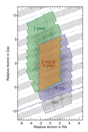
COSMOS-Web sits in unique parameter space, able to search for intrinsically rare phenomena at sensitivities beyond most wide-field surveys. Very high-redshift ( $z>5$ ) supernovae (SNe) in particular may provide a unique lens on the formation of the first massive stars by constraining the high-mass end of the Population III initial mass function. Such a first generation of stars is indeed thought to be top-heavy (Bromm et al., 1999, 2002). Ranging in mass from 100–260 M_⊙, such stars are most likely to die as pair-instability supernovae (PISNe; Heger & Woosley, 2002), which release up to 100 times more energy than Type Ia or Type II SNe (with intrinsic luminosities $\sim 10^{47-48}$ erg s^-1). Their extreme energy release is a result of electron-positron pair creation via thermal heating after the cessation of carbon burning in the core, leading to collapse and thermonuclear burning of O and Si; the energy released unbinds the star without leaving a remnant. Thanks to their luminosity and relative longevity (lengthened by $1+z$ time dilation) it is plausible to detect and identify PISNe brighter than NIR magnitudes $\sim$ 28 from $z=10-30$ in JWST NIRCam imaging surveys, particularly in the long wavelength channels. Whalen et al. (2013) present near-infrared light curves of PISNe from radiation hydrodynamical simulations, suggesting PISNe with $\;\buildrel>\over{\sim}\;$ 200 M_⊙ progenitors at $z\sim 15-30$ may remain detectable with F444W $\,<28$ (possibly as bright as $\sim$ 26^th magnitude) for 1-3 years, varying by $\sim$ 0.3 mags yr^-1. Hummel et al. (2012) present calculations of the expected number density of such JWST-detectable explosions at or below $\sim$ 0.02 arcmin^-2 at any given time at $z\lower 2.15277pt\hbox{$\;\buildrel>\over{\sim}\;$}10$ . This could result in $\sim$ 40 such events sitting within the COSMOS-Web NIRCam footprint.

The primary challenge in identifying PISNe candidates in COSMOS-Web will come from distinguishing them from high-redshift galaxies; thus, multi-epoch observations (conducted on roughly a yearly timescale) become critical to measuring the time-variable fading of the explosion. While most prior near-infrared datasets in COSMOS reach depths of only 25-26 mags (and are limited by the poor spatial resolution of Spitzer or ground-based UltraVISTA data), there may be a handful of exceptionally bright PISNe at $z>5$ whose transient nature can be constrained using existing observations on a $\sim$ 10 year cadence. Alternatively, over a smaller area, the CANDELS survey (Grogin et al., 2011; Koekemoer et al., 2011) conducted deep $\sim$ 28 imaging out to 1.6 $\mu$ m covering 200 arcmin² in late 2011 and early 2012; this provides a $\sim$ 10 year time baseline for potential $z\sim 5-12$ PISNe relative to COSMOS-Web observations detected in F150W (the redshift range limited directly by wavelength of deep imaging and the opacity of the IGM in absorbing photons shortward of 1216Å).

Out to higher redshifts, it may be possible to detect PISNe candidates out to $z\sim 30$ across a $\Delta t=1$ year timescale using imaging from the PRIMER JWST survey in conjunction with COSMOS-Web, as shown in Figure 15. Assuming there are no significant changes to the JWST long-range plan as of this writing, the PRIMER survey (GO #1837) will obtain half of their COSMOS NIRCam imaging in late 2022 covering an area $\sim$ 96 arcmin² out to F444W, and the other half in April 2023. Both PRIMER regions of the field will then be covered in late 2023 by COSMOS-Web, allowing a careful comparison of differential photometry for a potential handful of PISNe candidates brighter than $\sim$ 28. The total area with deep, $\sim$ 28^th magnitude $\sim$ 4.5 $\mu$ m multi-epoch JWST observations is $\sim$ 133 arcmin². Even with only a few detections, such PISNe candidates could potentially be extremely useful for constraining the nature of Population III stars formed shortly after the Big Bang.

5.9 Ultracool Halo Sub-Dwarf Stars

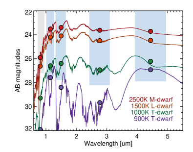
Ultracool dwarfs (late M-dwarfs through Y-dwarfs) are the most abundant stellar population by number and their prominent emission in the near-infrared implies that deep field surveys from JWST are prone to detect them to significant distances in the Galactic halo (Ryan & Reid, 2016). Indeed, mapping their number density to different distances in the outer halo may give unique constraints on the metal-poor initial mass function as well as the scale height of the Milky Way for low-mass objects (Burgasser et al., 2003; Carnero Rosell et al., 2019). Such discoveries are only enabled by deep near-infrared imaging, and given the wide area of COSMOS-Web, we anticipate finding of order $\sim$ 1000 such dwarfs across the field at various distances.

Figure 16 shows four ultracool dwarf templates from Saumon & Marley (2008) with varying effective temperature from 900 K, through the L-T transition at $\sim$ 1000 K up to late M-dwarfs at 2500 K. Models assume a 1000 m s^-2 surface gravity, consistent with expectation for older halo stars that would likely be found in extragalactic fields like COSMOS; no cloud cover is assumed below 1000 K, above which models with a moderate amount of cloud cover are adopted (Bowler, 2016). Significant absorption bands in ultracool T- and Y-dwarfs between 1.5–3.5 $\mu$ m, particularly at low $\;\buildrel<\over{\sim}\;$ 1000 K temperatures, lead to very distinct near-infrared colors from galaxies in NIRCam bands provided they are located at distances $\leq$ 1 kpc. For example, a recent late T-dwarf candidate was identified in JWST imaging of Abell 2744 at a distance of $\sim$ 600 pc by Nonino et al. (2022).

In addition to the science questions addressed by the detection of ultracool dwarfs, the population has also been a dominant contaminating source for searches of high-redshift galaxies, particularly samples of $z\sim 6-7$ sources due to their lack of emission shortward of $\sim$ 1 $\mu$ m. While Hubble imaging was limited to the shorter wavelengths, the long wavelength channels of NIRCam are of particular use in breaking the color degeneracies for distinguishing ultracool dwarfs from compact high-redshift galaxies. In addition, those ultracool dwarfs that would be more consistent with high-redshift galaxy colors are expected to be significantly brighter (peaking in density around $J\sim 24$ ; Ryan & Reid, 2016). Dwarfs at considerable distances $>$ 1 kpc, with apparent magnitudes fainter than $\sim$ 26 have the potential to contaminate $z\sim 6-7$ samples; however, their number density is expected to be relatively low relative to galaxies at similar magnitudes (fewer than $\sim$ 50 are expected across the COSMOS-Web mosaic fainter than $J\sim 26$ ).

6 Summary

We have presented the observational design and scientific goals of COSMOS-Web, the largest prime General Observer program in JWST’s Cycle 1 of observations. COSMOS-Web is a 0.54 deg² contiguous NIRCam survey imaged in four filters (F115W, F150W, F277W, and F444W) to depths of $\sim$ 27.5–28.2 magnitudes. In parallel, COSMOS-Web also includes 0.19 deg² non-contiguous MIRI imaging in one filter (F770W) to a depth of $\sim$ 25.3–26.0 magnitudes. COSMOS-Web is approximately 2.7 $\times$ larger than all other Cycle 1 JWST NIRCam deep field efforts combined and 3.5 $\times$ larger than the combined MIRI deep field coverage. The improvement in photometric redshift precision in COSMOS-Web will be substantial compared to the most recent catalogs compiled in the COSMOS field (Weaver et al., 2022a), with $<$ 5% errors on photometric redshifts down to magnitudes $\sim$ 27 in F277W.

The primary science goals of COSMOS-Web are threefold. First, COSMOS-Web will detect thousands of new galaxies within the Epoch of Reionization (EoR, $6\lower 2.15277pt\hbox{$\;\buildrel<\over{\sim}\;$}z\lower 2.15277pt\hbox{$\;\buildrel<\over{\sim}\;$}11$ ) and generate the largest number of galaxies at or above the knee of the UV luminosity function. Such intrinsically bright galaxies likely trace massive halos at early times at the nodes of the cosmic web. COSMOS-Web’s large area will allow a detailed mapping of the galaxy density field within the EoR on physical scales $\sim$ 150 Mpc across, sufficiently large to minimize cosmic variance by exceeding the size of the largest cosmic structures at these redshifts.

Second, COSMOS-Web aims to detect the Universe’s first massive quiescent galaxies that were likely in place between redshifts $4<z<6$ ; such galaxies mark the extreme limits of galaxy evolution at early times by building their stellar reservoirs at extraordinary rates (exceeding $\sim 10^{10}-10^{11}$ M_⊙ at $z>4$ ). We will be able to distinguish them from their dust star forming counterparts, study their morphologies and star formation histories, and thus place constraints on their progenitors.

Lastly, COSMOS-Web will measure the evolution in the stellar mass to halo mass relation (SMHR) from $0<z<2.5$ using weak gravitational lensing. The SMHR forms an essential anchor of cosmological simulations on large scales, and these data will extend its measurement from $z\sim 1$ to $z\sim 2.5$ in addition to allowing a detailed look at the SMHR by galaxy type and star-formation history (as probed by rest-frame optical colors and color gradients).

Beyond these core science goals, COSMOS-Web’s legacy value will extend to many subfields of extragalactic astronomy and beyond. We have summarized the potential impact of the survey on measuring galaxy morphologies, using spatially resolved SEDs to measure galaxy properties, placing constraints on the dust attenuation law, identifying and characterizing galaxy protoclusters, finding strong gravitational lenses, identifying direct collapse black hole candidates, studying the co-evolution of supermassive black holes and their host galaxies, searching for $z>10$ pair instability supernovae, and identifying ultracool sub-dwarf stars in the Milky Way’s halo. We hope the value of this survey continues to grow with time, as have many other deep-field observations before COSMOS-Web and JWST.

We thank the anonymous reviewer for helpful suggestions which greatly improved the manuscript. We thank the entire JWST team, including scientists, engineers, software developers, and the instrument and commissioning teams for making this amazing telescope a reality. We thank our program coordinator Christian Soto, our NIRCam reviewer Dan Coe, and our MIRI reviewer Stacey Bright for helping us to optimize our program and ensuring that the entire program is schedulable. We also thank the CEERS team for their quick release of simulations and observed data products, early testing and modification of the data reduction pipeline, and assisting with preparation for COSMOS-Web data reduction. Support for this work was provided by NASA through grant JWST-GO-01727 and HST-AR-15802 awarded by the Space Telescope Science Institute, which is operated by the Association of Universities for Research in Astronomy, Inc., under NASA contract NAS 5-26555. CMC thanks the National Science Foundation for support through grants AST-1814034 and AST-2009577 as well as the University of Texas at Austin College of Natural Sciences for support; CMC also acknowledges support from the Research Corporation for Science Advancement from a 2019 Cottrell Scholar Award sponsored by IF/THEN, an initiative of Lyda Hill Philanthropies. JSK acknowledges support from the College of Science and the Laboratory for Multiwavelength Astrophysics at the Rochester Institute of Technology. JSK acknowledges the important contributions to this paper, and the COSMOS-Web proposal, made by Shran and T’Pol, who attended every planning telecon and kept everyone’s spirits up in the early days of the COVID-19 pandemic. The Cosmic Dawn Center (DAWN) is funded by the Danish National Research Foundation under grant No. 140. JDR was supported by JPL, which is under a contract for NASA by Caltech. This research is also partly supported by the Centre National d’Etudes Spatiales (CNES). OI, CL, HHMCC acknowledge the funding of the French Agence Nationale de la Recherche for the project iMAGE (grant ANR-22-CE31-0007). BER was supported in part by NASA grant 80NSSC22K0814. MT and FG acknowledge the support from grant PRIN MIUR 2017 20173ML3WW_001. BT acknowledges support from the European Research Council (ERC) under the European Union’s Horizon 2020 research and innovation program (grant agreement 950533) and from the Israel Science Foundation (grant 1849/19) The authors acknowledge Research Computing at the Rochester Institute of Technology (2019) for providing computational resources and support for the work reported in this publication. This work used the CANDIDE computer system at the IAP supported by grants from the PNCG, CNES and the DIM-ACAV and maintained by S. Rouberol. We acknowledge use of the lux supercomputer at UC Santa Cruz, funded by NSF MRI grant AST1828315.

References

Abdurro’uf et al. (2021) Abdurro’uf, Lin, Y.-T., Wu, P.-F., & Akiyama, M. 2021, ApJS, 254, 15, doi: 10.3847/1538-4365/abebe2
Abdurro’uf et al. (2023) Abdurro’uf, Coe, D., Jung, I., et al. 2023, arXiv e-prints, arXiv:2301.02209, doi: 10.48550/arXiv.2301.02209
Abraham et al. (1996) Abraham, R. G., van den Bergh, S., Glazebrook, K., et al. 1996, ApJS, 107, 1, doi: 10.1086/192352
Aihara et al. (2022) Aihara, H., AlSayyad, Y., Ando, M., et al. 2022, PASJ, 74, 247, doi: 10.1093/pasj/psab122
Akeson et al. (2019) Akeson, R., Armus, L., Bachelet, E., et al. 2019, arXiv e-prints, arXiv:1902.05569. https://arxiv.org/abs/1902.05569
Alexander & Natarajan (2014) Alexander, T., & Natarajan, P. 2014, Science, 345, 1330, doi: 10.1126/science.1251053
Algera et al. (2020) Algera, H. S. B., van der Vlugt, D., Hodge, J. A., et al. 2020, ApJ, 903, 139, doi: 10.3847/1538-4357/abb77a
Arnouts et al. (2002) Arnouts, S., Moscardini, L., Vanzella, E., et al. 2002, MNRAS, 329, 355, doi: 10.1046/j.1365-8711.2002.04988.x
Arnouts et al. (2005) Arnouts, S., Schiminovich, D., Ilbert, O., et al. 2005, ApJ, 619, L43, doi: 10.1086/426733
Atek et al. (2022) Atek, H., Shuntov, M., Furtak, L. J., et al. 2022, arXiv e-prints, arXiv:2207.12338. https://arxiv.org/abs/2207.12338
Bahcall & Cen (1993) Bahcall, N., & Cen, R. 1993, ApJ, 407, L49, doi: 10.1086/186803
Bakx et al. (2022) Bakx, T. J. L. C., Zavala, J. A., Mitsuhashi, I., et al. 2022, arXiv e-prints, arXiv:2208.13642. https://arxiv.org/abs/2208.13642
Balogh et al. (2004) Balogh, M. L., Baldry, I. K., Nichol, R., et al. 2004, ApJ, 615, L101, doi: 10.1086/426079
Barro et al. (2013) Barro, G., Faber, S., Pérez-González, P., et al. 2013, ApJ, 765, 104, doi: 10.1088/0004-637X/765/2/104
Barro et al. (2014a) Barro, G., Faber, S. M., Pérez-González, P. G., et al. 2014a, ApJ, 791, 52, doi: 10.1088/0004-637X/791/1/52
Barro et al. (2014b) Barro, G., Trump, J. R., Koo, D. C., et al. 2014b, ApJ, 795, 145, doi: 10.1088/0004-637X/795/2/145
Becker et al. (2015) Becker, G., Bolton, J., Madau, P., et al. 2015, MNRAS, 447, 3402, doi: 10.1093/mnras/stu2646
Becker et al. (2018) Becker, G. D., Davies, F. B., Furlanetto, S. R., et al. 2018, ApJ, 863, 92, doi: 10.3847/1538-4357/aacc73
Beckwith et al. (2006) Beckwith, S., Stiavelli, M., Koekemoer, A., et al. 2006, AJ, 132, 1729, doi: 10.1086/507302
Behroozi et al. (2010) Behroozi, P., Conroy, C., & Wechsler, R. 2010, ApJ, 717, 379, doi: 10.1088/0004-637X/717/1/379
Behroozi et al. (2013) Behroozi, P., Wechsler, R., & Conroy, C. 2013, ApJ, 770, 57, doi: 10.1088/0004-637X/770/1/57
Behroozi et al. (2019) Behroozi, P., Wechsler, R. H., Hearin, A. P., & Conroy, C. 2019, MNRAS, 488, 3143, doi: 10.1093/mnras/stz1182
Behroozi et al. (2020) Behroozi, P., Conroy, C., Wechsler, R. H., et al. 2020, MNRAS, 499, 5702, doi: 10.1093/mnras/staa3164
Bezanson et al. (2009) Bezanson, R., van Dokkum, P. G., Tal, T., et al. 2009, ApJ, 697, 1290, doi: 10.1088/0004-637X/697/2/1290
Bluck et al. (2012) Bluck, A. F. L., Conselice, C. J., Buitrago, F., et al. 2012, ApJ, 747, 34, doi: 10.1088/0004-637X/747/1/34
Bolton et al. (2008) Bolton, A. S., Burles, S., Koopmans, L. V. E., et al. 2008, ApJ, 682, 964, doi: 10.1086/589327
Bouwens et al. (2006) Bouwens, R., Illingworth, G., Blakeslee, J., & Franx, M. 2006, ApJ, 653, 53, doi: 10.1086/498733
Bouwens et al. (2003) Bouwens, R., Illingworth, G., Rosati, P., et al. 2003, ApJ, 595, 589, doi: 10.1086/377477
Bouwens et al. (2015) Bouwens, R., Illingworth, G., Oesch, P., et al. 2015, ApJ, 803, 34, doi: 10.1088/0004-637X/803/1/34
Bouwens et al. (2021) Bouwens, R. J., Oesch, P. A., Stefanon, M., et al. 2021, AJ, 162, 47, doi: 10.3847/1538-3881/abf83e
Bowler (2016) Bowler, B. P. 2016, PASP, 128, 102001, doi: 10.1088/1538-3873/128/968/102001
Bowler et al. (2017) Bowler, R., Dunlop, J., McLure, R., & McLeod, D. 2017, MNRAS, 466, 3612, doi: 10.1093/mnras/stw3296
Bowler et al. (2020) Bowler, R., Jarvis, M., Dunlop, J., et al. 2020, MNRAS, doi: 10.1093/mnras/staa313
Bowler et al. (2014) Bowler, R., Dunlop, J., McLure, R., et al. 2014, MNRAS, 440, 2810, doi: 10.1093/mnras/stu449
Boyer et al. (2022) Boyer, M. L., Anderson, J., Gennaro, M., et al. 2022, arXiv e-prints, arXiv:2209.03348. https://arxiv.org/abs/2209.03348
Brainerd et al. (1996) Brainerd, T., Blandford, R., & Smail, I. 1996, ApJ, 466, 623, doi: 10.1086/177537
Brandt et al. (2000) Brandt, W. N., Laor, A., & Wills, B. J. 2000, ApJ, 528, 637, doi: 10.1086/308207
Brinch et al. (2022) Brinch, M., Greve, T. R., Weaver, J. R., et al. 2022, arXiv e-prints, arXiv:2210.17334. https://arxiv.org/abs/2210.17334
Brinchmann & Ellis (2000) Brinchmann, J., & Ellis, R. S. 2000, ApJ, 536, L77, doi: 10.1086/312738
Bromm et al. (1999) Bromm, V., Coppi, P. S., & Larson, R. B. 1999, ApJ, 527, L5, doi: 10.1086/312385
Bromm et al. (2002) —. 2002, ApJ, 564, 23, doi: 10.1086/323947
Buitrago et al. (2008) Buitrago, F., Trujillo, I., Conselice, C. J., et al. 2008, ApJ, 687, L61, doi: 10.1086/592836
Bunker et al. (2003) Bunker, A., Stanway, E., Ellis, R., McMahon, R., & McCarthy, P. 2003, MNRAS, 342, L47, doi: 10.1046/j.1365-8711.2003.06664.x
Bunker et al. (2023) Bunker, A. J., Saxena, A., Cameron, A. J., et al. 2023, arXiv e-prints, arXiv:2302.07256, doi: 10.48550/arXiv.2302.07256
Burgasser et al. (2003) Burgasser, A. J., Kirkpatrick, J. D., Burrows, A., et al. 2003, ApJ, 592, 1186, doi: 10.1086/375813
Calvi et al. (2016) Calvi, V., Trenti, M., Stiavelli, M., et al. 2016, ApJ, 817, 120, doi: 10.3847/0004-637X/817/2/120
Calzetti et al. (2000) Calzetti, D., Armus, L., Bohlin, R., et al. 2000, ApJ, 533, 682, doi: 10.1086/308692
Capak et al. (2007) Capak, P., Aussel, H., Ajiki, M., et al. 2007, ApJS, 172, 99, doi: 10.1086/519081
Capak et al. (2011) Capak, P., Mobasher, B., Scoville, N. Z., et al. 2011, ApJ, 730, 68, doi: 10.1088/0004-637X/730/2/68
Cardelli et al. (1989) Cardelli, J., Clayton, G., & Mathis, J. 1989, ApJ, 345, 245, doi: 10.1086/167900
Carnall et al. (2022) Carnall, A. C., McLeod, D. J., McLure, R. J., et al. 2022, arXiv e-prints, arXiv:2208.00986. https://arxiv.org/abs/2208.00986
Carnall et al. (2023) Carnall, A. C., McLure, R. J., Dunlop, J. S., et al. 2023, arXiv e-prints, arXiv:2301.11413, doi: 10.48550/arXiv.2301.11413
Carnero Rosell et al. (2019) Carnero Rosell, A., Santiago, B., dal Ponte, M., et al. 2019, MNRAS, 489, 5301, doi: 10.1093/mnras/stz2398
Casey (2016) Casey, C. 2016, ApJ, 824, 36. https://arxiv.org/abs/1603.04437
Casey et al. (2014) Casey, C., Narayanan, D., & Cooray, A. 2014, Phys. Rep., 541, 45, doi: 10.1016/j.physrep.2014.02.009
Casey et al. (2012) Casey, C., Berta, S., Béthermin, M., et al. 2012, ApJ, 761, 140, doi: 10.1088/0004-637X/761/2/140
Casey et al. (2015) Casey, C., Cooray, A., Capak, P., et al. 2015, ApJ, 808, L33, doi: 10.1088/2041-8205/808/2/L33
Casey et al. (2021) Casey, C. M., Zavala, J. A., Manning, S. M., et al. 2021, ApJ, 923, 215, doi: 10.3847/1538-4357/ac2eb4
Castellano et al. (2016) Castellano, M., Amorín, R., Merlin, E., et al. 2016, A&A, 590, A31, doi: 10.1051/0004-6361/201527514
Castellano et al. (2022) Castellano, M., Fontana, A., Treu, T., et al. 2022, ApJ, 938, L15, doi: 10.3847/2041-8213/ac94d0
Cecchi et al. (2019) Cecchi, R., Bolzonella, M., Cimatti, A., & Girelli, G. 2019, ApJ, 880, L14, doi: 10.3847/2041-8213/ab2c80
Chabrier (2003) Chabrier, G. 2003, PASP, 115, 763, doi: 10.1086/376392
Champagne et al. (2021) Champagne, J. B., Casey, C. M., Zavala, J. A., et al. 2021, ApJ, 913, 110, doi: 10.3847/1538-4357/abf4e6
Chiang et al. (2017) Chiang, Y.-K., Overzier, R. A., Gebhardt, K., & Henriques, B. 2017, ApJ, 844, L23, doi: 10.3847/2041-8213/aa7e7b
Chiang et al. (2015) Chiang, Y.-K., Overzier, R., Gebhardt, K., et al. 2015, ApJ, 808, 37, doi: 10.1088/0004-637X/808/1/37
Chisholm et al. (2020) Chisholm, J., Prochaska, J., Schaerer, D., Gazagnes, S., & Henry, A. 2020, MNRAS, 498, 2554, doi: 10.1093/mnras/staa2470
Christlein & Zabludoff (2005) Christlein, D., & Zabludoff, A. I. 2005, ApJ, 621, 201, doi: 10.1086/427427
Cibinel et al. (2015) Cibinel, A., Le Floc’h, E., Perret, V., et al. 2015, ApJ, 805, 181, doi: 10.1088/0004-637X/805/2/181
Ćiprijanović et al. (2020) Ćiprijanović, A., Snyder, G. F., Nord, B., & Peek, J. E. G. 2020, Astronomy and Computing, 32, 100390, doi: 10.1016/j.ascom.2020.100390
Civano et al. (2016) Civano, F., Marchesi, S., Comastri, A., et al. 2016, ApJ, 819, 62, doi: 10.3847/0004-637X/819/1/62
Conroy & Wechsler (2009) Conroy, C., & Wechsler, R. 2009, ApJ, 696, 620, doi: 10.1088/0004-637X/696/1/620
Conselice et al. (2000) Conselice, C., Bershady, M., & Jangren, A. 2000, ApJ, 529, 886, doi: 10.1086/308300
Conselice et al. (2013) Conselice, C. J., Mortlock, A., Bluck, A. F. L., Grützbauch, R., & Duncan, K. 2013, MNRAS, 430, 1051, doi: 10.1093/mnras/sts682
Cooper et al. (2008) Cooper, M., Tremonti, C., Newman, J., & Zabludoff, A. 2008, MNRAS, 390, 245, doi: 10.1111/j.1365-2966.2008.13714.x
Cooper et al. (2022) Cooper, O. R., Casey, C. M., Zavala, J. A., et al. 2022, ApJ, 930, 32, doi: 10.3847/1538-4357/ac616d
Cowley et al. (2018) Cowley, W., Caputi, K., Deshmukh, S., et al. 2018, ApJ, 853, 69, doi: 10.3847/1538-4357/aaa41d
Croton et al. (2006) Croton, D., Springel, V., White, S., et al. 2006, MNRAS, 365, 11, doi: 10.1111/j.1365-2966.2005.09675.x
Curtis-Lake et al. (2016) Curtis-Lake, E., McLure, R. J., Dunlop, J. S., et al. 2016, MNRAS, 457, 440, doi: 10.1093/mnras/stv3017
Curtis-Lake et al. (2022) Curtis-Lake, E., Carniani, S., Cameron, A., et al. 2022, arXiv e-prints, arXiv:2212.04568. https://arxiv.org/abs/2212.04568
Cutler et al. (2022) Cutler, S. E., Whitaker, K. E., Mowla, L. A., et al. 2022, ApJ, 925, 34, doi: 10.3847/1538-4357/ac341c
Daddi et al. (2007) Daddi, E., Alexander, D., Dickinson, M., et al. 2007, ApJ, 670, 173, doi: 10.1086/521820
D’Aloisio et al. (2018) D’Aloisio, A., McQuinn, M., Davies, F., & Furlanetto, S. 2018, MNRAS, 473, 560, doi: 10.1093/mnras/stx2341
Darvish et al. (2015) Darvish, B., Mobasher, B., Sobral, D., Scoville, N., & Aragon-Calvo, M. 2015, ApJ, 805, 121, doi: 10.1088/0004-637X/805/2/121
Davidzon et al. (2017) Davidzon, I., Ilbert, O., Laigle, C., et al. 2017, A&A, 605, A70, doi: 10.1051/0004-6361/201730419
Davis et al. (2018) Davis, B. L., Graham, A. W., & Cameron, E. 2018, ApJ, 869, 113, doi: 10.3847/1538-4357/aae820
Debackere et al. (2020) Debackere, S. N. B., Schaye, J., & Hoekstra, H. 2020, MNRAS, 492, 2285, doi: 10.1093/mnras/stz3446
Dekel & Mandelker (2014) Dekel, A., & Mandelker, N. 2014, MNRAS, 444, 2071, doi: 10.1093/mnras/stu1427
Dekel et al. (2020) Dekel, A., Lapiner, S., Ginzburg, O., et al. 2020, MNRAS, 496, 5372, doi: 10.1093/mnras/staa1713
Dickinson et al. (2004) Dickinson, M., Stern, D., Giavalisco, M., et al. 2004, ApJ, 600, L99, doi: 10.1086/381119
Diener et al. (2015) Diener, C., Lilly, S., Ledoux, C., et al. 2015, ApJ, 802, 31, doi: 10.1088/0004-637X/802/1/31
Dijkstra (2014) Dijkstra, M. 2014, PASA, 31, e040, doi: 10.1017/pasa.2014.33
Ding et al. (2022) Ding, X., Silverman, J. D., & Onoue, M. 2022, arXiv e-prints, arXiv:2209.03359. https://arxiv.org/abs/2209.03359
Donnan et al. (2022) Donnan, C. T., McLeod, D. J., Dunlop, J. S., et al. 2022, arXiv e-prints, arXiv:2207.12356. https://arxiv.org/abs/2207.12356
Donnari et al. (2019) Donnari, M., Pillepich, A., Nelson, D., et al. 2019, MNRAS, 485, 4817, doi: 10.1093/mnras/stz712
Drakos et al. (2022) Drakos, N. E., Villasenor, B., Robertson, B. E., et al. 2022, ApJ, 926, 194, doi: 10.3847/1538-4357/ac46fb
Dubois et al. (2016) Dubois, Y., Peirani, S., Pichon, C., et al. 2016, MNRAS, 463, 3948, doi: 10.1093/mnras/stw2265
Elbaz et al. (2007) Elbaz, D., Daddi, E., Le Borgne, D., et al. 2007, A&A, 468, 33, doi: 10.1051/0004-6361:20077525
Elvis et al. (2009) Elvis, M., Civano, F., Vignali, C., et al. 2009, ApJS, 184, 158, doi: 10.1088/0067-0049/184/1/158
Endsley et al. (2022a) Endsley, R., Stark, D. P., Whitler, L., et al. 2022a, arXiv e-prints, arXiv:2208.14999. https://arxiv.org/abs/2208.14999
Endsley et al. (2022b) Endsley, R., Stark, D. P., Lyu, J., et al. 2022b, arXiv e-prints, arXiv:2206.00018. https://arxiv.org/abs/2206.00018
Enia et al. (2022) Enia, A., Talia, M., Pozzi, F., et al. 2022, ApJ, 927, 204, doi: 10.3847/1538-4357/ac51ca
Etherington et al. (2022) Etherington, A., Nightingale, J. W., Massey, R., et al. 2022, MNRAS, 517, 3275, doi: 10.1093/mnras/stac2639
Euclid Collaboration et al. (2022) Euclid Collaboration, Scaramella, R., Amiaux, J., et al. 2022, A&A, 662, A112, doi: 10.1051/0004-6361/202141938
Faisst et al. (2016) Faisst, A., Capak, P., Davidzon, I., et al. 2016, ApJ, 822, 29, doi: 10.3847/0004-637X/822/1/29
Faisst et al. (2017) Faisst, A., Capak, P., Yan, L., et al. 2017, ArXiv e-prints. https://arxiv.org/abs/1708.07842
Fan et al. (2008) Fan, L., Lapi, A., De Zotti, G., & Danese, L. 2008, ApJ, 689, L101, doi: 10.1086/595784
Faure et al. (2008) Faure, C., Kneib, J.-P., Covone, G., et al. 2008, ApJS, 176, 19, doi: 10.1086/526426
Feldmann et al. (2016) Feldmann, R., Hopkins, P. F., Quataert, E., Faucher-Giguère, C.-A., & Kereš, D. 2016, MNRAS, 458, L14, doi: 10.1093/mnrasl/slw014
Ferreira et al. (2022) Ferreira, L., Conselice, C. J., Sazonova, E., et al. 2022, arXiv e-prints, arXiv:2210.01110. https://arxiv.org/abs/2210.01110
Finkelstein (2016) Finkelstein, S. 2016, PASA, 33, e037, doi: 10.1017/pasa.2016.26
Finkelstein et al. (2015) Finkelstein, S., Ryan, Jr., R., Papovich, C., et al. 2015, ApJ, 810, 71, doi: 10.1088/0004-637X/810/1/71
Finkelstein et al. (2022a) Finkelstein, S. L., Bagley, M. B., Arrabal Haro, P., et al. 2022a, arXiv e-prints, arXiv:2207.12474. https://arxiv.org/abs/2207.12474
Finkelstein et al. (2022b) Finkelstein, S. L., Bagley, M. B., Ferguson, H. C., et al. 2022b, arXiv e-prints, arXiv:2211.05792. https://arxiv.org/abs/2211.05792
Fleury et al. (2021) Fleury, P., Larena, J., & Uzan, J.-P. 2021, J. Cosmology Astropart. Phys, 2021, 024, doi: 10.1088/1475-7516/2021/08/024
Forrest et al. (2020) Forrest, B., Annunziatella, M., Wilson, G., et al. 2020, ApJ, 890, L1, doi: 10.3847/2041-8213/ab5b9f
Franco et al. (2018) Franco, M., Elbaz, D., Béthermin, M., et al. 2018, A&A, 620, A152, doi: 10.1051/0004-6361/201832928
Fujimoto et al. (2022a) Fujimoto, S., Finkelstein, S. L., Burgarella, D., et al. 2022a, arXiv e-prints, arXiv:2211.03896. https://arxiv.org/abs/2211.03896
Fujimoto et al. (2022b) Fujimoto, S., Brammer, G. B., Watson, D., et al. 2022b, Nature, 604, 261, doi: 10.1038/s41586-022-04454-1
Furlanetto et al. (2017) Furlanetto, S., Mirocha, J., Mebane, R., & Sun, G. 2017, MNRAS, 472, 1576, doi: 10.1093/mnras/stx2132
Furlong et al. (2017) Furlong, M., Bower, R. G., Crain, R. A., et al. 2017, MNRAS, 465, 722, doi: 10.1093/mnras/stw2740
García-Vergara et al. (2017) García-Vergara, C., Hennawi, J. F., Barrientos, L. F., & Rix, H.-W. 2017, ApJ, 848, 7, doi: 10.3847/1538-4357/aa8b69
Garel et al. (2021) Garel, T., Blaizot, J., Rosdahl, J., et al. 2021, MNRAS, 504, 1902, doi: 10.1093/mnras/stab990
Gavazzi et al. (2012) Gavazzi, R., Treu, T., Marshall, P. J., Brault, F., & Ruff, A. 2012, ApJ, 761, 170, doi: 10.1088/0004-637X/761/2/170
Genzel et al. (2011) Genzel, R., Newman, S., Jones, T., et al. 2011, ApJ, 733, 101, doi: 10.1088/0004-637X/733/2/101
Giacconi et al. (2002) Giacconi, R., Zirm, A., Wang, J., et al. 2002, ApJS, 139, 369, doi: 10.1086/338927
Giavalisco et al. (2004) Giavalisco, M., Ferguson, H. C., Koekemoer, A. M., et al. 2004, ApJ, 600, L93, doi: 10.1086/379232
Girelli et al. (2019) Girelli, G., Bolzonella, M., & Cimatti, A. 2019, A&A, 632, A80, doi: 10.1051/0004-6361/201834547
Glazebrook et al. (2017) Glazebrook, K., Schreiber, C., Labbé, I., et al. 2017, Nature, 544, 71, doi: 10.1038/nature21680
Gnedin & Kaurov (2014) Gnedin, N., & Kaurov, A. 2014, ApJ, 793, 30, doi: 10.1088/0004-637X/793/1/30
Gould et al. (2023) Gould, K. M. L., Brammer, G., Valentino, F., et al. 2023, arXiv e-prints, arXiv:2302.10934, doi: 10.48550/arXiv.2302.10934
Goulding & Greene (2022) Goulding, A. D., & Greene, J. E. 2022, arXiv e-prints, arXiv:2208.02822. https://arxiv.org/abs/2208.02822
Gozaliasl et al. (2019) Gozaliasl, G., Finoguenov, A., Tanaka, M., et al. 2019, MNRAS, 483, 3545, doi: 10.1093/mnras/sty3203
Grazian et al. (2015) Grazian, A., Fontana, A., Santini, P., et al. 2015, A&A, 575, A96, doi: 10.1051/0004-6361/201424750
Griffiths et al. (1996) Griffiths, R. E., Ratnatunga, K. U., Casertano, S., et al. 1996, in Examining the Big Bang and Diffuse Background Radiations, ed. M. C. Kafatos & Y. Kondo, Vol. 168, 219
Grogin et al. (2011) Grogin, N., Kocevski, D., Faber, S., et al. 2011, ApJS, 197, 35, doi: 10.1088/0067-0049/197/2/35
Gruppioni et al. (2020) Gruppioni, C., Béthermin, M., Loiacono, F., et al. 2020, A&A, 643, A8, doi: 10.1051/0004-6361/202038487
Guo et al. (2022) Guo, Y., Jogee, S., Finkelstein, S. L., et al. 2022, arXiv e-prints, arXiv:2210.08658. https://arxiv.org/abs/2210.08658
Hainline et al. (2011) Hainline, L., Blain, A., Smail, I., et al. 2011, ApJ, 740, 96, doi: 10.1088/0004-637X/740/2/96
Han et al. (2015) Han, J., Eke, V., Frenk, C., et al. 2015, MNRAS, 446, 1356, doi: 10.1093/mnras/stu2178
Harikane et al. (2022) Harikane, Y., Ouchi, M., Oguri, M., et al. 2022, arXiv e-prints, arXiv:2208.01612. https://arxiv.org/abs/2208.01612
Hashimoto et al. (2018) Hashimoto, T., Laporte, N., Mawatari, K., et al. 2018, Nature, 557, 392, doi: 10.1038/s41586-018-0117-z
Hasinger et al. (2018) Hasinger, G., Capak, P., Salvato, M., et al. 2018, ApJ, 858, 77, doi: 10.3847/1538-4357/aabacf
Hausen & Robertson (2020) Hausen, R., & Robertson, B. E. 2020, ApJS, 248, 20, doi: 10.3847/1538-4365/ab8868
He et al. (2022) He, Q., Robertson, A., Nightingale, J., et al. 2022, MNRAS, 511, 3046, doi: 10.1093/mnras/stac191
Heger & Woosley (2002) Heger, A., & Woosley, S. E. 2002, ApJ, 567, 532, doi: 10.1086/338487
Hoag et al. (2018) Hoag, A., Bradač, M., Brammer, G., et al. 2018, ApJ, 854, 39, doi: 10.3847/1538-4357/aaa9c2
Hodge & da Cunha (2020) Hodge, J. A., & da Cunha, E. 2020, Royal Society Open Science, 7, 200556, doi: 10.1098/rsos.200556
Hogg et al. (2022) Hogg, N. B., Fleury, P., Larena, J., & Martinelli, M. 2022, arXiv e-prints, arXiv:2210.07210. https://arxiv.org/abs/2210.07210
Hopkins & Hernquist (2009) Hopkins, P., & Hernquist, L. 2009, ApJ, 698, 1550, doi: 10.1088/0004-637X/698/2/1550
Hummel et al. (2012) Hummel, J. A., Pawlik, A. H., Milosavljević, M., & Bromm, V. 2012, ApJ, 755, 72, doi: 10.1088/0004-637X/755/1/72
Hung et al. (2016) Hung, C.-L., et al. 2016, ApJ, 1, 1
Hutter et al. (2021) Hutter, A., Dayal, P., Yepes, G., et al. 2021, MNRAS, doi: 10.1093/mnras/stab602
Ilbert et al. (2006) Ilbert, O., Arnouts, S., McCracken, H. J., et al. 2006, A&A, 457, 841, doi: 10.1051/0004-6361:20065138
Ilbert et al. (2010) Ilbert, O., Salvato, M., Le Floc’h, E., et al. 2010, ApJ, 709, 644, doi: 10.1088/0004-637X/709/2/644
Ilbert et al. (2013) Ilbert, O., McCracken, H., Le Fèvre, O., et al. 2013, A&A, 556, A55, doi: 10.1051/0004-6361/201321100
Jackson (2008) Jackson, N. 2008, MNRAS, 389, 1311, doi: 10.1111/j.1365-2966.2008.13629.x
Jafariyazani et al. (2019) Jafariyazani, M., Mobasher, B., Hemmati, S., et al. 2019, ApJ, 887, 204, doi: 10.3847/1538-4357/ab5526
Jee et al. (2017) Jee, M., Ko, J., Perlmutter, S., et al. 2017, ApJ, 847, 117, doi: 10.3847/1538-4357/aa88bc
Jiang et al. (2021) Jiang, L., Kashikawa, N., Wang, S., et al. 2021, Nature Astronomy, 5, 256, doi: 10.1038/s41550-020-01275-y
Johnson et al. (2012) Johnson, J. L., Whalen, D. J., Fryer, C. L., & Li, H. 2012, ApJ, 750, 66, doi: 10.1088/0004-637X/750/1/66
Kakiichi et al. (2016) Kakiichi, K., Dijkstra, M., Ciardi, B., & Graziani, L. 2016, MNRAS, 463, 4019, doi: 10.1093/mnras/stw2193
Kartaltepe et al. (2010) Kartaltepe, J., Sanders, D., Le Floc’h, E., et al. 2010, ApJ, 721, 98, doi: 10.1088/0004-637X/721/1/98
Kartaltepe et al. (2012) Kartaltepe, J., Dickinson, M., Alexander, D., et al. 2012, ApJ, 757, 23, doi: 10.1088/0004-637X/757/1/23
Kartaltepe et al. (2015a) Kartaltepe, J., Mozena, M., Kocevski, D., et al. 2015a, ApJS, 221, 11, doi: 10.1088/0067-0049/221/1/11
Kartaltepe et al. (2015b) Kartaltepe, J., Sanders, D., Silverman, J., et al. 2015b, ApJ, 806, L35, doi: 10.1088/2041-8205/806/2/L35
Kartaltepe et al. (2022) Kartaltepe, J. S., Rose, C., Vanderhoof, B. N., et al. 2022, arXiv e-prints, arXiv:2210.14713. https://arxiv.org/abs/2210.14713
Kashino et al. (2019) Kashino, D., Silverman, J. D., Sanders, D., et al. 2019, ApJS, 241, 10, doi: 10.3847/1538-4365/ab06c4
Kauffmann et al. (2004) Kauffmann, G., White, S. D. M., Heckman, T. M., et al. 2004, MNRAS, 353, 713, doi: 10.1111/j.1365-2966.2004.08117.x
Kauffmann et al. (2020) Kauffmann, O., Le Fèvre, O., Ilbert, O., et al. 2020, A&A, 640, A67, doi: 10.1051/0004-6361/202037450
Kauffmann et al. (2022) Kauffmann, O. B., Ilbert, O., Weaver, J. R., et al. 2022, arXiv e-prints, arXiv:2207.11740. https://arxiv.org/abs/2207.11740
Kawata & Mulchaey (2008) Kawata, D., & Mulchaey, J. 2008, ApJ, 672, L103, doi: 10.1086/526544
Kereš et al. (2009) Kereš, D., Katz, N., Fardal, M., Davé, R., & Weinberg, D. H. 2009, MNRAS, 395, 160, doi: 10.1111/j.1365-2966.2009.14541.x
Kocevski et al. (2022) Kocevski, D. D., Barro, G., McGrath, E. J., et al. 2022, arXiv e-prints, arXiv:2208.14480. https://arxiv.org/abs/2208.14480
Koekemoer et al. (2007) Koekemoer, A., Aussel, H., Calzetti, D., et al. 2007, ApJS, 172, 196, doi: 10.1086/520086
Koekemoer et al. (2011) Koekemoer, A., Faber, S., Ferguson, H., et al. 2011, ApJS, 197, 36, doi: 10.1088/0067-0049/197/2/36
Koopmans et al. (2009) Koopmans, L. V. E., Barnabe, M., Bolton, A., et al. 2009, in astro2010: The Astronomy and Astrophysics Decadal Survey, Vol. 2010, 159. https://arxiv.org/abs/0902.3186
Kravtsov et al. (2004) Kravtsov, A., Berlind, A., Wechsler, R., et al. 2004, ApJ, 609, 35, doi: 10.1086/420959
Kravtsov & Borgani (2012) Kravtsov, A., & Borgani, S. 2012, ARA&A, 50, 353, doi: 10.1146/annurev-astro-081811-125502
Kriek & Conroy (2013) Kriek, M., & Conroy, C. 2013, ApJ, 775, L16, doi: 10.1088/2041-8205/775/1/L16
Kriek et al. (2015) Kriek, M., Shapley, A. E., Reddy, N. A., et al. 2015, ApJS, 218, 15, doi: 10.1088/0067-0049/218/2/15
Kubo et al. (2018) Kubo, M., Tanaka, M., Yabe, K., et al. 2018, ApJ, 867, 1, doi: 10.3847/1538-4357/aae3e8
Kuhn et al. (2021) Kuhn, F. A., Birrer, S., Bruderer, C., Amara, A., & Refregier, A. 2021, J. Cosmology Astropart. Phys, 2021, 010, doi: 10.1088/1475-7516/2021/04/010
Labbe et al. (2022) Labbe, I., van Dokkum, P., Nelson, E., et al. 2022, arXiv e-prints, arXiv:2207.12446. https://arxiv.org/abs/2207.12446
Laigle et al. (2016) Laigle, C., McCracken, H., Ilbert, O., et al. 2016, ApJS, 224, 24, doi: 10.3847/0067-0049/224/2/24
Laigle et al. (2019) Laigle, C., Davidzon, I., Ilbert, O., et al. 2019, MNRAS, 486, 5104, doi: 10.1093/mnras/stz1054
Laporte et al. (2017) Laporte, N., Ellis, R., Boone, F., et al. 2017, ApJ, 837, L21, doi: 10.3847/2041-8213/aa62aa
Le Fèvre et al. (2015) Le Fèvre, O., Tasca, L. A. M., Cassata, P., et al. 2015, A&A, 576, A79, doi: 10.1051/0004-6361/201423829
Leauthaud et al. (2011) Leauthaud, A., Tinker, J., Behroozi, P., Busha, M., & Wechsler, R. 2011, ApJ, 738, 45, doi: 10.1088/0004-637X/738/1/45
Leauthaud et al. (2007) Leauthaud, A., Massey, R., Kneib, J.-P., et al. 2007, ApJS, 172, 219, doi: 10.1086/516598
Leauthaud et al. (2012) Leauthaud, A., Tinker, J., Bundy, K., et al. 2012, ApJ, 744, 159, doi: 10.1088/0004-637X/744/2/159
Lee et al. (2018) Lee, B., Chary, R.-R., & Wright, E. L. 2018, ApJ, 866, 157, doi: 10.3847/1538-4357/aadfd7
Lee et al. (2013) Lee, N., Sanders, D., Casey, C., et al. 2013, ApJ, 778, 131, doi: 10.1088/0004-637X/778/2/131
Legrand et al. (2019) Legrand, L., McCracken, H., Davidzon, I., et al. 2019, MNRAS, 486, 5468, doi: 10.1093/mnras/stz1198
Lilly et al. (2007) Lilly, S., Le Fèvre, O., Renzini, A., et al. 2007, ApJS, 172, 70, doi: 10.1086/516589
Lilly et al. (2009) Lilly, S., Le Brun, V., Maier, C., et al. 2009, ApJS, 184, 218, doi: 10.1088/0067-0049/184/2/218
Liu et al. (2019) Liu, D., Lang, P., Magnelli, B., et al. 2019, ApJS, 244, 40, doi: 10.3847/1538-4365/ab42da
Long et al. (2022) Long, A. S., Casey, C. M., Lagos, C. d. P., et al. 2022, arXiv e-prints, arXiv:2211.02072. https://arxiv.org/abs/2211.02072
Lotz et al. (2006) Lotz, J. M., Madau, P., Giavalisco, M., Primack, J., & Ferguson, H. C. 2006, ApJ, 636, 592, doi: 10.1086/497950
Lovell et al. (2022) Lovell, C. C., Wilkins, S. M., Thomas, P. A., et al. 2022, MNRAS, 509, 5046, doi: 10.1093/mnras/stab3221
Lowenthal et al. (1997) Lowenthal, J. D., Koo, D. C., Guzmán, R., et al. 1997, ApJ, 481, 673, doi: 10.1086/304092
Lower et al. (2022) Lower, S., Narayanan, D., Leja, J., et al. 2022, ApJ, 931, 14, doi: 10.3847/1538-4357/ac6959
Madau (1995) Madau, P. 1995, ApJ, 441, 18, doi: 10.1086/175332
Mandelbaum et al. (2006) Mandelbaum, R., Seljak, U., Kauffmann, G., Hirata, C., & Brinkmann, J. 2006, MNRAS, 368, 715, doi: 10.1111/j.1365-2966.2006.10156.x
Mandelbaum et al. (2005) Mandelbaum, R., Hirata, C., Seljak, U., et al. 2005, MNRAS, 361, 1287, doi: 10.1111/j.1365-2966.2005.09282.x
Mandelbaum et al. (2014) Mandelbaum, R., Rowe, B., Bosch, J., et al. 2014, ApJS, 212, 5, doi: 10.1088/0067-0049/212/1/5
Manning et al. (2022) Manning, S. M., Casey, C. M., Zavala, J. A., et al. 2022, ApJ, 925, 23, doi: 10.3847/1538-4357/ac366a
Maraston (2005) Maraston, C. 2005, MNRAS, 362, 799, doi: 10.1111/j.1365-2966.2005.09270.x
Mason et al. (2015) Mason, C. A., Trenti, M., & Treu, T. 2015, ApJ, 813, 21, doi: 10.1088/0004-637X/813/1/21
Massey et al. (2007a) Massey, R., Rhodes, J., Leauthaud, A., et al. 2007a, ApJS, 172, 239, doi: 10.1086/516599
Massey et al. (2007b) Massey, R., Rhodes, J., Ellis, R., et al. 2007b, Nature, 445, 286, doi: 10.1038/nature05497
McAlpine et al. (2016) McAlpine, S., Helly, J. C., Schaller, M., et al. 2016, Astronomy and Computing, 15, 72, doi: 10.1016/j.ascom.2016.02.004
McKay et al. (2002) McKay, T., Sheldon, E., Johnston, D., et al. 2002, ApJ, 571, L85, doi: 10.1086/341364
McLeod et al. (2016) McLeod, D. J., McLure, R. J., & Dunlop, J. S. 2016, MNRAS, 459, 3812, doi: 10.1093/mnras/stw904
McLure et al. (2013) McLure, R., Dunlop, J., Bowler, R., et al. 2013, MNRAS, 432, 2696, doi: 10.1093/mnras/stt627
McQuinn et al. (2007) McQuinn, M., Hernquist, L., Zaldarriaga, M., & Dutta, S. 2007, MNRAS, 381, 75, doi: 10.1111/j.1365-2966.2007.12085.x
Mechtley et al. (2016) Mechtley, M., Jahnke, K., Windhorst, R. A., et al. 2016, ApJ, 830, 156, doi: 10.3847/0004-637X/830/2/156
Menanteau & Hughes (2009) Menanteau, F., & Hughes, J. 2009, ApJ, 694, L136, doi: 10.1088/0004-637X/694/2/L136
Merlin et al. (2019) Merlin, E., Fortuni, F., Torelli, M., et al. 2019, MNRAS, 490, 3309, doi: 10.1093/mnras/stz2615
Meschin et al. (2014) Meschin, I., Gallart, C., Aparicio, A., et al. 2014, MNRAS, 438, 1067, doi: 10.1093/mnras/stt2220
Mitchell et al. (2013) Mitchell, P. D., Lacey, C. G., Baugh, C. M., & Cole, S. 2013, MNRAS, 435, 87, doi: 10.1093/mnras/stt1280
Mosleh et al. (2020) Mosleh, M., Hosseinnejad, S., Hosseini-ShahiSavandi, S. Z., & Tacchella, S. 2020, ApJ, 905, 170, doi: 10.3847/1538-4357/abc7cc
Mowla et al. (2019) Mowla, L., van Dokkum, P., Brammer, G., et al. 2019, ApJ, 880, 57
Muldrew et al. (2015) Muldrew, S., Hatch, N., & Cooke, E. 2015, MNRAS, 452, 2528, doi: 10.1093/mnras/stv1449
Muzzin et al. (2013) Muzzin, A., Marchesini, D., Stefanon, M., et al. 2013, ApJ, 777, 18, doi: 10.1088/0004-637X/777/1/18
Naab et al. (2009) Naab, T., Johansson, P. H., & Ostriker, J. P. 2009, ApJ, 699, L178, doi: 10.1088/0004-637X/699/2/L178
Naidu et al. (2020) Naidu, R. P., Tacchella, S., Mason, C. A., et al. 2020, ApJ, 892, 109, doi: 10.3847/1538-4357/ab7cc9
Naidu et al. (2022a) Naidu, R. P., Oesch, P. A., van Dokkum, P., et al. 2022a, arXiv e-prints, arXiv:2207.09434. https://arxiv.org/abs/2207.09434
Naidu et al. (2022b) Naidu, R. P., Oesch, P. A., Setton, D. J., et al. 2022b, arXiv e-prints, arXiv:2208.02794. https://arxiv.org/abs/2208.02794
Natarajan (2011) Natarajan, P. 2011, Bulletin of the Astronomical Society of India, 39, 145. https://arxiv.org/abs/1104.4797
Natarajan et al. (1998) Natarajan, P., Kneib, J.-P., Smail, I., & Ellis, R. S. 1998, ApJ, 499, 600, doi: 10.1086/305660
Natarajan et al. (2017) Natarajan, P., Pacucci, F., Ferrara, A., et al. 2017, ApJ, 838, 117, doi: 10.3847/1538-4357/aa6330
Nightingale et al. (2019) Nightingale, J. W., Massey, R. J., Harvey, D. R., et al. 2019, MNRAS, 489, 2049, doi: 10.1093/mnras/stz2220
Noeske et al. (2007) Noeske, K., Weiner, B., Faber, S., et al. 2007, ApJ, 660, L43, doi: 10.1086/517926
Nonino et al. (2022) Nonino, M., Glazebrook, K., Burgasser, A. J., et al. 2022, arXiv e-prints, arXiv:2207.14802. https://arxiv.org/abs/2207.14802
Oesch et al. (2010) Oesch, P., Bouwens, R., Illingworth, G., et al. 2010, ApJ, 709, L16, doi: 10.1088/2041-8205/709/1/L16
Oesch et al. (2013) —. 2013, ApJ, 773, 75, doi: 10.1088/0004-637X/773/1/75
Oesch et al. (2014) —. 2014, ApJ, 786, 108, doi: 10.1088/0004-637X/786/2/108
Oesch et al. (2015) Oesch, P., van Dokkum, P., Illingworth, G., et al. 2015, ApJ, 804, L30, doi: 10.1088/2041-8205/804/2/L30
Oesch et al. (2016) Oesch, P., Brammer, G., van Dokkum, P., et al. 2016, ApJ, 819, 129, doi: 10.3847/0004-637X/819/2/129
Oke & Gunn (1983) Oke, J. B., & Gunn, J. E. 1983, ApJ, 266, 713, doi: 10.1086/160817
Oliver et al. (2012) Oliver, S., Bock, J., Altieri, B., et al. 2012, MNRAS, 424, 1614, doi: 10.1111/j.1365-2966.2012.20912.x
Ono et al. (2013) Ono, Y., Ouchi, M., Curtis-Lake, E., et al. 2013, ApJ, 777, 155, doi: 10.1088/0004-637X/777/2/155
Ouchi et al. (2020) Ouchi, M., Ono, Y., & Shibuya, T. 2020, ARA&A, 58, 617, doi: 10.1146/annurev-astro-032620-021859
Overzier (2016) Overzier, R. 2016, A&A Rev., 24, 14, doi: 10.1007/s00159-016-0100-3
Ownsworth et al. (2016) Ownsworth, J. R., Conselice, C. J., Mundy, C. J., et al. 2016, MNRAS, 461, 1112, doi: 10.1093/mnras/stw1207
Pacucci et al. (2016) Pacucci, F., Ferrara, A., Grazian, A., et al. 2016, MNRAS, 459, 1432, doi: 10.1093/mnras/stw725
Pannella et al. (2015) Pannella, M., Elbaz, D., Daddi, E., et al. 2015, ApJ, 807, 141, doi: 10.1088/0004-637X/807/2/141
Papovich et al. (2001) Papovich, C., Dickinson, M., & Ferguson, H. C. 2001, ApJ, 559, 620, doi: 10.1086/322412
Pearson et al. (2019) Pearson, W. J., Wang, L., Alpaslan, M., et al. 2019, A&A, 631, A51, doi: 10.1051/0004-6361/201936337
Pentericci et al. (2018) Pentericci, L., Vanzella, E., Castellano, M., et al. 2018, ArXiv e-prints. https://arxiv.org/abs/1808.01847
Pillepich (2018) Pillepich, et. al.. 2018, MNRAS, 475, 648
Planck Collaboration et al. (2020) Planck Collaboration, Aghanim, N., Akrami, Y., et al. 2020, A&A, 641, A6, doi: 10.1051/0004-6361/201833910
Reddy et al. (2018) Reddy, N., Oesch, P., Bouwens, R., et al. 2018, ApJ, 853, 56, doi: 10.3847/1538-4357/aaa3e7
Rieke et al. (2022) Rieke, M. J., Kelly, D. M., Misselt, K., et al. 2022, arXiv e-prints, arXiv:2212.12069. https://arxiv.org/abs/2212.12069
Rigby et al. (2022) Rigby, J., Perrin, M., McElwain, M., et al. 2022, arXiv e-prints, arXiv:2207.05632. https://arxiv.org/abs/2207.05632
Roberts-Borsani et al. (2022) Roberts-Borsani, G., Treu, T., Chen, W., et al. 2022, arXiv e-prints, arXiv:2210.15639. https://arxiv.org/abs/2210.15639
Robertson et al. (2015) Robertson, B., Ellis, R., Furlanetto, S., & Dunlop, J. 2015, ApJ, 802, L19, doi: 10.1088/2041-8205/802/2/L19
Robertson (2010) Robertson, B. E. 2010, ApJ, 713, 1266, doi: 10.1088/0004-637X/713/2/1266
Robertson (2022) —. 2022, ARA&A, 60, 121, doi: 10.1146/annurev-astro-120221-044656
Robertson et al. (2022a) Robertson, B. E., Tacchella, S., Johnson, B. D., et al. 2022a, arXiv e-prints, arXiv:2212.04480. https://arxiv.org/abs/2212.04480
Robertson et al. (2022b) —. 2022b, arXiv e-prints, arXiv:2208.11456. https://arxiv.org/abs/2208.11456
Rochester Institute of Technology (2019) Rochester Institute of Technology. 2019, Research Computing Services
Rodighiero et al. (2022) Rodighiero, G., Bisigello, L., Iani, E., et al. 2022, arXiv e-prints, arXiv:2208.02825. https://arxiv.org/abs/2208.02825
Rodriguez-Gomez et al. (2016) Rodriguez-Gomez, V., Pillepich, A., Sales, L. V., et al. 2016, MNRAS, 458, 2371, doi: 10.1093/mnras/stw456
Rojas et al. (2021) Rojas, K., Savary, E., Clément, B., et al. 2021, arXiv e-prints, arXiv:2109.00014. https://arxiv.org/abs/2109.00014
Rose et al. (2022) Rose, C., Kartaltepe, J. S., Snyder, G. F., et al. 2022, arXiv e-prints, arXiv:2208.11164. https://arxiv.org/abs/2208.11164
Ryan & Reid (2016) Ryan, R. E., J., & Reid, I. N. 2016, AJ, 151, 92, doi: 10.3847/0004-6256/151/4/92
Salim & Narayanan (2020) Salim, S., & Narayanan, D. 2020, arXiv e-prints, arXiv:2001.03181. https://arxiv.org/abs/2001.03181
Salmon et al. (2016) Salmon, B., Papovich, C., Long, J., et al. 2016, ApJ, 827, 20, doi: 10.3847/0004-637X/827/1/20
Sanders & Mirabel (1996) Sanders, D., & Mirabel, I. 1996, ARA&A, 34, 749, doi: 10.1146/annurev.astro.34.1.749
Sanders et al. (2007) Sanders, D., Salvato, M., Aussel, H., et al. 2007, ApJS, 172, 86, doi: 10.1086/517885
Saumon & Marley (2008) Saumon, D., & Marley, M. S. 2008, ApJ, 689, 1327, doi: 10.1086/592734
Sawicki & Yee (1998) Sawicki, M., & Yee, H. K. C. 1998, AJ, 115, 1329, doi: 10.1086/300291
Scarlata et al. (2007) Scarlata, C., Carollo, C. M., Lilly, S., et al. 2007, ApJS, 172, 406, doi: 10.1086/516582
Schmidt et al. (2014) Schmidt, K., Treu, T., Trenti, M., et al. 2014, ApJ, 786, 57, doi: 10.1088/0004-637X/786/1/57
Schreiber et al. (2018) Schreiber, C., Glazebrook, K., Nanayakkara, T., et al. 2018, A&A, 618, A85, doi: 10.1051/0004-6361/201833070
Scognamiglio et al. (2020) Scognamiglio, D., Tortora, C., Spavone, M., et al. 2020, ApJ, 893, 4, doi: 10.3847/1538-4357/ab7db3
Scoville et al. (2007) Scoville, N., Aussel, H., Brusa, M., et al. 2007, ApJS, 172, 1, doi: 10.1086/516585
Scoville et al. (2013) Scoville, N., Arnouts, S., Aussel, H., et al. 2013, ApJS, 206, 3, doi: 10.1088/0067-0049/206/1/3
Seljak (2000) Seljak, U. 2000, MNRAS, 318, 203, doi: 10.1046/j.1365-8711.2000.03715.x
Shah et al. (2020) Shah, E. A., Kartaltepe, J. S., Magagnoli, C. T., et al. 2020, ApJ, 904, 107, doi: 10.3847/1538-4357/abbf59
Shahidi et al. (2020) Shahidi, A., Mobasher, B., Nayyeri, H., et al. 2020, ApJ, 897, 44, doi: 10.3847/1538-4357/ab96c5
Shajib et al. (2021) Shajib, A. J., Treu, T., Birrer, S., & Sonnenfeld, A. 2021, MNRAS, 503, 2380, doi: 10.1093/mnras/stab536
Shang et al. (2010) Shang, C., Bryan, G. L., & Haiman, Z. 2010, MNRAS, 402, 1249, doi: 10.1111/j.1365-2966.2009.15960.x
Shibuya et al. (2015) Shibuya, T., Ouchi, M., & Harikane, Y. 2015, ApJS, 219, 15, doi: 10.1088/0067-0049/219/2/15
Shuntov et al. (2022) Shuntov, M., McCracken, H. J., Gavazzi, R., et al. 2022, A&A, 664, A61, doi: 10.1051/0004-6361/202243136
Sillassen et al. (2022) Sillassen, N. B., Jin, S., Magdis, G. E., et al. 2022, A&A, 665, L7, doi: 10.1051/0004-6361/202244661
Silverman et al. (2015) Silverman, J., Kashino, D., Sanders, D., et al. 2015, ApJS, 220, 12, doi: 10.1088/0067-0049/220/1/12
Simpson et al. (2019) Simpson, J., Smail, I., Swinbank, A., et al. 2019, ApJ, 880, 43, doi: 10.3847/1538-4357/ab23ff
Simpson et al. (2020) Simpson, J. M., Smail, I., Dudzevičiūtė, U., et al. 2020, MNRAS, 495, 3409, doi: 10.1093/mnras/staa1345
Smolčić et al. (2017) Smolčić, V., Novak, M., Bondi, M., et al. 2017, A&A, 602, A1, doi: 10.1051/0004-6361/201628704
Snyder et al. (2019) Snyder, G. F., Rodriguez-Gomez, V., Lotz, J. M., et al. 2019, MNRAS, 486, 3702, doi: 10.1093/mnras/stz1059
Somerville et al. (2008) Somerville, R., Hopkins, P., Cox, T., Robertson, B., & Hernquist, L. 2008, MNRAS, 391, 481, doi: 10.1111/j.1365-2966.2008.13805.x
Song et al. (2021) Song, H., Laigle, C., Hwang, H. S., et al. 2021, MNRAS, 501, 4635, doi: 10.1093/mnras/staa3981
Song et al. (2016) Song, M., Finkelstein, S., Ashby, M., et al. 2016, ApJ, 825, 5, doi: 10.3847/0004-637X/825/1/5
Sonnenfeld & Cautun (2021) Sonnenfeld, A., & Cautun, M. 2021, A&A, 651, A18, doi: 10.1051/0004-6361/202140549
Sparre et al. (2015) Sparre, M., Hayward, C., Springel, V., et al. 2015, MNRAS, 447, 3548, doi: 10.1093/mnras/stu2713
Springel (2005) Springel, V. 2005, MNRAS, 364, 1105, doi: 10.1111/j.1365-2966.2005.09655.x
Stanway et al. (2003) Stanway, E. R., Bunker, A. J., & McMahon, R. G. 2003, MNRAS, 342, 439, doi: 10.1046/j.1365-8711.2003.06546.x
Stark (2016) Stark, D. 2016, ARA&A, 54, 761, doi: 10.1146/annurev-astro-081915-023417
Stefanon et al. (2019) Stefanon, M., Labbé, I., Bouwens, R., et al. 2019, arXiv e-prints. https://arxiv.org/abs/1902.10713
Steinhardt et al. (2016) Steinhardt, C. L., Capak, P., Masters, D., & Speagle, J. S. 2016, ApJ, 824, 21, doi: 10.3847/0004-637X/824/1/21
Straatman et al. (2014) Straatman, C. M., Labbé, I., Spitler, L. R., et al. 2014, ApJ, 783, L14, doi: 10.1088/2041-8205/783/1/L14
Straatman et al. (2015) Straatman, C. M. S., Labbé, I., Spitler, L. R., et al. 2015, ApJ, 808, L29, doi: 10.1088/2041-8205/808/1/L29
Suess et al. (2019) Suess, K. A., Kriek, M., Price, S. H., & Barro, G. 2019, ApJ, 877, 103, doi: 10.3847/1538-4357/ab1bda
Suh et al. (2020) Suh, H., Civano, F., Trakhtenbrot, B., et al. 2020, ApJ, 889, 32, doi: 10.3847/1538-4357/ab5f5f
Swinbank et al. (2015) Swinbank, A. M., Dye, S., Nightingale, J. W., et al. 2015, ApJ, 806, L17, doi: 10.1088/2041-8205/806/1/L17
Tacchella et al. (2015) Tacchella, S., Carollo, C. M., Renzini, A., et al. 2015, Science, 348, 314, doi: 10.1126/science.1261094
Talia et al. (2021) Talia, M., Cimatti, A., Giulietti, M., et al. 2021, ApJ, 909, 23, doi: 10.3847/1538-4357/abd6e3
Tanaka et al. (2019) Tanaka, M., Valentino, F., Toft, S., et al. 2019, ApJ, 885, L34, doi: 10.3847/2041-8213/ab4ff3
Thélie et al. (2022) Thélie, E., Aubert, D., Gillet, N., & Ocvirk, P. 2022, A&A, 658, A139, doi: 10.1051/0004-6361/202141748
Tinker et al. (2013) Tinker, J., Leauthaud, A., Bundy, K., et al. 2013, ApJ, 778, 93, doi: 10.1088/0004-637X/778/2/93
Tinker et al. (2010) Tinker, J. L., Robertson, B. E., Kravtsov, A. V., et al. 2010, ApJ, 724, 878, doi: 10.1088/0004-637X/724/2/878
Toft et al. (2007) Toft, S., van Dokkum, P., Franx, M., et al. 2007, ApJ, 671, 285, doi: 10.1086/521810
Tortora et al. (2018) Tortora, C., Napolitano, N. R., Roy, N., et al. 2018, MNRAS, 473, 969, doi: 10.1093/mnras/stx2390
Trakhtenbrot et al. (2015) Trakhtenbrot, B., Urry, C. M., Civano, F., et al. 2015, Science, 349, 168, doi: 10.1126/science.aaa4506
Trenti & Stiavelli (2008) Trenti, M., & Stiavelli, M. 2008, ApJ, 676, 767, doi: 10.1086/528674
Trinca et al. (2022) Trinca, A., Schneider, R., Maiolino, R., et al. 2022, MNRAS, doi: 10.1093/mnras/stac3768
Trujillo et al. (2009) Trujillo, I., Cenarro, A. J., de Lorenzo-Cáceres, A., et al. 2009, ApJ, 692, L118, doi: 10.1088/0004-637X/692/2/L118
Trujillo et al. (2007) Trujillo, I., Conselice, C., Bundy, K., et al. 2007, MNRAS, 382, 109, doi: 10.1111/j.1365-2966.2007.12388.x
Valentino et al. (2020) Valentino, F., Tanaka, M., Davidzon, I., et al. 2020, ApJ, 889, 93, doi: 10.3847/1538-4357/ab64dc
Valentino et al. (2023) Valentino, F., Brammer, G., Gould, K. M. L., et al. 2023, arXiv e-prints, arXiv:2302.10936, doi: 10.48550/arXiv.2302.10936
van der Vlugt et al. (2021) van der Vlugt, D., Algera, H. S. B., Hodge, J. A., et al. 2021, ApJ, 907, 5, doi: 10.3847/1538-4357/abcaa3
van der Wel et al. (2008) van der Wel, A., Holden, B. P., Zirm, A. W., et al. 2008, ApJ, 688, 48, doi: 10.1086/592267
van der Wel et al. (2014) van der Wel, A., Franx, M., van Dokkum, P. G., et al. 2014, ApJ, 788, 28, doi: 10.1088/0004-637X/788/1/28
van Dokkum & Franx (2001) van Dokkum, P. G., & Franx, M. 2001, ApJ, 553, 90, doi: 10.1086/320645
van Dokkum et al. (2008) van Dokkum, P. G., Franx, M., Kriek, M., et al. 2008, ApJ, 677, L5, doi: 10.1086/587874
Vanderlinde et al. (2010) Vanderlinde, K., Crawford, T., de Haan, T., et al. 2010, ApJ, 722, 1180, doi: 10.1088/0004-637X/722/2/1180
Vegetti et al. (2014) Vegetti, S., Koopmans, L. V. E., Auger, M. W., Treu, T., & Bolton, A. S. 2014, MNRAS, 442, 2017, doi: 10.1093/mnras/stu943
Volonteri (2010) Volonteri, M. 2010, A&A Rev., 18, 279, doi: 10.1007/s00159-010-0029-x
Volonteri (2012) —. 2012, Science, 337, 544, doi: 10.1126/science.1220843
Volonteri & Rees (2005) Volonteri, M., & Rees, M. J. 2005, ApJ, 633, 624, doi: 10.1086/466521
Wang et al. (2021) Wang, F., Yang, J., Fan, X., et al. 2021, ApJ, 907, L1, doi: 10.3847/2041-8213/abd8c6
Wang et al. (2018a) Wang, H., Mo, H. J., Chen, S., et al. 2018a, ApJ, 852, 31, doi: 10.3847/1538-4357/aa9e01
Wang et al. (2016) Wang, T., Elbaz, D., Daddi, E., et al. 2016, ApJ, 828, 56, doi: 10.3847/0004-637X/828/1/56
Wang et al. (2018b) —. 2018b, ArXiv e-prints. https://arxiv.org/abs/1810.10558
Wang et al. (2017) Wang, W.-H., Lin, W.-C., Lim, C.-F., et al. 2017, ApJ, 850, 37, doi: 10.3847/1538-4357/aa911b
Weaver et al. (2022a) Weaver, J. R., Kauffmann, O. B., Ilbert, O., et al. 2022a, ApJS, 258, 11, doi: 10.3847/1538-4365/ac3078
Weaver et al. (2022b) Weaver, J. R., Davidzon, I., Toft, S., et al. 2022b, arXiv e-prints, arXiv:2212.02512, doi: 10.48550/arXiv.2212.02512
Wechsler & Tinker (2018) Wechsler, R. H., & Tinker, J. L. 2018, ARA&A, 56, 435, doi: 10.1146/annurev-astro-081817-051756
Wellons et al. (2015) Wellons, S., Torrey, P., Ma, C.-P., et al. 2015, MNRAS, 449, 361, doi: 10.1093/mnras/stv303
Wellons et al. (2016) —. 2016, MNRAS, 456, 1030, doi: 10.1093/mnras/stv2738
Whalen et al. (2013) Whalen, D. J., Fryer, C. L., Holz, D. E., et al. 2013, ApJ, 762, L6, doi: 10.1088/2041-8205/762/1/L6
Whitaker et al. (2014) Whitaker, K., Franx, M., Leja, J., et al. 2014, ApJ, 795, 104, doi: 10.1088/0004-637X/795/2/104
Whitler et al. (2022) Whitler, L., Endsley, R., Stark, D. P., et al. 2022, arXiv e-prints, arXiv:2208.01599. https://arxiv.org/abs/2208.01599
Whitney et al. (2019) Whitney, A., Conselice, C. J., Bhatawdekar, R., & Duncan, K. 2019, ApJ, 887, 113, doi: 10.3847/1538-4357/ab53d4
Wilkins et al. (2017) Wilkins, S., Feng, Y., Di Matteo, T., et al. 2017, MNRAS, 469, 2517, doi: 10.1093/mnras/stx841
Wilkins et al. (2022) Wilkins, S. M., Vijayan, A. P., Lovell, C. C., et al. 2022, arXiv e-prints, arXiv:2204.09431. https://arxiv.org/abs/2204.09431
Williams et al. (2018) Williams, C. C., Curtis-Lake, E., Hainline, K. N., et al. 2018, ApJS, 236, 33, doi: 10.3847/1538-4365/aabcbb
Williams et al. (2022) Williams, H., Kelly, P. L., Chen, W., et al. 2022, arXiv e-prints, arXiv:2210.15699. https://arxiv.org/abs/2210.15699
Williams et al. (1996) Williams, R. E., Blacker, B., Dickinson, M., et al. 1996, AJ, 112, 1335, doi: 10.1086/118105
Williams et al. (2000) Williams, R. E., Baum, S., Bergeron, L. E., et al. 2000, AJ, 120, 2735, doi: 10.1086/316854
Wright et al. (2022) Wright, R. H., Sabatke, D., & Telfer, R. 2022, in Society of Photo-Optical Instrumentation Engineers (SPIE) Conference Series, Vol. 12180, Space Telescopes and Instrumentation 2022: Optical, Infrared, and Millimeter Wave, ed. L. E. Coyle, S. Matsuura, & M. D. Perrin, 121803P, doi: 10.1117/12.2632087
Wuyts et al. (2011) Wuyts, S., Förster Schreiber, N., van der Wel, A., et al. 2011, ApJ, 742, 96, doi: 10.1088/0004-637X/742/2/96
Wuyts et al. (2012) Wuyts, S., Förster Schreiber, N. M., Genzel, R., et al. 2012, ApJ, 753, 114, doi: 10.1088/0004-637X/753/2/114
Yoo et al. (2006) Yoo, J., Tinker, J., Weinberg, D., et al. 2006, ApJ, 652, 26, doi: 10.1086/507591
Yoo et al. (2009) Yoo, J., Weinberg, D., Tinker, J., Zheng, Z., & Warren, M. 2009, ApJ, 698, 967, doi: 10.1088/0004-637X/698/2/967
Yuan et al. (2014) Yuan, T., Nanayakkara, T., Kacprzak, G., et al. 2014, ApJ, 795, L20, doi: 10.1088/2041-8205/795/1/L20
Yung et al. (2020) Yung, L. Y. A., Somerville, R. S., Finkelstein, S. L., et al. 2020, MNRAS, 496, 4574, doi: 10.1093/mnras/staa1800
Yung et al. (2019) Yung, L. Y. A., Somerville, R. S., Popping, G., et al. 2019, MNRAS, 490, 2855, doi: 10.1093/mnras/stz2755
Zavala et al. (2021) Zavala, J. A., Casey, C. M., Manning, S. M., et al. 2021, ApJ, 909, 165, doi: 10.3847/1538-4357/abdb27
Zavala et al. (2022) Zavala, J. A., Buat, V., Casey, C. M., et al. 2022, arXiv e-prints, arXiv:2208.01816. https://arxiv.org/abs/2208.01816
Zheng et al. (2011) Zheng, Z., Cen, R., Weinberg, D., Trac, H., & Miralda-Escudé, J. 2011, ApJ, 739, 62, doi: 10.1088/0004-637X/739/2/62
Zheng & Weinberg (2007) Zheng, Z., & Weinberg, D. 2007, ApJ, 659, 1, doi: 10.1086/512151
Zitrin et al. (2015) Zitrin, A., Fabris, A., Merten, J., et al. 2015, ApJ, 801, 44, doi: 10.1088/0004-637X/801/1/44

\twocolumngrid

Appendix A Details of the COSMOS-Web Mosaic Visits

Here we provide detailed information on the 152 visits that comprise the COSMOS-Web mosaic. Table 6 lists all of the individual visits, their reference positions, and their position angles. The observation number is given as in the COSMOS-Web Proposal (#1727) opened in the Astronomer’s Proposal Tool (APT), and the visit name mirrors the target name in APT. The listed position angles are relative to the NIRCam frame (and differ from the V3 angle by 0.09^∘). The three visits that have position angles differing from the other visits in the mosaic are CWEBTILE-0-4, CWEBTILE-5-18, and CWEBTILE-7-15. Their angles are different due to availability of guide stars visible in the fine guidance sensor (FGS); no modification of their positions were required to keep the NIRCam mosaic contiguous. The positions as listed correspond to the reference position of NRCALL_FULL and sit at the reference point (V2,V3) = ( $-$ 0.32, $-$ 492.59) with 4TIGHT dither offsets taken $\pm$ 24 $\farcs$ 7 along V2 and $\pm$ 3 $\farcs$ 00 along V3. The relative positions of single visit coverage with respect to this reference point are shown in Figure 2.

\startlongtable

Table 6: COSMOS-Web Visit Positions

Obs No.	Visit Name	R.A.	Dec.	P.A.
1	CWEBTILE-0-0	09:59:42.539	$+$ 02:38:15.90	293
2	CWEBTILE-1-0	09:59:34.622	$+$ 02:32:49.78	293
39	CWEBTILE-2-0	09:59:26.708	$+$ 02:27:23.67	293
40	CWEBTILE-3-0	09:59:18.790	$+$ 02:21:57.55	293
77	CWEBTILE-4-0	09:59:10.876	$+$ 02:16:31.44	107
78	CWEBTILE-5-0	09:59:02.963	$+$ 02:11:05.33	107
115	CWEBTILE-6-0	09:58:55.049	$+$ 02:05:39.21	107
116	CWEBTILE-7-0	09:58:47.135	$+$ 02:00:13.10	107
3	CWEBTILE-0-1	09:59:50.742	$+$ 02:37:31.18	293
4	CWEBTILE-1-1	09:59:42.825	$+$ 02:32:05.06	293
41	CWEBTILE-2-1	09:59:34.907	$+$ 02:26:38.95	293
42	CWEBTILE-3-1	09:59:26.990	$+$ 02:21:12.83	293
79	CWEBTILE-4-1	09:59:19.076	$+$ 02:15:46.72	107
80	CWEBTILE-5-1	09:59:11.158	$+$ 02:10:20.60	107
117	CWEBTILE-6-1	09:59:03.245	$+$ 02:04:54.49	107
118	CWEBTILE-7-1	09:58:55.334	$+$ 01:59:28.37	107
5	CWEBTILE-0-2	09:59:58.942	$+$ 02:36:46.45	293
6	CWEBTILE-1-2	09:59:51.024	$+$ 02:31:20.34	293
43	CWEBTILE-2-2	09:59:43.107	$+$ 02:25:54.22	293
44	CWEBTILE-3-2	09:59:35.189	$+$ 02:20:28.11	293
81	CWEBTILE-4-2	09:59:27.272	$+$ 02:15:02.00	107
82	CWEBTILE-5-2	09:59:19.358	$+$ 02:09:35.88	107
119	CWEBTILE-6-2	09:59:11.444	$+$ 02:04:09.77	107
120	CWEBTILE-7-2	09:59:03.530	$+$ 01:58:43.65	107
7	CWEBTILE-0-3	10:00:07.141	$+$ 02:36:01.73	293
8	CWEBTILE-1-3	09:59:59.224	$+$ 02:30:35.62	293
45	CWEBTILE-2-3	09:59:51.306	$+$ 02:25:09.50	293
46	CWEBTILE-3-3	09:59:43.389	$+$ 02:19:43.39	293
83	CWEBTILE-4-3	09:59:35.471	$+$ 02:14:17.27	107
84	CWEBTILE-5-3	09:59:27.557	$+$ 02:08:51.16	107
121	CWEBTILE-6-3	09:59:19.640	$+$ 02:03:25.04	107
122	CWEBTILE-7-3	09:59:11.726	$+$ 01:57:58.93	107
9	CWEBTILE-0-4	10:00:15.341	$+$ 02:35:17.01	113 $\dagger$
10	CWEBTILE-1-4	10:00:07.423	$+$ 02:29:50.90	293
47	CWEBTILE-2-4	09:59:59.502	$+$ 02:24:24.78	293
48	CWEBTILE-3-4	09:59:51.584	$+$ 02:18:58.67	293
85	CWEBTILE-4-4	09:59:43.671	$+$ 02:13:32.55	107
86	CWEBTILE-5-4	09:59:35.753	$+$ 02:08:06.44	107
123	CWEBTILE-6-4	09:59:27.839	$+$ 02:02:40.32	107
124	CWEBTILE-7-4	09:59:19.926	$+$ 01:57:14.21	107
11	CWEBTILE-0-5	10:00:23.540	$+$ 02:34:32.29	293
12	CWEBTILE-1-5	10:00:15.623	$+$ 02:29:06.17	293
49	CWEBTILE-2-5	10:00:07.701	$+$ 02:23:40.059	293
50	CWEBTILE-3-5	09:59:59.784	$+$ 02:18:13.94	293
87	CWEBTILE-4-5	09:59:51.867	$+$ 02:12:47.83	107
88	CWEBTILE-5-5	09:59:43.949	$+$ 02:07:21.72	107
125	CWEBTILE-6-5	09:59:36.035	$+$ 02:01:55.60	107
126	CWEBTILE-7-5	09:59:28.121	$+$ 01:56:29.49	107
13	CWEBTILE-0-6	10:00:31.743	$+$ 02:33:47.57	293
14	CWEBTILE-1-6	10:00:23.822	$+$ 02:28:21.45	293
51	CWEBTILE-2-6	10:00:15.901	$+$ 02:22:55.34	293
52	CWEBTILE-3-6	10:00:07.983	$+$ 02:17:29.22	293
89	CWEBTILE-4-6	10:00:00.066	$+$ 02:12:03.11	107
90	CWEBTILE-5-6	09:59:52.148	$+$ 02:06:36.99	107
127	CWEBTILE-6-6	09:59:44.231	$+$ 02:01:10.88	107
128	CWEBTILE-7-6	09:59:36.317	$+$ 01:55:44.76	107
15	CWEBTILE-0-7	10:00:39.943	$+$ 02:33:02.85	293
16	CWEBTILE-1-7	10:00:32.021	$+$ 02:27:36.73	293
53	CWEBTILE-2-7	10:00:24.100	$+$ 02:22:10.62	293
54	CWEBTILE-3-7	10:00:16.179	$+$ 02:16:44.50	293
91	CWEBTILE-4-7	10:00:08.262	$+$ 02:11:18.39	107
92	CWEBTILE-5-7	10:00:00.344	$+$ 02:05:52.27	107
129	CWEBTILE-6-7	09:59:52.430	$+$ 02:00:26.16	107
130	CWEBTILE-7-7	09:59:44.513	$+$ 01:55:00.04	107
17	CWEBTILE-0-8	10:00:48.142	$+$ 02:32:18.12	293
18	CWEBTILE-1-8	10:00:40.217	$+$ 02:26:52.01	293
55	CWEBTILE-2-8	10:00:32.300	$+$ 02:21:25.89	293
56	CWEBTILE-3-8	10:00:24.379	$+$ 02:15:59.78	293
93	CWEBTILE-4-8	10:00:16.461	$+$ 02:10:33.66	107
94	CWEBTILE-5-8	10:00:08.544	$+$ 02:05:07.55	107
131	CWEBTILE-6-8	10:00:00.626	$+$ 01:59:41.44	107
132	CWEBTILE-7-8	09:59:52.709	$+$ 01:54:15.32	107
19	CWEBTILE-0-9	10:00:56.338	$+$ 02:31:33.40	293
20	CWEBTILE-1-9	10:00:48.417	$+$ 02:26:07.29	293
57	CWEBTILE-2-9	10:00:40.496	$+$ 02:20:41.17	293
58	CWEBTILE-3-9	10:00:32.578	$+$ 02:15:15.06	293
95	CWEBTILE-4-9	10:00:24.657	$+$ 02:09:48.94	107
96	CWEBTILE-5-9	10:00:16.740	$+$ 02:04:22.83	107
133	CWEBTILE-6-9	10:00:08.822	$+$ 01:58:56.71	107
134	CWEBTILE-7-9	10:00:00.905	$+$ 01:53:30.60	107
21	CWEBTILE-0-10	10:01:04.537	$+$ 02:30:48.68	293
22	CWEBTILE-1-10	10:00:56.616	$+$ 02:25:22.57	293
59	CWEBTILE-2-10	10:00:48.695	$+$ 02:19:56.45	293
60	CWEBTILE-3-10	10:00:40.774	$+$ 02:14:30.34	293
97	CWEBTILE-4-10	10:00:32.856	$+$ 02:09:04.22	107
98	CWEBTILE-5-10	10:00:24.935	$+$ 02:03:38.11	107
135	CWEBTILE-6-10	10:00:17.018	$+$ 01:58:11.99	107
136	CWEBTILE-7-10	10:00:09.104	$+$ 01:52:45.88	107
23	CWEBTILE-0-11	10:01:12.737	$+$ 02:30:03.96	293
24	CWEBTILE-1-11	10:01:04.816	$+$ 02:24:37.84	293
61	CWEBTILE-2-11	10:00:56.895	$+$ 02:19:11.73	293
62	CWEBTILE-3-11	10:00:48.973	$+$ 02:13:45.61	293
99	CWEBTILE-4-11	10:00:41.052	$+$ 02:08:19.50	107
100	CWEBTILE-5-11	10:00:33.135	$+$ 02:02:53.38	107
137	CWEBTILE-6-11	10:00:25.214	$+$ 01:57:27.27	107
138	CWEBTILE-7-11	10:00:17.300	$+$ 01:52:01.15	107
25	CWEBTILE-0-12	10:01:20.936	$+$ 02:29:19.24	293
26	CWEBTILE-1-12	10:01:13.011	$+$ 02:23:53.12	293
63	CWEBTILE-2-12	10:01:05.090	$+$ 02:18:27.01	293
64	CWEBTILE-3-12	10:00:57.169	$+$ 02:13:00.89	293
101	CWEBTILE-4-12	10:00:49.248	$+$ 02:07:34.78	107
102	CWEBTILE-5-12	10:00:41.331	$+$ 02:02:08.66	107
139	CWEBTILE-6-12	10:00:33.413	$+$ 01:56:42.55	107
140	CWEBTILE-7-12	10:00:25.496	$+$ 01:51:16.43	107
27	CWEBTILE-0-13	10:01:29.136	$+$ 02:28:34.51	293
28	CWEBTILE-1-13	10:01:21.211	$+$ 02:23:08.40	293
65	CWEBTILE-2-13	10:01:13.290	$+$ 02:17:42.28	293
66	CWEBTILE-3-13	10:01:05.365	$+$ 02:12:16.17	293
103	CWEBTILE-4-13	10:00:57.448	$+$ 02:06:50.06	107
104	CWEBTILE-5-13	10:00:49.526	$+$ 02:01:23.94	107
141	CWEBTILE-6-13	10:00:41.609	$+$ 01:55:57.83	107
142	CWEBTILE-7-13	10:00:33.691	$+$ 01:50:31.71	107
29	CWEBTILE-0-14	10:01:37.335	$+$ 02:27:49.79	293
30	CWEBTILE-1-14	10:01:29.410	$+$ 02:22:23.68	293
67	CWEBTILE-2-14	10:01:21.486	$+$ 02:16:57.56	293
68	CWEBTILE-3-14	10:01:13.564	$+$ 02:11:31.45	293
105	CWEBTILE-4-14	10:01:05.643	$+$ 02:06:05.33	107
106	CWEBTILE-5-14	10:00:57.722	$+$ 02:00:39.22	107
143	CWEBTILE-6-14	10:00:49.805	$+$ 01:55:13.10	107
144	CWEBTILE-7-14	10:00:41.887	$+$ 01:49:46.99	107
31	CWEBTILE-0-15	10:01:45.531	$+$ 02:27:05.07	293
32	CWEBTILE-1-15	10:01:37.606	$+$ 02:21:38.96	293
69	CWEBTILE-2-15	10:01:29.685	$+$ 02:16:12.84	293
70	CWEBTILE-3-15	10:01:21.760	$+$ 02:10:46.73	293
107	CWEBTILE-4-15	10:01:13.839	$+$ 02:05:20.61	107
108	CWEBTILE-5-15	10:01:05.918	$+$ 01:59:54.50	107
145	CWEBTILE-6-15	10:00:58.000	$+$ 01:54:28.38	107
146	CWEBTILE-7-15	10:00:50.079	$+$ 01:49:02.27	105 $\dagger$
33	CWEBTILE-0-16	10:01:53.730	$+$ 02:26:20.35	293
34	CWEBTILE-1-16	10:01:45.806	$+$ 02:20:54.23	293
71	CWEBTILE-2-16	10:01:37.881	$+$ 02:15:28.12	293
72	CWEBTILE-3-16	10:01:29.956	$+$ 02:10:02.00	293
109	CWEBTILE-4-16	10:01:22.035	$+$ 02:04:35.89	107
110	CWEBTILE-5-16	10:01:14.114	$+$ 01:59:09.77	107
147	CWEBTILE-6-16	10:01:06.196	$+$ 01:53:43.66	107
148	CWEBTILE-7-16	10:00:58.275	$+$ 01:48:17.55	107
35	CWEBTILE-0-17	10:02:01.930	$+$ 02:25:35.63	293
36	CWEBTILE-1-17	10:01:54.001	$+$ 02:20:09.51	293
73	CWEBTILE-2-17	10:01:46.077	$+$ 02:14:43.40	293
74	CWEBTILE-3-17	10:01:38.156	$+$ 02:09:17.28	293
111	CWEBTILE-4-17	10:01:30.231	$+$ 02:03:51.17	107
112	CWEBTILE-5-17	10:01:22.310	$+$ 01:58:25.05	107
149	CWEBTILE-6-17	10:01:14.392	$+$ 01:52:58.94	107
150	CWEBTILE-7-17	10:01:06.471	$+$ 01:47:32.82	107
37	CWEBTILE-0-18	10:02:10.126	$+$ 02:24:50.90	293
38	CWEBTILE-1-18	10:02:02.201	$+$ 02:19:24.79	293
75	CWEBTILE-2-18	10:01:54.276	$+$ 02:13:58.67	293
76	CWEBTILE-3-18	10:01:46.351	$+$ 02:08:32.56	293
113	CWEBTILE-4-18	10:01:38.430	$+$ 02:03:06.45	107
114	CWEBTILE-5-18	10:01:30.505	$+$ 01:57:40.33	104.5 $\dagger$
151	CWEBTILE-6-18	10:01:22.588	$+$ 01:52:14.22	107
152	CWEBTILE-7-18	10:01:14.667	$+$ 01:46:48.10	107

Note. — The position angle (P.A.) of the visit is specified in the last

column; only three visits have non-standard position angles caused

by guide star catalog limitations and they are marked with a $\dagger$ . We

quote 0 $\farcs$ 01 accuracy on tile positions.