Local Magnification for Data and Feature Augmentation

Abstract

In recent years, many data augmentation techniques have been proposed to increase the diversity of input data and reduce the risk of overfitting on deep neural networks. In this work, we propose an easy-to-implement and model-free data augmentation method called Local Magnification (LOMA). Different from other geometric data augmentation methods that perform global transformations on images, LOMA generates additional training data by randomly magnifying a local area of the image. This local magnification results in geometric changes that significantly broaden the range of augmentations while maintaining the recognizability of objects. Moreover, we extend the idea of LOMA and random cropping to the feature space to augment the feature map, which further boosts the classification accuracy considerably. Experiments show that our proposed LOMA, though straightforward, can be combined with standard data augmentation to significantly improve the performance on image classification and object detection. And further combination with our feature augmentation techniques, termed LOMA_IF&FO, can continue to strengthen the model and outperform advanced intensity transformation methods for data augmentation.

1 Introduction

Convolutional neural networks (CNNs) have achieved broad success over a variety of computer vision tasks, including image classification [20, 28, 9], object detection [13, 25], and semantic segmentation [23, 3]. However, overfitting often occurs during training and reduces model performance. A widely used technique to combat this problem is data augmentation, which expands the set of valid training data and improves the generalization of neural networks.

Mainstream image augmentation methods can be split into three categories [33], namely model-free, model-based, and optimization-based. Among them, model-free methods such as Cutout [8], Hide and Seek [29], Random Erasing [38], and GridMask [4] have been especially popular due to their relative simplicity and effectiveness. As illustrated in Fig. 1, model-free data augmentations mainly focus on occluding some of the image content via intensity transformations so that the CNNs can be pushed to learn more robust features. However, when an essential portion of an image is occluded, the image label may become ambiguous. For instance, when the data augmentation completely masks valuable objects in the input image, the image data becomes noisy and harmful to the training of CNNs.

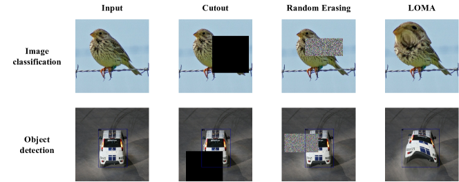
Figure 1: Illustration of augmented images by various methods, including Cutout, Random Erasing and our Local Magnification (LOMA).

To avoid such label ambiguity in model-free data augmentation, we introduce a new data augmentation method, termed Local Magnification (LOMA). Unlike other geometric augmentations that are based on global geometric transformations, such as affine transformations, elastic distortions [27], random cropping [20], and random flipping [28], LOMA only magnifies a local portion of the image to generate the augmentation, making some local features more prominent.

In the physical world, occlusion can happen where some portion of a scene is occluded by other objects, while our LOMA can also occur like when a person uses a magnifier on an input image to facilitate focusing on some details. Another case is that cars can be severely deformed in a traffic accident yet still be well recognized. Also, human faces can be exaggeratedly distorted in funhouse curved mirrors but still be recognized from the distorted images by people.

In network training, LOMA is applied to each image of a mini-batch with a fixed probability. First, a magnification center is randomly located on each selected image, and a radius is determined within a specified range. Then, LOMA calculates new horizontal and vertical coordinates for all the pixels located within a neighborhood of the magnification center that is defined by the radius and a preset deformation shape. These pixels are moved accordingly to obtain the new image, as shown for two preset deformation shapes (rhombus and ellipse) in Fig. 2. Although this procedure may discard a small portion of the pixels, the number of discarded pixels is much less than that of intensity transformation methods based on occlusion. In addition, some augmented images will have apparent dislocations at the boundaries of the augmented region, which cannot be achieved by intensity transformation. We argue that these deformations and dislocations increase the diversity of the training data while maintaining the apparent image labels, providing challenging yet effective training data that goes well beyond the standard augmentations.

We additionally extend the idea of our local magnification as well as the standard random cropping to augment feature maps in the feature space. The former is called LOMA on the Feature Map, and the latter is called FeatureMap Offset (FO). We abbreviate the joint use of LOMA and LOMA on the Feature Map as LOMA_IF (LOMA in the Image space and Feature space). For FeatureMap Offset, it offsets the feature map output at an intermediate layer of the network with a certain probability and then passes it to the subsequent layer.

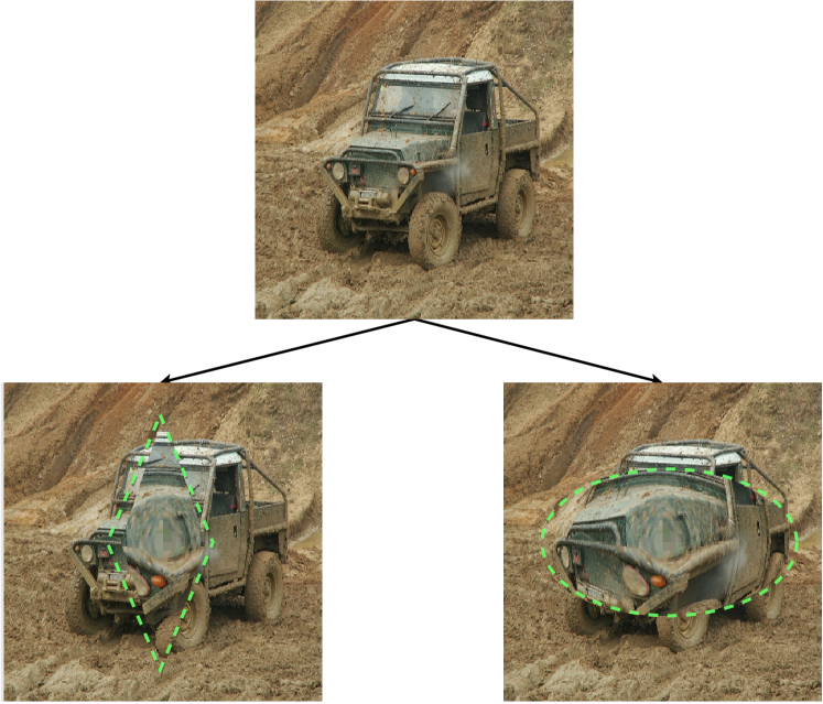
Figure 2: Examples of LOMA for two preset deformation shapes (rhombus and ellipse).

Our main contributions can be summarized as follows:

• We propose a model-free data augmentation method based on local geometric transformations called Local Magnification (LOMA). It is a lightweight method that does not require additional parameters to learn and can be easily plugged into the training of various CNNs.

• The proposed LOMA improves the baseline (standard augmentation) for image classification on the CIFAR and ImageNet benchmark datasets and for object detection on the PASCAL VOC benchmark dataset. LOMA can be combined with standard data augmentation to further boost the performance.

• We extend the idea of LOMA and random cropping to the feature space. The incorporation of our final method, termed LOMA_IF&FO, can further boost performance and outperform two advanced intensity transformation data augmentation methods, Cutout [8] and Random Erasing [38].

2 Related Work

2.1 Data Augmentation

In recent years, many data augmentation techniques have been proposed to address the overfitting issue that arises when training convolutional neural networks (CNNs) [33]. Existing data augmentation methods can be categorized into three groups, namely model-free, model-based, and optimizing policy-based.

Model-based approaches attempt to augment the training dataset with images produced by Generative Networks. Antoniou et al. [1] use a generative model called DCGAN to take data from a source domain and generalize it to generate other within-class data. Huang et al. [17] propose a structure-aware image-to-image translation network called AugGAN to learn the joint distribution of the two domains and find transformations between them. Xu et al. [32] adopt the self-supervised masked autoencoder to generate distorted views of the input images as augmented images.

Optimizing policy-based image augmentation strategies seek to find the optimal combination policy of multiple data augmentation methods through reinforcement learning or adversarial learning. The most representative work is AutoAugment [5], which has demonstrated powerful performance on various benchmarks but spends much time searching for policies. There are many follow-up improvements, such as Fast AutoAugment [22], Adversarial AutoAugment [37], RandAugment [6], Faster AutoAugment [15], and TeachAugment [31].

Most relevant to our work are model-free data augmentation methods. In addition to methods that process multiple images to obtain new samples, such as Mixup [36], CutMix [34], and PuzzleMix [18], there are single-image augmentation strategies, which can be divided into three branches: geometric transformation, color image processing, and intensity transformation. Color image processing methods perturb the color of the input image by transforming the color of pixels within the training data. In the intensity transformation methods, DeVries and Taylor [8] propose Cutout, which uses a square fixed-size mask to randomly occlude a portion of the image and fill it with uniform pixels. Zhong et al. [38] propose Random Erasing, which uses random pixel values to form a rectangular mask. To establish a good balance between deletion and the preservation of regional information on the images, Chen et al. [4] introduce GridMask, which randomly removes non-adjacent image patches. The above methods all perform some occlusion so as to encourage the network to focus more on complementary and less prominent features [8]. Instead of blocking a portion of the image directly, our method alters the position of pixels to magnify a local area of the image, making it more prominent and helping the network to focus more on these local features. As the local region is located randomly, the network can learn to generalize to more extensive variations of the original image.

2.2 Regularization

Another effective approach to address the overfitting issue in CNNs is by regularization in the feature space. Dropout [30] randomly drops units and their connections from the neural network during training. Follow-ups to Dropout contain many improvements, such as DropBlock [12] which occludes continuous regions on the feature map. Another idea is to exchange some components of the two feature maps. For example, PatchUp [11] mixes consecutive feature blocks in the feature space. MoEx [21] forces the model to improve robustness by randomly replacing the moments of the feature map of one training sample with those of another and interpolating the labels. These methods can also be regarded as augmentations in the feature space. Thereby, we apply our LOMA in the feature space as another form of regularization, and we further consider porting standard data augmentations, namely random cropping and random flipping, to the feature space as well. As random flipping in the image space and feature space have similar effects, we only adopt random cropping in the feature space and refer to this new method as FeatureMap Offset (FO).

2.3 Standard Data Augmentation Suite

The two most successful data augmentation techniques for training CNNs are the geometric transformations of random cropping [20] and random flipping [28]. Through these two types of augmentations, the diversity of training samples is increased. Unlike random cropping and random flipping which perform a global transformation of an image, LOMA can be regarded as a local geometric transformation because it does not alter the overall structure of the image. Our method can be combined with random cropping and random flipping as a new data augmentation baseline for training CNNs.

3 Methodology

In this section, we introduce the proposed LOMA in detail. Section 3.1 explains how LOMA functions at the input layer. Section 3.2 describes how to extend the idea of LOMA and random cropping to the feature space.

3.1 LOMA in the Image Space

Local Magnification (LOMA) is an easy-to-implement method that augments the training dataset effectively. In the training phase, for each input image in a mini-batch, our algorithm is randomly applied on the image with a certain probability $p$. Thus, the model receives the augmented image with probability $p$, and the probability of receiving the unaltered image is $1-p$. We use a vector $(x_{c},y_{c},r,s,a_{x},a_{y})$ to describe the region $S$ where LOMA deforms an image $I$. As shown in Fig. 3 for an input image size of $W\times H$, we create a coordinate frame with the bottom left corner of the image as the origin. LOMA randomly determines a magnification center on the image, denoted as $(x_{c},y_{c})$. $s$ is the preset deformation shape, and $r$ is the radius. $a_{x}$, $a_{y}$ are the horizontal and vertical compression ratios relative to the preset deformation shape.

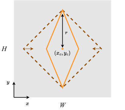
(a) Rhombus

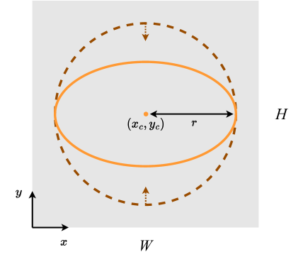
(b) Ellipse

Figure 3: The area enclosed by the dashed brown line is the preset deformation shape, and the area enclosed by the solid orange line is the actual deformation shape.

For the preset deformation shapes, we choose to define them using the $\ell_{1}$ and $\ell_{2}$ norm (rhombus and ellipse) in this work to facilitate calculation. Note that other shapes like a rectangle, which corresponds to the $\ell_{\infty}$ norm, could also work.

For the $\ell_{1}$ norm, the preset deformation shape $s$ is a rhombus, and the deformation region $S$ is defined as:

$$\{(x_{i},y_{i})\big{|}~{}~{}a_{x}\left|x_{i}-x_{c}\right|+a_{y}\left|y_{i}-y_{c}\right|<r\},$$ (1)

where $(x_{i},y_{i})$ is the coordinates of each pixel inside the deformation region.

For the $\ell_{2}$ norm, the preset deformation shape $s$ is an ellipse, and the deformation region $S$ is defined as:

$$\{(x_{i},y_{i})\big{|}~{}~{}a_{x}(x_{i}-x_{c})^{2}+a_{y}(y_{i}-y_{c})^{2}<r^{2}\}.$$ (2)

For each pixel $(x_{i},y_{i})$ in $S$, LOMA calculates a new position of this pixel and moves it accordingly to obtain the output image $I^{+}$:

$$\left\{\begin{array}[]{lr}x_{o}=\frac{d}{r}\cdot(x_{i}-x_{c})+x_{c},\\ y_{o}=\frac{d}{r}\cdot(y_{i}-y_{c})+y_{c},\\ I^{+}[x_{i},y_{i}]\leftarrow I[x_{o},y_{o}]\\ \end{array}\right.$$ (3)

where $d=\sqrt{(x_{i}-x_{c})^{2}+(y_{i}-y_{c})^{2}}$ is the distance between the pixel to be changed and the magnification center. For each input image, $r$ is randomly set within a given range as $r=random(r_{min},r_{max}$) $\times\;max(H,W)$, and either $a_{x}$ or $a_{y}$ takes a random value within the given range $random(a_{min},a_{max})$ while the other is set to $1$. $r$ determines the scope of local magnification in the image, while $a_{x}$ and $a_{y}$ determine the intensity of the deformation within the preset deformation region.

The overall process is shown in Algorithm 1. We denote this method as LOMA_I and also refer to it as LOMA for brevity.

Input: input image $I$, image size $(W,H)$, probability $p$, preset deformation shape $s$, horizontal/vertical compression ratio range $(a_{min},a_{max})$, radius range $(r_{min},r_{max})$

Output: augmented image $I^{+}$

1 $I^{+}\leftarrow I$

2 if $random(0,1)>p$ then

3       return $I^{+}$

4      

5else

6       $r\leftarrow random(r_{min},r_{max}$) $\times max(H,W)$

7      if  $random(0,1)>0.5$  then

8             $a_{x}\leftarrow random(a_{min},a_{max})$; $a_{y}\leftarrow 1$

9      else

10             $a_{x}\leftarrow 1$; $a_{y}\leftarrow random(a_{min},a_{max})$

11       end if

12      

13      if $s=$ ‘rhombus’ then

14             Calculate $S$ by Eq. (1)

15      else

16             Calculate $S$ by Eq. (2)

17       end if

18      for $(x_{i},y_{i})\in S$ do

19             $d\leftarrow\sqrt{(x_{i}-x_{c})^{2}+(y_{i}-y_{c})^{2}}$

20             Calculate $x_{o},y_{o},$ and $I^{+}[x_{i},y_{i}]$ by Eq. (3)

21       end for

22      return $I^{+}$

23      

24 end if

Algorithm 1 Local Magnification on Image

3.2 LOMA in the Feature Space

Unlike the above augmentation in the image space, that applies LOMA with probability $p$ to each image in the mini-batch, LOMA in the feature space augments each mini-batch with probability $p_{f}$ in an intermediate layer of the neural network. Since adapting the idea of LOMA to an intermediate layer is straightforward, we focus on how to extend the idea of random cropping into the feature space, which we call FeatureMap Offset (FO).

We decide with probability $p_{f}$ whether to use both LOMA on the Feature Map and FeatureMap Offset simultaneously for a mini-batch of feature maps that comes from the $l^{th}$ convolutional block of the network (a smaller $l$ is closer to the input). But note that the two methods can also be used separately. FeatureMap Offset does not change the size of the feature map but applies the translation operation of an affine transformation to move the feature map and fill the vacated entries with 0. Three possible scenarios are shown in Fig. 4, with the feature maps shifted to the lower left, right and upper right, respectively.

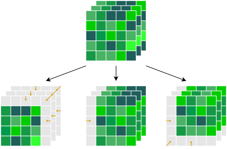
Figure 4: Examples of offsets in FeatureMap Offset (FO) method.

For each input feature map, the affine transformation matrix of FeatureMap Offset is:

$$M=\left[\begin{array}[]{ccc}1&0&T_{x}\\ 0&1&T_{y}\\ 0&0&1\\ \end{array}\right],$$ (4)

where $T_{x}$ and $T_{y}$ represent the offset of the feature map in the horizontal and vertical directions. Assuming the feature map size to be $B\times C\times H_{f}\times W_{f}$, then $T_{x}$ and $T_{y}$ each takes a random value in the given range $random(-\gamma,\gamma)\times max(H_{f},W_{f})$ , where $\gamma$ controls the offset degree of the feature map.

We abbreviate LOMA on the Feature Map as LOMA_F, abbreviate LOMA in the image space and feature space as LOMA_IF, and denote LOMA_IF together with FeatureMap Offset as LOMA_IF&FO.

4 Experiments

Method	CIFAR-10			CIFAR-100
	ResNet-20	WRN-28-10	PyramidNet	ResNet-20	WRN-28-10	PyramidNet
Baseline	92.75 $\pm$ 0.26	96.22 $\pm$ 0.10	96.16 $\pm$ 0.18	69.16 $\pm$ 0.28	81.32 $\pm$ 0.20	83.68 $\pm$ 0.34
Cutout [8]	93.67 $\pm$ 0.21	96.92 $\pm$ 0.16∗	96.90∗∗	70.16 $\pm$ 0.26	81.59 $\pm$ 0.27∗	83.47∗∗
Random Erasing [38]	93.27 $\pm$ 0.09∗	96.92 $\pm$ 0.05∗	-	70.03 $\pm$ 0.11∗	82.27 $\pm$ 0.15∗	-
LOMA (rhombus)	93.27 $\pm$ 0.10	96.85 $\pm$ 0.13	96.73 $\pm$ 0.32	70.12 $\pm$ 0.28	82.28 $\pm$ 0.23	83.91 $\pm$ 0.48
LOMA (ellipse)	93.26 $\pm$ 0.10	96.89 $\pm$ 0.11	96.79 $\pm$ 0.25	70.15 $\pm$ 0.19	81.88 $\pm$ 0.21	83.74 $\pm$ 0.19
LOMA_IF	93.42 $\pm$ 0.17	97.05 $\pm$ 0.12	96.74 $\pm$ 0.43	70.34 $\pm$ 0.36	82.65 $\pm$ 0.30	84.29 $\pm$ 0.58
LOMA_IF&FO	93.53 $\pm$ 0.15	96.97 $\pm$ 0.13	96.91 $\pm$ 0.60	70.57 $\pm$ 0.21	82.89 $\pm$ 0.23	84.45 $\pm$ 0.28

Table 1: Test accuracy (%) on CIFAR-10 and CIFAR-100. ^∗ indicates results reported in the original paper. ^∗∗ indicates results reported in another paper [34] for comparison. The best results are in bold and the second best results are underlined.

In this section, we verify the effectiveness of the proposed LOMA, LOMA_F and FO. We first conduct multiple experiments on the image classification task using the CIFAR-10, CIFAR-100 [19], and ImageNet [7] datasets (Sec. 4.1 and Sec. 4.2). Next, we study the impact of hyper-parameters on model performance and the robustness of the model to occlusion (Sec. 4.3 and Sec. 4.4). Then, we demonstrate the complementarity of LOMA to standard data augmentation (Sec. 4.5). Finally, we further evaluate our method on the PASCAL VOC 2007 detection benchmark [10] for object detection (Sec. 4.6).

4.1 Results on CIFAR-10 and CIFAR100

CIFAR-10 and CIFAR-100 [19] both have 60,000 color images of size 32$\times$32, and each dataset is divided into a training set of 50,000 images and a test set of 10,000 images. There are 10 and 100 different classes in CIFAR-10 and CIFAR-100, respectively. We train ResNet-20 [16] and WideResNet-28-10 [35] for 300 epochs using standard data augmentation (padding to 40$\times$40, random cropping, and random horizontal flipping) and Local Magnification (LOMA). And we utilize the Stochastic Gradient Descent (SGD) optimizer with Nesterov momentum of 0.9 and weight decay of 5e-4. The learning rate is set to 0.1 and decays by a factor of 10 at 100, 200, and 265 epochs. We also use PyramidNet-200 [14] with widening factor $\tilde{\alpha}=240$ in the same way as in Cutmix [34], where the batch size and training epochs are set to 64 and 300, respectively. The learning rate is set to 0.25 and decays 10-fold at 150 and 225 epochs. In the following experiments, we set $p=0.5$, $r_{max}=0.7$, $r_{min}=0.03$, $a_{max}=3$, $a_{min}=1$ for the hyper-parameters of LOMA, and $p_{f}=0.5$, $l=2$, $\gamma=0.25$ for the hyper-parameters of LOMA_F and FO, if not specified.

The results on CIFAR-10 and CIFAR-100 are summarized in Tab. 1. We see that LOMA (rhombus) and LOMA (eclipse) yield similar results. To avoid confusion, we only use LOMA (rhombus) for the following comparisons if not written explicitly. From the table, we can observe the following:

• When augmenting the image using LOMA at the input layer, our method improves the performance of the baseline significantly. The results of LOMA are competitive to, though do not surpass, two advanced intensity transformation data augmentation methods, Cutout [8] and Random Erasing [38].

• Using LOMA both in the image space and feature space, the resulting method LOMA_IF further boosts the performance, showing results similar to Cutout and Random Erasing on CIFAR-10 and outperforming them on CIFAR-100.

• Our final method LOMA_IF&FO outperforms Cutout and Random Erasing in almost all cases, except on CIFAR-10 using a ResNet-20 model. The superiority of LOMA_IF&FO is more prominent on more complex models and complicated data.

4.2 Results on ImageNet

The ILSVRC 2012 classification dataset [7], ImageNet, is the most challenging dataset for the image classification task. It contains about 1.2 million training images and 50,000 validation images with 1000 classes.

Method	ResNet-50
	Top-1 Err.	Top-5 Err.
Baseline	23.00	6.67
Cutout [8]	22.93∗∗	6.66∗∗
Random Erasing [38]	22.75∗	6.69∗
LOMA (rhombus)	22.63	6.69
LOMA (ellipse)	22.79	6.59
LOMA_IF	22.57	6.40
LOMA_IF&FO	22.33	6.30

Table 2: Test error (%) of ResNet-50 on the ImageNet dataset (the lower the better). ^∗ indicates results reported in the original paper. ^∗∗ indicates results reported in another paper [34] for comparison.

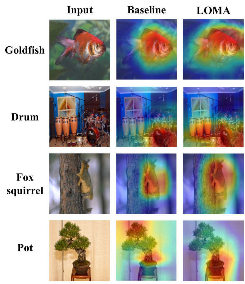
Figure 5: Class activation mapping (CAM) [39] visualizations for ResNet-50 trained on ImageNet. LOMA can force the network to focus on a larger range or more important region.

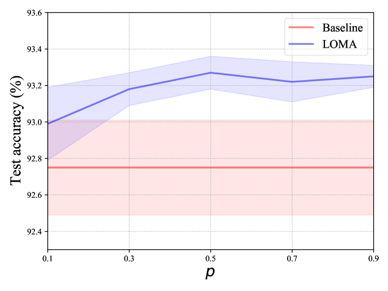
(a) Probability $p$

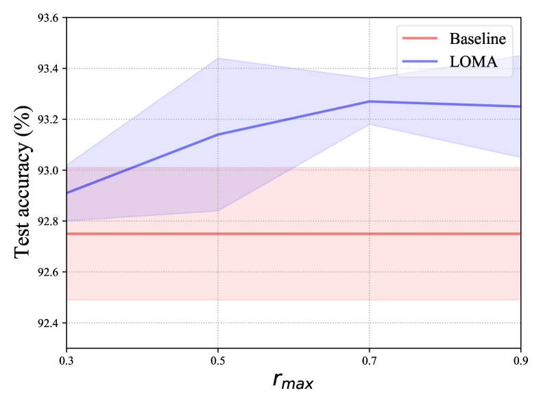
(b) Radius $r_{max}$

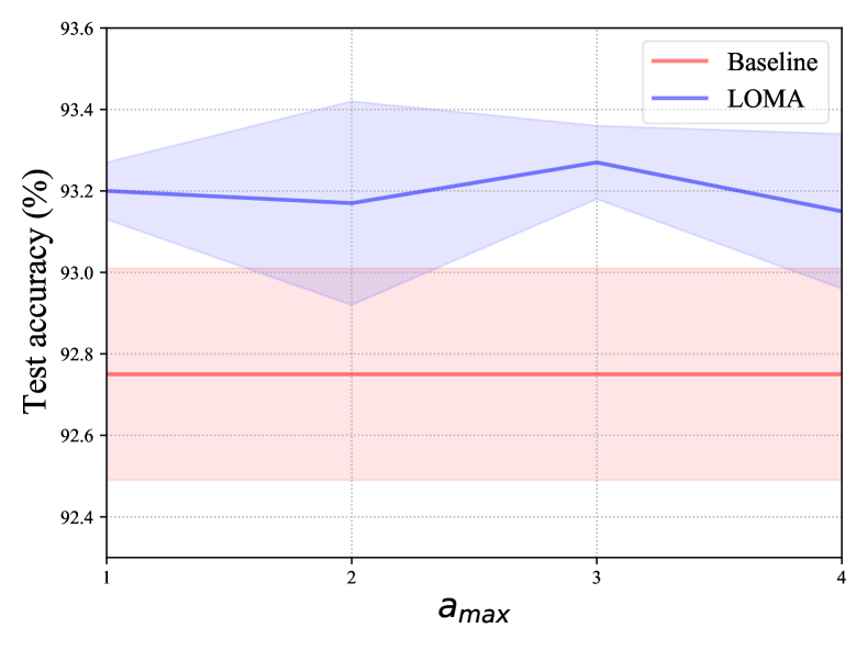
(c) Compression ratio $a_{max}$

Figure 6: Test accuracy (%) with different $p$, $r_{max}$, and $a_{max}$ on CIFAR-10 based on ResNet-20 using LOMA (rhombus).

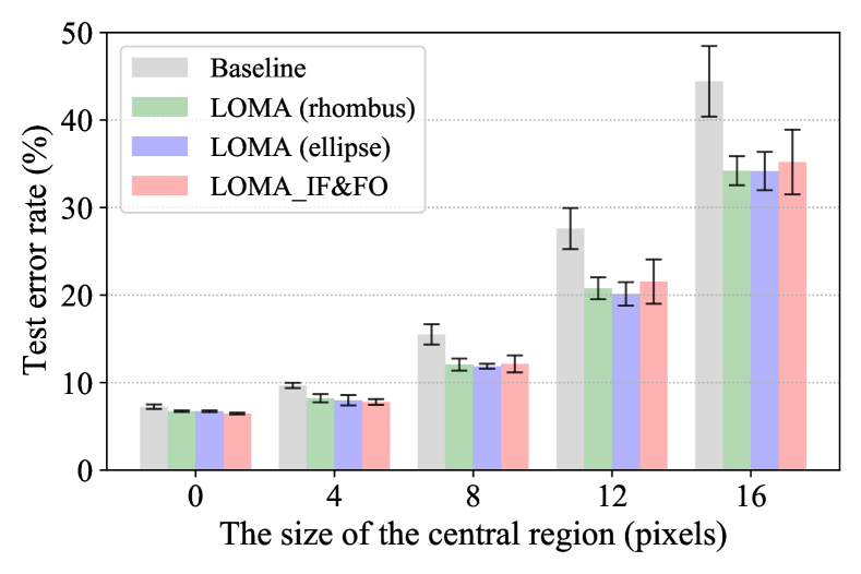
(a) Center occlusion

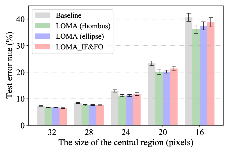
(b) Boundary occlusion

Figure 7: Robustness to occlusion on CIFAR-10 based on ResNet-20. A lower test error rate is better.

Following the training recipes in CutMix [34], we train ResNet-50 with LOMA and the standard data augmentations for 300 epochs using a weight decay of 1e-4. The batch size is set to 256. The learning rate starts from 0.1 and decays by a factor of 0.1 at epochs 75, 150 and 225, respectively. Since a more complicated dataset calls for an increased probability of augmentation, we set $p=0.8$ for ResNet-50.

The results on ImageNet are summarized in Tab. 2. To be consistent with the experiments on CIFAR datasets, if not specified, we continue to use LOMA (rhombus) for the comparison. From the results, we can observe the following:

	Baseline + LOMA	$l=1$	$l=2$	$l=3$
Top-1 Err.	17.72 $\pm$ 0.23	17.55 $\pm$ 0.12	17.11 $\pm$ 0.23	17.91 $\pm$ 0.58

Table 3: Test errors (%) of LOMA_F and FO applied to the $l$-th convolutional block of the network on CIFAR-100 based on WideResNet-28-10.

	Baseline + LOMA	$p_{f}=0.25$	$p_{f}=0.5$	$p_{f}=0.75$
Top-1 Err.	17.72 $\pm$ 0.23	17.32 $\pm$ 0.65	17.11 $\pm$ 0.23	17.37 $\pm$ 0.10

Table 4: Test errors (%) for different probability $p_{f}$ of LOMA_F and FO on CIFAR-100 based on WideResNet-28-10.

• When only augmenting the input images, LOMA (rhombus) and LOMA (ellipse) both boost the performance on the baseline (with standard data augmentation) and show similar or even better results over Cutout and Random Erasing.

• The results show continuous improvement after superimposing LOMA, LOMA_F, and FO sequentially on the baseline model (with standard data augmentation). LOMA_IF and LOMA_IF&FO both outperform the two advanced intensity transformation data augmentation methods, Cutout and Random Erasing.

Moreover, as shown in Fig. 5, LOMA can force the network to focus on a larger range or more important region than the baseline model, which will benefit the network performance. We believe that this occurs because the local magnification augmentations condition the network to model a significantly expanded appearance subspace for an object class without extending into the subspaces of other object classes.

4.3 Ablation Study

We explore the impact of hyper-parameters on LOMA, LOMA_F and FO in training the CNNs. In order to simplify the experiments, we conduct experiments on CIFAR-10 based on ResNet-20 using LOMA under different hyper-parameter settings, with the rhombus as the preset deformation shape. As a basic setting, we set $p=0.5$, $r_{max}=0.7$, $r_{min}=0.03$, $a_{max}=3$, and $a_{min}=1$ for LOMA. We experiment with different radius ranges, compression ratio ranges, and probabilities, and then examine their influence on the results. When modifying any one of them, the other two hyper-parameters are fixed. The results are summarized in Fig. 6.

Method	+LOMA_I	+LOMA_F	+FO	Accuracy (%)
Baseline				81.32 $\pm$ 0.20
	$\checkmark$			82.28 $\pm$ 0.23
		$\checkmark$		82.06 $\pm$ 0.10
			$\checkmark$	81.55 $\pm$ 0.41
	$\checkmark$	$\checkmark$		82.65 $\pm$ 0.30
		$\checkmark$	$\checkmark$	82.08 $\pm$ 0.27
	$\checkmark$	$\checkmark$	$\checkmark$	82.89 $\pm$ 0.23

Table 5: Test accuracy (%) of adding different components of our method to WideResNet-28-10 on CIFAR-100.

Method	+ RC	+ RF	+ LOMA	Accuracy (%)
Vanilla				89.35 $\pm$ 0.16
	$\checkmark$			94.29 $\pm$ 0.14
		$\checkmark$		92.50 $\pm$ 0.18
			$\checkmark$	90.66 $\pm$ 0.36
	$\checkmark$	$\checkmark$		95.32 $\pm$ 0.18
	$\checkmark$		$\checkmark$	94.99 $\pm$ 0.31
		$\checkmark$	$\checkmark$	93.60 $\pm$ 0.19
	$\checkmark$	$\checkmark$	$\checkmark$	95.82 $\pm$ 0.14

Table 6: Test accuracy (%) with different data augmentation on CIFAR-10 based on ResNet-18. RC: Random cropping, RF: Random flipping.

Method	train set	aero	bike	bird	boat	bottle	bus	car	cat	chair	cow	table	dog	horse	mbike	person	plant	sheep	sofa	train	tv	mAP
Faster RCNN	07	75.1	82.3	71.1	55.5	59.4	78.9	85.3	80.9	56.2	76.4	65.9	79.5	81.9	76.9	83.2	50.1	73.0	68.9	78.3	71.2	72.5
LOMA (rhombus)	07	82.0	81.9	73.2	59.4	59.4	79.6	85.2	80.6	59.0	70.1	63.3	78.8	80.9	81.3	83.4	50.5	68.8	71.4	80.0	73.1	73.2
LOMA (ellipse)	07	80.7	83.5	70.0	58.3	61.0	79.5	86.0	81.6	59.1	72.6	64.8	79.4	81.5	80.7	83.2	50.7	67.8	70.8	80.5	71.9	73.2
Faster RCNN	07+12	85.1	87.5	83.6	69.8	71.4	85.2	88.1	88.4	65.4	83.9	72.7	87.5	86.2	84.8	86.0	55.5	82.5	77.6	84.9	77.5	80.2
LOMA (rhombus)	07+12	84.6	86.7	83.8	69.0	70.8	84.9	88.1	88.6	65.5	84.9	73.1	87.9	85.4	85.6	85.8	58.7	83.6	79.0	85.1	81.0	80.6
LOMA (ellipse)	07+12	85.6	87.2	84.6	69.0	70.5	83.6	88.2	88.5	65.3	85.2	72.3	87.7	86.9	85.7	85.9	56.5	83.2	78.5	85.0	81.0	80.5

Table 7: Average precision (%) on VOC 2007 test set based on Faster RCNN.

It is important to note that no matter how the hyper-parameters are set, LOMA can always improve the model performance over the baseline. These experiments verify that different $r$ and $p$ can bring different effects to CNNs, as expected. Our method is also found to be robust to the compression ratios for the preset deformation shape.

For LOMA_F and FO, we explore the layer $l$ of feature argumentation to be applied, the probability $p$, and the necessity of having the two components. We experiment on CIFAR-100 based on WideResNet-28-10 using LOMA in the basic setting and LOMA_F and FO under different hyper-parameter settings.

As shown in Tabs. 3 and 4, applying LOMA_F and FO after the second convolution block works best. We believe this is because if it is too close to the input layer, the effect of moving the element position is very similar to that of LOMA in the input layer, thus bringing limited improvement. On the other hand, if it is too close to the output layer, it will affect the semantic information too much.

As shown in Tab. 5, we explore the contribution of individual components to the experimental results. The results show that all the three proposed methods can improve the classification accuracy separately, and data augmentation at the input layer is the most effective. The effect can be further improved when the three methods are combined, exceeding the baseline model by 1.67%.

4.4 Robustness to Occlusion

We study the robustness of the trained models with LOMA against occlusion on CIFAR-10 based on trained ResNet-20. We follow CutMix [34] to select regions of different sizes in the image’s central region and fill zeros in or outside the area to generate samples with different levels of occlusion.

Figure 7 illustrates the results. The models trained with LOMA or LOMA_IF&FO can significantly improve robustness compared to the baseline. Interestingly, in the model’s training process, the augmented image generated by LOMA does not directly block a specific part of the image. Thus, the model will not obtain any occluded samples, but when the level of blocking increases, whether by center occlusion or boundary occlusion, the effect of the model trained with our method is still better than that of the baseline. This proves that LOMA and LOMA_IF&FO can bring sufficient robustness against occlusion to the model.

4.5 Complementary to Standard Augmentation

We compare our method with random cropping and random flipping, two of the most commonly used and effective geometric transformation methods, and the results on ResNet-18 are shown in Tab. 6. Here “Vanilla” indicates training without any augmentation.

We notice that although our method does not perform as well as the standard augmentations when applied alone, it is complementary to them. When the three methods are used together, the error rate is 4.18%, outperforming the vanilla method by a large margin of 6.47%. Adding LOMA upon the current standard data augmentation (random cropping plus random flipping) further improves the accuracy by 0.5% on an already very high accuracy of 95.32%. The results indicate that the three methods of geometric transformation can be used together as a new standard data augmentation strategy for classification tasks.

4.6 Object Detection

The PASCAL VOC dataset [10] is a popular benchmark for object detection. The VOC 2007 dataset contains about 5,000 images over 20 object categories in the training/validation (trainval) set and 5,000 images in the test set. The VOC 2012 dataset contains about 11,000 images in the training/validation set. During the training, we use either the trainval in VOC 2007 or the union of VOC 2007 and VOC 2012 trainval as the training set. We evaluate our method’s performance on the VOC 2007 test set and use the mean average precision (mAP) metric. Faster RCNN [26] is employed as the detection model for these experiments, using the settings in the open source object detection toolbox MMDetection [2] based on PyTorch [24]. Since the backbone of the object detection task is already pre-trained, it is not suitable for further augmenting the feature map, so we only consider using LOMA here. For LOMA, we randomly select the location of the magnification center within the entire image and set $p=0.25$, $r_{max}=0.5$, and $a_{max}=1$.

The results are summarized in Tab. 7. When using VOC 2007 trainval for training, our method can achieve 0.7% improvements compared to the baseline, without needing to learn any extra parameters. When using the union of VOC 2007 and VOC 2012 trainval as the training set, the mAP of the detector trained with LOMA surpasses the baseline of Faster RCNN by 0.4%. The experiments show that our proposed method also benefits object detection tasks.

5 Conclusion

Different from global geometric transformation and occlusion methods, our model-free and easy-to-implement augmentation, Local Magnification (LOMA), randomly magnifies a part of the input image to generate more effective data for improving the model’s generalization. It can also complement global geometric transformation methods as a new standard data augmentation suite for training CNNs on both image classification and object detection tasks. The extension of LOMA and random cropping to feature augmentation can further boost the classification performance, and outperform the existing advanced data argumentation techniques based on intensity transformation. Our work shows two possible augmentation directions for model generalization: one is how to do distortion locally to strengthen the performance, the other is how to adapt effective data augmentation methods to feature augmentation. We will continue to investigate the two directions in our future work.

References

- [1] Antreas Antoniou, Amos Storkey, and Harrison Edwards. Data Augmentation Generative Adversarial Networks. arXiv preprint arXiv:1711.04340, 2017.
- [2] Kai Chen, Jiaqi Wang, Jiangmiao Pang, Yuhang Cao, Yu Xiong, Xiaoxiao Li, Shuyang Sun, Wansen Feng, Ziwei Liu, Jiarui Xu, Zheng Zhang, Dazhi Cheng, Chenchen Zhu, Tianheng Cheng, Qijie Zhao, Buyu Li, Xin Lu, Rui Zhu, Yue Wu, Jifeng Dai, Jingdong Wang, Jianping Shi, Wanli Ouyang, Chen Change Loy, and Dahua Lin. MMDetection: Open MMLab Detection Toolbox and Benchmark. arXiv preprint arXiv:1906.07155, 2019.
- [3] Liang-Chieh Chen, George Papandreou, Iasonas Kokkinos, Kevin Murphy, and Alan L. Yuille. Deeplab: Semantic Image Segmentation with Deep Convolutional Nets, Atrous Convolution, and Fully Connected CRFs. IEEE Transactions on Pattern Analysis and Machine Intelligence, 40(4):834–848, 2017.
- [4] Pengguang Chen, Shu Liu, Hengshuang Zhao, and Jiaya Jia. Gridmask Data Augmentation. arXiv preprint arXiv:2001.04086, 2020.
- [5] Ekin D. Cubuk, Barret Zoph, Dandelion Mané, Vijay Vasudevan, and Quoc V. Le. AutoAugment: Learning Augmentation Strategies From Data. In IEEE Conference on Computer Vision and Pattern Recognition, CVPR, pages 113–123, 2019.
- [6] Ekin Dogus Cubuk, Barret Zoph, Jon Shlens, and Quoc Le. RandAugment: Practical Automated Data Augmentation with a Reduced Search Space. In Advances in Neural Information Processing Systems 33: Annual Conference on Neural Information Processing Systems 2020, NeurIPS, pages 702–703, 2020.
- [7] Jia Deng, Wei Dong, Richard Socher, Li-Jia Li, Kai Li, and Li Fei-Fei. ImageNet: A Large-Scale Hierarchical Image Database. In IEEE Conference on Computer Vision and Pattern Recognition, CVPR, pages 248–255, 2009.
- [8] Terrance DeVries and Graham W Taylor. Improved Regularization of Convolutional Neural Networks with Cutout. arXiv preprint arXiv:1708.04552, 2017.
- [9] Alexey Dosovitskiy, Lucas Beyer, Alexander Kolesnikov, Dirk Weissenborn, Xiaohua Zhai, Thomas Unterthiner, Mostafa Dehghani, Matthias Minderer, Georg Heigold, Sylvain Gelly, Jakob Uszkoreit, and Neil Houlsby. An Image is Worth 16x16 Words: Transformers for Image Recognition at Scale. In 9th International Conference on Learning Representations, ICLR, 2021.
- [10] Mark Everingham, Luc Van Gool, Christopher KI Williams, John Winn, and Andrew Zisserman. The Pascal Visual Object Classes (VOC) Challenge. International Journal of Computer Vision, 88(2):303–338, 2010.
- [11] Mojtaba Faramarzi, Mohammad Amini, Akilesh Badrinaaraayanan, Vikas Verma, and Sarath Chandar. Patchup: A Regularization Technique for Convolutional Neural Networks. arXiv preprint arXiv:2006.07794, 2020.
- [12] Golnaz Ghiasi, Tsung-Yi Lin, and Quoc V Le. Dropblock: A Regularization Method for Convolutional Networks. In Advances in Neural Information Processing Systems 31: Annual Conference on Neural Information Processing Systems 2018, NeurIPS, pages 10750–10760, 2018.
- [13] Ross B. Girshick. Fast R-CNN. In IEEE International Conference on Computer Vision, ICCV, pages 1440–1448, 2015.
- [14] Dongyoon Han, Jiwhan Kim, and Junmo Kim. Deep Pyramidal Residual Networks. In IEEE Conference on Computer Vision and Pattern Recognition, CVPR, pages 5927–5935, 2017.
- [15] Ryuichiro Hataya, Jan Zdenek, Kazuki Yoshizoe, and Hideki Nakayama. Faster Autoaugment: Learning Augmentation Strategies Using Backpropagation. In Proceedings of the European Conference on Computer Vision, ECCV, pages 1–16, 2020.
- [16] Kaiming He, Xiangyu Zhang, Shaoqing Ren, and Jian Sun. Deep Residual Learning for Image Recognition. In IEEE Conference on Computer Vision and Pattern Recognition, CVPR, pages 770–778, 2016.
- [17] Sheng-Wei Huang, Che-Tsung Lin, Shu-Ping Chen, Yen-Yi Wu, Po-Hao Hsu, and Shang-Hong Lai. AugGAN: Cross Domain Adaptation with GAN-based Data Augmentation. In Proceedings of the European Conference on Computer Vision, ECCV, pages 718–731, 2018.
- [18] Jang-Hyun Kim, Wonho Choo, and Hyun Oh Song. Puzzle Mix: Exploiting Saliency and Local Statistics for Optimal Mixup. In Proceedings of the 37th International Conference on Machine Learning, ICML, pages 5275–5285, 2020.
- [19] Alex Krizhevsky, Geoffrey Hinton, et al. Learning Multiple Layers of Features from Tiny Images. Technical report, 2009.
- [20] Alex Krizhevsky, Ilya Sutskever, and Geoffrey E. Hinton. ImageNet Classification with Deep Convolutional Neural Networks. In Advances in Neural Information Processing Systems 25: Annual Conference on Neural Information Processing Systems 2012, NeurIPS, pages 1106–1114, 2012.
- [21] Boyi Li, Felix Wu, Ser-Nam Lim, Serge Belongie, and Kilian Q Weinberger. On Feature Normalization and Data Augmentation. In IEEE Conference on Computer Vision and Pattern Recognition, CVPR, pages 12383–12392, 2021.
- [22] Sungbin Lim, Ildoo Kim, Taesup Kim, Chiheon Kim, and Sungwoong Kim. Fast AutoAugment. In Advances in Neural Information Processing Systems 32: Annual Conference on Neural Information Processing Systems 2019, NeurIPS, pages 6662–6672, 2019.
- [23] Jonathan Long, Evan Shelhamer, and Trevor Darrell. Fully Convolutional Networks for Semantic Segmentation. In IEEE Conference on Computer Vision and Pattern Recognition, CVPR, pages 3431–3440, 2015.
- [24] Adam Paszke, Sam Gross, Soumith Chintala, Gregory Chanan, Edward Yang, Zachary DeVito, Zeming Lin, Alban Desmaison, Luca Antiga, and Adam Lerer. Automatic Differentiation in Pytorch. 2017.
- [25] Joseph Redmon, Santosh Kumar Divvala, Ross B. Girshick, and Ali Farhadi. You Only Look Once: Unified, Real-Time Object Detection. In IEEE Conference on Computer Vision and Pattern Recognition, CVPR, pages 779–788, 2016.
- [26] Shaoqing Ren, Kaiming He, Ross Girshick, and Jian Sun. Faster R-CNN: Towards Real-time Object Detection with Region Proposal Networks. In Advances in Neural Information Processing Systems 28: Annual Conference on Neural Information Processing Systems 2015, NeurIPS, pages 91–99, 2015.
- [27] Patrice Y Simard, David Steinkraus, John C Platt, et al. Best Practices for Convolutional Neural Networks Applied to Visual Document Analysis. In 7th International Conference on Document Analysis and Recognition, ICDAR, pages 958–963, 2003.
- [28] Karen Simonyan and Andrew Zisserman. Very Deep Convolutional Networks for Large-Scale Image Recognition. In 3rd International Conference on Learning Representations, ICLR, 2015.
- [29] Krishna Kumar Singh and Yong Jae Lee. Hide-and-seek: Forcing a Network to Be Meticulous for Weakly-Supervised Object and Action Localization. In IEEE International Conference on Computer Vision, ICCV, pages 3524–3533, 2017.
- [30] Nitish Srivastava, Geoffrey Hinton, Alex Krizhevsky, Ilya Sutskever, and Ruslan Salakhutdinov. Dropout: A Simple Way to Prevent Neural Networks from Overfitting. The journal of machine learning research, 15(1):1929–1958, 2014.
- [31] Teppei Suzuki. TeachAugment: Data Augmentation Optimization Using Teacher Knowledge. In IEEE Conference on Computer Vision and Pattern Recognition, CVPR, pages 10904–10914, 2022.
- [32] Haohang Xu, Shuangrui Ding, Xiaopeng Zhang, Hongkai Xiong, and Qi Tian. Masked Autoencoders are Robust Data Augmentors. arXiv preprint arXiv:2206.04846, 2022.
- [33] Mingle Xu, Sook Yoon, Alvaro Fuentes, and Dong Sun Park. A Comprehensive Survey of Image Augmentation Techniques for Deep Learning. arXiv preprint arXiv:2205.01491, 2022.
- [34] Sangdoo Yun, Dongyoon Han, Sanghyuk Chun, Seong Joon Oh, Youngjoon Yoo, and Junsuk Choe. CutMix: Regularization Strategy to Train Strong Classifiers With Localizable Features. In IEEE International Conference on Computer Vision, ICCV, pages 6022–6031, 2019.
- [35] Sergey Zagoruyko and Nikos Komodakis. Wide Residual Networks. In Proceedings of the British Machine Vision Conference, BMVC, 2016.
- [36] Hongyi Zhang, Moustapha Cissé, Yann N. Dauphin, and David Lopez-Paz. Mixup: Beyond Empirical Risk Minimization. In 6th International Conference on Learning Representations, ICLR, 2018.
- [37] Xinyu Zhang, Qiang Wang, Jian Zhang, and Zhao Zhong. Adversarial AutoAugment. In 8th International Conference on Learning Representations, ICLR, 2020.
- [38] Zhun Zhong, Liang Zheng, Guoliang Kang, Shaozi Li, and Yi Yang. Random Erasing Data Augmentation. In The Thirty-Fourth AAAI Conference on Artificial Intelligence, AAAI, pages 13001–13008, 2020.
- [39] Bolei Zhou, Aditya Khosla, Agata Lapedriza, Aude Oliva, and Antonio Torralba. Learning Deep Features for Discriminative Localization. In IEEE Conference on Computer Vision and Pattern Recognition, CVPR, pages 2921–2929, 2016.