Abstract

New $Q$-conditional (nonclassical) symmetries and exact solutions of the hunter-gatherer–farmer population model proposed by Aoki, Shida and Shigesada (Theor Popul Biol 1996;50:1–17) are constructed. The main method used for the aforementioned purposes is an extension of the nonclassical method for system of partial differential equations. An analysis of properties of the exact solutions obtained and their biological interpretation are carried out. New results are compared with those derived in recent studies devoted to the same model.

Keywords: reaction-diffusion system; population dynamics; exact solution;
conditional symmetry; nonclassical symmetry.

1 Introduction

In this work, we study the model, which was suggested in [2] for modeling competition between farmers and hunter-gatherers that took place thousands of years ago. Nowadays this model is extensively studied by different mathematical techniques [1, 33, 20, 21]. In particular, a detailed archeological background of the model is presented in [1]. The model reflects the recent DNA studies, which have shown that early farming spread through most of Europe by the range expansion of farmers of Anatolian origin took place simultaneously with by the conversion to farming of the European hunter-gatherers, and have confirmed that these hunter-gatherers continued to coexist with the incoming farmers. It means that three essentially different populations, native farmers from Anatolia, converted farmers with origins in Europe and hunter-gatherers, coexisted for many years (see [1] and references cited therein).

This work is a natural continuation of our recent studies [12, 14], in which Lie and $Q$-conditional (nonclassical) symmetries of this model were identified and exact solutions were constructed. Moreover a biological interpretation of the solutions obtained was provided as well. First of all, we remind the reader that after relevant re-scaling (see [12] for details), the model in the 1D approximation takes the form of the nonlinear reaction-diffusion (RD) system

$$\begin{array}[]{l}u_{t}=d_{1}u_{xx}+u(1-u-a_{1}v),\\ v_{t}=d_{2}v_{xx}+a_{2}v(1-u-a_{1}v)+uw+a_{1}vw,\\ w_{t}=d_{3}w_{xx}+a_{3}w(1-w)-a_{4}uw-a_{5}vw,\end{array}$$ (1)

where $u(t,x),\ v(t,x)$ and $w(t,x)$ are nondimensional densities of populations of initial farmers, converted farmers, and hunter-gatherers, respectively (hereinafter the lower subscripts $t$ and $x$ mean differentiation w.r.t. these variables). System (1) is called the hunter-gatherer–farmer (HGF) model and is the main object of investigation in this paper. We naturally assume that the diffusivities $d_{1},\ d_{2}$ and $d_{3}$ are positive constants. Other parameters are nonnegative constant, moreover $a_{1}>0$ (otherwise system (1) has an autonomous equation and this means that the other two populations have no impact on the initial farmer population) and $a_{4}>0$ (otherwise the carrying capacity of farmers is zero [2]). Thus, we consider the HGF system (1) with the restrictions

$$d_{1}>0,d_{2}>0,d_{3}>0,a_{1}>0,a_{2}\geq 0,a_{3}\geq 0,a_{4}>0,a_{5}\geq 0.$$ (2)

The main aims of this paper are to derive new nonclassical symmetries and exact solutions of the HGF system (1), analyse the properties of the solutions obtained and propose their biological interpretation. The main method we are using here is an extension of the nonclassical method for partial differential equations (PDEs). The latter was firstly suggested by Bluman and Cole [8] and was further developed in many papers (see reviews [31, 30] and monographs [18, 11] for recent citations). The algorithm for finding $Q$-conditional symmetries (following [22], we use this terminology instead of nonclassical symmetries) of a given PDE is based on the classical Lie method. However, in contrast to the case of Lie symmetry, the corresponding system of determining equations is nonlinear and its general solution can be found only in exceptional cases. If one deals with a system of PDEs then the problem becomes much more complicated. As a result, almost all works devoted to the construction of $Q$-conditional symmetries were published within the last 10–15 years [9, 3, 32, 5, 13, 14, 11]. To the best of our knowledge, there are only a few papers devoted to nonclassical symmetries of PDE systems published in the early 2000s [4, 17, 28].

Recently [14], $Q$-conditional symmetries and exact solutions were constructed for the HGF system (1) for the first time. However, a so-called ‘no-go case’ was not examined therein. Here we aim to examine this special case as well and to identify new $Q$-conditional symmetries. Moreover, it is shown that these $Q$-conditional symmetries lead to new exact solutions and some of them possess attractive properties, reflecting competition between farmers and hunter-gatherers.

The remainder of this paper is organized as follows. In Section 2, we introduce a modification of the notion of the $Q$-conditional symmetry of the first type, which is needed for the no-go case, and formulate the main theorem. In Section 3, the symmetry operators obtained in Section 2 are used to construct exact solutions of the HGF system (1). Analysis of the solutions derived in order to provide a biological interpretation is carried out as well. Finally, we briefly discuss the results obtained and compare them with those derived in other papers.

2 Main theoretical results

First of all, we formulate the main definition used for deriving new $Q$-conditional symmetries of the HGF system (1). Consider an evolution system of $m$ second-order equations with two independent $(t,x)$ and $m$ dependent $u=(u^{1},u^{2},\dots,u^{m})$ variables

$$u_{t}^{i}=F^{i}\left(t,x,u,u_{x},u_{xx}\right),\ i=1,2,\dots,m,\ m\geq 2.$$ (3)

Here $F^{i}$ are smooth functions of the corresponding variables, the subscripts $t$ and $x$ denote differentiation w.r.t. these variables, $u_{t}^{i}\equiv\frac{\partial u^{i}}{\partial t}$, $u_{x}\equiv\frac{\partial u}{\partial x}=\left(\frac{\partial u^{1}}{\partial x},\dots,\frac{\partial u^{m}}{\partial x}\right),$ and $u_{xx}\equiv\frac{\partial^{2}u}{\partial x^{2}}=\left(\frac{\partial^{2}u^{1}}{\partial x^{2}},\dots,\frac{\partial^{2}u^{m}}{\partial x^{2}}\right)$.

Let us consider the general form of a $Q$-conditional symmetry of system (3) :

$$Q=\xi^{0}(t,x,u)\partial_{t}+\xi^{1}(t,x,u)\partial_{x}+\eta^{1}(t,x,u)\partial_{u^{1}}+\ldots+\eta^{m}(t,x,u)\partial_{u^{m}},$$ (4)

where $\xi^{i}(t,x,u)$ and $\eta^{k}(t,x,u)$ are smooth functions to-be-determined using the well-known criterion (see, e.g., [7, Chapter 5]). For the formulation of the criterion, the notion of the second prolongation of the operator $Q$ is needed. We remind the reader that the first prolongation is

$$\mbox{\raisebox{-7.3194pt}{$\stackrel{{\scriptstyle\displaystyle Q}}{{\scriptstyle 1}}$}}=Q+\rho^{1}_{t}\partial_{u^{1}_{t}}+\ldots+\rho^{m}_{t}\partial_{u^{m}_{t}}+\rho^{1}_{x}\partial_{u^{1}_{x}}+\ldots+\rho^{m}_{x}\partial_{u^{m}_{x}},$$

hence the second prolongation can be written as

$$\mbox{\raisebox{-7.3194pt}{$\stackrel{{\scriptstyle\displaystyle Q}}{{\scriptstyle 2}}$}}=\mbox{\raisebox{-7.3194pt}{$\stackrel{{\scriptstyle\displaystyle Q}}{{\scriptstyle 1}}$}}+\sigma^{1}_{tt}\partial_{u^{1}_{tt}}+\ldots+\sigma^{m}_{tt}\partial_{u^{m}_{tt}}+\sigma^{1}_{tx}\partial_{u^{1}_{tx}}+\ldots+\sigma^{m}_{tx}\partial_{u^{m}_{tx}}+\sigma^{1}_{xx}\partial_{u^{1}_{xx}}+\ldots+\sigma^{m}_{xx}\partial_{u^{m}_{xx}},$$

where the coefficients $\rho$ and $\sigma$ with relevant subscripts are expressed via the functions $\xi^{0},\ \xi^{1}$ and $\eta^{k}$ and their derivatives by the well- known formulae (see, e.g., [7, 11]). Actually, the formulae of prolongations of infinitesimal operators were constructed by Sophus Lie in his classical works in the 1880s [26, 27].

Definition 1

Operator (4) is called a $Q$-conditional symmetry (nonclassical symmetry) for an evolution system of the form (3) if the invariance criterion is satisfied:

$$\mbox{\raisebox{-6.88889pt}{$\stackrel{{\scriptstyle\displaystyle Q}}{{\scriptstyle 2}}$}}\,(S_{i})\Big{|}_{{\cal{M}}}=0,\ i=1,2,\ldots,m.$$ (5)

Here $\stackrel{{\scriptstyle\displaystyle Q}}{{\scriptstyle 2}}$ is the second prolongation of the operator $Q$ and the manifold

$${\cal{M}}=\left\{S_{i}=0,Q\left(u^{i}\right)=0,\frac{\partial}{\partial t}\,Q\left(u^{i}\right)=0,\frac{\partial}{\partial x}\,Q\left(u^{i}\right)=0,i=1,\dots,m\right\},$$

where

$$S_{i}\equiv u_{t}^{i}-F^{i}\left(t,x,u,u_{x},u_{xx}\right),\ Q\left(u^{i}\right)\equiv\xi^{0}{u^{i}}_{t}+\xi^{1}{u^{i}}_{x}-\eta^{i}.$$

Remark 1

In the case of a Lie symmetry operator, the manifold

$${\cal{M}}_{0}=\left\{S_{i}=0,i=1,\dots,m\right\}\supset{\cal{M}}$$

should be applied instead of the Manifold ${\cal{M}}$.

Remark 2

It is shown in [11, Section 2.3] that the differential consequences $\frac{\partial}{\partial t}\,Q\left(u^{i}\right)=0$ and $\frac{\partial}{\partial x}\,Q\left(u^{i}\right)=0$ can be ignored when $\xi^{0}\neq 0$ and the system in question is one of the evolution type.

It is well-known that solving the problem of constructing $Q$-conditional symmetries of evolution systems depends essentially on the function $\xi^{0}$ because one should consider two different cases :

1. $\xi^{0}\neq 0;$

2. $\xi^{0}=0,\ \xi^{1}\neq 0.$

Here we examine only Case 2, for which the terminology ‘no-go case’ is often used. Indeed, Case 1 for the HGF system (1) was investigated in [14]. First of all, we note that the task of constructing $Q$-conditional symmetries with $\xi^{0}=0$ for scalar evolution equations is reducible to solving the equation in question [34]. This statement can be extended on system of evolution equations. In other words, it means that application of the invariance criteria (5) to operator (4) with $\xi^{0}=0$ after cumbersome calculations leads to a system of determining equations, which is reducible to (3). So, in the case of nonlinear and nonintegrable equations (systems), one can identify only some particular $Q$-conditional symmetries of the form (4) with $\xi^{0}=0$. Notably, even the particular cases obtained by applying Definition 1 may lead to new exact solutions and/or can be useful for developing new techniques such as the algorithm of heir equations [29, 23].

A new algorithm was suggested in [9], which allow us to construct special subsets of $Q$-conditional symmetries in a simpler way. The algorithm is based on the notion of the $Q$-conditional symmetry of the $p$-th type ($p=1,\dots,m$). In the case $p=m,$ this notion leads exactly to the notion of the standard $Q$-conditional (nonclassical) symmetry. In the case $p=1$, $Q$-conditional symmetries of the first type are obtained, which form a special subset of the set of $Q$-conditional symmetries. It should be stressed that the no-go case was ignored in [9]. Recently [13], we have shown that the definition of the $Q$-conditional symmetry proposed in [9] should be modified in the no-go case. Having done this, the above mentioned algorithm allowed us to derive new $Q$-conditional symmetries for the diffusive Lotka–Volterra (DLV) system. Now we generalize Definition 2 [13] on any evolution system.

Definition 2

Operator

$$Q=\xi(t,x,u)\partial_{x}+\eta^{1}(t,x,u)\partial_{u^{1}}+\ldots+\eta^{m}(t,x,u)\partial_{u^{m}},\ \xi\neq 0,$$ (6)

is called a $Q$-conditional symmetry of the first type for an evolution system of the form (3) if the following invariance criterion is satisfied:

$$\mbox{\raisebox{-6.88889pt}{$\stackrel{{\scriptstyle\displaystyle Q}}{{\scriptstyle 2}}$}}\,(S_{i})\Big{|}_{{\cal{M}}^{j}_{1}}=0,\ i=1,2,\ldots,m,$$

where the Manifold ${\cal{M}}^{j}_{1}$ with a fixed number $\ j\ (1\leq j\leq m)$ is

$$\left\{S_{1}=0,S_{2}=0,\dots,S_{m}=0,Q\left(u^{j}\right)=0,\frac{\partial}{\partial t}\,Q\left(u^{j}\right)=0,\frac{\partial}{\partial x}\,Q\left(u^{j}\right)=0\right\}.$$

In the case of evolution system (3), the algorithm of a complete classification of $Q$-conditional symmetries of the first type consists of $m$ steps. The first step reduces to the application of Definition 2 in the case

$${\cal{M}}^{1}_{1}=\left\{S_{1}=0,\dots,S_{m}=0,Q\left(u^{1}\right)=0,\frac{\partial}{\partial t}\,Q\left(u^{1}\right)=0,\frac{\partial}{\partial x}\,Q\left(u^{1}\right)=0\right\}$$

and solving a relevant system of determining equations. The next $m-1$ steps are quite similar and one should deal with the manifolds ${\cal{M}}^{2}_{1},\dots,{\cal{M}}^{m}_{1}$ instead of ${\cal{M}}^{1}_{1}$. If the system in question possesses a symmetric structure the number of steps can be reduced. The typical example is the two-component DLV system, for which a single step is enough (see [13] for details). However, if a given system does not possess a symmetric structure and does not involve a subsystem with such structure then the algorithm consists of $m$ steps.

Now we turn back to the HGF system (1). In this case, operator (6) has the form

$$\begin{array}[]{l}Q=\xi(t,x,u,v,w)\partial_{x}+\eta^{1}(t,x,u,v,w)\partial_{u}\vskip 6.0pt plus 2.0pt minus 2.0pt\\ +\eta^{2}(t,x,u,v,w)\partial_{v}+\eta^{3}(t,x,u,v,w)\partial_{w}.\end{array}$$ (7)

Our aim is to find all possible $Q$-conditional symmetries of the first type (7) for the HGF system (1).

Remark 3

In Theorem 1, the upper indices $u$ and $w$ mean that the relevant $Q$-conditional symmetry operators satisfy Definition 2 in the case of the Manifold ${\cal{M}}^{1}_{1}$ ($u^{1}=u$) and ${\cal{M}}^{3}_{1}$ ($u^{3}=w$), respectively.

Theorem 1

The HGF system (1) with restrictions (2) is invariant under a $Q$-conditional symmetry (symmetries) of the first type (7) if and only if the system and the corresponding symmetry operator(s) have the forms listed below.

Case I. $d_{1}\neq d_{2}$ :

$$\textbf{Subcase I.a}\hskip 14.22636pt\begin{array}[]{l}u_{t}=d_{1}u_{xx}+u(1-u-a_{1}v),\\ v_{t}=d_{2}v_{xx}+v(1-u-a_{1}v)+uw+a_{1}vw,\\ w_{t}=d_{3}w_{xx}+a_{3}w(1-w)-a_{4}w(u+a_{1}v),\ a_{3}\neq 0,\end{array}$$ (8)

$$Q^{u}_{1}=a_{1}\partial_{x}+\frac{\alpha_{1}+2\alpha_{2}x}{\alpha_{0}+\alpha_{1}x+\alpha_{2}x^{2}+2d_{1}\alpha_{2}t}\,u\left(a_{1}\partial_{u}-\partial_{v}\right);$$

$$\textbf{Subcase I.b}\hskip 14.22636pt\begin{array}[]{l}u_{t}=d_{1}u_{xx}+u(1-u-a_{1}v),\\ v_{t}=d_{2}v_{xx}+v(1-u-a_{1}v)+uw+a_{1}vw,\\ w_{t}=d_{3}w_{xx}-a_{4}w(u+a_{1}v),\end{array}$$ (9)

$$Q^{u}_{1},\ Q^{w}_{2}=\partial_{x}+e^{t}(\alpha_{0}+\alpha_{1}x)\,w^{\frac{1}{a_{4}}}\left(a_{1}\partial_{u}-\partial_{v}\right);$$

$$\textbf{Subcase I.c}\hskip 14.22636pt\begin{array}[]{l}u_{t}=d_{1}u_{xx}+u(1-u-a_{1}v),\\ v_{t}=d_{2}v_{xx}+a_{2}v(1-u-a_{1}v)+uw+a_{1}vw,\\ w_{t}=d_{3}w_{xx}-uw-a_{1}vw,\end{array}$$ (10)

$$Q^{u}_{3}=a_{1}\partial_{x}+f_{1}(t,x)\,u\left(a_{1}\partial_{u}-\partial_{v}+(1-a_{2})\partial_{w}\right),$$

$$Q^{w}_{3}=(1-a_{2})\partial_{x}+f_{3}(t,x)\,w\left(a_{1}\partial_{u}-\partial_{v}+(1-a_{2})\partial_{w}\right),$$

where $a_{2}=\frac{d_{2}-d_{3}}{d_{1}-d_{3}}$, $\kappa=\frac{1}{\sqrt{\mid d_{1}-d_{3}\mid}},$

$$f_{i}(t,x)=\left\{\begin{array}[]{l}\frac{\kappa\left(\alpha_{1}\cos(\kappa\,x)-\alpha_{2}\sin(\kappa\,x)\right)}{\alpha_{0}\exp(d_{i}\kappa^{2}t)+\alpha_{1}\sin(\kappa\,x)+\alpha_{2}\cos(\kappa\,x)},\ \mbox{if}\ d_{1}>d_{3},\vskip 6.0pt plus 2.0pt minus 2.0pt\\ \frac{\kappa\left(\alpha_{1}e^{\kappa x}-\alpha_{2}e^{-\kappa x}\right)}{\alpha_{0}\exp(-d_{i}\kappa^{2}t)+\alpha_{1}e^{\kappa x}+\alpha_{2}e^{-\kappa x}},\ \mbox{if}\ d_{1}<d_{3},\end{array}\right.i=1,3;$$

Case II. $d_{1}=d_{2}=1$ :

$$\textbf{Subcase II.a}\hskip 14.22636pt\begin{array}[]{l}u_{t}=u_{xx}+u(1-u-a_{1}v),\\ v_{t}=v_{xx}+v(1-u-a_{1}v)+uw+a_{1}vw,\\ w_{t}=d_{3}w_{xx}+a_{3}w(1-w)-a_{4}w(u+a_{1}v),\ a_{3}\neq 0,\end{array}$$ (11)

$$Q^{u}_{4}=\partial_{x}+g(t,x)\,u\left(a_{1}\partial_{u}-\partial_{v}\right),$$

where $g(t,x)$ is an arbitrary solution of the Burgers equation $g_{t}=g_{xx}+2a_{1}gg_{x}$;

$$\textbf{Subcase II.b}\hskip 14.22636pt\begin{array}[]{l}u_{t}=u_{xx}+u(1-u-a_{1}v),\\ v_{t}=v_{xx}+v(1-u-a_{1}v)+uw+a_{1}vw,\\ w_{t}=d_{3}w_{xx}-a_{4}w(u+a_{1}v),\ a_{4}\neq 1,\end{array}$$ (12)

$$Q^{u}_{4},\ Q^{w}_{5}=\partial_{x}+e^{t}\Big{(}\alpha_{1}(1-u-a_{1}v)+\alpha_{2}e^{-t}u+\frac{\alpha_{1}a_{1}}{1-a_{4}}w+h(t,x)w^{\frac{1}{a_{4}}}\Big{)}\left(a_{1}\partial_{u}-\partial_{v}\right);$$

$$\textbf{Subcase II.c}\hskip 14.22636pt\begin{array}[]{l}u_{t}=u_{xx}+u(1-u-a_{1}v),\\ v_{t}=v_{xx}+v(1-u-a_{1}v)+uw+a_{1}vw,\\ w_{t}=d_{3}w_{xx}-uw-a_{1}vw,\end{array}$$ (13)

$$Q^{u}_{4},\ Q^{w}_{6}=\partial_{x}+e^{t}\Big{(}\alpha_{1}(1-u-a_{1}v)+\alpha_{2}e^{-t}u-\alpha_{1}a_{1}w\ln w+h(t,x)w\Big{)}\left(a_{1}\partial_{u}-\partial_{v}\right).$$

Here $\alpha$ with subscripts are arbitrary constants, while the function $h(t,x)$ is an arbitrary solution of the linear heat equation $h_{t}=h_{xx}.$

Remark 4

The functions $f_{1}$ and $f_{3}$ reduce to some constants (see the operators $Q^{u}_{3}$ and $Q^{w}_{3}$ with $d_{1}<d_{3}$) by setting $\alpha_{0}=\alpha_{1}=0$ or $\alpha_{0}=\alpha_{2}=0$.

Sketch of the proof. In order to derive a complete classification of $Q$-conditional symmetries of the first type, we should apply the algorithm described above. Since system (1) does not possess the symmetric structure the algorithm consist of three steps. This means that we should consider the following three manifolds

$${\cal{M}}_{1}^{1}=\left\{S_{1}=0,S_{2}=0,S_{3}=0,Q(u)=0,\frac{\partial}{\partial t}\,Q(u)=0,\frac{\partial}{\partial x}\,Q(u)=0\right\},$$

$${\cal{M}}_{1}^{2}=\left\{S_{1}=0,S_{2}=0,S_{3}=0,Q(v)=0,\frac{\partial}{\partial t}\,Q(v)=0,\frac{\partial}{\partial x}\,Q(v)=0\right\}$$

and

$${\cal{M}}_{1}^{3}=\left\{S_{1}=0,S_{2}=0,S_{3}=0,Q(w)=0,\frac{\partial}{\partial t}\,Q(w)=0,\frac{\partial}{\partial x}\,Q(w)=0\right\},$$

and separately apply Definition 2 for each manifold. Thus, three different systems of determining equations should be derived and further solved.

Let us use the notations

$$\begin{array}[]{l}G^{1}=u(1-u-a_{1}v),\\ G^{2}=a_{2}v(1-u-a_{1}v)+uw+a_{1}vw,\\ G^{3}=a_{3}w(1-w)-a_{4}uw-a_{5}vw\end{array}$$ (14)

in order to avoid cumbersome formulae. So, system (1) takes the form

$$\begin{array}[]{l}u_{t}=d_{1}u_{xx}+G^{1}(u,v,w),\\ v_{t}=d_{2}v_{xx}+G^{2}(u,v,w),\\ w_{t}=d_{3}w_{xx}+G^{3}(u,v,w).\end{array}$$ (15)

Applying Definition 2 with the Manifold ${\cal{M}}_{1}^{1}$ to the RD system (15) and making straightforward calculations (see a similar routine in Section 3.3 [18]), we arrive at the following system of determining equations :

$$\xi_{v}=\xi_{w}=\eta^{1}_{vv}=\eta^{1}_{ww}=\eta^{1}_{vw}=\eta^{2}_{vv}=\eta^{2}_{ww}=\eta^{2}_{vw}\vskip 6.0pt plus 2.0pt minus 2.0pt$$

$$\hskip 56.9055pt=\eta^{3}_{vv}=\eta^{3}_{ww}=\eta^{3}_{vw}=0,\vskip 6.0pt plus 2.0pt minus 2.0pt$$ (16)

$$(d_{1}-d_{2})\eta^{1}_{v}=0,\ (d_{1}-d_{3})\eta^{1}_{w}=0,\ (d_{2}-d_{3})\eta^{2}_{w}=0,\ (d_{2}-d_{3})\eta^{3}_{v}=0,\vskip 6.0pt plus 2.0pt minus 2.0pt$$ (17)

$$\xi\eta^{1}_{xv}+\eta^{1}\eta^{1}_{uv}=0,\ \xi\eta^{1}_{xw}+\eta^{1}\eta^{1}_{uw}=0,\ \eta^{1}\xi_{u}+\xi\xi_{x}=0,\vskip 6.0pt plus 2.0pt minus 2.0pt$$ (18)

$$(d_{1}-d_{2})\eta^{1}_{w}\eta^{2}_{u}=2d_{2}(\xi\eta^{2}_{xw}+\eta^{1}\eta^{2}_{uw}),(d_{1}-d_{3})\eta^{1}_{v}\eta^{3}_{u}=2d_{3}(\xi\eta^{3}_{xv}+\eta^{1}\eta^{3}_{uv}),\hskip 14.22636pt\vskip 6.0pt plus 2.0pt minus 2.0pt$$ (19)

$$2d_{2}\eta^{2}_{xv}+G^{1}\xi_{u}+\xi_{t}+\frac{1}{\xi}\Big{(}d_{1}\xi_{u}\eta^{1}_{x}+2d_{2}\eta^{1}\eta^{2}_{uv}\Big{)}+d_{1}\frac{\eta^{1}}{\xi^{2}}\,\xi_{u}\eta^{1}_{u}=0,\vskip 6.0pt plus 2.0pt minus 2.0pt$$ (20)

$$2d_{3}\eta^{3}_{xw}+G^{1}\xi_{u}+\xi_{t}+\frac{1}{\xi}\Big{(}d_{1}\xi_{u}\eta^{1}_{x}+2d_{3}\eta^{1}\eta^{3}_{uw}\Big{)}+d_{1}\frac{\eta^{1}}{\xi^{2}}\,\xi_{u}\eta^{1}_{u}=0,\vskip 6.0pt plus 2.0pt minus 2.0pt$$ (21)

$$d_{1}\eta^{1}_{xx}-\eta^{1}_{t}-G^{1}\eta^{1}_{u}-G^{2}\eta^{1}_{v}-G^{3}\eta^{1}_{w}+G^{1}_{u}\eta^{1}+G^{1}_{v}\eta^{2}+G^{1}_{w}\eta^{3}\vskip 6.0pt plus 2.0pt minus 2.0pt$$

$$+\frac{\eta^{1}}{\xi}\Big{(}2d_{1}\eta^{1}_{xu}+\xi_{t}+G^{1}\xi_{u}\Big{)}+d_{1}\frac{\eta^{1}}{\xi^{2}}\left(\eta^{1}\eta^{1}_{uu}+\xi_{u}\eta^{1}_{x}\right)+d_{1}\frac{{\eta^{1}}^{2}}{\xi^{3}}\,\xi_{u}\eta^{1}_{u}=0,\vskip 6.0pt plus 2.0pt minus 2.0pt$$ (22)

$$d_{2}\eta^{2}_{xx}-\eta^{2}_{t}-G^{1}\eta^{2}_{u}-G^{2}\eta^{2}_{v}-G^{3}\eta^{2}_{w}+G^{2}_{u}\eta^{1}+G^{2}_{v}\eta^{2}+G^{2}_{w}\eta^{3}\vskip 6.0pt plus 2.0pt minus 2.0pt$$

$$+\frac{1}{\xi}\Big{(}2d_{2}\eta^{1}\eta^{2}_{xu}+(d_{2}-d_{1})\eta^{1}_{x}\eta^{2}_{u}\Big{)}+\frac{\eta^{1}}{\xi^{2}}\Big{(}d_{2}\eta^{1}\eta^{2}_{uu}+(d_{2}-d_{1})\eta^{1}_{u}\eta^{2}_{u}\Big{)}=0,\vskip 6.0pt plus 2.0pt minus 2.0pt$$ (23)

$$d_{3}\eta^{3}_{xx}-\eta^{3}_{t}-G^{1}\eta^{3}_{u}-G^{2}\eta^{3}_{v}-G^{3}\eta^{3}_{w}+G^{3}_{u}\eta^{1}+G^{3}_{v}\eta^{2}+G^{3}_{w}\eta^{3}\vskip 6.0pt plus 2.0pt minus 2.0pt$$

$$+\frac{1}{\xi}\Big{(}2d_{3}\eta^{1}\eta^{3}_{xu}+(d_{3}-d_{1})\eta^{1}_{x}\eta^{3}_{u}\Big{)}+\frac{\eta^{1}}{\xi^{2}}\Big{(}d_{3}\eta^{1}\eta^{3}_{uu}+(d_{3}-d_{1})\eta^{1}_{u}\eta^{3}_{u}\Big{)}=0.$$ (24)

Now we present a detailed analysis of system (16)–(24). First of all, we note that equations (17) lead to five essentially different cases, namely:
(i) $\eta^{1}_{v}=\eta^{1}_{w}=\eta^{2}_{w}=\eta^{3}_{v}=0$ and all diffusivities $d_{1},\ d_{2}$ and $d_{3}$ are arbitrary constants;
(ii) $\eta^{1}_{v}\neq 0\Rightarrow d_{1}=d_{2}$, $\eta^{1}_{w}=\eta^{2}_{w}=\eta^{3}_{v}=0$ and $d_{3}$ is an arbitrary constant;
(iii) $\eta^{1}_{w}\neq 0\Rightarrow d_{1}=d_{3}$, $\eta^{1}_{v}=\eta^{2}_{w}=\eta^{3}_{v}=0$ and $d_{2}$ is an arbitrary constant;
(iv) $\left(\eta^{2}_{w}\right)^{2}+\left(\eta^{3}_{v}\right)^{2}\neq 0\Rightarrow d_{2}=d_{3}$, $\eta^{1}_{v}=\eta^{1}_{w}=0$ and $d_{1}$ is an arbitrary constant;
(v) $\eta^{1}_{v}\eta^{1}_{w}=0,\ \left(\eta^{1}_{v}\right)^{2}+\left(\eta^{1}_{w}\right)^{2}\neq 0$ and $\left(\eta^{2}_{w}\right)^{2}+\left(\eta^{3}_{v}\right)^{2}\neq 0\Rightarrow d_{1}=d_{2}=d_{3};$
(vi) $\eta^{1}_{v}\eta^{1}_{w}\not=0\Rightarrow$ $d_{1}=d_{2}=d_{3}.$

Consider case (i). Integrating the linear equations (16), we calculate that the functions $\xi,\ \eta^{1},\ \eta^{2}$ and $\eta^{3}$ have the form

$$\begin{array}[]{l}\xi=\xi(t,x,u),\ \eta^{1}=r^{1}(t,x,u),\ \eta^{2}=r^{2}(t,x,u)+q^{2}(t,x,u)\,v,\\ \eta^{3}=r^{3}(t,x,u)+q^{3}(t,x,u)\,w,\end{array}$$ (25)

where $\xi,\ r^{i},\ q^{2}$ and $q^{3}$ are to-be-determined functions. Taking into account formulae (25), we note that equations (19) vanish, while those from (18) reduce to the single equation $\eta^{1}\xi_{u}+\xi\xi_{x}=0$.

Now one can substitute (14) and (25) into equations (20)–(24). Since the unknown functions $\xi,\ r^{1},\ r^{2},\ r^{3},\ q^{2}$ and $q^{3}$ do not depend on $v$ and $w$, we can split the equations obtained w.r.t. these variables and their products. In particular, equation (20) takes the form

$$2d_{2}q^{2}_{x}+u(1-u-a_{1}v)\xi_{u}+\xi_{t}+\frac{1}{\xi}\Big{(}d_{1}\xi_{u}r^{1}_{x}+2d_{2}r^{1}q^{2}_{u}\Big{)}+d_{1}\frac{r^{1}}{\xi^{2}}\,\xi_{u}r^{1}_{u}=0.$$

Splitting the last equation w.r.t. the variable $v$, one immediately obtains $\xi_{u}=0$ (see restrictions (2)), therefore $\xi=\xi(t)$. So, equation (20) simplifies to the form

$$\xi_{t}+2d_{2}q^{2}_{x}+\frac{2d_{2}}{\xi}r^{1}q^{2}_{u}=0.$$ (26)

Similarly, splitting equation (23) w.r.t. $vw$ one gets: $q^{3}=0\Rightarrow\xi=const$ (see equation (21)), i.e. we can set $\xi=1$ without losing a generality. Thus, formulae (25) take the forms

$$\xi=1,\ \eta^{1}=r^{1}(t,x,u),\ \eta^{2}=r^{2}(t,x,u)+q^{2}(t,x,u)\,v,\ \eta^{3}=r^{3}(t,x,u).$$ (27)

In other words, the functions (27) form the general solution of the subsystem of determining equations consisting of (16)–(21) with $r^{1}$ and $q^{2}$ satisfying (26). In order to solve the remaining equations (22)–(24), we substitute (14) and (27) into these equations and split the expressions obtained w.r.t. $v$ and its powers. As a result, we arrive at

$$a_{5}q^{2}=0,\ -a_{4}r^{1}-a_{5}r^{2}-2a_{3}r^{3}=0,\ uq^{2}-r^{1}-a_{1}r^{2}=0,\vskip 6.0pt plus 2.0pt minus 2.0pt$$ (28)

$$ur^{1}_{u}-r^{1}-uq^{2}=0,a_{1}ur^{3}_{u}-a_{5}r^{3}=0,uq^{2}_{u}-a_{2}q^{2}=0,r^{1}q^{2}_{u}+q^{2}_{x}=0,\hskip 11.38092pt\vskip 6.0pt plus 2.0pt minus 2.0pt$$ (29)

$$d_{1}r^{1}_{xx}-r^{1}_{t}+d_{1}\left(r^{1}\right)^{2}r^{1}_{uu}+2d_{1}r^{1}r^{1}_{xu}\vskip 6.0pt plus 2.0pt minus 2.0pt$$

$$\hskip 28.45274pt+u(u-1)r^{1}_{u}+(1-2u)r^{1}-a_{1}ur^{2}=0,\vskip 6.0pt plus 2.0pt minus 2.0pt$$ (30)

$$d_{2}r^{2}_{xx}-r^{2}_{t}+d_{2}\left(r^{1}\right)^{2}r^{2}_{uu}+2d_{2}r^{1}r^{2}_{xu}+a_{2}(1-u)r^{2}+ur^{3}\vskip 6.0pt plus 2.0pt minus 2.0pt$$

$$\hskip 28.45274pt+\big{(}u(u-1)+(d_{2}-d_{1})r^{1}r^{1}_{u}+(d_{2}-d_{1})r^{1}_{x}\big{)}r^{2}_{u}=0,\vskip 6.0pt plus 2.0pt minus 2.0pt$$ (31)

$$d_{3}r^{3}_{xx}-r^{3}_{t}+d_{3}\left(r^{1}\right)^{2}r^{3}_{uu}+2d_{3}r^{1}r^{3}_{xu}+(a_{3}-a_{4}u)r^{3}\vskip 6.0pt plus 2.0pt minus 2.0pt$$

$$\hskip 28.45274pt+\big{(}u(u-1)+(d_{3}-d_{1})r^{1}r^{1}_{u}+(d_{3}-d_{1})r^{1}_{x}\big{)}r^{3}_{u}=0,\vskip 6.0pt plus 2.0pt minus 2.0pt$$ (32)

$$d_{2}q^{2}_{xx}-q^{2}_{t}+d_{2}\left(r^{1}\right)^{2}q^{2}_{uu}+2d_{2}r^{1}q^{2}_{xu}+a_{1}ur^{2}_{u}-a_{2}r^{1}-2a_{1}a_{2}r^{2}+a_{1}r^{3}\vskip 6.0pt plus 2.0pt minus 2.0pt$$

$$\hskip 28.45274pt+\big{(}u(u-1)+(d_{2}-d_{1})r^{1}r^{1}_{u}+(d_{2}-d_{1})r^{1}_{x}\big{)}q^{2}_{u}=0.$$ (33)

Equations (28) are algebraic constraints on functions from (27). Analyzing the first equation from (28), we need to consider two subcases : (i1) $a_{5}\neq 0;$ (i2) $a_{5}=0$.

In subcase (i1), we obtain $q^{2}=0$. Integrating the first two equations from (29) and using the last equation from (28), we arrive at the functions $r^{1},\ r^{2}$ and $r^{3}$:

$$r^{1}=f^{1}(t,x)\,u,\ r^{2}=-\frac{f^{1}(t,x)}{a_{1}}\,u,\ r^{3}=f^{2}(t,x)\,u^{\frac{a_{5}}{a_{1}}},$$ (34)

where $f^{1}$ and $f^{2}$ are to-be-determined smooth functions.

Substituting $q^{2}=0$ and (34) into system (28)–(33), we obtain the system

$$(a_{1}a_{4}-a_{5})f^{2}=0,\ (a_{1}a_{4}-a_{5})f^{1}\,u+2a_{1}a_{3}f^{2}\,u^{\frac{a_{5}}{a_{1}}}=0,\vskip 6.0pt plus 2.0pt minus 2.0pt$$ (35)

$$(a_{2}-1)f^{1}\,u+a_{1}f^{2}\,u^{\frac{a_{5}}{a_{1}}}=0,\vskip 6.0pt plus 2.0pt minus 2.0pt$$ (36)

$$f^{1}_{t}=d_{1}f^{1}_{xx}+2d_{1}f^{1}f^{1}_{x},\vskip 6.0pt plus 2.0pt minus 2.0pt$$ (37)

$$f^{1}_{t}=d_{2}f^{1}_{xx}+(3d_{2}-d_{1})f^{1}f^{1}_{x}+(d_{2}-d_{1})\left(f^{1}\right)^{3}+(a_{2}-1)f^{1},\vskip 6.0pt plus 2.0pt minus 2.0pt$$ (38)

$$a_{1}f^{2}_{t}=a_{1}d_{3}f^{2}_{xx}+2a_{5}d_{3}f^{1}f^{2}_{x}+a_{5}(d_{3}-d_{1})f^{2}f^{1}_{x}\vskip 6.0pt plus 2.0pt minus 2.0pt$$

$$+\frac{a_{5}(a_{5}d_{3}-a_{1}d_{1})}{a_{1}}\left(f^{1}\right)^{2}f^{2}+(a_{1}a_{3}-a_{5})f^{2},\qquad$$ (39)

which involves three algebraic equations. Assuming $f^{2}\neq 0$, it is easily shown that equations (35)–(36) produce

$$f^{2}=\frac{1-a_{2}}{a_{1}}\,f^{1},\ a_{3}=0,\ a_{4}=1,\ a_{5}=a_{1}.$$

Now we realize that system (37)–(39) is an overdetermined nonlinear system of PDEs on the function $f^{1}$. Note that the restriction $d_{1}\neq d_{2}$ should hold (otherwise the contradiction $(a_{2}-1)f^{1}=0$ is obtained, see equations (37)–(38)). It can be shown by straightforward calculations that system (37)–(39) has nonzero solutions if and only if the restriction $a_{2}=\frac{d_{2}-d_{3}}{d_{1}-d_{3}}\not=1$ holds.

Equations (38) and (39) coincide under the above restriction. Excluding the derivative $f^{1}_{t}$ from equation (37) and substituting into (38) we arrive exactly at the equation

$$f^{1}_{xx}+3f^{1}f^{1}_{x}+\left(f^{1}\right)^{3}+\frac{1}{d_{1}-d_{3}}\,f^{1}=0.$$ (40)

It is well-known (see, e.g., [25]) that the nonlinear equation (40) is reducible to the linear third-order ordinary differential equation (ODE)

$$(d_{1}-d_{3})g_{xxx}+g_{x}=0,$$ (41)

by the nonlocal substitution $f^{1}=\frac{g_{x}}{g}$, where $g(t,x)$ is a new unknown function. Integrating the linear equation (41), we derive two types of its general solutions depending on the sign of $d_{1}-d_{3}.$ Substituting each of them into equation (37), we obtain two forms of the function $f_{1}$ listed in Theorem 1. Thus, we arrive at the operator $Q^{u}_{3}$ of the HGF system (10).

Now we assume that $f^{2}=0$ and $f^{1}\neq 0$ (for $f^{1}=0$ the Lie symmetry operator $\partial_{x}$ is obtained) and immediately arrive at the restrictions $a_{5}=a_{1}a_{4},\ a_{2}=1.$ In this case, system (37)–(39) is reducible to

$$\begin{array}[]{l}f^{1}_{t}=d_{1}f^{1}_{xx}+2d_{1}f^{1}f^{1}_{x},\vskip 6.0pt plus 2.0pt minus 2.0pt\\ (d_{1}-d_{2})\left(f^{1}_{xx}+3f^{1}f^{1}_{x}+\left(f^{1}\right)^{3}\right)=0.\end{array}$$ (42)

Now one realizes that the above system has the same structure as that integrated above. Solving system (42) and taking into account (27) and (34), we obtain operator $Q^{u}_{1}$ of the HGF system (8) (in the case $d_{1}\neq d_{2}$) and operator $Q^{u}_{4}$ of system (11) (in the case $d_{1}=d_{2}$). Thus, case (i) is completely investigated and the operators $Q^{u}_{1},\ Q^{u}_{3}$ and $Q^{u}_{4}$ are constructed.

Cases (ii)–(vi) were also studied. It was proved that new $Q$-conditional symmetry operators are not obtainable.

Applying Definition 2 in the case of the Manifold ${\cal{M}}^{3}_{1}$ in a quite similar way, the operators $Q^{w}_{2},\ Q^{w}_{3},\ Q^{w}_{5}$ and $Q^{w}_{6}$ were identified for systems (9), (10), (12) and (13), respectively.

Finally, it was checked by applying Definition 2 in the case of the Manifold ${\cal{M}}^{2}_{1}$ that the HGF system (1) does not admit new $Q$-conditional symmetry operators.

The sketch of the proof is now completed. $\square$

Remark 5

The system of determining equations (16)–(24) is valid for any RD system of the form (15).

Now we present the following observation. All the HGF systems presented in Case I of Theorem 1 admit only a trivial Lie symmetry generated by the operators of time and space translations (see, Theorem 2.1 [12]). All the HGF systems listed in Case II of Theorem 1 admit nontrivial Lie symmetries, which can be directly obtained from the relevant $Q$-conditional symmetries. Indeed, the HGF systems (11), (12) and (13) admit the Lie symmetry operator $\partial_{x}+\alpha u(a_{1}\partial_{u}-\partial_{v})$ (see Case 4 of Table 1 [12]) that follows from the operator $Q^{u}_{4}$ if one sets $g(t,x)=\alpha$. As follows from Case 9 of Table 1 [12], the HGF systems (12) and (13) with $d_{3}=1$ additionally admit the Lie symmetry operators $\partial_{x}+\alpha e^{t}\Big{(}1-u-a_{1}v+\frac{a_{1}}{1-a_{4}}w\Big{)}\left(a_{1}\partial_{u}-\partial_{v}\right)$ ($a_{4}\not=1$) and $\partial_{x}+\alpha e^{t}w\left(a_{1}\partial_{u}-\partial_{v}\right)$ ($a_{4}=1$), respectively. These Lie symmetry operators can be easily obtained as particular cases from the operators $Q^{w}_{5}$ and $Q^{w}_{6}$, respectively. This observation is in agreement with the conditional symmetry theory, which says that Lie symmetries should follow from conditional symmetries as particular cases.

In conclusion of this section, we present a new result about conditional symmetries of the DLV systems. It can be checked that the systems arising in Case II of Theorem 1 are reducible to the DLV systems by the transformation

$$u\rightarrow u,\ u+a_{1}v\rightarrow v,\ w\rightarrow w.$$ (43)

In fact, applying transformation (43) to system (11) and the operator $Q_{4}^{u}$, we obtain the DLV system

$$\begin{array}[]{l}u_{t}=u_{xx}+u(1-v),\\ v_{t}=v_{xx}+v(1-v+a_{1}w),\\ w_{t}=d_{3}w_{xx}+w(a_{3}-a_{4}v-a_{3}w),\end{array}$$ (44)

and the operator

$${Q^{u}_{4}}^{*}=\partial_{x}+g(t,x)\,u\partial_{u},$$ (45)

where the function $g$ is again an arbitrary solution of the Burgers equation $g_{t}=g_{xx}+2gg_{x}.$ In the case $a_{3}=0,$ the DLV system (44) additionally admits the $Q$-conditional symmetry operator

$${Q^{w}_{5}}^{*}=\partial_{x}+e^{t}\Big{(}\alpha_{1}(1-v)+\alpha_{2}e^{-t}u+\frac{\alpha_{1}a_{1}}{1-a_{4}}w+h(t,x)w^{\frac{1}{a_{4}}}\Big{)}\,\partial_{u},$$ (46)

if $a_{4}\neq 1$, and

$${Q^{w}_{6}}^{*}=\partial_{x}+e^{t}\Big{(}\alpha_{1}(1-v)+\alpha_{2}e^{-t}u-\alpha_{1}a_{1}w\ln w+h(t,x)w\Big{)}\,\partial_{u},$$ (47)

if $a_{4}=1.$

It should be pointed out that operators (45)–(47) have different structures from those constructed in [10]. So, we have derived examples of new $Q$-conditional (nonclassical) symmetries of the DLV system (44).

3 Exact solutions and their interpretation

In this section, our aim is to construct new exact solutions of the HGF system using the conditional symmetries obtained above and to suggest their possible biological interpretations. In what follows, we restrict ourselves to two systems, (10) and (11). The first one was examined because the corresponding symmetries have the most complicated structure. In fact, only operators $Q^{u}_{3}$ and $Q^{w}_{3}$ involve $\eta^{1}\neq 0,\ \eta^{2}\neq 0$ and $\eta^{3}\neq 0$ (see $\eta^{i}$ in (7)), while $\eta^{3}=0$ in all other conditional symmetries.The HGF system (11) was examined because one has identical structure (up to notations) to the system investigated recently in [20] and [21]. It should be stressed that all other $Q$-conditional symmetry operators listed in Theorem 1 can be applied to search for exact solutions in the same way.

3.1 The HGF system (10)

Let us construct exact solutions of the HGF system (10) using the operators $Q^{u}_{3}$ and $Q^{w}_{3}$. Firstly we note that one can set $a_{1}=1$ without losing a generality because of the transformation $u\rightarrow u,\ a_{1}v\rightarrow v,\ a_{1}w\rightarrow w$, hence system (10) and its operators take the forms

$$\begin{array}[]{l}u_{t}=d_{1}u_{xx}+u(1-u-v),\\ v_{t}=d_{2}v_{xx}+\frac{d_{2}-d_{3}}{d_{1}-d_{3}}\,v(1-u-v)+uw+vw,\\ w_{t}=d_{3}w_{xx}-uw-vw,\end{array}$$ (48)

$$\begin{array}[]{l}Q^{u}_{3}=\partial_{x}+f_{1}(t,x)\,u\left(\partial_{u}-\partial_{v}+(1-a_{2})\partial_{w}\right),\\ \vskip 6.0pt plus 2.0pt minus 2.0ptQ^{w}_{3}=(1-a_{2})\partial_{x}+f_{3}(t,x)\,w\left(\partial_{u}-\partial_{v}+(1-a_{2})\partial_{w}\right),\ a_{2}=\frac{d_{2}-d_{3}}{d_{1}-d_{3}}.\end{array}$$

In order to construct the ansatz generated by the operator $Q^{u}_{3}$, according to the standard procedure one needs to use a so-called invariance surface condition. In this case, it is the first-order PDE system

$$\begin{array}[]{l}u_{x}=f_{1}(t,x)\,u,\ v_{x}=-f_{1}(t,x)\,u,\ w_{x}=\frac{d_{1}-d_{2}}{d_{1}-d_{3}}f_{1}(t,x)\,u,\end{array}$$ (49)

where $f_{1}$ is defined in Theorem 1.

Depending on the form of the function $f_{1}$, the integration of system (49) leads to the ansatz

$$\begin{array}[]{l}u(t,x)=\varphi_{1}(t)\Big{(}\alpha_{0}+\alpha_{1}\sin(\kappa\,x)\exp(-d_{1}\kappa^{2}t)+\alpha_{2}\cos(\kappa\,x)\exp(-d_{1}\kappa^{2}t)\Big{)},\vskip 6.0pt plus 2.0pt minus 2.0pt\\ v(t,x)=\varphi_{2}(t)-u(t,x),\vskip 6.0pt plus 2.0pt minus 2.0pt\\ w(t,x)=\varphi_{3}(t)+\frac{d_{1}-d_{2}}{d_{1}-d_{3}}\,u(t,x),\end{array}$$ (50)

if $d_{1}>d_{3}$, and the ansatz

$$\begin{array}[]{l}u(t,x)=\varphi_{1}(t)\Big{(}\alpha_{0}+\alpha_{1}\exp(\kappa\,x+d_{1}\kappa^{2}t)+\alpha_{2}\exp(-\kappa\,x+d_{1}\kappa^{2}t)\Big{)},\vskip 6.0pt plus 2.0pt minus 2.0pt\\ v(t,x)=\varphi_{2}(t)-u(t,x),\vskip 6.0pt plus 2.0pt minus 2.0pt\\ w(t,x)=\varphi_{3}(t)+\frac{d_{1}-d_{2}}{d_{1}-d_{3}}\,u(t,x),\end{array}$$ (51)

if $d_{1}<d_{3}$. Here $\varphi_{1}(t),\ \varphi_{2}(t)$ and $\varphi_{3}(t)$ are new unknown functions, while $\kappa=\frac{1}{\sqrt{\mid d_{1}-d_{3}\mid}}.$

Substituting ansatz (50) into the HGF system (48), we arrive at the ODE system

$$\begin{array}[]{l}\varphi_{1}^{\prime}+\varphi_{1}(\varphi_{2}-1)=0,\vskip 6.0pt plus 2.0pt minus 2.0pt\\ \varphi_{2}^{\prime}-\varphi_{2}\varphi_{3}+\frac{d_{2}-d_{3}}{d_{1}-d_{3}}\,\varphi_{2}(\varphi_{2}-1)-\frac{\alpha_{0}(d_{1}-d_{2})}{d_{1}-d_{3}}\,\varphi_{1}=0,\vskip 6.0pt plus 2.0pt minus 2.0pt\\ \varphi_{3}^{\prime}+\varphi_{2}\varphi_{3}+\frac{\alpha_{0}(d_{1}-d_{2})}{d_{1}-d_{3}}\,\varphi_{1}=0.\end{array}$$ (52)

It turns out that ansatz (51) leads to the same ODE system.

The ODE system (52) is nonlinear and its complete integration is beyond the scope of this work. However, we were able to construct particular solutions of (52). It turns out that the solutions obtained lead to those of the HGF system (48), which possess highly attractive properties.

First of all, we note that the ODE system (52) possesses two steady-state points

$$(\varphi_{1},\varphi_{2},\varphi_{3})=(0,0,w_{0}),\quad(\varphi_{1},\varphi_{2},\varphi_{3})=\left(u_{0},1,\alpha_{0}u_{0}\frac{d_{2}-d_{1}}{d_{1}-d_{3}}\right),$$

where $u_{0}$ and $w_{0}$ are arbitrary parameters. The first steady-state point leads to a trivial solution of the the HGF system (48), however, the second one, after substituting into (50) and (51), produces new four-parameter families of exact solutions. Ansatz (50) produces the solutions of the form

$$\begin{array}[]{l}u(t,x)=u_{0}\Big{(}\alpha_{0}+\alpha_{1}\sin(\kappa\,x)\exp(-d_{1}\kappa^{2}t)+\alpha_{2}\cos(\kappa\,x)\exp(-d_{1}\kappa^{2}t)\Big{)},\vskip 6.0pt plus 2.0pt minus 2.0pt\\ v(t,x)=1-u_{0}\Big{(}\alpha_{0}+\alpha_{1}\sin(\kappa\,x)\exp(-d_{1}\kappa^{2}t)+\alpha_{2}\cos(\kappa\,x)\exp(-d_{1}\kappa^{2}t)\Big{)},\vskip 6.0pt plus 2.0pt minus 2.0pt\\ w(t,x)=u_{0}\frac{d_{1}-d_{2}}{d_{1}-d_{3}}\Big{(}\alpha_{1}\sin(\kappa\,x)\exp(-d_{1}\kappa^{2}t)+\alpha_{2}\cos(\kappa\,x)\exp(-d_{1}\kappa^{2}t)\Big{)},\end{array}$$ (53)

while ansatz (51) leads to those of the form

$$\begin{array}[]{l}u(t,x)=u_{0}\Big{(}\alpha_{0}+\alpha_{1}\exp(\kappa\,x+d_{1}\kappa^{2}t)+\alpha_{2}\exp(-\kappa\,x+d_{1}\kappa^{2}t)\Big{)},\vskip 6.0pt plus 2.0pt minus 2.0pt\\ v(t,x)=1-u_{0}\Big{(}\alpha_{0}+\alpha_{1}\exp(\kappa\,x+d_{1}\kappa^{2}t)+\alpha_{2}\exp(-\kappa\,x+d_{1}\kappa^{2}t)\Big{)},\vskip 6.0pt plus 2.0pt minus 2.0pt\\ w(t,x)=u_{0}\frac{d_{1}-d_{2}}{d_{1}-d_{3}}\Big{(}\alpha_{1}\exp(\kappa\,x+d_{1}\kappa^{2}t)+\alpha_{2}\exp(-\kappa\,x+d_{1}\kappa^{2}t)\Big{)},\end{array}$$

where $\alpha_{i}$ and $u_{0}$ are arbitrary parameters.

For example, let us consider a particular case $\alpha_{2}=0$ and assume that three populations of initial farmers, converted farmers, and hunter-gatherers are interacting in the domain

$$\Omega_{\kappa}=\left\{(t,x)\in(0,+\infty)\times\Big{(}\frac{2k\pi}{\kappa},\frac{(2k+1)\pi}{\kappa}\Big{)}\right\},\ k\in\mathbb{Z}.$$

Now we observe that the exact solution (53) takes the form

$$\begin{array}[]{l}u(t,x)=u_{0}\Big{(}\alpha_{0}+\alpha_{1}\sin(\kappa\,x)\exp(-d_{1}\kappa^{2}t))\Big{)},\vskip 6.0pt plus 2.0pt minus 2.0pt\\ v(t,x)=1-u_{0}\alpha_{0}-u_{0}\alpha_{1}\sin(\kappa\,x)\exp(-d_{1}\kappa^{2}t),\vskip 6.0pt plus 2.0pt minus 2.0pt\\ w(t,x)=u_{0}\alpha_{1}\frac{d_{1}-d_{2}}{d_{1}-d_{3}}\sin(\kappa\,x)\exp(-d_{1}\kappa^{2}t),\end{array}$$ (54)

and is nonnegative (the population densities cannot be negative) in $\Omega_{\kappa}$ provided

$$u_{0}(\alpha_{0}+\alpha_{1})\geq 0,\ 1\geq u_{0}(\alpha_{0}+\alpha_{1}),\ 1\geq u_{0}\alpha_{0},\ u_{0}\alpha_{1}(d_{1}-d_{2})\geq 0.$$

Moreover solution (54) possesses the asymptotical behavior

$$(u,\,v,\,w)\rightarrow\left(u_{0}\alpha_{0},\,1-u_{0}\alpha_{0},\,0\right)\ \texttt{as}\ t\rightarrow+\infty.$$ (55)

Thus, the exact solution (54) describes such a scenario of interaction between three populations, which leads to the coexistence of farmers and converted farmers and to the extinction of hunter-gatherers (see an example in Fig. 1). There are also two special cases. The first one, $u_{0}\alpha_{0}=1$, describes the scenario leading to a complete extinction of two populations and only the initial farmers will survive. The second case, $\alpha_{0}=0,\ u_{0}\not=0$, says that eventually all hunter-gatherers convert into farmers, while all the initial farmers die out.

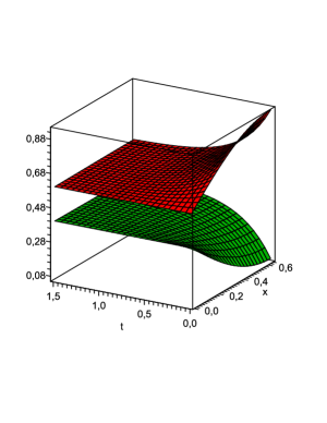
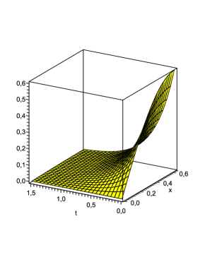
Figure 1: Surfaces representing the components $u$ (green), $v$ (red) and $w$ (yellow) of solution (54) with $u_{0}=1,\ \alpha_{0}=2/5,\ \alpha_{1}=-1/3,\ \kappa=\sqrt{6}$ of the HGF system (48) with the parameters $d_{1}=1/2,\ d_{2}=4/5,\ d_{3}=1/3$.

Now we present another approach for constructing exact solutions of the ODE system (52). Let us assume that $\varphi_{2}=\beta\varphi_{1},$ where $\beta\neq 0$ is an arbitrary constant. In this case, system (52) can be easily integrated and has the general solution

$$\begin{array}[]{l}\varphi_{1}=\frac{Ce^{t}}{1+\beta C(e^{t}-1)},\vskip 6.0pt plus 2.0pt minus 2.0pt\\ \varphi_{2}=\frac{\beta Ce^{t}}{1+\beta C(e^{t}-1)},\vskip 6.0pt plus 2.0pt minus 2.0pt\\ \varphi_{3}=\frac{(d_{1}-d_{2})\left(\beta-\alpha_{0}+\beta C\left(\alpha_{0}-\beta-\alpha_{0}e^{t}\right)\right)}{\beta(d_{1}-d_{3})\big{(}1+\beta C(e^{t}-1)\big{)}}.\end{array}$$ (56)

Taking into account formulae (50), (56) and renaming $C\rightarrow\frac{C}{\beta},\ \alpha_{i}\rightarrow\alpha_{i}\beta$, the solution of the HGF system (48)

$$\begin{array}[]{l}u(t,x)=\frac{Ce^{t}}{1+C(e^{t}-1)}\Big{(}\alpha_{0}+\alpha_{1}\sin(\kappa\,x)\exp(-d_{1}\kappa^{2}t)+\alpha_{2}\cos(\kappa\,x)\exp(-d_{1}\kappa^{2}t)\Big{)},\vskip 6.0pt plus 2.0pt minus 2.0pt\\ v(t,x)=\frac{Ce^{t}}{1+C(e^{t}-1)}\Big{(}1-\alpha_{0}-\alpha_{1}\sin(\kappa\,x)\exp(-d_{1}\kappa^{2}t)-\alpha_{2}\cos(\kappa\,x)\exp(-d_{1}\kappa^{2}t)\Big{)},\vskip 6.0pt plus 2.0pt minus 2.0pt\\ w(t,x)=\frac{d_{1}-d_{2}}{(d_{1}-d_{3})\big{(}1+C(e^{t}-1)\big{)}}\Big{(}1-\alpha_{0}-C+\alpha_{0}C+\alpha_{1}C\sin(\kappa\,x)\exp(-d_{3}\kappa^{2}t)+\vskip 6.0pt plus 2.0pt minus 2.0pt\\ \alpha_{2}C\cos(\kappa\,x)\exp(-d_{3}\kappa^{2}t)\Big{)}\end{array}$$ (57)

is obtained. Here the coefficients $\alpha_{i}$ and $C$ are arbitrary constants, $\kappa=\frac{1}{\sqrt{d_{1}-d_{3}}}.$

Assuming the interaction of the populations in the unbounded domain

$$\Omega=\left\{(t,x)\in(0,+\infty)\times(-\infty,+\infty)\right\},$$

we note that the components of solution (57) are nonnegative provided the coefficient restrictions

$$\alpha_{0}\geq\sqrt{\alpha_{1}^{2}+\alpha_{2}^{2}},\ 1\geq\alpha_{0}+\sqrt{\alpha_{1}^{2}+\alpha_{2}^{2}},\ \left\{\begin{array}[]{l}d_{1}>d_{2},\quad 0\leq C\leq\frac{1-\alpha_{0}}{1-\alpha_{0}+\sqrt{\alpha_{1}^{2}+\alpha_{2}^{2}}},\\ d_{1}<d_{2},\quad C\geq\frac{1-\alpha_{0}}{1-\alpha_{0}-\sqrt{\alpha_{1}^{2}+\alpha_{2}^{2}}}\end{array}\right.$$

hold. Moreover, the exact solution (57) possesses the asymptotical behavior

$$(u,\,v,\,w)\rightarrow\left(\alpha_{0},\,1-\alpha_{0},\,0\right)\ \texttt{as}\ t\rightarrow+\infty.$$ (58)

Thus, the exact solution (57) with $\alpha_{0}$ describes the same scenario of interaction of three populations as that does (54), i.e. the coexistence of farmers and converted farmers and the extinction of hunter-gatherers. However, in this case, the interaction can take place both in the unbounded domain $\Omega$ and in a bounded domain (w.r.t. the space variable $x$).

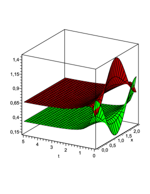
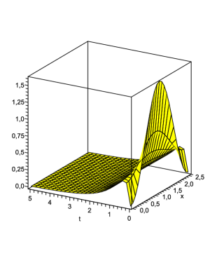
Figure 2: Surfaces representing the components $u$ (green), $v$ (red) and $w$ (yellow) of solution (57) with $\alpha_{0}=1/3,\ \alpha_{1}=0,\ \alpha_{2}=1/4,\ C=8/5,\ \kappa=\sqrt{6}$ of the HGF system (48) with the parameters $d_{1}=2/3,\ d_{2}=1,\ d_{3}=1/2$.

Interestingly, the exact solution (57) with correctly-specified parameters can be used for solving boundary-value problems with typical boundary conditions occurring in biological problems. Let us consider an example. Assuming that the population interaction occurs in the bounded domain

$$\Omega_{\kappa}=\left\{(t,x)\in(0,+\infty)\times\Big{(}\frac{2k\pi}{\kappa},\frac{2(k+1)\pi}{\kappa}\Big{)}\right\},\ k\in\mathbb{Z}$$

with no-flux conditions (the zero Neumann conditions) on the boundaries

$$\begin{array}[]{l}x=\frac{2k\pi}{\kappa}:\ u_{x}=v_{x}=w_{x}=0;\\ x=\frac{2(k+1)\pi}{\kappa}:\ u_{x}=v_{x}=w_{x}=0,\end{array}$$

it can be easily identified that the exact solution (57) with $\alpha_{1}=0$ satisfies these conditions. Moreover, if other parameters satisfy the restrictions

$$1\geq\alpha_{0}+\mid\alpha_{2}\mid\ \geq 2\mid\alpha_{2}\mid,\quad d_{1}<d_{2},\quad C\geq\frac{1-\alpha_{0}}{1-\alpha_{0}-\mid\alpha_{2}\mid},$$

then we obtain the plausible picture of the population interaction (see Fig. 2).

So, we again observe the coexistence of farmers and converted farmers and the extinction of hunter-gatherers as a result of the humanity evolution.

Now we turn back to the ODE system (52) and show that its integration reduces to a nonlinear second-order ODE. First of all, the function $\varphi_{2}$ can be expressed from the first equation of (52):

$$\varphi_{2}=1-\frac{\varphi_{1}^{\prime}}{\varphi_{1}}.$$ (59)

Substituting (59) into the third equation of system (52) and integrating the equation obtained, we arrive at

$$\varphi_{3}=\left(Ce^{-t}-\frac{\alpha_{0}(d_{1}-d_{2})}{d_{1}-d_{3}}\right)\varphi_{1}.$$ (60)

Now the second equation of (52) can be rewritten in the form

$$\begin{array}[]{l}\varphi_{1}^{\prime\prime}-\frac{d_{1}+d_{2}-2d_{3}}{d_{1}-d_{3}}\frac{{\varphi_{1}^{\prime}}^{2}}{\varphi_{1}}+\left(\frac{\alpha_{0}(d_{1}-d_{2})}{d_{1}-d_{3}}-Ce^{-t}\right)\varphi_{1}\varphi_{1}^{\prime}\\ +\frac{d_{2}-d_{3}}{d_{1}-d_{3}}\varphi_{1}^{\prime}+Ce^{-t}{\varphi_{1}}^{2}=0.\end{array}$$ (61)

So, having the general solution of the second-order ODE (61), one easily transforms one into the general solution of the ODE system (52) using formulae (59)–(60).

ODE (61) is still a complicated nonlinear equation. To the best of our knowledge, its general solution is unknown. So, we applied additional restrictions in order to construct solutions of ODE (61). For instance, the general solution of (61) with $C=0$ can be derived by reducing to a first-order ODE. As a result, we obtain

$$t+t_{0}=\int\left(\varphi_{1}-C_{1}\varphi_{1}^{\frac{d_{1}+d_{2}-2d_{3}}{d_{1}-d_{3}}}-\alpha_{0}\varphi_{1}^{2}\right)^{-1}d\varphi_{1}.$$ (62)

Here $C_{1}$ and $t_{0}$ are arbitrary constant and the latter can be removed by the time shift $t+t_{0}\rightarrow t.$ The integral in (62) is expressed in terms of elementary functions if some further restrictions hold. Examples are presented below.

In the case $C_{1}=0$, the function $\varphi_{1}(t)$ has the form

$$\varphi_{1}(t)=\frac{\pm e^{t}}{1\pm\alpha_{0}e^{t}}.$$ (63)

In the case $C_{1}\neq 0$, we may set $2d_{3}=d_{1}+d_{2}$, so that the general solution takes the form

$$\varphi_{1}(t)=\left\{\begin{array}[]{l}\frac{1}{2\alpha_{0}}-\frac{\sqrt{4\alpha_{0}C_{1}-1}}{2\alpha_{0}}\tan\frac{\sqrt{4\alpha_{0}C_{1}-1}\,t}{2},\ \mbox{if}\ 4\alpha_{0}C_{1}>1,\ \alpha_{0}\neq 0,\vskip 6.0pt plus 2.0pt minus 2.0pt\\ \frac{1}{2\alpha_{0}}+\frac{\sqrt{1-4\alpha_{0}C_{1}}}{2\alpha_{0}}\tanh\frac{\sqrt{1-4\alpha_{0}C_{1}}\,t}{2},\ \mbox{if}\ 4\alpha_{0}C_{1}<1,\ \alpha_{0}\neq 0,\vskip 6.0pt plus 2.0pt minus 2.0pt\\ \frac{2+t}{2\alpha_{0}t},\ \mbox{if}\ 4\alpha_{0}C_{1}=1,\ \alpha_{0}\neq 0,\vskip 6.0pt plus 2.0pt minus 2.0pt\\ \pm e^{t}+C_{1},\ \mbox{if}\ \alpha_{0}=0.\end{array}\right.$$ (64)

Thus, substituting (63) and (64) into (59)–(60), one easily obtains exact solutions of the ODE system (52). Having the known functions $\varphi_{i}(t),\ i=1,2,3,$ we readily construct the exact solutions of the HGF system (10) using formulae (50) if $d_{1}>d_{3}$ and (51) if $d_{1}<d_{3}.$

Let us consider, for example, the case $4\alpha_{0}C_{1}<1$ in detail. Straightforward calculations lead to

$$\begin{array}[]{l}\varphi_{1}=\frac{1}{2\alpha_{0}}+\frac{\sqrt{1-4\alpha_{0}C_{1}}}{2\alpha_{0}}\tanh\frac{\sqrt{1-4\alpha_{0}C_{1}}\,t}{2},\vskip 6.0pt plus 2.0pt minus 2.0pt\\ \varphi_{2}=1-\frac{1-4\alpha_{0}C_{1}}{2\cosh^{2}\frac{\sqrt{1-4\alpha_{0}C_{1}}\,t}{2}\Big{(}1+\sqrt{1-4\alpha_{0}C_{1}}\tanh\frac{\sqrt{1-4\alpha_{0}C_{1}}\,t}{2}\Big{)}},\vskip 6.0pt plus 2.0pt minus 2.0pt\\ \varphi_{3}=-1-\sqrt{1-4\alpha_{0}C_{1}}\tanh\frac{\sqrt{1-4\alpha_{0}C_{1}}\,t}{2}.\end{array}$$ (65)

Substituting (65) into ansatz (50), we arrive at the exact solution

$$\begin{array}[]{l}u(t,x)=\left(\frac{1}{2\alpha_{0}}+\frac{\sqrt{1-4\alpha_{0}C_{1}}}{2\alpha_{0}}\tanh\frac{\sqrt{1-4\alpha_{0}C_{1}}\,t}{2}\right)\Big{(}\alpha_{0}+\alpha_{1}\sin(\kappa\,x)\exp(-d_{1}\kappa^{2}t)\\ \hskip 56.9055pt+\alpha_{2}\cos(\kappa\,x)\exp(-d_{1}\kappa^{2}t)\Big{)},\vskip 6.0pt plus 2.0pt minus 2.0pt\\ v(t,x)=1-\frac{1-4\alpha_{0}C_{1}}{2\cosh^{2}\frac{\sqrt{1-4\alpha_{0}C_{1}}\,t}{2}\Big{(}1+\sqrt{1-4\alpha_{0}C_{1}}\tanh\frac{\sqrt{1-4\alpha_{0}C_{1}}\,t}{2}\Big{)}}-u(t,x),\vskip 6.0pt plus 2.0pt minus 2.0pt\\ w(t,x)=\frac{\exp(-d_{1}\kappa^{2}t)}{\alpha_{0}}\Big{(}1+\sqrt{1-4\alpha_{0}C_{1}}\tanh\frac{\sqrt{1-4\alpha_{0}C_{1}}\,t}{2}\Big{)}\\ \hskip 56.9055pt\times\Big{(}\alpha_{1}\sin(\kappa\,x)+\alpha_{2}\cos(\kappa\,x)\Big{)},\end{array}$$ (66)

of the HGF system (48) with $d_{3}=\frac{d_{1}+d_{2}}{2}$ and $d_{1}>d_{2}$.

Exact solutions of the form (66) does not satisfy the natural requirement of nonnegativity at an arbitrary interval. However, these solutions are nonnegative provided the interval is correctly-specified. For instance, setting $\alpha_{2}=0$ and renaming $\beta_{1}=4\alpha_{0}C_{1},\ \beta_{2}=\frac{\alpha_{1}}{\alpha_{0}}$, we transform solution (66) into

$$\begin{array}[]{l}u(t,x)=\left(\frac{1}{2}+\frac{\sqrt{1-\beta_{1}}}{2}\tanh\frac{\sqrt{1-\beta_{1}}\,t}{2}\right)\Big{(}1+\beta_{2}\sin(\kappa\,x)\exp(-d_{1}\kappa^{2}t)\Big{)},\vskip 6.0pt plus 2.0pt minus 2.0pt\\ v(t,x)=1-\frac{1-\beta_{1}}{2\cosh^{2}\frac{\sqrt{1-\beta_{1}}\,t}{2}\Big{(}1+\sqrt{1-\beta_{1}}\tanh\frac{\sqrt{1-\beta_{1}}\,t}{2}\Big{)}}-u(t,x),\vskip 6.0pt plus 2.0pt minus 2.0pt\\ w(t,x)=\beta_{2}\sin(\kappa\,x)\exp(-d_{1}\kappa^{2}t)\Big{(}1+\sqrt{1-\beta_{1}}\tanh\frac{\sqrt{1-\beta_{1}}\,t}{2}\Big{)},\end{array}$$ (67)

where $\kappa=\frac{\sqrt{2}}{\sqrt{d_{1}-d_{2}}}$, $\beta_{1}<1$ and $\beta_{2}$ is an arbitrary constant.

The components of solution (67) are nonnegative in the domain

$$\Omega_{\kappa}=\left\{(t,x)\in(0,+\infty)\times\Big{(}\frac{2k\pi}{\kappa},\frac{(2k+1)\pi}{\kappa}\Big{)}\right\},\ k\in\mathbb{Z},$$

provided the coefficient restrictions $1>\beta_{1}>\beta_{2}>0$ hold.

Obviously, solution (67) possesses the asymptotical behavior

$$(u,\,v,\,w)\rightarrow\left(\frac{1+\sqrt{1-\beta_{1}}}{2},\,\frac{1-\sqrt{1-\beta_{1}}}{2},\,0\right)\ \texttt{as}\ t\rightarrow+\infty,$$ (68)

which again implies extinction of the hunter-gatherer population.

Consider the operator $Q^{w}_{3}$. The ansatz corresponding to this operator has the form

$$\begin{array}[]{l}u(t,x)=\varphi_{1}(t)+\frac{d_{1}-d_{3}}{d_{1}-d_{2}}\,w(t,x),\vskip 6.0pt plus 2.0pt minus 2.0pt\\ v(t,x)=\varphi_{2}(t)-\frac{d_{1}-d_{3}}{d_{1}-d_{2}}\,w(t,x),\vskip 6.0pt plus 2.0pt minus 2.0pt\\ w(t,x)=\varphi_{3}(t)\Big{(}\alpha_{0}+\alpha_{1}\sin(\kappa\,x)\exp(-d_{3}\kappa^{2}t)+\alpha_{2}\cos(\kappa\,x)\exp(-d_{3}\kappa^{2}t)\Big{)},\end{array}$$ (69)

if $d_{1}>d_{3}$, and

$$\begin{array}[]{l}u(t,x)=\varphi_{1}(t)+\frac{d_{1}-d_{3}}{d_{1}-d_{2}}\,w(t,x),\vskip 6.0pt plus 2.0pt minus 2.0pt\\ v(t,x)=\varphi_{2}(t)-\frac{d_{1}-d_{3}}{d_{1}-d_{2}}\,w(t,x),\vskip 6.0pt plus 2.0pt minus 2.0pt\\ w(t,x)=\varphi_{3}(t)\Big{(}\alpha_{0}+\alpha_{1}\exp(\kappa\,x+d_{3}\kappa^{2}t)+\alpha_{2}\exp(-\kappa\,x+d_{3}\kappa^{2}t)\Big{)},\end{array}$$ (70)

if $d_{1}<d_{3}$. Here $\varphi_{1}(t),\ \varphi_{2}(t)$ and $\varphi_{3}(t)$ are unknown functions, while $\kappa=\frac{1}{\sqrt{\mid d_{1}-d_{3}\mid}}.$

Ansätze (69) and (70) lead to the reduced system

$$\begin{array}[]{l}\varphi_{1}^{\prime}+\varphi_{1}\left(\varphi_{1}+\varphi_{2}-1\right)-\frac{\alpha_{0}(d_{1}-d_{3})}{d_{1}-d_{2}}\,\varphi_{3}=0,\vskip 6.0pt plus 2.0pt minus 2.0pt\\ \varphi_{2}^{\prime}+\frac{d_{2}-d_{3}}{d_{1}-d_{3}}\,\varphi_{2}\left(\varphi_{1}+\varphi_{2}-1\right)+\frac{\alpha_{0}(d_{2}-d_{3})}{d_{1}-d_{2}}\,\varphi_{3}=0,\vskip 6.0pt plus 2.0pt minus 2.0pt\\ \varphi_{3}^{\prime}+\varphi_{3}\left(\varphi_{1}+\varphi_{2}\right)=0.\end{array}$$ (71)

Similar to the ODE system (52), system (71) is nonlinear and its general solution is unknown. However, some particular solutions can be derived under additional assumptions. For example, assuming a linear functional dependence between the functions $\varphi_{1}$ and $\varphi_{2}$, we have found the following particular solution

$$\begin{array}[]{l}\varphi_{1}(t)=\frac{d_{1}-2d_{2}+d_{3}}{2\left(d_{1}-d_{2}\right)}\tanh\frac{t}{4},\vskip 6.0pt plus 2.0pt minus 2.0pt\\ \varphi_{2}(t)=\frac{1}{2}+\frac{d_{2}-d_{3}}{2\left(d_{1}-d_{2}\right)}\tanh\frac{t}{4},\vskip 6.0pt plus 2.0pt minus 2.0pt\\ \varphi_{3}(t)=\frac{d_{1}-2d_{2}+d_{3}}{2\alpha_{0}\left(d_{1}-d_{2}\right)\left(1+e^{\frac{t}{2}}\right)^{2}}.\end{array}$$ (72)

Substituting the functions $\varphi_{1}(t)$, $\varphi_{2}(t)$ and $\varphi_{3}(t)$ into ansätze (69) and (70), one obtains two families of exact solutions of the HGF system (48). In particular, the exact solutions generated by ansatz (69) and formulae (72) have the asymptotic behavior of the form (55). So, these solutions describe such interaction between three populations, which leads to the coexistence of farmers and converted farmers and to the extinction of hunter-gatherers.

3.2 The HGF system (11)

Now we construct exact solutions of the HGF system (11) using the operator $Q^{u}_{4}$. Applying the transformation $a_{1}v\rightarrow v$, we can rewrite system (11) and $Q^{u}_{4}$ in the form

$$\begin{array}[]{l}u_{t}=u_{xx}+u(1-u-v),\\ v_{t}=v_{xx}+v(1-u-v)+a_{1}(u+v)w,\\ w_{t}=d_{3}w_{xx}+a_{3}w(1-w)-a_{4}(u+v)w,\end{array}$$ (73)

$$Q^{u}_{4}=\partial_{x}+g(t,x)\,u\left(\partial_{u}-\partial_{v}\right),$$

where $g(t,x)$ is an arbitrary solution of the Burgers equation $g_{t}=g_{xx}+2gg_{x}$.

Solving the invariance surface condition for the operator $Q^{u}_{4}$, one obtains the ansatz

$$\begin{array}[]{l}u(t,x)=\varphi_{1}(t)\exp\left(\int g(t,x)\,dx\right),\\ v(t,x)=\varphi_{2}(t)-u(t,x),\\ w(t,x)=\varphi_{3}(t).\end{array}$$ (74)

It turns out that ansatz (74) can be rewritten in a simpler form, using the famous Cole–Hopf substitution [24, 19] $g=\frac{f_{x}}{f}$, which reduces the Burgers equation to the linear diffusion equation

$$f_{t}=f_{xx}.$$ (75)

As a result, ansatz (74) takes the form

$$\begin{array}[]{l}u(t,x)=\varphi_{1}(t)f(t,x),\\ v(t,x)=\varphi_{2}(t)-\varphi_{1}(t)f(t,x),\\ w(t,x)=\varphi_{3}(t),\end{array}$$ (76)

where $f(t,x)$ is an arbitrary solution of the linear diffusion equation (75). The reduced system corresponding to the ansatz (76) has the form

$$\begin{array}[]{l}\varphi_{1}^{\prime}=\varphi_{1}\left(1-\varphi_{2}\right),\\ \varphi_{2}^{\prime}=\varphi_{2}\left(1-\varphi_{2}+a_{1}\varphi_{3}\right),\\ \varphi_{3}^{\prime}=\varphi_{3}\left(a_{3}-a_{4}\varphi_{2}-a_{3}\varphi_{3}\right).\end{array}$$ (77)

Thus, an arbitrary solution of the linear diffusion equation (75) generates the exact solution of the HGF system (73) provided $(\varphi_{1},\varphi_{2},\varphi_{3})$ is a solution of the ODE system (77).

Let us construct examples of solutions of the nonlinear system (77). Note that this systems contains an autonomous subsystem for $\varphi_{2}$ and $\varphi_{3}$. Because it is nothing else but the two-component Lotka–Volterra system (without diffusion), which is nonintegrable, we apply a technique used by C and D [15] in order to construct particular solutions. So, assuming $\varphi_{3}=\beta_{1}\varphi_{2}+\beta_{2},$ with $\beta_{1}\neq 0$ and $\beta_{2}$ are arbitrary constants, system (77) can be easily integrated and has nontrivial solutions in two cases. Having $\varphi_{2}$ and $\varphi_{3}$ and solving the first ODE from (77), we obtain the first solution

$$\begin{array}[]{l}\varphi_{1}=C_{2}\,e^{t}\left(1+C_{1}\left(e^{t}-1\right)\right)^{-\frac{1+a_{1}}{1+a_{1}a_{4}}},\vskip 6.0pt plus 2.0pt minus 2.0pt\\ \varphi_{2}=\frac{1+a_{1}}{1+a_{1}a_{4}}\frac{C_{1}e^{t}}{1+C_{1}\left(e^{t}-1\right)},\vskip 6.0pt plus 2.0pt minus 2.0pt\\ \varphi_{3}=\frac{1-a_{4}}{1+a_{1}a_{4}}\frac{C_{1}e^{t}}{1+C_{1}\left(e^{t}-1\right)},\end{array}$$ (78)

if $a_{3}=1$, and the second solution

$$\begin{array}[]{l}\varphi_{1}=C_{2}\,e^{t}\left(1+C_{1}\left(e^{(1+a_{1})t}-1\right)\right)^{-\frac{1}{1+a_{1}}},\vskip 6.0pt plus 2.0pt minus 2.0pt\\ \varphi_{2}=\frac{C_{1}e^{(1+a_{1})t}}{1+C_{1}\left(e^{(1+a_{1})t}-1\right)},\vskip 6.0pt plus 2.0pt minus 2.0pt\\ \varphi_{3}=\frac{1-C_{1}}{1+C_{1}\left(e^{(1+a_{1})t}-1\right)},\end{array}$$ (79)

if $a_{3}=a_{4}-a_{1}-1$ ($C_{1}$ and $C_{2}$ are arbitrary constants).

Thus, substituting the functions $\varphi_{1}(t)$, $\varphi_{2}(t)$ and $\varphi_{3}(t)$ given by formulae (78) and (79) into ansatz (76), one immediately obtains two families of exact solutions of the HGF system (73) involving arbitrary solutions of the linear diffusion equation.

Let us consider in detail the solutions of the form

$$\begin{array}[]{l}u(t,x)=C_{2}\,e^{t}\left(1+C_{1}\left(e^{t}-1\right)\right)^{-\frac{1+a_{1}}{1+a_{1}a_{4}}}f(t,x),\\ v(t,x)=\frac{1+a_{1}}{1+a_{1}a_{4}}\frac{C_{1}e^{t}}{1+C_{1}\left(e^{t}-1\right)}-C_{2}\,e^{t}\left(1+C_{1}\left(e^{t}-1\right)\right)^{-\frac{1+a_{1}}{1+a_{1}a_{4}}}f(t,x),\\ w(t,x)=\frac{1-a_{4}}{1+a_{1}a_{4}}\frac{C_{1}e^{t}}{1+C_{1}\left(e^{t}-1\right)},\end{array}$$ (80)

which arise in the case $a_{3}=1$.

Note that the exact solution (80) includes that constructed in [12] (see formula (3.12) therein) as a particular case. In fact, if one sets $f(t,x)=\exp\left(\alpha^{2}t+\alpha x\right)$ ($\alpha$ is an arbitrary constant) in (80) then the exact solution from [12] is immediately obtained.

We assume that the populations interact in the bounded domain

$$\Omega_{ab}=\Big{\{}(t,x)\in(0,+\infty)\times(a,\ b)\Big{\}},\ a<b\in\mathbb{R}$$

and no-flux conditions (the zero Neumann conditions)

$$\begin{array}[]{l}x=a:\ u_{x}=v_{x}=w_{x}=0;\\ x=b:\ u_{x}=v_{x}=w_{x}=0\end{array}$$ (81)

are imposed.

According to the classical theory of linear diffusion equations, there exist a smooth nonnegative bounded solution, $f_{0}(t,x)$, of equation (75) that satisfies the zero Neumann conditions

$$x=a:\ f_{x}=0,\quad x=b:\ f_{x}=0$$

and the initial condition

$$t=0:\ f=F(x),$$

where $F(x)$ is an arbitrary smooth function such that $0\leq F(x)\leq A$, $A\in\mathbb{R_{+}}$. Moreover, the solution $f_{0}(t,x)$ can be constructed in an explicit form using, e.g., the Fourier method.

Now we realize that the exact solution (80) with $f(t,x)=f_{0}(t,x)$ satisfies the no-flux conditions (81). Moreover, all components are bounded and nonnegative provided the constants in (80) are correctly specified. Indeed, the third component $w$ is smooth, nonnegative and bounded provided $C_{1}>0$ and $a_{4}\leq 1$, while the components $u$ and $v$ possess the same properties if $C_{2}\geq 0$ and is sufficiently small. Having the afore-cited restrictions, we observe the following asymptotical behavior of the exact solution (80)

$$(u,\,v,\,w)\rightarrow\left(0,\,\frac{1+a_{1}}{1+a_{1}a_{4}},\,\frac{1-a_{4}}{1+a_{1}a_{4}}\right)\ \texttt{as}\ t\rightarrow+\infty$$ (82)

if $a_{4}<1$ and

$$(u,\,v,\,w)\rightarrow\left(\frac{C_{2}A_{\infty}(x)}{C_{1}},\,1-\frac{C_{2}A_{\infty}(x)}{C_{1}},\,0\right)\ \texttt{as}\ t\rightarrow+\infty$$

if $a_{4}=1$, provided the condition $\lim\limits_{t\rightarrow+\infty}f_{0}(t,x)=A_{\infty}(x)$ takes place.

Now we present a biological meaning of the exact solution (80) with $f(t,x)=f_{0}(t,x)$ as follows. This solution with $a_{4}<1$ describes such a scenario of interaction between three populations, which predicts the coexistence of converted farmers and hunter-gatherers and the total extinction of initial farmers. This scenario differs from that obtained for the solutions of the HGF system (48) (see formulae (55), (58) and (68)). Interestingly, the asymptotic behavior (82) is in agreement with the results derived in [20] and shown numerically in [21]. In fact, the exact solution (80) is valid for the HGF system (73) with the coefficient restriction $a_{3}=1>a_{4}$. In other words, the self-reproduction rate of hunter-gatherers described by the coefficient $a_{3}$ should be sufficiently high in order to survive. It should be stressed that there are no examples of exact solutions in [20] and [21] but only theorems of existence and numerical solutions. Finally, we note that the density of hunter-gatherers in (80) does not depend on the space variable $x$. This means biologically that the hunter-gatherer diffusion is very high, therefore they disperse uniformly in space, i.e., $w_{xx}\approx 0$.

Setting $F(x)=C_{3}+\cos x$ (here $C_{3}\geq 1$ is an arbitrary constant), the function $f_{0}(t,x)$ can easily be derived and one has the form $f_{0}(t,x)=C_{3}+e^{-t}\cos x$. In this case, the exact solution (80) takes the form

$$\begin{array}[]{l}u(t,x)=C_{2}\left(1+C_{1}\left(e^{t}-1\right)\right)^{-\frac{1+a_{1}}{1+a_{1}a_{4}}}\left(C_{3}e^{t}+\cos x\right),\vskip 6.0pt plus 2.0pt minus 2.0pt\\ v(t,x)=\frac{1+a_{1}}{1+a_{1}a_{4}}\frac{C_{1}e^{t}}{1+C_{1}\left(e^{t}-1\right)}-C_{2}\left(1+C_{1}\left(e^{t}-1\right)\right)^{-\frac{1+a_{1}}{1+a_{1}a_{4}}}\left(C_{3}e^{t}+\cos x\right),\vskip 6.0pt plus 2.0pt minus 2.0pt\\ w(t,x)=\frac{1-a_{4}}{1+a_{1}a_{4}}\frac{C_{1}e^{t}}{1+C_{1}\left(e^{t}-1\right)}.\end{array}$$ (83)

An example of solution (83) (that is defined in the domain $\Omega_{2\pi}=\left\{(t,x)\in(0,+\infty)\times(0,\ 2\pi)\right\}$) with correctly-specified coefficients is presented in Fig. 3.

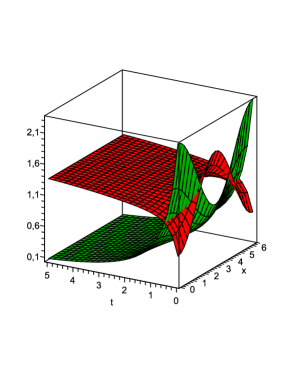
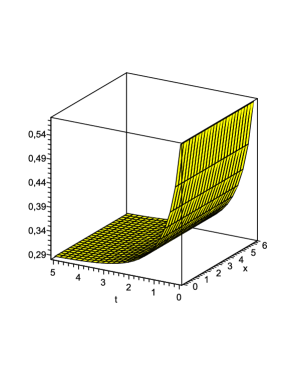
Figure 3: Surfaces representing the components $u$ (green), $v$ (red) and $w$ (yellow) of solution (83) with $C_{1}=2,\ C_{2}=2/3,\ C_{3}=5/2$ of the HGF system (73) with the parameters $a_{1}=3/2,\ a_{3}=1,\ a_{4}=1/2$.

Finally, we note that the exact solutions of the form

$$\begin{array}[]{l}u(t,x)=C_{2}\,e^{t}\left(1+C_{1}\left(e^{(1+a_{1})t}-1\right)\right)^{-\frac{1}{1+a_{1}}}f(t,x),\\ v(t,x)=\frac{C_{1}e^{(1+a_{1})t}}{1+C_{1}\left(e^{(1+a_{1})t}-1\right)}-C_{2}\,e^{t}\left(1+C_{1}\left(e^{(1+a_{1})t}-1\right)\right)^{-\frac{1}{1+a_{1}}}f(t,x),\\ w(t,x)=\frac{1-C_{1}}{1+C_{1}\left(e^{(1+a_{1})t}-1\right)},\end{array}$$ (84)

arising in the case $a_{3}=a_{4}-a_{1}-1$ (see formulae (79)), can be examined in the same way. As a result, the exact solution (84) with a correctly-specified function $f(t,x)=f_{0}(t,x)$ (see the previous page about the function $f_{0}$) has the asymptotical behavior

$$(u,\,v,\,w)\rightarrow\Big{(}C_{1}^{-\frac{1}{1+a_{1}}}C_{2}\ f_{0}^{\infty}(x),\,1-C_{1}^{-\frac{1}{1+a_{1}}}C_{2}\ f_{0}^{\infty}(x),\,0\Big{)}\ \texttt{as}\ t\rightarrow+\infty,$$ (85)

where $f_{0}^{\infty}(x)=\lim\limits_{t\rightarrow+\infty}f_{0}(t,x)$.

Thus, the exact solution (84) with $f(t,x)=f_{0}(t,x)$ describes the scenario of interaction between three populations, which predicts the coexistence of converted farmers and initial farmers and the total extinction of hunter-gatherers. Thus, it is the same scenario as one obtained for solutions of the HGF system (48). Moreover, it is in agreement with the theoretical and numerical results derived in [20, 21] because $a_{3}<a_{4}$.

In conclusion of this section, we present the following observation. Here we were looking for exact solutions of the HGF systems satisfying no-flux conditions on boundaries in domains of the form $\Omega_{k}$ and $\Omega_{ab}$. In other words, the corresponding nonlinear boundary value problems (BVPs) were solved. It means, that the HGF systems (48) and (73) supplied by the zero Neumann conditions are conditionally invariant w.r.t. the corresponding $Q$-conditional symmetries. We note that the rigorous definition of conditional symmetry of BVP was firstly formulated in [16] and one is a nontrivial extension of earlier definitions of Lie symmetry of BVP [6]. However, a complete description of Lie and conditional symmetries of BVPs with governing system (1) is a highly nontrivial problem and lies beyond the scope of paper.

4 Discussion

In this work, $Q$-conditional (nonclassical) symmetries of the HGF system (1) are constructed in a so-called no-go case. We point out that the $Q$-conditional symmetries in the regular case, when $\xi^{0}\not=0$ in (4), were earlier identified in [14]. As the no-go case is more complicated, a new definition was established in order to make essential progress in search for $Q$-conditional symmetries. Applying a new algorithm based on Definition 2, we have proved Theorem 1 giving a complete description of $Q$-conditional symmetries of the first type. The symmetries obtained do not coincide with those derived in [14], i.e. they are new.

All the $Q$-conditional symmetries of the first type listed in Theorem 1 can be applied to construct exact solutions of the corresponding HGF systems of the form (1). Here we have examined two special cases (1), when the corresponding system admits either the symmetry operators $Q^{u}_{3}$ and $Q^{w}_{3}$, or the operator $Q^{u}_{4}$.

Note that the HGF system (48) admitting the symmetry operators $Q^{u}_{3}$ and $Q^{w}_{3}$ has the same structure as a system examined in [14]. The only difference is such that the third equation in system (3.2) [14] contains the terms $-\frac{d_{3}}{d_{1}}uw-\frac{d_{3}}{d_{1}}vw$ (with $d_{3}\not=d_{1}$) instead of $-uw-vw$. However, the exact solutions obtained for HGF system (48) have essentially different structure than those derived for system (3.2) [14].

Moreover, some of the solutions derived in Section 3 possess attractive properties allowing us to provide a plausible archeological interpretation (following the terminology used in [21], it is reasonable to replace ‘biological’ by ‘archeological’). As it is shown by numerical simulations in [21], a typical asymptotic behavior of solutions of the HGF system (1) with the no-flux boundary conditions has either the form (55), or

$$(u,\,v,\,w)\rightarrow(0,\,v_{0},\,w_{0})\ \texttt{as}\ t\rightarrow+\infty,$$ (86)

where $v_{0}$ and $w_{0}$ are expressed via the system coefficients. The solutions derived in Subsection 3.1 possess (under the relevant restrictions) only the asymptotic behavior (55) (obviously (58) and (68) are the same formulae up to notations). It is in agreement with the numerical results obtained in [21] because we examined the HGF system (1) with $a_{3}=0$ (see system (10)). It means that the case $a_{3}<a_{4}=a_{5}$ was studied, which predicts the extinction of hunter-gatherers.

In order to construct exact solutions with the asymptotic behavior (86) and to compare with the results obtained in the recent studies [20, 21], it is necessary to examine the HGF system (1) with $a_{3}>a_{4}=a_{5}$. Such systems occur among systems (8) and (11), which possess nontrivial $Q$-conditional symmetries. Here we restricted ourselves on examination of the HGF system (11) because $d_{1}=d_{2}$ is assumed in [20] and [21]. Thus, using the $Q$-conditional symmetry operator $Q^{u}_{4}$, two families of exact solutions were constructed in Subsection 3.2. In particular, it was shown how an exact solution of the form (80) satisfying the no-flux conditions (81) at a bounded interval $\Omega_{ab}$ can be constructed. Moreover, the solution has the asymptotical behavior (82) provided $a_{4}<a_{3}=1$ in the HGF system (11). Using archeological terminology, this solution predicts the coexistence of converted farmers and hunter-gatherers and the total extinction of initial farmers. It is in agreement with theoretical and numerical results obtained in [20, 21].

Exact solutions of the form (84) do not satisfy the asymptotical condition (86) (independently on a specific form of the function $f(t,x)$). On the other hand, these solutions with a correctly-specified function $f(t,x)$ have the asymptotical behavior (85). Thus, such solutions predict the coexistence of initial and converted farmers and the total extinction of hunter-gatherers. It is again in agreement with the results of [20] and [21] because our solutions are valid for the HGF system (11) with the restriction $a_{3}=a_{4}-a_{1}-1$ , hence $a_{4}>a_{3}$. Interestingly, the multiplier $f_{0}^{\infty}$ in (85) can be a function of the space variable $x$, hence a spatial segregation of initial and converted farmers may occur as $t\rightarrow+\infty$.

Acknowledgments
The authors acknowledge a partial financial support within the framework of the priority program for research and scientific-and-technical (experimental) development of the mathematical department of the NAS of Ukraine in 2022–2023 (Reg. No 0122U000670).

References

- [1] Aoki, K.: A three-population wave-of-advance model for the European early Neolithic. PLoS One 155, e0233184 (2020)
- [2] Aoki, K., Shida, M., Shigesada, N.: Travelling wave solutions for the spread of farmers into a region occupied by hunter-gatherers. Theor. Popul. Biol. 50, 1–17 (1996)
- [3] Arrigo, D.J., Ekrut, D.A., Fliss, J.R., Long, Le.: Nonclassical symmetries of a class of Burgers’ systems. J. Math. Anal. Appl. 371, 813–820 (2010)
- [4] Barannyk, T.: Symmetry and exact solutions for systems of nonlinear reaction-diffusion equations (in Ukrainian). Proc. Inst. Math. Nat. Acad. Sci. Ukraine 43,80–85 (2002)
- [5] Barannyk, T.: Nonclassical symmetries of a system of nonlinear reaction-diffusion equations. J. Math. Sci. 238, 207–214 (2019)
- [6] Bluman G.W., Anco S.C.: Symmetry and integration methods for differential equations. In: Applied Mathematical Science. Springer, New York (2002)
- [7] Bluman, G.W., Cheviakov, A.F., Anco, S.C.: Applications of Symmetry Methods to Partial Differential Equations. Springer, New York (2010)
- [8] Bluman, G.W., Cole, J.D.: The general similarity solution of the heat equation. J. Math. Mech. 18, 1025–1042 (1969)
- [9] Cherniha, R.: Conditional symmetries for systems of PDEs: new definition and their application for reaction-diffusion systems. J. Phys. A: Math. Theor. 43, 405207 (2010)
- [10] Cherniha, R., Davydovych, V.: Lie and conditional symmetries of the three-component diffusive Lotka–Volterra system. J. Phys. A: Math. Theor. 46, 185204 (2013)
- [11] Cherniha, R., Davydovych, V.: Nonlinear Reaction-Diffusion Systems — Conditional Symmetry, Exact Solutions and their Applications in Biology. Lecture Notes in Mathematics, vol. 2196. Springer, Cham (2017)
- [12] Cherniha, R., Davydovych, V.: A hunter-gatherer–farmer population model: Lie symmetries, exact solutions and their interpretation, Euro. J. Appl. Math. 30, 338–357 (2019)
- [13] Cherniha, R., Davydovych, V.: New conditional symmetries and exact solutions of the diffusive two-component Lotka–Volterra system. Mathematics 9, 1984 (2021)
- [14] Cherniha, R., Davydovych, V.: Conditional symmetries and exact solutions of a nonlinear three-component reaction-diffusion model. Eur. J. Appl. Math. 32, 280–300 (2021)
- [15] Cherniha, R., Dutka, V.: A diffusive Lotka–Volterra system: Lie symmetries, exact and numerical solutions. Ukr. Math. J. 56, 1665–75 (2004)
- [16] Cherniha R., King J.R.: Lie and conditional symmetries of a class of nonlinear (1+2)-dimensional boundary value problems. Symmetry 7, 1410–35 (2015)
- [17] Cherniha, R., Serov, M.: Nonlinear systems of the Burgers-type equations: Lie and Q-conditional symmetries, ansatze and solutions. J. Math. Anal. Appl. 282, 305–328 (2003)
- [18] Cherniha, R., Serov, M., Pliukhin, O.: Nonlinear Reaction-Diffusion-Convection Equations: Lie and Conditional Symmetry, Exact Solutions and their Applications. Chapman and Hall/CRC, New York (2018)
- [19] Cole, J.D.: On a quasi-linear parabolic equation occurring in aerodynamics. Quart. Appl. Math. 9, 225–236 (1951)
- [20] Elias, J., Mimura, M., Mori, R.: Asymptotic behavior of solutions of Aoki–Shida–Shigesada model in bounded domains. Discrete Contin. Dyn. Syst. Ser. B 26, 1917–1930 (2021)
- [21] Fu, S.C., Mimura, M., Tsai, J.C.: Traveling waves for a three-component reaction-diffusion model of farmers and hunter-gatherers in the Neolithic transition. J. Math. Biology 82, 1–35 (2021)
- [22] Fushchych, W.I., Shtelen, W.M., Serov, M.I.: Symmetry Analysis and Exact Solutions of Equations of Nonlinear Mathematical Physics. Kluwer, Dordrecht (1993)
- [23] Hashemi, M.S., Nucci, M.C.: Nonclassical symmetries for a class of reaction-diffusion equations: the method of heir-equations. J. Nonlinear Math. Phys. 20, 44–60 (2013)
- [24] Hopf, E.: The partial differential equation . Comm. Pure. Appl. Math. 3, 201–230 (1950)
- [25] Kamke, E.: Differentialgleichungen. Lösungmethoden and Lösungen (in German). 6-th edn. Leipzig (1959)
- [26] Lie, S.: Über die Integration durch bestimmte Integrale von einer Klasse lineare partiellen Differentialgleichungen (in German). Arch. Math. 6, 328–368 (1981)
- [27] Lie, S.: Algemeine Untersuchungen über Differentialgleichungen, die eine continuirliche endliche Gruppe gestatten (in German). Math. Annalen. 25 (1885)
- [28] Murata, S.: Non-classical symmetry and Riemann invariants. Int. J. Non-Lin. Mech. 41, 242–246 (2006)
- [29] Nucci, M.C.: Iterations of the non-classical symmetries method and conditional Lie-Bäcklund symmetries. J. Phys. A: Math. Gen. 29, 8117–8122 (1996)
- [30] Oliveri, F.: ReLie: a Reduce program for Lie group analysis of differential equations. Symmetry 13, 1826 (2021)
- [31] Saccomandi, G.: A personal overview on the reduction methods for partial differential equations. Note di Matematica 23, 217–248 (2005)
- [32] Torrisi, M., Tracina, R.: Exact solutions of a reaction-diffusion system for Proteus mirabilis bacterial colonies. Nonlinear Anal. RWA 12, 1865–1874 (2011)
- [33] Xiao, D., Mori, R.: Spreading properties of a three-component reaction-diffusion model for the population of farmers and hunter-gatherers. In Annales de l’Institut Henri Poincaré, Analyse non linéaire. 38, 911–951 (2021)
- [34] Zhdanov, R.Z., Lahno, V.I.: Conditional symmetry of a porous medium equation. Phys. D 122, 178–86 (1998)