Thermodynamic limits of sperm swimming precision.

Abstract

Sperm swimming is crucial to fertilise the egg, in nature and in assisted reproductive technologies. Modelling the sperm dynamics involves elasticity, hydrodynamics, internal active forces, and out-of-equilibrium noise. Here we give experimental evidence in favour of the relevance of energy dissipation for sperm beating fluctuations. For each motile cell, we reconstruct the time-evolution of the two main tail’s spatial modes, which together trace a noisy limit cycle characterised by a maximum level of precision $p_{max}$. Our results indicate $p_{max}\sim 10^{2}s^{-1}$, remarkably close to the estimated precision of a dynein molecular motor actuating the flagellum, which is bounded by its energy dissipation rate according to the Thermodynamic Uncertainty Relation. Further experiments under oxygen deprivation show that $p_{max}$ decays with energy consumption, as it occurs for a single molecular motor. Both observations are explained by conjecturing a high level of coordination among the conformational changes of dynein motors. This conjecture is supported by a theoretical model for the beating of an ideal flagellum actuated by a collection of motors, including a motor-motor nearest neighbour coupling of strength $K$: when $K$ is small the precision of a large flagellum is much higher than the single motor one. On the contrary, when $K$ is large the two become comparable. Based upon our strong motor coupling conjecture, old and new data coming from different kinds of flagella can be collapsed together on a simple master curve.

I Swimming with noise

Sperm motility plays a crucial role in sexual reproduction and also serves as a prototype for understanding the physics of microswimmers Lauga and Powers (2009); Elgeti et al. (2015). Its investigation is fundamental to develop new technologies, for instance to improve fertility diagnostics and assisted reproduction techniques Fauci and Dillon (2006). It can also positively influence the field of artificial microswimmers and of microfluidic devices Tsang et al. (2020).

A sperm cell is composed by a large head (spatulate-shaped for bull sperms as those considered here) and a thin whip-like tail called flagellum, whose oscillatory movement sustains a travelling wave from head to tail Lindemann and Lesich (2016). In the last decades, physics has investigated the sperm swimming problem, how it originates from flagellar beating coupled to the fluid dynamics and to the many possible boundary conditions Machin (1958); Elgeti et al. (2010); Gaffney et al. (2011). Different swimming modes have been identified, including planar beating near flat (e.g. air-liquid or liquid-substrate) surfaces, beating with precession when the head is anchored to a point, circular trajectories on a plane, 3d helical in the bulk, etc. Crenshaw (1989).

In modelling, minimal ingredients for swimming of semi-flexible filaments, are an anisotropic Stokes drag and a single travelling wave, e.g. (for small deviations $y(t,s)$ from the straight rod shape at time $t$ and arclength $s\sim x$) $y(t,x)=A\cos(kx-\omega t)$ which guarantees irreversibility of the shape cycle i.e. $y(t,x)\neq y(T-t,x)$ where $T$ is the cycle period, necessary to swim at low Reynolds numbers Gray and Hancock (1955); Purcell (1977). An important element is noise, that is deviations from the average flagellum beating dynamics, which has been previously considered in modelling Jülicher and Prost (1997); Friedrich and Jülicher (2008, 2009); Elgeti et al. (2010) and in experiments, with Chlamydomonas Polin et al. (2009); Goldstein et al. (2009, 2011); Wan and Goldstein (2014); Quaranta et al. (2015) and with sperms Ma et al. (2014). In particular such experimental works have estimated through different methods the quality factor of the phase noise in the beating cycle, a parameter which is strictly connected to the precision studied here, as discussed later. Flagellar fluctuations have been observed to influence self-propulsion Klindt and Friedrich (2015) and synchronization of adjacent filaments Goldstein et al. (2009, 2011); Solovev and Friedrich (2022).

In the present study we show how energy dissipation, an intrinsic quantity for motors at all scales, affects noise in sperm beating, rationalising the problem under the framework of Thermodynamic Uncertainty Relations (TURs) Barato and Seifert (2015); Gingrich et al. (2016); Horowitz and Gingrich (2020) (see Appendix D for a summary of the simplest working principle behind TURs). Remarkably, the connection between power consumption and macroscopic fluctuations leads us to put forward a hypothesis about the collective dynamics of the molecular motors actuating the flagellum.

The sperm axoneme hosts an array of dynein molecules for a total of $N\sim 10^{5}$ motor domains Lindemann (2003); Chen et al. (2015); Gilpin et al. (2020). Each motor converts available ATP molecules into power strokes inducing local bending of the axoneme. Deviations from the average biochemical cycle of a molecular motor occur mainly because of fluctuating times of residence in the different chemical states Bustamante et al. (2001). Less understood is the mechanism of coordination of the $N$ motors necessary to generate the tail’s travelling wave: a widely accepted fact is the presence of some feedback mechanism inducing activation and de-activation of the motors based upon the local bending state Brokaw (2009). The hypothesis that a dynein operates independently of its neighbors is questioned by the observation - in micrographs by scanning electron microscopy, etc. - of non-random grouping of dynein states and by the evidence that interactions between adjacent dyneins may be inevitable because of the size of dynein arms Brokaw (2002); Burgess (1995); Goodenough and Heuser (1982). Our experimental observations about the high amplitude of the noise affecting flagellum beating (comparable to that of a dynein motor) and about the decay of flagellum precision with energy consumption (similar to what happens for a single motor), contribute together to conjecture a strong coupling between the dynamics of adjacent motors proteins. A schematic model for axonemal oscillations under the effect of noisy motor dynamics corroborates our hypothesis.

II Precision of a Brownian motor

We first discuss how to measure “precision”, an observable which has recently attracted a profound interest in non-equilibrium statistical physics, see Fig. 1. For our purpose it is sufficient to consider a system where an angular observable $\theta(t)$ represents the system’s configuration (see Fig. 1a and b). We expect $\theta(t)$ to perform an irreversible stochastic stationary dynamics with average drift $\langle\theta(t)-\theta(0)\rangle=Jt$ and relative dispersion $\langle[\theta(t)-\theta(0)-Jt]^{2}\rangle\sim 2Dt$ for large $t$. We are interested in the precision rate defined as

$$p=\frac{J^{2}}{D}.$$ (1)

The observable $p$ can be understood as the inverse of the typical time $t^{*}=1/p$ separating the diffusive regime $t\ll t^{*}$ ($Dt\gg(Jt)^{2}$) from the ballistic regime $t\gg t^{*}$ (see Fig. 1c and its insets).

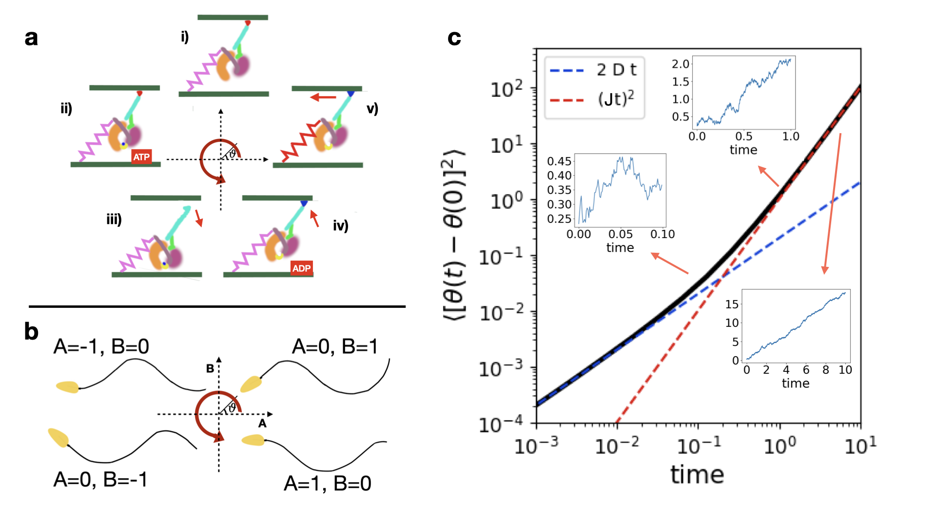
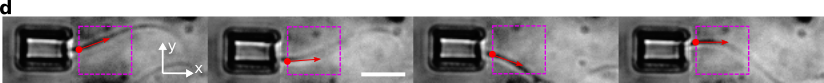
Figure 1: Precision of stochastic clocks. Examples - in different systems - of the coarse-grained coordinate $\theta(t)$ useful to define the precision $p$ of Brownian clocks. a, Sketch of the supposed chemical cycle of the dynein ATP-ase, anti-clockwise starting from the top: i) “rest” (apo) state, ii) ATP-binding; iii) detachment of the stalk; iv) ATP $\to$ ADP+P reaction with re-joining of the stalk to the upper substrate, in a forward position; v) stroke of the linker (red spring) with consequent dragging of the upper substrate. b, Sketch of the elasto-mechanical cycle of a sperm cell, the tail shape is approximated by a curve close to $A(t)\cos(kx)+B(t)\sin(kx)$. c, Mean squared displacement from a trajectory generated by the numerical integration of equation $\dot{\theta}=J+\sqrt{2D}\eta(t)$ with $\eta(t)$ white noise with unitary amplitude, with $J=1$ and $D=0.1$. The insets show the trajectory $\theta(t)$ with a different time-range, i.e. c1) $t\in[0,0.1]$, c2) $t\in[0,1]$, c3) $t\in[0,10]$. It is evident how the mean current $\overline{\dot{\theta}}=J$ can be appreciated only at times much larger than $1/p=D/J^{2}$. d, successive snapshots (taken at a distance $0.04$ seconds with an optical microscope, see Appendix A) of the tail dynamical sequence in a caged sperm experiment: the purple box represents the region of interest, the red dot and red arrow identify the parameters $a,b$ (y-position and slope of the tail close to the origin, respectively) which approximate $A,B$ in Eq. (3), here corresponding to $(A,B)\sim(0,1)\to(-1,0)\to(0,-1)\to(1,0)$. The white arrows indicate $\hat{x}$ and $\hat{y}$ directions ($\hat{z}$ direction is perpendicular to both). The white scalebar represents $10\mu m$.

The quantity $p$ has been demonstrated - through the so-called Thermodynamic Uncertainty Relation (TUR) Barato and Seifert (2015); Gingrich et al. (2016); Horowitz and Gingrich (2020) to be bounded from above by the entropy production rate, or in practical terms (for the purpose of steady isothermal molecular motors) the motor’s energy consumption rate $\dot{W}$ in thermal units:

$$p\leq p_{TUR}=\frac{\dot{W}}{k_{B}T}.$$ (2)

The ratio $\mathcal{Q}=p/p_{TUR}\leq 1$ can be considered as a motor’s figure of merit. Estimates of $p$ through Markovian models informed by experimental data Hwang and Hyeon (2018) suggest that several molecular motors work not far from their optimum, or at least close to its order of magnitude ($\mathcal{Q}\geq 0.1$). In the following we present a method to estimate $p$ and we apply it to experiments with bulls’ sperm cells (see Fig. 1b and d). Notwithstanding its physical relevance, the quantity $p$ has not been discussed for microswimmers, even if its estimate can be deduced from other variables in previous works. Quantities which are strictly related to $p$ are the dissipation time Falasco and Esposito (2020) and the quality factor $q=J/(2D)=p/(2J)$, which has been measured within a similar approach for Chlamydomonas flagella in Polin et al. (2009); Goldstein et al. (2009, 2011); Wan and Goldstein (2014); Quaranta et al. (2015) and for bull sperms in Ma et al. (2014), although never compared to energy dissipation and or discussed within the framework of TURs.

III Precision of sperm beating

We adopt a coarse-graining protocol that reduces the space of possible shapes of the flagellum into two coordinates, the minimum for the existence of irreversible limit cycles. We improve the quality of image tracking and disentangle the simplest mode of sperm movement - that is the planar one - with the following technique: each observed sperm has its head trapped in a microcage printed by 2-photon microlitography, see Fig.  1d and Appendix A. The cell cannot spin and the flagellum beats on the $\hat{xy}$ plane. While the most common swimming strategy of sperm cells is helical Rikmenspoel et al. (1960); Crenshaw (1989), planar movement is typically observed close to a surface and can lead to circular paths Woolley (2003); Nosrati et al. (2015); Saggiorato et al. (2017), here prevented by the cage. The sperm’s center of mass has a very limited dynamics in the $\hat{xz}$ plane but can oscillate along the transverse $\hat{y}$ direction; the body, entirely free, performs planar tail beating which pushes the body into the cage making the escape probability negligible. As a direct consequence of tail beating, the head is also observed to oscillate: our main results are obtained by tail tracking, while in the Supplementary Information we confirm our conclusions by tracking the head, see sup and its Fig. S1.

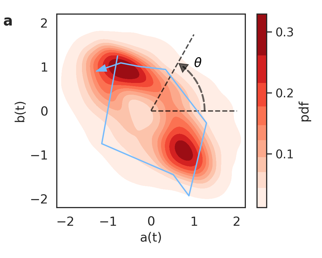
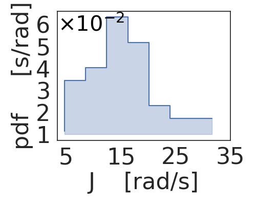
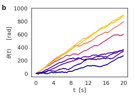
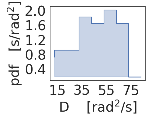
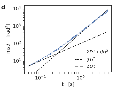
l37.5ptt11pt r17ptb29pt
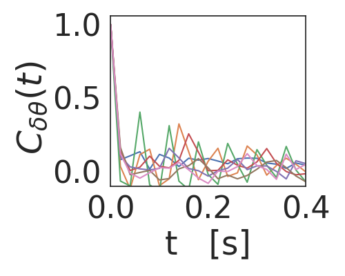
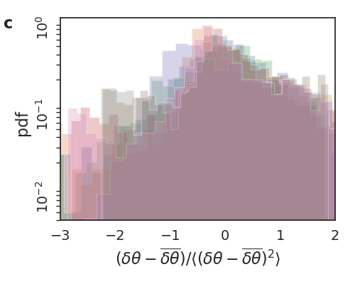
l33ptt9pt l36ptb27pt

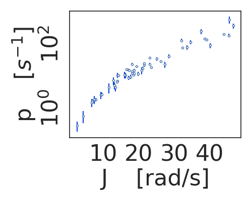
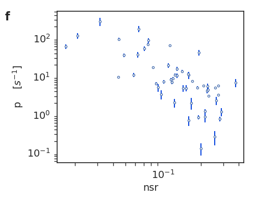
Figure 2: Extracting precision from tail tracking. a, Histogram of the positions in the plane $a(t),b(t)$ for the $12$ sperms with precision $p>20s^{-1}$. The light-blue curve traces the $a(t),b(t)$ path for a particular sperm in $0.2$ seconds ($10$ frames). b, Integrated phase-space current $\theta(t)$ for a few observed sperms. The inset shows the probability density (pdf, over all observed sperms) of the average current $J$. c, Pdf (over $20$ seconds acquisition), for a few sperms, of $\delta\theta=\theta(t+dt)-\theta(t)$ (shifted by the mean and scaled by the standard deviation), where $dt=0.02$ seconds. The inset shows a few autocorrelations $C(t)=\langle\tilde{\delta\theta}(t)\tilde{\delta\theta}(0)\rangle$ where $\tilde{\delta\theta}=\delta\theta-\langle\delta\theta\rangle$. d, Mean squared displacement of $\theta(t)$ for a given sperm, and its fit according to the model $msd(t)=2Dt+(Jt)^{2}$. The inset shows the pdf of diffusivity $D$ over all observed sperms. e, Diffusivity $D$ versus average current $J$ together with decaying exponential fit $D\sim 10^{2}*e^{-J/25}s^{-1}$. f, Precision $p$ versus the noise-to-signal ratio (nsr) computed from the signals $a(t)$ and $b(t)$. The inset shows the $p$ versus the current $J$. Error bars for $J$ and $D$ (in plots e and f) denote $3$ times the standard deviation of $J$ and $D$ estimated when fitting the msd by chi-square optimization. Data come from the observation of $54$ different sperm cells, if not differently specified.

Referring to Fig. 1d, our region of interest (ROI) tracks less than half of the observed beating wavelength. After image processing (see Appendix B) each tail’s image is fitted through a second order polynomial $y(x,t)=a(t)+b(t)x+c(t)x^{2}$ (see also Movie in the Supplementary Information sup ). Under the assumption that the ROI contains less than half wavelength (and therefore $y(x,t)$ has at most one extremal point), $a(t)$ and $b(t)$ are - but for multiplicative constants - fair approximations of the coefficients $A(t)$ and $B(t)$, respectively, of a mode expansion

$$y(x,t)\approx A(t)\cos(kx)+B(t)\sin(kx)\\ \sim_{x\to 0}A(t)+kB(t)x+\mathcal{O}(x^{2})$$ (3)

Such a kind of shape approximation and the consequent coarse-graining of the planar flagellum dynamics into two main coordinates $A,B$ has been used for bull sperms Ma et al. (2014), with Chlamydomonas flagella Polin et al. (2009); Goldstein et al. (2009, 2011); Wan and Goldstein (2014); Quaranta et al. (2015) and with human sperms Saggiorato et al. (2017). A similar approach to the breakdown of detailed balance in flagella has been adopted in experiments with Chlamydomonas Battle et al. (2016), with filaments in actin-myosin networks Gladrow et al. (2017), with C. elegans worms Stephens et al. (2008). A general perspective about this strategy is discussed in a recent review Gnesotto et al. (2018). In experiments of this kind, however, precision and TUR are rarely considered Li et al. (2019); Roldán et al. (2021).

For the purpose of estimating $p$ for each cell, we first apply a filter to the $a(t),b(t)$ time series in order to remove low-frequency drifts, including average, and normalise the data to have a standard deviation of $1$. We observe that the two coordinates exhibit almost harmonic oscillations at a similar frequency $f\sim 6-8Hz$ (see spectra in Appendix B, Fig. 6b,c) but with a phase delay $\Delta(t)$ that fluctuates around a steady non-zero value (Fig. 6a). This delay allows us to reconstruct the angle $\theta(t)$ in the plane $a(t),b(t)$, see Fig. 2a, and finally measure the average phase-space current $J=\langle\theta(t)\rangle/t$, see Fig. 2b. Apart from a few noise dominated cells where $J$ is small and negative we find $J>0$, as expected from the geometrical interpretation of $a(t)$ and $b(t)$ in terms of the main modes of the tail’s shape. A negative $J$ would correspond to a waveform travelling in a direction that is incompatible with forward swimming. We stress that the cumulative phase-space angle $\theta(t)$ is proportional to the number of performed cycles of the sperm’s tail shape dynamics. The average current $|J|$ is related to the beating frequency $f$ in a subtle way: in fact, the growth of $\theta(t)$ is influenced not only by the oscillation of $a(t)$ and $b(t)$ but also by the sign of their phase delay $\Delta$. Failures to guarantee a constant sign of $\Delta$ imply ineffective beatings, i.e. uncoordinated oscillations which do not contribute to the growth of $\theta(t)$, leading to $|J|\leq J_{max}=2\pi f$.

Fluctuations of the rotation speed $\dot{\theta}(t)-J$ are well visible in our experiment, see Figs. 2b and c, and represent departures from the average shape cycle $\theta_{ideal}(t)=Jt$. They are in part due to real dynamical noise (“stochastic deviations”) and in part to the fact that the real shape dynamics is slightly different from the approximated one (“deterministic deviations”). Since deterministic deviations are periodic and each experiment includes hundreds of beating periods, their contribution to the diffusivity $D$ can be safely neglected for our purpose. The main origin of stochastic deviations is non-equilibrium fluctuations, acting both on the fluid surrounding the flagellum and on the working cycle of the thousands of molecular motors actuating the flagellum. At low Reynolds numbers the first effect is negligible (see Appendix B.2).

We empirically find a good fitting model for the mean squared displacement (msd) $\langle[\theta(t+\tau)-\theta(t)]^{2}\rangle\sim J\tau+2D\tau^{2}$ (averaged over $t$ along each whole experiment), see Fig. 2d for an example. Alternative ways to estimate the diffusivity are discussed in Ma et al. (2014), we have considered them for our experiment, finding a substantial agreement, see the Supplementary Information sup with Fig. S2. In Fig. 2e we show the relation between diffusivity $D$ and average current $J$ displaying an average decay but with wide population variability. In Fig. 2f we plot the measured values of $p$ in a large set of experiments, as function of the noise-to-signal ratio (defined as the ratio between the peak of the spectrum and its average at frequencies higher than the oscillation frequency, see Fig. 6 in the Appendix B), and - in the inset - versus $J$. Our first main conclusion is that $p$ takes values in the approximate range $0-p_{max}$ with $p_{max}\approx 10^{2}s^{-1}$. Moreover we see that it roughly decreases with the noise-to-signal ratio and it roughly increases with $J$. A visual inspection of the extremal cases, i.e. those close to $0$ and those close to $p_{max}$, confirm that they correspond to chaotic motion and to almost regular periodic motion respectively.

IV Sperm precision is much smaller than the TUR bound

Direct empirical estimates of the energy consumption - through respiration and glycolysis - for various types of sperms, gave figures in the range of $10^{7}\div 10^{8}$ $k_{B}T/s$, see Appendix B Brokaw (1967); Rikmenspoel et al. (1969); Chen et al. (2015). Theoretical estimates for the power produced by a micro-swimmers are given by the Taylor formula, here adapted for bull sperms Rikmenspoel et al. (1969):

$$\dot{W}_{prod}\approx\pi^{3}\eta Lf^{2}\beta^{2},$$ (4)

where $\beta$ is the tail beating amplitude, $L$ is the tail length and $\eta$ the host fluid viscosity (we have assumed, in the original Taylor’s formula, the cross section of the flagellum to be $\sim 0.2\mu m$ and the tail wavelength $\sim 35\mu m$). We set $\beta=5\mu m$ (only weakly varying with external conditions in our range, see Rikmenspoel (1984)), $L=60\mu m$, $\eta=10^{-3}\textrm{Pa}\cdot s$. The accepted order of magnitude of sperm’s efficiency is $\sim 10-25\%$ Brokaw (1966, 1975); Nicastro et al. (2006); Carvalho-Santos et al. (2011); Klindt et al. (2016); Pellicciotta et al. (2020), giving values which are compatible with experimental estimates $\dot{W}\approx 10^{8}k_{B}T/s$ when $f=20Hz$ at $37^{\circ}C$. In our experiments at room temperature $\sim 20^{\circ}C$ the typical beating frequency is $6-7Hz$, leading to $\dot{W}\approx 10^{7}k_{B}T/s$, and therefore $p_{TUR}=10^{7}s^{-1}$. It is clear that all these figures rest in a much narrower range if the normalised consumption rate is considered $\dot{W}/f^{2}\approx 2-5\cdot 10^{6}k_{B}Ts$. In conclusion the bound Eq. (2) largely overestimates our measured maximum precision, with $\mathcal{Q}_{macro}=p_{max}/p_{TUR}\sim 10^{-5}$. In the following we propose an interpretation of this result.

An intriguing observation concerns the maximum precision, computed from empirical data-informed models, of the dynein molecular motors $p_{d}$ Hwang and Hyeon (2018) which is close to the maximum values we have measured for the whole flagellum $p_{d}\sim p_{max}$ . Our interpretation of the similarity between those two figures is the following. Let us denote with $\theta_{i}(t)$ the integrated current - in the space of motor configurations - in the time $t$ for the $i$-th dynein motor. In both the systems (sperm’s flagellum and dynein) the current integrated in time counts the cumulative number of performed cycles in the configuration space. We conjecture that - in a given amount of time - the number of cycles in the configuration space of the sperm’s flagellum is proportional to the number of cycles in the motor configuration space of any molecular motor in that flagellum, i.e. $\theta(t)\approx C\theta_{i}(t)$, $\forall i\in[1,N]$, with possible $i$-dependent corrections which rapidly vanish with $t$. The result of this conjecture is that the precision of variable $\theta(t)$ is close to the precision of variables $\theta_{i}(t)$ for any $i$. The biological meaning of our conjecture is that a long-range coordination among molecular motors inside the flagellum, quite an accepted fact in the literature Brokaw (2009), affects also fluctuations. In order to make our conjecture more robust, we proceed along two different roads: a new theoretical model and a second experiment.

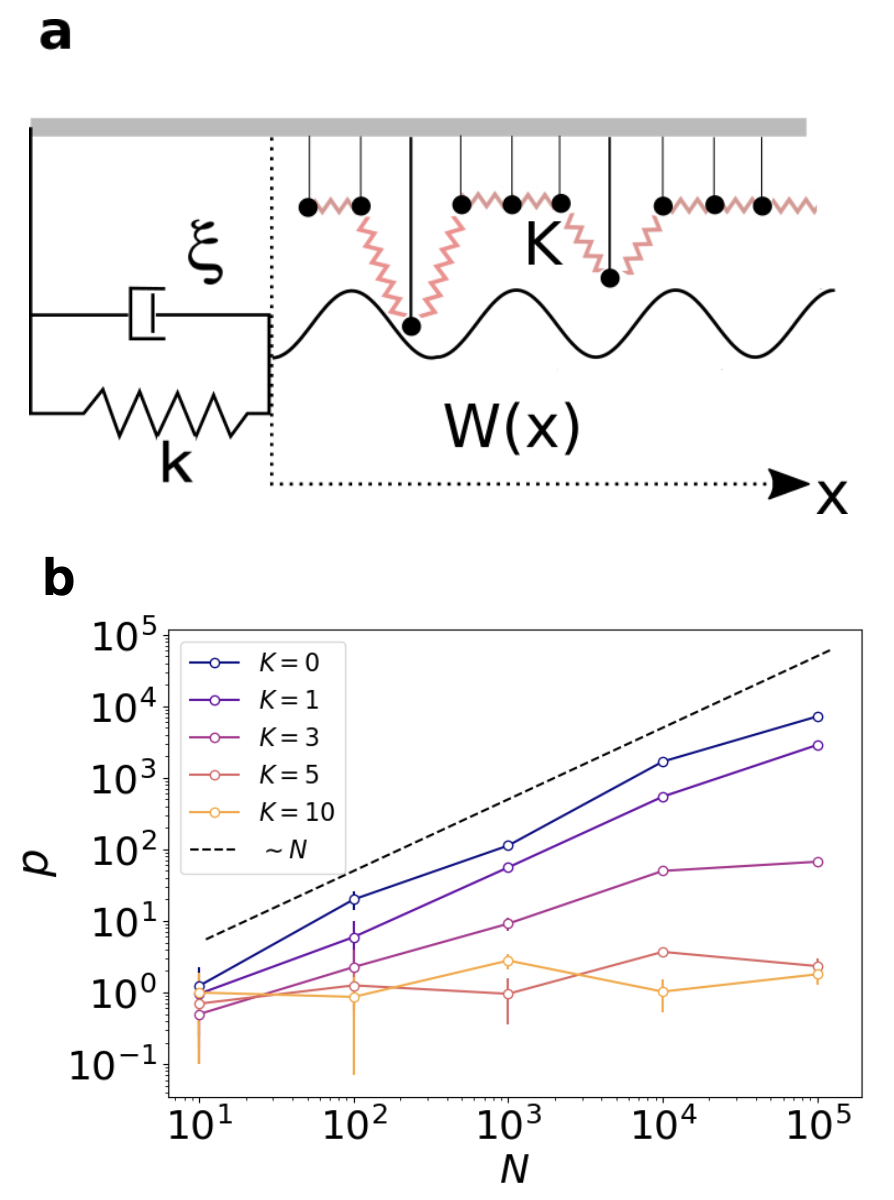
Figure 3: Theoretical model. a, sketch of the model; b, precision $p$ versus number of motors $N$ for different choices of the coupling parameter $K$, showing the $O(N)$ scaling for uncoupled motors ($K=0$) and the $O(1)$ scaling for large $K$. In all the simulations we have used $\alpha=\eta=0.5$, $k/(\xi\Omega)=10$, $\alpha NU_{0}/(\Omega\ell^{2}\xi)=0.6$. The error bars are obtained to error propagation based upon the error in the measurement of $D$. Such error is the estimated standard deviations of $D$ in the non-linear least squares fit of the exponential decay of the phase correlation (see Appendix C).

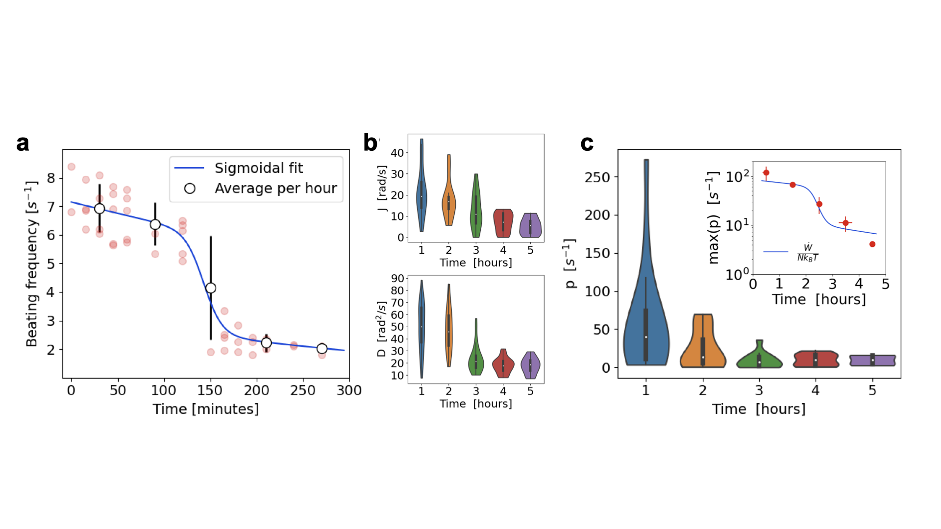
Figure 4: Sperm precision and thermodynamics. Observations for caged sperms in experiments within a sealed chamber. a, Decay of beating frequency (as measured from the spectrum peak of $a(t)$ and $b(t)$), with time. The averages values of the frequencies at each hour of experiment are also marked as white circles, together with a sigmoid-like fit $f(t)=c_{1}e^{-c_{2}t}s(t)+c_{3}e^{-c_{4}t}[1-s(t)]$ with sigmoid $s(t)=[1+e^{(t-t_{0})/\tau}]^{-1}$ and best fit values $t_{0}=143$, $\tau=10.2$, $c_{1}=7.1$, $c_{2}=1.1\times 10^{-3}$, $c_{3}=3.5$, $c_{4}=2\times 10^{-3}$. b, reduction of average current and diffusivity along time, shown as violin plots each from a hour bin (e.g. $1$ means all observation done in the $1$st hour, etc.). c, decay of precision with time, again in the form of a violin plot. The inset shows the decay of $p_{max}$ (estimated as the average of the top $25\%$ population) together with the normalised (by $N=10^{5}$) power consumption extracted by the Taylor formula, eq. (4) using the frequency decay fit shown in Fig. 3a, with amplitude fixed at the average observed value $5.2\mu m$. Error bars represent standard deviations normalised by square root of the number of data in the aforementioned percentile. The sizes of samples in the plots of frames b and c are: 41 sperms in the 1st hour, 24 in the 2nd hour, 34 in the 3rd hour, 25 in the 4th hour and 16 in the 5th hour.

V A model with strongly coupled motors

A first clue in support of our conjecture comes from the numerical analysis of a theoretical model for the motor-actuated flagellar dynamics, extensively studied in Jülicher and Prost (1997); Guérin et al. (2011a, b), modified here through the introduction of a coupling term between adjacent motors. The model is depicted in Fig. 3a and is described in details in the Appendix C. It consists of a filament with $N$ motors. Each motor acts on the filament through an interaction potential, and performs a stochastic attachment/detachment dynamics which breaks detailed balance as if consuming ATP. The motor position $X$ oscillates under the joint effect of the forces of the attached motors and of an external elastic force $\xi\dot{X}(t)=-\partial_{X}\sum_{i}s_{i}U[x_{i}-X(t)]-\kappa X$ with $s_{i}\in\{0,1\}$ representing the detached-attached status of $i$-th motor, the motor-filament potential $U(x)=U_{0}[1-\cos(2\pi x/\ell)]$, viscosity $\xi$ and elastic constant of the external spring $\kappa$. The elastic force here could represent the effect of the cage but in previous studies was introduced just to simplify the mathematics of the problem, it is not crucial for the model’s phenomenology Guérin et al. (2011a). The variables $s_{i}$ jump from $0$ to $1$ and back according to a Poisson process. In the original model the probability rates of such a process depended only upon the local motor-filament potential, so that the fluctuations of the jump dynamics of each motor was independent from nearby motors: for this reason the amplitude of the macroscopic noise was observed to decrease with $N$ Ma et al. (2014). Here we employ a binding potential $K(s_{i}-s_{i+1})^{2}$ that correlates the states $s_{i}$ and $s_{i+1}$ of adjacent motors. Increasing $K$ (from the case $K=0$ which corresponds to the original version) drastically changes the behavior of the model, in particular resulting in a much stronger macroscopic noise, i.e. a largely faster decay of the phase correlation, see Fig. 7 in the Appendix C.

In Fig. 3b we draw our main new conclusion, measuring the precision $p=\omega^{2}/D$ where $\omega$ is the average oscillation frequency and $D$ the diffusivity deduced from the decay of phase correlation Ma et al. (2014). When $K=0$ the precision grows linearly with $N$, in agreement with what already observed in Ma et al. (2014) and with the reasonable argument that the $N$ random independent fluctuations of the motor phases contribute with a variance $1/N$ to the fluctuations of the macroscopic phase. However, the noise reduction due to the growth of $N$ disappears at large $K$: when $K$ increases the size-scaling of $p$ goes from $p\sim O(N)$ to $p\sim O(1)$. This result amounts to say that the precision of the whole flagellum becomes comparable to the precision of the single motor when $K$ is large enough, as in the experiment. On the other side, the energy consumption (ATP consumed per cycle and per motor) increases with $N$, mostly independently of the coupling strength. The ratio between precision $p\sim O(1)$ and energy consumption $\dot{W}\sim N$ therefore decreases as $1/N$, in fair agreement with our experimental observations.

VI Experiment under oxygen deprivation

Experimentally, we reconsider the TUR, Eq. (2). For a single dynein motor, in fact, it establishes a close upper bound: $\mathcal{Q}_{micro}=p_{d}/(\dot{W}_{dynein}/k_{B}T)\gtrsim 10^{-1}$. The closeness of the bound suggests that a variation of energy consumption must reflect into a proportional variation of dynein’s precision, confirmed also in theoretical models Hwang and Hyeon (2018). Therefore, if the noise of the flagellum beating is dominated by molecular motors’ noise, a reduction of energy consumption should reflect into a reduction of the flagellum’s $p_{max}$.

We have performed a series of experiments in oxygen deprivation, see Fig. 4. The samples were let in a sealed box for several hours, recording activity and assessing the $p$ of all trapped cells, every $15-30$ minutes. During the total time of the experiment ($5$ hours) we observed a clear decay in the beating frequency $f$, see Fig. 4a. Although we cannot directly control if the reduction of beating frequency is induced only by the reduction of oxygen or of other nutrients, sperms clearly reduce their activity and - as a consequence - their energy consumption. During the experiment we also observed a decay of both $D$ and $J$ (see Fig. 4b) and most importantly of the maximum precision $p_{max}$ by more than a order of magnitude, see Fig. 4c. Remarkably the observed decay of $p_{max}$ is well reproduced by the decay of energy consumption normalised by $N$, i.e. $p_{max}\approx\dot{W}/(Nk_{B}T)$, where $N=10^{5}$ is an estimate of the number of dynein motor domains in a flagellum Lindemann (2003); Chen et al. (2015); Gilpin et al. (2020), see blue solid and dashed lines in the inset of Fig. 4c. We interpret this result as an argument in favour of the conjecture that fluctuations in the flagellum beating are dominated by fluctuations of spatially correlated dynein motors.

VII Generalisation to other eukaryotic flagella: a TUR-based correlation length

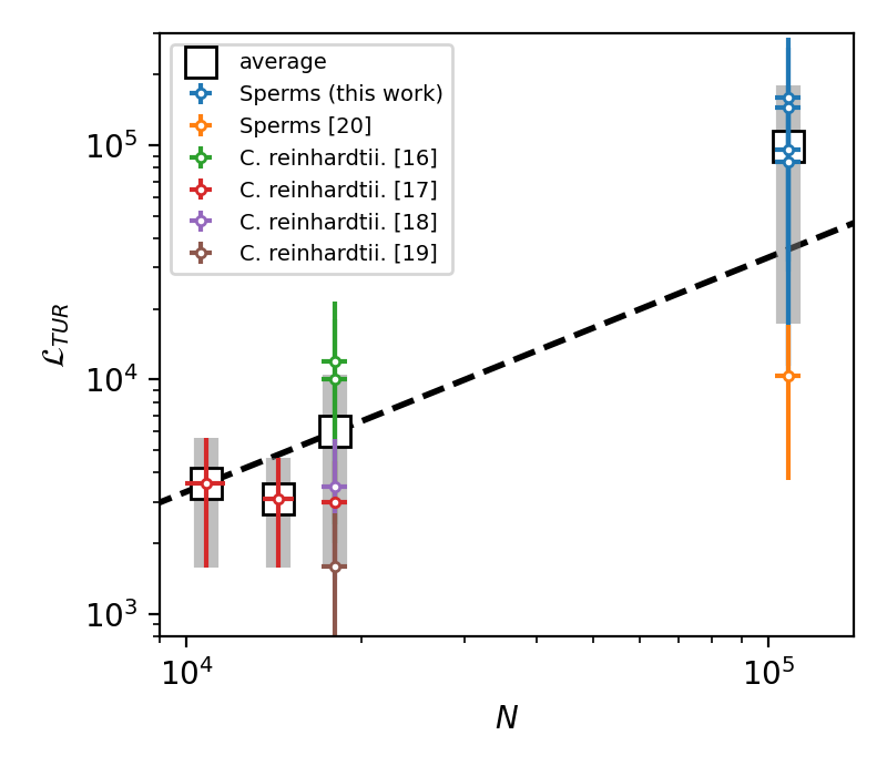
Figure 5: Collapse of correlation lengths in several experiments. The data from different previous experiments with sperms and flagella of C. reinhardtii algae are summarised here by plotting the correlation length $\mathcal{L}_{TUR}=\frac{\dot{W}}{pk_{B}T}$, discussed in the Appendix B.3, versus the length of the flagella $N$ (both quantities are given as numbers of molecular motors). The data are also reported in Table 1. The light colored points allow to distinguish the different experiments, while the solid circles identify the averages at each given flagellar length. Bars represent statistical errors. The dashed line marks the scaling law $\mathcal{L}_{TUR}\sim N$ which is expected under the hypothesis of strong coordination among adjacent motors in the axoneme.

We underline that, in order to extrapolate it to other systems and more general conditions, the identification with $N$ for the ratio between the TUR bound and the actual sperm precision should be taken as an order of magnitude. Here we discuss this point in closer details. We propose to generalise our observation to assemblies of $N$ molecular motors in the form $p_{max}\approx\dot{W}/(\mathcal{L}_{TUR}k_{B}T)$ where $\mathcal{L}_{TUR}\sim N$ is a correlation length (measured in adimensional units, i.e. as an estimate of the number of adjacent correlated motors). In the Appendix B.3 section we show that such a generalisation follows by considering a chain of molecular motors whose dynamics is correlated up to an extension of $\sim\mathcal{L}_{TUR}$ adjacent motors, leading to a renormalisation of the precision by a factor $\mathcal{L}_{TUR}$. In order to corroborate our conjecture, we reconsidered several previous results where the quality factor for fluctuations was measured in different conditions and with different flagella (from sperms and C. reinhardtii algae) Goldstein et al. (2009, 2011); Wan and Goldstein (2014); Quaranta et al. (2015); Ma et al. (2014). A summary of our and previous results is given in Table 1, in Appendix B.4. Our conjecture allows to collapse new and old data upon a master curve $\mathcal{L}_{TUR}\sim N$, fully consistent with our hypothesis, see Fig. 5.

VIII Conclusions and outlook

We have reported an experimental protocol to estimate the statistical precision of sperm’s beating, which differs from previous measurements of the quality factor as it is directly related to energy consumption, according to the recently celebrated TURs. The use of single-cell traps aids the reconstruction of the dynamics of a single cell’s shape, but in future implementations it could be replaced by a comoving tracking analysis directly applied upon free swimming cells.

Our results point to the need of understanding dynamical fluctuations of active flagella and their relation to their bioenergetics Skinner and Dunkel (2021); Yang et al. (2021); Tan et al. (2021). It seems that a recognised theoretical statement, the Thermodynamic Uncertainty Relation, has a relevance not only for molecular motors, but also for mesoscopic self-propelling microswimmers. With this aim, we have reported two striking observations: 1) the coincidence between the maximum precision of the whole sperm cell and that of molecular motors actuating the sperm’s flagellum, 2) the dependence of the maximum precision of the whole sperm cell upon the reduction of energy consumption, a dependence that one would expect only for the molecular motors. As a common explanation we conjecture that the $N\approx 10^{5}$ dynein motors actuating a sperm’s tail work at a high level of coordination which also affects fluctuations: a theoretical model where adjacent motors are coupled by a binding potential is consistent with out observations. The TUR is therefore still valid for the whole sperm’s cell, but with a discrepancy between maximum precision and energy consumption which is $\sim N$ times worse than in the case of the single molecular motor. An interesting perspective involves studying the same observables with other microswimmers, such as E. coli, whose flagellar motor fluctuations have been studied in the past Samuel and Berg (1995) but not their connection with the TUR. It will also be important to understand more deeply the detailed mechanical modelling of ciliary oscillations and how fluctuations can emerge from the dynamical instabilities that underlie the axonemal beating Riedel-Kruse et al. (2007); Sartori et al. (2016); Mondal et al. (2020). Validating such models will require a comparison with the full pdf of the beating phase fluctuations (and not only its extreme values).

We conclude emphasizing that our work suggests new applications of the TUR and of the precision observable. First, the TUR let us evaluate if the observed precision is low or not, as it gives a theoretical bound which can be reached by certain systems (for instance, some kinds of molecular motors get quite close to it). A large distance from such a bound is an observation which stimulates further investigation. Second, the precision $p$ helped us in validating the theoretical model: the scaling of $p$ with $N$ suggests the relevance of the coupling ingredient, beyond any precise calibration of the model parameters. Finally, $p$ could be made useful - in the future - in fertility studies and diagnostics, as it can enter the list of parameters measured in a spermiogram, to assess the health of human or animal sperm: for instance, our study suggests that it is correlated to the energy consumption of the cell. Of course the usefulness of such a parameter (e.g. if it is correlated with the good performance of a cell in chemotaxis, or other kinds of migration mechanisms) must be validated with further studies.

Appendix A: Experimental

Microfabrication

The micro-cage features allowed to accommodate one single cell on it, in a way that the head is confined while leaving the entire tail outside. Based on sperm characteristics, the chamber is designed as a box composed by four microfabricated facets anchored to the cover glass. The height, width and depth of a single cage are 500$\,nm$, 5.5$\,\mu m$ and 11$\,\mu m$, respectively. Microfabrication was carried out by a custom built two-photon polymerization setup Vizsnyiczai et al. (2017). The micro-chambers were generated from SU-8 3025 photoresist (Kayaku Advanced Materials) using a 60x 1.4NA objective. After exposure, the photoresist sample was baked ramping the temperature from 65 ^∘C up to 95 ^∘C with increments of 5 ^∘C per min, then 7 min at the highest temperature. Reduction of stress between the substrate and SU-8 is achieved by gradually decreasing the temperature of the sample until reaching room temperature. Thereafter, the photoresist was developed by its standard developer solvent, followed by rinsing in a 1:1 solution of water and ethanol, and finally dried with a gentle blow of nitrogen. Strong adhesion of the micro-chambers to the carrier cover glass was ensured by three layers of Omnicoat adhesion promoter (Kayaku Advanced Materials). Laser power and scanning speed were 5 mW and 30 $\mu ms^{-1}$, respectively.

Sample preparation

The experiments for measuring the main spatial modes of the sperm’s tail were developed on an open sample. This sample was obtained by attaching a plastic ring surrounding the micro-chambers area using the optical adhesive NOA81 (Norland Products Inc.). For the experiments under oxygen deprivation we used hermetically sealed samples. Two fishing wires of $\sim$100$\,\mu m$ thickness and NOA81 adhesive were used as spacers between the carrier cover glass and a cover slip, generating a channel; after introducing approximately 150$\,\mu L$ of solution containing sperm cells, the sample was completely sealed by applying NOA81 adhesive in the two open sides. Bull sperms were obtained from “Agrilinea S.R.L.” (Rome), and stored in a liquid nitrogen cylinder. On the day of the experiment, a vial of sperms suspended in semen was taken and immersed in a hot water bath of 37 degrees centigrade for 10 minutes. The vial was then taken out of the bath and immediately cut open using a pair of sterilized scissors. The sperm suspension was poured out of the vial in an Eppendorf. A micropipette was then used to suck out 150$\,\mu L$ of the sperm suspension from the Eppendorf and insert the fluid into the microchannel, ensuring proper filling inside the structures. The sperm movement was recorded at environmental temperature, $\sim 20^{\circ}C$, by using a digital camera (Nikon, USA) connected to an inverted microscope. The image capturing and analysis was performed using an in house software made using Python Programming language

Appendix B: Data Analysis

Details about the tail-tracking procedure

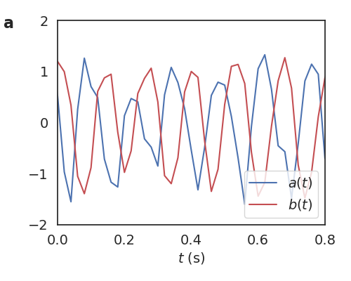
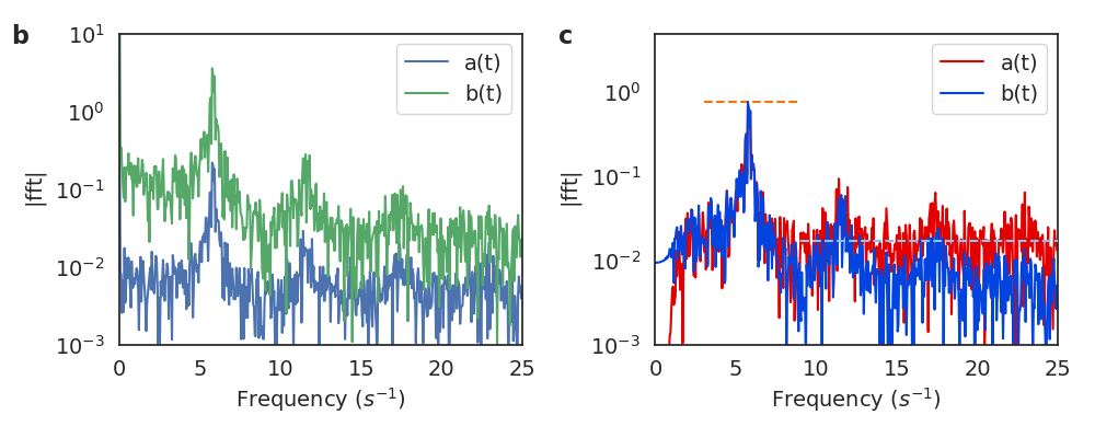
Figure 6: Details about the tail-tracking procedure. a, Examples of the signals $a(t)$ and $b(t)$ from trail tracking: one can see that $a(t)$ anticipates $b(t)$ of an angle between $\sim\pi/2$ and $\sim\pi$. b, spectra (modulus of the fast Fourier transform) of the signals $a(t)$ and $b(t)$. c, spectra after signal filtering. The orange and light-blue dashed lines indicate the signal level and the noise level respectively (the noise-to-signal ratio nsr is defined as the ratio between the latter and the former).

Images are collected at 50 frames per second, with 20x objective resulting in a resolution of $6.5/20$ $\mu m$ per pixel. Each image portrays a large portion of the substrate where several cages are present, almost all filled by caged sperms. Only cages with a single trapped sperm cell are analysed. A region of interest (ROI) of averagely $40\times 40$ pixels - corresponding to an area of roughly $13\times 13\mu m^{2}$ - containing the most visible part of the tail which is also the one closest to the head (see Fig. 1d), is cropped and treated by successive layers of image processing tools: 1) background subtraction to reduce noise, 2) transform to gradient (squared modulus) to avoid dependence on absolute levels, 3) Gaussian filter with $1$ pixel range, 4) the largest continuous bright region is individuated (it always corresponds to the tail), 5) that region is treated as a cloud of scattered points representing a curve $y$ vs. $x$, which is fitted by least squares to a second order polynomial $y(x,t)=a(t)+b(t)x+c(t)x^{2}$ as discussed in the main text. The time series of $a(t)$ and $b(t)$ are filtered by a $3$rd order Butterworth high-pass digital filter with critical frequency set $1.5$ Hz. In Figure 6 the time series of $a(t)$ and $b(t)$ of a tracked cell are shown, together with the spectra of the two series before and after the filtering. The noise-to-signal ratio (nsr) is computed as the ratio between the noise level and the signal level, both shown in the Figure.

Discussion of thermal diffusion effects due to the fluid

The value of $D$ is the result of a complex interplay of elasticity, hydrodynamics, activity and noises with different origins. Even at thermal equilibrium, i.e. for dead sperms, an estimate of filament phase diffusivity is complex as it involves not only the amplitude of fluctuations, that can be inferred by equilibrium distribution of elastic energy, but also the relaxation time of such modes. A first estimate of involved timescales can be obtained by computing the rotational diffusivity. For a passive rod Elgeti and Gompper (2009) (or a filament with low flexibility) of length $\ell\approx 50\mu m$ (as the sperm’s body) in water viscosity $\eta$ one has a rotational diffusivity of the order $D_{Stokes}\approx k_{B}T/(\eta\ell^{3})\approx 10^{-5}\textrm{rad}^{2}/s$. Visual inspection of our samples show that non-motile cells are basically immobile with negligible fluctuations in position or in shape, within our space-time resolution.

Correlation length based upon the thermodynamic uncertainty relation

Here we discuss a simple scaling argument to pinpoint the minimal assumptions behind the definition of an uncertainty correlation length

$$\mathcal{L}_{TUR}=\frac{\dot{W}}{p_{N}k_{B}T}$$ (5)

for a system of $N$ connected motors (e.g. a chain similar to the axoneme structure). We recall that the asymptotic (steady state) precision $p$ is defined as

$$p_{N}=\lim_{t\to\infty}\frac{1}{t}\frac{\langle X_{N}(t)\rangle^{2}}{\langle X_{N}^{2}\rangle_{c}}$$ (6)

where $\langle x^{2}\rangle_{c}$ stands for the variance of variable $x$, and $X_{N}(t)=\int_{0}^{t}ds\dot{X}_{N}(s)$ is the observed integrated current.

At a first order approximation, the presence of spatial correlations across a correlation length $\tilde{N}$ inside the chain can be accounted for by re-grouping the $N$ motors in $M=N/\tilde{N}$ independent groups. Moreover the observed integrated current $X_{N}$ can be assumed to be an empirical average of the integrated current in each of the $M$ independent groups, i.e.

$$X_{N}=\frac{\sum_{i=1}^{M}X_{\tilde{N},i}}{M},$$ (7)

with the $X_{\tilde{N},i}$ being independent and identically distributed. These assumptions lead to

$$p_{N}=\lim_{t\to\infty}\frac{1}{t}\frac{\langle X_{\tilde{N}}(t)\rangle^{2}}{\langle X_{\tilde{N}}^{2}\rangle_{c}/M}=Mp_{\tilde{N}}.$$ (8)

Assuming that the mean consumed work is extensive in the size of the chain, i.e. $\dot{W}_{N}\sim N\dot{W}_{1}$, we get

$$\frac{\dot{W}_{N}}{p_{N}k_{B}T}=\tilde{N}\frac{\dot{W}_{1}}{p_{\tilde{N}}}=(\mathcal{Q}_{micro})^{-1}\tilde{N},$$ (9)

having considered

$$\frac{\dot{W}_{1}}{p_{\tilde{N}}}\approx\frac{\dot{W}_{1}}{p_{1}}=(\mathcal{Q}_{micro})^{-1}$$ (10)

In the last passage we have assumed $p_{\tilde{N}}\approx p_{1}$ following the assumption that for the correlated $\tilde{N}$ motors in a group the precision is that of a single motor. Eq. (9) justifies our definition in Eq. (5)

Previous experiments with sperms at physiological temperature and with other flagella.

In a recent work Ma et al. (2014) data from sperm cells observed at 37 °C have been analysed. Such data, collected in a previous work Riedel-Kruse et al. (2007) concern an anomalous swimming regime which is apparently induced by a particular sample preparation: they were “incubated with 1% F-127 (Sigma) in PBS for 5 min…. When the surface was treated with F-127, the sperm did not stick but instead swam close to the surface, usually in circles of radii on the order of 40 $\mu m$” Riedel-Kruse et al. (2007). With such treatment the measured beating frequency was particularly high, we denote it as $f_{Ma}\sim 31$ Hz, much higher than what usually observed (literature reports $20$ Hz for bull sperm cells at 37 °C Rikmenspoel (1984), observed also in Riedel-Kruse et al. (2007) without such surface treatment). Within such particular conditions the authors measured a quality factor which, in our notation, reads $q=J/2D\sim 38$ that would correspond to a precision $p=2qJ$.

Other experimental works have addressed the properties of noise in the beating of axonemes, particularly with Chlamydomonas flagella Goldstein et al. (2009, 2011); Wan and Goldstein (2014); Polin et al. (2009); Quaranta et al. (2015) . In Goldstein et al. (2009, 2011) the quality factor of beating was obtained indirectly from the rate of phase slips in pairs of synchronised flagella (as well as directly from the distribution of beating periods), getting estimates in a range $q=25-120$, with average beating frequency $f=50Hz$.

A summary of such previous observations and a comparison with the results of the present study is given in Table 1. In compiling this table we have used some assumptions typically found in the literature i.e. that the amplitude of sperm’s beating is $6\pm 1\mu m$, the amplitude (”wingspan”) of Chlamydomonas flagellar beating is $10\pm 1\mu m$, and the energy consumption in both cases is given by Taylor formula Eq. (4) multiplied by $10$ (that is assuming an average efficiency of $10\%$).

Experiment	$f$	$L$	$N$	$\dot{W}/(k_{B}T)$	$q$	$p_{max}$	$\mathcal{L}_{TUR}$
Sperms (this study)	$8\pm 1$	$60\pm 3$	$1.1\cdot 10^{5}$	$10^{7}$	/	$120\pm 30$	$8.5\cdot 10^{4}$
Sperms after $\sim 2$ hours	$6\pm 1$	$60\pm 3$	$1.1\cdot 10^{5}$	$5.7\cdot 10^{6}$	/	$60\pm 10$	$9.6\cdot 10^{4}$
Sperm after $\sim 4$ hours	$3\pm 1$	$60\pm 3$	$1.1\cdot 10^{5}$	$1.4\cdot 10^{6}$	/	$10\pm 5$	$1.4\cdot 10^{5}$
Sperm after $\sim 5$ hours	$2\pm 1$	$60\pm 3$	$1.1\cdot 10^{5}$	$6.4\cdot 10^{5}$	/	$4\pm 0.5$	$1.6\cdot 10^{5}$
Sperms at 37 °C Ma et al. (2014)	$31\pm 1$	$60\pm 3$	$1.1\cdot 10^{5}$	$1.5\cdot 10^{8}$	$38\pm 5$	$1.4\cdot 10^{4}$	$10^{4}$
Chlamydomonas  Goldstein et al. (2009)	$47\pm 2$	$10\pm 0.5$	$1.8\cdot 10^{4}$	$1.6\cdot 10^{8}$	$23\pm 16$	$1.3\cdot 10^{4}$	$1.2\cdot 10^{4}$
Chlamydomonas  Goldstein et al. (2009)	$47\pm 2$	$10\pm 0.5$	$1.8\cdot 10^{4}$	$1.6\cdot 10^{8}$	$26\pm 18$	$1.6\cdot 10^{4}$	$10^{4}$
Chlamydomonas  Goldstein et al. (2011)	$71\pm 2$	$6\pm 0.5$	$10^{4}$	$2.3\cdot 10^{8}$	$70\pm 10$	$6.2\cdot 10^{4}$	$3.6\cdot 10^{3}$
Chlamydomonas  Goldstein et al. (2011)	$67\pm 2$	$8\pm 0.5$	$1.4\cdot 10^{4}$	$2.6\cdot 10^{8}$	$100\pm 12$	$8.3\cdot 10^{4}$	$3.1\cdot 10^{3}$
Chlamydomonas  Goldstein et al. (2011)	$62\pm 2$	$10\pm 0.5$	$1.8\cdot 10^{4}$	$2.9\cdot 10^{8}$	$120\pm 18$	$9.6\cdot 10^{4}$	$3\cdot 10^{3}$
Chlamydomonas  Wan and Goldstein (2014)	$60\pm 3$	$10\pm 0.5$	$1.8\cdot 10^{4}$	$2.7\cdot 10^{8}$	$100\pm 20$	$7.5\cdot 10^{4}$	$3.5\cdot 10^{3}$
Chlamydomonas  Quaranta et al. (2015)	$53\pm 2$	$10\pm 0.5$	$1.8\cdot 10^{4}$	$2\cdot 10^{8}$	$199\pm 20$	$1.3\cdot 10^{5}$	$1.6\cdot 10^{3}$

Table 1: Summary table of results from previous literature and from the present studies for both sperms and Chlamydomonas. The columns report the kind of experiment (with reference), the frequency of beating (in Hz), the length of the flagellum (in $\mu m$), the estimated number of motors $N=1800L$, the energy consumption in units of $k_{B}T$, the quality factor $q$ (when measured), the maximum observed precision $p_{max}$ (in $s^{-1}$) and the precision-based correlation length $\mathcal{L}_{TUR}=\dot{W}/(pk_{B}T)$ in number of motors, see Appendix B.3. For reasons of space we have not reported the errors if they can be computed by standard error propagation. The reported errors are those obtained from estimate reported in the literature and standard deviations in our experimental observations.

A plot of the TUR-based correlation length versus the length of the flagellum is shown in Figure 5. Within the error, the data are compatible with long-range order, i.e. $\mathcal{L}_{TUR}\sim N$.

Estimates of the energy consumption and efficiency of sperm swimming.

Consumption rate, speed and beating frequency are sensitive to environmental conditions, e.g. temperature and fluid viscosity Rikmenspoel (1984). In Brokaw (1967) sea urchin sperm was studied in a 50% glycerol solution at $16^{\circ}C$ with varying the beating frequencies through modulation of the ATP concentration: for instance at $20$ Hz it was found $10^{6}$ molecules of ATP per sperm per second, corresponding to slightly more than $\approx 10^{7}k_{B}T$ per second. In Rikmenspoel et al. (1969) experiments were performed at $37^{\circ}C$, with bull semen diluted/washed in egg yolk with diluents, a phosphate buffer and the addition of fructose and lactate, leading to an estimate of consumption rate equal to $\approx 10^{7}$ molecules of ATP per sperm per second, i.e. slightly more than $\approx 10^{8}k_{B}T$ per second. The evaluation of the produced work through the Taylor formula led to an estimate of the efficiency of $\sim 20\%$. In Chen et al. (2015) sea urchin sperms are studied one by one in droplet solutions, at unreported temperature but with controlled conditions in both ATP concentration and buffer viscosity (both directly modulating the beating frequency), obtaining $\sim 3\cdot 10^{6}$ ATP molecules per sperm per second when the tail beats at $10$ Hz.

Appendix C: A theoretical model for the fluctuations of an active axoneme

The model discussed in this section is a variation of the classical model introduced in Jülicher and Prost (1997) and further studied in Guérin et al. (2011a) and Guérin et al. (2011b).

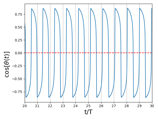
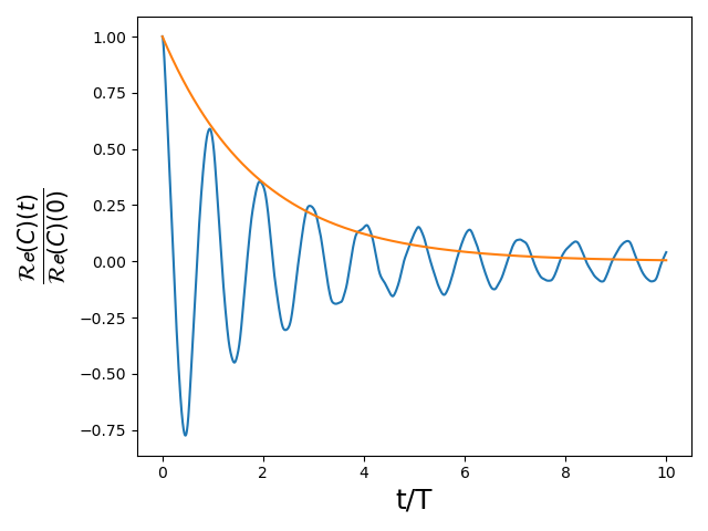
Figure 7: Theoretical model. a,d, evolution of the system in the force-coordinate phase space ($K=0$ in a and $K=10$ in d), the angle $\theta(t)$ measures the phase of this limit cycle after suitable rotation and normalisation of axis; b,e, evolution of $\cos[\theta(t)]$ that allows to evaluate the stability of the periods in the two cases ($K=0$ in b and $K=10$ in e); c,f: real part of the autocorrelation of $e^{i\theta(t)}$ and exponential fit $\sim e^{-Dt}$ of its envelope ($K=0$ in c and $K=10$ in f). In all the simulations we have used $\alpha=\eta=0.5$, $k/(\xi\Omega)=10$, $\alpha NU_{0}/(\Omega\ell^{2}\xi)=0.6$.

Interestingly the original model has been used to rationalise recent experiments on sperm swimming fluctuations Ma et al. (2014). In the original model however, the fluctuations of the $N$ motors are independent, therefore the fluctuations of the filament macroscopic dynamics are somehow similar to the fluctuations of an average of $N$ independent noises, therefore their squared error (or diffusivity) decreases with $N$ and this result in a linear $\sim N$ increase of the precision (or quality factor). We provide a simple mechanism to couple the noises of the motors and verify, in numerical simulations, that this ingredient is sufficient - at strong coupling - to change the size scaling from $O(N)$ to $O(1)$.

In the model the filament is represented by a position $X(t)$ and by a potential $W=\sum_{i=1}^{N}s_{i}U[x_{i}-X(t)]$ which regulates the interaction of the filament with $N$ motors, each one being at fixed position $x_{i}$ and in attachment state $s_{i}=0,1$ ($0$ when detached and $1$ when attached). The position $X(t)$ can be understood as the real position in space of the center of mass of the filament, as well as a generalised coordinate representing the shape of it. The potential may be related to local properties of the filament, such as the local curvature which depends upon the time $t$ through the coordinate $X(t)$. Each motor can detach and re-attach from/to the filament, changing its state $s_{i}$, according to a Poisson process that violates detailed balance, as it happens when ATP $\to$ ADP+P process is involved. The overdamped equation of motion of the filament is $\xi\dot{X}(t)=F_{ext}(t)+F(t)$ where $F(t)=-\partial_{X}\sum_{i}s_{i}U[x_{i}-X(t)]$ and $F_{ext}(t)$ is an external force. In general the filament can be free from external forces, but then a spatial asymmetry (employed in $W(x)$) is needed to induce forward motion, otherwise an external force (e.g. a spring on an end of the filament) is already sufficient to break spatial symmetry and the potential $W$ can be taken symmetric to simplify calculations. This is the case analysed here and in Ma et al. (2014), with $F_{ext}=-\kappa X$ and $U(x)=U_{0}[1-\cos(2\pi x/\ell)]$, the filament does not move on average but fluctuates more or less regularly, while a limit cycle in the plane $X(t),F(t)$ can be used as analogous to the $A,B$ plane used in our experiments. In the original model, each motor realises the attachment/detachment process independently from the other motors, with the only indirect correlations due to the modulation of the attachment/detachment rate through the position $\omega_{on}^{i}=\Omega[\eta-\alpha\cos(2\pi(x_{i}-X(t))/\ell)]$ and $\omega_{off}^{i}=\Omega-\omega_{on}^{i}$, . This ingredient however only correlates (locally) the average residence times but does not correlate fluctuations around those averages: it is the same as considering independent noises with similar averages.

In order to adapt the model to our experimental findings, we introduced a binding potential that correlates adjacent motors: this potential is minimised when adjacent motors are in the same state. This is implemented as a modification of the rates according to the formula $\omega_{on}^{i}=\Omega[\eta-\alpha\cos(2\pi(x_{i}-X(t))/\ell)]e^{-\Delta U^{bind}_{i}}$ and $\omega_{off}^{i}=\Omega-\Omega[\eta-\alpha\cos(2\pi(x_{i}-X(t))/\ell)]e^{-\Delta U^{bind}_{i}}$, with $\Delta U^{bind}_{i}$ is the binding potential increase after the variation of state $s_{i}$ of the $i$-th motor, and the binding potential is $U^{bind}_{i}=K(s_{i}-s_{i+1})^{2}+K(s_{i}-s_{i-1})^{2}$. When $K=0$ the original model without binding energy is recovered.

The effect of $K$ can be appreciated in numerical simulations of the model whose results are reported in Fig. 3 and 7. In particular in Figure 7c-f we show the drastic change in the decay of the phase correlation when $K$ is increased. In Fig. 3b it can be appreciated how the size scaling of the precision changes completely and tends to become independent of $N$ when the coupling strength increases. Our observation that the macroscopic sperm precision ($N\sim 10^{5}$) is similar to the microscopic sperm precision ($N=1$) is fairly explained by this new model. Note that the beating frequency in the model is independent of $N$ (at least for $N\gtrsim 10^{2}$) so that the energy consumption (ATP consumed per cycle and per motor) increases with $N$, even for large binding potential. The ratio between precision $p\sim O(1)$ and energy consumption $\dot{W}\sim N$ is therefore doomed to decrease as $1/N$, in fair agreement with experimental observations.

Appendix D: The simplest working principle for Thermodynamic Uncertainty Relations

While the TURs have been demonstrated for larger and larger classes of models and time domains, we judge instructive to summarise the first example where they have been observed which is a Markov jump process describing - in a very simplified way - the stochastic (progressive on average) dynamics of a single Brownian motor or clock Barato and Seifert (2015). The model is defined in continuous time, the motor can go forward or backward with probability rates $k_{+}$ and $k_{-}$ respectively. Local detailed balance dictates $k_{+}/k_{-}\sim\exp(Q/k_{B}T)$ where $Q=W$ is the energy dissipated in a forward jump equal to the work input carried by ATP.

The average current of the clock (number of steps per unit of time) is $J=k_{+}-k_{-}$, while the associated diffusivity is $2D=k_{+}+k_{-}$, therefore for the position $X(t)$ of the motor/clock one has a relative uncertainty defined as $\epsilon^{2}=(\langle X^{2}\rangle-\langle X\rangle^{2})^{2}/\langle X\rangle^{2}$ which reads $\epsilon^{2}=2Dt/(Jt)^{2}=(k_{+}+k_{-})/[(k_{+}-k_{-})^{2}t]$ which in terms of the precision $p=2/(t\epsilon^{2})$ reads $p=2(k_{+}-k_{-})^{2}/(k_{+}+k_{-})$. The energy dissipated up to time $t$ reads, in terms of the entropy production rate $\sigma$, $T\sigma t=\dot{Q}t=JQt$. Then the product between the energy dissipated and the relative uncertainty satisfies $2\dot{Q}/p=T\sigma t\epsilon^{2}=(k_{+}+k_{-})/(k_{+}-k_{-})Q\coth[Q/(2k_{B}T)]\geq 2k_{B}T$ which leads to the TUR used in this paper $p\leq\dot{Q}/(k_{B}T)$.

This example is useful to evaluate the key sources of noise in this process, i.e. the contributions to $D$ which are both $k_{+}$ and $k_{-}$. This means that backstepping (a not negligible $k_{-}$) is not the only source of noise, but $k_{+}$ also contributes to noise. The reason is that a large contribution to fluctuations of the motor current is due to fluctuations in the residence time before a new forward step. If time is discretized in $dt$ steps, the motor remains in its position with a probability $1-(k_{+})dt-(k_{-})dt$: the exit time has an exponential probability with average exit rate $(k_{+})+(k_{-})$. The real chemical network of a molecular motor, such as the dynein, is much richer than the minimal model considered in Barato and Seifert (2015); Howard (2001); Peliti and Pigolotti (2021): in that minimal model a single step is a coarse-graining of the several intermediate chemical steps. The presence of intermediate steps with their fluctuating residence of times and possibly non-negligible backstepping probabilities implies relevant fluctuations in the coarse-grained residence times and therefore in the motor’s current, even when the total back-stepping probability is negligible. We deem these motors’ fluctuations, with an additional coordination hypothesis discussed in the text, to be important for the deviation of the sperm shape cycle from its average dynamics.

SUPPLEMENTAL MATERIAL

Tracking the head oscillations

In a series of experiments we have tracked the sperm’s head instead of the tail, finding results in qualitative and quantitative agreement with those reported in the main article. The setup is identical, but different lighting and focus conditions with the microscope allowed us to have more image contrast in the interior of the cages. Images are collected with the same objective and ccd as in the main experiment. The region of interest is averagely the same area as in the main experiment. Background subtraction reduces the visibility of cage’s boundaries. The covariance matrix of the pixel light distribution is computed: its eigenvector associated to the maximum eigenvalue determines the direction of orientation of the sperm’s head, whose slope replaces coefficient $-b(t)$ of our tail’s analysis (the minus sign of course depends upon the reference frame we are using). The $\hat{y}$ position of the center of mass of the head replaces coefficient $a(t)$. Once we get $a(t),b(t)$ for the image at time $t$ we can repeat exactly the same analysis as we did for the tail’s tracking. In Figure S1 we summarise the results of this analysis.

Fig. S1 Head tracking. a, Example of a head tracking where $a(t)$ and $b(t)$ (bottom plot) are obtained by computing the height ($y$ position in the region of interest) of the center of mass of the pixel distribution and the slope of the direction associated with the maximum eigenvalue of the pixel covariance matrix. b, spectra of the signals $a(t)$ and $b(t)$. c, spectra after signal filtering. The orange and light-blue dashed lines indicate the signal level and the noise level respectively. d, Examples of the signals $a(t)$ and $b(t)$ from head tracking: again $a(t)$ anticipates $b(t)$ of an angle between $\sim\pi$ and $\sim\pi/2$. e, Integrated phase-space current $\theta(t)$ for a few observed sperms. f, Pdf (over $20$ seconds acquisition), for a few sperms, of $\delta\theta=\theta(t+dt)-\theta(t)$ (shifted by the mean and scaled by the standard deviation), where $dt=0.02$ seconds. g, Precision $p$ versus the noise-to-signal ratio (nsr) computed from the signals $a(t)$ and $b(t)$. The sample size consists of $58$ different observed sperm cells.

Alternative estimates of the precision

In a recent paper the fluctuations of the sperm beating cycle have been analysed Ma et al. (2014). The Authors suggest two alternative ways to estimate the phase diffusivity $D$ which is necessary to get values for $p=J^{2}/D$ (being $J=2\pi f$ and $f$ the average beating frequency). A first, perhaps more approximate, procedure is to retrieve the quality factor $q=f_{0}/\Delta f_{0}$ where $\Delta f_{0}$ is the width-at-half-maximum in the power spectrum, which reads $\Delta f_{0}\sim 3$ Hz giving $q\approx 3$. The quality factor is related to the phase diffusivity by $q=J/(2D)$ which leads to $p=J^{2}/D=2Jq\approx 2\times 10^{2}s^{-1}$ which is compatible in order of magnitude with the maximum precision we report in the main text. The second recipe consists in measuring the decay in time of the phase correlation $C(t)=\langle\exp i[\theta(t_{0}+t)-\theta(t_{0})]\rangle\sim e^{-Dt}$, as we have also done for the simulations of the theoretical model in the Main text. Examples of the decay of $C(t)$ are shown in Figure S2. The obtained values of $D$ lead to a precision of the order of $p_{max}\sim 5\times 10^{2}s^{-1}$ and smaller by a factor $\sim 10$ after $5$ hours of oxygen deprivation, in full agreement with the results shown in the Main text.

Fig. S2 Phase correlation decay for three different sperms in experiments. The first two are at the starting time of the experiment, while the third is after $150$ minutes. The precisions measured are $\sim 500s^{-1}$, $\sim 400s^{-1}$ and $\sim 80s^{-1}$.

$\theta$	integrated current (beating phase)
$J$	average current
${\textrm{m}sd}$	mean squared displacement of $\theta$
$D$	diffusivity of $\theta$
$p$	precision
$p_{max}$	estimate of the largest precision in the sperm’s population
$p_{TUR}$	theoretical bound for the precision, based upon the TUR
$\dot{W}$	energy consumption rate
$T$	temperature
$k_{B}$	Boltzmann’s constant
nsr	noise to signal ratio
$\eta$	fluid viscosity
$L$	length of the flagellum
$f$	beating frequency
$\beta$	beating amplitude
$\mathcal{Q}$	TUR-based figure of merit, i.e. $p_{max}/p_{TUR}$
$\mathcal{Q}_{macro}$	TUR-based figure of merit for the whole flagellum or large chain of motors
$\mathcal{Q}_{micro}$	TUR-based figure of merit for the single motor
$X$	relative position between motors and flagellum in the theoretical model
$\xi$	viscous damping in the theoretical model
$\kappa$	elastic constant in the theoretical model
$s_{i}$	state variable ($0$ detached, $1$ attached) for the $i$-th motor in the theoretical model
$U(x)$	potential energy in the theoretical model
$N$	number of motors in the experiments (estimate) or in the theoretical model
$K$	coupling constant for the binding potential that couples the state of two adjacent motors
$\mathcal{L}_{TUR}$	putative correlation length defined according to the TUR
$k_{+},k_{-}$	probability rates for transitions in the simple motor model in Appendix D
$\epsilon$	relative uncertainty in the simple motor model in Appendix D
$\sigma$	entropy production rate in the simple motor model in Appendix D
$Q$	dissipated heat per cycle (equal to work input per cycle) in Appendix D
$q$	quality factor $q=J/(2D)=p/(2J)$

Table 2: List of symbols used in the text

References

- Lauga and Powers (2009) Eric Lauga and Thomas R Powers, “The hydrodynamics of swimming microorganisms,” Reports on Progress in Physics 72, 096601 (2009).
- Elgeti et al. (2015) Jens Elgeti, Roland G Winkler, and Gerhard Gompper, “Physics of microswimmers—single particle motion and collective behavior: a review,” Reports on Progress in Physics 78, 056601 (2015).
- Fauci and Dillon (2006) Lisa J Fauci and Robert Dillon, “Biofluidmechanics of reproduction,” Annual Review of Fluid Mechanics 38, 371–394 (2006).
- Tsang et al. (2020) Alan CH Tsang, Ebru Demir, Yang Ding, and On Shun Pak, “Roads to smart artificial microswimmers,” Advanced Intelligent Systems 2, 1900137 (2020).
- Lindemann and Lesich (2016) Charles B Lindemann and Kathleen A Lesich, “Functional anatomy of the mammalian sperm flagellum,” Cytoskeleton 73, 652–669 (2016).
- Machin (1958) KE Machin, “Wave propagation along flagella,” Journal of Experimental Biology 35, 796–806 (1958).
- Elgeti et al. (2010) Jens Elgeti, U Benjamin Kaupp, and Gerhard Gompper, “Hydrodynamics of sperm cells near surfaces,” Biophysical Journal 99, 1018–1026 (2010).
- Gaffney et al. (2011) Eamonn A Gaffney, Hermes Gadêlha, David J Smith, John R Blake, and Jackson C Kirkman-Brown, “Mammalian sperm motility: observation and theory,” Annual Review of Fluid Mechanics 43, 501–528 (2011).
- Crenshaw (1989) Hugh C Crenshaw, “Kinematics of helical motion of microorganisms capable of motion with four degrees of freedom,” Biophysical journal 56, 1029–1035 (1989).
- Gray and Hancock (1955) James Gray and GJ Hancock, “The propulsion of sea-urchin spermatozoa,” Journal of Experimental Biology 32, 802–814 (1955).
- Purcell (1977) Edward M Purcell, “Life at low reynolds number,” American Journal of Physics 45, 3–11 (1977).
- Jülicher and Prost (1997) Frank Jülicher and Jacques Prost, “Spontaneous oscillations of collective molecular motors,” Physical review letters 78, 4510 (1997).
- Friedrich and Jülicher (2008) BM Friedrich and F Jülicher, “The stochastic dance of circling sperm cells: sperm chemotaxis in the plane,” New Journal of Physics 10, 123025 (2008).
- Friedrich and Jülicher (2009) Benjamin M Friedrich and Frank Jülicher, “Steering chiral swimmers along noisy helical paths,” Physical Review Letters 103, 068102 (2009).
- Polin et al. (2009) Marco Polin, Idan Tuval, Knut Drescher, Jerry P Gollub, and Raymond E Goldstein, “Chlamydomonas swims with two “gears” in a eukaryotic version of run-and-tumble locomotion,” Science 325, 487–490 (2009).
- Goldstein et al. (2009) Raymond E Goldstein, Marco Polin, and Idan Tuval, “Noise and synchronization in pairs of beating eukaryotic flagella,” Physical review letters 103, 168103 (2009).
- Goldstein et al. (2011) Raymond E Goldstein, Marco Polin, and Idan Tuval, “Emergence of synchronized beating during the regrowth of eukaryotic flagella,” Physical Review Letters 107, 148103 (2011).
- Wan and Goldstein (2014) Kirsty Y Wan and Raymond E Goldstein, “Rhythmicity, recurrence, and recovery of flagellar beating,” Physical review letters 113, 238103 (2014).
- Quaranta et al. (2015) Greta Quaranta, Marie-Eve Aubin-Tam, and Daniel Tam, “Hydrodynamics versus intracellular coupling in the synchronization of eukaryotic flagella,” Physical review letters 115, 238101 (2015).
- Ma et al. (2014) Rui Ma, Gary S Klindt, Ingmar H Riedel-Kruse, Frank Jülicher, and Benjamin M Friedrich, “Active phase and amplitude fluctuations of flagellar beating,” Physical review letters 113, 048101 (2014).
- Klindt and Friedrich (2015) Gary S Klindt and Benjamin M Friedrich, “Flagellar swimmers oscillate between pusher-and puller-type swimming,” Physical Review E 92, 063019 (2015).
- Solovev and Friedrich (2022) Anton Solovev and Benjamin M Friedrich, “Synchronization in cilia carpets and the kuramoto model with local coupling: Breakup of global synchronization in the presence of noise,” Chaos: An Interdisciplinary Journal of Nonlinear Science 32, 013124 (2022).
- Barato and Seifert (2015) Andre C Barato and Udo Seifert, “Thermodynamic uncertainty relation for biomolecular processes,” Physical Review Letters 114, 158101 (2015).
- Gingrich et al. (2016) Todd R Gingrich, Jordan M Horowitz, Nikolay Perunov, and Jeremy L England, “Dissipation bounds all steady-state current fluctuations,” Physical Review Letters 116, 120601 (2016).
- Horowitz and Gingrich (2020) Jordan M Horowitz and Todd R Gingrich, “Thermodynamic uncertainty relations constrain non-equilibrium fluctuations,” Nature Physics 16, 15–20 (2020).
- Lindemann (2003) Charles B Lindemann, “Structural-functional relationships of the dynein, spokes, and central-pair projections predicted from an analysis of the forces acting within a flagellum,” Biophysical Journal 84, 4115–4126 (2003).
- Chen et al. (2015) Daniel TN Chen, Michael Heymann, Seth Fraden, Daniela Nicastro, and Zvonimir Dogic, “Atp consumption of eukaryotic flagella measured at a single-cell level,” Biophysical journal 109, 2562–2573 (2015).
- Gilpin et al. (2020) William Gilpin, Matthew Storm Bull, and Manu Prakash, “The multiscale physics of cilia and flagella,” Nature Reviews Physics 2, 74–88 (2020).
- Bustamante et al. (2001) Carlos Bustamante, David Keller, and George Oster, “The physics of molecular motors,” Accounts of Chemical Research 34, 412–420 (2001).
- Brokaw (2009) Charles J Brokaw, “Thinking about flagellar oscillation,” Cell Motility and the Cytoskeleton 66, 425–436 (2009).
- Brokaw (2002) Charles J Brokaw, “Computer simulation of flagellar movement viii: coordination of dynein by local curvature control can generate helical bending waves,” Cell motility and the cytoskeleton 53, 103–124 (2002).
- Burgess (1995) SA Burgess, “Rigor and relaxed outer dynein arms in replicas of cryofixed motile flagella,” Journal of molecular biology 250, 52–63 (1995).
- Goodenough and Heuser (1982) Ursula W Goodenough and John E Heuser, “Substructure of the outer dynein arm.” The Journal of cell biology 95, 798–815 (1982).
- Hwang and Hyeon (2018) Wonseok Hwang and Changbong Hyeon, “Energetic costs, precision, and transport efficiency of molecular motors,” The Journal of Physical Chemistry Letters 9, 513–520 (2018).
- Falasco and Esposito (2020) Gianmaria Falasco and Massimiliano Esposito, “Dissipation-time uncertainty relation,” Physical Review Letters 125, 120604 (2020).
- Rikmenspoel et al. (1960) R Rikmenspoel, G Van Herpen, and P Eijkhout, “Cinematographic observations of the movements of bull sperm cells,” Physics in Medicine & Biology 5, 167 (1960).
- Woolley (2003) DM Woolley, “Motility of spermatozoa at surfaces,” Reproduction 126, 259–270 (2003).
- Nosrati et al. (2015) Reza Nosrati, Amine Driouchi, Christopher M Yip, and David Sinton, “Two-dimensional slither swimming of sperm within a micrometre of a surface,” Nature Communications 6, 1–9 (2015).
- Saggiorato et al. (2017) Guglielmo Saggiorato, Luis Alvarez, Jan F Jikeli, U Benjamin Kaupp, Gerhard Gompper, and Jens Elgeti, “Human sperm steer with second harmonics of the flagellar beat,” Nature Communications 8, 1–9 (2017).
- (40) See Supplemental Material at [URL will be inserted by publisher] for the results of head oscillation tracking, a discussion of alternative estimates of the precision, a table of symbols used in the paper and a video with a caged sperm cell, its digitally tracked tail, recorded at six different time delays with respect to the starting time of the oxygen deprivation experiment.
- Battle et al. (2016) Christopher Battle, Chase P Broedersz, Nikta Fakhri, Veikko F Geyer, Jonathon Howard, Christoph F Schmidt, and Fred C MacKintosh, “Broken detailed balance at mesoscopic scales in active biological systems,” Science 352, 604–607 (2016).
- Gladrow et al. (2017) Jannes Gladrow, Chase P Broedersz, and Christoph F Schmidt, “Nonequilibrium dynamics of probe filaments in actin-myosin networks,” Physical Review E 96, 022408 (2017).
- Stephens et al. (2008) Greg J Stephens, Bethany Johnson-Kerner, William Bialek, and William S Ryu, “Dimensionality and dynamics in the behavior of c. elegans,” PLoS Computational Biology 4, e1000028 (2008).
- Gnesotto et al. (2018) FS Gnesotto, Federica Mura, Jannes Gladrow, and Chase P Broedersz, “Broken detailed balance and non-equilibrium dynamics in living systems: a review,” Reports on Progress in Physics 81, 066601 (2018).
- Li et al. (2019) Junang Li, Jordan M Horowitz, Todd R Gingrich, and Nikta Fakhri, “Quantifying dissipation using fluctuating currents,” Nature Communications 10, 1–9 (2019).
- Roldán et al. (2021) Édgar Roldán, Jérémie Barral, Pascal Martin, Juan MR Parrondo, and Frank Jülicher, “Quantifying entropy production in active fluctuations of the hair-cell bundle from time irreversibility and uncertainty relations,” New Journal of Physics 23, 083013 (2021).
- Brokaw (1967) CJ Brokaw, “Adenosine triphosphate usage by flagella,” Science 156, 76–78 (1967).
- Rikmenspoel et al. (1969) Robert Rikmenspoel, Sandra Sinton, and John J Janick, “Energy conversion in bull sperm flagella,” The Journal of General Physiology 54, 782–805 (1969).
- Rikmenspoel (1984) ROBERT Rikmenspoel, “Movements and active moments of bull sperm flagella as a function of temperature and viscosity,” Journal of Experimental Biology 108, 205–230 (1984).
- Brokaw (1966) CJ Brokaw, “Effects of increased viscosity on the movements of some invertebrate spermatozoa,” Journal of Experimental Biology 45, 113–139 (1966).
- Brokaw (1975) CJ Brokaw, “Effects of viscosity and atp concentration on the movement of reactivated sea-urchin sperm flagella,” Journal of Experimental Biology 62, 701–719 (1975).
- Nicastro et al. (2006) Daniela Nicastro, Cindi Schwartz, Jason Pierson, Richard Gaudette, Mary E Porter, and J Richard McIntosh, “The molecular architecture of axonemes revealed by cryoelectron tomography,” Science 313, 944–948 (2006).
- Carvalho-Santos et al. (2011) Zita Carvalho-Santos, Juliette Azimzadeh, José B Pereira-Leal, and Mónica Bettencourt-Dias, “Evolution: Tracing the origins of centrioles, cilia, and flagella,” The Journal of cell biology 194, 165 (2011).
- Klindt et al. (2016) Gary S Klindt, Christian Ruloff, Christian Wagner, and Benjamin M Friedrich, “Load response of the flagellar beat,” Physical review letters 117, 258101 (2016).
- Pellicciotta et al. (2020) Nicola Pellicciotta, Evelyn Hamilton, Jurij Kotar, Marion Faucourt, Nathalie Delgehyr, Nathalie Spassky, and Pietro Cicuta, “Entrainment of mammalian motile cilia in the brain with hydrodynamic forces,” Proceedings of the National Academy of Sciences 117, 8315–8325 (2020).
- Note (1) We remark that in this paper Hwang and Hyeon (2018) cytoplasmic dynein is considered, which is known to be structurally similar to the axonemal one, with also a few distinct features kato2014structure.
- Guérin et al. (2011a) Thomas Guérin, J Prost, and J-F Joanny, “Dynamical behavior of molecular motor assemblies in the rigid and crossbridge models,” The European Physical Journal E 34, 1–21 (2011a).
- Guérin et al. (2011b) T Guérin, J Prost, and J-F Joanny, “Bidirectional motion of motor assemblies and the weak-noise escape problem,” Physical Review E 84, 041901 (2011b).
- Skinner and Dunkel (2021) Dominic J Skinner and Jörn Dunkel, “Improved bounds on entropy production in living systems,” Proceedings of the National Academy of Sciences 118 (2021).
- Yang et al. (2021) Xingbo Yang, Matthias Heinemann, Jonathon Howard, Greg Huber, Srividya Iyer-Biswas, Guillaume Le Treut, Michael Lynch, Kristi L Montooth, Daniel J Needleman, Simone Pigolotti, et al., “Physical bioenergetics: Energy fluxes, budgets, and constraints in cells,” Proceedings of the National Academy of Sciences 118 (2021).
- Tan et al. (2021) Tzer Han Tan, Garrett A Watson, Yu-Chen Chao, Junang Li, Todd R Gingrich, Jordan M Horowitz, and Nikta Fakhri, “Scale-dependent irreversibility in living matter,” arXiv preprint arXiv:2107.05701 (2021).
- Samuel and Berg (1995) AD Samuel and Howard C Berg, “Fluctuation analysis of rotational speeds of the bacterial flagellar motor.” Proceedings of the National Academy of Sciences 92, 3502–3506 (1995).
- Riedel-Kruse et al. (2007) Ingmar H Riedel-Kruse, Andreas Hilfinger, Jonathon Howard, and Frank Jülicher, “How molecular motors shape the flagellar beat,” HFSP journal 1, 192–208 (2007).
- Sartori et al. (2016) Pablo Sartori, Veikko F Geyer, Andre Scholich, Frank Jülicher, and Jonathon Howard, “Dynamic curvature regulation accounts for the symmetric and asymmetric beats of chlamydomonas flagella,” Elife 5, e13258 (2016).
- Mondal et al. (2020) Debasmita Mondal, Ronojoy Adhikari, and Prerna Sharma, “Internal friction controls active ciliary oscillations near the instability threshold,” Science advances 6, eabb0503 (2020).
- Vizsnyiczai et al. (2017) Gaszton Vizsnyiczai, Giacomo Frangipane, Claudio Maggi, Filippo Saglimbeni, Silvio Bianchi, and Roberto Di Leonardo, “Light controlled 3d micromotors powered by bacteria,” Nature Communications 8, 15974 (2017).
- Elgeti and Gompper (2009) Jens Elgeti and Gerhard Gompper, “Self-propelled rods near surfaces,” EPL (Europhysics Letters) 85, 38002 (2009).
- Howard (2001) Jonathon Howard, Mechanics of Motor Proteins and the Cytoskeleton (Sinauer Associates Inc, 2001).
- Peliti and Pigolotti (2021) Luca Peliti and Simone Pigolotti, Stochastic Thermodynamics: An Introduction (Princeton University Press, 2021).