Supervised Fine-tuning Evaluation for Long-term Visual Place Recognition

Abstract

In this paper, we present a comprehensive study on the utility of deep convolutional neural networks with two state-of-the-art pooling layers which are placed after convolutional layers and fine-tuned in an end-to-end manner for visual place recognition task in challenging conditions, including seasonal and illumination variations. We compared extensively the performance of deep learned global features with three different loss functions, e.g. triplet, contrastive and ArcFace, for learning the parameters of the architectures in terms of fraction of the correct matches during deployment. To verify effectiveness of our results, we utilized two real world datasets in place recognition, both indoor and outdoor. Our investigation demonstrates that fine tuning architectures with ArcFace loss in an end-to-end manner outperforms other two losses by approximately $1\sim 4\;\%$ in outdoor and $1\sim 2\;\%$ in indoor datasets, given certain thresholds, for the visual place recognition tasks.

I Introduction

Image retrieval is a problem of searching for a query image in a large image database given the visual content of an image. Large-scale Visual Place Recognition (VPR) is commonly formulated as a subcategory of image retrieval problem to identify images which belong to similar places with same positions in robotics and autonomous systems [1]. It can generally be extended to broader areas, including topological mapping, loop closure and drift removal in geometric mapping and learning scene dynamics for long-term localization and mapping. Long-term operations in environments can cause significant image variations including illumination changes, occlusion and scene dynamics [2].

The recognition robustness of VPR systems depends on whether or not the matched images are taken at the same places in the real world given a certain threshold. Therefore, the retrieval performance is highly correlated with feature representation and similarity measurement [3]. One of the crucial challenges is to extract meaningful information of raw images in order to mitigate the semantic gap of low level image representation perceived by machines and high level semantic concept perceived by human [4].

Global feature descriptors are commonly utilized to obtain high image retrieval performance with compact image representations. Before deep learning era in computer vision, they were mainly developed by aggregating hand-crafted local descriptors. Deep Convolutional Neural Networks (DCNNs) are now the core of the most state-of-the-art computer vision techniques in wide variety of tasks, including image classification, object detection and image segmentation [5].

Recent advances of the generic descriptors extracted from DCNNs can learn discriminatory and human-level representation to provide high-level visual content of the image patterns [6]. These architectures can potentially learn features at multiple abstraction levels to map large raw sensory input data to the output, without relying on human-crafted features [7]. The DCNN-based global features are high performing descriptors trained with ranking-based or classification losses [8].

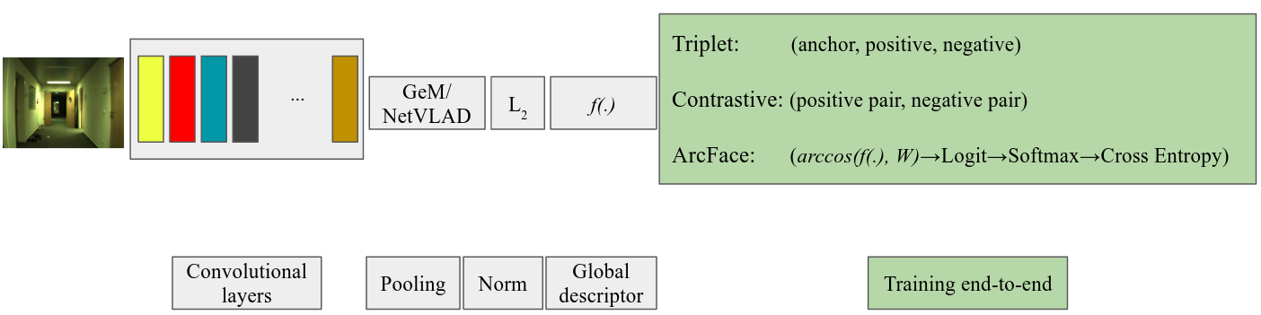
Figure 1: The architecture of our DCNN with the triplet, contrastive and ArcFace losses used for end-to-end training. A single vector global descriptor $f(.)$ is extracted to represent an image.

Throughout the past few years, several DCNNs have been designed to address image classification and objection detection. In this paper, our contribution is to conduct an all-embracing study on supervised fine-tuning of such DCNNs with two state-of-the-art pooling layers with learnable parameters, one for image retreival, i.e., GeM, and one for place recognition, i.e., NetVLAD, in an end-to-end manner for the VPR task on real world datasets. In our investigation, we report and analyze the performance of deep learned global features which are trained with three different loss functions in terms of the fraction of correct matches of query images compared to the reference images.

The rest of this paper is organized as follows. Section II briefly discusses the related work. In section III, we provide the baseline methods along with section IV which explains two real-world indoor and outdoor datasets to address the VPR task. In section V, we show the experimental results and we conclude the paper in section VI.

II Related Work

Before the rise and dominance of DCNNs, VPR methods utilized conventional hand-crafted features such as local and global image descriptors, to match query images with the reference database [9, 10, 11]. However, deep features have shown more robust performance than handcrafted features to address the geometric transformations and illumination changes.

DCNN-based VPR methods can be divided into two main categories. 1) Methods with pre-trained DCNN models, utilized as feature extractor to construct image representation to measure the image similarity. 2) Methods with fine-tune models on specific VPR datasets or new architecture to improve the recognition performance.

Chen et al. [12] introduced the first off-the-shelf DCNN-based VPR system with features extracted from a pre-trained Overfeat [13] model in challenging conditions. Sünderhauf et al. [14] evaluated the intermediate conv3 layer of AlexNet, primarily trained for image classification, as holistic image representation to match places across condition changes between query and reference database. Chen et al. [15] trained AmosNet and HybridNet on a large-scale dataset to address the appearance and viewpoint variations. Lopez et al. [16] fine-tuned AlexNet pre-trained architecture on ImageNet dataset for VPR with triplets of images containing original image stacked with similar and dissimilar pairs. Feature post-processing methods, e.g., feature augmentation and standardization have shown improvement compared to using raw holistic DCNN-descriptors [17, 18, 19].

DCNN-based VPR methods can learn robust feature mapping to enable image comparison using similarity measures such as Euclidean distance. Single feedforward pass methods take the whole image as an input followed by pooling or aggregation on the raw features to design more global discriminative features in which the whole image is described by as single feature vector, i.e., global descriptor.

A number of architectures have been proposed to address the image representation with global descriptor: MAC [20], SPoC [21], CroW [22], GeM [23], R-MAC [24], modified R-MAC [25]. Moreover, there are DCNNs especially trained for VPR to retreive either global image descriptors, e.g., NetVLAD [26] or local features, e.g., DELF [27].

In this paper, we selected and fine-tuned two state-of-the-art methods for global descriptors, e.g., GeM and NetVLAD which are trained in an end-to-end manner for both indoor and outdoor VPR datasets.

III Baseline Methods

III-A Pooling Layer

Adding pooling layer after the convolutional layer is a common pattern for layer ordering of DCNNs to create a new set of the same number of pooled feature maps. In what follows, we provide a brief summary of GeM and NetVLAD pooling layers, utilized as pooling layers in this paper:

GeM

Radenović et al. [28, 23] adopt the siamese architecture for training. It is trained using positive and negative image pairs and the loss function enforces large distances between negative pairs, e.g., images from two distant places and small distances between positive pairs, e.g., images from the same place. Feature vectors are global descriptors of the input images and pooled over the spatial dimensions. The feature responses are computed from $K$ convolutional layers $\mathcal{X}_{k}$ following with max pooling layers that select the maximum spatial feature response from each layer of MAC:

$$\vec{f}=\left[f_{1}~{}f_{2}~{}\ldots~{}f_{K}\right],~{}f_{k}=\max_{x\in\mathcal{X}_{k}}x\enspace.$$ (1)

GeM pooling layer is proposed to modify MAC [20] and SPoC [21] for better performance. This is a pooling layer which takes $\chi$ as an input and produces a vector $f=[f_{1},f_{2},f_{i},...,f_{K}]^{T}$ as an output of the pooling process which results in:

$$f_{i}=\left(\frac{1}{|\chi_{i}|}\sum_{x\in\chi_{i}}x^{p_{i}}\right)^{\frac{1}{p_{i}}}$$ (2)

MAC and SPoC are special cases of GeM pooling layer depending on how pooling parameter $p_{k}$ is derived in which $p_{i}\rightarrow\infty$ and $p_{i}=1$ correspond to max-pooling and average pooling, respectively. The GeM feature vector is a single value per feature map and its dimension varies depending on different networks, i.e. $K=[256,\;512,\;2048]$.

NetVLAD

Function $f$ is defined as the global feature vector for a given image $I$ as $f(I)$. This function is used to extract the feature vectors from the entire reference database ${I_{i}}$. Then visual search between $f(q)$, e.g., query image and the reference images $f(I_{i})$ is performed using Euclidean distance $d(q,I_{i})$ and by selecting the top-N matches. NetVLAD is inspired by the conventional VLAD [11] which uses handcrafted SIFT descriptors [29] and uses VLAD encoding to form $f(I)$.

To learn the representation end-to-end, NetVLAD contains two main building blocks. 1) Cropped CNN at the last convolutional layer, identified as a dense descriptor with the output size of $H\times W\times D$, correspond to set of $D$-dimensional descriptors extracted at $H\times W$ spatial locations. 2) Trainable generalized VLAD layer, e.g., Netvlad which pools extracted descriptors into a fixed image representation in which its parameters trained via backpropagation.

The original VLAD image representation $V$ is $D\times K$ matrix in which $D$ is the dimension of the input local image descriptor ${\vec{x}_{i}}$ and $K$ is the number of clusters. It is reshaped in to a vector after $L_{2}$-normalization and $(j,k)$ element of $V$ is calculated as follows:

$$V(j,k)=\sum_{i=1}^{N}a_{k}(\vec{x}_{i})(x_{i}(j)-c_{k}(j)),$$ (3)

where $x_{i}(j)$ and $c_{k}(j)$ are the $j$th dimensions of the $i$th descriptor and $k$th cluster centers, respectively. $a_{k}(\vec{x}_{i})=0,1$ indicates whether or not descriptor $\vec{x}_{i}$ belongs to $k$th visual word. Compared to original VLAD, Netvlad layer is differentiable thanks to its soft assignment of descriptors to multiple clusters:

$$V(j,k)=\sum_{i=1}^{N}\frac{e^{w_{k}^{T}x_{i}+b_{k}}}{\sum_{k^{\prime}}e^{w_{k^{\prime}}^{T}x_{i}+b_{k^{\prime}}}}(x_{i}(j)-c_{k^{\prime}}(j))$$ (4)

where ${w_{k}}$, ${b_{k}}$ and ${c_{k}}$ are gradient descent optimized parameters of $k$ clusters.

In our experiments with 64 clusters and $512$-dimensional VGG16 backbone, the NetVLAD feature vector dimension becomes $512\times 64=32,768$. Arandjelovic et al. [26] used PCA dimensionality reduction method as a post-processing stage. However, in our experiment we utilized full size of feature vector. Since NetVLAD layer can be easily plugged into any other CNN architecture in an end-to-end manner, we investigate its performance with VGG16 and ResNet50 backbones and report the results in section V.

III-B Loss Function

One of the main challenges of feature learning in large-scale DCNN-based VPR methods is to design an appropriate loss function to improve the the discriminative power and recognition ability [30]. We evaluated the loss functions for the VPR task in two categories. 1) Measure the difference between samples based on the Euclidean space distance, e.g., contrastive loss and triplet loss. 2) Measure the difference between samples based on angular space, e.g., ArcFace loss.

Contrastive

Given the siamese architecture, the training input consists of image pairs $(a,b)$ and labels $y(a,b)=\{0,1\}$ declaring whether a pair is non-matching ($y=0$) or matching ($y=1$). Contrastive loss [31] acts on matching (positive) and non-matching (negative) pairs as follows:

$$\mathcal{L_{C}}=\begin{cases}{l}(\vec{f}_{a},\vec{f}_{b})\hbox{ for matching images}\\ \max\left(0,M-{l}(\vec{f}_{a},\vec{f}_{b})\right)\hbox{ otherwise}\end{cases}$$ (5)

where ${l(.)}$ is the pair-wise distance and $M$ is the enforced minimum margin between the negative pairs. $\vec{f}_{a}$ and $\vec{f}_{b}$ denote the deep feature vectors of images $I_{a}$ and $I_{b}$ computed using the convolutional head of a backbone network such as AlexNet, VGGNet or ResNet which leads to feature vector lengths $K$ of 256, 512 or 2048, respectively.

Triplet

The idea of triplet ranking loss is two folds: 1) to obtain training dataset of tuples $(q,\{{p_{i}}^{q}\},\{{n_{j}}^{q}\})$ in which for every query image $q$, there exists set of positives $\{{p_{i}}^{q}\}$ with at least one image matching the query and negatives $\{{n_{j}}^{q}\}$, 2) to learn an image representation $f_{\theta}$ so that $d_{\theta}(q,{p_{i}}^{q})<d_{\theta}(q,{n_{j}}^{q}),\forall j$ [32]. Accordingly, we utilized supervised ranking loss $\mathcal{L}_{T}$ adopted by DCNN as a sum of individual losses for all $n^{q}_{j}$ computed as follows:

$$\small\mathcal{L}_{T}=\sum_{j}max(\left(|f_{\theta}(q)-f_{\theta}(p^{q}_{i})|^{2}-|f_{\theta}(q)-f_{\theta}(n^{q}_{j})|^{2}+\alpha\right),0),$$ (6)

where $\alpha$ is the given margin in meter. If the margin between the distance to the negative image and to the best matching positive is violated, the loss is proportional to the degree of violation.

ArcFace

Deng et al. [33] propose an Additive Angular Margin Loss (ArcFace) to improve the discriminative power of the global feature learning by inducing smaller intra-class appearance variations to stabilize the training process.

In this paper, we adopt ArcFace loss function with $L_{2}$-normalized $D$-dimensional features $x_{i}\in\mathbb{R}^{D}$ and classifier weights $W\in\mathbb{R}^{D\times n}$, followed by scaled softmax normalization and cross-entropy loss for global feature learning tailored for the VPR task, computed as follows:

$$\mathcal{L}_{A}=-\frac{1}{N}\sum_{i=1}^{N}log\frac{e^{s(cos(\theta_{y_{i}}+m))}}{e^{s(cos(\theta_{y_{i}}+m))}+\sum_{j=1,j\neq y_{i}}^{n}e^{scos\theta_{j}}},$$ (7)

where $N$ is the batch size, $s$ is the feature scale, $m$ is the angular margin and $n=\{0,1\}$ is the class label, e.g., binary classification. $\theta_{y_{i}}$ is the computed angle between the feature and the ground truth weight. The normalization step on features and weights makes the predictions only depend on the angle between the feature $x_{i}$ and the ground-truth weight $W_{y_{i}}$. The learned embedding features are thus distributed on a hyper-sphere with a radius of $s$.

IV Datasets

We evaluated the methods on both outdoor and indoor VPR datasets. We selected two query sequences with gradually increasing difficulty: 1) Test 01 conditions moderately changed, e.g, time of day or illumination; and 2) Test 02 conditions clearly different from the reference. In the following we briefly describe the datasets and selection of training, reference and the three test sequences.

IV-A Oxford Radar RobotCar

The Oxford Radar RobotCar dataset [34] contains the ground-truth optimized radar odometry data from a Navtech CTS350-X Millimetre-Wave FMCW radar. The data acquisition was conducted in January 2019 over 32 traversals in central Oxford with a total route of 280 km of urban driving. It addresses a variety of conditions including weather, traffic, and lighting alterations. The combination of one Point Grey Bumblebee XB3 trinocular stereo and three Point Grey Grasshopper2 monocular cameras provide a 360 degree visual coverage of the scene around the vehicle platform. The Bumblebee XB3 is a 3-sensor multi-baseline IEEE-1394b stereo camera designed for improved flexibility and accuracy. It features 1.3 mega-pixel sensors with $66\degree$ HFoV and $1280\times 960$ image resolution logged at maximum frame rate of 16 Hz. The three monocular Grasshopper2 cameras with fisheye lenses mounted on the back of the vehicle are synchronized and logged $1024\times 1024$ images at average frame rate of 11.1 Hz with $180\degree$ HFoV.

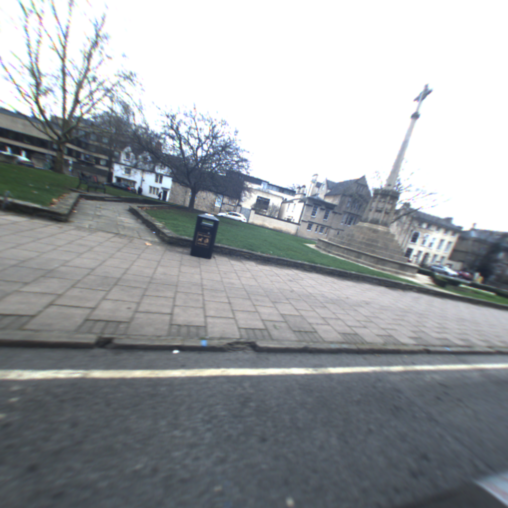
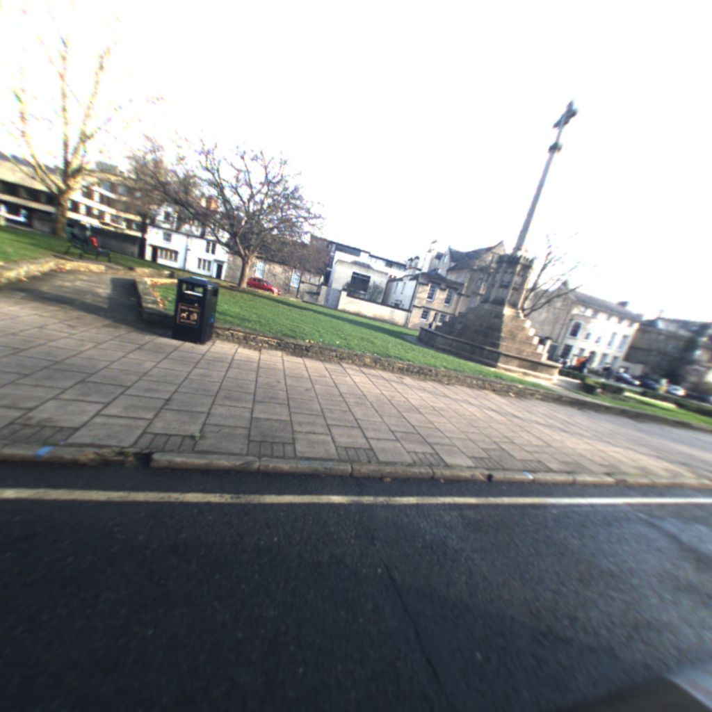
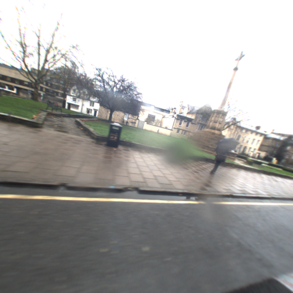
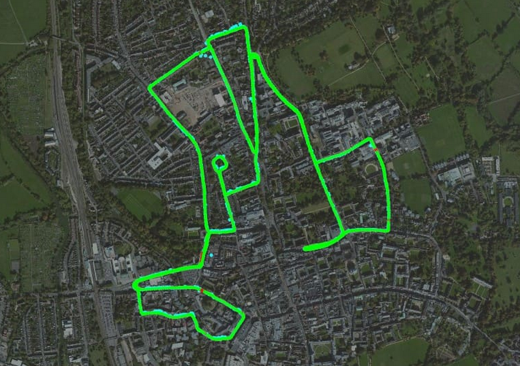
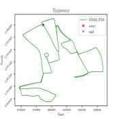
Figure 2: Examples from the Oxford Radar RobotCar outdoor dataset. Top: Images from the same location in the three selected test sequences: a) Reference: cloudy b) Test 01: sunny c) Test 02: rainy (Grasshopper2 left monocular camera). Bottom: the 19 km route of the test sequences, d) satellite view e) GNSS/INS.

To simplify our experiments we selected images from only one of the cameras, the Point Grey Grasshopper2 monocular camera (left), despite the fact that using multiple cameras improve the results. The selected camera points toward the left side of the road and thus encodes the stable urban environment such as the buildings (Figure 2).

From the dataset, we selected sequences for a training set, e.g., supervised fine-tuning, a reference against which the query images from the test sequence are matched and three distinct test sets: 1) the different day but approximately at same time and 2) the different day and different time along with different weather conditions. Table I summarizes different sequences used for training, gallery and testing.

TABLE I: The Radar RobotCar outdoor sequences used in our experiments.

Sequence	Size	Date	Start [GMT]	Condition
Train	37,724	Jan. 10 2019	11:46	Sunny
Reference	36,660	Jan. 10 2019	12:32	Cloudy
Test 01	32,625	Jan. 11 2019	12:26	Sunny
Test 02	28,633	Jan. 16 2019	14:15	Rainy

IV-B COLD

The CoSy Localization Database (COLD) [35] presents annotated data sequences acquired using visual and laser range sensors on a mobile platform. The database represents an effort to provide a large-scale, flexible testing environment for evaluating mainly vision-based topological localization and semantic knowledge extraction methods aiming to work on mobile robots in realistic indoor scenarios. The COLD database consists of several video sequences collected in three different indoor laboratory environments located in three different European cities: the Visual Cognitive Systems Laboratory at the University of Ljubljana, Slovenia; the Autonomous Intelligent Systems Laboratory at the University of Freiburg, Germany; and the Language Technology Laboratory at the German Research Center for Artificial Intelligence in Saarbrücken, Germany.

Data acquisition were performed using three different robotic platforms (an ActivMedia People Bot, an ActiveMedia Pioneer-3 and an iRobot ATRV-Mini) with two Videre Design MDCS2 digital cameras to obtain perspective and omnidirectional views. Each frame is registered with the associated absolute position recovered using laser and odometry data and annotated with a label representing the corresponding place. The data were collected from a path visiting several rooms and under different illumination conditions, including cloudy, night and sunny.

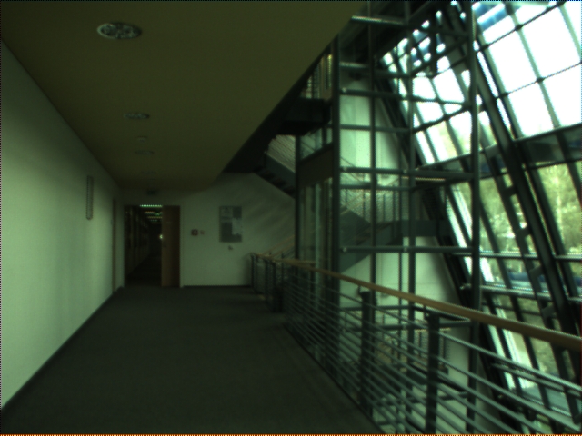
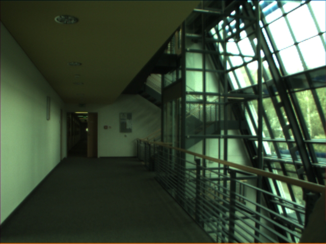
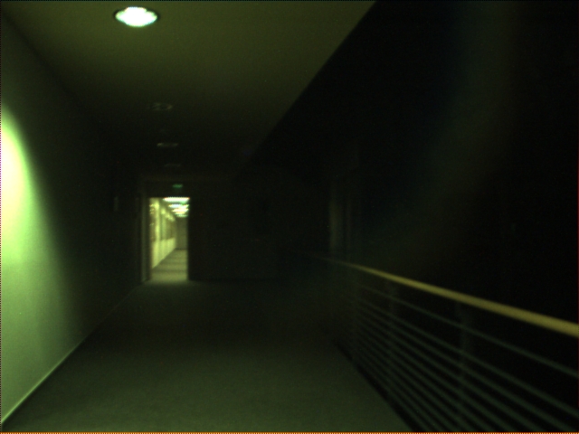
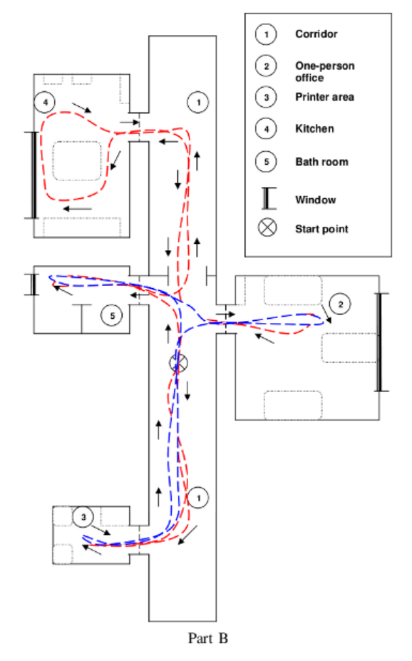
Figure 3: Examples from the COLD indoor database [35]. Images of same location in different sequences: a) Reference: Cloudy-seq1 b) Test 01: Cloudy-seq2, c) Test 02: Night-seq3, d) Map view of the lab: blue dashes: standard path, i.e., short path, red dashes: extended path, arrows indicate the direction of driving the robot and e) Robot path of approximately 50 m.

For our experiments, we selected the extended, e.g., long path on Map B of Saarbrücken laboratory. The training sequence is Sunny-seq3, gallery sequence is Cloudy-seq1, and the three test sequences are 1) Sunny-seq1, 2) Cloudy-seq2 and 3) Night-seq3. See Figure 3 for examples. We used the captured images acquired using the monocular center camera form this setup. Table II summarizes different sequences used for training, reference and testing.

TABLE II: The COLD indoor sequences used in our experiments.

Sequence	Size	Date	Start [GMT]	Condition
Train	1036	July 7 2006	14:59	Sunny
Reference	1371	July 7 2006	17:05	Cloudy
Test 01	1021	July 7 2006	18:59	Cloudy
Test 02	970	July 7 2006	20:34	Night

V Experimental Results

We illustrate the utility of two DCNN architectures with GeM and NetVLAD pooling layers for VPR taks, trained and fine-tuned for the indoor and outdoor VPR datasets with three different loss functions. The experiments aim to address the following research questions: 1) what is the accuracy level of place recognition? 2) what is the impact of fine tuning with different loss functions, given Euclidean space distance or angular space?

Given the reference database and query images, we extract the sparse feature vectors and compute the similarity between each query image and the reference database using $L_{2}$ distance metric. Similar reference feature vectors have the lowest $L_{2}$ distance with the query. Similar to [36], we calculate Fraction of Correct Matches (FCM) as follows:

$$FCM=\frac{Correct\;Matches}{\sum Query\;Images}\times 100,$$ (8)

which corresponds to the proportion of the query images which are correctly matched within a certain accuracy threshold $\tau$.

V-A Oxford Radar RobotCar

Depending on which loss function we utilized to fine-tune the DCNN-based VPR methods for Oxford Radar RobotCar dataset, we report the FCM for two test queries. For this dataset, we report the results within meter accuracy threshold, e.g., $\tau=2\sim 25\;m$.

TABLE III: FCM for Oxford Radar RobotCar dataset, given trained and fine-tuned model with Triplet, Contrastive and ArcFace loss function.

Method	BB	$\tau=25~{}m$	$\tau=10~{}m$	$\tau=5~{}m$	$\tau=2~{}m$
		TRIPLET
Test 01 (diff. day, same time)
GeM [23]	VGG16	90.89	89.36	60.11	42.21
	ResNet50	95.18	93.40	61.61	47.88
NetVLAD [26]	VGG16	56.59	48.89	38.42	17.01
	ResNet50	57.82	51.60	42.13	23.83
Test 02 (diff. day and time)
GeM [23]	VGG16	89.09	86.63	82.92	62.53
	ResNet50	91.74	88.92	84.20	64.86
NetVLAD [26]	VGG16	38.48	31.61	24.55	24.07
	ResNet50	47.69	42.94	37.72	22.23
		CONTRASTIVE
Test 01 (diff. day, same time)
GeM [23]	VGG16	72.69	70.30	64.33	31.92
	ResNet50	71.84	68.41	60.71	32.71
NetVLAD [26]	VGG16	47.30	42.44	33.90	14.03
	ResNet50	50.02	46.67	34.86	14.19
Test 02 (diff. day and time)
GeM [23]	VGG16	60.38	58.94	56.05	42.78
	ResNet50	56.88	52.51	48.39	33.87
NetVLAD [26]	VGG16	30.94	25.53	20.69	11.13
	ResNet50	41.94	38.33	32.09	18.30
		ARCFACE
Test 01 (diff. day, same time)
GeM [23]	VGG16	91.37	89.37	66.16	42.02
	ResNet50	96.51	94.08	68.91	48.09
NetVLAD [26]	VGG16	36.11	25.53	22.40	9.65
	ResNet50	70.54	63.35	52.42	23.83
Test 02 (diff. day and time)
GeM [23]	VGG16	89.64	86.63	82.83	62.42
	ResNet50	92.00	89.00	84.62	65.08
NetVLAD [26]	VGG16	33.58	28.05	23.12	13.36
	ResNet50	49.68	44.46	38.07	22.23

Table III indicate that ArcFace loss function outperforms the triplet and contrastive losses by approximately $1\sim 4\;\%$ when utilized in training time. Furthermore, supervised fine-tuning of the DCNN with GeM pooling layer demonstrates higher robustness in finding the correct matches for queries in the reference dataset, e.g., higher FCM.

V-B COLD

In this section, we present FCM results for the indoor COLD database, given the trained and fine-tuned models with GeM and NetVLAD pooling layers and Tiplet, Contrastive and ArcFace loss functions. For indoor dataset, we report the results within centimeter accuracy threshold, e.g., $\tau=25\sim 100\;cm$.

TABLE IV: FCM for COLD database, given trained and fine-tuned model with Triplet, Contrastive and ArcFace loss function.

Method	BB	$\tau=100~{}cm$	$\tau=75~{}cm$	$\tau=50~{}cm$	$\tau=25~{}cm$
		TRIPLET
Test 01 (cloudy)
GeM [23]	VGG16	94.32	90.11	82.66	46.33
	ResNet50	93.18	94.03	84.62	46.52
NetVLAD [26]	VGG16	90.60	85.80	75.51	43.98
	ResNet50	92.65	89.72	79.53	45.05
Test 02 (night)
GeM [23]	VGG16	84.54	82.47	75.26	43.71
	ResNet50	90.10	85.94	80.21	46.72
NetVLAD [26]	VGG16	75.88	74.33	65.26	42.99
	ResNet50	78.25	77.32	67.73	42.68
		CONTRASTIVE
Test 01 (cloudy)
GeM [23]	VGG16	89.23	86.58	79.33	43.19
	ResNet50	94.52	91.77	85.01	47.40
NetVLAD [26]	VGG16	88.54	83.64	74.24	42.21
	ResNet50	90.40	87.46	76.49	45.05
Test 02 (night)
GeM [23]	VGG16	80.82	78.35	71.86	44.12
	ResNet50	82.06	79.48	73.30	44.54
NetVLAD [26]	VGG16	74.23	72.37	65.05	41.03
	ResNet50	75.05	74.12	66.60	42.89
		ARCFACE
Test 01 (cloudy)
GeM [23]	VGG16	95.10	91.48	83.25	48.19
	ResNet50	96.53	94.32	84.75	46.33
NetVLAD [26]	VGG16	89.52	82.57	72.18	43.78
	ResNet50	91.19	87.56	78.65	45.05
Test 02 (night)
GeM [23]	VGG16	86.60	83.61	76.19	44.64
	ResNet50	93.45	86.49	81.14	47.01
NetVLAD [26]	VGG16	76.08	74.43	66.39	42.06
	ResNet50	72.37	69.59	62.68	37.22

According to Table IV, trained and fine-tuned models with ArcFace loss functions results in more robust performance, $1\sim 2\;\%$, for finding the correct matches in reference database. Moreover, GeM pooling layer outperforms NetVLAD when utilized as a global feature vectors.

We used VGG16 and ResNet50 backbones in our investigations. Although the size of the COLD indoor dataset is relatively smaller than Oxford Radar RobotCar and results of ResNet50 approximately outperforms VGG16, it is computationally more affordable to utilize the VGG16 architecture as the backbone due to smaller size.

VI Conclusion

In this paper, we presented a through investigation of DCNN-based VPR methods, primarily trained and fine-tuned in an end-to-end manner with two pooling layers, e.g., GeM and NetVLAD along with three different loss functions, e.g., triplet, contrastive and ArcFace loss functions.

First, the outperforming validity of supervised fine-tuning the DCNN architechtures, purely trained for classification problems, is comprehensively studied for two real world datasets designed for place recognition in variety of challenging conditions, including seasonal and illumination variations.

Second, the results of correctly matched queries with reference database indicate that supervised fine-tuning the DCNN architectures with ArcFace loss outperforms triplet and contrastive losses for indoor and outdoor datasets within a certain accuracy threshold. Our findings also demonstrate that GeM pooling layer outperforms NetVLAD to extract global feature vectors in both indoor and outdoor datasets.

References

- [1] X. Zhang, L. Wang, and Y. Su, “Visual place recognition: A survey from deep learning perspective,” Pattern Recognition, p. 107760, 2020.
- [2] Z. Xin, X. Cui, J. Zhang, Y. Yang, and Y. Wang, “Visual place recognition with cnns: From global to partial,” in 2017 Seventh International Conference on Image Processing Theory, Tools and Applications (IPTA), 2017, pp. 1–6.
- [3] M. Tzelepi and A. Tefas, “Deep convolutional learning for content based image retrieval,” Neurocomputing, vol. 275, pp. 2467 – 2478, 2018.
- [4] J. Wan, D. Wang, S. C. H. Hoi, P. Wu, J. Zhu, Y. Zhang, and J. Li, “Deep learning for content-based image retrieval: A comprehensive study,” in Proceedings of the 22nd ACM International Conference on Multimedia, ser. MM ’14. New York, NY, USA: Association for Computing Machinery, 2014, p. 157–166.
- [5] J. Gu, Z. Wang, J. Kuen, L. Ma, A. Shahroudy, B. Shuai, T. Liu, X. Wang, G. Wang, J. Cai, and T. Chen, “Recent advances in convolutional neural networks,” Pattern Recognition, vol. 77, pp. 354 – 377, 2018.
- [6] X. Ou, H. Ling, L. Yan, and M. Liu, “Convolutional neural codes for image retrieval,” in Signal and Information Processing Association Annual Summit and Conference (APSIPA), 2014 Asia-Pacific, 2014, pp. 1–10.
- [7] R. R. Saritha, V. Paul, and P. G. Kumar, “Content based image retrieval using deep learning process,” Cluster Comput., vol. 22, no. 2, pp. 4187–4200, Mar 2019.
- [8] B. Cao, A. Araújo, and J. Sim, “Unifying deep local and global features for efficient image search,” ArXiv, vol. abs/2001.05027, 2020.
- [9] M. J. Milford and G. F. Wyeth, “Seqslam: Visual route-based navigation for sunny summer days and stormy winter nights,” in 2012 IEEE International Conference on Robotics and Automation, 2012, pp. 1643–1649.
- [10] M. Cummins and P. Newman, “Appearance-only slam at large scale with fab-map 2.0,” The International Journal of Robotics Research, vol. 30, no. 9, pp. 1100–1123, 2011. [Online]. Available: https://doi.org/10.1177/0278364910385483
- [11] H. Jégou, M. Douze, C. Schmid, and P. Pérez, “Aggregating local descriptors into a compact image representation,” in 2010 IEEE Computer Society Conference on Computer Vision and Pattern Recognition, 2010, pp. 3304–3311.
- [12] Z. Chen, O. Lam, A. Jacobson, and M. Milford, “Convolutional neural network-based place recognition,” ArXiv, vol. abs/1411.1509, 2014.
- [13] P. Sermanet, D. Eigen, X. Zhang, M. Mathieu, R. Fergus, and Y. LeCun, “Overfeat: Integrated recognition, localization and detection using convolutional networks,” 2014.
- [14] N. Sünderhauf, S. Shirazi, F. Dayoub, B. Upcroft, and M. Milford, “On the performance of convnet features for place recognition,” in 2015 IEEE/RSJ International Conference on Intelligent Robots and Systems (IROS), Sep. 2015, pp. 4297–4304.
- [15] Z. Chen, A. Jacobson, N. Sünderhauf, B. Upcroft, L. Liu, C. Shen, I. Reid, and M. Milford, “Deep learning features at scale for visual place recognition,” in 2017 IEEE International Conference on Robotics and Automation (ICRA), 2017, pp. 3223–3230.
- [16] M. Lopez-Antequera, R. Gomez-Ojeda, N. Petkov, and J. Gonzalez-Jimenez, “Appearance-invariant place recognition by discriminatively training a convolutional neural network,” Pattern Recognition Letters, vol. 92, pp. 89 – 95, 2017.
- [17] S. Garg, N. Suenderhauf, and M. Milford, “Don’t look back: Robustifying place categorization for viewpoint- and condition-invariant place recognition,” in 2018 IEEE International Conference on Robotics and Automation (ICRA), 2018, pp. 3645–3652.
- [18] Y. Hou, H. Zhang, and S. Zhou, “Convolutional neural network-based image representation for visual loop closure detection,” in 2015 IEEE International Conference on Information and Automation, 2015, pp. 2238–2245.
- [19] H. Jégou and O. Chum, “Negative Evidences and Co-occurences in Image Retrieval: The Benefit of PCA and Whitening,” in Computer Vision – ECCV 2012. Berlin, Germany: Springer, Oct 2012, pp. 774–787.
- [20] H. Azizpour, A. S. Razavian, J. Sullivan, A. Maki, and S. Carlsson, “From generic to specific deep representations for visual recognition,” in 2015 IEEE Conference on Computer Vision and Pattern Recognition Workshops (CVPRW), 2015, pp. 36–45.
- [21] A. B. Yandex and V. Lempitsky, “Aggregating local deep features for image retrieval,” in 2015 IEEE International Conference on Computer Vision (ICCV), 2015, pp. 1269–1277.
- [22] Y. Kalantidis, C. Mellina, and S. Osindero, “Cross-Dimensional Weighting for Aggregated Deep Convolutional Features,” in Computer Vision – ECCV 2016 Workshops. Cham, Switzerland: Springer, Sep 2016, pp. 685–701.
- [23] F. Radenović, G. Tolias, and O. Chum, “Fine-tuning cnn image retrieval with no human annotation,” IEEE Transactions on Pattern Analysis and Machine Intelligence, vol. 41, no. 7, pp. 1655–1668, 2019.
- [24] G. Tolias, R. Sicre, and H. Jégou, “Particular object retrieval with integral max-pooling of cnn activations,” 2016.
- [25] A. Gordo, J. Almazán, J. Revaud, and D. Larlus, “End-to-End Learning of Deep Visual Representations for Image Retrieval,” Int. J. Comput. Vision, vol. 124, no. 2, pp. 237–254, Sep 2017.
- [26] R. Arandjelovic, P. Gronat, A. Torii, T. Pajdla, and J. Sivic, “NetVLAD: Cnn architecture for weakly supervised place recognition,” TPAMI, 2018.
- [27] H. Noh, A. Araujo, J. Sim, T. Weyand, and B. Han, “Large-scale image retrieval with attentive deep local features,” in 2017 IEEE International Conference on Computer Vision (ICCV), 2017, pp. 3476–3485.
- [28] F. Radenović, G. Tolias, and O. Chum, “CNN image retrieval learns from BoW: Unsupervised fine-tuning with hard examples,” in ECCV, 2016.
- [29] D. G. Lowe, “Distinctive Image Features from Scale-Invariant Keypoints,” Int. J. Comput. Vision, vol. 60, no. 2, pp. 91–110, Nov 2004.
- [30] Q. Wang, Y. Ma, K. Zhao, and Y. Tian, “A Comprehensive Survey of Loss Functions in Machine Learning,” Ann. Data. Sci., pp. 1–26, Apr 2020.
- [31] S. Chopra, R. Hadsell, and Y. LeCun, “Learning a similarity metric discriminatively with application to face verification,” in CVPR, 2005.
- [32] F. Schroff, D. Kalenichenko, and J. Philbin, “Facenet: A unified embedding for face recognition and clustering,” in 2015 IEEE Conference on Computer Vision and Pattern Recognition (CVPR), 2015, pp. 815–823.
- [33] J. Deng, J. Guo, N. Xue, and S. Zafeiriou, “Arcface: Additive angular margin loss for deep face recognition,” in 2019 IEEE/CVF Conference on Computer Vision and Pattern Recognition (CVPR), 2019, pp. 4685–4694.
- [34] D. Barnes, M. Gadd, P. Murcutt, P. Newman, and I. Posner, “The oxford radar robotcar dataset: A radar extension to the oxford robotcar dataset,” in 2020 IEEE International Conference on Robotics and Automation (ICRA), 2020, pp. 6433–6438.
- [35] A. Pronobis and B. Caputo, “Cold: The cosy localization database,” The International Journal of Robotics Research, vol. 28, no. 5, pp. 588–594, 2009. [Online]. Available: https://doi.org/10.1177/0278364909103912
- [36] F. Aliajni and E. Rahtu, “Deep learning off-the-shelf holistic feature descriptors for visual place recognition in challenging conditions,” in 2020 IEEE 22nd International Workshop on Multimedia Signal Processing (MMSP), 2020, pp. 1–6.