Joint Statistics of Cosmological Constant and SUSY Breaking in Flux Vacua with Nilpotent Goldstino

Abstract

We obtain the joint distribution of the gravitino mass and the cosmological constant in KKLT and LVS models with anti-D3 brane uplifting described via the nilpotent goldstino formalism. Moduli stabilisation (of both complex structure and Kähler moduli) is incorporated so that we sample only over points corresponding to vacua. Our key inputs are the distributions of the flux superpotential, the string coupling and the hierarchies of warped throats. In the limit of zero cosmological constant, we find that both in KKLT and LVS the distributions are tilted favourably towards lower scales of supersymmetry breaking.

1 Introduction

Phenomenologically attractive string compactifications can be obtained by turning on background fluxes Michelson:1996pn ; Dasgupta:1999ss ; Gukov:1999ya ; Curio:2000sc ; Giddings:2001yu . In the type IIB setting, the effect of fluxes is to stabilise the complex structure moduli and axio-dilaton Giddings:2001yu . Furthermore, in type IIB there are various scenarios for the stabilisation of the Kähler moduli Kachru:2003aw ; Balasubramanian:2005zx ; vonGersdorff:2005bf ; Berg:2005yu ; Westphal:2006tn ; Cicoli:2008va ; Cicoli:2012fh ; Gallego:2017dvd ; Cicoli:2016chb ; Antoniadis:2018hqy ; AbdusSalam:2020ywo ; Cicoli:2015ylx . This has made type IIB flux compactifications the setting for various detailed phenomenological explorations.

The introduction of fluxes also leads to the possibility of a large multitude of solutions. Apart from construction of detailed models, string phenomenology involves developing an understanding of the broad properties of vacua. The later has motivated the statistical approach to string phenomenology Douglas:2003um ; Cole:2019enn ; Ashok:2003gk ; Denef:2004ze ; Denef:2004dm ; Denef:2004cf (see also Marchesano:2004yn ; Dienes:2006ut ; Gmeiner:2005vz ; Douglas:2006xy ; Acharya:2005ez ; Giryavets:2004zr ; Misra:2004ky ; Conlon:2004ds ; DeWolfe:2005gy ; Hebecker:2006bn ; Martinez-Pedrera:2012teo ; Halverson:2018cio ; Betzler:2019kon ; Bena:2021wyr ; Krippendorf:2021uxu ; Susskind:2004uv ; Douglas:2004qg ; Dine:2004is ; Arkani-Hamed:2005zuc ; Kallosh:2004yh ; Dine:2005yq ; Broeckel:2020fdz ; Broeckel:2021dpz ; Halverson:2019cmy ; Mehta:2020kwu ; Carifio:2017bov ). The distribution of the scale of supersymmetry breaking in the space of string vacua is of course of much interest (see Susskind:2004uv ; Douglas:2004qg ; Dine:2004is ; Arkani-Hamed:2005zuc ; Dienes:2006ut ; Kallosh:2004yh ; Dine:2005yq for early work in this direction). The goal of this paper is to study the joint distribution of the gravitino mass (which sets the scale of supersymmetry breaking in the visible sector in these models) and the cosmological constant in the two most well developed scenarios for Kähler moduli stabilisation in type IIB: KKLT Kachru:2003aw and LVS Balasubramanian:2005zx models. In addition to the scenario for moduli stabilisation, the quantities of interest also depend on the uplift sector of the models. This paper will focus on models where the uplift sector is an anti-brane at the tip of a warped throat (as in the construction of Kachru:2003aw ).

The key ingredients for our analysis will be moduli stabilisation and a systematic incorporation of the effect of the anti-brane via the nilpotent goldstino formalism. Let us describe them in detail.

• Incorporation of moduli stabilisation (both complex structure and Kähler): The values of the cosmological constant and the gravitino mass (and other observables) in a vacuum are determined by the expectation value of the moduli fields. Thus, in order to study the distribution of observables, it is important to incorporate moduli stabilisation and compute the distributions sampling only over points corresponding to the minima of the moduli potential. Early statistical analysis of observables incorporated the stabilisation of complex structure moduli; the importance of Kähler moduli stabilisation was instead emphasised recently in Broeckel:2020fdz . Here, the effect of Kähler moduli stabilisation on the distribution of the gravitino mass was studied. It was found that this has a significant effect on the statistics. Following Broeckel:2020fdz we will sample only over points corresponding to minima of the moduli potential.

• Incorporation of the uplift sector: In both KKLT and LVS, a crucial contribution to the cosmological constant comes from the so-called uplift sector. Before the incorporation of this sector into the effective action, the vacua obtained are necessarily AdS. Furthermore, the cosmological constant and the gravitino mass are correlated in these vacua. Before considering the uplift sector, KKLT vacua are supersymmetric. Thus (setting $M_{P}=1$)

  $$\hat{V}_{\rm KKLT}=-3\hat{m}^{2}_{3/2}\,,$$ (1.1)

  where the hat indicates a quantity computed in the effective field theory before adding the uplift sector. Similarly for LVS vacua (before uplifting)

  $$\hat{V}_{\rm LVS}\simeq-\hat{m}^{3}_{3/2}\,,$$ (1.2)

  The relations (1.1) and (1.2) are broken solely due to introduction of the uplift sector. Thus it is crucial to incorporate it while computing the joint distribution of the cosmological constant and the gravitino mass.

  Of course, there are various effects that can lead to an uplift. We shall focus on an anti-D3 brane at the bottom of a warped throat. The reasons for this are the following:

  • The nilpotent superfield formalism: The nilpotent superfield formalism allows for explicit computation of the effect of an anti-D3 brane in a warped throat. The effects of the anti-brane are captured by the introduction of a nilpotent chiral superfield $X$ such that $X^{2}=0$ (see for instance Rocek:1978nb ; Ivanov:1978mx ; Lindstrom:1979kq ; Casalbuoni:1988xh ; Komargodski:2009rz and references therein). $X$ has a single propagating component, the Volkov-Akulov goldstino Volkov:1973ix , and supersymmetry is broken by its F-term. The effective couplings of such a field $X$ were studied in Farakos:2013ih ; Antoniadis:2014oya ; Bergshoeff:2015tra ; Dudas:2015eha ; Antoniadis:2015ala ; Hasegawa:2015bza ; Kallosh:2015tea ; DallAgata:2015pdd ; Schillo:2015ssx ; Kallosh:2015pho and the KKLT uplifting term was reproduced within the supergravity framework in Bergshoeff:2015jxa ; Kallosh:2014wsa ; Kallosh:2015nia . Finally, in Kallosh:2015nia explicit string constructions were presented in which an anti-D3-brane at the bottom of a warped throat has only the goldstino as its light degree of freedom, justifying the use of the nilpotent field $X$ to describe the anti-brane. Soft masses in KKLT and LVS were computed using this framework in Aparicio:2015psl .

  • Distribution of throat hierarchies: For uplift with anti-D3 branes in warped throats, the magnitude of the uplift term is set by the hierarchy associated with the warped throat. Thus an understanding of the distribution of throat hierarchies is needed to understand the distribution of physical observables in this setting. The distribution of throat hierarchies has been studied in detail in Hebecker:2006bn . We will make heavy use of these results.

Our main finding is that the distribution of the gravitino mass at zero cosmological constant is tilted towards lower values. This is not the same as the result of Douglas:2004qg (see also Susskind:2004uv ) which carried out generic estimates on supersymmetry breaking F- and D-terms and concluded that there is a preference for high scale breaking. Note that this result is different also from the one of Broeckel:2020fdz which found a logarithmic preference for high scales of supersymmetry breaking after stabilising the Kähler moduli but before uplifting. The difference arises due to the presence of the relations (1.1) and (1.2) and the form of the distribution for throat hierarchies. Our results should not be taken as giving the generic picture for string vacua. In fact, in some class of models such as Saltman:2004jh high scale breaking is essentially in-built. At the same time, we find it very interesting that the best understood models have distributions favouring lower masses of the gravitino.

This paper is organised as follows. In Sec. 2 we review some material that will be needed for our analysis. In Sec. 3 we compute the joint distribution for the gravitino mass and cosmological constant in LVS and KKLT models with anti-D3 brane uplifting. We discuss our results and conclude in Sec. 4. We will closely follow the notation and conventions of Aparicio:2015psl .

2 Review

In this section we review material that will be needed for our analysis. We will touch upon 3 topics: ($i$) warped throats in type IIB flux compactifications, ($ii$) the statistical distribution of parameters that appear in the effective field theory of the Kähler moduli, and ($iii$) the nilpotent goldstino formalism.

2.1 Warped throats in IIB flux compactifications

In this subsection we review some aspects of warped throats in flux compactifications that will be useful for this paper. Type IIB flux compactifications have 3-form fluxes (NSNS and RR) threading the 3-cycles of an orientifolded Calabi-Yau (CY). The back-reaction of fluxes has the effect of generating warping (as in Randall:1999ee ). The 10D metric takes the form Giddings:2001yu ; Dasgupta:1999ss

$$\differential s_{10}^{2}=e^{2A(y)}\eta_{\mu\nu}\differential{x^{\mu}}\differential{x^{\nu}}+e^{-2A(y)}g_{mn}\differential{y^{m}}\differential{y^{n}},\$$ (2.1)

where $e^{2A(y)}\equiv h^{-1/2}(y)$ is the warp factor and $g_{mn}$the CY metric. The warp factor satisfies a Poisson-like equation which is sourced by 3-form fluxes and localised objects carrying D3-charge. For non-vanishing fluxes, the warp factor varies over the compact directions. The warp factor acts like a redshift factor for the objects localised in the compact directions. In regions where $e^{-2A}$ is large, it can be used to generate hierarchies in physical scales. Regions of large warping arise when fluxes thread the 3-cycle associated with a conifold modulus and its dual cycle. The geometry in this region is close to that of the Klebanov-Strassler (KS) throat Klebanov:2000hb . Our primary interest will be in the regime in which the warp factor is almost constant over the whole compact space, except for a single throat where the geometry is highly warped.

As pointed out in Giddings:2005ff , a constant shift of $e^{4A}$ maps solutions of the Poisson equation to solutions, and this freedom is to be identified with (a power of) the volume modulus. Furthermore, a pure scaling of the CY metric $\differential s_{CY}^{2}$ to a unit-volume fiducial metric $\differential s_{CY_{0}}^{2}$, given by $\differential s_{CY}^{2}\to\lambda\differential s_{CY}^{2}$, implies a rescaling of the warp factor $e^{2A}\to\lambda e^{2A}$, and hence has no effect on the physical geometry. Given this, a useful parametrisation of the 10D geometry is

$$\differential{s^{2}_{10}}=\mathcal{V}^{1/3}\left(e^{-4A_{0}}+\mathcal{V}^{2/3}\right)^{-1/2}\differential{s^{2}_{4}+}\left(e^{-4A_{0}}+\mathcal{V}^{2/3}\right)^{1/2}\differential{s_{CY_{0}}^{2}}\>,$$ (2.2)

which is equivalent to:

$$\differential{s^{2}_{10}}=\left(1+\frac{e^{-4A_{0}}}{\mathcal{V}^{2/3}}\right)^{-1/2}\differential{s^{2}_{4}+}\left(1+\frac{e^{-4A_{0}}}{\mathcal{V}^{2/3}}\right)^{1/2}\differential{s_{CY}^{2}}\>.$$ (2.3)

The factor $\left(1+\frac{e^{-4A_{0}}}{\mathcal{V}^{2/3}}\right)^{-1/4}\equiv\Omega$ is the redshift factor. In a highly warped region, $e^{-4A_{0}}\gg\mathcal{V}^{2/3}$ and $\Omega\sim e^{A_{0}}\mathcal{V}^{1/6}\ll 1$. It is important to keep the following in mind:

1. In highly warped regions generated where the local geometry of the underlying CY is close to that of a conifold, the spacetime metric is close to the KS geometry:

   $$\differential{s^{2}_{10}}=e^{2A(r)}\differential{s^{2}_{4}}+e^{-2A(r)}\left(\differential{r^{2}}+r^{2}\differential{s^{2}_{T^{1,1}}}\right)\>,$$ (2.4)

   The presence of the fluxes resolves the conifold singularity, and one has a minimal area 3-sphere at the bottom of the throat. The warp factor takes its minimal value on this 3-sphere Giddings:2001yu

   $$e^{4A_{\rm min}}\sim e^{-\frac{8\pi K}{3g_{s}M}}\equiv y\>,$$ (2.5)

   where $g_{s}$ is the string coupling and $K$ and $M$ are the integral fluxes that thread the 3-sphere and its dual cycle.

2. The hierarchy in (2.5) is related to the value at which the (shrinking) conifold modulus $|z|$ is stabilised Giddings:2001yu . They are related as follows:

   $$y=|z|^{4/3}.$$

   Note that this relation implies that the statistical distribution of the stabilised value of $|z|$ determines the distribution of the hierarchy $y$.

3. The warped volume $\mathcal{V}_{W}$ which relates the 10D and 4D Planck masses is given by

   $$\mathcal{V}_{W}=\int\differential[6]{y}\sqrt{g_{\small{CY}}}\,e^{-4A}=\mathcal{V}\int\differential[6]{y}\sqrt{g_{CY_{0}}}\left(1+\frac{e^{-4A_{0}}}{\mathcal{V}^{2/3}}\right)\sim\mathcal{V}\,,$$ (2.6)

   where the last approximation is valid if the volume of the throat region is small compared to the (large) CY volume. Note that the warped volume remains finite even when regions of large warping are present. This is related to the finiteness of the Kähler potential in the complex structure moduli space.

4. The 10D action of an anti-D3 brane can be used to compute its contribution to the 4D scalar potential. This crucially depends on the anti-D3 position $\vec{r}_{{\rm D3}}$ in the internal dimensions, i.e. whether it is in a warped or unwarped region:

   $$V_{\rm\overline{D3}}=2T_{3}\int\differential[4]{x}\sqrt{-g_{4}}\sim\frac{2M_{s}^{4}\,\mathcal{V}^{2/3}}{e^{-4A(r_{{\rm D3}})}+\mathcal{V}^{2/3}} \sim \left\{\begin{array}[]{lcl}\frac{e^{4A(r_{{\rm D3}})}}{\mathcal{V}^{4/3}}&\rm{for}&e^{-4A(r_{{\rm D3}})}\gg\mathcal{V}^{2/3}\\ \frac{1}{\mathcal{V}^{2}}&\rm{for}&\mathcal{V}^{2/3}\gg e^{-4A(r_{{\rm D3}})}\\ \end{array}\right.$$ (2.9)

   where $T_{3}$ is the tension of the brane.

5. Note that in the absence of warping one has a string scale contribution to the potential which typically will lead to a run away. Thus warped throats are necessary to obtain stable vacua in the presence of anti-D3 branes. On the other hand, a large volume is necessary to keep the $\alpha^{\prime}$ expansion valid. In the presence of both large warping and large volume it is important to understand the interplay between these two large quantities and the regime of validity of the effective field theory. This has been analysed in detail in Giddings:2005ff ; Burgess:2006mn ; Cicoli:2012fh . One finds the requirement

   $$e^{-A_{0}}\ll\mathcal{V}^{2/3}\ll e^{-4A_{0}}\,.$$ (2.10)

   We emphasise that in the very large radius limit, i.e. $\mathcal{V}^{2/3}\gg e^{-4A_{0}(y)}$ at all points in the compact directions, the metric becomes the standard unwarped CY metric $\differential{s_{10}^{2}}=\differential{s_{4}^{2}}+\mathcal{V}^{1/3}\differential{s_{CY_{0}}^{2}}=\differential{s_{4}^{2}}+\differential{s_{CY}^{2}}$. In this limit there are no throats, and hence this region of moduli space is not appropriate if one wants to uplift KKLT and LVS AdS vacua.

2.2 Distributions of $W_{0}$, string coupling and hierarchy of throats

As emphasised in the introduction, the properties of a string vacuum are determined by the values at which moduli are stabilised. Our focus will be on KKLT and LVS models. Here fluxes stabilise the complex structure moduli. The Kähler moduli continue to remain flat after the introduction of fluxes. The stabilisation of the Kähler moduli can be studied in a low energy effective theory where the complex structure moduli are integrated out. Although the number of fluxes can be large, their effect on the low energy effective field theory of the Kähler moduli is encoded in terms of a small number of parameters. For the observables that interest us, these are: the expectation value of the Gukov-Vafa-Witten superpotential $W_{0}$, the dilaton $g_{s}$ and the hierarchy associated with the bottom of the warped throat $y$. The statistical distributions of these quantities will serve as input for determining the distributions of the observables. The distributions of $W_{0}$, $g_{s}$ and $y$ have been well studied. Below, we describe them.

• The expectation value of the Gukov-Vafa-Witten superpotential $W_{0}$ is uniformly distributed as a complex variable Denef:2004ze and physical quantities will be functions of $|W_{0}|$. Given the flat distribution of $W_{0}$, the distribution for $|W_{0}|$ is proportional to $|W_{0}|$. The distribution of $W_{0}$ and its physical implications were analysed in detail in Cicoli:2013swa .

• The distribution of the dilaton is known to be uniform Ashok:2003gk ; Denef:2004ze . In terms of the axio-dilaton $S=s-iC_{0}$ with $s=1/g_{s}$

  $$\differential{\mathcal{N}}={\differential{S}\over s^{2}}\,,$$ (2.11)

  where $\differential{S}=\differential{s}\differential{C_{0}}$ is the integration measure over the axio-dilaton. This has been confirmed by various numerical and analytic studies (see e.g. Broeckel:2020fdz ; Blanco-Pillado:2020wjn ).

• Finally, we turn to the hierarchy $y$. As discussed in Sec. 2.1, the hierarchy is determined by the vacuum expectation value of the shrinking conifold modulus $|z|$. The distribution for $|z|$ (as determined by stabilisation from fluxes) was studied in Denef:2004ze . The fraction of vacua in which the conifold modulus takes value below $|z|$ was found to be

  $$f(|z|)=-{C\over\ln{|z|}}\,,$$ (2.12)

  where $C$ is a positive constant. The corresponding density is

  $$\mathcal{N}(|z|)\differential{|z|}={C\differential{|z|}\over|z|(\ln{|z|)^{2}}}\,.$$ (2.13)

  It is important to keep in mind that the singularity in the density for small $|z|$ is benign. Arbitrarily small $|z|$ corresponds to arbitrary large fluxes, which would be in conflict with the D3-tadpole cancellation condition. The statistical description is expected to break down before the singularity. Related is the fact that the fraction of states as given in (2.12) vanishes in the limit of $|z|\to 0$. Although, note that there is a significant enhancement of states in comparison with the expectation from the canonical metric of $\mathbb{C}$.

  This distribution was used to study the distribution of throat hierarchies and the expectations for the number of throats in Hebecker:2006bn . It was found that throats are ubiquitous.

Before closing this subsection, we would like to record an important point in the analysis of Hebecker:2006bn which will be useful for our study. It was argued in Hebecker:2006bn that if one is dealing with a CY with a large number of flux quanta, the joint distribution of 2 (or a small number of) quantities which are not related through a functional relation is proportional to the product of the 2 individual distributions. For example, if one considers 2 conifold moduli $|z_{1}|$ and $|z_{2}|$, then these are determined by independent fluxes (hence are functionally independent), and so the joint distribution is

$$\mathcal{N}(|z_{1}|,|z_{2}|)\differential{|z_{1}|}\differential{|z_{2}|}\propto\mathcal{N}(|z_{1}|)\mathcal{N}(|z_{2}|)\differential{|z_{1}|}\differential{|z_{2}|}\,.$$ (2.14)

Similar considerations also apply when one is considering the joint distribution of a conifold modulus and a quantity that is a function of a large number of fluxes. The product structure in the joint distribution essentially follows from the fact that when there is a large number of fluxes, fixing one quantity should not affect the distribution of another quantity significantly unless there is a functional relation between them. See Hebecker:2006bn for a more detailed discussion.

2.3 Effective field theory of the nilpotent goldstino

Spontaneous supersymmetry breaking in (effective) supergravity theories leads to the super-Higgs effect – the gravitino eats the goldstino to become massive. If this phenomenon takes place at energies which are low compared with the Planck mass, the goldstino couplings can be described by making use of a (constrained) independent superfield. Supersymmetry is then non-linearly realised as in the Volkov-Akulov formalism. There are several approaches to describe the low energy dynamics of the goldstino in terms of spurion or constrained superfields (see for instance Komargodski:2009rz and references therein). Our focus will be on the approach where the goldstino is described in terms of a chiral superfield $X$ that is constrained to be nilpotent, i.e. $X^{2}=0$. This has the ingredients necessary to describe supersymmetry breaking induced by the presence of an anti-D3 brane at the tip of a warped throat in flux compactifications Bergshoeff:2015jxa ; Kallosh:2014wsa ; Kallosh:2015nia .

The effective field theory involving a nilpotent chiral superfield $X$ can be described in terms of a Kähler potential $K$, a superpotential $W$ and a gauge kinetic function $f$ whose general forms are:

$$K=K_{0}+K_{1}X+\bar{K}_{1}\bar{X}\ +K_{2}X\bar{X},\qquad W=\rho X+\tilde{W},\qquad f=f_{0}+f_{1}X,$$ (2.15)

where $K_{0}$, $K_{1}$, $K_{2}$, $\rho$, $\tilde{W}$, $f_{0}$, $f_{1}$ are functions of other low energy fields. Higher powers of $X$ are absent in $K$ and $W$ since $X^{2}=0$. The nilpotency condition implies a constraint on the components of $X$. Expanding $X$ in superspace

$$X=X_{0}(y)+\sqrt{2}\psi(y)\theta+F(y)\theta\bar{\theta}\>,$$ (2.16)

(where as usual, $y^{\mu}=x^{\mu}+i\theta\sigma^{\mu}\bar{\theta}$), $X^{2}=0$ implies

$$X_{0}=\frac{\psi\psi}{2F}\>.$$ (2.17)

Thus unless the fermion $\psi$ condenses in the vacuum, the vacuum expectation value of $X_{0}$ (the scalar component of $X$) vanishes.

For an anti-D3 brane at the bottom of a warped throat of a type IIB flux compactification, the description in terms of $X$ is very convenient. It allows to treat its effects in terms of supergravity: its contribution to the scalar potential, the gravitino mass and the couplings to moduli and matter fields are easily obtained. It was shown in Kallosh:2015nia that nilpotent superfield(s) capture all degrees of freedom of an anti-D3 brane when it is placed on top of an orientifold plane. The presence of the fluxes and the orientifold projection leave the massless goldstino as a low energy propagating degree of freedom, in keeping with the use of a nilpotent superfield $X$ to describe the system. The simplest example is that of an O3-plane and an anti-D3 brane at the bottom of a warped throat. In this case, there is no modulus associated with the position of the anti-D3 brane (in contrast to the case of D3-branes in the bulk). This corresponds to the fact that the scalar component of $X$ is not a propagating field. Furthermore, there is no contribution from $X_{0}$ to the scalar potential and it can be consistently set to zero while looking for vacuum solutions.

Next, let us turn to the form of the Kähler potential and superpotential in (2.15). In the case of a single Kähler modulus $T$ ($T=\mathcal{V}^{2/3}+i\psi\equiv\tau+i\psi$ is a complex field obtained by pairing the volume modulus and its axionic partner), the functions $\tilde{W}$ and $\rho$ have no dependence on $T$ at the perturbative level, as a result of holomorphy and the Peccei-Quinn shift symmetry $T\mapsto T+ic$. The zeroth order term in the Kähler potential of (2.15), $K_{0}=-2\ln\mathcal{V}$ is invariant (up to a Kähler transformation) under the full modular transformation $T\rightarrow(aT-ib)/(icT+d)$ (which is a generalisation of the shift symmetry). If $X$ transforms suitably, i.e. as a modular form of weight $\kappa$, the quadratic coefficient takes the form $K_{2}=\beta\tau^{-\kappa}$ (where $\beta$ is a constant). Moreover, if the term linear in $X$ is absent, the only contribution of $X$ to the F-term potential is a positive definite term:

$$V_{\rm up}=e^{K}K^{-1}_{X\bar{X}}\left\|\frac{\partial W}{\partial X}\right\|^{2}=\frac{|\rho|^{2}}{\tau^{3-\kappa}}\>.$$ (2.18)

This precisely coincides with form of the contribution of an anti-D3 brane at the tip of a warped throat with hierarchy ${|\rho|^{2}\big{/}\beta}$ as computed from direct dimensional reduction (see equation (2.9)), if the modular weight is $\kappa=1$. Since the anti-D3 brane is localised at a particular point in the compactification manifold, direct couplings to gauge fields located at distant D3 or D7-branes are difficult. This implies the absence of terms linear in $X$ in the gauge kinetic functions. In summary, at leading order in the $\alpha^{\prime}$ expansion the effective field theory is specified by:

$$K=-2\ln\mathcal{V}+\beta\frac{X\bar{X}}{\tau},\qquad W=\tilde{W}+\rho X,\qquad f=f_{0}\,,$$ (2.19)

where $c$, $\rho$, $\tilde{W}$, $f_{0}$ are constants and $|\rho|^{2}/\beta$ is identified with the hierarchy $y$ as defined in (2.5), i.e. $y=|\rho|^{2}/\beta$. Furthermore, the superpotential only receives non-perturbative corrections. Nilpotency of $X$ implies that the Kähler potential in (2.19) can be written as:

$$K=-3\ln\left(\tau-\frac{\beta}{3}X\bar{X}\right)\>.$$ (2.20)

Note that in the regime where the effective field theory is valid, i.e. when the anti-D3 brane is at the tip of a warped throat, the $X$ superfield couples to $T$ in the Kähler potential in the same way a superfield $\phi$ describing the D3-brane matter fields, i.e. Grana:2003ek ; Grimm:2004uq

$$K_{\text{D3}}=-3\ln\left(\tau-\frac{\alpha}{3}\phi\bar{\phi}\right)\sim-2\ln\mathcal{V}+\alpha\frac{\phi\bar{\phi}}{\tau}+\cdots\>,$$ (2.21)

where the dots indicate terms which are higher order in the $1/\tau$ expansion. It is then natural to conjecture Aparicio:2015psl that the only effect of $X$ in the Kähler potential is to shift the Kähler coordinate $T$ in the same way as the field $\phi$ does. This was called the log hypothesis, as it leads one to write the $X\bar{X}$ term inside the log as in (2.20).

When both D3-branes and anti-D3-brane are present, generically the Kähler potential can be written as

$$K=-2\ln\mathcal{V}+\alpha\frac{\phi\bar{\phi}}{\tau^{\mu}}+\beta\frac{X\bar{X}}{\tau^{\kappa}}+\gamma\frac{X\bar{X}\,\phi\bar{\phi}}{\tau^{\zeta}}+\cdots\,,$$ (2.22)

with modular weights $\mu=\kappa=1$ as discussed above. Moreover, if $\phi$ and $X$ have modular weights $\mu$ and $\kappa$ respectively, the modular weight for the $X\bar{X}\,\phi\bar{\phi}$ term should be $\zeta=\mu+\kappa$. In this case, $\zeta=1+1=2$. This agrees with the log hypothesis, i.e. a Kähler potential of the form

$$K_{\rm no-scale}=-3\ln\left(\tau-\frac{\alpha}{3}\phi\bar{\phi}-\frac{\beta}{3}X\bar{X}\right)\,.$$ (2.23)

In fact, expanding this in powers of $1/\tau$, one obtains (2.22) with the condition that $\gamma=\frac{\alpha\beta}{3}$. The Kähler potential in (2.23) is of the standard no-scale form Cremmer:1983bf ; Burgess:2020qsc .

We conclude this subsection with comments relevant for the computation of soft masses. In the KKLT scenario, the low energy effective theory is usually written in terms of the fields with masses of order or below the gravitino mass. These include massless chiral fields (arising as excitations of open strings) and the Kähler moduli. Supersymmetry is broken at the minimum of the scalar potential. Both the F-term of $X$ and the F-term of $T$ are different from zero (with $F^{T}\ll F^{X}$). Thus, the goldstino is a combination of the fermion in $X$ and the fermion in $T$. In LVS, even in the absence of the anti-brane, the overall volume modulus $T_{b}$ breaks supersymmetry ($F^{T_{b}}\neq 0$). Inclusion of the nilpotent superfield in the effective action allows one to consider the breaking of supersymmetry induced by fluxes and supersymmetry breaking by the anti-brane on equal footing. Again, the goldstino is a combination of the fermion components of $X$ and of the moduli. Although the dominant component is usually the one from the $T_{b}$-field, for sequestered models the $X$ component is relevant and its contribution to the soft terms must be accounted for.

3 Joint gravitino mass and cosmological constant distribution

In this section we will evaluate the joint distribution of the gravitino mass and the cosmological constant for KKLT and LVS models with anti-brane uplifting. As described earlier, we will make use of the distributions of the axio-dilaton, $W_{0}$ and $y$ (the hierarchy) to evaluate these. We start by writing the expression for the number of vacua in an infinitesimal volume in these coordinates. Making use of the results discussed in Sec. 2.2, we have

$$\differential{\mathcal{N}}={\eta|W_{0}|\over{y(\ln y)^{2}s^{2}}}\differential{|W_{0}|}\differential{S}\differential{y},$$ (3.1)

where we have made use of the fact that the hierarchy is related to the size of the shrinking conifold modulus by $y=|z|^{4/3}$ ($\differential{S}$ is the measure for integration over the axio-dilaton: $\differential{S}=\differential{s}\differential{C_{0}}$). We have also taken the number of fluxes to be large, so justifying the factorised form of the density. In both KKLT and LVS the cosmological constant and the gravitino mass can be expressed in terms of $|W_{0}|$, $y$ and $s$. We will use these expressions to carry out a change of variables in (3.1). This will provide us with the required densities.

3.1 KKLT

With the complex structure moduli and the dilaton stabilised by fluxes, we will take the low energy fields to be the Kähler moduli, chiral matter and the nilpotent superfield. For simplicity, we will consider one Kähler modulus $T$ and matter fields living on D3-branes which we will collectively denote as $\phi$. Then

$$K=-2\ln{\mathcal{V}}+\tilde{K}_{i}\ \phi\bar{\phi}+\tilde{Z}_{i}\ X\bar{X}+\tilde{H}_{i}\ \phi\bar{\phi}\ X\bar{X}+...\>,$$ (3.2)

where $\tilde{K}_{i}$ and $\tilde{Z}_{i}$ are the Kähler metrics for the matter field on D3-branes and the nilpotent goldstino. $\tilde{H}_{i}$ is the quartic interaction between the matter field and the nilpotent goldstino. As per the discussion in Sec. 2.3, these are

$$\tilde{K}_{i}=\frac{\alpha}{\tau}\>,\qquad\tilde{Z}_{i}=\frac{\beta}{\tau}\>,\qquad\tilde{H}_{i}=\frac{\gamma}{\tau^{2}}\>,$$ (3.3)

where the scaling of $\tilde{K}_{i}$ with $\tau$ is due to the modular weight of the matter field on D3-branes Conlon:2006tj ; Aparicio:2008wh . The superpotential is

$$W\ =\ W_{0}+\rho X+A\ e^{-aT}\>,$$ (3.4)

where we have included a non-perturbative contribution in $T$ which is needed to stabilise the Kähler modulus. The KKLT construction requires $|W_{0}|\ll 1$ (see e.g. Demirtas:2021nlu ; Demirtas:2019sip ; Cole:2019enn ; Broeckel:2021uty ; Cicoli:2022vny and references therein for recent works on explicit construction of vacua with low values of $|W_{0}|$). We will study the statistical distributions for fixed values of $a$ and $A$.

Recall that the supergravity scalar potential is determined in terms of the Kähler potential and the superpotential as

$$V=e^{K}\left(K^{I\bar{J}}D_{I}WD_{\bar{J}}\bar{W}-3|W|^{2}\right)\qquad\mbox{with}\qquad D_{I}W=\partial_{I}W+K_{I}W\>,$$ (3.5)

where the indices $I$ and $J$ run over the chiral superfields $T,\phi,X$. $K^{I\bar{J}}$ is the inverse of the matrix $K_{I\bar{J}}\equiv\partial_{I}\partial_{\bar{J}}K$ and $K_{I}\equiv\partial_{I}K$. It is often convenient to write (3.5) as

$$V=F^{I}F_{I}-3m_{3/2}^{2}\,,$$ (3.6)

where $F_{I}\equiv e^{K/2}D_{I}W$ and $F^{I}\equiv e^{K/2}K^{I\bar{J}}D_{\bar{J}}\bar{W}$ are the F-terms. The gravitino mass is instead given by $m_{3/2}\equiv e^{K/2}|W|$.

By making use of (3.2) and (3.4) in (3.5), one finds

$$V=\left(V_{\text{KKLT}}+V_{\text{up}}\right)+\frac{2}{3}\left((V_{\text{KKLT}}+V_{\text{up}})+\frac{1}{2}V_{\text{up}}\left(1-\frac{3\gamma}{\alpha\beta}\right)\right)\ |\hat{\phi}|^{2}\>,$$ (3.7)

where the scalar component of the nilpotent field is set to zero (assuming no condensation of fermions). $V_{\text{KKLT}}$ is the KKLT potential in the absence of the uplifting term:

$$V_{\text{KKLT}}\ =\ \frac{2\ e^{-2a\tau}aA^{2}}{s\ \mathcal{V}^{4/3}}+\frac{2\ e^{-2a\tau}a^{2}A^{2}}{3s\ \mathcal{V}^{2/3}}\ -\frac{2\ e^{-a\tau}aA\ W_{0}}{s\ \mathcal{V}^{4/3}}\,.$$ (3.8)

To reduce clutter in the equations we have followed the standard practice of writing both $W_{0}$ and $A$ real and positive. For general values of $W_{0}$ and $A$ the expression for the potential can be obtained from the above by taking $W_{0}\to|W_{0}|$ and $A\to|A|$. We have also neglected the overall contribution from the Kähler potential for the complex structure moduli which is an order one multiplicative factor. The imaginary part of $T$ (the axion $\psi$) has its minimum at $\psi=\pi/a$. This is responsible for the negative sign in the third term in (3.8). The uplift term $V_{\text{up}}$ arises from $F^{X}F_{X}$ and is given by

$$V_{\text{up}}=\frac{\rho^{2}}{2\beta s\tau^{2}}\equiv\frac{y}{2s\tau^{2}}\qquad\text{with}\qquad y=\frac{\rho^{2}}{\beta}\,.$$ (3.9)

The third contribution in (3.7) is proportional to $|\hat{\phi}|^{2}$ with $\hat{\phi}$ denoting the canonically normalised matter scalar field $\phi$. This contribution corresponds to its soft mass. For non-tachyonic scalars, the vacuum expectation value of $\hat{\phi}$ would vanish, and so we will proceed by setting $\hat{\phi}=0$. Soft masses will be discussed in Sec. 4.

Minimising the scalar potential, one finds that the following holds at the minimum

$$W_{0}=e^{-a\tau}A\left(1+\frac{2}{3}a\tau+\frac{y\,e^{2a\tau}}{2a^{2}A^{2}\tau}\right)\,,$$ (3.10)

where we have dropped subleading terms in the $(a\tau)^{-1}$ expansion multiplying the term proportional to $y$. In what follows, we shall drop such subleading terms, but shall include their effect in the numerical results that we will present later. Using (3.10) in the expression for the scalar potential (3.7), its value at the minimum is found to be

$$\Lambda=-\frac{2e^{-2a\tau}a^{2}A^{2}}{3s\ \tau}+\frac{y}{2s\tau^{2}}\equiv\left(V_{\text{KKLT}}^{(0)}+V_{\text{up}}\right).$$ (3.11)

Note that the hierarchy $y$ can be tuned to make the cosmological constant zero or extremely small and positive. For a Minkowski vacuum one needs

$$y=\frac{4}{3}\,\tau\,e^{-2a\tau}a^{2}A^{2}\,.$$ (3.12)

The gravitino mass becomes

$$m_{3/2}=e^{K/2}|W|={1\over\sqrt{2s}}{1\over\tau^{3/2}}\left(W_{0}-A\,e^{-a\tau}\right).$$ (3.13)

Next, we turn to evaluating the joint distribution for the gravitino and cosmological constant. For this, we will perform the change of variables $(W_{0},y,S)\to(m_{3/2},\Lambda,S)$ in (3.1). We need to compute the Jacobian of this transformation. The expressions for the cosmological constant and the gravitino mass ((3.11) and (3.13)) have explicit dependence on $(W_{0},y,s)$ and also implicit dependence via $\tau$. To compute the partial derivatives of the cosmological constant and the gravitino mass with respect to $W_{0}$ and $y$ we need to compute the partial derivatives of $\tau$ with respect to these variables. Making use of (3.10), we find

$${\partial\tau\over\partial y}=-{e^{a\tau}\over 2Aa^{2}\tau f(\tau)}\,,$$ (3.14)

with

$$f(\tau)=Ae^{-a\tau}\left(-{2\over 3}a^{2}\tau\left(1+{1\over 2a\tau}\right)+{{y\,e^{2a\tau}}\over{2aA^{2}\tau}}\left(1-{1\over a\tau}\right)\right)\,.$$ (3.15)

Now let us turn to the entries of the Jacobian. These are

$${\partial m_{3/2}\over\partial W_{0}}={1\over\sqrt{2s}}{1\over\tau^{3/2}}+\left({1\over\sqrt{2s}}{1\over\tau^{3/2}}aAe^{-a\tau}-{3\over 2\tau}m_{3/2}\right){\partial\tau\over\partial W_{0}}\,,$$ (3.16)

$${\partial m_{3/2}\over\partial y}=\left({1\over\sqrt{2s}}{1\over\tau^{3/2}}aAe^{-a\tau}-{3\over 2\tau}m_{3/2}\right){\partial\tau\over\partial y}\,.$$ (3.17)

We also have

$${\partial\Lambda\over\partial W_{0}}={\partial\Lambda\over\partial\tau}{\partial\tau\over\partial W_{0}}\,,\qquad\qquad{\partial\Lambda\over\partial y}={\partial\Lambda\over\partial\tau}{\partial\tau\over\partial y}+{1\over 2s\tau^{2}}\,,$$ (3.18)

with

$${\partial\Lambda\over\partial\tau}={4e^{-2a\tau}a^{3}A^{2}\over 3s\tau}\left(1+{1\over 2a\tau}\right)-{y\over s\tau^{3}}\,,$$ (3.19)

3.1.1 Analytical estimate

The expressions in (3.16), (3.17) and (3.18) are rather cumbersome. While we will use them for our numerical analysis in Sec. 3.1.2, we continue our analytic investigation in a regime that leads to considerable simplifications. For this, we define the quantity $x$ as

$$x\equiv{{y\,e^{2a\tau}}\over{2a^{2}A^{2}\tau}}\,,$$ (3.20)

which allows to write (3.11) as

$$\Lambda=-\frac{2e^{-2a\tau}a^{2}A^{2}}{3s\,\tau}\left(1-\frac{3}{2}\,x\right)=-3m_{3/2}^{2}\left(1-\frac{3}{2}\,x\right)\left(1+\frac{3}{2a\tau}\,x\right)^{-2}\,.$$ (3.21)

We shall now focus on the regime in which $y$ is varied such that $0<x\lesssim\mathcal{O}(1)\ll(a\tau)$. Comparing with (3.21) we see that this allows for uplift to zero and positive values of the cosmological constant. Hence, the regime covers the region of most interest since $x\gg 1$ corresponds to an unstable situation where the uplifting contribution would yield a runaway. Also note that in this regime, the contribution of the term involving $y$ in right hand side of (3.10) becomes subdominant. We can therefore take the approximation

$$W_{0}=e^{-a\tau}A\left(1+\frac{2}{3}a\tau+x\right)\simeq{2\over 3}A(a\tau)e^{-a\tau}\,,$$ (3.22)

and so, to leading order in the $(a\tau)^{-1}$ expansion, we have

$$\tau\simeq-{1\over a}\ln\left({3\over 2A}W_{0}\right),$$ (3.23)

and the gravitino mass looks like

$$m_{3/2}\simeq{W_{0}\over{\sqrt{2s}\tau^{3/2}}}={2\over 3}{{(a\tau)A}\over{\sqrt{2s}\tau^{3/2}}}e^{-a\tau}\,.$$ (3.24)

This allows us to write

$$\tau\simeq-{1\over a}\ln\left(3\sqrt{{s\over 2}}{{m_{3/2}\over{a^{3/2}A}}}\right)\,.$$ (3.25)

In the regime we are considering, we can write (3.11) as

$$y\simeq 2s\tau^{2}\left(\Lambda+3m^{2}_{3/2}\right)\,.$$ (3.26)

Combining this with (3.25) we can express $y$ in terms of $\Lambda$, $m_{3/2}$ and $s$. Similarly, making use of (3.25) in (3.24) gives $W_{0}$ in terms of the same quantities.

The Jacobian entries undergo significant simplifications in this regime where the function $f(\tau)$ defined in (3.15) becomes $f(\tau)\simeq-{2\over 3}a^{2}Ae^{-a\tau}\tau$. We then have

$${\partial\tau\over\partial W_{0}}\simeq-{3\over 2Aa^{2}\tau}e^{a\tau}\,,\qquad\qquad{\partial\tau\over\partial y}\simeq{3\over 4A^{2}a^{4}\tau^{2}}e^{2a\tau}\,.$$ (3.27)

Let us turn to the partial derivatives of $m_{3/2}$. First note that by making use of (3.10) and (3.13) one can write

$$m_{3/2}={Ae^{-a\tau}\over\tau^{3/2}(2s)^{1/2}}\left({2\over 3}a\tau+{y\,e^{2a\tau}\over 2a^{2}A^{2}\tau}\right)\equiv{Ae^{-a\tau}\over\tau^{3/2}(2s)^{1/2}}\left({2\over 3}a\tau+x\right)\,.$$ (3.28)

Recall now that

$${\partial m_{3/2}\over\partial W_{0}}={1\over\sqrt{2s}}{1\over\tau^{3/2}}+\left({1\over\sqrt{2s}}{1\over\tau^{3/2}}aAe^{-a\tau}-{3\over 2\tau}m_{3/2}\right){\partial\tau\over\partial W_{0}}\,.$$ (3.29)

Making use of $(\ref{m3oth})$, we see that

$$\left({1\over\sqrt{2s}}{1\over\tau^{3/2}}aAe^{-a\tau}-{3\over 2\tau}m_{3/2}\right)=-{3\over 2}{Ae^{-a\tau}\over\tau^{5/2}(2s)^{1/2}}\,x\,.$$ (3.30)

Using (3.27) and (3.30) in (3.29), and the fact that in the above equation $0<x\lesssim\mathcal{O}(1)$, we see that the term proportional to ${\partial\tau\over\partial W_{0}}$ is always subleading in (3.29). Therefore we have

$${\partial m_{3/2}\over\partial W_{0}}\simeq{1\over\sqrt{2s}}{1\over\tau^{3/2}}\,.$$ (3.31)

Similarly, using the above formulae, one finds

$${\partial m_{3/2}\over\partial y}\simeq-{9\sqrt{a}\over 8A}{1\over\sqrt{2s}}{1\over(a\tau)^{9/2}}\,e^{a\tau}x\,.$$ (3.32)

Now, let us come to the derivatives of $\Lambda$. Note that the ratio of the two terms in (3.11) is $-{3\over 4}x$. Given this (and the fact that $0<x\lesssim\mathcal{O}(1)$), comparing the various terms in $(\ref{ltau})$ gives

$${\partial\Lambda\over\partial\tau}\simeq{4e^{-2a\tau}a^{3}A^{2}\over 3s\tau}\,.$$ (3.33)

Combining this with (3.18) and (3.27) one finds

$${\partial\Lambda\over\partial W_{0}}\simeq-{2Aa^{3}\over s}{e^{-a\tau}\over(a\tau)^{2}}\qquad\text{and}\qquad{\partial\Lambda\over\partial y}\simeq{1\over 2s\tau^{2}}\,.$$ (3.34)

Combining (3.31), (3.32) and (3.34), the Jacobian is

$$J\simeq{1\over(2s)^{3/2}}{1\over\tau^{7/2}}\,.$$ (3.35)

Finally, we have

$$\differential{\mathcal{N}}={\eta\,W_{0}\over{y(\ln y)^{2}s^{2}}}\differential{W_{0}}\differential{y}\differential{s}={\eta\,W_{0}\over{y(\ln y)^{2}s^{2}}}|J|^{-1}\differential{m_{3/2}}\differential{\Lambda}\differential{S}\,.$$ (3.36)

Equations (3.24), (3.25) and (3.26) can be used to express this density in terms of the desired quantities. We find

$$\differential{\mathcal{N}}={2\tau^{3}m_{3/2}\over{\left(3m^{2}_{3/2}+\Lambda\right)\left[\ln\left(2s\tau^{2}(3m^{2}_{3/2}+\Lambda)\right)\right]^{2}s}}\,\differential{m_{3/2}}\differential{\Lambda}\differential{S}\,.$$ (3.37)

To get the expression for the joint distribution of $m_{3/2}$ and $\Lambda$, we need to perform the integration over the axio-dilaton moduli space. However, the important features can be extracted by analysing the above density at fixed values of the axio-dilaton $(s,C_{0})$. Note that in the $|\Lambda|\ll m^{2}_{3/2}$ limit (which is physically most interesting) the density scales as

$$\rho_{\rm KKLT}(\Lambda\simeq 0)\simeq{\ln m_{3/2}\over m_{3/2}}\,,$$ (3.38)

implying that it is tilted favourably towards lower values of $m_{3/2}$.

This result can be understood as follows. Let us think of uplifting various AdS vacua obtained before the introduction of the uplift term. These vacua are supersymmetric and $\Lambda=-3m_{3/2}^{2}$. The introduction of the uplift term has a very small effect on the value of $m_{3/2}$. Thus, when we consider vacua with cosmological constant close to zero, a vacuum with a low value of $m_{3/2}$ also has a low value of the hierarchy $y$ (as the associated supersymmetric AdS vacuum before the introduction of the uplift has a $\Lambda$ of small magnitude). The distribution of throats is such that it is tilted in favour of lower values of $y$, and this makes the distribution of $m_{3/2}$ favourable towards lower values of $m_{3/2}$.

3.1.2 Numerical results

Let us now present the numerical results which we have obtained for the joint distribution of the cosmological constant and the gravitino mass without making any approximation. Fig. 1 shows the density of states as a function of $m_{3/2}$ for different fixed values of $\Lambda$ corresponding to AdS, Minkowski and dS vacua. In the physically interesting region with $|\Lambda|\ll m^{2}_{3/2}$, the 3 curves approach each other, reproducing the analytical estimate (3.38) where $\rho_{\rm KKLT}$ becomes independent of $\Lambda$ and is inversely proportional to $m_{3/2}$ (up to a logarithmic dependence). Note that the green curve with positive $\Lambda$ features a raising behaviour of $\rho_{\rm KKLT}$ for $m_{3/2}^{2}\lesssim\Lambda$. However this regime can be ignored for the following two reasons: ($i$) it is valid only for a small window of values of $m_{3/2}$ close to $m_{3/2}^{2}\lesssim\Lambda$ since, as can be seen from (3.21), $m_{3/2}^{2}\ll\Lambda$ would require $x\gg 1$ that yields a runaway; ($ii$) the region characterised by $m_{3/2}^{2}\lesssim\Lambda$ is phenomenologically irrelevant since it would correspond to an essentially massless gravitino with $m_{3/2}$ below the Hubble parameter.

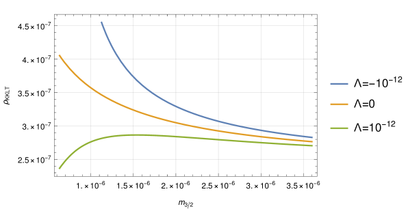
Figure 1: Density of KKLT flux vacua at fixed values of the cosmological constant $\Lambda$ as a function of the gravitino mass $m_{3/2}$ in Planck units.

For completeness, in Fig. 2 we have also plotted the density of vacua as a function of $m_{3/2}$ and $\Lambda$. Note that the two blank regions corresponds respectively to the runaway limit (for positive $\Lambda$) and to the violation of the supergravity lower limit $\Lambda\geq-3m_{3/2}^{2}$ (for negative $\Lambda$).

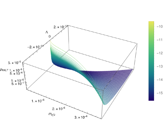
Figure 2: Density of KKLT flux vacua as a function of the gravitino mass $m_{3/2}$ and the cosmological constant $\Lambda$ in Planck units.

3.2 LVS

We now turn to the LVS models. Using the same notation as in the previous subsection, the Kähler potential can be written as

$$K=-2\ln\left(\mathcal{V}+\xi\,s^{3/2}\right)+\tilde{K}_{i}\ \phi\bar{\phi}+\tilde{Z}_{i}\ X\bar{X}+\tilde{H}_{i}\ \phi\bar{\phi}\ X\bar{X}+...\>.$$ (3.39)

We will focus on the simplest LVS example, with two Kähler moduli $T_{s}$ and $T_{b}$ with real parts $\tau_{b}$ and $\tau_{s}$, with the CY volume having a Swiss cheese structure: $\mathcal{V}=\tau_{b}^{3/2}-\tau_{s}^{3/2}$. The coefficients $\tilde{K}_{i}$, $\tilde{Z}_{i}$ and $\tilde{H}_{i}$ are matter metric and quartic interaction coefficients. The superpotential is

$$W\ =\ W_{0}+\rho X+A\ e^{-a_{s}T_{s}}\,$$ (3.40)

where $W_{0}\sim\mathcal{O}(1-10)$ in LVS. The supergravity scalar potential (after setting the matter field expectation values to zero) takes the form:

$$V=V_{\text{LVS}}+V_{\text{up}}\,,$$ (3.41)

where $V_{\text{LVS}}$ is the LVS potential in the absence of the uplift sector

$$V_{\text{LVS}}=\frac{4}{3}\frac{e^{-2a_{s}\tau_{s}}\sqrt{\tau_{s}}\ a_{s}^{2}A^{2}}{s\ \mathcal{V}}-\frac{2e^{-a_{s}\tau_{s}}\tau_{s}\ a_{s}A\ W_{0}}{s\ \mathcal{V}^{2}}+\frac{3\sqrt{s}\ \xi\ W_{0}^{2}}{8\ \mathcal{V}^{3}}\,.$$ (3.42)

In LVS the minimum is non-supersymmetric before the introduction of the uplifting term. Minimising the LVS potential $V_{\text{LVS}}$, one obtains the conditions that the Kähler moduli have to satisfy in the minimum:

$$e^{-a_{s}\tau_{s}}=\frac{3\ \tau_{s}^{1/2}\ W_{0}}{4a_{s}A\ \mathcal{V}}\,,$$ (3.43)

and

$$\tau_{s}^{3/2}=\frac{s^{3/2}\xi}{2}\,.$$ (3.44)

The value of the potential at this minimum is

$$V_{\text{LVS}}^{(0)}=-\frac{3\sqrt{s}\ \xi\ W_{0}^{2}}{16a_{s}\tau_{s}\ \mathcal{V}^{3}}\,.$$ (3.45)

Next, we consider the potential (3.41) that includes the $X$-contribution responsible for uplifting the AdS minimum. The minimum condition (3.43) is not modified, while (3.44) is changed to

$$\tau_{s}^{3/2}={s^{3/2}\xi\over 2}\left(1+{16\over 27}{{\mathcal{V}^{5/3}y}\over{W_{0}^{2}{s^{3/2}\xi}}}\right)\,.$$ (3.46)

For later use, we define

$$x_{\rm LVS}\equiv{16\over 27}{y\,(a_{s}\tau_{s}){\mathcal{V}^{5/3}}\over{W_{0}^{2}{s^{3/2}\xi}}}\,.$$ (3.47)

The value of the potential at the minimum now becomes

$$\Lambda=V_{\text{LVS}}^{(0)}+{5\over 9}\,V_{\rm up}=-{3\sqrt{s}\xi W_{0}^{2}\over 16a_{s}\tau_{s}\mathcal{V}^{3}}+{5\over 9}{y\over 2s\mathcal{V}^{4/3}}=-{3\sqrt{s}\xi W_{0}^{2}\over 16a_{s}\tau_{s}\mathcal{V}^{3}}\left(1-\frac{5}{2}\,x_{\rm LVS}\right)\,,$$ (3.48)

which gives a Minkowski minimum for

$$y={27\over 40}{{W_{0}^{2}{s^{3/2}\xi}}\over{{\mathcal{V}^{5/3}a_{s}\tau_{s}}}}\qquad\Leftrightarrow\qquad x_{\rm LVS}=\frac{2}{5}\,.$$ (3.49)

Thus we realise that (3.48) can allow for uplift to zero and positive values of the cosmological constant provided $y$ is varied so that $x_{\rm LVS}$ lies in the $0<x_{\rm LVS}\lesssim\mathcal{O}(1)\ll(a_{s}\tau_{s})$ regime, with $x_{\rm LVS}\gg 1$ corresponding to the runaway limit. Hence from now on we shall focus just on the interesting region where the potential is stable and the gravitino mass is given by

$$m_{3/2}={W_{0}\over{\sqrt{2s}\,\mathcal{V}}}\,.$$ (3.50)

Let us now perform a variable change in (3.1) to obtain the joint distribution of the gravitino mass and the cosmological constant: $(W_{0},y,s,C_{0})\to(W_{0},\Lambda,m_{3/2},C_{0})$. $\Lambda$ and $m_{3/2}$, given in (3.48) and (3.50), have explicit dependence on $s$ and $y$ and also implicitly depend on the dilaton and the hierarchy via $\tau_{s}$ and $\cal{V}$. Note that, at leading order in the ${(a_{s}\tau_{s})^{-1}}$ expansion, we have ${\partial\mathcal{V}\over\partial\tau_{s}}=a_{s}\mathcal{V}$ and

$${\partial\tau_{s}\over\partial s}={\left({\xi\over 2}\right)^{2/3}\over{1-{10\over 9}x_{\rm LVS}}}\equiv{\left({\xi\over 2}\right)^{2/3}\over\Psi}\,,\qquad{\partial\tau_{s}\over\partial y}=\frac{32}{81}{{\mathcal{V}^{5/3}\tau_{s}}\over{W_{0}^{2}{s^{3/2}\xi}}}{1\over\Psi}=\frac{2}{3}{{x_{\rm LVS}}\over y\,a_{s}\,\Psi}\,.$$ (3.51)

Now we turn to the entries of the Jacobian (again, to leading order in the $(a_{s}\tau_{s})^{-1}$ expansion). They read

$${\partial m_{3/2}\over\partial s}=-a_{s}m_{3/2}{\partial\tau_{s}\over\partial s}\,,\qquad{\partial m_{3/2}\over\partial y}=-a_{s}m_{3/2}{\partial\tau_{s}\over\partial y}\,,$$ (3.52)

$${\partial\Lambda\over\partial s} = -3V_{\rm LVS}^{(0)}a_{s}\Psi{\partial\tau_{s}\over\partial s}=-3V_{\rm LVS}^{(0)}a_{s}\left({\xi\over 2}\right)^{2/3}\,,\qquad{\partial\Lambda\over\partial y}={1\over 2s\mathcal{V}^{4/3}}\,,$$ (3.53)

where we have used (3.51). These give a Jacobian of the form

$$J=-{5\over 18}{{m_{3/2}a_{s}\over\Psi}}\left({\xi\over 2}\right)^{2/3}{1\over{s\mathcal{V}^{4/3}}}=-{5\over 2^{1/3}\,9}\left({\xi\over 2}\right)^{2/3}{{a_{s}m_{3/2}^{7/3}\over\Psi s^{1/3}W_{0}^{4/3}}}\,.$$ (3.54)

From (3.48) we can write

$$y={18\over 5}s\mathcal{V}^{4/3}\left(\Lambda+{3\sqrt{s}\xi W_{0}^{2}\over 16a_{s}\tau_{s}\mathcal{V}^{3}}\right)={2^{1/3}\,9\over 5}{s^{1/3}W_{0}^{4/3}\over m_{3/2}^{4/3}}\left(\Lambda+{3\sqrt{2}\xi m_{3/2}^{3}s^{2}\over 8a_{s}\tau_{s}W_{0}}\right)\,.$$ (3.55)

In summary, we find

$$\differential{\mathcal{N}}={\eta\,W_{0}\over{y(\ln y)^{2}s^{2}}}|J|^{-1}\differential{W_{0}}\differential{m_{3/2}}\differential{\Lambda}\differential{C_{0}},$$ (3.56)

with $J$ and $y$ given in (3.54) and (3.55) and $\tau_{s}=s\left({\xi\over 2}\right)^{2/3}\simeq-{1\over a_{s}}\ln m_{3/2}$. To get the final form of the distribution, one should integrate over $C_{0}$ and $W_{0}$. Even if this is not tractable, the interesting features of the joint distribution can be obtained by considering fixed values of $C_{0}$ and $W_{0}$ (which is an $\mathcal{O}(1-10)$ quantity in LVS). In the physically interesting regime where $|\Lambda|\ll m_{3/2}^{3}$, we can also make the following approximations

$$|J|^{-1}\simeq{(\ln m_{3/2})^{1/3}\over m_{3/2}^{7/3}}\,,\qquad y^{-1}\simeq{1\over(\ln m_{3/2})^{4/3}m_{3/2}^{5/3}}\,,$$ (3.57)

which give

$$\rho_{\rm LVS}(\Lambda\simeq 0)\simeq{1\over(\ln m_{3/2})^{3}m_{3/2}^{4}}\,.$$ (3.58)

Interestingly, we find that the distribution of flux vacua with cosmological constant close to zero is highly tilted towards lower values of $m_{3/2}$. We have confirmed this analytical estimate with an exact numerical evaluation of the density of LVS flux vacua as a function of $m_{3/2}$ and $\Lambda$. Two plots showing these results are presented in Fig. 3 and Fig. 4. As stressed already in the KKLT case, the blank region in Fig. 4 for $\Lambda>0$ would lead to a runaway, while the blank region for $\Lambda<0$ would correspond to a violation of the supergravity lower limit $\Lambda\geq-3m_{3/2}^{2}$.

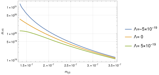
Figure 3: Density of LVS flux vacua at fixed values of the cosmological constant $\Lambda$ as a function of the gravitino mass $m_{3/2}$ in Planck units.

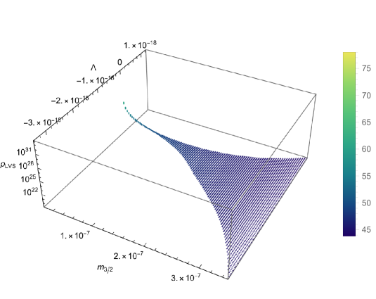
Figure 4: Density of LVS flux vacua as a function of the gravitino mass $m_{3/2}$ and the cosmological constant $\Lambda$ in Planck units.

4 Discussion and conclusions

In this paper we have studied the joint distribution of the gravitino mass and cosmological constant in KKLT and LVS models with the uplift sector arising from an anti-brane at the tip of a warped throat. We have found that, at values of the cosmological constant close to zero, the gravitino mass distribution is tilted favourably towards lower scales. This result is different from that based on generic expectations for the size of F- and D-terms Douglas:2004qg ; Susskind:2004uv , including also moduli stabilisation Broeckel:2020fdz . The form of the distribution of the throat hierarchies and the nature of the AdS vacua before the introduction of the uplift sector leads to this difference. This work gives strong motivation for similar studies in related setups so that a better understanding of the joint statistics of the scale of supersymmetry breaking and the cosmological constant in string vacua can be obtained.

Our results have several interesting implications which we now briefly discuss:

• Distribution of soft terms: Supersymmetry breaking in a hidden sector leads to the generation of soft terms in the visible sector. The strength of supersymmetry breaking in the visible sector is characterised by the size of the scalar masses $m_{0}^{2}$, gaugino masses $M_{1/2}$ and trilinear couplings $A_{ijk}$. In both KKLT and LVS, these depend on how the Standard Model is realised on either D3- or D7-branes. Soft terms for both realisations were analysed in Aparicio:2015psl (see also Aparicio:2014wxa ; Aparicio:2015sda ; Kallosh:2015nia ; Choi:2005ge ; Choi:2005uz ; Falkowski:2005ck ; Lebedev:2006qq ). In the case of D7-branes, all soft terms tend to be of order the gravitino mass. On the other hand, in the case of D3-branes, the models can exhibit sequestering at tree level with non-zero soft masses generated by $\alpha^{\prime}$ and quantum corrections. One can find interesting patterns in the structure of soft masses, allowing for the realisation of MSSM-like spectra or (mini) split supersymmetry. All the soft parameters are of the form $m_{3/2}^{1+p}$ with $p\geq 0$ or $m_{3/2}\big{/}(\ln(m_{3/2}))^{q}$ with $q>0$. This implies that the tilt in the distribution favouring lower values of $m_{3/2}$ also corresponds to the same for the scale of supersymmetry breaking in the visible sector.

• Comparison with data: Statistical distributions of vacua have been used to confront classes of string vacua with data (see e.g. Baer:2019xww ; Baer:2020dri ; Baer:2021vrk ; Baer:2021tta ; Baer:2021zbj ; Baer:2022wxe ; Baer:2022naw ; Baer:2022qqr ) by examining the implications of the distributions of UV parameters for low energy observables. These studies have focused on power-law and logarithmic distributions with a preference for high scale supersymmetry. It will be interesting to carry out similar analysis with our results given that the tilt in favour of low scale supersymmetry is likely to help to make contact with observations or even to generate some tension with data. Of course, this line of study assumes that the distributions computed by studying the distribution of vacua should be translated to distributions for predictions for experiments.

• Multiple throats: The simplest generalisation of our setup is to consider multiple throats (this was studied in the context of supersymmetry breaking in Susskind:2004uv ). We examine it to understand the effect of multiple supersymmetry breaking sectors.

  Let us consider $n$ throats, each with a single anti-brane. Taking $n$ to be small, so that the distribution in the throat sector factorises, we have

  $$\differential{\mathcal{N}_{\rm th}}\propto\prod_{i=1}^{n}{1\over{y_{i}}(\ln y_{i})^{2}}\prod_{i=1}^{n}\differential{y_{i}}\,.$$ (4.1)

  The uplift term is given by

  $$V_{\rm up}={1\over 2s\tau^{2}}\sum_{i=1}^{n}y_{i}\,.$$ (4.2)

  It is useful to make a series of variable changes: $y_{i}=w_{i}^{2}$, then to spherical coordinates in $w_{i}$ (with $r^{2}=\sum_{i=1}^{n}(w_{i})^{2}$) and angular variables ($\theta_{j}$, $j=1,...,(n-1)$) and finally $\tilde{r}=r^{2}$. With this, the distribution (4.3) takes the form

  $$\differential{\mathcal{N}_{\rm th}}\propto{1\over{2\tilde{r}g(\theta_{i})\prod_{i=1}^{n}(\ln w_{i})^{2}}}\differential{\Omega_{n-1}}\differential{\tilde{r}},$$ (4.3)

  where $g(\theta_{i})$ is a function of the angular variable. In these coordinates, the uplift term is given by

  $$V_{\rm up}={\tilde{r}\over 2s\tau^{2}}\,,$$ (4.4)

  it is independent of the angular coordinates and has exactly the same form as the single variable case. To obtain the joint distribution of the gravitino mass and the cosmological constant, consider the full distribution function

  $$\differential{\mathcal{N}}={\eta^{\prime}\,W_{0}\over s^{2}}\differential{S}\differential{W_{0}}\differential{\mathcal{N}_{\rm th}}\,,$$ (4.5)

  and make the variable change $(W_{0},\tilde{r},s,C_{0},\theta_{i})\to(W_{0},\Lambda,m_{3/2},C_{0},\theta_{i})$ for LVS and $(W_{0},\tilde{r},S,\theta_{i})\to(m_{3/2},\Lambda,S,\theta_{i})$ for KKLT. Since the uplift term has the same functional form as in the single variable case, also the functional form of the Jacobian is the same as in the single variable case. As a result, the $\tilde{r}$ dependence of the density is similar to the $y$ dependence in the single variable case. Thus in the $\Lambda\to 0$ limit, the functional dependence on $m_{3/2}$ is the same as in the single throat case (up to logarithmic terms). We conclude that the distribution function of throats is such that adding multiple sectors (but small in number) preserves the tilt in the distribution function in favour of lower values of $m_{3/2}$.

• Sensitivity to uplift: The tilt in the distribution for $m_{3/2}$ towards lower values is tied to the distribution for throat hierarchies. In particular, the $y^{-1}$ factor in the distribution for hierarchies plays a crucial role. Thus our result should not be taken as providing the general picture for the distribution of $m_{3/2}$ and the cosmological constant. In order to gain a general understanding, the distribution has to be studied for various uplift mechanisms (see e.g. Burgess:2003ic ; Westphal:2006tn ; Cicoli:2012fh ; Gallego:2017dvd ; Antoniadis:2018hqy ; Cicoli:2015ylx ). To gain a general understanding of the joint distribution of the supersymmetry breaking and the cosmological constant scales in the whole flux landscape, one should then be able to determine the relative abundance of vacua characterised by different uplifting mechanisms. Our work represents just the first step forward in this direction. We leave this important direction for future work.

• Quantum corrections: The distributions that we have derived make use of the Wilsonian effective field theory obtained at the high compactification scale after integrating out stringy and Kaluza-Klein states. Physical quantities will be however affected by low energy quantum loops. These corrections can be large for the cosmological constant, i.e. ${\mathcal{O}}(m_{3/2}^{4})$, but the conditions used to obtain the small $\Lambda$ limit of the distributions, i.e. $\Lambda\ll m_{3/2}^{2}$ in KKLT and $\Lambda\ll m_{3/2}^{3}$ in LVS, are stable against such corrections. Hence the form of the distribution functions obtained, is expected to be stable against the incorporation of quantum effects.

References

- (1) J. Michelson, Compactifications of type IIB strings to four-dimensions with nontrivial classical potential, Nucl. Phys. B 495 (1997) 127 [hep-th/9610151].
- (2) K. Dasgupta, G. Rajesh and S. Sethi, M theory, orientifolds and G - flux, JHEP 08 (1999) 023 [hep-th/9908088].
- (3) S. Gukov, C. Vafa and E. Witten, CFT’s from Calabi-Yau four folds, Nucl. Phys. B 584 (2000) 69 [hep-th/9906070].
- (4) G. Curio, A. Klemm, D. Lust and S. Theisen, On the vacuum structure of type II string compactifications on Calabi-Yau spaces with H fluxes, Nucl. Phys. B 609 (2001) 3 [hep-th/0012213].
- (5) S.B. Giddings, S. Kachru and J. Polchinski, Hierarchies from fluxes in string compactifications, Phys. Rev. D 66 (2002) 106006 [hep-th/0105097].
- (6) S. Kachru, R. Kallosh, A.D. Linde and S.P. Trivedi, De Sitter vacua in string theory, Phys. Rev. D 68 (2003) 046005 [hep-th/0301240].
- (7) V. Balasubramanian, P. Berglund, J.P. Conlon and F. Quevedo, Systematics of moduli stabilisation in Calabi-Yau flux compactifications, JHEP 03 (2005) 007 [hep-th/0502058].
- (8) G. von Gersdorff and A. Hebecker, Kahler corrections for the volume modulus of flux compactifications, Phys. Lett. B 624 (2005) 270 [hep-th/0507131].
- (9) M. Berg, M. Haack and B. Kors, On volume stabilization by quantum corrections, Phys. Rev. Lett. 96 (2006) 021601 [hep-th/0508171].
- (10) A. Westphal, de Sitter string vacua from Kahler uplifting, JHEP 03 (2007) 102 [hep-th/0611332].
- (11) M. Cicoli, J.P. Conlon and F. Quevedo, General Analysis of LARGE Volume Scenarios with String Loop Moduli Stabilisation, JHEP 10 (2008) 105 [0805.1029].
- (12) M. Cicoli, A. Maharana, F. Quevedo and C.P. Burgess, De Sitter String Vacua from Dilaton-dependent Non-perturbative Effects, JHEP 06 (2012) 011 [1203.1750].
- (13) D. Gallego, M.C.D. Marsh, B. Vercnocke and T. Wrase, A New Class of de Sitter Vacua in Type IIB Large Volume Compactifications, JHEP 10 (2017) 193 [1707.01095].
- (14) M. Cicoli, D. Ciupke, S. de Alwis and F. Muia, Inflation: moduli stabilisation and observable tensors from higher derivatives, JHEP 09 (2016) 026 [1607.01395].
- (15) I. Antoniadis, Y. Chen and G.K. Leontaris, Perturbative moduli stabilisation in type IIB/F-theory framework, Eur. Phys. J. C 78 (2018) 766 [1803.08941].
- (16) S. AbdusSalam, S. Abel, M. Cicoli, F. Quevedo and P. Shukla, A systematic approach to Kähler moduli stabilisation, JHEP 08 (2020) 047 [2005.11329].
- (17) M. Cicoli, F. Quevedo and R. Valandro, De Sitter from T-branes, JHEP 03 (2016) 141 [1512.04558].
- (18) M.R. Douglas, The Statistics of string / M theory vacua, JHEP 05 (2003) 046 [hep-th/0303194].
- (19) A. Cole, A. Schachner and G. Shiu, Searching the Landscape of Flux Vacua with Genetic Algorithms, JHEP 11 (2019) 045 [1907.10072].
- (20) S. Ashok and M.R. Douglas, Counting flux vacua, JHEP 01 (2004) 060 [hep-th/0307049].
- (21) F. Denef and M.R. Douglas, Distributions of flux vacua, JHEP 05 (2004) 072 [hep-th/0404116].
- (22) F. Denef, M.R. Douglas and B. Florea, Building a better racetrack, JHEP 06 (2004) 034 [hep-th/0404257].
- (23) F. Denef and M.R. Douglas, Distributions of nonsupersymmetric flux vacua, JHEP 03 (2005) 061 [hep-th/0411183].
- (24) F. Marchesano, G. Shiu and L.-T. Wang, Model building and phenomenology of flux-induced supersymmetry breaking on D3-branes, Nucl. Phys. B 712 (2005) 20 [hep-th/0411080].
- (25) K.R. Dienes, Statistics on the heterotic landscape: Gauge groups and cosmological constants of four-dimensional heterotic strings, Phys. Rev. D 73 (2006) 106010 [hep-th/0602286].
- (26) F. Gmeiner, R. Blumenhagen, G. Honecker, D. Lust and T. Weigand, One in a billion: MSSM-like D-brane statistics, JHEP 01 (2006) 004 [hep-th/0510170].
- (27) M.R. Douglas and W. Taylor, The Landscape of intersecting brane models, JHEP 01 (2007) 031 [hep-th/0606109].
- (28) B.S. Acharya, F. Denef and R. Valandro, Statistics of M theory vacua, JHEP 06 (2005) 056 [hep-th/0502060].
- (29) A. Giryavets, S. Kachru and P.K. Tripathy, On the taxonomy of flux vacua, JHEP 08 (2004) 002 [hep-th/0404243].
- (30) A. Misra and A. Nanda, Flux vacua statistics for two-parameter Calabi-Yau’s, Fortsch. Phys. 53 (2005) 246 [hep-th/0407252].
- (31) J.P. Conlon and F. Quevedo, On the explicit construction and statistics of Calabi-Yau flux vacua, JHEP 10 (2004) 039 [hep-th/0409215].
- (32) O. DeWolfe, Enhanced symmetries in multiparameter flux vacua, JHEP 10 (2005) 066 [hep-th/0506245].
- (33) A. Hebecker and J. March-Russell, The Ubiquitous throat, Nucl. Phys. B 781 (2007) 99 [hep-th/0607120].
- (34) D. Martinez-Pedrera, D. Mehta, M. Rummel and A. Westphal, Finding all flux vacua in an explicit example, JHEP 06 (2013) 110 [1212.4530].
- (35) J. Halverson and F. Ruehle, Computational Complexity of Vacua and Near-Vacua in Field and String Theory, Phys. Rev. D 99 (2019) 046015 [1809.08279].
- (36) P. Betzler and E. Plauschinn, Type IIB flux vacua and tadpole cancellation, Fortsch. Phys. 67 (2019) 1900065 [1905.08823].
- (37) I. Bena, J. Blabäck, M. Graña and S. Lüst, Algorithmically Solving the Tadpole Problem, Adv. Appl. Clifford Algebras 32 (2022) 7 [2103.03250].
- (38) S. Krippendorf, R. Kroepsch and M. Syvaeri, Revealing systematics in phenomenologically viable flux vacua with reinforcement learning, 2107.04039.
- (39) L. Susskind, Supersymmetry breaking in the anthropic landscape, in From Fields to Strings: Circumnavigating Theoretical Physics: A Conference in Tribute to Ian Kogan, pp. 1745–1749, 5, 2004, DOI [hep-th/0405189].
- (40) M.R. Douglas, Statistical analysis of the supersymmetry breaking scale, hep-th/0405279.
- (41) M. Dine, E. Gorbatov and S.D. Thomas, Low energy supersymmetry from the landscape, JHEP 08 (2008) 098 [hep-th/0407043].
- (42) N. Arkani-Hamed, S. Dimopoulos and S. Kachru, Predictive landscapes and new physics at a TeV, hep-th/0501082.
- (43) R. Kallosh and A.D. Linde, Landscape, the scale of SUSY breaking, and inflation, JHEP 12 (2004) 004 [hep-th/0411011].
- (44) M. Dine, D. O’Neil and Z. Sun, Branches of the landscape, JHEP 07 (2005) 014 [hep-th/0501214].
- (45) I. Broeckel, M. Cicoli, A. Maharana, K. Singh and K. Sinha, Moduli Stabilisation and the Statistics of SUSY Breaking in the Landscape, JHEP 10 (2020) 015 [2007.04327].
- (46) I. Broeckel, M. Cicoli, A. Maharana, K. Singh and K. Sinha, Moduli stabilisation and the statistics of axion physics in the landscape, JHEP 08 (2021) 059 [2105.02889].
- (47) J. Halverson, C. Long, B. Nelson and G. Salinas, Towards string theory expectations for photon couplings to axionlike particles, Phys. Rev. D 100 (2019) 106010 [1909.05257].
- (48) V.M. Mehta, M. Demirtas, C. Long, D.J.E. Marsh, L. Mcallister and M.J. Stott, Superradiance Exclusions in the Landscape of Type IIB String Theory, 2011.08693.
- (49) J. Carifio, J. Halverson, D. Krioukov and B.D. Nelson, Machine Learning in the String Landscape, JHEP 09 (2017) 157 [1707.00655].
- (50) O. DeWolfe, S. Kachru and M. Mulligan, A Gravity Dual of Metastable Dynamical Supersymmetry Breaking, Phys. Rev. D 77 (2008) 065011 [0801.1520].
- (51) P. McGuirk, G. Shiu and Y. Sumitomo, Non-supersymmetric infrared perturbations to the warped deformed conifold, Nucl. Phys. B 842 (2011) 383 [0910.4581].
- (52) I. Bena, M. Grana and N. Halmagyi, On the Existence of Meta-stable Vacua in Klebanov-Strassler, JHEP 09 (2010) 087 [0912.3519].
- (53) I. Bena, M. Graña, S. Kuperstein and S. Massai, Giant Tachyons in the Landscape, JHEP 02 (2015) 146 [1410.7776].
- (54) U.H. Danielsson and T. Van Riet, Fatal attraction: more on decaying anti-branes, JHEP 03 (2015) 087 [1410.8476].
- (55) B. Michel, E. Mintun, J. Polchinski, A. Puhm and P. Saad, Remarks on brane and antibrane dynamics, JHEP 09 (2015) 021 [1412.5702].
- (56) G.S. Hartnett, Localised Anti-Branes in Flux Backgrounds, JHEP 06 (2015) 007 [1501.06568].
- (57) I. Bena and S. Kuperstein, Brane polarization is no cure for tachyons, JHEP 09 (2015) 112 [1504.00656].
- (58) D. Cohen-Maldonado, J. Diaz, T. van Riet and B. Vercnocke, Observations on fluxes near anti-branes, JHEP 01 (2016) 126 [1507.01022].
- (59) M. Bertolini, D. Musso, I. Papadimitriou and H. Raj, A goldstino at the bottom of the cascade, JHEP 11 (2015) 184 [1509.03594].
- (60) J. Polchinski, Brane/antibrane dynamics and KKLT stability, 1509.05710.
- (61) D. Cohen-Maldonado, J. Diaz, T. Van Riet and B. Vercnocke, From black holes to flux throats: Polarization can resolve the singularity, Fortsch. Phys. 64 (2016) 317 [1511.07453].
- (62) I. Bena, E. Dudas, M. Graña and S. Lüst, Uplifting Runaways, Fortsch. Phys. 67 (2019) 1800100 [1809.06861].
- (63) E. Dudas and S. Lüst, An update on moduli stabilization with antibrane uplift, JHEP 03 (2021) 107 [1912.09948].
- (64) X. Gao, A. Hebecker and D. Junghans, Control issues of KKLT, Fortsch. Phys. 68 (2020) 2000089 [2009.03914].
- (65) T.D. Brennan, F. Carta and C. Vafa, The String Landscape, the Swampland, and the Missing Corner, PoS TASI2017 (2017) 015 [1711.00864].
- (66) M. Rocek, Linearizing the Volkov-Akulov Model, Phys. Rev. Lett. 41 (1978) 451.
- (67) E.A. Ivanov and A.A. Kapustnikov, General Relationship Between Linear and Nonlinear Realizations of Supersymmetry, J. Phys. A 11 (1978) 2375.
- (68) U. Lindstrom and M. Rocek, CONSTRAINED LOCAL SUPERFIELDS, Phys. Rev. D 19 (1979) 2300.
- (69) R. Casalbuoni, S. De Curtis, D. Dominici, F. Feruglio and R. Gatto, Nonlinear Realization of Supersymmetry Algebra From Supersymmetric Constraint, Phys. Lett. B 220 (1989) 569.
- (70) Z. Komargodski and N. Seiberg, From Linear SUSY to Constrained Superfields, JHEP 09 (2009) 066 [0907.2441].
- (71) D.V. Volkov and V.P. Akulov, Is the Neutrino a Goldstone Particle?, Phys. Lett. B 46 (1973) 109.
- (72) F. Farakos and A. Kehagias, Decoupling Limits of sGoldstino Modes in Global and Local Supersymmetry, Phys. Lett. B 724 (2013) 322 [1302.0866].
- (73) I. Antoniadis, E. Dudas, S. Ferrara and A. Sagnotti, The Volkov–Akulov–Starobinsky supergravity, Phys. Lett. B 733 (2014) 32 [1403.3269].
- (74) E.A. Bergshoeff, D.Z. Freedman, R. Kallosh and A. Van Proeyen, Pure de Sitter Supergravity, Phys. Rev. D 92 (2015) 085040 [1507.08264].
- (75) E. Dudas, S. Ferrara, A. Kehagias and A. Sagnotti, Properties of Nilpotent Supergravity, JHEP 09 (2015) 217 [1507.07842].
- (76) I. Antoniadis and C. Markou, The coupling of Non-linear Supersymmetry to Supergravity, Eur. Phys. J. C 75 (2015) 582 [1508.06767].
- (77) F. Hasegawa and Y. Yamada, Component action of nilpotent multiplet coupled to matter in 4 dimensional supergravity, JHEP 10 (2015) 106 [1507.08619].
- (78) R. Kallosh and T. Wrase, De Sitter Supergravity Model Building, Phys. Rev. D 92 (2015) 105010 [1509.02137].
- (79) G. Dall’Agata, S. Ferrara and F. Zwirner, Minimal scalar-less matter-coupled supergravity, Phys. Lett. B 752 (2016) 263 [1509.06345].
- (80) M. Schillo, E. van der Woerd and T. Wrase, The general de Sitter supergravity component action, Fortsch. Phys. 64 (2016) 292 [1511.01542].
- (81) R. Kallosh, A. Karlsson and D. Murli, From linear to nonlinear supersymmetry via functional integration, Phys. Rev. D 93 (2016) 025012 [1511.07547].
- (82) E.A. Bergshoeff, K. Dasgupta, R. Kallosh, A. Van Proeyen and T. Wrase, and dS, JHEP 05 (2015) 058 [1502.07627].
- (83) R. Kallosh and T. Wrase, Emergence of Spontaneously Broken Supersymmetry on an Anti-D3-Brane in KKLT dS Vacua, JHEP 12 (2014) 117 [1411.1121].
- (84) R. Kallosh, F. Quevedo and A.M. Uranga, String Theory Realizations of the Nilpotent Goldstino, JHEP 12 (2015) 039 [1507.07556].
- (85) L. Aparicio, F. Quevedo and R. Valandro, Moduli Stabilisation with Nilpotent Goldstino: Vacuum Structure and SUSY Breaking, JHEP 03 (2016) 036 [1511.08105].
- (86) A. Saltman and E. Silverstein, A New handle on de Sitter compactifications, JHEP 01 (2006) 139 [hep-th/0411271].
- (87) L. Randall and R. Sundrum, A Large mass hierarchy from a small extra dimension, Phys. Rev. Lett. 83 (1999) 3370 [hep-ph/9905221].
- (88) I.R. Klebanov and M.J. Strassler, Supergravity and a confining gauge theory: Duality cascades and chi SB resolution of naked singularities, JHEP 08 (2000) 052 [hep-th/0007191].
- (89) S.B. Giddings and A. Maharana, Dynamics of warped compactifications and the shape of the warped landscape, Phys. Rev. D 73 (2006) 126003 [hep-th/0507158].
- (90) C.P. Burgess, P.G. Camara, S.P. de Alwis, S.B. Giddings, A. Maharana, F. Quevedo et al., Warped Supersymmetry Breaking, JHEP 04 (2008) 053 [hep-th/0610255].
- (91) M. Cicoli, J.P. Conlon, A. Maharana and F. Quevedo, A Note on the Magnitude of the Flux Superpotential, JHEP 01 (2014) 027 [1310.6694].
- (92) J.J. Blanco-Pillado, K. Sousa, M.A. Urkiola and J.M. Wachter, Towards a complete mass spectrum of type-IIB flux vacua at large complex structure, JHEP 04 (2021) 149 [2007.10381].
- (93) M. Grana, T.W. Grimm, H. Jockers and J. Louis, Soft supersymmetry breaking in Calabi-Yau orientifolds with D-branes and fluxes, Nucl. Phys. B 690 (2004) 21 [hep-th/0312232].
- (94) T.W. Grimm and J. Louis, The Effective action of N = 1 Calabi-Yau orientifolds, Nucl. Phys. B 699 (2004) 387 [hep-th/0403067].
- (95) E. Cremmer, S. Ferrara, C. Kounnas and D.V. Nanopoulos, Naturally Vanishing Cosmological Constant in N=1 Supergravity, Phys. Lett. B 133 (1983) 61.
- (96) C.P. Burgess, M. Cicoli, D. Ciupke, S. Krippendorf and F. Quevedo, UV Shadows in EFTs: Accidental Symmetries, Robustness and No-Scale Supergravity, Fortsch. Phys. 68 (2020) 2000076 [2006.06694].
- (97) J.P. Conlon, D. Cremades and F. Quevedo, Kahler potentials of chiral matter fields for Calabi-Yau string compactifications, JHEP 01 (2007) 022 [hep-th/0609180].
- (98) L. Aparicio, D.G. Cerdeno and L.E. Ibanez, Modulus-dominated SUSY-breaking soft terms in F-theory and their test at LHC, JHEP 07 (2008) 099 [0805.2943].
- (99) M. Demirtas, M. Kim, L. McAllister, J. Moritz and A. Rios-Tascon, Small cosmological constants in string theory, JHEP 12 (2021) 136 [2107.09064].
- (100) M. Demirtas, M. Kim, L. Mcallister and J. Moritz, Vacua with Small Flux Superpotential, Phys. Rev. Lett. 124 (2020) 211603 [1912.10047].
- (101) I. Broeckel, M. Cicoli, A. Maharana, K. Singh and K. Sinha, On the Search for Low , 2108.04266.
- (102) M. Cicoli, M. Licheri, R. Mahanta and A. Maharana, Flux vacua with approximate flat directions, JHEP 10 (2022) 086 [2209.02720].
- (103) L. Aparicio, M. Cicoli, S. Krippendorf, A. Maharana, F. Muia and F. Quevedo, Sequestered de Sitter String Scenarios: Soft-terms, JHEP 11 (2014) 071 [1409.1931].
- (104) L. Aparicio, M. Cicoli, B. Dutta, S. Krippendorf, A. Maharana, F. Muia et al., Non-thermal CMSSM with a 125 GeV Higgs, JHEP 05 (2015) 098 [1502.05672].
- (105) K. Choi, A. Falkowski, H.P. Nilles and M. Olechowski, Soft supersymmetry breaking in KKLT flux compactification, Nucl. Phys. B 718 (2005) 113 [hep-th/0503216].
- (106) K. Choi, K.S. Jeong and K.-i. Okumura, Phenomenology of mixed modulus-anomaly mediation in fluxed string compactifications and brane models, JHEP 09 (2005) 039 [hep-ph/0504037].
- (107) A. Falkowski, O. Lebedev and Y. Mambrini, SUSY phenomenology of KKLT flux compactifications, JHEP 11 (2005) 034 [hep-ph/0507110].
- (108) O. Lebedev, H.P. Nilles and M. Ratz, De Sitter vacua from matter superpotentials, Phys. Lett. B 636 (2006) 126 [hep-th/0603047].
- (109) H. Baer, V. Barger, S. Salam, H. Serce and K. Sinha, LHC SUSY and WIMP dark matter searches confront the string theory landscape, JHEP 04 (2019) 043 [1901.11060].
- (110) H. Baer, V. Barger, S. Salam and D. Sengupta, Landscape Higgs boson and sparticle mass predictions from a logarithmic soft term distribution, Phys. Rev. D 103 (2021) 035031 [2011.04035].
- (111) H. Baer, V. Barger, D. Sengupta and R.W. Deal, Distribution of supersymmetry parameter and Peccei-Quinn scale fa from the landscape, Phys. Rev. D 104 (2021) 015037 [2104.03803].
- (112) H. Baer, V. Barger and D. Martinez, Comparison of SUSY spectra generators for natural SUSY and string landscape predictions, Eur. Phys. J. C 82 (2022) 172 [2111.03096].
- (113) H. Baer, V. Barger and R.W. Deal, An anthropic solution to the cosmological moduli problem, JHEAp 34 (2022) 33 [2111.05971].
- (114) H. Baer, V. Barger, D. Martinez and S. Salam, Radiative natural supersymmetry emergent from the string landscape, JHEP 03 (2022) 186 [2202.07046].
- (115) H. Baer, V. Barger, S. Salam and D. Sengupta, Mini-review: Expectations for supersymmetry from the string landscape, in 2022 Snowmass Summer Study, 2, 2022 [2202.11578].
- (116) H. Baer, V. Barger, X. Tata and K. Zhang, Prospects for heavy neutral SUSY Higgs scalars in the hMSSM and natural SUSY at LHC upgrades, 2209.00063.
- (117) C.P. Burgess, R. Kallosh and F. Quevedo, De Sitter string vacua from supersymmetric D terms, JHEP 10 (2003) 056 [hep-th/0309187].