$L$-band Spectroscopy of Young Brown Dwarfs

Abstract

We present a $L$-band (2.98–3.96 $\mu$m) spectroscopic study of 8 young L dwarfs with spectral types ranging from L2 to L7. Our spectra (${\lambda}/{\Delta\lambda}\approx$ 250 to 600) were collected using the Gemini Near-InfraRed Spectrograph. We first examine the young $L$-band spectral sequence, most notably analyzing the evolution of the $Q$-branch of methane absorption feature at 3.3 $\mu$m. We find the $Q$-branch feature first appears between L3 and L6, as previously seen in older field dwarfs. Secondly, we analyze how well various atmospheric models reproduce the $L$-band and published near-IR (0.7–2.5 $\mu$m) spectra of our objects by fitting five different grids of model spectra to the data. Best-fit parameters for the combined near-IR and $L$-band data are compared to best-fit parameters for just the near-IR data, isolating the impact that the addition of the $L$-band has on the results. This addition notably causes a $\sim$100 K drop in the best-fit effective temperature. Also, when clouds and a vertical mixing rate ($K_{\mathrm{zz}}$) are included in the models, thick clouds and higher $K_{\mathrm{zz}}$ values are preferred. Five of our objects also have previously published effective temperatures and surface gravities derived using evolutionary models, age estimates, and bolometric luminosities. Comparing model spectra matching these parameters to our spectra, we find disequilibrium chemistry and clouds are needed to match these published effective temperatures. Three of these objects are members of AB Dor, allowing us to show the temperature dependence of the $Q$-branch of methane.

1 Introduction

Within the thousands of brown dwarfs discovered in wide-field surveys over the last 20 years lies a population of young, free-floating, brown dwarfs (e.g. Kirkpatrick et al., 2006; Reid et al., 2008). These brown dwarfs show redder near- and mid-infrared colors than their older field counterparts and display peculiar spectral features indicative of youth (e.g. Kirkpatrick et al., 2008; Cruz et al., 2009; Allers & Liu, 2013; Faherty et al., 2013). Many of them have their youth confirmed by being kinematically linked to local young moving groups (Liu et al., 2013; Gagné et al., 2014; Faherty et al., 2016) which helps constrain their ages, temperatures, and masses. Around the same time as the discovery of young field brown dwarfs, the first directly-imaged exoplanets (2M 1207 b, HR 8799 bcd, and $\beta$ Pic b) were discovered around young (10–100 Myr) stars (Chauvin et al., 2005; Marois et al., 2008; Lagrange et al., 2009). Brown dwarfs with similar absolute magnitudes exhibit prominent near-infrared (hereafter near-IR) methane absorption bands but these exoplanets do not display the blue near-IR colors indicative of cloud-free, methane-rich atmospheres.

Observations of free-floating young brown dwarfs and directly-imaged gas giant planets have revealed a number of important similarities between the two populations including very red near-IR colors compared to the older ($\sim$Gyr) field brown dwarfs, a triangular-shaped H-band continuum, lower effective temperatures than field brown dwarfs of the same spectral type, and peculiar mid-infrared colors relative to field brown dwarfs (Chilcote et al., 2017; Allers & Liu, 2013; Marois et al., 2008; Liu et al., 2013; Males et al., 2014). Given the relative ease of observing free-floating young brown dwarfs, they make ideal analogs with which to study the atmospheric properties of directly-imaged planets.

The 3 to 4 $\mu$m wavelength range is a particularly important spectral region because it is very sensitive to the various physical processes that control the emergent spectrum. In particular, it contains the $\nu_{3}$ fundamental band of methane which is very sensitive to both disequilibrium chemistry due to vertical mixing within the atmosphere and variations in the cloud properties (Saumon et al., 2003; Skemer et al., 2012). However, observing these wavelengths from the ground is difficult because of the strong telluric absorption and high thermal background and so there are relatively few brown dwarf spectra, and in particular young brown dwarf spectra, at these wavelengths.

In this paper, we present $L$-band spectra of a sample of eight young brown dwarfs. We discuss the sample and observations in Section 2, and go into detail about the reduction process in Section 3. In Section 4 we analyze the effects of spectral type on the $L$-band spectra, fit our sample to various model suites, and build a sequence of objects from the same young moving group.

2 Sample and Observations

Table 1: Our Sample of Young L Dwarfs (All parallaxes are from Liu et al. (2016))

Name	SpT	SpT	YMG	Mass Range	Refs	Parallax
	Opt	NIR	Membership	$M_{\mathrm{Jup}}$		mas
2MASS J00452143+1634446	L2 $\beta$	L2 vl-g	Argus	20–29	C09, AL13, L16, F16	65.9 $\pm$ 1.3
WISEP J004701.06+680352.1	L7 pec	L7 int-g	AB Dor	9–15	G15, F16	82.3 $\pm$ 1.8
2MASS J010332.03+1935361	L6 $\beta$	L6 int-g	Argus?	5–21	F12, AL13, F16	46.9 $\pm$ 7.6
2MASS J03552337+1133437	L5 $\gamma$	L3 vl-g	AB Dor	15–27	C09, F13, AL13, F16	109.5 $\pm$ 1.4
2MASS J05012406$-$0010452	L4 $\gamma$	L3 vl-g		9–35	C09, AL13, F16	48.4 $\pm$ 1.4
G 196$-$3B	L3 $\beta$	L3 vl-g		22–53	C09, AL13, F16	49.0 $\pm$ 2.3
PSO J318.5338$-$22.8603		L7 vl-g	$\beta$ Pic	5–7	L13, A16, F16	45.1 $\pm$ 1.7
2MASS J22443167+2043433	L6.5 pec	L6 vl-g	AB Dor	9–12	K08, A16, V18	58.7 $\pm$ 1.0

Our sample consists of eight young L dwarfs with spectral types ranging from L2 to L7. Table 1 gives the full identifications (hereafter we abbreviate the full designations of 2MASS and WISE sources as HHMM+DD), spectral types (red optical and near-IR), young moving group memberships where applicable, estimated masses, and parallaxes. The near-IR spectra of all our objects exhibit features of low gravity, including weaker alkali and FeH features, triangular-shaped $H$-band spectra, and redder near-IR colors than field brown dwarfs of the same spectral type (See Figure 1). As further evidence of youth, six members of our sample also are kinematically linked to young moving groups (e.g. Argus, AB Dor, and $\beta$ Pic) with ages ranging from 12 to 125 Myr.

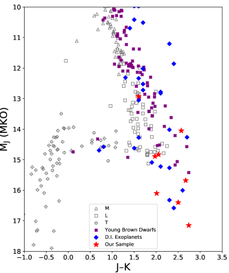
Figure 1: A J$-$K color-magnitude diagram showing the difference in the near-IR color of older field dwarfs (Dupuy & Liu, 2012), and young objects. Included are young brown dwarfs from the UltracoolSheet (Best et al., 2020), directly imaged exoplanets from the NASA Exoplanet Archive, and our sample.

We obtained $L$-band spectra of seven of these young brown dwarfs between 2014 October 27 and December 8 using the Gemini Near-InfraRed Spectrograph (GNIRS; Elias et al., 2006) at the Gemini North Observatory on Maunakea. Details of our observations are listed in Table 2. For these seven objects, we used the 10.44 lines mm^$-$1 grating with the 0$\aas@@fstack{\prime\prime}$05 pix^–1 camera resulting in a continuous 2.98–3.96 $\mu$m spectrum. For most of our targets, we used a slit with a 0$\aas@@fstack{\prime\prime}$3 width, resulting in a spectral resolving power ($R={\lambda}/{\Delta\lambda}$) varying linearly with wavelength from $\sim$500 at 2.98 $\mu$m to $\sim$675 at 3.96 $\mu$m with an average of $R\approx 590$. For our two faintest targets, we used a 0$\aas@@fstack{\prime\prime}$6750-wide slit, resulting in $R\sim$225 to $\sim$300 from 2.98 to 3.96 $\mu$m with an average of $R\approx 260$. For our science target observations, we used a maximum exposure time of 10 sec and 5 sec for observations taken with the 0$\aas@@fstack{\prime\prime}$3 and 0$\aas@@fstack{\prime\prime}$675 slits respectively, and took 10–60 coadds to reach the integration times listed in Table 2. An ABBA nodding pattern was used to enable dark, bias, and sky subtraction. Observations of telluric standard stars with spectral types ranging from B9 V to A0.5V were taken adjacent to observations of our targets.

Our sample also includes 2MASS J22443167+2043433, a young brown dwarf with a published $L$-band spectrum (3.0$-$4.1 $\mu$m, $R\approx$ 460; Stephens et al., 2009) obtained with the Gemini Near-InfraRed Imager and Spectrograph (NIRI: Hodapp et al., 2003).

Table 2: GNIRS Observations

Name	Date	Slit	N $\times$ Int. Time	Telluric Standard	$\Delta$ Airmass
	(UT)	(arcsec)	(sec)
2MASS 0045+16	2014 Nov 28	0.300	8$\times$120	HIP 117927	0.025
WISE 0047+68	2014 Nov 30	0.300	8$\times$300	HIP 8016	0.080
2MASS 0103+19	2014 Nov 25	0.675	8$\times$300	HIP 117927	0.076
2MASS 0103+19	2014 Dec 01	0.675	8$\times$300	HIP 117927	0.043
2MASS 0355+11	2014 Oct 27	0.300	8$\times$100	HIP 18907	0.013
2MASS 0501$-$00	2014 Oct 27	0.300	8$\times$300	HIP 24607	0.028
2MASS 0501$-$00	2014 Dec 08	0.300	8$\times$300	HIP 24607	0.185
G 196$-$3B	2014 Dec 08	0.300	8$\times$300	HIP 51697	0.164
PSO 318.5$-$22	2014 Nov 28	0.675	10$\times$300	HIP 108542	0.131
PSO 318.5$-$22	2014 Nov 30	0.675	12$\times$300	HIP 108542	0.210

3 Data Reduction

We reduced our data using the REDSPEC package, modified for use with GNIRS. For spatial map creation, we used the spatmap procedure on the bright telluric standard, which allowed us to reorient the spectra (of both the science target and telluric standard) along the detector rows. To create a spectral map and wavelength calibrate our data, we compared sky emission spectra from our telluric standard observations to a model sky emission spectrum.

We found that the brightness of the sky background made fitting individual sky emission lines challenging, and thus chose to fit the entire 2.98–3.96 $\mu$m spectrum simultaneously. We first Gaussian-smoothed the model sky to match our observed spectral resolving power. We then ran both the observed and model sky spectra through a high-pass filter to remove thermal emission. We established a 3rd order polynomial wavelength solution by specifying the wavelengths of four evenly-spaced (in the spectral direction) anchor pixels. We then used IDL’s AMOEBA to iteratively solve for the wavelengths of the anchor pixels that minimize the difference between our observed (with a wavelength solution determined from a 3rd order fit to our four anchor pixels) and model sky emission spectra. This was done for five spatial slices of the observed sky, which allowed us to align each column with a specific wavelength. After creating the spatial and spectral maps, we rectified all raw frames so that the spectral direction ran along image rows and the spatial (along the slit) dimension was aligned with image columns.

A pair of spectra were extracted for each AB pair with the redspec process. This process first collapses the rectified images in the spectral direction to create a spatial profile of the A$-$B subtracted image. We fit a pair of Gaussian curves centered on the positive and negative peaks in the spatial profile. Residual sky background was subtracted by fitting a line (at each spectral column) to regions of the spatial profile containing no object flux. We extracted the spectra by summing the flux within an aperture equal to 1.4$\times$ the FWHM of the Gaussian fit to the spatial profile, as we found that this value provided the highest signal-to-noise ratio. The noise for each pixel in our spectra was determined by tracking Poisson noise contributions throughout the reduction and extraction process.

These extracted spectra were combined using a robust weighted mean in xcombspec (Cushing et al., 2004), and then were corrected for telluric absorption and flux calibrated using the xtellcor package (Vacca et al., 2003). Though our telluric correction is excellent overall, we removed regions of the spectra where atmospheric transmission is modeled to fall below 20%, as the signal-to-noise ratio in these regions is low and the telluric correction less reliable. This consists of the region around the 3.3 $\mu$m $Q$-branch of methane. Three of our targets had spectra taken on two separate nights. We reduced each night’s data individually, and then combined the final telluric-corrected spectra using xcombspec with a weighted mean.

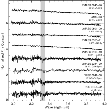
Figure 2: The reduced $L$-band spectra of our objects, normalized and offset to the dotted line. The highlighted region marks the $Q$-branch of methane which appears in our objects at a spectral type of L6. The gap in our spectra are cuts made where atmospheric transmission is below 20% and our telluric correction is less reliable.

We calibrated the absolute flux our spectra using published Spitzer/IRAC Channel 1 (3.6 $\mu$m) photometry (Table 6 in Appendix A), as the IRAC Channel 1 bandpass sits comfortably inside the spectral range of our GNIRS observations. PSO 318.5$-$22 does not have a [3.6] magnitude, so we used its spectral types, WISE W1 magnitudes (Allers & Liu, 2013; Liu et al., 2013) and a spectral type vs. W1$-$[3.6] color relation to compute a [3.6] magnitude of $12.892\pm 0.035$ mags for PSO 318.5$-$22. The spectral type vs. W1$-$[3.6] color relation was created from a linear least-squares fit to the values for young L dwarfs listed in Table 6, which includes some previously unpublished photometry. The photometry, fit, and covariance matrix for the fit can be found in Appendix A. With these [3.6] magnitudes and the zero-magnitude flux for [3.6], we were able to calculate the scaling factor needed to convert our spectra to absolute units of $\mathrm{W~{}m}^{-2}~{}\mu\mathrm{m}^{-1}$ using the process found in Reach et al. (2005). Our final reduced spectra are presented in Figure 2.

4 Analysis

4.1 The Young, L-band Spectral Sequence

In general, the $L$-band spectra of our targets do not show the deep atomic and molecular absorption features that are prominent in near-IR spectra of brown dwarfs (e.g. Kirkpatrick, 2005; Martin et al., 2017). There are some weak water features around 3.0-3.2 $\mu$m, but the strongest absorption feature observed in our spectra is the $Q$-branch of the $\nu_{3}$ fundamental band of methane at 3.3 $\mu$m, and only in our objects of spectral types L6 or later. Moving later in spectral type also corresponds with the spectrum getting redder, shifting from a slightly negative slope with respect to wavelength at L2 to a nearly flat spectrum at L7 when using units of $f_{\lambda}$ (Figure 2). This reddening, along with the onset of methane occurring somewhere between L3 and L6, is consistent with tendencies observed in the spectra of older field dwarfs (Noll et al., 2000; Cushing et al., 2008; Johnston et al., 2019).

4.2 Model Comparisons: Best-Fit Parameters

Fitting spectra to the predictions of atmospheric models has long been a fruitful method for illuminating the physical and chemical processes that occurs in stellar and substellar atmospheres (e.g. Rice et al., 2010). Unfortunately, the medium resolution $L$-band spectra of L dwarfs lack deep features (excluding the $Q$-branch of methane), so a broad range of model parameters have been shown to give statistically good fits when fitting just the $L$-band spectra alone (e.g. Cushing et al., 2008). As such, we chose to combine our $L$-band spectra with the published near-IR spectra listed in Table 3, and then fit both the combined spectrum and just the near-IR spectra in order to gauge how the addition of the $L$-band spectra affects the best-fit parameters for young L dwarfs.

Table 3: IRTF/SpeX Near-IR Spectra

Name	Wavelength	$<{\lambda}/{\Delta\lambda}>$	References
	Range ($\mu$m)
2MASS J0045+16	0.939$-$2.425	750	Allers & Liu (2013)
WISEP J0047+68	0.643$-$2.550	120	Gizis et al. (2012)
2MASSI J0103+19	0.659$-$2.565	120	Cruz et al. (2004)
2MASS J0355+11	0.735$-$2.517	120	Faherty et al. (2013)
2MASS J0501$-$00	0.850$-$2.502	120	Allers et al. (2010)
G 196$-$3B	0.644$-$2.554	120	Allers et al. (2010)
PSO J318.5$-$22	0.646$-$2.553	100	Faherty et al. (2013)
2MASS J2244+20	0.651$-$2.564	100	Looper et al. (2008)

To combine the $L$-band and near-IR spectra, we performed an absolute flux calibration on the near-IR spectra using 2MASS $J$,$H$, and $K_{S}$ photometry (Cutri et al., 2003) with the zero-point fluxes from Cohen et al. (2003). We determined the scaling factor necessary to convert the spectra to units of $\mathrm{W~{}m}^{-2}~{}\mu\mathrm{m}^{-1}$ for each of the three filters, and then used the weighted average of those factors to scale and stitch the near-IR to the $L$ band. PSO 318.5$-$22 lacked 2MASS photometry, so we used MKO $J$,$H$, and $K$ band photometry (Liu et al., 2013), with the zero-points coming from Tokunaga & Vacca (2005). The average percent difference between the three values and the weighted mean was always under 5%, and often under 1%.

Several grids of atmospheric models were used, allowing us to compare how various approaches to 1-D atmospheric models fare. The models we included were:

• BT-Settl CIFIST and BT-Settl AGSS Models (Allard et al., 2012): These models include clouds simulated via detailed dust micro-physics, and an estimation of the diffusion process based on 2D hydrodynamic simulations. These models are in chemical equilibrium, though two different chemical abundances were used for AGSS09 and CIFIST11 (Asplund et al., 2009; Caffau et al., 2011, respectively).

  AGSS Parameter ranges: $T_{\mathrm{eff}}$ ranges from 1000–2600 K at 100 K intervals, log $g$ from 3.5–5.5 [cm/s²] at 0.5 dex intervals, and [Fe/H] = 0.0. Above 2000 K, log $g$ extends to $-$0.5, and [Fe/H] ranges from +0.5 to $-$4 in 0.5 dex increments, and includes [Fe/H] = +0.3.

  CIFIST Parameter ranges: $T_{\mathrm{eff}}$ ranges from 1000–2900 K at 50 K intervals, log $g$ from 3.5–5.5 [cm/s²] at 0.5 dex intervals, and [Fe/H] = 0.0.

• Tremblin Models (Tremblin et al., 2017): These models do not include clouds, instead recreating the effects attributed to clouds by changing the adiabatic index in the layer above the convective zone, artificially heating this portion of the atmosphere and simulating convective fingering. They also include a $K_{\mathrm{zz}}$ mixing parameter that keeps the model from coming to chemical equilibrium. A higher $K_{\mathrm{zz}}$ value models more vigorous mixing.

  Parameter ranges: $T_{\mathrm{eff}}$ ranges from 1200–2400 K at 200 K intervals, all with log $g$ = 3.5 [cm/s²], log $K_{\mathrm{zz}}$ = 6 [$\mathrm{cm}^{2}\mathrm{s}^{-1}$], [Fe/H] = 0.0, and an effective adiabatic index ($\gamma$) of 1.03. We also included 4 models that had already been made for the near-IR fits of specific objects (P. Tremblin, private communication), including two from our sample: PSO 318.5$-$22 ($T_{\mathrm{eff}}$ = 1275 K , log $g$ = 3.7 [cm/s²], log $K_{\mathrm{zz}}$ = 5 [$\mathrm{cm}^{2}\mathrm{s}^{-1}$], [Fe/H] = +0.4, and an $\gamma$ of 1.03) and 2MASS 0355+11 ($T_{\mathrm{eff}}$ = 1400 K, log $g$ = 3.5 [cm/s²], log $K_{\mathrm{zz}}$ = 6 [$\mathrm{cm}^{2}\mathrm{s}^{-1}$], [Fe/H] = +0.2, and an $\gamma$ of 1.01).

• Saumon & Marley Models (Saumon & Marley, 2008): These models account for clouds using an $f_{\mathrm{sed}}$ parameterization, which describes the efficiency of sedimentation in comparison to turbulent mixing, with a lower $f_{\mathrm{sed}}$ value implying thicker clouds. The Saumon & Marley models also include a $K_{\mathrm{zz}}$ mixing parameter to account for disequilibrium chemistry, with a higher $K_{\mathrm{zz}}$ once again modeling more vigorous mixing.

  Parameter ranges: $T_{\mathrm{eff}}$ ranges from 700–2400 K at 100 K intervals, and down to 500 K at 50 K intervals, log $g$ ranges from 4.5–5.5 [cm/s²] at approximately 0.5 dex intervals, with log $K_{\mathrm{zz}}$ of 0, 2, 4 and 6 [$\mathrm{cm}^{2}\mathrm{s}^{-1}$], [Fe/H] = 0.0, and $f_{\mathrm{sed}}$ of 1, 2, 3, and 4, along with a cloud-free model (nc). Additionally, there were cloud-free models with [Fe/H] = +0.3 and +0.5 for 500–600 K, as well as log $g$ of 5.25 [cm/s²] from 500–700 K and 4.0 [cm/s²] from 1500–1700 K. From 800–1500 K, the $f_{\mathrm{sed}}$ = 1 and 2 models included a log $g$ of 4.0, and 4.25 [cm/s²], and the $f_{\mathrm{sed}}$ = 2 models include a log $g$ of 4.75 [cm/s²].

• Drift-Phoenix Models (Witte et al., 2009): These models simulate clouds using detailed dust micro-physics, with a more robust focus on both the seeding and subsequent growth of these cloud-forming grains, and are allowed to come into chemical equilibrium.

  Parameter ranges: $T_{\mathrm{eff}}$ ranges from 1000–2200 K at 100 K intervals, log $g$ from 3.5–5.5 [cm/s²] at 0.5 dex intervals, and [Fe/H] = 0.0.

• Madhusudhan Models (Madhusudhan et al., 2011): These models include clouds which are parameterized by variable dust grain sizes and various upper altitude cutoffs ranging from a sharp cutoff (E) to extending fully to the top of the atmosphere (A), with AE and AEE ranging between the two. The models are also in chemical equilibrium.

  Parameter ranges: $T_{\mathrm{eff}}$ ranges from 700–1700 K at 100 K intervals, log $g$ = 4.0 [cm/s²], with [Fe/H] of 0.0 and +0.5, and dust grain sizes of 30, 60, and 100 $\mu$m. The AE cloud set has some finer $T_{\mathrm{eff}}$ and log $g$ spacing, with a 25 K interval from 750–1050 K and log $g$ ranging from 3.75–4.25 [cm/s²] with a 0.25 dex interval across the whole range.

We found the best fits by first calculating the scaling factor $C$ (where $C$ has the physical analog [Radius²/Distance²]) that minimized $G_{\mathrm{k}}$, a goodness-of-fit statistic (Cushing et al., 2008), for each model spectrum. Then for each model set the synthetic spectrum with the minimum $G_{\mathrm{k}}$ is selected as the best-fit model. We report the parameters of these models, for both the near-IR and combined spectra, in Table 4.2.3.

For the sake of compactness, PSO 318.5$-$22 and 2MASS 0355+11 are presented as a representative sample for the rest of the paper, with PSO 318.5$-$22 representing the cooler and later spectral types and 2MASS 0355+11 the hotter and earlier. The best near-IR fits of 2MASS 0355+11 and PSO 318.5$-$22 can be seen in Figures 3 and 4, respectively. Note that the $L$-band spectra is included in these figures, but not in this fitting process. The combined best fits for these objects can be seen in Figures 5 and 6, respectively. The combined fits for the remaining objects can be found in Appendix B.

When we calculate the best fits to just the published near-IR spectra of our sample, we find that the models fit portions of the near-IR well, though there are definitely a variety of deviations for each set of models, which matches what was seen for young brown dwarfs in Manjavacas et al. (2014). However, 8 of the 12 fits are very poor matches to the the $L$ band, as can be seen in Figures 3 and 4. The BT-Settl CIFIST and Tremblin models fit the $L$ band well enough for hotter objects like 2MASS 0355+11, but underestimate the $L$-band flux at lower temperatures. Similarly, the Saumon & Marley models provide one of the better $L$-band fits for PSO 318.5$-$22, but for the hotter objects they predict strong water features in the $L$ band that are not present. For these same hotter objects the Drift-Phoenix best-fit models predict too much flux emerging out of the $L$ band. Between $T_{\mathrm{eff}}$ of 1600 K and 1400 K the Drift-Phoenix models transition from being bright in the $J$ and $H$ bands to bright in $K$ and $L$ bands (This transition can be seen between Figures 3, 5, and 9 which show the 1500, 1600, and 1400 K models respectively). This rapid reddening causes most of the cooler objects to be fit by the Drift-Phoenix models at either 1600 or 1500 K, and leads to Drift-Phoenix having the best $L$-band fit of PSO 318.5$-$22, even though the near-IR fit is the worst. All of these discrepancies show that a reasonable fit at near-IR wavelengths does not necessarily mean the same model spectra will also fit the $L$-band region well.

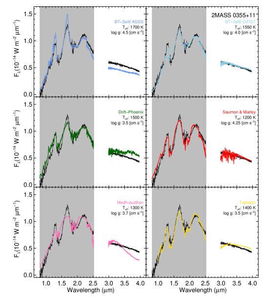
Figure 3: The combined spectrum of 2MASS 0355+11 (black) compared to the model spectra (colored) with parameters that best fit only the shaded near-IR portion of the spectrum.

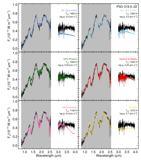
Figure 4: Same as Fig. 3, except using the cooler PSO 318.5$-$22.

4.2.1 Overall Summary of the Combined Fits

When we fit to the combined spectra (See Figures 5 and 6 and Appendix B) we find that no single model set fits all the objects well. The Saumon & Marley and Tremblin models are the most consistent across the whole spectral range, and the best fits for the later spectral types. For the earlier types, the BT-Settl CIFIST models are often better, but these best-fit models for the later type objects have muted $J$, $H$, and $K$ peaks and shallower troughs between peaks as seen in Figure 6. The Drift-Phoenix models tend to fit the $L$ band fairly well, particularly the flux levels between the near-IR and $L$ band, yet the fit to the near-IR is not good. Figure 6 is a good example of both the flux level match and the near-IR mismatch. The Madhusudhan and BT-Settl AGSS models are not the best fitting model for any of our objects’ combined spectra. The Madhusudhan models’ poor fits are caused by a humped $L$ band, as well as under-predicting the flux emerging from the $J$ and $H$ bands, which can be seen in both Figures 5 and 6. For the BT-Settl AGSS models, the poor fits are due to the fact that when the flux levels between the near-IR and $L$-band match the observed spectra, the near-IR spectral morphology is off as seen in Figure 5 (often bright in the $K$ band and dim in the $J$ band).

4.2.2 Temperature

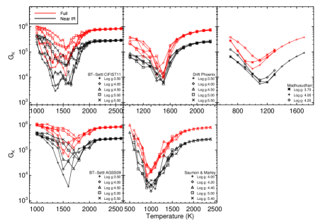
Figure 7: The goodness-of-fit parameter ($G_{\mathrm{k}}$) for PSO 318.5$-$22 plotted as function of temperature and log $g$. Note that the shape does not change drastically when including the $L$ band, but it does move to cooler temperatures ($\sim$100 K). This held true across all of our objects.

When we calculate the best fits for the combined spectra, we find the best-fit temperatures are generally $\sim$100 K colder compared to the fits to just the near-IR, as seen in Table 4.2.3. The lower temperature of fits that include the $L$ band can be also seen in Figure 7, which compares the $G_{\mathrm{k}}$ values for PSO 318.5$-$22 for a range of model temperatures and surface gravities. The shape of the $G_{\mathrm{k}}$ plots for temperature and surface gravity are similar for both the combined and near-IR spectra but including the $L$ band offsets the curve to colder temperatures. This temperature drop is caused in part by the higher temperature models under-predicting the flux ratio between the near-IR and the $L$ band. Even cases where a model’s best-fit temperature increased by adding the $L$ band had this 100 K shift (for example the BT-Settl CIFIST fit of PSO 318.5$-$22). In these cases there are two local minima: the hotter minimum with muted troughs and peaks in the near-IR, while the cooler one is less muted. For both cases, the minima shift to cooler temperatures when the $L$ band is added, but the absolute minima switches from the colder minima to the hotter one.

The combined best-fit temperatures also divides our models into two groups: those models that generally give higher temperature fits for our objects (BT-Settl and Drift-Phoenix) and those that fit these same objects with lower temperatures (Madhusudhan, Tremblin, and Saumon & Marley). The colder-model fits all share a similar feature in their $P/T$ profile: Moving radially outward, they track with similar models until at some height they have a sharp decrease in pressure over a small temperature range, after which they continue along similar models except with hotter temperatures in the upper layers of the atmosphere (Madhusudhan et al., 2011, Examples can bee seen in Fig. 3 inTremblin et al., 2016, , Fig. 4 inMarley et al., 2010, , and Fig. 1 in). The cause of this thermal perturbation is not the same for all models, as the modified adiabatic index produces the perturbation in the Tremblin models while the existence of clouds produces it in the Madhusudhan and Saumon & Marley models. It should be noted that not all the Madhusudhan and Saumon & Marley models have this thermal perturbation, only the ones with thick clouds (Type A for Madhusudhan, and at lower $f_{\mathrm{sed}}$values for Saumon & Marley).

4.2.3 Clouds

Two of the model grids allow us to also look at the effects of variations in cloud properties. For both sets of models the thickest clouds were consistently the best fits (the $f_{\mathrm{sed}}$ of 1 for Saumon & Marley and cloud type A for Madhusudhan), and with the fits getting progressively worse for thinner clouds. Thick clouds cause an increase in opacity which blocks flux coming from the deeper and hotter layers of the atmosphere. As such, the near-IR, which originates below the added cloud deck in cloudless models, is now emerging from a cooler region just above the cloud deck instead. (Ackerman & Marley, 2001). Now that less flux is coming out in the near-IR, to maintain a level of radiation consistent with the $T_{\mathrm{eff}}$ of this object the upper atmosphere must heat up. Since the $L$ band originates from these upper layers, we get an increase in $L$ band flux, which when combined with the lower near-IR flux results in better fits. However, the thick clouds (combined with a high $K_{\mathrm{zz}}$ for Saumon & Marley) also create a turndown at the long end of the $L$ band that we do not see in our data. This can be seen in Figure 6, and is also an issue for several of the other models. Still, overall it seems that if clouds are the answer to the spectral reddening of our young objects as suggested by Manjavacas et al. (2014) and Faherty et al. (2016), then they will need to be thick rather than thin to best fit the full spectrum.

Table 4: Atmospheric Model Fits

Model	Best Fit to Near-IR only							Best Fit to Near-IR + $L$ Band
	$T_{\mathrm{eff}}$	log $g$	[Fe/H]	$f_{\mathrm{sed}}$	$K_{\mathrm{zz}}$	Dust Size	$G_{\mathrm{k}}$	$T_{\mathrm{eff}}$	log $g$	[Fe/H]	$f_{\mathrm{sed}}$	$K_{\mathrm{zz}}$	Dust Size	$G_{\mathrm{k}}$
	(K)	[cm/s2]			[$\mathrm{cm}^{2}\mathrm{s}^{-1}$]	($\mu$m)		(K)	[cm/s2]			[$\mathrm{cm}^{2}\mathrm{s}^{-1}$]	($\mu$m)
2MASS 0045+16:
BT-Settl AGSS09	2000	4.50	+0.5				253710	2000	5.00	+0.5				493972
BT-Settl CIFIST11	1800	5.00	0.0				184374	1800	5.00	0.0				202512
Drift-Phoenix	1700	4.00	0.0				217628	1800	4.50	0.0				359250
Saumon & Marley	1600	4.48	0.0	1	6		174446	1600	4.48	0.0	1	6		231808
Madhusudhan	1700	4.0	0.0			100	485212	1700	4.0	0.0			100	612891
Tremblin	2000	3.5	0.0		6		174357	2000	3.5	0.0		6		366177
G196$-$3B:
BT-Settl AGSS09	1700	3.50	0.0				15589	1700	4.50	0.0				42102
BT-Settl CIFIST11	1750	4.00	0.0				14745	1700	3.50	0.0				40166
Drift-Phoenix	1600	4.50	0.0				28231	1600	4.00	0.0				43899
Saumon & Marley	1400	4.25	0.0	1	4		21832	1400	4.25	0.0	1	4		49006
Madhusudhan	1400	4.0	0.0			60	47408	1400	4.0	0.0			100	103123
Tremblin	1600	3.5	0.0		6		15486	1600	3.5	0.0		6		23985
2MASS 0501$-$00:
BT-Settl AGSS09	2000	5.50	+0.5				23214	1700	4.50	0.0				105845
BT-Settl CIFIST11	1650	5.00	0.0				18834	1600	5.00	0.0				106892
Drift-Phoenix	1600	3.50	0.0				18862	1600	3.50	0.0				35401
Saumon & Marley	1400	4.00	0.0	1	6		15106	1400	4.25	0.0	1	4		106145
Madhusudhan	1500	4.0	0.0			60	53237	1400	4.0	0.0			100	222405
Tremblin	1800	3.5	0.0		6		12864	1600	3.5	0.0		6		70538
2MASS 0355+11:
BT-Settl AGSS09	1700	4.50	0.0				13796	1600	3.50	0.0				75661
BT-Settl CIFIST11	1550	4.00	0.0				5305	1550	4.00	0.0				21312
Drift-Phoenix	1500	3.50	0.0				11847	1600	5.00	0.0				94024
Saumon & Marley	1200	4.25	0.0	1	6		12298	1200	5.47	0.0	1	4		77846
Madhusudhan	1300	3.75	0.0			60	17793	1200	4.25	0.0			60	187057
Tremblin	1400	3.5	+0.2		6		7631	1400	3.5	0.0		6		67283
2MASS 0103+19:
BT-Settl AGSS09	1500	4.50	0.0				5615	1700	4.50	0.0				24475
BT-Settl CIFIST11	1650	5.00	0.0				2912	1500	5.00	0.0				15322
Drift-Phoenix	1600	3.50	0.0				4581	1600	4.50	0.0				11271
Saumon & Marley	1400	4.25	0.0	1	6		2551	1300	4.00	0.0	1	2		17097
Madhusudhan	1400	4.0	0.0			60	7222	1300	4.0	0.0			100	28273
Tremblin	1800	3.5	0.0		6		4101	1600	3.5	0.0		6		17127
2MASS 2244+20:
BT-Settl AGSS09	1700	4.50	0.0				47015	1600	3.50	0.0				109410
BT-Settl CIFIST11	1400	4.50	0.0				25443	1400	4.00	0.0				58998
Drift-Phoenix	1500	3.50	0.0				47917	1500	3.50	0.0				63373
Saumon & Marley	1200	4.00	0.0	1	4		10359	1000	4.00	0.0	1	6		27231
Madhusudhan	1300	4.0	0.0			60	44486	1200	4.0	0.0			60	78465
Tremblin	1400	3.5	+0.2		6		15470	1400	3.5	+0.2		6		40499
PSO 318.5$-$22:
BT-Settl AGSS09	1600	3.50	0.0				3633	1600	3.50	0.0				54994
BT-Settl CIFIST11	1350	3.50	0.0				2861	1550	3.50	0.0				11876
Drift-Phoenix	1500	5.00	0.0				5423	1500	5.00	0.0				9482
Saumon & Marley	1000	4.25	0.0	1	6		2122	900	5.00	0.0	1	4		8704
Madhusudhan	1100	4.0	0.0			30	5440	1000	4.0	+0.5			60	21581
Tremblin	1275	3.7	+0.4		5		1694	1200	3.5	0.0		6		12564
WISE 0047+68:
BT-Settl AGSS09	1700	4.50	0.0				23472	1600	3.50	0.0				131724
BT-Settl CIFIST11	1400	4.00	0.0				13212	1500	3.50	0.0				57278
Drift-Phoenix	1500	3.50	0.0				25152	1500	4.00	0.0				47773
Saumon & Marley	1100	4.47	0.0	1	6		5711	1000	4.00	0.0	1	6		20615
Madhusudhan	1200	4.25	0.0			60	19659	1100	4.0	+0.5			100	76802
Tremblin	1400	3.5	+0.2		6		5935	1275	3.7	+0.4		5		25983

References. — (A16) Allers et al. (2016), (AL13) Allers & Liu (2013), (C09) Cruz et al. (2009), (F12) Faherty et al. (2012), (F13) Faherty et al. (2013), (F16) Faherty et al. (2016), (G15) Gizis et al. (2015), (K08) Kirkpatrick et al. (2008), (L16) Liu et al. (2016), (L13) Liu et al. (2013), (V18) Vos et al. (2018)

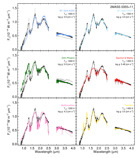
Figure 5: The combined spectrum of 2MASS 0355+11 (black) compared to the model spectra (colored) with parameters that best fits the entire combined spectrum. For ease of comparison, the near-IR best-fit models are shown in grey.

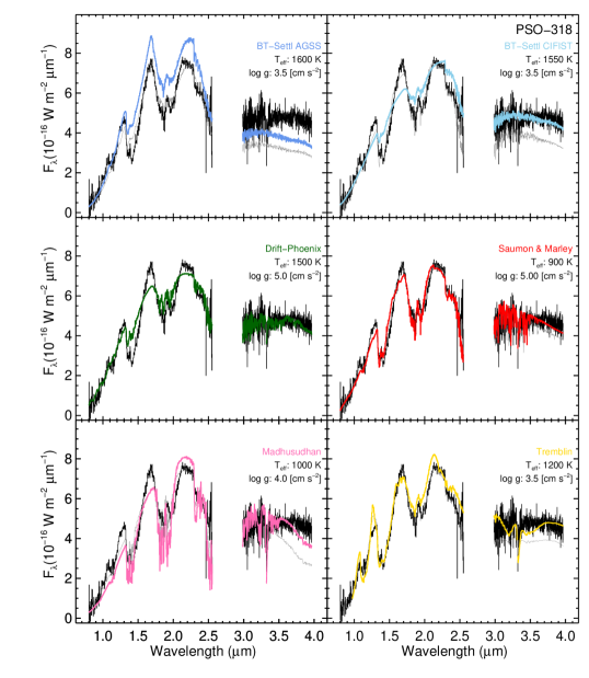
Figure 6: Same as Figure 5, except using the cooler PSO 318.5$-$22

4.2.4 Mixing Rate

We can see how the vertical mixing rate ($K_{\mathrm{zz}}$) tends to vary with the inclusion of the $L$ band through the Saumon & Marley fits. With the inclusion of the $L$-band spectra, there is a shift to lower $K_{\mathrm{zz}}$ values (from the max possible 6 [$\mathrm{cm}^{2}\mathrm{s}^{-1}$] to 4 or even 2) for the combined spectra, which on face value disagrees with the conclusions from Miles et al. (2018) finding a need for a high $K_{\mathrm{zz}}$ (around $10^{8}$ $\mathrm{cm}^{2}\mathrm{s}^{-1}$) to explain $L$-band features. However, when the models’ thickest cloud parameter was used (f1), as was the case in the best fit for all of our objects, changing the log $K_{\mathrm{zz}}$ value from 6 to 4 had little affect on the model spectra in the near-IR and $L$ band. The effect on $G_{\mathrm{k}}$ was at its highest a 0.5 percent increase, and sometimes was as small as 0.01 percent. For some temperatures, the insensitivity of the model to $K_{\mathrm{zz}}$ extends down to $K_{\mathrm{zz}}$ of 2 [$\mathrm{cm}^{2}\mathrm{s}^{-1}$], like at the best-fit temperature of 2MASS 0103+19 (1300 K), but often the lowered vertical mixing would start to deepen the $L$-band methane features at this point, making the fit noticeably worse. When a thinner cloud parameter was set, the best-fit $K_{\mathrm{zz}}$ values tended to stay high. Overall, we have a low sensitivity between the higher $K_{\mathrm{zz}}$ values, but can still say we agree with Miles et al. (2018) that higher values in general create better fits.

4.3 Model Comparisons: Evolutionary Parameters

Some of our objects are members of young moving groups and therefore have ages associated with them. These ages, along with measured $L_{\mathrm{bol}}$ and evolutionary models, give well-defined evolutionary parameters for five of our objects, 2MASS 0045+16, 2MASS 2244+20, WISE 0047+68, 2MASS 0355+11 (All from Faherty et al., 2016) and PSO 318.5$-$22 (Allers et al., 2016). The memberships, ages, masses, effective temperature, and surface gravities for all of these objects can be found in Table 5. We can us these $T_{\mathrm{eff}}$ and log $g$ values to select synthetic spectra that match these parameters, which we’ll hereafter refer to as evolutionary effective temperature and surface gravity. For each model set, we took the model spectrum with the effective temperature and surface gravity closest to each object’s evolutionary effective temperature and surface gravity, and of these selected the model parameters and $C$ which minimized $G_{\mathrm{k}}$. The Madhusudhan and Tremblin models do not fully cover the range of temperatures and gravities needed to encompass all of the objects evolutionary temperatures and gravities. When this occurred, the closest available parameters were used. The comparisons for these objects can be seen in Figures 8 through 12. For ease of reference, the combined best-fit model from the previous section is also plotted in grey.

Table 5: Our Sample of Young L Dwarfs With Known Moving Groups and Ages

Name	YMG	Age	Mass Range	$T_{\mathrm{eff}}$	log $g$	Refs
	Membership	(Myrs)	($M_{\mathrm{Jup}}$)	(K)	[$\mathrm{cm}^{2}\mathrm{s}^{-1}$]
2MASS J0045+16	Argus	40	20–29	$2059\pm 45$	$4.22\pm 0.10$	C09, F15, L16, F16
2MASS J0355+11	AB Dor	110–130	15–27	$1478\pm 58$	$4.58^{+0.07}_{-0.17}$	C09, F13, AL13, F16
WISEP J0047+68	AB Dor	110–130	9–15	$1230\pm 27$	$4.21\pm 0.10$	G15, F15 ,F16
2MASS J2244+20	AB Dor	110–130	9–12	$1184\pm 10$	$4.18\pm 0.08$	K08, F15, A16
PSO J318.5$-$22	$\beta$ Pic	20–26	5–7	$1127^{+24}_{-26}$	4.01 $\pm$ 0.03	L13, A16, F16

For all our objects except 2MASS 0045+16, we see that the Drift-Phoenix and the BT-Settl AGSS models do not fit well when the evolutionary effective temperature and surface gravity are used. The Drift-Phoenix model over-predicts the flux in the $L$ band, with the peaks of the $J$ and $H$ bands being almost non-existent, which can be most clearly seen in Figure 11. The AGSS model has the opposite problem, as already at 1400 K in Figure 9 it looks remarkably like a T dwarf with its deep methane absorption in the near-IR and $L$ band. The fact that the methane absorption is this strong in the AGSS model at such high temperatures is part of why the best-fit temperatures were hot for our young L dwarfs. The exception is our hottest object 2MASS 0045+16 (Figure 8), which the AGSS model arguably has the best fit. Meanwhile, the Drift-Phoenix model inverts its color with the $J$ and $H$ band being too strong compared to weaker $L$ and $K$ bands, though not quite as dramatically at this temperature.

The CIFIST model set is one of the better fits for 2MASS 0355+11 when using the evolutionary effective temperature and surface gravity, where its biggest issues are predicting stronger water absorption features than we observe, both between the near-IR bands and in the $L$ band, and missing the sharp triangle shape of the H band. This issue is there in all the objects, but it is most pronounced for the colder ones like in Figure 10, where the predicted water absorption becomes even stronger, and is accompanied by strong methane features as well. This increased absorption drops the model’s $L$-band flux level too low. In general, the CIFIST BT-Settl model set seems to do comparatively well for young L dwarfs at higher temperatures, but struggles when transitioning to lower temperatures.

The selected Madhusudhan models have the opposite problem, fitting colder objects better than hotter ones. When using the evolutionary effective temperature and surface gravity of 2MASS 0355+11 and 2MASS 0045+16, we see the differences in the flux levels of the near-IR and $L$ band are much greater in the model than in the observed spectrum. This disparity is not there for the three colder objects, though other issues occur, such as over-estimation of the $K$-band flux and a turndown at the long end of the $L$ band. However, these issues are minor compared to the flux level spread between the bands at higher temperatures, which explains the Madhusudhan model’s tendency to give colder best-fit temperatures.

The Tremblin and Saumon & Marley model sets are the most consistently good fits, though both still have some discrepancies. The Saumon & Marley models tend to overestimate the flux in the $J$ and $H$ bands, especially for the 2MASS 0045+16 and 2MASS 0035+11. Models with lower temperatures have lower near-IR flux which are closer to the observed values, such as in Figure 10, which explains why the models’ best fits trend towards colder temperatures. The Tremblin models are off in the near-IR about as much as the Saumon & Marley models, but with no consistent issues. For the three coldest objects, the Tremblin models matches the $L$-band flux level, yet exhibits strong absorption in the $P$, $Q$, and $R$ branches of methane unseen in the observed spectrum. Both also under-predict the $L$-band flux for 2MASS 0045+16, though this is consistent across all the models.

Looking more generally, the three of the four models without disequilibrium chemistry (both BT-Settl models and Drift-Phoenix) show an onset of methane at higher temperatures than we observe, such as in Figure 9. This agrees with what we saw from the best-fit models. This effect is especially notable in the BT-Settl AGSS models, whose spectra at this temperature look more similar to T dwarfs than L dwarfs. The Madhusudhan model with the thickest clouds (Type A) does not have this early appearance of methane, but the less thick AE clouds do, with $Q$-band absorption being strong even at 1400 K. As for the models with disequilibrium chemistry, the $Q$-branch of methane is well fit when using the evolutionary effective temperature and surface gravity, and overall are generally the better fit compared to the equilibrium models. We also find that the cloudless BT-Settl models clouds tend to fit the colder objects worse than those with clouds as their evolutionary temperature, as seen in Figures 10-12. The exception to the cloudy models fitting better is the Drift-Phoenix models, which are poor past 1500 K due to so little flux coming out in the $J$ and $K$ bands. This is evidence that some combination of clouds and disequilibrium chemistry is a necessary for modeling brown dwarf atmospheres with accurate effective temperatures.

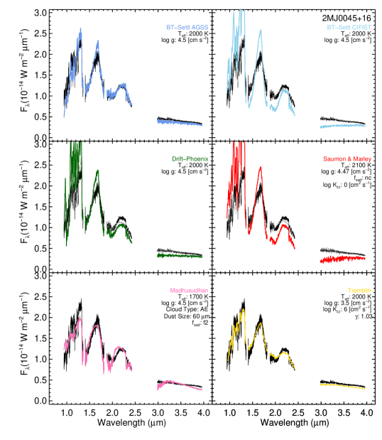
Figure 8: The spectra of 2MASS 0045+16 compared to the spectra from each model set that best matches the known evolutionary effective temperature and surface gravity found in Table 5. Note that in this case the Tremblin models do not extend to 4.5 [$\mathrm{cm}^{2}\mathrm{s}^{-1}$] and the Madhusudhan models do not extend to 2000 K. In gray is also the combined best-fit spectra (in the case of the Tremblin models, the best-fit and evolutionary model parameters are the same).

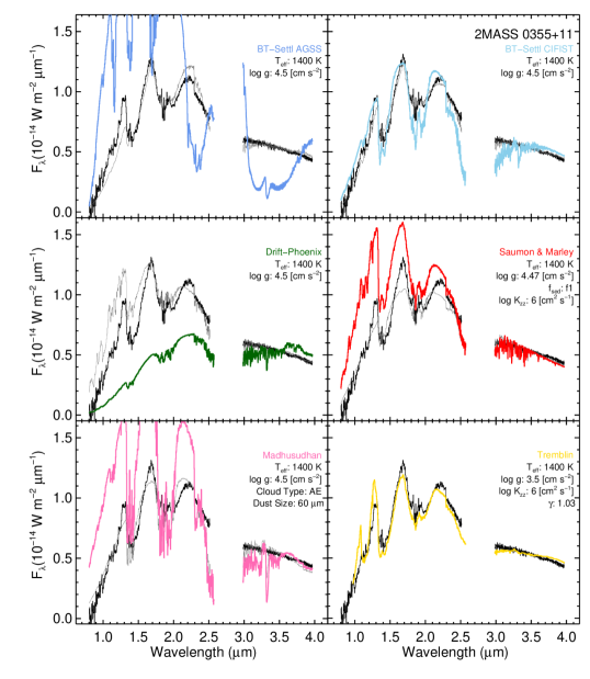
Figure 9: The spectra of 2MASS 0355+11 compared to the spectra from each model set that best matches the known evolutionary effective temperature and surface gravity found in Table 5. Note that in this case the Tremblin models do not extend to 4.5 [$\mathrm{cm}^{2}\mathrm{s}^{-1}$]. In gray is also the combined best-fit spectra (in the case of the Tremblin models, the best-fit and evolutionary model parameters are the same).

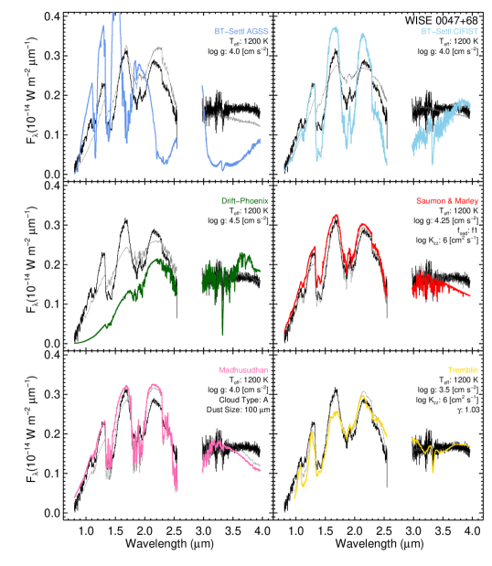
Figure 10: The spectra of WISE 0047+68 compared to the spectra from each model set that best matches the known evolutionary effective temperature and surface gravity found in Table 5. Note that in this case the Tremblin models do not extend to 4.0 [$\mathrm{cm}^{2}\mathrm{s}^{-1}$]. In gray is also the combined best-fit spectra.

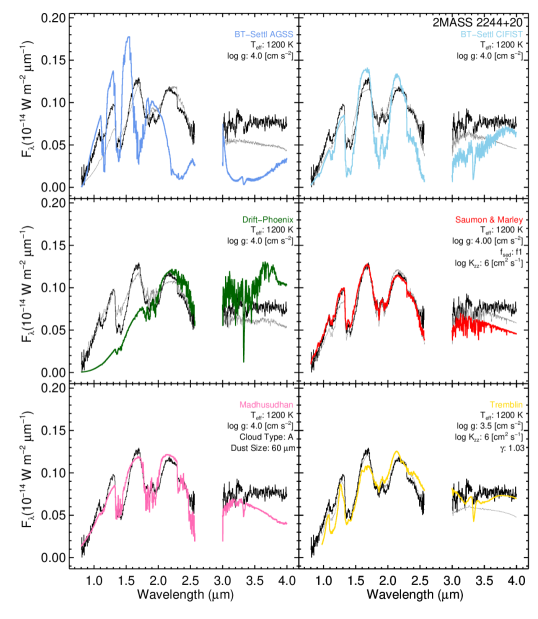
Figure 11: The spectra of 2MASS 2244+20 compared to the spectra from each model set that best matches the known evolutionary effective temperature and surface gravity found in Table 5. Note that in this case the Tremblin models do not extend to 4.0 [$\mathrm{cm}^{2}\mathrm{s}^{-1}$]. In gray is also the combined best-fit spectra (in the case of the Madhusudhan models, the best-fit and evolutionary model parameters are the same).

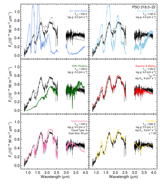
Figure 12: The spectra of PSO 318.5$-$22 compared to the spectra from each model set that best matches the known evolutionary effective temperature and surface gravity found in Table 5. Note that in this case the Tremblin models do not extend to 1100 K or 4.0 [$\mathrm{cm}^{2}\mathrm{s}^{-1}$]. In gray is also the combined best-fit spectra (in the case of the Tremblin models, the best-fit and evolutionary model parameters are the same).

4.4 AB Dor Sub-population

Three of our targets, 2MASS 2244+20, WISE 0047+68, and 2MASS 0355+13, are members of the AB Doradus young moving group, and thus can be assumed to have similar compositions and ages ($\sim$120 Myrs, Barenfeld et al., 2013) due to their shared origin and formation history. WISE 0047+68 and 2MASS 2244+20 have approximately the same mass, respectively 9-15 and 9-12 $M_{\rm{Jup}}$, but 2MASS 0355+13 is almost twice as massive at 15-27 $M_{\rm{Jup}}$. This means Figure 13, which shows the spectra of these three objects, is a mass sequence at a fixed age and composition, though admittedly an abbreviated one. 2MASS 0355+13 is more luminous than WISE 0047+68 and 2MASS 2244+20, whose spectra lie nearly on top of each other due to having similar masses (See Table 5). Of particular interest is the 3.3 $\mu$m $Q$-branch methane feature, which has a similar depth in the two cooler objects, even with different infrared spectral types and gravity classification (WISE 0047+68 as L7 INT-G and 2MASS 2244+20 as L6 VL-G). This feature is absent in the more massive (and hotter) 2MASS 0355+13, showing the temperature dependence of the methane feature for a fixed age and composition. AB Dor has several other ultracool members (Faherty et al., 2016), which means it will be possible to expand this mass sequence.

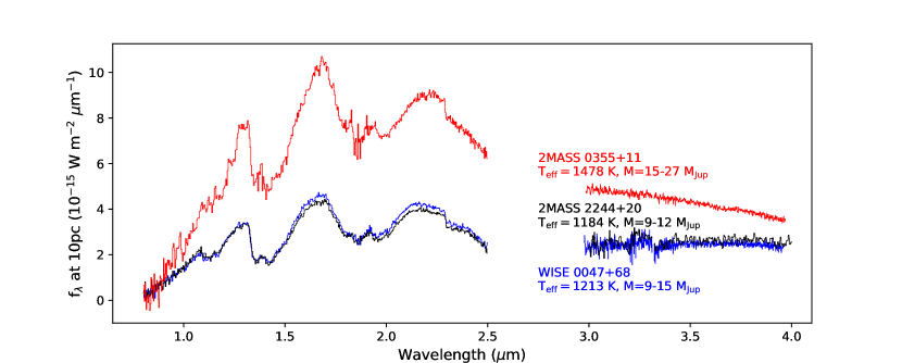
Figure 13: Spectra of three members of the young moving group AB Dor, placed at 10 pc. The two objects of the same mass lie almost on top of each other, and with a $Q$-branch methane feature of similar depth. This feature is absent in the hotter and more massive 2MASS 0355+11.

5 Conclusions

From this work, we can see that $L$-band spectra are not particularly strong diagnostic tools on their own for young L dwarfs due to a lack of strong features (with the exception of the $Q$-branch of methane). However, when used in hand with near-IR spectra it is extremely useful for understanding objects’ atmospheric properties. The inclusion of the $L$ band highlights where models are falling short, and what physical processes models need to include to match observations. We find adding the $L$ band lowers the best-fit effective temperature of our models by $\sim$100 K. For these fits, when clouds are included in the models, thick ones are preferred, and when a vertical mixing rate is used ($K_{\mathrm{zz}}$), higher values give the best results. We also note that for models to fit the combined spectra well at the published evolutionary effective temperatures for these objects, we need models with disequilibrium chemistry and/or clouds. Overall, we find the Tremblin and Saumon & Marley models fit the full spectrum of the young objects best. These results show the power of wide spectral coverage, matching conclusion from Burningham et al. (2021), and we recommend that our data also be used to enhance future retrievals of these objects to parse their diversity. In particular though, these observations show the value of the $L$ band for understanding the atmospheres of young brown dwarfs, and the giant exoplanets for which they act as proxies and give us a preview of the insights that the James Webb Space Telescope will bring.

Data Availability

The combined spectra for all of these objects are available in the online supplementary material for this article.

Appendix A IRAC Channel 1 Photometry

PSO 318.5$-$22 does not have [3.6] magnitudes, so we used its spectral type, W1 magnitude (Allers & Liu, 2013; Liu et al., 2013) and a spectral type vs. W1$-$[3.6] color relation to compute its [3.6] magnitude. The spectral type vs. W1$-$[3.6] color relation was created from a linear least-squares fit to the values for young L dwarfs listed in Table 6. We found the relation to be W1$-$[3.6] = $0.0822*$SpT$+0.015$, where SpT = 10 for a dwarf with a near-IR spectral type of L0, with a covariance matrix of: $\begin{bmatrix}1.18\times 10^{-3}&-8.86\times 10^{-5}\\ -8.86\times 10^{-5}&6.94\times 10^{-6}\end{bmatrix}$

Several of these objects are known low-gravity brown dwarfs which lack published IRAC photometry, but have available IRAC data in the Spitzer Heritage Archive. We computed IRAC Channel 1 photometry from Post-BCD pipeline mosaicked images using the same method as Dupuy & Kraus (2013). We calculated the fluxes in a 3$\aas@@fstack{\prime\prime}$6 radius with a background annulus of 3$\aas@@fstack{\prime\prime}$6-8$\aas@@fstack{\prime\prime}$4. Photometry was performed using the phot routine from IDL Astronomy User’s Library (Landsman, 1996). We applied aperture corrections as recommended by the IRAC data handbook. We determined uncertainties on our aperture photometry using a Monte Carlo approach to account for uncertainties from associated post-BCD uncertainty images. Our final photometric uncertainties also include published uncertainties for aperture corrections and flux zero points. For comparison, we also calculated photometry for the young brown dwarfs in Luhman et al. (2009) and found that our results agree with their published IRAC magnitudes to within our typical error of 0.02-0.03 mags. Table 6 includes IRAC photometry for low-gravity L dwarfs, including objects in our sample.

Table 6: IRAC and WISE photometry of young L dwarfs

Name	SpT	AllWISE	IRAC	Refs.
	Near-IR	W1 (mag)	ch1 (mag)
2MASS J00325584$-$4405058	L0 vl-g	$12.839\pm 0.024$	$12.585\pm 0.017$	This work, Allers & Liu (2013)
WISEP J004701.06+680352.1	L7 int-g	$11.881\pm 0.023$	$11.518\pm 0.017$	This work, Gizis et al. (2015)
2MASS J010332.03+1935361	L6 int-g	$13.177\pm 0.024$	$12.930\pm 0.020$	Metchev et al. (2015), Allers & Liu (2013)
2MASS J01415823$-$4633574	L0 vl-g	$12.584\pm 0.023$	$12.360\pm 0.020$	Luhman et al. (2009), Allers & Liu (2013)
2MASS J02411151$-$0326587	L1 vl-g	$13.649\pm 0.025$	$13.390\pm 0.020$	Luhman et al. (2009), Allers & Liu (2013)
2MASS J03231002$-$4631237	L0 vl-g	$13.091\pm 0.024$	$12.840\pm 0.020$	Luhman et al. (2009), Cruz et al. (2018)
2MASS J03552337+1133437	L3 vl-g	$10.526\pm 0.024$	$10.280\pm 0.017$	This work, Allers & Liu (2013)
2MASS J03572695$-$4417305	L0 int-g	$12.486\pm 0.023$	$12.210\pm 0.020$	Luhman et al. (2009), Cruz et al. (2018)
2MASS J04433761+0002051	L0 vl-g	$10.831\pm 0.023$	$10.550\pm 0.020$	Luhman et al. (2009), Allers & Liu (2013)
2MASS J05012406$-$0010452	L3 vl-g	$12.050\pm 0.023$	$11.770\pm 0.020$	Luhman et al. (2009), Allers & Liu (2013)
2MASSI J0518461$-$275645	L1 vl-g	$13.043\pm 0.023$	$12.797\pm 0.017$	This work, Allers & Liu (2013)
2MASS J06085283$-$2753583	L0 vl-g	$11.975\pm 0.024$	$11.750\pm 0.020$	Luhman et al. (2009), Allers & Liu (2013)
G 196-3B	L-3 vl-g	$11.700\pm 0.023$	$11.660\pm 0.020$	Zapatero Osorio et al. (2010), Allers & Liu (2013)
2MASS J11193254$-$1137466AB	L7 vl-g	$13.548\pm 0.026$	$13.234\pm 0.017$	This work, Kellogg et al. (2016)
WISEA J114724.10$-$204021.3	L7 vl-g	$13.718\pm 0.026$	$13.352\pm 0.017$	This work, Schneider et al. (2016)
2MASSI J1615425+495321	L3 vl-g	$13.212\pm 0.024$	$12.910\pm 0.020$	Luhman et al. (2009), Allers & Liu (2013)
2MASS J17260007+1538190	L3 int-g	$13.067\pm 0.024$	$12.760\pm 0.020$	Luhman et al. (2009), Allers & Liu (2013)
PSO J318.5338$-$22.8603	L7 vl-g	$13.237\pm 0.024$		Liu et al. (2013)
2MASS J2206449$-$421720	L4 vl-g	$12.856\pm 0.023$	$12.560\pm 0.017$	This work, Cruz et al. (2018)
2MASS J22081363+2921215	L3 vl-g	$13.381\pm 0.025$	$13.080\pm 0.020$	L09, Allers & Liu (2013)
2MASS J22134491$-$2136079	L0 vl-g	$13.247\pm 0.026$	$12.990\pm 0.020$	L09, Allers & Liu (2013)
2MASS J22443167+2043433	L6 vl-g	$12.790\pm 0.022$	$12.350\pm 0.020$	Leggett et al. (2007), Allers & Liu (2013)
SDSS J224953.47+004404.6AB	L3 int-g	$13.606\pm 0.026$	$13.340\pm 0.020$	Metchev et al. (2015), Allers & Liu (2013)

Appendix B Combined Fits For The Remaining Objects

Figures 14 through 19 show the combined spectra and best-fit model for all the objects not already found in the paper (See Figure 5 and Figure 6 for 2MASS 0355+11 and PSO 318.5-22).

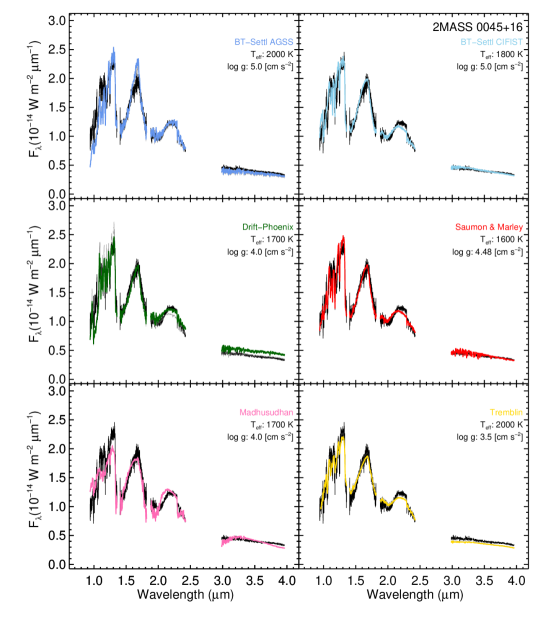
Figure 14: The combined spectrum of 2MASS 0045+16 (black) compared to the model spectra (colored). For ease of comparison, the near-IR best-fit models are shown in grey.

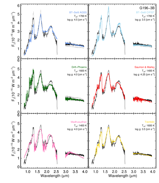
Figure 15: The combined spectrum of G196-3B (black) compared to the model spectra (colored). For ease of comparison, the near-IR best-fit models are shown in grey.

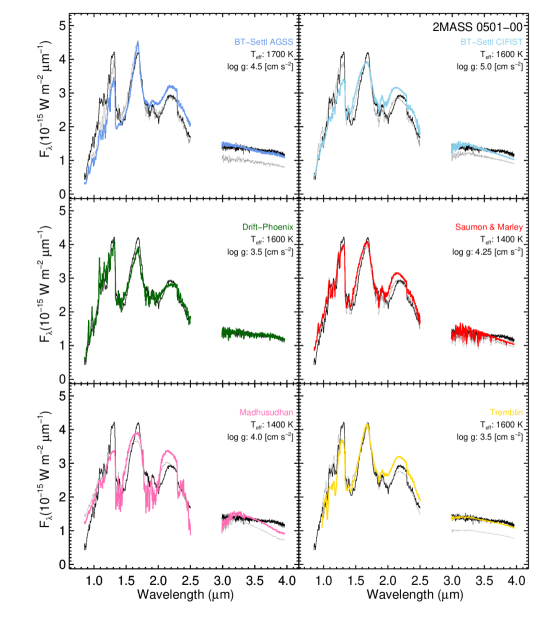
Figure 16: The combined spectrum of 2MASS 0501-00 (black) compared to the model spectra (colored). For ease of comparison, the near-IR best-fit models are shown in grey.

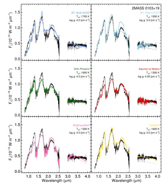
Figure 17: The combined spectrum of 2MASS 0103+19 (black) compared to the model spectra (colored). For ease of comparison, the near-IR best-fit models are shown in grey.

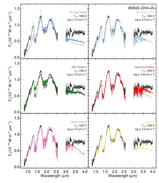
Figure 18: The combined spectrum of 2MASS 2244+20 (black) compared to the model spectra (colored). For ease of comparison, the near-IR best-fit models are shown in grey.

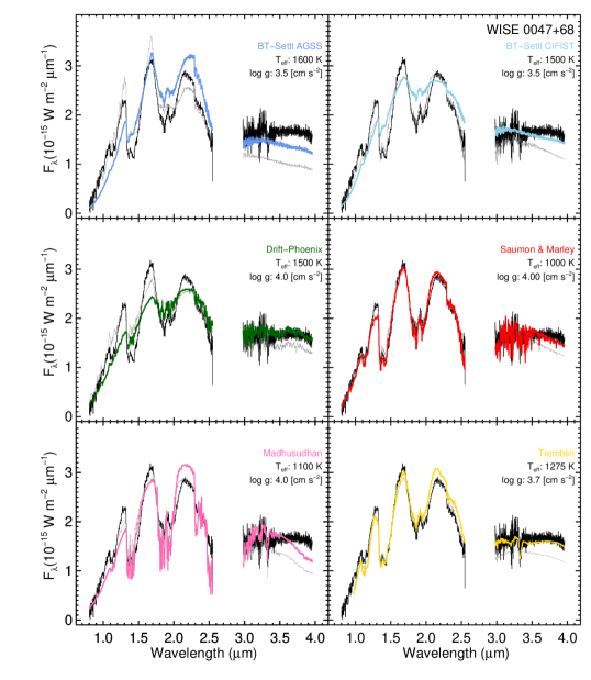
Figure 19: The combined spectrum of WISE 0047+68 (black) compared to the model spectra (colored). For ease of comparison, the near-IR best-fit models are shown in grey.

References

- Ackerman & Marley (2001) Ackerman, A. S. & Marley, M. S. 2001, ApJ, 556, 872. doi:10.1086/321540
- Akeson et al. (2013) Akeson, R. L., Chen, X., Ciardi, D., et al. 2013, PASP, 125, 989. doi:10.1086/672273
- Allard et al. (2012) Allard, F., Homeier, D., & Freytag, B. 2012, Philosophical Transactions of the Royal Society of London Series A, 370, 2765
- Allers et al. (2016) Allers, K. N., Gallimore, J. F., Liu, M. C., & Dupuy, T. J. 2016, ApJ, 819, 133
- Allers & Liu (2013) Allers, K. N., & Liu, M. C. 2013, ApJ, 772, 79
- Allers et al. (2010) Allers, K. N., Liu, M. C., Dupuy, T. J., & Cushing, M. C. 2010, ApJ, 715, 561
- Asplund et al. (2009) Asplund, M., Grevesse, N., Sauval, A. J., et al. 2009, ARA&A, 47, 481
- Barenfeld et al. (2013) Barenfeld, S. A., Bubar, E. J., Mamajek, E. E., et al. 2013, ApJ, 766, 6. doi:10.1088/0004-637X/766/1/6
- Barman et al. (2011) Barman, T. S., Macintosh, B., Konopacky, Q. M., & Marois, C. 2011, ApJ, 733, 65
- Best et al. (2020) Best, W., Dupuy, T. J., Liu, M. C., et al.,2020, The UltracoolSheet: Photometry, Astrometry, Spectroscopy, and Multiplicity for 3000+ Ultracool Dwarfs and Imaged Exoplanets, v1.01, Zenodo 10.5281/zenodo.4169085
- Burningham et al. (2021) Burningham, B., Faherty, J. K., Gonzales, E. C., et al. 2021, MNRAS, 506, 1944. doi:10.1093/mnras/stab1361
- Caffau et al. (2011) Caffau, E., Ludwig, H.-G., Steffen, M., et al. 2011, Sol. Phys., 268, 255
- Chauvin et al. (2005) Chauvin, G., Lagrange, A.-M., Dumas, C., et al. 2005, A&A, 438, L25
- Chilcote et al. (2017) Chilcote, J., Pueyo, L., De Rosa, R. J., et al. 2017, AJ, 153, 182
- Cohen et al. (2003) Cohen, M., Wheaton, W. A., & Megeath, S. T. 2003, AJ, 126, 1090
- Cruz et al. (2004) Cruz, K. L., Reid, I. N., Liebert, J., et al. 2004, VizieR Online Data Catalog, J/AJ/126/2421
- Cruz et al. (2009) Cruz, K. L., Kirkpatrick, J. D., & Burgasser, A. J. 2009, AJ, 137, 3345
- Cruz et al. (2018) Cruz, K. L., Núñez, A., Burgasser, A. J., et al. 2018, AJ, 155, 34
- Cutri et al. (2003) Cutri, R. M., Skrutskie, M. F., van Dyk, S., et al. 2003, “The IRSA 2MASS All-Sky Point Source Catalog, NASA/IPAC Infrared Science Archive.”
- Cushing et al. (2008) Cushing, M. C., Marley, M. S., Saumon, D., et al. 2008, ApJ, 678, 1372
- Cushing et al. (2004) Cushing, M. C., Vacca, W. D., & Rayner, J. T. 2004, PASP, 116, 362
- Dupuy & Kraus (2013) Dupuy, T. J., & Kraus, A. L. 2013, Science, 341, 1492
- Dupuy & Liu (2012) Dupuy, T. J. & Liu, M. C. 2012, ApJS, 201, 19. doi:10.1088/0067-0049/201/2/19
- Elias et al. (2006) Elias, J. H., Joyce, R. R., Liang, M., et al. 2006, Proc. SPIE, 6269, 62694C
- Faherty et al. (2012) Faherty, J. K., Burgasser, A. J., Walter, F. M., et al. 2012, ApJ, 752, 56
- Faherty et al. (2013) Faherty, J. K., Rice, E. L., Cruz, K. L., Mamajek, E. E., & Núñez, A. 2013, AJ, 145, 2
- Faherty et al. (2016) Faherty, J. K., Riedel, A. R., Cruz, K. L., et al. 2016, ApJS, 225, 10
- Filippazzo et al. (2015) Filippazzo, J. C., Rice, E. L., Faherty, J., et al. 2015, ApJ, 810, 158
- Gagné et al. (2014) Gagné, J., Lafrenière, D., Doyon, R., et al. 2014, ApJ, 783, 121. doi:10.1088/0004-637X/783/2/121
- Gagné et al. (2015) Gagné, J., Faherty, J. K., Cruz, K. L., et al. 2015, ApJS, 219, 33
- Gagné et al. (2018) Gagné, J., Fontaine, G., Simon, A., & Faherty, J. K. 2018, ApJ, 861, L13
- Gizis et al. (2012) Gizis, J. E., Faherty, J. K., Liu, M. C., et al. 2012, AJ, 144, 94
- Gizis et al. (2015) Gizis, J. E., Allers, K. N., Liu, M. C., et al. 2015, ApJ, 799, 203
- Hodapp et al. (2003) Hodapp, K. W., Jensen, J. B., Irwin, E. M., et al. 2003, PASP, 115, 1388
- Johnston et al. (2019) Johnston, V. D., Cushing, M. C., & Noll, K. S. 2019, Research Notes of the American Astronomical Society, 3, 52
- Kellogg et al. (2016) Kellogg, K., Metchev, S., Gagné, J., & Faherty, J. 2016, ApJ, 821, L15
- Kirkpatrick (2005) Kirkpatrick, J. D. 2005, ARA&A, 43, 195
- Kirkpatrick et al. (2006) Kirkpatrick, J. D., Barman, T. S., Burgasser, A. J., et al. 2006, ApJ, 639, 1120
- Kirkpatrick et al. (2008) Kirkpatrick, J. D., Cruz, K. L., Barman, T. S., et al. 2008, ApJ, 689, 1295
- Lagrange et al. (2009) Lagrange, A.-M., Gratadour, D., Chauvin, G., et al. 2009, A&A, 493, L21
- Landsman (1996) Landsman, W. B 1993 in Astronomical Data Analysis Software and Systems II, A.S.P. Conference Series, Vol. 52, ed. R. J. Hanisch, R. J. V. Brissenden, and Jeannette Barnes, p. 246.
- Leggett et al. (2007) Leggett, S. K., Saumon, D., Marley, M. S., et al. 2007, ApJ, 655, 1079
- Liu et al. (2013) Liu, M. C., Magnier, E. A., Deacon, N. R., et al. 2013, ApJ, 777, L20
- Liu et al. (2016) Liu, M. C., Dupuy, T. J., & Allers, K. N. 2016, ApJ, 833, 96
- Looper et al. (2008) Looper, D. L., Kirkpatrick, J. D., Cutri, R. M., et al. 2008, ApJ, 686, 528
- Lord (1992) Lord, S. D. 1992, NASA Technical Memorandum 103957,
- Luhman et al. (2009) Luhman, K. L., Mamajek, E. E., Allen, P. R., & Cruz, K. L. 2009, ApJ, 703, 399
- Madhusudhan et al. (2011) Madhusudhan, N., Burrows, A., & Currie, T. 2011, ApJ, 737, 34
- Males et al. (2014) Males, J. R., Close, L. M., Morzinski, K. M., et al. 2014, ApJ, 786, 32
- Mamajek et al. (2013) Mamajek, E. E., Bartlett, J. L., Seifahrt, A., et al. 2013, AJ, 146, 154
- Manjavacas et al. (2014) Manjavacas, E., Bonnefoy, M., Schlieder, J. E., et al. 2014, A&A, 564, A55. doi:10.1051/0004-6361/201323016
- Marley et al. (2010) Marley, M. S., Saumon, D., & Goldblatt, C. 2010, ApJ, 723, L117
- Marley et al. (2012) Marley, M. S., Saumon, D., Cushing, M., et al. 2012, ApJ, 754, 135
- Marois et al. (2008) Marois, C., Macintosh, B., Barman, T., et al. 2008, Science, 322, 1348
- Martin et al. (2017) Martin, E. C., Mace, G. N., McLean, I. S., et al. 2017, ApJ, 838, 73
- Metchev et al. (2015) Metchev, S. A., Heinze, A., Apai, D., et al. 2015, ApJ, 799, 154
- Miles et al. (2018) Miles, B. E., Skemer, A. J., Barman, T. S., et al. 2018, ApJ, 869, 18
- Noll et al. (2000) Noll, K. S., Geballe, T. R., Leggett, S. K., & Marley, M. S. 2000, ApJ, 541, L75
- Reach et al. (2005) Reach, W. T., Megeath, S. T., Cohen, M., et al. 2005, PASP, 117, 978. doi:10.1086/432670
- Reid et al. (2008) Reid, I. N., Cruz, K. L., Kirkpatrick, J. D., et al. 2008, AJ, 136, 1290
- Rice et al. (2010) Rice, E. L., Barman, T., Mclean, I. S., et al. 2010, ApJS, 186, 63
- Saumon et al. (2003) Saumon, D., Marley, M. S., Lodders, K., et al. 2003, Brown Dwarfs, 211, 345
- Saumon & Marley (2008) Saumon, D., & Marley, M. S. 2008, ApJ, 689, 1327
- Schneider et al. (2016) Schneider, A. C., Windsor, J., Cushing, M. C., Kirkpatrick, J. D., & Wright, E. L. 2016, ApJ, 822, L1
- Skemer et al. (2012) Skemer, A. J., Hinz, P. M., Esposito, S., et al. 2012, ApJ, 753, 14
- Skemer et al. (2014) Skemer, A. J., Marley, M. S., Hinz, P. M., et al. 2014, ApJ, 792, 17
- Stephens et al. (2009) Stephens, D. C., Leggett, S. K., Cushing, M. C., et al. 2009, ApJ, 702, 154
- Tokunaga & Vacca (2005) Tokunaga, A. T., & Vacca, W. D. 2005, PASP, 117, 421
- Tremblin et al. (2016) Tremblin, P., Amundsen, D. S., Chabrier, G., et al. 2016, ApJ, 817, L19
- Tremblin et al. (2017) Tremblin, P., Chabrier, G., Baraffe, I., et al. 2017, ApJ, 850, 46
- Vacca et al. (2003) Vacca, W. D., Cushing, M. C., & Rayner, J. T. 2003, PASP, 115, 389. doi:10.1086/346193
- Vos et al. (2018) Vos, J. M., Allers, K. N., Biller, B. A., et al. 2018, MNRAS, 474, 1041
- Witte et al. (2009) Witte, S., Helling, C., & Hauschildt, P. H. 2009, A&A, 506, 1367
- Zahnle & Marley (2014) Zahnle, K. J., & Marley, M. S. 2014, ApJ, 797, 41
- Zapatero Osorio et al. (2010) Zapatero Osorio, M. R., Rebolo, R., Bihain, G., et al. 2010, ApJ, 715, 1408
- Zuckerman et al. (2004) Zuckerman, B., Song, I., & Bessell, M. S. 2004, ApJ, 613, L65