Strain-induced superfluid transition for atoms on graphene

Abstract

Bosonic atoms deposited on atomically thin substrates represent a playground for exotic quantum many-body physics due to the highly-tunable, atomic-scale nature of the interaction potentials. The ability to engineer strong interparticle interactions can lead to the emergence of complex collective atomic states of matter, not possible in the context of dilute atomic gases confined in optical lattices. While it is known that the first layer of adsorbed helium on graphene is permanently locked into a solid phase, we show by a combination of quantum Monte Carlo and mean-field techniques, that simple isotropic graphene lattice expansion effectively unlocks a large variety of two-dimensional ordered commensurate, incommensurate, cluster atomic solid, and superfluid states for adsorbed atoms. It is especially significant that an atomically thin superfluid phase of matter emerges under experimentally feasible strain values, with potentially supersolid phases in close proximity on the phase diagram.

I Introduction

The quest to understand the behavior of strongly interacting electrons in quantum materials has led to a fruitful program of quantum simulation [1], where analogous quantum systems are constructed from well-understood and controllable constituents. Promising examples include the study of atoms confined in optical lattice potentials [2, 3, 4], electrons in two-dimensional (2D) materials – most notably graphene and its derivatives – [5, 6], Rydberg arrays [7], and superconducting quantum circuits [8]. Many of these approaches can realize lattice Hamiltonians on mesoscopic scales, or at low densities; however, generating strong interactions at the atomic scale remains a challenge. A promising route is the construction of synthetic matter where atoms are adsorbed onto a physical substrate solid with [9] or without chemical bonding [10, 11].

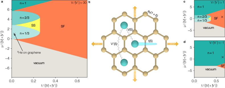
Figure 1: Strain-tuning the phase diagram. a The mean field phase diagram as a function of dimensionless chemical potential $\mu$ and hopping $t$ for hard-core bosons on the 2D triangular lattice with the ratio of nearest to next-nearest neighbor interactions $V/\absolutevalue{V^{\prime}}\simeq 30$ (the physically realized value as indicated by a $\times$ for ^4He on graphene [12] at fixed small $\mu$). Lobes with crystalline insulating phases appear at filling fractions $n=1/3,\,2/3,$ and $1$ as $\mu$ is increased for small $t$, and a superfluid phase (SF) is stable for larger $t$. A supersolid (SS) can exist between the lobes. Realizing non-solid order would require pushing the ^4He on graphene system to larger values of $t/(\absolutevalue{V}+\absolutevalue{V^{\prime}})$; however, the only experimental tuning parameter ($\mu$) is restricted to vertical movement in the phase diagram. b The effective Bose–Hubbard Hamiltonian describing ^4He atoms adsorbed on a suspended graphene membrane can be mechanically manipulated via isotropic biaxial strain that increases the C–C bond length by a fraction $\delta$. The resulting microscopic hopping $t$, nearest-neighbor $V$, and next-nearest neighbor $V^{\prime}$ interactions are found to be strong functions of $\delta$ (see Fig. 2), opening up the possibility of realizing superfluid order. c and d are modified mean field phase diagrams in the presence of strain for $V/\absolutevalue{V^{\prime}}\simeq 1$ and $V/\absolutevalue{V^{\prime}}\simeq-1$, respectively. The large reduction and change in sign of the nearest neighbor interaction $V$ as a function of $\delta$ has a drastic effect: ^4He on strained graphene (indicated by $\times$) may become superfluid, or admit a strongly correlated $n=1$ insulator.

Here we consider the latter case and study bosonic ^4He atoms adsorbed on graphene, where both atom-atom and atom-substrate interactions are driven by Van der Waals (VdW) dispersion forces. This is an ideal platform to study fundamental many-body phenomena such as the formation of solid, superfluid, and supersolid phases, as well as the quantum phase transitions between them. Adsorbed ^4He films have been a subject of considerable interest for over half a century and have drastically informed our understanding of criticality, including the role of the healing length [13] and the universal jump of the superfluid density at the Kosterlitz-Thouless transition [14]. For a flat crystalline substrate such as graphite, the presence of strong adsorption sites forming a triangular lattice (the dual lattice corresponding to graphite hexagon centers) produces a series of commensurate and incommensurate solid phases in the first layer of adsorbed ^4He observable by anomalies in the heat capacity [15, 16, 17, 18]. In the second and further adsorbed layers, the interacting bosonic ⁴He atoms can form a superfluid phase at a temperature $T_{\rm KT}$ below the bulk $T_{\lambda}$, which can be detected via third sound or a frequency shift of the adsorbed mass with torsional oscillator measurements [19, 20, 21]. Further details on the structure of the adsorbed phases and the resulting coverage–temperature phase diagram have been obtained by extensive numerical simulations exploiting various levels of approximation for the graphite–helium interaction [22, 23, 24, 25]. While it has ultimately been understood that bulk helium does not exhibit a supersolid phase – one that simultaneously breaks translational and gauge symmetries – the existence of supersolidity in models of hard-core bosons on the triangular lattice [26] makes adsorbed helium on graphite a potential platform for realizing exotic phases. Recent experimental results provide support for this scenario, arguing for intertwined superfluid and density wave order [27, 28, 29] for multiple layer helium films on pristine graphite surfaces. However, the first layer remains strongly bound to the surface and displays no evidence of superfluid behavior.

The propensity for insulating behavior of the helium atoms close to the substrate is a result of the relatively strong corrugation potential ($\sim$30\text{\,}\mathrm{K}\text{/}$$ from peak to valley), that localizes atoms through an exponential suppression of tunneling between triangular lattice adsorption sites. It is thus natural to consider replacing the graphite substrate with graphene, providing the same triangular lattice of adsorption sites, but with an attractive potential approximately 10% weaker. This has motivated a number of theoretical studies employing ab initio quantum Monte Carlo simulations [30, 31, 32, 33, 34, 35, 36]; however, the first layer appears to remain stubbornly insulating, providing little motivation for expanded experimental searches.

In this manuscript, we propose that quantum delocalized atomically thin superfluid phases of ^4He can be realized in this system through the application of even moderate (5–15%) biaxial (isotropic) strain to the graphene membrane. This is possible due to the fact that graphene – an atomically thin solid itself – can be mechanically strained along one [37, 38], or multiple axes [39, 40] to produce an isotropic increase in the carbon–carbon bond length. The extreme sensitivity of the system to strain arises due to the fact that the interaction between adsorbed ^4He atoms changes from a strong (hard-core) repulsion to a weak attractive VdW tail on the Angstrom scale [41], which is also the scale of the underlying graphene lattice potential. Thus small changes in the latter can lead to a very strong modification of atomic interactions. Consequently, graphene’s lattice potential can be viewed as an “effective 2D lattice” for the ^4He atoms with a period on the scale of atomic interactions. This setup is conceptually impossible to achieve for conventional dilute gases in optical lattices [2] which are soft-core, allowing multiple bosons per site, and may have only tunable kinetic energy. Instead, ^4He on graphene can realize an effective 2D hard-core Bose–Hubbard model with strain-dependent nearest ($V$) and next-nearest ($V^{\prime}$) neighbor interactions. Our intuitive picture is motivated by mean field calculations (Figure 1) and confirmed with large scale ab initio quantum Monte Carlo simulations of helium on strained graphene at low temperature that are finite size scaled to the thermodynamic limit. We conclude that this system is a highly tunable (via mechanical strain and pressure/chemical potential) platform for the experimental exploration and discovery of strictly two dimensional strongly interacting quantum phases of matter.

II Characterization and Strain-Tuning

^4He atoms of mass $m_{4}$ interacting with a biaxially strained suspended graphene membrane can be described by the microscopic many-body Hamiltonian:

$$H=-\frac{\hbar^{2}}{2m_{4}}\sum_{i=1}^{N}{\bf\it\nabla}_{i}^{2}+\sum_{i=1}^{N}\mathcal{V}_{\rm\graphene}({\bf\it r}_{i};\delta)+\sum_{i<j}\mathcal{V}({\bf\it r}_{i}-{\bf\it r}_{j})\,.$$ (1)

Here, $\mathcal{V}_{\graphene}$ is the adsorption potential experienced by an atom at spatial position ${\bf\it r}_{i}$ with strain captured by $\delta\equiv{a/a_{0}-1}$ quantifying the increase of the carbon–carbon distance $a$ with respect to its unstrained as-grown value $a_{0}\simeq$1.42\text{\,}\mathrm{\text{Å}}\text{/}$$. $\mathcal{V}_{\graphene}$ can be obtained by summing up all the individual VdW interactions between ^4He and the C atoms in the membrane, carefully considering the effects of strain on the electronic polarization of graphene itself [42] (see Methods section for more details). The interaction between ^4He atoms is captured by $\mathcal{V}$ which is known to high precision [41, 43]. Numerical simulations of Eq. (1) with $\delta=0$ at low temperature are consistent with the experimentally observed phase diagram for graphite. They demonstrate that as the pressure is increased from vacuum, there is a first order transition where a single layer is adsorbed, forming a commensurate incompressible solid phase dubbed C1/3 where ^4He atoms are localized around 1/3 of the strong binding sites of the $30\text{\,}\mathrm{\SIUnitSymbolDegree}\text{/}$ rotated triangular lattice with lattice constant $\sqrt{3}a_{0}$ corresponding to graphene hexagon centers. The C1/3 phase is stable over a range of chemical potentials [44, 34, 12] due to the strong repulsive interactions that induce an energy cost of $\mathcal{V}(\sqrt{3}a_{0})\approx$50\text{\,}\mathrm{K}\text{/}$$ per atom when nearest neighbor triangular sites are occupied increasing the filling beyond $n=1/3$. As the pressure of the proximate helium gas is further increased, eventually other commensurate and incommensurate phases can be realized due to energetic compensation by the chemical potential, including those with proliferated domain walls [34]. Beyond a triangular lattice filling fraction of $n\simeq 0.6$, it is energetically favorable to form a second layer (and beyond), but at all lower fillings, the width of the transverse wavefunction of the adsorbed atoms remains on the atomic scale (see supplemental Fig. 3).

This strongly 2D character was recently exploited to demonstrate that the first adsorbed layer of helium on unstrained graphene ($\delta=0$) is well characterized by an effective extended hard-core 2D Bose–Hubbard model [12, 11] with hopping $t$ and both nearest ($V$) and next-nearest neighbor ($V^{\prime}$) density–density interactions on the triangular lattice:

$${H}_{BH} =-t\sum_{\left\langle i,j\right\rangle}\left({b}_{i}^{\dagger}{b}_{j}^{\phantom{\dagger}}+{b}_{j}^{\dagger}{b}_{i}^{\phantom{\dagger}}\right)+V\sum_{\left\langle i,j\right\rangle}{n}_{i}{n}_{j}$$

$$\quad+V^{\prime}\sum_{\left\langle\left\langle i,j\right\rangle\right\rangle}{n}_{i}{n}_{j}-\mu\sum_{i}{n}_{i}\,.$$ (2)

Here $b^{\dagger}_{i}(b^{\phantom{\dagger}}_{i})$ creates(annihilates) a hard-core ^4He atom on site $i$ of the triangular lattice and $n_{i}=b^{\dagger}_{i}b^{\phantom{\dagger}}_{i}$ measures the number of atoms per site where $[b^{\phantom{\dagger}}_{i},b^{\dagger}_{j}]=\delta_{ij}$. $\expectationvalue{i,j}$ and $\expectationvalue{\expectationvalue{i,j}}$ indicate nearest and next-nearest neighbors respectively.

For ^4He on unstrained graphene ($\delta=0$) it is known from many-body as well as first principle ab initio methods [12] that $V$ is strongly repulsive, originating from the overlap of localized wavefunctions on the scale of the lattice spacing, while $V^{\prime}$ is much weaker and attractive, due to the VdW tail with the ratio $V/\absolutevalue{V^{\prime}}\simeq 30$.

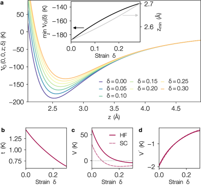
Figure 2: Strain-dependent adsorption and model parameters. a The microscopic helium–graphene adsorption potential $\mathcal{V}_{\graphene}$ that appears in Eq. (1) as a function of the height of an atom situated directly above a strong graphene adsorption site for different values of strain $\delta$. The inset quantifies how strain leads to a softening of the potential by reducing the binding energy per atom (left axis), as well as moving the location of the minimum, $z_{\rm min}$ (right axis) further from the membrane. Panels $\textbf{b}-\textbf{d}$ demonstrate the effects of biaxial strain on the effective 2D Bose–Hubbard model parameters $t$, $V$, and $V^{\prime}$ as computed via Hartree–Fock (HF) using the same method as described in Ref. [12]. Dashed lines correspond to the semi-classical (SC) predictions for the interaction parameters computed directly from the inter-atomic potential $\mathcal{V}$ evaluated at the expanded nearest and next-nearest neighbor distances assuming $\delta$-function wavefunctions. Panel c highlights the fact that at large strain, the nearest neighbor interaction $V$ can vanish, before changing signs and becoming attractive, which can lead to a drastic modification of the unstrained phase diagram.

The phase diagram of Eq. (2) can be directly computed at the mean field level [45] (see Methods), and it exhibits insulating phases at commensurate filling fractions $n=1/3,\,2/3,\,1$, as well as a superfluid and supersolid phase as a function of the dimensionless chemical potential $\mu$ and hopping $t$ as shown in Fig. 1a. The physical system of ^4He on graphene at fixed small $\mu$ is indicated by a cross ($\times$). By tuning the chemical potential (through the pressure of the proximate ^4He gas) an experiment could in principle observe the first order adsorption transition to a $n=1/3$ solid in the first layer. However, as the carbon atoms are moved further apart via strain, we expect that both $V$ and $V^{\prime}$ should be changed (Fig. 1b) leading to qualitative changes in the mean field phase diagram (as shown in Figure 1c and d). This culminates in access to both a superfluid and strongly correlated fully filled insulating phase as $V/V^{\prime}$ is reduced through zero.

To validate this simple picture and understand how the strain dependence of these effective parameters is generated in the physical helium on graphene system, we can analyze the adsorption potential $\mathcal{V}_{\graphene}$ and resulting effective parameters of the 2D Bose-Hubbard model for different values of $\delta$ as shown in Figure 2.

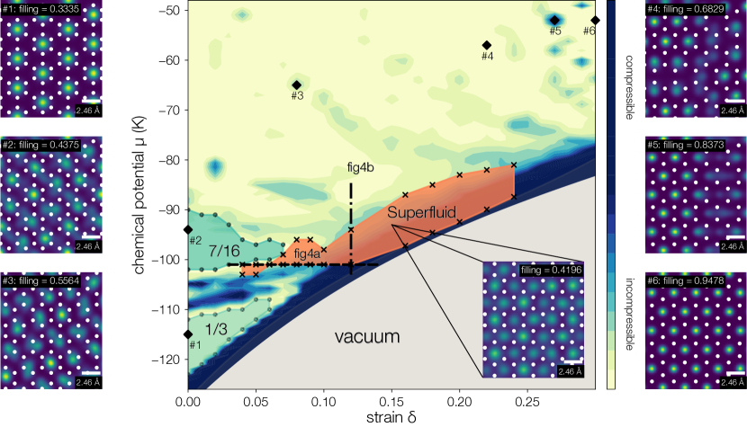
Figure 3: Superfluid phase diagram for helium adsorbed on strained graphene. Quantum Monte Carlo adsorbed particle configurations (halos #1–#6) and phase diagram (central panel) as a function of chemical potential $\mu$ and isotropic strain $\delta=a/a_{0}-1$ (enhancement of the carbon-carbon distance). The colored background of the main panel shows the compressibility of the adsorbed layer, with darker colors being more compressible. At small values of strain, large colored regions indicate commensurate solid phases with $n=1/3$ and $7/16$ of adsorption sites filled. As strain is increased, a superfluid phase (SF, orange) emerges with a critical temperature above $T=$0.5\text{\,}\mathrm{K}\text{/}$$ in thermodynamic limit, with a boundary indicated by $\times$ symbols. The behavior of the superfluid and particle density along the indicated horizontal and vertical cuts is shown in Figure 4. Sub-panels (halos #1–#6) show the average density of adsorbed helium at different regions of the phase diagram (indicated by $\blacklozenge$), detailing the particle configurations in both commensurate and incommensurate phases for $N_{\graphene}=48$ adsorption sites at $T=$1.0\text{\,}\mathrm{K}\text{/}$$. The filling fraction is indicated in each halo along with a scale bar highlighting the increase in the C-C separation, and the colorscale is set such that $\int\differential{x}\differential{y}\rho(x,y)=N$. At large strain, the unit filling phase predicted by mean field theory is observed in halo #6. It is important to note the adsorbed density in the superfluid phase (bottom right of central panel) is qualitatively different, exhibiting the delocalization of atoms between all adsorption sites.

In panel a, we demonstrate that for a single ^4He atom at position $z$ directly above the center of a graphene hexagon, as strain is increased, the adsorption potential becomes less attractive, with a minimum that softens by 30% from $-188\text{\,}\mathrm{K}\text{/}$ for $\delta=0$ to $-134\text{\,}\mathrm{K}\text{/}$ for $\delta=0.3$ corresponding to extreme strain as quantified in the inset. The location of the adsorbed 2D layer at this minimum, $z_{\rm min}$, is also pushed further from the sheet by 7%, from $2.5\text{\,}\mathrm{\text{Å}}\text{/}$ to $2.7\text{\,}\mathrm{\text{Å}}\text{/}$ yielding a concomitant reduction in the effect of the corrugation potential. This means, in essence, that the increase of $z_{\rm min}$ is correlated with the decrease of the effective barrier height related to the in-plane potential (calculated at $z_{\rm min}$), in turn, for example, causing an increase of atomic delocalization as a function of strain. These changes in the microscopic adsorption potential are reflected in the effective parameters of the Bose–Hubbard model as computed via Hartree–Fock calculations with the results shown in Figure 2b-d (see Methods section for details). They are calculated from the average interaction energy at the nearest and next-nearest neighbor level determined from the self-consistent adsorbed wavefunctions and compared with the strain dependence of the semi-classical (SC) predictions $V_{\rm SC}\equiv\mathcal{V}(\sqrt{3}(1+\delta)a_{0})$ and $V^{\prime}_{\rm SC}\equiv\mathcal{V}(3(1+\delta)a_{0})$ computed directly from the ^4He –^4He interaction potential. Here, SC refers to the use of point-particle wavefunctions with the full quantum potential $\mathcal{V}$. As can be seen in Figure 2b, the nearest neighbor interaction experiences a drastic reduction as $\delta$ is increased, with strong wavefunction renormalization effects, and vanishes near 19% strain, before becoming attractive for larger strains. As $V^{\prime}$ is controlled by the tail of the long-distance VdW interactions, and wavefunction effects have already been built into $\mathcal{V}$ at this scale, there is nearly perfect agreement between the semi-classical and the Hartree–Fock calculation.

III Superfluid Phase Diagram

The drastic decrease of $V$ in the effective Bose–Hubbard description due to strain engineering provides a route to increase the dimensionless hopping parameter $t/\quantity(\absolutevalue{V(\delta)}+\absolutevalue{V^{\prime}(\delta)})$ that controls the transition to the superfluid phase as detailed by the movement of the cross in Fig. 1. However, a number of questions remain regarding whether or not this is a realistic scenario for helium on graphene, as the extended Bose–Hubbard model describes only its 2D low energy sector, with the microscopic system allowing for a plethora of phases not present in the lattice model [25]. To validate these predictions, and generate a physical phase diagram, we have performed ab initio quantum Monte Carlo simulations of the full microscopic Hamiltonian in Eq. (1) for temperatures below $T_{\lambda}\simeq$2.17\text{\,}\mathrm{K}\text{/}$$, and over a wide range of chemical potentials and isotropic biaxial strains, up to 30%. The details of our simulations, based on the Feynman path integral formalism, are included in the Methods section, along with a description of how finite size graphene simulations for cells with dimension $L_{x}\times L_{y}$ were combined to extrapolate to the thermodynamic limit.

The combination of these simulations constitutes the most important result of this work, presented as a chemical potential $\mu$ – strain $\delta$ phase diagram in Figure 3. Here, the main panel shows the strain dependence of the first order phase transition from vacuum to a single adsorbed layer (see Supplementary Figure 4 for more details). It is pushed to larger chemical potentials as $\delta$ is increased, consistent with the softening of the adsorption potential highlighted in Figure 2. At low strain ($<5\%$), as the chemical potential is increased, we find commensurate phases with filling fractions $n=1/3$ and $n=7/16$ that have been previously observed in simulations of unstrained graphene [34] as well as experiments on graphite [18]. We note that the $n=7/16$ solid is not realized in the discrete lattice model, and is only energetically favorable in the presence of a continuous adsorption potential. As strain is further increased, the strong nearest-neighbor repulsion is reduced as the triangular lattice adsorption sites are moved further apart and the adsorbed layer moves further away from the membrane. Above 5% strain, there is a small range of fine-tuned chemical potentials near $\mu/k_{\rm B}=$-101\text{\,}\mathrm{K}\text{/}$$ where there is a transition from either a low density compressible liquid or vacuum to a superfluid. Here, superfluidity is quantified within the two-fluid picture where the total adsorbed density of atoms is broken into a normal and superfluid part with $\rho=\rho_{n}+\rho_{s}$ where $\rho=\expectationvalue{N}/(L_{x}L_{y})$ with $N$ the average number of adsorbed ^4He atoms. While this sliver persists in the thermodynamic limit, the superfluid density develops an aspect ratio dependence suggesting this region could be non-universal. For larger values with $\delta>0.1$, the extended superfluid region is more robust, extending up to 25% strain and over a range of chemical potentials. Within the superfluid phase, there is some evidence of competing solid order, but further work remains to be done to confirm the existence of a supersolid phase induced by the strained graphene lattice potential.

Surrounding the phase diagram are six halo figures showing the average density of particles superimposed on the strained graphene lattice, with the scale-bar representing the nearest neighbor distance for unstrained graphene $\sqrt{3}a_{0}\simeq$2.46\text{\,}\mathrm{\text{Å}}\text{/}$$. For $\delta=0$, commensurate phases with $n=1/3$ and $n=7/16$ are shown, while at larger strain and higher filling, phases with domain walls (e.g. #4 with $n\simeq 0.68$) are observed. For the strongest values of strain, the interaction between adsorbed ^4He atoms is dominated by the attractive long-range VdW tail, and a phase with unit filling is clearly observed as predicted by mean field theory (see Figure 1). Supplemental Figure 1 depicts the mean field phase diagram in the same physical units considered here. While there are quantitative modifications of boundaries, its major features are recovered with the exception of the $n=2/3$ insulator which is not energetically favorable in the presence of a continuum lattice potential.

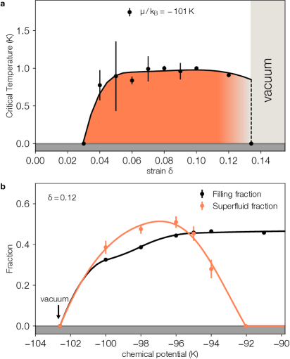
Figure 4: Details of the superfluid phase. a A horizontal cut at fixed chemical potential $\mu/k_{\rm B}=$-101\text{\,}\mathrm{K}\text{/}$$ indicated as a dashed line in Figure 3 shows the finite temperature onset of the superfluid phase as a function of strain. A non-vanishing superfluid fraction is measured up to the transition to the vacuum beyond $\delta=0.13$. b The particle filing fraction $n$ and superfluid fraction $\rho_{s}/\rho$ of the adsorbed atoms as a function of chemical potential $\mu$ at a fixed value of strain $(\delta=0.12)$ and temperature $T=$0.6\text{\,}\mathrm{K}\text{/}$$ (vertical dot-dashed line in Figure 3). In both panels, the error bars are computed as a combination of stochastic uncertainties from the Monte Carlo simulations and errors obtained from extrapolating to the thermodynamic limit. The smooth lines represent a guide to the eye.

More details on the superfluid phase can be obtained by taking horizontal and vertical cuts through Fig. 3 as shown in Figure 4. For fixed $\mu/k_{\rm B}=$-101\text{\,}\mathrm{K}\text{/}$$, the finite temperature strain phase diagram (panel a) shows the onset of a finite superfluid fraction near $\delta=0.03$ and the transition to vacuum for $\delta>0.13$. The critical temperature for the onset of superfluidity remains relatively constant near $T\approx$1\text{\,}\mathrm{K}\text{/}$$ over the entire phase. At a larger value of strain, $\delta=0.12$, Figure 4b tracks both the triangular lattice filling fraction $n$ and the superfluid fraction $\rho_{s}/\rho$ as a function of chemical potential, with the maximal signal occurring for a filling fraction $n\simeq 0.4$.

IV Discussion and Prospects for Measurement

Having analyzed the many-body phase diagram and identified a superfluid phase, it is natural to ask if this setup could be realized in a real experiment. Graphene is generally expected to withstand uniaxial mechanical strain of around 20% or more [46, 38], and several percent strain has already been realized [47, 37, 48]. On a fundamental level, it is important that strain can lead to substantial qualitative changes in electronic properties, which can be calculated with great theoretical precision, and consequently affect measurable physical characteristics [38, 49]. In principle, extreme uniaxial strain ($\sim 25\%$) can also lead to quantum phase transitions in the electronic structure of graphene itself. For example, a merger of Dirac cones can occur via a topological Lifshitz transition at a critical strain value [50], leading to the creation of an insulating state. The concept of “strain engineering,” i.e. manipulation of properties as a function of strain, is applicable to other classes of 2D materials as well, such as members of the dichalcogenide family (MoSe₂, MoS₂, WSe₂, WS₂) [38, 49, 51].

The combination of a strain-engineered 2D substrate with a proximate quantum gas opens up a new class of phenomena based on 2D material band structure modification. For graphene, isotropic biaxial strain – as considered here – is the “simplest” theoretical form of strain, and has been analyzed theoretically and realized experimentally [38, 40, 52, 39, 51]. As strain is applied equally along the armchair and zig-zag directions, the carbon–carbon lattice spacing changes isotropically (as captured by $\delta$). In this case, the graphene electronic dispersion remains isotropic (and electronically stable at any strain value the material can support), but the van der Waals forces that adatoms experience on top of graphene are substantially modified. As we have shown, the modification of interactions between bosonic adatoms can lead new low-dimensional quantum phases and quantum transitions between them. The competition between superfluid and correlated solid orders throughout the phase diagram opens up the possibility of realizing an adsorbed supersolid phase induced by the graphene adsorption potential with broken gauge and lattice symmetries. Our simulations on finite size graphene membranes host a large number of commensurate and incommensurate solid phases proximate to the identified superfluid, but the realization of a thermodynamically stable supersolid phase in the small region of phase space predicted by the mean field theory remains numerically elusive at this time.

In the laboratory, by combining well-known techniques to realize suspended graphene [53] with state-of-the art protocols that can simultaneously measure positional and superfluid responses of atoms adsorbed on flat surfaces [54, 55, 29], the phase diagram in Fig. 3 could be experimentally explored. Of course, it should be noted that such experiments are usually not performed under the “ideal” theoretical conditions assumed in our numerical modeling and could involve bending, proximity effects, strain asymmetry, etc. However, due to the ultra-rapid pace of technological developments in the field of 2D materials it is reasonable that such experiments are feasible in the near future.

V Methods

V.1 Mean Field Theory

Starting from the effective low-energy Bose–Hubbard Hamiltonian in Eq. (2), the interaction terms can be decoupled for each lattice site $i$ within the standard mean field approach, leading to:

$${H}_{MF,i} =-6t\quantity[\psi\quantity({b}^{\phantom{\dagger}}_{i}+{b}_{i}^{\dagger})-\psi^{2}]$$

$$\quad+6\left(V+V^{\prime}\right)\left(\rho{n}_{i}-\frac{\rho^{2}}{2}\right)-\mu{n}_{i},$$ (3)

where we have introduced the condensate density ${\displaystyle\langle b^{\phantom{\dagger}}_{i}\rangle=\langle b_{i}^{\dagger}\rangle=\psi}$ and the localized density ${\displaystyle\langle n_{i}\rangle=\rho.}$ For an insulating state, $\psi=0$. Diagonalizing in the basis of localized Wannier states [12] gives the ground state energy (per lattice site)

$$E =6t\psi^{2}+3\left(V+V^{\prime}\right)\rho\left(1-\rho\right)-\frac{\mu}{2}$$

$$\quad-\sqrt{\left(\frac{\mu-6\left(V+V^{\prime}\right)\rho}{2}\right)^{2}+\left(6t\psi\right)^{2}}\,.$$ (4)

The self-consistent eigenstates can be found by solving ${\displaystyle\partial_{\rho}E=\partial_{\psi}E=0}$, yielding the particle and condensate densities as:

$$\rho =\frac{6t+\mu}{12t+6\left(V+V^{\prime}\right)}$$ (5)

$$\psi =\frac{\sqrt{\left(6t+\mu\right)\left(6t+6\left(V+V^{\prime}\right)-\mu\right)}}{12t+6\left(V+V^{\prime}\right)}\,.$$ (6)

Energies of the solid phases are obtained as expectation values of the full Bose–Hubbard Hamiltonian Eq. (2) in states with corresponding fillings $(1/3,2/3,1)$ on the triangular unit cell. Normalizing energies and chemical potential by the scale $\absolutevalue{V}+\absolutevalue{V^{\prime}}$, we may write the dimensionless per-site energies of the solid and superfluid (SF) phases as:

$$\tilde{E}_{1/3} =\frac{-\tilde{\mu}}{3}-\frac{1}{\alpha+1}$$

$$\tilde{E}_{2/3} =\frac{-2\tilde{\mu}}{3}+\frac{\text{sgn}(V)\alpha-2}{\alpha+1}$$

$$\tilde{E}_{1} =-\tilde{\mu}+3\frac{\text{sgn}(V)\alpha-1}{\alpha+1}$$

$$\tilde{E}_{SF} =-\frac{\left(6\tilde{t}+\tilde{\mu}\right)^{2}(\alpha+1)}{24\tilde{t}(\alpha+1)+12\ \quantity[\text{sgn}(V)\alpha-1]}$$

where we have introduced the notation $\tilde{c}\equiv c/\quantity(\absolutevalue{V}+\absolutevalue{V^{\prime}})$, and defined $\alpha\equiv\absolutevalue{V/V^{\prime}}$, with $\text{sgn}(\dots)$ the signum function.

To capture a possible supersolid phase (defined as one having simultaneously broken translational and gauge symmetries), we allow for more degrees of freedom in the mean field decomposition. Considering the triangular unit cell with sites ${\displaystyle A,\,B,\,C}$, we assume

$$\psi_{A}\neq\psi_{B}=\psi_{C}$$

$$\rho_{A}\neq\rho_{B}=\rho_{C}.$$

Decoupling the mean field Hamiltonian in Eq. (3) for each unit cell yields

$$H_{MF,\triangle}=H_{t}+H_{V}+H_{V^{\prime}}+H_{\mu},$$

where

$$H_{t} =-3t\left[2\psi_{B}\left(b_{A}+b_{A}^{\dagger}\right)+\left(\psi_{A}+\psi_{B}\right)\left(b_{B}+b_{B}^{\dagger}\right.\right.$$

$$\quad\left.+b_{C}+b_{C}^{\dagger}\right)-4\psi_{A}\psi_{B}-2\psi_{B}^{2}\Bigl{]}$$

$$H_{V} =3V\left[2\rho_{B}n_{A}+\left(\rho_{A}+\rho_{B}\right)\left(n_{B}+n_{C}\right)-2\rho_{A}\rho_{B}-\rho_{B}^{2}\right]$$

$$H_{V^{\prime}} =3V^{\prime}\left[2\rho_{A}n_{A}+2\rho_{B}\left(n_{B}+n_{C}\right)-\rho_{A}^{2}-2\rho_{B}^{2}\right]$$

$$H_{\mu} =-\mu\left(n_{A}+n_{B}+n_{C}\right).$$

The energy $E_{SS}$ of the resulting state can be found by numerical solution of

$$\partial_{\psi_{A}}E=\partial_{\psi_{B}}E=\partial_{\rho_{A}}E=\partial_{\rho_{B}}E=0$$

at each point in ${\displaystyle\tilde{\mu}-\tilde{t}}$ phase space.

The values of $V$ and $V^{\prime}$ to be used can be determined by Hartree–Fock calculations (see next section) as a function of biaxial strain $\delta$. Three distinct physical regimes arise in terms of their relative magnitudes as discussed in the main text:

$$\begin{array}[]{cll}|V|\gg|V^{\prime}|&,\;V>0&\text{unstrained}\\ |V|\simeq|V^{\prime}|&,\;V>0&\text{moderate strain}\\ |V|\simeq|V^{\prime}|&,\;V<0&\text{large strain}.\end{array}$$

Thus, by fixing the ratio $\absolutevalue{V/V^{\prime}}$, mean field phase diagrams can be generated, as shown in Fig. 1. To obtain a realistic phase diagram for the ^4He-on-graphene system over a range of physical parameters, the full Hartree–Fock results for $t(\delta)$, $V(\delta)$, and $V^{\prime}(\delta)$ can be used directly, which leads to supplementary Figure S1.

V.2 Hartree–Fock

Since multi-particle quantum Monte Carlo simulations are time-consuming, we employed a computationally cheaper method, based on the Hartree–Fock (HF) approximation, to compute $V$ and $V^{\prime}$ in Eq. (2) to be used in the strain-tuned mean field phase diagram. The HF ansatz for the wavefunction $\Psi$ for $N$ bosons is:

$$\Psi(\mathbf{r}_{1},\mathbf{r}_{2},\ldots,\mathbf{r}_{N})=\sum_{j(q)}\,\prod_{q=1}^{N}\phi_{j(q)}(\mathbf{r}_{q}),$$ (7)

where $\mathbf{r}_{q}$ are the 3D coordinates of particle $q$, $j(q)$ is a label of the site where particle $q$ is found, and the one-particle quasi-wavefunctions (in what follows we will drop “quasi”) satisfy the orthonormality conditions

$$\langle\phi_{i}|\phi_{j}\rangle\equiv\int d^{2}\mathbf{r}\,\phi^{\dagger}_{i}(\mathbf{r})\phi_{j}(\mathbf{r})=\delta_{i,j}\,,$$ (8)

and the $\dagger$ stands for Hermitian conjugation. Employing an approximation $\phi_{i}(\mathbf{r})\approx\chi(z)\psi_{i}(\!\mathbf{{{\mathcalligra{r}}}})$, where $\!\mathbf{{{\mathcalligra{r}}}}$ is the 2D coordinate in the plane parallel to the graphene sheet and $z$ is the perpendicular coordinate, the 2D-reduced wavefunction can be shown to satisfy HF equations:

$$-\frac{\hbar^{2}}{2m}\nabla^{2}_{\!\mathbf{{{\mathcalligra{r}}}}}\psi_{i}(\!\mathbf{{{\mathcalligra{r}}}})+{\mathcal{V}}_{\graphene}(\!\mathbf{{{\mathcalligra{r}}}})\psi_{i}(\!\mathbf{{{\mathcalligra{r}}}})\\ +\sum_{i\neq j}\int\differential{\!\mathbf{{{\mathcalligra{r}}}}^{\prime}}\,\psi_{j}^{\ast}(\!\mathbf{{{\mathcalligra{r}}}}^{\prime})\mathcal{V}(\!\mathbf{{{\mathcalligra{r}}}}-\!\mathbf{{{\mathcalligra{r}}}}^{\prime})\\ \times\left[\psi_{j}(\!\mathbf{{{\mathcalligra{r}}}}^{\prime})\psi_{i}(\!\mathbf{{{\mathcalligra{r}}}})+\psi_{i}(\!\mathbf{{{\mathcalligra{r}}}}^{\prime})\psi_{j}(\!\mathbf{{{\mathcalligra{r}}}})\right]=\sum_{j}E_{ij}\psi_{j}(\!\mathbf{{{\mathcalligra{r}}}})\,,$$ (9)

where the Lagrange multipliers $E_{ij}$ are determined by the 2D form of the orthonormality conditions (8). Details of these approximations, as well as of the solution method of (9), were outlined in [12]. In (9), ${\mathcal{V}}_{\rm\graphene}(\!\mathbf{{{\mathcalligra{r}}}})$ is computed as:

$$\mathcal{V}_{\graphene}(\!\mathbf{{{\mathcalligra{r}}}})\equiv\expectationvalue{\frac{\int\differential{z}\mathcal{V}_{\graphene}(\!\mathbf{{{\mathcalligra{r}}}},z)\rho(\!\mathbf{{{\mathcalligra{r}}}},z)}{\int\differential{z}\rho(\!\mathbf{{{\mathcalligra{r}}}},z)}}$$ (10)

where $\rho(\!\mathbf{{{\mathcalligra{r}}}},z)$ is the probability density obtained with one-particle (and hence relatively fast) QMC simulations and the angle brackets stand for the ensemble average. Furthermore, $\mathcal{V}(\!\mathbf{{{\mathcalligra{r}}}})$ is the 2D-reduction (as explained in [12]) of the interaction potential $\mathcal{V}(\!\mathbf{{{\mathcalligra{r}}}},z)$ between two helium atoms. In a slight deviation from [12], here for the computation of this reduced 2D potential, we used the one-dimensional probability density $\rho(z)\equiv\int\differential{\!\mathbf{{{\mathcalligra{r}}}}}\rho(\!\mathbf{{{\mathcalligra{r}}}},z)$, with the $\rho(\!\mathbf{{{\mathcalligra{r}}}},z)$ as defined above. Then, parameter $V$ in (2) is computed as:

$$V=\int\int\differential{\!\mathbf{{{\mathcalligra{r}}}}}\,\differential{\!\mathbf{{{\mathcalligra{r}}}}^{\prime}}\,|\psi_{i}(\!\mathbf{{{\mathcalligra{r}}}})|^{2}\mathcal{V}(\!\mathbf{{{\mathcalligra{r}}}}-\!\mathbf{{{\mathcalligra{r}}}}^{\prime})|\psi_{j}(\!\mathbf{{{\mathcalligra{r}}}}^{\prime})|^{2},$$ (11)

where $i$ and $j$ are the indices of the two nearest-neighbor graphene cells. Parameter $V^{\prime}$ is defined similarly, but for the next-nearest neighbors. Finally, parameter $t$ is computed as described in [12], using one-particle Wannier functions for a single helium atom over the graphene sheet.

V.3 Quantum Monte Carlo

The strained graphene plus ^4He system described by the Hamiltonian in Eq. (1) was simulated using a stochastically exact quantum Monte Carlo (QMC) algorithm exploiting path integrals [56, 57, 12]. Finite temperature expectation values of observables $\mathcal{O}$ were sampled via

$$\expectationvalue{{\mathcal{O}}}=\frac{1}{\mathcal{Z}}\Tr(\mathcal{O}\ \mathrm{e}^{-\beta{{H}}})$$ (12)

where $\beta=1/k_{\rm{B}}T$ is the inverse temperature, $k_{\rm B}$ is the Boltzmann constant, and the partition function $\mathcal{Z}=\Tr\mathrm{e}^{-\beta{{H}}}$ can be written as a sum of discrete imaginary time paths (worldlines) over the set of all permutations $\mathcal{P}$ of the first quantized labels of the $N$ indistinguishable ⁴He atoms. Algorithmic details have been reported elsewhere (e.g. Refs. [58, 12, 59]) and access to the QMC software is described in the Code Availability Section.

V.3.1 Simulation Cell

The simulation cell is defined by a rectangular prism of dimensions $L_{x}\times L_{y}\times L_{z}$ where $L_{x}$ and $L_{y}$ are chosen such that the strained graphene sheet is compatible with periodic boundary conditions in the $x$ and $y$ directions. A membrane with $N_{\graphene}=2N_{x}N_{y}$ triangular lattice adsorption sites requires that $L_{x}=a_{0}(1+\delta)\sqrt{3}N_{x}$ for the zigzag direction and $L_{y}=3a_{0}(1+\delta)N_{y}$ for the armchair direction. Three of the box sizes corresponding to different numbers of adsorption sites used for finite size scaling our QMC results to the thermodynamic limit are shown in Fig. 5.

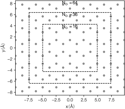
Figure 5: Finite size simulation cell. Three system sizes were used for finite size scaling where periodic boundary conditions restrict the box dimensions to be a multiple of lattice vectors in the $x$ and $y$ directions. The resulting box size is a function of strain $\delta$ and $N_{\graphene}$ refers to the number of triangular lattice adsorption sites in the simulation cell.

The strained graphene membrane is frozen in place at $z=0$ with lattice (${\bf\it a}$) and basis (${\bf\it b}$) vectors:

$${\bf\it a}_{1}(\delta) =\frac{a_{0}(1+\delta)}{2}\quantity(\sqrt{3},3), {\bf\it b}_{1}(\delta) =\frac{a_{0}(1+\delta)}{2}\quantity(\sqrt{3},1)$$ (13)

$${\bf\it a}_{2}(\delta) =\frac{a_{0}(1+\delta)}{2}\quantity(-\sqrt{3},3), {\bf\it b}_{2}(\delta) =a_{0}(1+\delta)\quantity(0,1)$$

where $a_{0}\simeq$1.42\text{\,}\mathrm{\text{Å}}\text{/}$$ is the bare carbon–carbon distance and $0\leq\delta\leq 1$ represents its increase under isotropic strain. Motion in the $z$ direction is restricted via a hard wall placed at $z=L_{z}=$10\text{\,}\mathrm{\text{Å}}\text{/}$$, chosen to reproduce bulk multi-layer adsorption phenomena [12].

The resulting empirical interaction potential $\mathcal{V}_{\graphene}$ between ^4He and the strained graphene is computed by assuming a superposition of 6–12 Lennard–Jones potentials between carbon and helium [60]:

$$\!\!\!\!\mathcal{V}_{\graphene}({\bf\it r}_{i})=\frac{8\pi\varepsilon(\delta)\sigma^{2}(\delta)}{3\sqrt{3}a_{0}^{2}(1+\delta)^{2}}\left\{\quantity[\frac{2}{5}\quantity(\frac{\sigma(\delta)}{z_{i}})^{10}\!\!\!\!-\quantity(\frac{\sigma(\delta)}{z_{i}})^{4}]\right.\\ +\sum_{{\bf\it g}\neq 0}\sum_{\ell=1}^{2}\mathrm{e}^{\imath{\bf\it g}(\delta)\cdot[\!\mathbf{{{\mathcalligra{r}}}}_{i}-{\bf\it b}_{\ell}(\delta)]}\left[\frac{1}{60}\quantity(\frac{g(\delta)\sigma(\delta)^{2}}{2z_{i}})^{5}K_{5}(g(\delta)z_{i})\right.\\ \left.\left.-\quantity(\frac{g(\delta)\sigma(\delta)^{2}}{2z_{i}})^{2}K_{2}(g(\delta)z_{i})\right]\right\}\,,$$ (14)

where $\sigma(\delta)$ and $\varepsilon(\delta)$ are strain-dependent Lennard–Jones parameters that have been computed via the method described in Ref. [42] with values and tabulated potentials (up to $\delta=0.3$) available online [61]. In Eq. (14), $\!\mathbf{{{\mathcalligra{r}}}}_{i}=(x_{i},y_{i})$ are the coordinates of a ⁴He atom in the $xy$-plane, and ${\bf\it g}(\delta)=n_{1}{\bf\it G}_{1}(\delta)+n_{2}{\bf\it G}_{2}(\delta)$ are the reciprocal lattice vectors with magnitude $g(\delta)\equiv\absolutevalue{{\bf\it g}(\delta)}$ where $n_{1},n_{2}\in\mathds{Z}$,

$${\bf\it G}_{1}(\delta) =\frac{2\pi}{3a_{0}(1+\delta)}\quantity(\sqrt{3},1)\,,$$

$${\bf\it G}_{2}(\delta) =\frac{2\pi}{3a_{0}(1+\delta)}\quantity(-\sqrt{3},1)$$ (15)

and $K_{n}$ are modified Bessel functions which decay as $\exp(-gz_{i})$ at large argument.

V.3.2 Observables

To map out the phase diagram reported in Fig. 3, we have computed a number of observables obtained via quantum Monte Carlo estimators. The total number of particles $N$ can fluctuate in the grand canonical ensemble at fixed temperature $T$ and chemical potential $\mu$ leading to an average value $\expectationvalue{N}$ and filling fraction:

$$n\equiv\frac{\expectationvalue{N}}{N_{\graphene}}$$ (16)

where $N_{\graphene}$ is set by the geometry of the simulation cell, and utilizing the fact that all atoms are adsorbed. The density of ^4He is given by:

$$\rho({\bf\it r})=\expectationvalue{\frac{1}{N}\sum_{i=1}^{N}\delta({\bf\it r}-{\bf\it r}_{i})}$$ (17)

where $\delta(\dots)$ is the Dirac delta-function. The planar density of ^4He adsorbed to the graphene can be computed by integrating over $z$: $\rho(x,y)=\int dz\rho({\bf\it r})$ and its resulting compressibility is given by the usual fluctuation measure:

$$\kappa=\frac{\expectationvalue{N^{2}}-\expectationvalue{N}^{2}}{k_{\rm B}TL_{x}L_{y}}\,.$$ (18)

Finally, the superfluid density $\rho_{s}$ is related to the response of the free energy to a boundary phase twist [62] which can be captured in QMC via the topological winding number ${\bf\it W}$ of particle worldlines around the simulation cell [63, 64, 65]:

$$\rho_{s}=\frac{m_{4}^{2}}{2\hbar^{2}\beta L_{x}L_{y}}\quantity(L_{x}^{2}\expectationvalue{W_{x}^{2}}+L_{y}^{2}\expectationvalue{W_{y}}^{2})$$ (19)

where

$${W}_{x}=\frac{1}{L_{x}}\sum_{i=1}^{N}\int_{0}^{\hbar\beta}\differential{\tau}\quantity[\derivative{x_{i}(\tau)}{\tau}]\,.$$ (20)

with $m_{4}$ the mass of a ^4He atom and $x_{i}(\tau)$ is the $x$-coordinate of the imaginary time wordline corresponding to atom $i$.

V.3.3 Simulation Details and Finite Size Scaling

Quantum Monte Carlo calculations were performed using open source software [66] for $T=$0.5\text{\,}\mathrm{K}\text{/}2.0\text{\,}\mathrm{K}\text{/}$$ and chemical potentials $\mu/k_{\rm B}$ from $-129\text{\,}\mathrm{K}\text{/}-41\text{\,}\mathrm{K}\text{/}$ at four system sizes corresponding to $N_{\graphene}=16,36,64,144$ triangular lattice adsorption sites to obtain particle configurations at values of the isotropic strain $\delta=0$ (unstrained) to $\delta=0.3$ (strongly strained). The imaginary time step was fixed at $k_{\rm B}\tau=$0.003\,13\text{\,}\mathrm{K}^{-1}$$ such that any systematic effects due to Trotterization are smaller than statistical sampling errors.

By searching for stable plateaus in the filling fraction $n$ at different values of $\delta$ that correspond to vanishing compressibility, we identified commensurate insulating phases corresponding to fillings of $n=1/3,7/6$, and $1$. The vacuum phase boundary in Fig. 3 corresponds to the line denoting a non-zero expectation value $\expectationvalue{N}\geq 0$.

While particle configurations are reported at fixed system sizes, superfluid and particle densities were obtained via a finite size scaling procedure at each temperature to extrapolate to the thermodynamic limit for the cell sizes depicted in Fig. 5. Details are included in Supplemental Figure 2, where we have assumed the finite size scaling forms $n(N)=n|_{\infty}+O(1/N)$ and $\rho_{s}(N)=\rho_{s}|_{\infty}+O(1/\sqrt{N})$. The superfluid phase boundary in Fig. 3 was determined by performing this finite size scaling procedure at 65 $(\delta,\mu)$ points and identifying as superfluid any point where $\rho_{s}$ persists to the thermodynamic limit for temperatures greater than $T=$0.5\text{\,}\mathrm{K}\text{/}$$ (the base $T$ in our quantum Monte Carlo study).

Error bars on composite estimators (such as the compressibility) were estimated via jackknife sampling [67].

VI Data Availability

The raw quantum Monte Calro simulation data set is available at https://zenodo.org/record/7271852 [68] while the processed data can be found online https://github.com/DelMaestroGroup/papers-code-Superfluid4HeStrainGraphene [69].

.

VII Code Availability

The code and scripts used to process data and generate all figures in this paper are available online at https://github.com/DelMaestroGroup/papers-code-Superfluid4HeStrainGraphene [69]. The path integral quantum Monte Carlo software used to generate all raw data is available online at https://github.com/DelMaestroGroup/pimc [66].

VIII Acknowledgments

This work was supported by NASA grant number 80NSSC19M0143. Computational resources were provided by the NASA High-End Computing (HEC) Program through the NASA Advanced Supercomputing (NAS) Division at Ames Research Center.

See pages 1, of supplement See pages 0, of supplement

References

- Altman et al. [2021] E. Altman, K. R. Brown, G. Carleo, L. D. Carr, E. Demler, C. Chin, B. DeMarco, S. E. Economou, M. A. Eriksson, K.-M. C. Fu, M. Greiner, K. R. A. Hazzard, R. G. Hulet, A. J. Kollár, B. L. Lev, M. D. Lukin, R. Ma, X. Mi, S. Misra, C. Monroe, K. Murch, Z. Nazario, K.-K. Ni, A. C. Potter, P. Roushan, M. Saffman, M. Schleier-Smith, I. Siddiqi, R. Simmonds, M. Singh, I. B. Spielman, K. Temme, D. S. Weiss, J. Vučković, V. Vuletić, J. Ye, and M. Zwierlein, Quantum Simulators: Architectures and Opportunities, PRX Quantum 2, 017003 (2021).
- Bloch et al. [2008] I. Bloch, J. Dalibard, and W. Zwerger, Many-body physics with ultracold gases, Rev. Mod. Phys. 80, 885 (2008).
- Lewenstein et al. [2007] M. Lewenstein, A. Sanpera, V. Ahufinger, B. Damski, A. Sen(De), and U. Sen, Ultracold atomic gases in optical lattices: mimicking condensed matter physics and beyond, Adv. Phys. 56, 243 (2007).
- Zhang et al. [2018] D.-W. Zhang, Y.-Q. Zhu, Y. X. Zhao, H. Yan, and S.-L. Zhu, Topological quantum matter with cold atoms, Adv. Phys. 67, 253 (2018).
- Castro Neto et al. [2009] A. H. Castro Neto, F. Guinea, N. M. R. Peres, K. S. Novoselov, and A. K. Geim, The electronic properties of graphene, Rev. Mod. Phys. 81, 109 (2009).
- Geim and Grigorieva [2013] A. K. Geim and I. Grigorieva, Van der Waals heterostructures, Nature 499, 419 (2013).
- Semeghini et al. [2021] G. Semeghini, H. Levine, A. Keesling, S. Ebadi, T. T. Wang, D. Bluvstein, R. Verresen, H. Pichler, M. Kalinowski, R. Samajdar, A. Omran, S. Sachdev, A. Vishwanath, M. Greiner, V. Vuletić, and M. D. Lukin, Probing topological spin liquids on a programmable quantum simulator, Science 374, 1242 (2021).
- Ma et al. [2019] R. Ma, B. Saxberg, C. Owens, N. Leung, Y. Lu, J. Simon, and D. I. Schuster, A dissipatively stabilized Mott insulator of photons, Nature 566, 51 (2019).
- Ming et al. [2022] F. Ming, X. Wu, C. Chen, K. D. Wang, P. Mai, T. A. Maier, J. Strockoz, J. W. F. Venderbos, C. Gonzalez, J. Ortega, S. Johnston, and H. H. Weitering, Evidence for chiral superconductivity on a silicon surface (2022), arXiv:2210.06273 .
- Kreisel et al. [2021] A. Kreisel, T. Hyart, and B. Rosenow, Tunable topological states hosted by unconventional superconductors with adatoms, Phys. Rev. Research 3, 033049 (2021).
- Del Maestro et al. [2021] A. Del Maestro, C. Wexler, J. M. Vanegas, T. Lakoba, and V. N. Kotov, A perspective on Collective Properties of Atoms on 2D materials, Adv. Electron. Mater. 8, 2100607 (2021).
- Yu et al. [2021] J. Yu, E. Lauricella, M. Elsayed, K. Shepherd, N. S. Nichols, T. Lombardi, S. W. Kim, C. Wexler, J. M. Vanegas, T. Lakoba, V. N. Kotov, and A. Del Maestro, Two-dimensional Bose-Hubbard model for helium on graphene, Phys. Rev. B 103, 235414 (2021).
- Henkel et al. [1969] R. Henkel, E. Smith, and J. Reppy, Temperature Dependence of the Superfluid Healing Length, Phys. Rev. Lett. 23, 1276 (1969).
- Agnolet et al. [1989] G. Agnolet, D. F. McQueeney, and J. D. Reppy, Kosterlitz-Thouless transition in helium films, Phys. Rev. B 39, 8934 (1989).
- Bretz and Dash [1971] M. Bretz and J. Dash, Quasiclassical and Quantum Degenerate Helium Monolayers, Phys. Rev. Lett. 26, 963 (1971).
- Bretz et al. [1973] M. Bretz, J. G. Dash, D. C. Hickernell, E. O. McLean, and O. E. Vilches, Phases of He3 and He4 Monolayer Films Adsorbed on Basal-Plane Oriented Graphite, Phys. Rev. A 8, 1589 (1973).
- Zimmerli and Chan [1988] G. Zimmerli and M. H. W. Chan, Complete wetting of helium on graphite, Phys. Rev. B 38, 8760 (1988).
- Greywall and Busch [1991] D. S. Greywall and P. A. Busch, Heat capacity of fluid monolayers of 4He, Phys. Rev. Lett. 67, 3535 (1991).
- Zimmerli et al. [1992] G. Zimmerli, G. Mistura, and M. H. W. Chan, Third-sound study of a layered superfluid film, Phys. Rev. Lett. 68, 60 (1992).
- Crowell and Reppy [1996] P. A. Crowell and J. D. Reppy, Superfluidity and film structure in He4 adsorbed on graphite, Phys. Rev. B 53, 2701 (1996).
- Nyéki et al. [1998] J. Nyéki, R. Ray, B. Cowan, and J. Saunders, Superfluidity of Atomically Layered 4he Films, Phys. Rev. Lett. 81, 152 (1998).
- Whitlock et al. [1998] P. A. Whitlock, G. V. Chester, and B. Krishnamachari, Monte Carlo simulation of a helium film on graphite, Phys. Rev. B 58, 8704 (1998).
- Corboz et al. [2008] P. Corboz, M. Boninsegni, L. Pollet, and M. Troyer, Phase diagram of 4He adsorbed on graphite, Phys. Rev. B 78, 245414 (2008).
- Pierce and Manousakis [2000] M. E. Pierce and E. Manousakis, Role of substrate corrugation in helium monolayer solidification, Phys. Rev. B 62, 5228 (2000).
- Ahn et al. [2016] J. Ahn, H. Lee, and Y. Kwon, Prediction of stable C7/12 and metastable C4/7 commensurate solid phases for 4He on graphite, Phys. Rev. B 93, 064511 (2016).
- Wessel and Troyer [2005] S. Wessel and M. Troyer, Supersolid Hard-Core Bosons on the Triangular Lattice, Phys. Rev. Lett. 95, 127205 (2005).
- Nakamura et al. [2016] S. Nakamura, K. Matsui, T. Matsui, and H. Fukuyama, Possible quantum liquid crystal phases of helium monolayers, Phys. Rev. B 94, 180501 (2016).
- Nyéki et al. [2017] J. Nyéki, A. Phillis, A. Ho, D. Lee, P. Coleman, J. Parpia, B. Cowan, and J. Saunders, Intertwined superfluid and density wave order in two-dimensional 4He, Nat. Phys. 13, 455 (2017).
- Choi et al. [2021] J. Choi, A. A. Zadorozhko, J. Choi, and E. Kim, Spatially Modulated Superfluid State in Two-Dimensional 4He Films, Phys. Rev. Lett. 127, 135301 (2021).
- Gordillo and Boronat [2009] M. C. Gordillo and J. Boronat, 4He on a Single Graphene Sheet, Phys. Rev. Lett. 102, 085303 (2009).
- Gordillo et al. [2011] M. C. Gordillo, C. Cazorla, and J. Boronat, Supersolidity in quantum films adsorbed on graphene and graphite, Phys. Rev. B 83, 121406(R) (2011).
- Gordillo and Boronat [2012] M. C. Gordillo and J. Boronat, Zero-temperature phase diagram of the second layer of 4He adsorbed on graphene, Phys. Rev. B 85, 195457 (2012).
- Kwon and Ceperley [2012] Y. Kwon and D. M. Ceperley, 4He adsorption on a single graphene sheet: Path-integral Monte Carlo study, Phys. Rev. B 85, 224501 (2012).
- Happacher et al. [2013] J. Happacher, P. Corboz, M. Boninsegni, and L. Pollet, Phase diagram of 4He on graphene, Phys. Rev. B 87, 094514 (2013).
- Gordillo [2014] M. C. Gordillo, Diffusion Monte Carlo calculation of the phase diagram of 4He on corrugated graphene, Phys. Rev. B 89, 155401 (2014).
- L. Vranješ Markić et al. [2016] L. Vranješ Markić, P. Stipanović, I. Bešlić, and R. E. Zillich, Solidification of 4He clusters adsorbed on graphene, Phys. Rev. B 94, 045428 (2016).
- Huang et al. [2009] M. Huang, H. Yan, C. Chen, D. Song, T. F. Heinz, and J. Hone, Phonon softening and crystallographic orientation of strained graphene studied by Raman spectroscopy, PNAS 106, 7304 (2009).
- Naumis et al. [2017] G. G. Naumis, S. Barraza-Lopez, M. Oliva-Leyva, and H. Terrones, Electronic and optical properties of strained graphene and other strained 2d materials: a review, Rep. Prog. Phys. 80, 096501 (2017).
- Zabel et al. [2012] J. Zabel, R. R. Nair, A. Ott, T. Georgiou, A. K. Geim, K. S. Novoselov, and C. Casiraghi, Raman spectroscopy of graphene and bilayer under biaxial strain: Bubbles and balloons, Nano Letters 12, 617 (2012).
- Androulidakis et al. [2015] C. Androulidakis, E. N. Koukaras, J. Parthenios, G. Kalosakas, K. Papagelis, and C. Galiotis, Graphene flakes under controlled biaxial deformation, Sci. Rep. 5, 10.1038/srep18219 (2015).
- Przybytek et al. [2010] M. Przybytek, W. Cencek, J. Komasa, G. Łach, B. Jeziorski, and K. Szalewicz, Relativistic and Quantum Electrodynamics Effects in the Helium Pair Potential, Phys. Rev. Lett. 104, 183003 (2010).
- Nichols et al. [2016] N. S. Nichols, A. Del Maestro, C. Wexler, and V. N. Kotov, Adsorption by design: Tuning atom-graphene van der Waals interactions via mechanical strain, Phys. Rev. B 93, 205412 (2016).
- Cencek et al. [2012] W. Cencek, M. Przybytek, J. Komasa, J. B. Mehl, B. Jeziorski, and K. Szalewicz, Effects of adiabatic, relativistic, and quantum electrodynamics interactions on the pair potential and thermophysical properties of helium, J. Chem. Phys. 136, 224303 (2012).
- Zimanyi et al. [1994] G. T. Zimanyi, P. A. Crowell, R. T. Scalettar, and G. G. Batrouni, Bose-Hubbard model and superfluid staircases in 4He films, Phys. Rev. B 50, 6515 (1994).
- Murthy et al. [1997] G. Murthy, D. Arovas, and A. Auerbach, Superfluids and supersolids on frustrated two-dimensional lattices, Phys. Rev. B 55, 3104 (1997).
- Lee et al. [2008] C. Lee, X. Wei, J. W. Kysar, and J. Hone, Measurement of the elastic properties and intrinsic strength of monolayer graphene, Science 321, 385 (2008).
- Cao et al. [2020] K. Cao, S. Feng, Y. Han, L. Gao, T. H. Ly, Z. Xu, and Y. Lu, Elastic straining of free-standing monolayer graphene, Nat. Commun. 11, 284 (2020).
- Mohiuddin et al. [2009] T. M. G. Mohiuddin, A. Lombardo, R. R. Nair, A. Bonetti, G. Savini, R. Jalil, N. Bonini, D. M. Basko, C. Galiotis, N. Marzari, K. S. Novoselov, A. K. Geim, and A. C. Ferrari, Uniaxial strain in graphene by raman spectroscopy: peak splitting, Grüneisen parameters, and sample orientation, Phys. Rev. B 79, 205433 (2009).
- Amorim et al. [2016] B. Amorim, A. Cortijo, F. de Juan, A. G. Grushin, F. Guinea, A. Gutiérrez-Rubio, H. Ochoa, V. Parente, R. Roldán, P. San-Jose, J. Schiefele, M. Sturla, and M. A. H. Vozmediano, Novel effects of strains in graphene and other two dimensional materials, Phys. Rep. 617, 1 (2016).
- Pereira et al. [2009] V. M. Pereira, A. H. C. Neto, and N. M. R. Peres, Tight-binding approach to uniaxial strain in graphene, Phys. Rev. B 80, 045401 (2009).
- Roldán et al. [2015] R. Roldán, A. Castellanos-Gomez, E. Cappelluti, and F. Guinea, Strain engineering in semiconducting two-dimensional crystals, J. Phys. Condens. Mat. 27, 313201 (2015).
- Carrascoso et al. [2022] F. Carrascoso, R. Frisenda, and A. Castellanos-Gomez, Biaxial versus uniaxial strain tuning of single-layer MoS2, Nano Mater. Sci. 4, 44 (2022).
- Meyer et al. [2007] J. C. Meyer, A. K. Geim, M. I. Katsnelson, K. S. Novoselov, T. J. Booth, and S. Roth, The structure of suspended graphene sheets, Nature 446, 60 (2007).
- Yamaguchi et al. [2022] A. Yamaguchi, H. Tajiri, A. Kumashita, J. Usami, Y. Yamane, A. Sumiyama, M. Suzuki, T. Minoguchi, Y. Sakurai, and H. Fukuyama, Structural Study of Adsorbed Helium Films: New Approach with Synchrotron Radiation X-rays, J. Low Temp. Phys. 208, 441 (2022).
- Usami et al. [2022] J. Usami, R. Toda, S. Nakamura, T. Matsui, and H. Fukuyama, A simple Experimental Setup for Simultaneous Superfluid-Response and Heat-Capacity Measurements for Helium in Confined Geometries, J. Low Temp. Phys. 208, 457 (2022).
- Ceperley [1995] D. M. Ceperley, Path integrals in the theory of condensed helium, Rev. Mod. Phys. 67, 279 (1995).
- Boninsegni et al. [2006] M. Boninsegni, N. Prokof’ev, and B. Svistunov, Worm Algorithm for Continuous-Space Path Integral Monte Carlo Simulations, Phys. Rev. Lett. 96, 070601 (2006).
- Nichols et al. [2020] N. S. Nichols, T. R. Prisk, G. Warren, P. Sokol, and A. Del Maestro, Dimensional reduction of helium-4 inside argon-plated MCM-41 nanopores, Phys. Rev. B 102, 144505 (2020).
- Del Maestro et al. [2022] A. Del Maestro, N. S. Nichols, T. R. Prisk, G. Warren, and P. E. Sokol, Experimental realization of one dimensional helium, Nat. Commun. 13, 1038 (2022).
- Steele [1973] W. A. Steele, The physical interaction of gases with crystalline solids, Surf. Sci. 36, 317 (1973).
- Nichols [2021] N. S. Nichols, 3D lookup tables for helium-graphene interaction for isotropically strained graphene, Zenodo 10.5281/zenodo.6574043 (2021).
- Fisher et al. [1973] M. E. Fisher, M. N. Barber, and D. Jasnow, Helicity Modulus, Superfluidity, and Scaling in Isotropic Systems, Phys. Rev. A 8, 1111 (1973).
- Pollock and Ceperley [1987] E. Pollock and D. M. Ceperley, Path-Integral Computation of Superfluid Densities, Phys. Rev. B 36, 8343 (1987).
- Prokof’ev and Svistunov [2000] N. Prokof’ev and B. Svistunov, Two definitions of superfluid density, Phys. Rev. B 61, 11282 (2000).
- Rousseau [2014] V. G. Rousseau, Superfluid density in continuous and discrete spaces: Avoiding misconceptions, Phys. Rev. B 90, 134503 (2014).
- Del Maestro [2022] A. Del Maestro, (2022), Github Repository: Path Integral Quantum Monte Carlo https://github.com/DelMaestroGroup/pimc, Permanent link: https://doi.org/10.5281/zenodo.7271913.
- Young [2012] P. Young, Everything you wanted to know about data analysis and fitting but were afraid to ask, arXiv:1210.3781 10.48550/arxiv.1210.3781 (2012).
- Kim and Maestro [2022a] S. W. Kim and A. D. Maestro, QMC Raw Data for Superfulid Helium Adsorbed on Strained Graphene (2022a).
- Kim and Maestro [2022b] S. W. Kim and A. D. Maestro, Github repository: https://github.com/DelMaestroGroup/papers-code-Superfluid4HeStrainGraphene (2022b).