Holographic measurement and quantum teleportation in the SYK thermofield double

Abstract

According to holography, entanglement is the building block of spacetime; therefore, drastic changes of entanglement will lead to interesting transitions in the dual spacetime. In this paper, we study the effect of projective measurements on the Sachdev-Ye-Kitaev (SYK) model’s thermofield double state, dual to an eternal black hole in Jackiw-Teitelboim (JT) gravity. We calculate the (Renyi-2) mutual information between the two copies of the SYK model upon projective measurement of a subset of fermions in one copy. We propose a dual JT gravity model that can account for the change of entanglement due to measurement, and observe an entanglement wedge phase transition in the von Neumann entropy. The entanglement wedge for the unmeasured side changes from the region outside the horizon to include the entire time reversal invariant slice of the two-sided geometry as the number of measured Majorana fermions increases. Therefore, after the transition, the bulk information stored in the measured subsystem is not entirely lost upon projection in one copy of the SYK model, but rather teleported to the other copy. We further propose a decoding protocol to elucidate the teleportation interpretation, and connect our analysis to the physics of traversable wormholes.

1 Introduction

The Anti de-Sitter/Conformal Field Theory (AdS/CFT) correspondence Maldacena:1997re ; Witten:1998qj ; Gubser:1998bc ; Aharony:1999ti is one of the most promising frameworks for describing quantum gravity. Within AdS/CFT, and more generally holography, quantum entanglement is deeply interconnected with spacetime geometry, with the structure of boundary entanglement dictating the structure of spacetime Ryu2006a ; Ryu2006b ; Hubeny:2007xt ; Swingle:2009bg ; VanRaamsdonk:2010pw ; Maldacena:2013xja ; Engelhardt:2014gca ; Dong:2016eik ; Harlow:2016vwg . It is therefore reasonable to expect that radical changes in the entanglement structure of the boundary theory, such as those arising from a projective measurement performed on a subsystem of the boundary, lead to radical modifications of both the dual geometry and the way bulk information is encoded in the boundary theory. A comprehensive description of this phenomenon in AdS₃/CFT₂ and related tensor network models was recently given in Antonini:2022sfm (see also numasawa2016epr for earlier work). There, it was found that performing a projective measurement on a boundary subregion $A$ teleports the bulk information contained in $A$ into the complementary unmeasured region $A^{c}$. In particular, while the projective measurement destroys the entanglement structure of $A$, much of the bulk information encoded in $A$ (i.e. much of the entanglement wedge of $A$) is not erased. Instead, if the mesaurement outcome is known, this information becomes accessible from $A^{c}$ after the measurement, thanks to the pre-measurement entanglement resource between the two.

In this paper, we study a related question in lower-dimensional holography. We consider two copies (the “right” and “left” sides) of the SYK model Sachdev:1992fk ; kitaev ; maldacena2016remarks ; maldacena2016conformal in a thermofield double (TFD) state maldacena2003eternal ; Maldacena:2018lmt ; Su:2020zgc , perform a projective measurement on a subset of $M<N$ Majorana fermions $\psi$ in the right side (where $N$ is the total number of Majorana fermions in each copy), and ask how such a measurement affects the dual two-sided black hole in JT gravity Teitelboim:1983ux ; Jackiw:1984je . In particular, in analogy with the analysis of Kourkoulou and Maldacena kourkoulou2017pure , we employ the fermion parity $M_{k}=-i2\psi_{2k-1}\psi_{2k}$ as our measurement operator. Our results reduce to the ones obtained in kourkoulou2017pure in the special case $M=N$, i.e. when all the Majorana fermions are measured in the left side .

To better understand how the bulk changes upon boundary measurement, we first study the entanglement structure of the post-measurement state by computing the Renyi-2 mutual information between the left side and the unmeasured fermions in the right side. We find that it is always non-vanishing unless all the fermions in the right side are measured. In other words, the left and right sides always remain entangled with each other, independently of how many fermions are measured. This can be understood as a consequence of the all-to-all interaction of the SYK model (see Section 2.3).

We then study the holographic dual theory, JT gravity coupled to bulk matter. The bulk matter is described by $N$ copies of a CFT, which should be understood as the bulk dual of the $N$ Majorana fermions in the SYK model. The effect of a measurement performed on a subset of $M$ fermions in the left boundary  is to create an end-of-the-world (ETW) brane in the left asymptotic region. In particular, such a brane is visible only to the bulk matter dual to the $M$ measured Majorana fermions, which are now described by a boundary conformal field theory (BCFT) cardy1989boundary . On the other hand, the brane is transparent to the remaining bulk matter, dual to the $N-M$ unmeasured fermions. In this model, we reproduce the results obtained in the SYK model by computing the post-measurement mutual information between the two sides via a prescription for the quantum extremal surface formula proposed in nezami2021quantum (and later discussed in chandrasekaran2022quantum ). This prescription states that the entanglement wedge of a small number of Majorana fermions $K\ll N$ is given by a near-boundary region with spatial size of order $\epsilon$, where $\epsilon$ is the UV cutoff of the bulk theory. A complete analysis of this new prescription will be explored in future work newqes .

Our JT gravity analysis shows that by increasing the number $M$ of measured Majorana fermions in the left boundary, the entanglement wedge of the right boundary can grow to include not just the right asymptotic region, but extend beyond the black hole horizon to include part of the left asymptotic region. Specifically, when the majority of the left Majorana fermions are measured, i.e. $M/N=m>m^{*}$, a phase transition occurs such that the entanglement wedge of the right system jumps to contain the entire time reversal symmetric slice up to an ETW brane sitting near the left boundary. The transition can be interpreted as a quantum teleportation process Antonini:2022sfm : a projective measurement of most of the left system teleports the bulk information it contains into the right system. Intuitively, this is possible because in the TFD state, a large subset $M\sim N$ of the left fermions is mostly entangled with the right system, and very weakly entangled with the remaining $N-M$ unmeasured fermions on the left. This large entanglement resource between the two sides allows the teleportation to take place. On the other hand, if only a small subset $m<m^{*}$ of the left Majorana fermions are measured, the bulk information contained in the $M$ measured fermions is teleported into the unmeasured $N-M$ fermions in the same side. Therefore, the quantum extremal surface is still located at the bifurcation point. See Fig. 1 for an illustration. We also construct a simple toy model (see Appendix E) using Haar random unitaries to show that the critical value of $M$ is determined by the pre-measurement entanglement between the two sides. Specifically, if the entanglement between the two sides is large, information can be teleported more easily and the transition occurs at a smaller value of $m^{*}$.

We then proceed to make this bulk teleportation interpretation more precise. First, we build a decoding operator able to reconstruct from the right system information that, before the measurement, was contained in the left system. Crucially, the decoding operator depends on the measurement outcome, as expected. This measurement-decoding protocol can be understood as a quantum channel acting on the pre-measurement state. Second, we study correlation functions between operators inserted in the two sides in this setup. This quantity is closely related to teleportation fidelity. In the large-$q$ limit (where $q$ is the number of directly interacting fermions, see Section 2.1), we find that at low-temperature the left-right correlation function is enhanced to nearly its maximum value by this quantum channel. We also relate our results to traversable wormhole setups, where the measurement-decoding channel effectively plays the role of the two-sided deformation that makes the wormhole traversable gao2017traversable ; maldacena2017diving ; brown2019quantum ; nezami2021quantum ; gao2021traversable . Finally, we provide an encoding method that reaches nearly perfect fidelity in this teleportation protocol. By constructing such an explicit decoding protocol, we put the teleportation and entanglement wedge transition induced by projective measurements on a firmer ground.

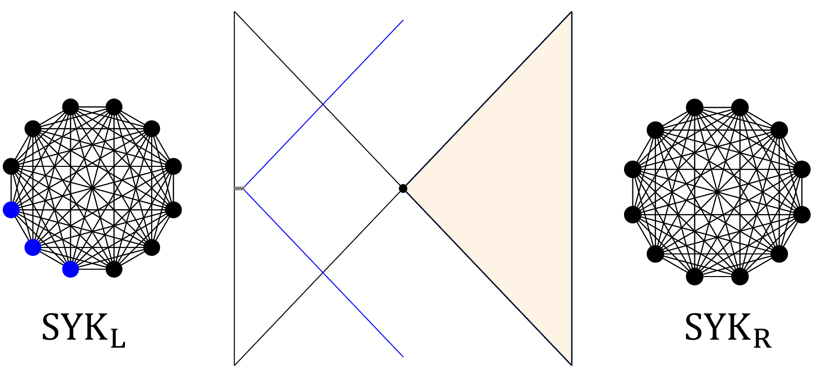
(a) $m<m_{*}$

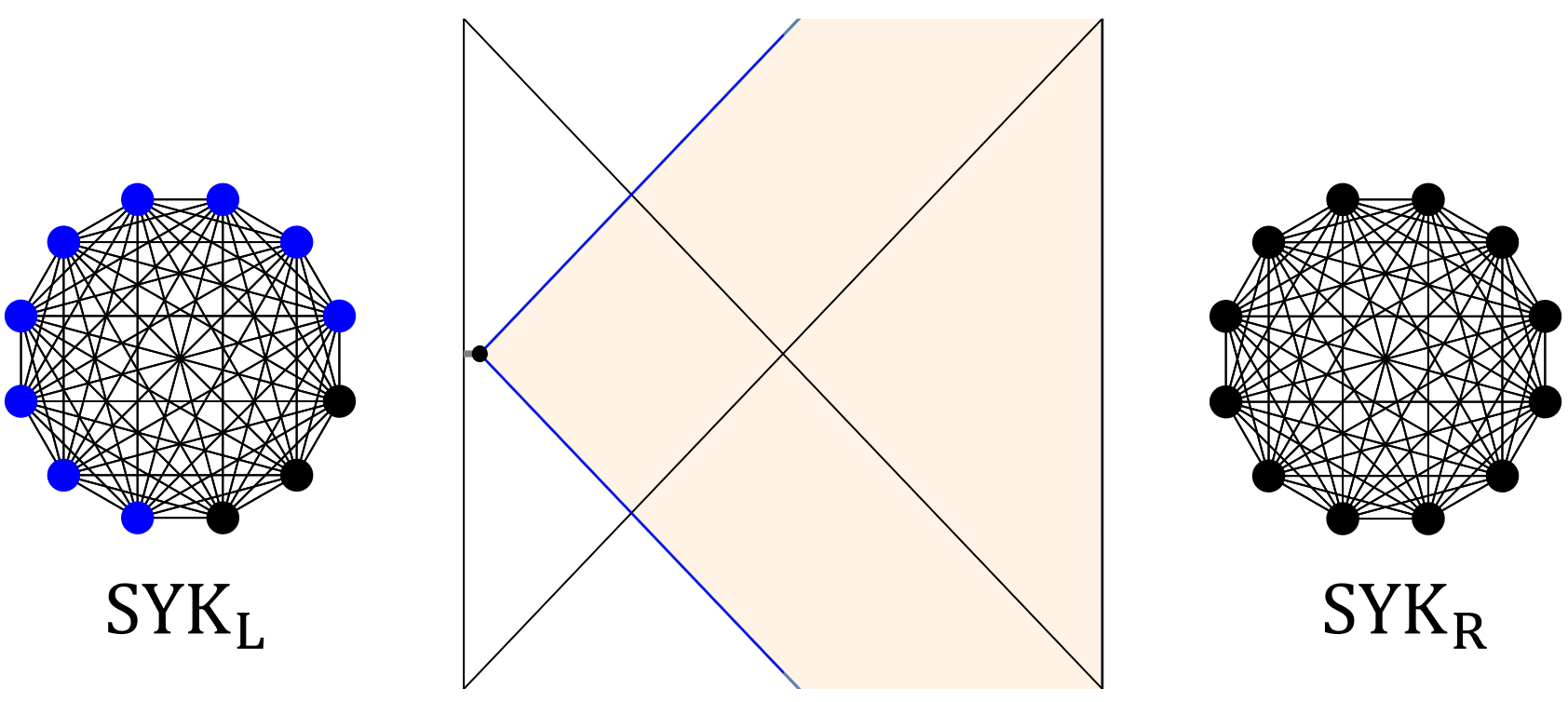
(b) $m>m_{*}$

Figure 1: Measurement-induced entanglement wedge transition. Two copies of the SYK model, denoted by left and right sides, are in a thermofield double state, which is dual to a two-sided eternal $AdS_{2}$ black hole. A subset of the left Majorana fermions are measured, as indicated by blue dots. An end-of-the-world brane is created in the left asymptotic region by the measurement. The entanglement wedge of all of the right Majorana fermions is indicated by the tan region. A small gray segment on the left side indicates the cutoff region (see discussion in Section 3.2). (a) When the number of measured Majorana fermions is less than a critical value, $M/N=m<m_{*}$, the quantum extremal surface is located at the bifurcation surface. (b) When the number of measured Majorana fermions exceeds a critical value, $M/N=m>m_{*}$, the entanglement wedge includes nearly the entire time reversal invariant slice. Note that the transition from (a) to (b) is a sharp phase transition in the bulk von Neumann entropy calculation, while it is a crossover in the SYK Renyi-2 entropy calculation; these are compared in Figure 9.

The main advantage the lower-dimensional toy-models studied here is the large amount of control we have on both sides of the duality. For instance, we are able to explicitly compute quantities in a boundary theory (the SYK model) which can be regarded as a candidate UV completion of the dual bulk theory. We can then compare the results with those obtained in the dual gravitational system in the appropriate limits. On the other hand, thanks to the simplicity of (1+1)-dimensional JT gravity, it is possible to analytically compute the bulk generalized entropy in the presence of bulk matter. Both these features would be remarkably cumbersome to obtain in higher-dimensional theories. Thus, the present analysis allows us to explicitly realize and further extend the constructions described in Antonini:2022sfm , gaining much additional insight into the physical processes taking place in both the boundary and bulk theory when projective measurements are performed. Moreover, the generalized entropy prescription proposed here is a first step towards a more general framework for entanglement in setups that include non-unitary operations such as measurements.

The rest of the paper is organized as follows. In Section 2 we define the SYK model and its TFD state and describe the measurement procedure. We then compute the correlation functions in the post-measurement state using Euclidean path integral techniques in the saddle point approximation (analytically in the large-$q$ limit and numerically for any value of $q$). We then proceed to compute the post-measurement Renyi-2 mutual information between the two sides using a similar path integral procedure. In Section 3 we define the bulk dual theory using JT gravity coupled to matter and study the effects of the projective measurement on the geometry. We compute the post-measurement mutual information between the two sides using the QES prescription and describe the entanglement wedge phase transition and its interpretation in terms of bulk teleportation. In Section 4 we study the teleportation protocol and its fidelity in detail, and make the connection between our results and traversable wormholes. In section 5 we draw our conclusions and discuss future directions. Technical details of our analysis are contained in Appendices A, D, F, and G. In Appendix E we give a simple toy model of the bulk teleportation using Haar random unitaries. In Appendix B we compare our results to the analysis of kourkoulou2017pure ; zhang2020entanglement . In Appendix C we report SYK model results for a measurement performed on subsets of fermions in both sides of the TFD state.

2 Partial measurement of a SYK thermofield double

In this section, we investigate the entanglement structure of a thermofield double state of two copies of the SYK model (the “left” and the “right”) after a measurement is performed on a subset of fermions in one of the two copies (which we will conventionally identify as the “right”). A similar analysis for a measurement performed on a subset of fermions in both sides is reported in Appendix C. We start by defining the measurement operator and describing a Euclidean path integral representation of the measurement procedure. We then introduce the customary bilocal field formulation of the SYK model kitaev ; Sachdev:2015efa ; maldacena2016remarks and study the saddle point solution for the post-measurement system. Finally, we compute the post-measurement Renyi-2 mutual information between the left and the remaining (unmeasured) fermions on the right. We find that the mutual information decreases as we increase the fraction of measured fermions, but is always non-vanishing unless all the right fermions are measured. The analysis of the present section serves also as a benchmark for the results obtained in the holographic dual description of Section 3, where we find an analogous behavior for the mutual information in JT gravity coupled to $N$ copies of a CFT.

2.1 Partial measurement and path integral

The SYK model is defined by the all-to-all interacting Hamiltonian

$$H[\psi]=i^{q/2}\sum_{i_{1}<...<i_{q}}J_{i_{1},...,i_{q}}\psi_{i_{1}}...\psi_{i_{q}},$$ (1)

where $\psi_{i},i=1,...,N$ denotes a Majorana fermion (satisfying $\{\psi_{i},\psi_{j}\}=\delta_{ij}$ and $\psi_{i}^{\dagger}=\psi_{i}$), and $J_{i_{1},...,i_{q}}$ gives the coupling between the Majorana fermions $i_{1},...,i_{q}$. $J_{i_{1},...,i_{q}}$ is a random Gaussian variable with average and variance given by

$$\overline{J_{i_{1},...,i_{q}}}=0,\quad\overline{J_{i_{1},..,i_{q}}J_{i_{1}^{\prime},...,i_{q}^{\prime}}}=\prod_{k=1}^{q}\delta_{i_{k},i_{k}^{\prime}}\frac{J^{2}}{qN^{q-1}},$$ (2)

where $J$ sets the overall interaction strength.

We are interested in studying the post-measurement properties of the TFD state of two copies of the SYK model. The unnormalized TFD state, which is defined in a doubled Hilbert space, is given by

$$|TFD\rangle=e^{-\frac{\beta}{4}(H_{L}+H_{R})}|\infty\rangle$$ (3)

where $\beta$ is a parameter representing the inverse temperature of the thermal system obtained by tracing out one of the two sides, $H_{L}=H[\psi_{L}]$, $H_{R}=H[i\psi_{R}]$ (with $\psi_{L}$ and $\psi_{R}$ Majorana fermion operators on the left and right Hilbert space respectively), and $\ket{\infty}$ is the thermofield double state at infinite temperature defined by $(\psi_{L,i}+i\psi_{R,i})|\infty\rangle=0$ Maldacena:2018lmt .

Given the thermofield double state (3), we now want to perform a projective measurement on $M$ of the $N$ Majorana fermions in the right system. Inspired by the local projective measurement considered in $AdS_{3}/BCFT_{2}$ numasawa2016epr ; Antonini:2022sfm that retains bulk geometry, the measurement operator of interest here will be the fermion parity operator $M_{R,k}$ formed by the $2k-1$ and $2k$ right Majorana fermions in analogy with the analysis of Kourkoulou and Maldacena kourkoulou2017pure :

$$M_{R,k}=-i2\psi_{R,2k-1}\psi_{R,2k}$$ (4)

where the factor of 2 accounts for the chosen normalization of the Majorana fermions and we assume for simplicity that $M$ is an even integer. Intuitively, if we divide Majorana fermions on the right side in pairs $(\psi_{R,2k-1},\psi_{R,2k})_{k=1,...,N/2}$ and identify each pair with a complex fermion $\tilde{\psi}_{R,k}$, the fermion parity (4) corresponds to the Pauli-$Z$ operator $\sigma_{R,k}^{z}$ for the $k$-th complex fermion on the right side. The raising and lowering operators for the complex fermions are then

$$\sigma_{R,k}^{+}=\sqrt{2}\left(\psi_{R,2k-1}+i\psi_{R,2k}\right),\quad\sigma_{R,k}^{-}=\sqrt{2}\left(\psi_{R,2k-1}-i\psi_{R,2k}\right).$$ (5)

To perform a projective measurement on the first $M$ fermions on the right side we must measure the fermi parity (4) for $k=1,...,M/2$. The measurement operators for different $k$ commute. The eigenvalues of each operator are $r_{k}=\pm 1$ . Therefore, the measurement record is given by a string of binary numbers $\textbf{r}=(r_{1},...,r_{M/2})$. In our analysis below we will study how properties of the post-measurement state change when varying the number of measurement operators applied on the right side—given by $M/2$. More precisely, since we are interested in studying the SYK model in the large-$N$ limit (where it admits a semiclassical bulk dual spacetime), we define $m\equiv M/N$, take the large-$N$ limit keeping $m$ fixed, and then vary the value of $m$.

Suppose we measure the fermion parity (4) for $k=1,...,M/2$ in the TFD state (3) and get a measurement outcome $\textbf{r}=(r_{1},...,r_{M/2})$. The post-measurement state $|R_{\textbf{r}}(m)\rangle$ for the $M$ measured right Majorana fermions is an eigenstate of all the $M/2$ fermion parity operators :

$$M_{R,k}|R_{\textbf{r}}(m)\rangle=r_{k}|R_{\textbf{r}}(m)\rangle,\quad k=1,...,M/2.$$ (6)

Using the raising and lowering operators introduced in equation (5), equation (6) can be rewritten in the form

$$\psi_{R,2k-1}|R_{\textbf{r}}(m)\rangle=-ir_{k}\psi_{R,2k}|R_{\textbf{r}}(m)\rangle,\quad k=1,...,M/2,$$ (7)

which will be useful for identifying the correct boundary conditions in the path integral formalism. Therefore, the full post-measurement (unnormalized) state of the two-sided system can be obtained by inserting the projection operator $|R_{\textbf{r}}(m)\rangle\langle R_{\textbf{r}}(m)|$:

$$|\Psi_{\textbf{r}}(m)\rangle=\left(\mathds{1}^{(1-m)}\otimes|R_{\textbf{r}}(m)\rangle\langle R_{\textbf{r}}(m)|\right)|TFD\rangle$$ (8)

where we use $\mathds{1}^{(1-m)}$ to denote the identity operator acting on the unmeasured Majorana fermions on the right side . The Born probability of observing this state is $p_{\textbf{r}}(m)=\frac{\langle\Psi_{\textbf{r}}(m)|\Psi_{\textbf{r}}(m)\rangle}{\langle TFD|TFD\rangle}$. Note that the simultaneous eigenstates of all the fermion parity operators (4) for $k=1,...,M/2$ form a complete basis of the measured subspace, i.e.

$$\sum_{\textbf{r}}|R_{\textbf{r}}(m)\rangle\langle R_{\textbf{r}}(m)|=\mathds{1}^{(m)},$$ (9)

which leads to $\sum_{\textbf{r}}p_{\textbf{r}}(m)=1$, as expected.

Now that we have fully characterized the measurement operator and the post-measurement state, we can compute the amplitude $\overline{\langle\Psi_{\textbf{r}}(m)|\Psi_{\textbf{r}}(m)\rangle}$ using a Euclidean path integral representation. Here, as above, the overline indicates averaging over the Gaussian couplings (2). The amplitude can be written as

$$\begin{aligned} \overline{\langle\Psi_{\textbf{r}}(m)|\Psi_{\textbf{r}}(m)\rangle}&=\overline{\langle TFD|\left(|R_{\textbf{r}}(m)\rangle\langle R_{\textbf{r}}(m)|\right)|TFD\rangle}\\ &=\overline{\text{Tr}_{R}\left[e^{-\beta H_{R}}|R_{\textbf{r}}(m)\rangle\langle R_{\textbf{r}}(m)|\right]}=\int D\psi e^{-I},\end{aligned}$$ (10)

where in the second equality we used the properties of the TFD state (3), $\text{Tr}_{R}$ denotes the trace over the right system, and the action appearing in the Euclidean path integral is given by 

$$-I=-\int d\tau\sum_{j}\frac{1}{2}\psi_{j}(\tau)\partial_{\tau}\psi_{j}(\tau)+\int d\tau_{1}d\tau_{2}\frac{J^{2}}{2qN^{q-1}}\left(\sum_{j}\psi_{j}(\tau_{1})\psi_{j}(\tau_{2})\right)^{q}.$$ (11)

The insertion of the projection operator $|R_{\textbf{r}}(m)\rangle\langle R_{\textbf{r}}(m)|$ in the trace corresponds to the following boundary conditions in the path integral:

$$\begin{aligned} &\psi_{2k-1}(0)=-ir_{k}\psi_{2k}(0),\quad\psi_{2k-1}(\beta)=ir_{k}\psi_{2k}(\beta),\quad k=1,...,M/2,\\ &\psi_{M+j}(0)=-\psi_{M+j}(\beta),\quad j=1,...,N-M\end{aligned}$$ (12)

where we inserted the projection operator at Euclidean time $\tau=0$ (corresponding to the right system). The boundary conditions for the measured Majorana fermions—i.e. $\psi_{k}$ with $1\leq k\leq M$—reported in the first line of equation (12) can be obtained from equation (7) and its complex conjugate . On the other hand, the unmeasured Majorana fermions $\psi_{k}$ with $M+1\leq k\leq N$ satisfy the conventional anti-periodic boundary conditions for fermionic fields, reported in the second line of equation (12). The boundary conditions on the Euclidean time circle are illustrated in Fig. 2.

If $m=0$—which means no fermions are measured— the path integral clearly computes the usual thermal partition function with inverse temperature $\beta$. On the other hand, if $m=1$—which means that the whole right system is measured—the path integral can be interpreted as preparing a Kourkoulou-Maldacena state kourkoulou2017pure at $\tau=\beta/2$ (see Appendix B).

Figure 2: Different boundary conditions for Majorana fields in the imaginary time contour. (a) The measurement operator $|R_{\textbf{r}}(m)\rangle\langle R_{\textbf{r}}(m)|$ is inserted on the contour at $\tau=0$, which is indicated by two small triangles, for $\psi_{i},i=1,...,M$. (b) The conventional contour for $\psi_{j+M},j=1,...,N-M$.

It is now useful to introduce bilocal collective fields, in terms of which the equations of motion derived in the saddle point approximation of the Euclidean path integral are substantially simplified kitaev ; Sachdev:2015efa ; maldacena2016remarks . The form of the boundary conditions (12) suggests that we should introduce different types of bilocal fields. First, we introduce the “diagonal” bilocal fields

$$\begin{aligned} &\tilde{G}_{11}(\tau_{1},\tau_{2})=\frac{2}{M}\sum_{k=1}^{M/2}\psi_{2k-1}(\tau_{1})\psi_{2k-1}(\tau_{2}),\qquad\tilde{G}_{22}(\tau_{1},\tau_{2})=\frac{2}{M}\sum_{k=1}^{M/2}\psi_{2k}(\tau_{1})\psi_{2k}(\tau_{2}),\\ &\tilde{G}_{33}(\tau_{1},\tau_{2})=\frac{1}{N-M}\sum_{j=1}^{N-M}\psi_{M+j}(\tau_{1})\psi_{M+j}(\tau_{2}).\end{aligned}$$ (13)

For later convenience, we also introduce the following “off-diagonal” bilocal fields (similar to the ones introduced in kourkoulou2017pure ):

$$\tilde{G}_{12}(\tau_{1},\tau_{2})=\frac{2}{M}\sum_{k=1}^{M/2}r_{k}\psi_{2k-1}(\tau_{1})\psi_{2k}(\tau_{2}),\quad\tilde{G}_{21}(\tau_{1},\tau_{2})=\frac{2}{M}\sum_{k=1}^{M/2}r_{k}\psi_{2k}(\tau_{1})\psi_{2k-1}(\tau_{2}).$$ (14)

In terms of these bilocal fields (the arguments of which are in the range $\tau_{1,2}\in(0,\beta)$), the large-$N$ action becomes

$$-I=\int d\tau_{1}d\tau_{2}\Big{[}-\frac{1}{2}\Big{(}\sum_{k=1}^{M/2}\psi_{2k-1}(\tau_{1})(\partial-\tilde{\Sigma}_{11})\psi_{2k-1}(\tau_{2})+\sum_{k=1}^{M/2}\psi_{2k}(\tau_{1})(\partial-\tilde{\Sigma}_{22})\psi_{2k}(\tau_{2})$$

$$+\sum_{j=M+1}^{N}\psi_{j}(\tau_{1})(\partial-\tilde{\Sigma}_{33})\psi_{j}(\tau_{2})\Big{)}-\frac{1}{2}\left(\frac{M}{2}\tilde{\Sigma}_{11}\tilde{G}_{11}+\frac{M}{2}\tilde{\Sigma}_{22}\tilde{G}_{22}+(N-M)\tilde{\Sigma}_{33}\tilde{G}_{33}\right)$$

$$+\frac{J^{2}}{2qN^{q-1}}\left(\frac{M}{2}\tilde{G}_{11}(\tau_{1},\tau_{2})+\frac{M}{2}\tilde{G}_{22}(\tau_{1},\tau_{2})+(N-M)\tilde{G}_{33}(\tau_{1},\tau_{2})\right)^{q}\Big{]},$$ (15)

where $\partial=\delta(\tau_{1}-\tau_{2})\partial_{\tau_{2}}$, and we have introduced the Lagrange multiplier fields $\tilde{\Sigma}_{11}(\tau_{1},\tau_{2})$, $\tilde{\Sigma}_{22}(\tau_{1},\tau_{2})$ and $\tilde{\Sigma}_{33}(\tau_{1},\tau_{2})$ (which play the role of the self-energy). It is easy to check that integrating out the Lagrange multiplier fields enforces the definitions (13) of the bilocal fields.

Before deriving the equations of motion, it is useful to define a new Majorana field zhang2020entanglement

$$\chi_{k}(s)=\begin{cases}\psi_{2k-1}(s),\quad&0<s<\beta,\\ ir_{k}\psi_{2k}(2\beta-s),\quad&\beta<s<2\beta.\end{cases}$$ (16)

In the rest of the present subsection and in the next subsection we denote by $s$ coordinates in the range $(0,2\beta)$ and by $\tau$ coordinates in the range $(0,\beta)$. The advantage of introducing this new field is that the boundary conditions (12) reduce to the conventional anti-periodic boundary conditions for $\chi_{k}(s)$, i.e. $\chi_{k}(0)=-\chi_{k}(2\beta)$. In terms of the new field $\chi_{k}(s)$ the first line of equation (2.1) becomes

$$-\frac{1}{2}\int_{0}^{2\beta}ds_{1}\int_{0}^{2\beta}ds_{2}\chi_{k}(s_{1})\left(\delta(s_{1}-s_{2})\partial_{s_{2}}-\hat{\tilde{\Sigma}}(s_{1},s_{2})\right)\chi_{k}(s_{2}),$$ (17)

where we used $r_{k}^{2}=1$ and introduced a compact notation for the self-energy $\hat{\tilde{\Sigma}}(s_{1},s_{2})$ (with $0<s_{1,2}<2\beta$)

$$\hat{\tilde{\Sigma}}(s_{1},s_{2})=\left[\begin{array}[]{cccc}\tilde{\Sigma}_{11}(s_{1},s_{2})&0\\ 0&-\tilde{\Sigma}_{22}(2\beta-s_{1},2\beta-s_{2})\end{array}\right].$$ (20)

In this matrix notation, the range of the $s_{i}$ coordinates for the $\hat{\tilde{\Sigma}}_{a_{1}a_{2}}(s_{1},s_{2})$ element is $(a_{i}-1)\beta<s_{i}<a_{i}\beta$ with $a_{i}=1,2$, for $i=1,2$, respectively. More explicitly, $\hat{\tilde{\Sigma}}_{11}(s_{1},s_{2})=\tilde{\Sigma}_{11}(s_{1},s_{2})$ with $0<s_{1},s_{2}<\beta$ and $\hat{\tilde{\Sigma}}_{22}(s_{1},s_{2})=-\tilde{\Sigma}_{22}(2\beta-s_{1},2\beta-s_{2})$ with $\beta<s_{1},s_{2}<2\beta$. The ranges $0<s_{1}<\beta$, $\beta<s_{2}<2\beta$ and $\beta<s_{1}<2\beta$, $0<s_{2}<\beta$ correspond to the (vanishing) off-diagonal elements $\hat{\tilde{\Sigma}}_{12}(s_{1},s_{2})$ and $\hat{\tilde{\Sigma}}_{21}(s_{1},s_{2})$, respectively.

Now both $\psi_{j},j=M+1,...,N$ and $\chi_{k},k=1,...,M/2$ satisfy the conventional anti-periodic boundary conditions typical of fermionic fields. We can then integrate out the Majorana fermions to get

$$-\frac{I}{N} = \frac{m}{2}\log\text{Pf}\left(\partial-\hat{\tilde{\Sigma}}\right)+(1-m)\log\text{Pf}(\partial-\tilde{\Sigma}_{33})$$ (22)

$$-\int d\tau_{1}d\tau_{2}\frac{1}{2}\left(\frac{m}{2}\tilde{\Sigma}_{11}\tilde{G}_{11}+\frac{m}{2}\tilde{\Sigma}_{22}\tilde{G}_{22}+(1-m)\tilde{\Sigma}_{33}\tilde{G}_{33}\right)$$

$$+\int d\tau_{1}d\tau_{2}\frac{J^{2}}{2q}\left(\frac{m}{2}\tilde{G}_{11}+\frac{m}{2}\tilde{G}_{22}+(1-m)\tilde{G}_{33}\right)^{q}$$

where Pf indicates the Pfaffian. Owing to the large $N$ structure of the action, we can derive the equations of motion in the saddle point approximation, which are given by the Schwinger-Dyson equations (here and in the following we drop the $\tilde{}$ to indicate on-shell solutions)

$$\hat{G}(s_{1},s_{2}) = \left(\partial-\hat{\Sigma}\right)^{-1}(s_{1},s_{2}),\quad G_{33}(\tau_{1},\tau_{2})=(\partial-\Sigma_{33})^{-1}(\tau_{1},\tau_{2}),$$ (23)

$$\Sigma_{ii}(\tau_{1},\tau_{2}) = J^{2}\left(\frac{m}{2}G_{11}(\tau_{1},\tau_{2})+\frac{m}{2}G_{22}(\tau_{1},\tau_{2})+(1-m)G_{33}(\tau_{1},\tau_{2})\right)^{q-1},\quad i=1,2,3.$$

where we have introduced a compact notation for $\hat{G}$ analogous to the one introduced in equation (20) for the self-energy:

$$\hat{G}(s_{1},s_{2})=\left[\begin{array}[]{cccc}G_{11}(s_{1},s_{2})&iG_{12}(s_{1},2\beta-s_{2})\\ iG_{21}(2\beta-s_{1},s_{2})&-G_{22}(2\beta-s_{1},2\beta-s_{2})\end{array}\right].$$ (26)

Note that for the off-diagonal components, $\hat{G}_{a_{1}a_{2}}(s_{1},s_{2})$ with $a_{1}\neq a_{2}$, the matrix notation introduced after equation (20) implies that the ranges of the $s_{1}$ and $s_{2}$ coordinates are different (i.e. $0<s_{1}<\beta$, $\beta<s_{2}<2\beta$ for $\hat{G}_{12}$ and $\beta<s_{1}<2\beta$, $0<s_{2}<\beta$ for $\hat{G}_{21}$). It is not hard to see that $\hat{G}(s_{1},s_{2})=\frac{2}{M}\sum_{k=1}^{M/2}\chi_{k}(s_{1})\chi_{k}(s_{2})$.

$\hat{G}$ and $G_{33}$ are on-shell Green’s functions. In the next subsection, we will compute $\hat{G}$ and $G_{33}$ by solving the Schwinger-Dyson equations (23) analytically in the large-$q$ limit and numerically for any value of $q$.

2.2 Saddle point solution

The action (11) is $O(N)$-symmetric. In particular, it is invariant under the action of a subgroup of $O(N)$, the “Flip group” kourkoulou2017pure , the elements of which flip the sign of any number of even-indexed Majorana fermions. In other words, the action of an element of the Flip group is given by $\psi_{2k-1}\rightarrow\psi_{2k-1},\psi_{2k}\rightarrow-\psi_{2k}$ for one or more given values of $k$ with $1\leq k\leq N/2$. In terms of the complex fermions $\tilde{\psi}_{k}$ associated with pairs of Majorana fermions, an element of the Flip group flips the sign of one or more spins. Note that both the diagonal and the-off diagonal bilocal fields (13) and (14) are invariant under the Flip group as well as the on-shell Green’s functions.

The invariance under the Flip group clearly implies that all our results are independent of the measurement outcome $\textbf{r}=(r_{1},...,r_{M/2})$: the Flip group acting on any number of the first $M$ Majorana fermions can map a given measurement outcome to any other measurement outcome. One consequence of this invariance is that the on-shell solutions $\hat{G}(s_{1},s_{2})$ and $G_{33}(\tau_{1},\tau_{2})$ in our setup involving measurement are related to the thermal Green’s function $G_{th}(\tau_{1},\tau_{2})$. In fact, the on-shell Green’s function $G_{11}(\tau_{1},\tau_{2})$ can be written as

$$G_{11}(\tau_{1},\tau_{2}) = \frac{2}{M}\sum_{k}\frac{1}{Z}\text{Tr}\left[e^{-\beta H[\psi]}\mathcal{T}\left(\psi_{2k-1}(\tau_{1})\psi_{2k-1}(\tau_{2})\right)|R_{\textbf{r}}(m)\rangle\langle R_{\textbf{r}}(m)|\right],$$ (27)

where $Z=\text{Tr}\left[e^{-\beta H[\psi]}|R_{\textbf{s}}(m)\rangle\langle R_{\textbf{s}}(m)|\right]$ is the normalization factor, $\psi(\tau)=e^{H[\psi]\tau}\psi e^{-H[\psi]\tau}$, and $\mathcal{T}$ denotes imaginary time ordering. Using the invariance under measurement outcome, we can then write

$$G_{11}(\tau_{1},\tau_{2}) = \frac{2}{M}\sum_{k}\frac{1}{Z}\left(\frac{1}{2^{M/2}}\sum_{\textbf{r}}\text{Tr}\left[e^{-\beta H[\psi]}\mathcal{T}\left(\psi_{2k-1}(\tau_{1})\psi_{2k-1}(\tau_{2})\right)|R_{\textbf{r}}(m)\rangle\langle R_{\textbf{r}}(m)|\right]\right)$$ (28)

$$= \frac{2}{M}\sum_{k}\frac{\text{Tr}\left[e^{-\beta H[\psi]}\mathcal{T}\left(\psi_{2k-1}(\tau_{1})\psi_{2k-1}(\tau_{2})\right)\right]}{\text{Tr}\left[e^{-\beta H[\psi]}\right]}$$

$$= \frac{1}{N}\sum_{i}\frac{\text{Tr}\left[e^{-\beta H[\psi]}\mathcal{T}\left(\psi_{i}(\tau_{1})\psi_{i}(\tau_{2})\right)\right]}{\text{Tr}\left[e^{-\beta H[\psi]}\right]}=G_{th}(\tau_{1},\tau_{2})$$

where to go from the first to the second line we have used the completeness relation for the measured subspace $\sum_{\textbf{r}}|R_{\textbf{r}}(m)\rangle\langle R_{\textbf{r}}(m)|=\mathds{1}^{(m)}$ and $Z=\frac{1}{2^{M/2}}\sum_{\textbf{r}}\text{Tr}\left[e^{-\beta H[\psi]}|R_{\textbf{r}}(m)\rangle\langle R_{\textbf{r}}(m)|\right]=\frac{1}{2^{M/2}}\text{Tr}\left[e^{-\beta H[\psi]}\right]$. The equality leading from the second to the third line is true in virtue of the $O(N)$ symmetry of the model. An analogous relation can be obtained for $G_{22}(\tau_{1},\tau_{2})$ and $G_{33}(\tau_{1},\tau_{2})$. Therefore, $G_{ii},i=1,2,3$ are all given by the usual imaginary time correlation.

The Schwinger-Dyson equations (23) can then be rewritten in a simpler form 

$$\hat{G}=(\partial-\hat{\Sigma})^{-1},\quad\hat{\Sigma}(s_{1},s_{2})=\frac{\mathcal{J}^{2}}{q}P(s_{1},s_{2})[2\hat{G}(s_{1},s_{2})]^{q-1},$$ (29)

where we defined $\mathcal{J}^{2}=qJ/2^{q-1}$ for later convenience and

$$P(s_{1},s_{2})=\theta(\beta-s_{1})\theta(\beta-s_{2})+\theta(s_{1}-\beta)\theta(s_{2}-\beta).$$ (30)

The boundary conditions now read

$$\hat{G}(s,s)=\frac{1}{2},\quad\hat{G}(s_{1},s_{2})=-\hat{G}(s_{2},s_{1}),\quad\hat{G}(s_{1}+2\beta,s_{2})=-\hat{G}(s_{1},s_{2}).$$ (31)

The first and second equations are a consequence of the commutation relations and the definition of the time ordering operator, whereas the third condition implements the anti-periodic boundary conditions for the fermionic field $\chi(s)$.

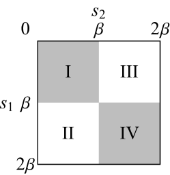
Figure 3: The domain of the bilocal Green’s function $\hat{G}(s_{1},s_{2})$. $P(s_{1},s_{2})$ is nonzero in the shaded regions I and IV. According to our matrix notation, $\hat{G}_{11}(s_{1},s_{2})=G_{11}(s_{1},s_{2})$ denotes the Green’s function in region I, $\hat{G}_{21}(s_{1},s_{2})=iG_{21}(2\beta-s_{1},s_{2})$ denotes the Green’s function in region II, $\hat{G}_{12}(s_{1},s_{2})=iG_{12}(s_{1},2\beta-s_{2})$ denotes the Green’s function in region III, and $\hat{G}_{22}(s_{1},s_{2})=-G_{22}(2\beta-s_{1},2\beta-s_{1})$ denotes the Green’s function in region IV.

The Schwinger-Dyson equations can be solved analytically in the large-$q$ limit maldacena2016remarks . Using the ansatz $\hat{G}(s_{1},s_{2})=\hat{G}_{0}(s_{1},s_{2})\left(1+\frac{1}{q}g(s_{1},s_{2})+...\right)$, where we suppressed terms of higher order in $q$ and introduced the bare propagator

$$\hat{G}_{0}(s_{1},s_{2})=\frac{1}{2}\left[\begin{array}[]{cccc}\text{sgn}(s_{1}-s_{2})&-1\\ 1&\text{sgn}(s_{1}-s_{2})\end{array}\right],$$ (34)

the Schwinger-Dyson equations (29) at leading order in $q$ give an equation for $g(s_{1},s_{2})$ maldacena2016remarks :

$$\partial_{s_{1}}\partial_{s_{2}}[\hat{G}_{0}(s_{1},s_{2})g(s_{1},s_{2})]=\mathcal{J}^{2}P(s_{1},s_{2})[2\hat{G}_{0}(s_{1},s_{2})]^{q-1}e^{g(s_{1},s_{2})}.$$ (35)

Note that the measurement introduces a factor $P(s_{1},s_{2})$ on the right-hand side which is not present in the conventional Liouville equation maldacena2016remarks . Given the expression (30) for $P(s_{1},s_{2})$, we can divide the domain into four regions as shown in Fig. 3. In region I and IV, the Liouville equation (35) takes the form 

$$\partial_{s_{1}}\partial_{s_{2}}g(s_{1},s_{2})=2\mathcal{J}^{2}e^{g(s_{1},s_{2})}.$$ (36)

The relationship (28) between the diagonal Green’s functions in our setup and the thermal Green’s function implies that we can assume the diagonal elements of $\hat{G}(s_{1},s_{2})$ (i.e. the Green’s function in regions I and IV) are time translation invariant. Therefore in region I and IV, $g(s_{1},s_{2})=g(s_{12})$ where $s_{12}\equiv s_{1}-s_{2}$. The solution of the Liouville equation is then

$$g_{\text{I}}(s_{12})=g_{\text{IV}}(s_{12})=2\log\left[\frac{\sin\gamma}{\sin(\alpha|s_{12}|+\gamma)}\right]$$ (37)

where $\alpha=\mathcal{J}\sin\gamma$ and $\gamma$ is a constant to be determined by imposing the anti-periodic boundary condition. At leading order in $q$ we then obtain the following result for the diagonal elements of $\hat{G}(s_{1},s_{2})$:

$$\hat{G}_{11}(s_{1},s_{2})=\hat{G}_{22}(s_{1},s_{2})=\frac{1}{2}\text{sgn}(s_{12})\left(\frac{\sin\gamma}{\sin(\alpha|s_{12}|+\gamma)}\right)^{2/q}.$$ (38)

In regions II and III, the Liouville equation (35) takes the form $\partial_{s_{1}}\partial_{s_{2}}g(s_{1},s_{2})=0$, which is solved by the ansatz $g(s_{1},s_{2})=f_{1}(s_{1})+f_{2}(s_{2})$. The form of $f_{1}(s_{1})$ and $f_{2}(s_{2})$ can be obtained by matching the solutions for $\hat{G}(s_{1},s_{2})$ at the boundaries between regions I,IV and regions II,III. This yields the following off-diagonal elements of $\hat{G}(s_{1},s_{2})$:

$$\begin{aligned} &\hat{G}_{21}(s_{1},s_{2})=\frac{1}{2}\left(\frac{\sin\gamma}{\sin(\alpha(s_{1}-\beta)+\gamma)}\frac{\sin\gamma}{\sin(\alpha(\beta-s_{2})+\gamma)}\right)^{2/q},\\ &\hat{G}_{12}(s_{1},s_{2})=-\frac{1}{2}\left(\frac{\sin\gamma}{\sin(\alpha(s_{2}-\beta)+\gamma)}\frac{\sin\gamma}{\sin(\alpha(\beta-s_{1})+\gamma)}\right)^{2/q}.\end{aligned}$$ (39)

Finally, imposing the anti-periodic boundary condition $\hat{G}(s_{1}+2\beta,s_{2})=-\hat{G}(s_{1},s_{2})$, the constant $\gamma$ is implicitly determined by

$$\gamma+\frac{\mathcal{J}\beta\sin\gamma}{2}=\frac{\pi}{2}.$$ (40)

Note that our results for the off-diagonal Green’s function (39) are in agreement with the $m=1$ results of kourkoulou2017pure .

(a) $G_{33}$

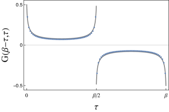
(b) $G_{11,22}$

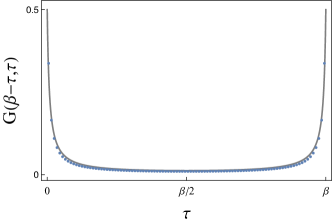
(c) $G_{21}$

Figure 4: A comparison between numerical (represented by blue dots) and large-$q$ analytical (represented by gray curves) solutions for the diagonal components of the Green’s function. The parameters are $\beta\mathcal{J}=20$, $q=4$. The imaginary time contour with length $\beta$ is discretized into $100$ intervals. (a) The unmeasured Majorana fermions’ Green’s function $G_{33}(\tau_{1},\tau_{2})$. (b) The measured Majorana fermions’ Green’s functions $G_{11}(\tau_{1},\tau_{2})$, $G_{22}(\tau_{1},\tau_{2})$. Note that $G_{11}(\tau_{1},\tau_{2})=G_{22}(\tau_{1},\tau_{2})=G_{33}(\tau_{1},\tau_{2})$ as expected by the flip symmetry argument in equation (28). (c) The measured Majorana fermions’ Green’s function $G_{21}(\tau_{1},\tau_{2})$.

Alternatively, the Schwinger-Dyson equation (29) can be solved numerically by iteration for any value of $q$. Given that our results are independent of the measurement outcome, we take for simplicity $r_{k}=1$ for all $k=1,...,M/2$. A comparison of the numerical results with the large $q$ solution described above is shown in Fig. 4, where the dots are numerical results and the gray curves are the analytical large-$q$ solutions derived above. Note that, as expected, the numerical solutions for the diagonal Green’s functions of the measured Majorana fermions $G_{11}(\tau_{1},\tau_{2})$, $G_{22}(\tau_{1},\tau_{2})$ and the ummeasured Majorana fermions $G_{33}(\tau_{1},\tau_{2})$ are identical.

2.3 Mutual information

In order to set the stage for the holographic calculation carried out in Section 3, we now compute the post-measurement Renyi-2 mutual information between the left side and the unmeasured Majorana fermions on the right side. The SYK mutual information computed in the present subsection will serve as a benchmark to test our results for the holographic mutual information, which will give us information about the effect of the measurement on the wormhole dual to the SYK thermofield double state. The choice of computing the Renyi-2 mutual information in the SYK setup rather than the Von Neumann mutual information is due to the fact that it can be easily computed in the saddle point approximation using a Euclidean path integral for two replicas of our system with appropriate boundary conditions. The Renyi-2 entropy is also known to provide a good qualitative approximation of the von Neumann entropy for the SYK model (see the discussion and comparison between Renyi-2 entropy and von Neumann entropy from exact diagonalization liu2018quantum in Ref. zhang2020subsystem ). This is confirmed by our comparison between the SYK Renyi-2 mutual information and the holographic von Neumann entropy computed in the bulk dual setup in Section 3.

As we discussed in the previous subsection, the unnormalized post-measurement state of the two-sided system is $|\Psi_{\textbf{r}}(m)\rangle$ given by (8), and the corresponding unnormalized density matrix is $\Psi_{\textbf{r}}(m)\equiv|\Psi_{\textbf{r}}(m)\rangle\langle\Psi_{\textbf{r}}(m)|$. Because $|\Psi_{\textbf{r}}(m)\rangle$ is a pure state, we have $S_{L}(\Psi_{\textbf{r}}(m))=S_{R}(\Psi_{\textbf{r}}(m))$, and $S_{LR}(\Psi_{\textbf{r}}(m))=0$. Here $S_{L}$ ($S_{R}$) denotes the entanglement entropy of the left (right) side, and $S_{LR}$ denotes the entanglement entropy of the full two-sided system. Therefore, the mutual information is twice the entanglement entropy of the left system

$$I_{LR}(\Psi_{\textbf{r}}(m))=S_{L}(\Psi_{\textbf{r}}(m))+S_{R}(\Psi_{\textbf{r}}(m))-S_{LR}(\Psi_{\textbf{r}}(m))=2S_{L}(\Psi_{\textbf{r}}(m)).$$ (41)

We focus our attention on the Renyi-2 entanglement entropy—denoted by $S^{(2)}(\Psi_{\textbf{r}}(m))$. This can be obtained via numerical evaluation of a path integral for two replicas of our system, with appropriate boundary conditions which we will derive below. The Renyi-2 entropy of the left system is defined by

$$e^{-S_{L}^{(2)}(\Psi(m))}=\frac{\overline{\text{Tr}_{L}\left[(\text{Tr}_{R}[\Psi(m)])^{2}\right]}}{\overline{\left(\text{Tr}[\Psi(m)]\right)^{2}}},$$ (42)

where we used the fact that disorder-averaging the ratio is equivalent to disorder-averaging the numerator and denominator separately up to $1/N$-suppressed corrections. We have also omitted the subscript r indicating the measurement outcome due to the invariance under measurement outcome discussed above. In particular, in the following calculation we set $r_{k}=1,k=1,...,M/2$ for simplicity.

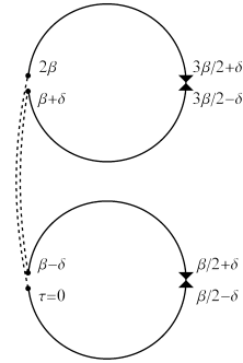
(a) $i=1,...,M$

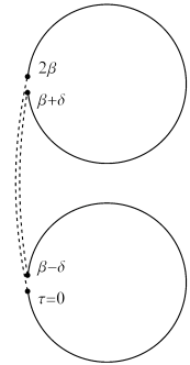
(b) $i=M+1,...,N$

Figure 5: Imaginary time contour $\tau\in(0,2\beta)$ for the Euclidean path integral computing the numerator of equation (42). The points $\tau=0$, $\beta\pm\delta$, $\beta/2\pm\delta$, $3\beta/2\pm\delta$ and $2\beta$ where boundary conditions must be imposed are labeled in the figure. The twist operator inserted in the left system is indicated by the dashed line. (a) The effect of the measurement operator on $\psi_{i},i=1,...,M$ is indicated by the triangles, corresponding to the second and third lines of the boundary conditions (45). At the insertion point of the twist operator, the boundary conditions are given by the first line of (45). (b) There is no measurement operator for $\psi_{i},i=M+1,...,N$. The boundary conditions are then simply set by the first line of  (45).

Equation (42) can be expressed in terms of Euclidean path integrals computing the numerator and denominator separately. Because the Renyi-2 entropy involves the square of the density matrix, we extend the imaginary time contour to $\tau\in(0,2\beta)$ with $\tau\in(0,\beta)$ corresponding to the first replica and $\tau\in(\beta,2\beta)$ corresponding to the second replica. With a change of notation from the previous subsections, we consider the left system to be at $\tau=0,\beta,2\beta$ (for the two replicas) and the right system where the measurement is performed to be at $\tau=\beta/2,3\beta/2$. When computing the numerator of (42), a twist operator must be inserted in the left system, setting anti-periodic boundary conditions at $\tau=0,2\beta$ for the Majorana fermions with period $2\beta$; there is no twist operator for the denominator. Additionally, as in the previous subsections, the measurement operator inserted in the right side sets different boundary conditions for measured and unmeasured Majorana fermions. See Fig. 5 for a representation of the boundary conditions in the path integral computing the numerator of (42).

The path integral for the numerator reads

$$\overline{\text{Tr}_{L}\left[(\text{Tr}_{R}[\Psi(m)])^{2}\right]}=\int D\psi e^{-I},$$ (43)

where the action is given by

$$-I=-\int_{0}^{2\beta}d\tau\sum_{j}\frac{1}{2}\psi_{j}(\tau)\partial_{\tau}\psi_{j}(\tau)+\int_{0}^{2\beta}d\tau_{1}\int_{0}^{2\beta}d\tau_{2}\frac{J^{2}}{2qN^{q-1}}\left(\sum_{j}\psi_{j}(\tau_{1})\psi_{j}(\tau_{2})\right)^{q},$$

and the boundary conditions are

$$\begin{aligned} &\psi_{i}(0)=-\psi_{i}(2\beta),\quad\psi_{i}(\beta_{-})=\psi_{i}(\beta_{+}),\quad i=1,...,N,\\ &\psi_{2k-1}\left(\frac{\beta_{-}}{2}\right)=i\psi_{2k}\left(\frac{\beta_{-}}{2}\right),\quad\psi_{2k-1}\left(\frac{\beta_{+}}{2}\right)=-i\psi_{2k}\left(\frac{\beta_{+}}{2}\right),\quad k=1,...,M/2,\\ &\psi_{2k-1}\left(\frac{3\beta_{-}}{2}\right)=i\psi_{2k}\left(\frac{3\beta_{-}}{2}\right),\quad\psi_{2k-1}\left(\frac{3\beta_{+}}{2}\right)=-i\psi_{2k}\left(\frac{3\beta_{+}}{2}\right),\quad k=1,...,M/2.\end{aligned}$$ (45)

Here we used $\beta_{\pm}$ as a shorthand notation to indicate that the quantity in parenthesis is shifted by an infinitesimal positive number $\delta$ (for instance, $3\beta_{\pm}/2=3\beta/2\pm\delta$). The first line of equation (45) is a consequence of the presence of the twist operator in the left system; the second and third lines are a consequence of the insertion of the measurement operator (4) in the right side for $k=1,...,M/2$ (see Fig. 5 for an illustration).

Similarly, the denominator of equation (42) can also be represented by a path integral with the same action (2.3). The only difference is in the boundary conditions. In fact, the absence of a twist operator implies that the boundary conditions for the denominator read

$$\begin{aligned} &\psi_{i}(0)=-\psi_{i}(\beta_{-}),\quad\psi_{i}(\beta_{+})=-\psi_{i}(2\beta),\quad i=1,...,N,\\ &\psi_{2k-1}\left(\frac{\beta_{-}}{2}\right)=i\psi_{2k}\left(\frac{\beta_{-}}{2}\right),\quad\psi_{2k-1}\left(\frac{\beta_{+}}{2}\right)=-i\psi_{2k}\left(\frac{\beta_{+}}{2}\right),\quad k=1,...,M/2,\\ &\psi_{2k-1}\left(\frac{3\beta_{-}}{2}\right)=i\psi_{2k}\left(\frac{3\beta_{-}}{2}\right),\quad\psi_{2k-1}\left(\frac{3\beta_{+}}{2}\right)=-i\psi_{2k}\left(\frac{3\beta_{+}}{2}\right),\quad k=1,...,M/2.\end{aligned}$$ (46)

The next step is to rewrite the large-$N$ action in terms of bilocal fields analogous to the ones defined in equations (13) and (14), but with arguments in the range $\tau_{1,2}\in(0,2\beta)$. We can then derive and numerically solve the equations of motion in the saddle point approximation for the numerator and denominator of equation (42), and compute the corresponding on-shell actions $I_{num}(m)$ and $I_{den}(m)$. The details of this procedure are reported in Appendix A. Finally, the Renyi-2 mutual information in the saddle point approximation is immediately given by $I_{LR}^{(2)}(\Psi(m))=2S_{L}^{(2)}(\Psi(m))=2(I_{num}(m)-I_{den}(m))$.

The result of the numerical evaluation of the Renyi-2 mutual information $\mathcal{I}_{LR}^{(2)}(\Psi(m))=I_{LR}^{(2)}(\Psi(m))/N$ is shown in Fig. 6. Note that the mutual information is finite for any value of $0<m<1$, i.e. for any size of the subset $M$ of measured Majorana fermions. Only when all Majorana fermions are measured ($m=1$, corresponding to the analysis of kourkoulou2017pure , see Appendix B) does the mutual information vanish. In other words, the left and right systems always remain entangled, no matter how large the measured subsystem in the right is. In the next section, we will find an analogous result by computing the holographic entanglement entropy in the bulk dual theory (given by JT gravity coupled to $N$ copies of a CFT). This will allow us to give in Section 4 a holographic interpretation of our results in terms of bulk teleportation Antonini:2022sfm : the effect of the partial measurement performed on the right system is to teleport bulk information previously contained in the entanglement wedge of the right system into the left system. We also observe a phase transition in the behavior of the mutual information at large $\beta$ from nearly flat to linearly decaying. In the bulk dual picture, this corresponds to an entanglement wedge phase transition triggered by the measurement, as we will describe in Section 3.

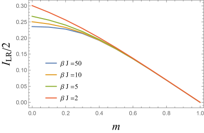
Figure 6: Renyi-2 mutual information $\mathcal{I}_{LR}^{(2)}(\Psi(m))$ between the left system and the unmeasured Majorana fermions on the right side. $m=M/N$ is the ratio of measured Majorana fermions on the right side. The mutual information is always non-vanishing for $m<1$, and vanishes only when the whole right side is measured ($m=1$).

3 Partial measurement in JT gravity

In this section, we explore the gravity dual of the SYK measurements considered above. In particular, our dual system will be Jackiw-Teitelboim (JT) gravity coupled to bulk matter, which we take to be described by $N$ copies of a CFT (capturing the $N$ Majorana fermions in the SYK model). In this and the following sections, we switch the side that is being measured; namely, we will measure the left side of the TFD. We can then calculate the mutual information in the post-measurement state between the right side and remaining fermions on the left side, this time using quantum extremal surface (QES) formula Engelhardt:2014gca . In particular, the bulk description (which relies on the location of the QES) will make manifest the entanglement wedge of the right side and thus, in turn, demonstrate how information about the center of the bulk will shift around, becoming encoded in different boundary regions as a result of measurement. Specifically, when the number of measured fermions remains small ($m\lesssim 0.26$), a significant amount of the left asymptotic region will be encoded in the remaining (unmeasured) fermions of the left system. However, as the number of measured fermions becomes large ($m\gtrsim 0.26$), the quantum extremal surface will undergo a phase transition, and information about nearly all of the left side of the bulk will become accessible from the right side. As in Antonini:2022sfm , we refer to this as teleportation of the bulk geometry, a notion which we will make more manifest in Section 4 below.

Here, we start with a more in depth description of our bulk model in Section 3.1, before moving to the holographic description of partial measurement and a computation of the mutual information in Section 3.2. Specifically, we propose for the QES prescription that the measured matter can be modeled by a boundary conformal field theory, as boundary measurements create an end-of-the-world brane in the bulk that serves as a boundary for the bulk conformal matter. Along with a comparison with the SYK results above, we find strong agreement between the QES prescription and the SYK calculation.

3.1 JT gravity with matter CFT

The action for JT gravity coupled to matter CFTs is given by

$$\begin{aligned} I=&I_{JT}(g,\phi)+I_{M}(g,\chi)\\ I_{JT}(g,\phi)=&-\frac{\phi_{0}}{16\pi G_{N}}\Big{[}\int d^{2}x\sqrt{g}R+2\int_{\partial\mathcal{M}}K\Big{]}\\ &-\frac{1}{16\pi G_{N}}\Big{[}\int d^{2}x\sqrt{g}\phi(R+2)+2\int_{\partial\mathcal{M}}\phi|_{\text{bdy}}K\Big{]},\end{aligned}$$ (47)

where $\Phi=\phi_{0}+\phi$ is a dilaton field, with $\phi$ a small fluctuation around a uniform background $\phi_{0}$. If we view this theory as coming from the dimensional reduction of a higher dimensional theory, $\phi_{0}$ would denote the area of the black hole horizon at extremality (with $\phi$ giving the area deviations for near extremal black holes), and is therefore related to ground state entropy of an extremal black hole. The first line of the JT action is a purely topological term, so that the dynamical part of the action comes solely from the second line of equation (47). We take the matter action $I_{M}(g,\chi)$ to be given by $N$ copies of a CFT with central charge $c$ (which we will take to be $c=1/2$ when comparing with the SYK results of the previous section, as each Majorana fermion can be thought of as half of a Dirac fermion).

The resulting equations of motion read

$$\begin{aligned} R&=-2,\\ T_{\mu\nu}&=\frac{1}{8\pi G_{N}}(\nabla_{\mu}\nabla_{\nu}\phi-g_{\mu\nu}\nabla^{2}\phi+g_{\mu\nu}\phi),\end{aligned}$$ (48)

where $T_{\mu\nu}$ is the stress tensor associated with the matter fields of $I_{M}$. The metric of the (Euclidean) eternal black hole is given by (see Appendix  D for a derivation)

$$ds^{2}=\frac{4\pi^{2}}{\beta^{2}}\frac{d\sigma^{2}+d\tau^{2}}{\sinh^{2}\frac{2\pi}{\beta}\sigma},$$ (49)

where $\tau$ is the imaginary time. In these coordinates, which cover one exterior portion of the two-sided black hole, the horizon is located at $\sigma\rightarrow\infty$, and the asymptotic boundary is located at $\sigma=\epsilon$. At the boundary, the induced metric satisfies the condition $g=\frac{1}{\epsilon^{2}}$, and the dilaton field satisfies $\phi(\epsilon)=\frac{\phi_{r}}{\epsilon}$. This leads to the dilaton profile,

$$\phi(\sigma)=\phi_{r}\frac{2\pi}{\beta}\frac{1}{\tanh\frac{2\pi}{\beta}\sigma}.$$ (50)

Figure 7: The doubled spacetime used to compute the bulk matter entropy. The boundary at the center of the figure is transparent. The left-most boundary and the right-most boundary are identified. $\sigma_{1}$ and $-\sigma_{2}$ denote twist operators inserted in the first and second copies of the black hole.

We will compute the entropy of a subset $R$ of the boundary system via the quantum extremal surface formula

$$S(R)=\min\{\underset{\sigma}{\text{ext}}S_{\text{gen}}(\sigma)\},$$ (51)

i.e. the smallest, extremal value of $S_{\text{gen}}$, the generalized entropy, which is given by the sum of the area of $\sigma$ (divided by $4G_{N}$) plus the bulk matter entropy in a region bound by $\sigma$. More explicitly, we compute the entropy by $S_{\text{gen}}=\frac{\Phi(\sigma)}{4G_{N}}+S_{\text{CFT}}(\sigma)$, evaluated at an extremal value of $\sigma$, which we call the quantum extremal surface. In order to do this, we need to first calculate the bulk entanglement entropy of some region extending out to the boundary. We can do this by employing a “doubling trick,” as in nezami2021quantum . The matter in the spacetime will obey reflecting boundary condition at the asypmtotic boundary $\sigma=\epsilon$. We can related the bulk entropy in this space to the entropy on a cylinder – specifically, a doubled space constructed by gluing together two copies of a black hole at their boundaries, this time with transparent boundary conditions (with a left moving mode in one copy joined to a right moving mode in the second copy). See Fig. 7 for a depiction.

In this doubled space, we can calculate the entropy of a bulk subregion (at $t=0$) by inserting twist operators at points $(\sigma_{1},0)$ in the first copy and $(-\sigma_{2},0)$ in the second copy. The entanglement entropy of the matter is then given by (see Appendix D)

$$S_{\text{double}}([-\sigma_{2},\sigma_{1}])=\frac{c}{6}\log\left[\frac{4\sinh^{2}\frac{\pi}{\beta}(\sigma_{1}+\sigma_{2})}{\sinh\frac{2\pi}{\beta}\sigma_{1}\sinh\frac{2\pi}{\beta}\sigma_{2}}\right],$$ (52)

where the subscript indicates the doubled theory. Therefore, in the original theory, a single twist operator at $(\sigma,0)$ gives an entanglement entropy

$$S_{\text{CFT}}(\sigma)=\frac{1}{2}S_{\text{double}}([-\sigma,\sigma])=\frac{c}{6}\log 2.$$ (53)

Note that from (52), the entanglement entropy does not depend on the value of $\sigma$.

If we consider the entanglement entropy of the full right system, the quantum extremal surface will be at the bifurcation surface as determined by symmetry. The generalized entropy is then given by

$$\begin{aligned} S_{\text{gen}}&=\frac{\phi_{0}}{4G_{N}}+\frac{\phi_{r}}{4G_{N}}\frac{2\pi}{\beta}+\frac{Nc}{6}\log 2,\\ &=\frac{\tilde{\phi}_{0}}{4G_{N}}+\frac{\phi_{r}}{4G_{N}}\frac{2\pi}{\beta},\end{aligned}$$ (54)

where in the first line, we have included $N$ copies of the matter CFT, and in the second line for simplicity, we have defined $\frac{\tilde{\phi}_{0}}{4G_{N}}=\frac{\phi_{0}}{4G_{N}}+\frac{Nc}{6}\log 2$. To make contact with the SYK model, we note that the first term corresponds to the ground state entropy, and the second term is a correction linear in temperature.

3.2 Measurement-induced entanglement wedge transition

With an expression for the bulk generalized entropy in hand, we can now investigate the effect of performing a measurement on one side, and in particular, calculate the mutual information between the two sides. We know that measuring the full left side will create an end-of-the-world brane in the left asymptotic region kourkoulou2017pure (and, of course, measuring nothing will leave the bulk unchanged). We thus expect that a natural bulk dual to partial measurement is the creation of an end-of-the-world brane in the bulk, but one only visible to the bulk fields dual to the measured fermions. As such, we model the bulk matter for the measured fields by a BCFT living in the bulk, with their boundary at the end-of-the-world brane. Thus, if we measure $M$ Majorana fermions on the left side, we will have $N-M$ copies of a normal matter CFT corresponding to the unmeasured fermions, and $M$ copies of a BCFT corresponding to the measured fermions, as shown in Fig. 8.

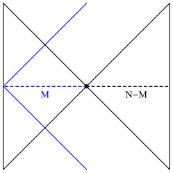
Figure 8: A boundary CFT in the $AdS_{2}$ background. The right boundary is the conventional $AdS$ boundary. Boundary conditions associated with the projective measurement of part of the left Majorana fermions are imposed at the left boundary. An ETW brane visible to $M$ bulk fermions is depicted in blue, where $M$ is the number of fermions measured in the left side.

To calculate the bulk entropy arising from the measured fermions, we insert a twist operator for the BCFT at $(\sigma,0)$, which leads to the following entanglement entropy

$$S_{\text{BCFT}}(\sigma)=\frac{c}{6}\log\left[\frac{2\sinh\frac{\pi}{\beta}(2\sigma)}{\sinh\frac{2\pi}{\beta}\sigma}\right]+\log g=\frac{c}{6}\log 2+\log g,$$ (55)

where $\log g$ is the boundary entropy of the BCFT cardy1989boundary ; affleck1991universal .

For $M\ll N$, we do not expect the position of the quantum extremal surface to change much. We can verify this by calculating the entanglement entropy of the right side,

$$\begin{aligned} S_{\text{gen}}(M)&=\frac{\phi_{0}}{4G_{N}}+\frac{\phi_{r}}{4G_{N}}\frac{2\pi}{\beta}\frac{1}{\tanh\frac{2\pi}{\beta}\sigma}+(N-M)S_{\text{CFT}}(\sigma)+MS_{\text{BCFT}}(\sigma),\\ &=\frac{\tilde{\phi}_{0}}{4G_{N}}+\frac{\phi_{r}}{4G_{N}}\frac{2\pi}{\beta}+M\log g.\end{aligned}$$ (56)

In the second line, because $S_{\text{CFT}}(\sigma)$ and $S_{\text{BCFT}}(\sigma)$ do not depend on the end point, we find $\sigma=\infty$ as the location for the quantum extremal surface, as expected.

Because $M\ll N$, there will still be a large mutual information between the right side and the unmeasured Majorana on the left after projection. Further, because the full state is pure, the entanglement entropy of the unmeasured Majorana on the left side will be equal to that of the right. As a consequence, the entanglement wedge of the left side will also extend up to the bifurcation surface. As above, we include twist operators for all copies of matter fields at the QES, including $K=N-M$ copies of a CFT, and $M$ copies of a BCFT, yielding the same entropy as in (56).

We can also consider the opposite limit, when we measure a large number of Majorana fermions, i.e., $M\sim N$ (such that the remaining number of unmeasured fermions is small $K\ll N$). To understand this limit, we invoke the bulk picture suggested in nezami2021quantum : if we have access to the remaining $K\ll N$ unmeasured boundary Majorana fermions of the left system, we expect to be able to reconstruct their dual bulk fields in a small region near the boundary. In particular, the state of the fermions remains constant on time scales $\sim 1/J$. HKLL bulk reconstruction hamilton2006holographic then implies we can reconstruct the dual fields in a small wedge near the boundary (the bulk domain of dependence of this boundary timelike region). This wedge will have size on the order of the UV cutoff $\epsilon\sim 1/J$. As a result, these fermions will have a bulk entropy associated to this UV bulk region. Since the entanglement wedge is now at the UV cutoff, we take the QES to be empty (and hence take the area contribution from the dilaton to be zero).

To compute the bulk entropy associated with the unmeasured fermions in the UV cutoff region, we note that the reduced density matrix of the unmeasured Majoranas can be found by projecting the thermal density matrix onto a fixed state. In the low temperature limit, the thermal density matrix reduces the effective available space to a low energy subsector. Therefore, the effect of measurement is constrained to that reduced low energy subspace as well. Because the SYK model is chaotic, we expect the entanglement entropy of the unmeasured fermions when $K\ll N$ will be dominated by subsystem entanglement entropy evaluated in the ground state, which is given by huang2019eigenstate

$$\frac{S_{\text{UV}}}{N}=\lambda\left(\frac{\log 2}{2}-\frac{1}{16}\arcsin\lambda^{3/2}\right),\quad\lambda=K/N.$$ (57)

where the second term originates from the nontrivial spectral density near the spectrum edge in the SYK model garcia2017analytical .

With these two limits fairly well understood, in the intermediate regime ($K\sim M$), we take the entropy to be given by $S_{\text{QES}}=\min\{S_{\text{gen}},S_{\text{UV}}\}$. While this bulk protocol may potentially seem ad hoc, we can justify the prescription by comparing it to the SYK calculations done in Section 2. As demonstrated in Fig. 9, we find a good match between the two approaches. To make this comparison, we take

$$\frac{\tilde{\phi}_{0}}{4G_{N}}=S_{0},\quad\frac{\phi_{r}}{4G_{N}}=\frac{NC}{2\pi\mathcal{J}}.$$ (58)

and $\log g=-\frac{\log 2}{12}$ . Notice that since the full state is pure, the mutual information is given by $I_{LR}=2S_{\text{QES}}$.

For $S_{0}=0.2324N$, $C=0.28$, $c=0.5$, and $\beta\mathcal{J}=50$, the phase transition in the quantum extremal surface occurs at $\lambda_{*}\approx 0.72$, see Fig. 9. Therefore, when $M>m_{*}N\approx 0.26N$ (with $m_{*}=1-\lambda_{*}$) Majorana fermions are measured in the left system, the information about the bulk that would have been encoded in those fermions becomes available to the right system, similar to Antonini:2022sfm . In other words, we find that performing a projective measurement on about a third of the left system is sufficient to allow us to teleport the information about the left side of the bulk into the right boundary, except for a small wedge at the cutoff of the left boundary. On the other hand, when a small number of fermions are measured, i.e. $M<m_{*}N\approx 0.26N$, the bulk information contained in the $M$ measured fermions is teleported into the unmeasured $K=N-M$ fermions in the same side. Therefore, the quantum extremal surface still sits at the bifurcation surface and the information about the left side of the bulk can still be accessed from the unmeasured fermions in the left side. An illustration of the entanglement wedge transition is shown in Fig. 10.

We will make efforts to better understand this transfer of bulk information by exploring quantum teleportation and traversable wormholes in the next section.

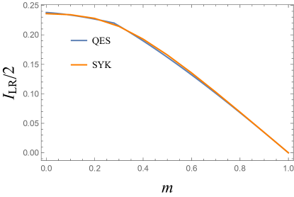
Figure 9: Comparison of the Von Neumann mutual information computed in this section using the QES prescription and the Renyi-2 mutual information compued in Section 2.3 for the SYK model. We choose the parameters $S_{0}=0.2324N$, $C=0.28$, $c=0.5$, and $\beta\mathcal{J}=50$. The two results are in good agreement. In the bulk calculation, the phase transition is sharp, while in the SYK calculation it is smoothed out.

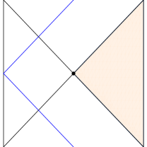
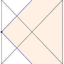
Figure 10: Measurement-induced entanglement wedge transition. The tan color denotes the entanglement wedge of the right side. (a) When a small subset of Majorana fermions is measured in the left side, i.e. $m<m_{*}$, the entanglement wedge of the right side is the right Rindler patch. (b) When a large subset of Majorana fermions is measured in the left side, i.e. $m>m_{*}$, the entanglement wedge of the right side includes part of the interior and of the left Rindler patch.

4 Quantum teleportation

As noted in the previous section, when a sufficient number of boundary fermions are measured ($m>m^{*}$), the entanglement wedge of the right boundary jumps to contain nearly the entire bulk (see Fig. 10 (b)). Consequently, almost all of the bulk (including most of the left wedge) can be reconstructed solely from the right system. To make this concrete, we can imagine releasing a particle on the left side at time $t=-t_{0}$, then measuring the left side at time $t=0$. The measurement will create an end-of-the world brane in the bulk. However, this will not effect the particle, which will continue to fall into the black hole, and in particular will not escape out to the right boundary, as illustrated in Fig. 11 (a). To extract the information from the right side, we must construct a decoding operator using information from the measurement. In the following section, we will see that by applying such a decoding operator to the right side, we will be able to extract the particle at $t=t_{0}$ in the right side. This is simply a quantum teleportation protocol, which can be used to explain the quantum information origin of the entanglement wedge transition explored above. Unsurprisingly, this boundary teleportation protocol can be related to a traversable wormhole in the bulk . In the following, we will first describe the teleportation protocol in the SYK model, which is realized as a quantum channel, and then calculate a left-right correlation function, (61), that is closely related to not only the teleportation fidelity under such a quantum channel, but also traversability in the dual picture. We will then show that the dual of this protocol provides a realization of traversable wormhole from the left side. Finally, we consider an encoding method to reach nearly perfect teleportation fidelity of an arbitrary qubit state.

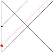
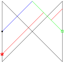
Figure 11: The red line denotes the qubit that is inserted in the left side at time $-t$. (a) Measurement is implemented at time $t=0$ in the left side, and it creates an end-of-the-world brane. The qubit cannot escaped from the horizon to the right side. (b) Measurement is implemented at time $t=0$ in the left side, in the mean time, a decoding operator according to the measurement outcome is implemented in the right side. This measurement-decoding protocol can extract the qubit out from horizon to the right side at time $t$.

4.1 Teleportation protocol

Motivated by the measurement-induced entanglement wedge phase transition studied above, we want to construct a protocol to recover the information initially stored in the left side from the right side after measurement, when the entanglement wedge extends up to the left boundary. Before describing our protocol, we should note that similar teleportation protocols have been discussed in Refs. brown2019quantum ; nezami2021quantum ; schuster2022many . Nevertheless, in the previous literature, instead of the measurement-decoding protocol normally associated with quantum teleportation, a two-sided operator is implemented in the SYK model to render the wormhole traversable. While it was argued that the two-sided coupling could be written in terms of a measurement and decoding  maldacena2017diving ; gao2021traversable ; Milekhin:2022bzx , the precise decoding protocol was not studied in detail. For instance, in the SYK model, the two-sided operator has the form of $\exp(i\theta\sum_{i}\psi_{L,i}\psi_{R,i})$, which consists of a fermionic operator in the left and right side. Thus, it is not possible to measure the fermionic operator and get an outcome.

Here, we investigate the usual measurement-decoding quantum teleportation protocol using a measurement operator of the form $i\psi_{L,2k-1}\psi_{L,2k}$ acting on the left side. Since it is a bosonic operator, we can get a measurement outcome and accordingly implement the decoding operator in the right side.

The circuit version of Fig. 11 is shown in Fig. 12. The teleportation protocol consists of three steps:

1. At time $t=-t_{0}$, an unknown state $|\psi\rangle$ is inserted in the left side;

2. At time $t=0$, a projective measurement is performed in the left side and a decoding operator is implemented in the right side according to the measurement outcome ;

3. At time $t=t_{0}$, the state $|\psi\rangle$ is teleported to the right side.

At time $t=0$, the measurement-decoding protocol should be understood as a quantum channel, which can be defined by Kraus operator,

$$K_{\textbf{l}}=(|L_{\textbf{l}}\rangle\langle L_{\textbf{l}}|)\otimes U_{\textbf{l}},$$ (59)

where $|L_{\textbf{l}}\rangle$ is the measurement outcome on the $k=1,...,N/2$ qubits, i.e.,

$$-i2\psi_{L,2k-1}\psi_{L,2k}|L_{\textbf{l}}\rangle=l_{k}|L_{\textbf{l}}\rangle,\quad k=1,...,N/2.$$ (60)

This means that the decoding operator we perform on the right side explicitly depends on the measurement outcome in the left side. Conditioned on this measurement outcome, the full protocol is shown by the circuit in Fig. 12.

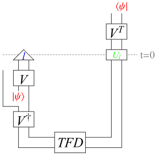
Figure 12: The circuit of the teleportation protocol. In the left side, an unknown state $|\psi\rangle$ is inserted in the past $-t_{0}$, and a measurement is applied at $t=0$. The projection is indicated by the triangle with the measurement outcome l. According to the measurement outcome, a decoding operator, denoted by $U_{\textbf{l}}$, is implemented in the right side at the same time $t=0$. After a time evolution $t_{0}$, the state $|\psi\rangle$ is teleported to the right side. $V$ denotes the time evolution operator.

To quantify the teleportation fidelity, we consider the left-right correlation function $C_{\textbf{l},Q}$ conditioned on the measurement outcome ,

$$\begin{aligned} C_{\textbf{l},Q}&=\langle TFD|Q_{R}(t_{0})\left(|L_{\textbf{l}}\rangle\langle L_{\textbf{l}}|\otimes U_{\textbf{l}}\right)Q_{L}(-t_{0})|TFD\rangle,\\ Q_{L}(-t_{0})&=(V_{L}QV^{\dagger}_{L})\otimes\mathds{1},\quad Q_{R}(t_{0})=\mathds{1}\otimes(V_{R}^{\dagger}QV_{R}),\end{aligned}$$ (61)

where $V_{L,R}$ denotes the time evolution operator in the left and right side. $Q$ is the operator being teleported. We assume the operator is properly normalized, $Q^{\dagger}Q=\mathds{1}$, so that the magnitude of the correlation function through the measurement-decoding channel (summing over all Kraus operators) is at most one.

As discussed in Section 2, in the SYK model with measurement given by (60), the Born probability does not depend on the measurement outcome. The decoding operator associated with the measurement is

$$U_{\textbf{l}}=\exp\left(-i\frac{\theta}{q}\sum_{k=1}^{N/2}il_{k}\psi_{R,2k-1}\psi_{R,2k}\right).$$ (62)

where $\theta$ is a tuning parameter. Later, we will tune $\theta$ to maximize left-right correlation. Moreover, we will see in the next subsection that the left-right correlation function does not depend on the measurement outcome. Therefore, we define the following left-right correlation function for the SYK model

$$C_{Q}=\frac{\langle TFD|Q_{R}^{\dagger}(t_{0})\left(|L_{\textbf{l}}\rangle\langle L_{\textbf{l}}|\otimes U_{\textbf{l}}\right)Q_{L}(-t_{0})|TFD\rangle}{\langle TFD|\left(|L_{\textbf{l}}\rangle\langle L_{\textbf{l}}|\otimes\mathds{1}\right)|TFD\rangle},$$ (63)

where we have omitted the subindex denoting measurement outcome because the result is independent of it. The denominator is the probability of having the measurement outcome l. Further, because the probability is independent of the outcome, we have $\langle TFD|\left(|L_{\textbf{l}}\rangle\langle L_{\textbf{l}}|\otimes\mathds{1}\right)|TFD\rangle=1/2^{N/2}$, due to the $2^{N/2}$ different outcomes. Thus, $C_{Q}=\sum_{\textbf{l}}C_{\textbf{l},Q}$, and since we have properly normalized the operator $Q$, this correlation function has maximal magnitude one. In the following, we will use large-$q$ techniques to calculate this left-right correlation function (63), and show that by properly tuning the parameter $\theta$, the fidelity can be made close to one.

4.2 Left-right correlation function in the large $q$ limit

Motivated by the left-right correlation function (63), we define the following twisted correlation function

$$\mathcal{G}_{Q}=\frac{\langle TFD|Q_{R}^{\dagger}(t_{0})\left(|L_{\textbf{l}}\rangle\langle L_{\textbf{l}}|\otimes U_{\textbf{l}}\right)Q_{L}(-t_{0})|TFD\rangle}{\langle TFD|\left(|L_{\textbf{l}}\rangle\langle L_{\textbf{l}}|\otimes U_{\textbf{l}}\right)|TFD\rangle}.$$ (64)

It is related to the left-right correlation function (63) by

$$C_{Q}=\frac{\langle TFD|\left(|L_{\textbf{l}}\rangle\langle L_{\textbf{l}}|\otimes U_{\textbf{l}}\right)|TFD\rangle}{\langle TFD|\left(|L_{\textbf{l}}\rangle\langle L_{\textbf{l}}|\otimes\mathds{1}\right)|TFD\rangle}\mathcal{G}_{Q}.$$ (65)

In this subsection, we will calculate both the twisted correlation function and the prefactor in the above relation.

In the large-$N$ limit, the basic twisted correlation function is given by $Q_{L}=\sqrt{2}\psi_{L,i}$ and $Q_{R}=-i\sqrt{2}\psi_{R,i}$, where the factor of $\sqrt{2}$ is to have a properly normalized $Q$. Teleportation of an arbitrary Majorana string, i.e. an operator consisting of an arbitrary product of SYK Majorana operators, can be obtained using the basic correlation function. In fact, the disconnected diagram built from the basic correlation function will dominate the diagrammatic expansion of correlation functions for Majorana strings in the large-$N$ limit. The basic twisted correlation function reads

$$\begin{aligned} \frac{\mathcal{G}_{\psi}}{2}&=\frac{\langle TFD|(-i\psi_{R,i}(t_{0}))\left(|L_{\textbf{l}}\rangle\langle L_{\textbf{l}}|\otimes U_{\textbf{l}}\right)\psi_{L,i}(-t_{0})|TFD\rangle}{\langle TFD|\left(|L_{\textbf{l}}\rangle\langle L_{\textbf{l}}|\otimes U_{\textbf{l}}\right)|TFD\rangle}\\ &=\frac{\langle L_{\textbf{l}}|\psi_{L,i}(-t_{0})e^{-\beta H_{L}/2}e^{-i\frac{\theta}{q}\sum_{k}il_{k}\psi_{L,2k-1}\psi_{L,2k}}\psi_{L,i}(t_{0})e^{-\beta H_{L}/2}|L_{\textbf{l}}\rangle}{\langle L_{\textbf{l}}|e^{-\beta H_{L}/2}e^{-i\frac{\theta}{q}\sum_{k}il_{k}\psi_{L,2k-1}\psi_{L,2k}}e^{-\beta H_{L}/2}|L_{\textbf{l}}\rangle},\end{aligned}$$ (66)

where we have used the properties of the thermofield double (3) to bring operators from the right side to the left side. When it is clear we will drop the subindex $L$ for simplicity. We define the following imaginary time ordered correlation function,

$$G_{\psi}(\tau_{1},\tau_{2}) = \frac{\langle L_{\textbf{l}}|e^{-\beta H}\mathcal{T}\left[e^{-i\frac{\theta}{q}\sum_{k}l_{k}i\psi_{2k-1}(\frac{\beta}{2})\psi_{2k}(\frac{\beta}{2})}\psi_{i}(\tau_{1})\psi_{i}(\tau_{2})\right]|L_{\textbf{l}}\rangle}{\langle L_{\textbf{l}}|e^{-\beta H}\mathcal{T}\left[e^{-i\frac{\theta}{q}\sum_{k}l_{k}i\psi_{2k-1}(\frac{\beta}{2})\psi_{2k}(\frac{\beta}{2})}\right]|L_{\textbf{l}}\rangle},$$ (67)

where $\mathcal{T}$ denotes imaginary time ordering, and as above $|L_{\textbf{l}}\rangle$ is the projected state with measurement outcomes given by $\textbf{l}=(l_{1},...,l_{N/2})$. Owing to the large-$N$ structure, $G_{\psi}$ does not depend on the index $i$. Note that the imaginary time correlation function and the basic twisted correlation function differ by a factor of two.

In the imaginary time contour (see Fig. 13 (a)), the measurement operator leads to boundary condition at $\tau=0$ and $\tau=\beta$ given by,

$$\psi_{2k-1}(0)=-il_{k}\psi_{2k}(0),\quad\psi_{2k-1}(\beta)=il_{k}\psi_{2k}(\beta),$$ (68)

and the decoding operator (62) leads to the following boundary condition at $\tau=\beta/2$,

$$\left(\begin{array}[]{cccc}\psi_{2k-1}(\frac{\beta^{+}}{2})\\ il_{k}\psi_{2k}(\frac{\beta^{+}}{2})\end{array}\right)=\left(\begin{array}[]{cccc}\cos\frac{\theta}{q}&-i\sin\frac{\theta}{q}\\ -i\sin\frac{\theta}{q}&\cos\frac{\theta}{q}\end{array}\right)\left(\begin{array}[]{cccc}\psi_{2k-1}(\frac{\beta^{-}}{2})\\ il_{k}\psi_{2k}(\frac{\beta^{-}}{2})\end{array}\right).$$ (75)

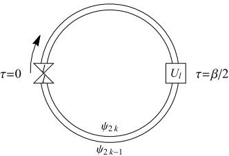
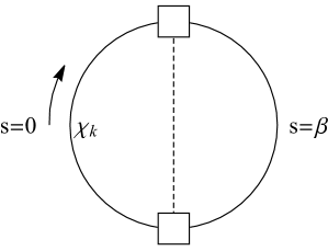
Figure 13: (a) Imaginary time contour for the twisted correlation function. In the left side ($\tau=0,\beta$), a projective measurement $|L_{\textbf{l}}\rangle\langle L_{\textbf{l}}|$ with outcome l (denoted by the two triangles) is performed, and in the right side ($\tau=\frac{\beta}{2}$), an associated decoding operator $U_{\textbf{l}}$ is applied. (b) Imaginary time contour for the Majorana field $\chi_{k}$. The boundary condition from the decoding operator becomes a rotation between $s=\frac{\beta}{2}$ and $s=\frac{3\beta}{2}$, indicated by the dashed line.

In order to take care of the boundary condition at $\tau=0,\beta$, we introduce a new field $\chi_{k}$ as in (16),

$$\chi_{k}(s)=\begin{cases}\psi_{2k-1}(s),\quad&0<s<\beta,\\ il_{k}\psi_{2k}(2\beta-s),\quad&\beta<s<2\beta,\end{cases}$$ (76)

and accordingly the bilocal field,

$$G_{\chi}(s_{1},s_{2})=\frac{2}{N}\sum_{k=1}^{N/2}\chi_{k}(s_{1})\chi_{k}(s_{2}).$$ (77)

Here, $G_{\chi}$ denotes the correlation function in the presence of the twisted boundary condition. Note that the arguments of this bilocal field $s$, run from $s=0$ to $s=2\beta$. As above, $G_{\chi}$ will satisfy the Schwinger-Dyson equation,

$$G_{\chi}=(\partial-\Sigma)^{-1},\quad\Sigma_{\chi}(s_{1},s_{2})=\frac{\mathcal{J}^{2}}{q}P(s_{1},s_{2})[2G_{\chi}(s_{1},s_{2})]^{q-1}.$$ (78)

Now, however, we will have a different boundary condition at $\tau=\beta/2$ (75). In terms the correlation function, this boundary condition becomes

$$\left(\begin{array}[]{cccc}\lim_{s_{1}/s_{2}\rightarrow\frac{\beta^{+}}{2}}G_{\chi}(s_{1},s_{2})\\ \lim_{s_{1}/s_{2}\rightarrow\frac{3\beta^{-}}{2}}G_{\chi}(s_{1},s_{2})\end{array}\right)=\left(\begin{array}[]{cccc}\cos\frac{\theta}{q}&-i\sin\frac{\theta}{q}\\ -i\sin\frac{\theta}{q}&\cos\frac{\theta}{q}\end{array}\right)\left(\begin{array}[]{cccc}\lim_{s_{1}/s_{2}\rightarrow\frac{\beta^{-}}{2}}G_{\chi}(s_{1},s_{2})\\ \lim_{s_{1}/s_{2}\rightarrow\frac{3\beta^{+}}{2}}G_{\chi}(s_{1},s_{2})\end{array}\right).$$ (85)

There are various symmetries that will further simplify the calculation (see Appendix G). In particular, the twisted correlation function satisfies various reflection conditions, which are illustrated in Fig. 14. The blue (red) dashed lines indicate (anti-)reflection conditions. Then the calculation on the full domain can be reduced to the fundamental domain, denoted by $A$, $B$, $C$, and $D$. The boundary condition (85) is illustrated by the gray lines.

In the following, we will use a large-$q$ expansion to calculate the twisted correlation function in the fundamental domain. In the large $q$ limit, and assuming $G_{\chi}(s_{1},s_{2})=G_{0}(s_{1},s_{2})\left(1+\frac{1}{q}g(s_{1},s_{2})\right)$, where $G_{0}(s_{1},s_{2})=\frac{1}{2}\text{sgn}(s_{1}-s_{2})$ is the bare propagator, we arrive at a Liouville equation similar to (35),

$$\partial_{s_{1}}\partial_{s_{2}}[G_{0}(s_{1},s_{2})g(s_{1},s_{2})]=\mathcal{J}^{2}P(s_{1},s_{2})[2G_{0}(s_{1},s_{2})]^{q-1}e^{g(s_{1},s_{2})}.$$ (86)

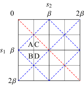
Figure 14: The full domain of twisted correlation function. The blue dashed lines indicate the reflection boundary condition, and the red dashed line indicates the anti-reflection boundary condition. With the help of these boundary conditions, we can reduce the calculation to the fundamental domains $A$, $B$, $C$ and $D$. The gray solid lines indicate the boundary condition at $s_{1,2}=\beta/2,3\beta/2$.

The remaining problem boils down to calculating the Liouville equation in the fundamental domains $A$, $B$, $C$, and $D$ with the boundary condition (85). In the large-$q$ limit, this boundary condition can be simplified (as in qi2019quantum ; gao2021traversable ), to give

$$G_{A}(s_{1},\frac{\beta}{2})\approx e^{i\frac{\theta}{q}}G_{C}(s_{1},\frac{\beta}{2}),\quad G_{B}(s_{1},\frac{\beta}{2})\approx e^{i\frac{\theta}{q}}G_{D}(s_{1},\frac{\beta}{2}).$$ (87)

Because the portions of the fundamental domain $C$ and $D$ do not cross the twist boundary condition, we assume that the solution in $C$ and $D$ has time translational symmetry qi2019quantum . On the other hand, for the fundamental domain regions $A$ and $B$, we need to solve the Liouville equation supplemented with the boundary condition (87). Via a tedious calculation, we can obtain the solution in the fundamental domains,

$$\begin{aligned} &G_{A}(s_{1},s_{2})=\hat{G}_{11}(s_{1},s_{2})\frac{e^{i\theta/q}}{\left(1+\frac{e^{i\theta}-1}{\sin\gamma}\frac{\sin(\alpha(s_{1}-\beta/2))\sin(\alpha(s_{2}-\beta/2))}{\sin(\alpha|s_{12}|+\gamma)}\right)^{2/q}},\\ &G_{B}(s_{1},s_{2})=\hat{G}_{21}(s_{1},s_{2})\frac{e^{i\theta/q}}{\left(1+\frac{e^{i\theta}-1}{\sin\gamma}\frac{\sin(\alpha\beta/2)\sin(\alpha(s_{2}-\beta/2))}{\sin(\alpha(\beta-s_{2})+\gamma)}\right)^{2/q}},\\ &G_{C}(s_{1},s_{2})=\hat{G}_{11}(s_{1},s_{2}),\quad G_{D}(s_{1},s_{2})=\hat{G}_{21}(s_{1},s_{2}),\end{aligned}$$ (88)

where $\hat{G}_{11}$ and $\hat{G}_{21}$ are given in (38) and (39), and the constant parameters are determined by (40). Solutions in other regions can be obtained by the symmetries described above.

With these results, the prefactor in (65) is now straightforward to calculate. We can start with the following equation,

$$\begin{aligned} &\frac{\partial}{\partial\theta}\log\left[\frac{\langle TFD|\left(|L_{\textbf{l}}\rangle\langle L_{\textbf{l}}|\otimes U_{\textbf{l}}\right)|TFD\rangle}{\langle TFD|\left(|L_{\textbf{l}}\rangle\langle L_{\textbf{l}}|\otimes\mathds{1}\right)|TFD\rangle}\right]\\ &=\frac{\langle L_{\textbf{l}}|e^{-\beta H}\mathcal{T}\left[\frac{1}{q}\sum_{k}l_{k}\psi_{2k-1}(\frac{\beta}{2})\psi_{2k}(\frac{\beta}{2})e^{-i\frac{\theta}{q}\sum_{k}il_{k}\psi_{2k-1}(\frac{\beta}{2})\psi_{2k}(\frac{\beta}{2})}\right]|L_{\textbf{l}}\rangle}{\langle L_{\textbf{l}}|e^{-\beta H}\mathcal{T}\left[e^{-i\frac{\theta}{q}\sum_{k}il_{k}\psi_{2k-1}(\frac{\beta}{2})\psi_{2k}(\frac{\beta}{2})}\right]|L_{\textbf{l}}\rangle}\\ &=\frac{i}{q}\frac{N}{2}G_{\chi}\left(\frac{3\beta}{2},\frac{\beta}{2}\right)=\frac{i}{q}\frac{N}{4}(\sin\gamma)^{4/q},\end{aligned}$$ (89)

which we can integrate to get

$$\frac{\langle TFD|\left(|L_{\textbf{l}}\rangle\langle L_{\textbf{l}}|\otimes U_{\textbf{l}}\right)|TFD\rangle}{\langle TFD|\left(|L_{\textbf{l}}\rangle\langle L_{\textbf{l}}|\otimes\mathds{1}\right)|TFD\rangle}=\exp\left[\frac{iN\theta}{4q}(\sin\gamma)^{4/q}\right].$$ (90)

Thus, the difference (65) between the left-right correlation function and the twisted correlation function is only a phase. Further note that this phase does not depend on the operator $Q$, and therefore the magnitude of these two correlation function is the same.

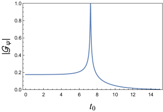
Figure 15: The magnitude of the twisted correlation function as a function of $t_{0}$. Here the parameter is chosen to be $\beta\mathcal{=}100$, $\theta=10^{-4}$ and $q=8$. The magnitude is close to one at a time $t_{0}$ that is related to the parameter $\theta$.

To get the teleportation fidelity, we take $s_{1}=\beta^{-}+it_{0}$ and $s_{2}=\frac{\beta^{-}}{2}+it_{0}$, which is in region $A$, and find

$$\mathcal{G}_{\psi}=2G_{A}\left(\beta^{-}+it_{0},\frac{\beta^{-}}{2}+it_{0}\right)\approx e^{i\theta/q}\left(\frac{\sin\gamma}{1-\frac{\theta e^{2\alpha t_{0}}}{4\sin\gamma}e^{i\gamma}}\right)^{2/q},$$ (91)

where we have expanded the equation using $e^{-\alpha t_{0}}\ll 1$, and $\theta\ll 1$. When the tuning parameter is chosen to be $\theta=4e^{-2\alpha t_{0}}\sin\gamma$, the twisted correlation reaches its maximal magnitude,

$$\mathcal{G}_{\psi}\approx\exp\left(i\frac{\pi}{q}\right)\left(\cos\frac{\gamma}{2}\right)^{2/q}.$$ (92)

In the low energy limit, $\gamma=\frac{\pi}{\beta\mathcal{J}}+\mathcal{O}\left(\frac{1}{(\beta\mathcal{J})^{2}}\right)$, the magnitude of the twisted correlation function is close to one. This means that the measurement-decoding channel can successfully teleport the Majorana operator from the left side to the right side. A plot of the magnitude of the left-right correlation function is shown in Fig. 15.

4.3 Traversable wormhole

To relate our results to a traversable wormhole, it will be simpler to start with (61). We consider the sum over measurement outcome, i.e., $\sum_{\textbf{l}}C_{\textbf{l},Q}$. The sum over measurement outcome can be rewritten as

$$\sum_{\textbf{l}}|L_{\textbf{l}}\rangle\langle L_{\textbf{l}}|\otimes U_{\textbf{l}}=\sum_{\textbf{l}}\left(\otimes_{k}|l_{k}\rangle\langle l_{k}|\right)\otimes e^{i\frac{\theta}{2q}\sum_{k}l_{k}M_{R,k}},$$ (93)

where we have introduced $M_{R,k}=-i2\psi_{R,2k-1}\psi_{R,2k}$, $M_{L,k}=-i2\psi_{L,2k-1}\psi_{L,2k}$, and $M_{L,k}|l_{k}\rangle=l_{k}|s_{k}\rangle$. Note that the projection operator is an operator-valued delta function, i.e.,

$$|l_{k}\rangle\langle l_{k}|=\delta(M_{L,k}-l_{k}).$$ (94)

Using this delta function, we arrive at a two-sided operator gao2021traversable

$$\sum_{\textbf{l}}|L_{\textbf{l}}\rangle\langle L_{\textbf{l}}|\otimes U_{\textbf{l}}=\sum_{\textbf{l}}\otimes_{k}\delta(M_{L,k}-l_{k})\otimes e^{i\frac{\theta}{2q}\sum_{k}l_{k}M_{R,k}}=e^{i\frac{\theta}{2q}\sum_{k}M_{L,k}M_{R,k}}.$$ (95)

After summing over all outcomes, the left-right correlation function is given by

$$\begin{aligned} \sum_{\textbf{l}}C_{\textbf{l},Q}&=\langle TFD|Q_{R}(t_{0})\sum_{\textbf{l}}\left(|L_{\textbf{l}}\rangle\langle L_{\textbf{l}}|\otimes U_{\textbf{l}}\right)Q_{L}(-t_{0})|TFD\rangle\\ &=\langle TFD|Q_{R}(t_{0})\left(e^{i\frac{\theta}{2q}\sum_{k}M_{L,k}M_{R,k}}\right)Q_{L}(-t_{0})|TFD\rangle.\end{aligned}$$ (96)

This is the two-sided operator that makes the wormhole traversable gao2017traversable ; maldacena2017diving ; brown2019quantum ; nezami2021quantum ; gao2021traversable .

We can compare our results with the two-sided correlation function from an $AdS_{2}$ gravity calculation. As depicted in Fig. 11, we consider the following physical setup in an $AdS_{2}$ black hole: a particle created by the operator $Q$ is released in the past $t=-t_{0}$ on the left side; at time $t_{0}=0$, a projective measurement is performed on the left side, and simultaneously, according to the measurement outcome, the decoding operator is implemented in the right side with a properly chosen tuning parameter; the particle is received in the right side at time $t=t_{0}$ with some probability. This process is effectively quantified by the two-sided correlation function maldacena2017diving

$$C_{\text{grav}}=\langle Q_{R}(t_{0})e^{i\frac{g}{N/2}\sum_{k}M_{L,k}M_{R,k}}Q_{L}(-t_{0})\rangle$$ (97)

where the expectation value is evaluated in the $AdS_{2}$ black hole state. Here, to make the comparison, we denote the two-sided deformation as $M$. In the probe limit, where the back reaction of the particle created by $Q$ on the geometry is neglected, the two-sided correlation function reads maldacena2017diving

$$C_{\text{probe}}\propto\frac{1}{\left(2-g\frac{\Delta_{M}}{2^{2\Delta_{M}+2}}G_{N}e^{\frac{2\pi}{\beta}t_{0}}\right)^{2\Delta_{Q}}}$$ (98)

where $\Delta_{M}$ and $\Delta_{Q}$ are the scaling dimension of operator $M$ and $Q$, respectively, and $G_{N}$ is Newton’s constant. It is easy to see that when $g\sim\frac{\exp[-\frac{2\pi}{\beta}t_{0}]}{G_{N}}$, the correlation function will diverge. Of course, this divergence is not physical and can be cured by smearing out the particle, but, in essence, it shows the particle traverses from the left side to the right side (see maldacena2017diving for a discussion).

Closely related to this phenomena, we find that the left-right correlation function of an arbitrary Majorana string $Q$ is given by

$$C_{Q}\propto\left(\frac{\pi/(\beta\mathcal{J})}{1-g\frac{\beta\mathcal{J}}{4\pi N}e^{2\alpha t_{0}}e^{i\gamma}}\right)^{2\Delta_{Q}},$$ (99)

where $\Delta_{Q}=p/q$, $p$ is the number of Majorana operators contained in the Majorana string $Q$, and $g=\frac{N}{4}\theta$. In the low energy limit, $\gamma\rightarrow 0$, we encounter a seemly divergent expression for the left-right correlation at $g\sim N\exp[-2\alpha t_{0}]$, which is identical to the gravity calculation with $G_{N}=1/N$. Nevertheless, it is regularized by $\gamma\approx\frac{\pi}{\beta\mathcal{J}}$ from the UV complete SYK model. This shows that the teleportation protocol realizes a traversable wormhole.

4.4 Fidelity bound

In the previous sections, we studied the teleportation of an arbitrary Majorana string $Q$, and found that our protocol yields a left-right correlation that is close to one. In this subsection, we show that the left-right correlation function gives a lower bound for state teleportation, and we construct an encoding method that can achieve a nearly perfect teleportation fidelity gao2021traversable . Note that the state teleportation fidelity is related to the fidelity of the distillation of EPR pairs yoshida2019disentangling ,

$$\langle F_{\psi}\rangle=\frac{d}{d+1}F_{EPR}+\frac{1}{d+1},$$ (100)

where $d$ is the dimension of Hilbert space of the teleported state $|\psi\rangle$, and $\langle\cdot\rangle$ implies an average over all states. Therefore, we will consider $F_{EPR}$ below. As shown in Appendix F, the distillation fidelity is lower bounded by $F_{EPR}\geq\left|\frac{1}{d^{2}}\sum_{\textbf{l},Q}C_{\textbf{l},Q}\right|^{2}$, where $C_{\textbf{l},Q}$ is given by (61), and the sum of operators $Q$ is over a complete basis for the $d$-dimensional Hilbert space. In the large-$N$ SYK model, as the left-right correlation function does not depend on the measurement outcome, the bound of the distillation fidelity simplifies to

$$F_{EPR}\geq\left|\frac{1}{d^{2}}\sum_{Q}C_{Q}\right|^{2}.$$ (101)

where $C_{Q}$ is given in (63).

Now for simplicity, we consider the teleportation of an arbitrary qubit state, for which the Hilbert space consists of two Majorana operators, $\Psi_{1},\Psi_{2}$. In order to achieve a high fidelity, we need to embed these two operators into $p$ SYK Majorana operators in the the following way,

$$\begin{aligned} &\Psi_{1}=2^{\frac{p}{2}}i^{\frac{p(p+1)}{p}}\psi^{1}\psi^{5}...\psi^{4p-3},\\ &\Psi_{2}=2^{\frac{p}{2}}i^{\frac{p(p+1)}{p}}\psi^{3}\psi^{7}...\psi^{4p-1}.\end{aligned}$$ (102)

where $p$ is an odd number and the prefactor is chosen such that these two operators satisfy $\{\Psi_{i},\Psi_{j}\}=2\delta_{ij}$, $\Psi_{i}^{\dagger}=\Psi_{i}$.

The complete basis operators for the qubit state are $\mathds{1},\Psi_{1},\Psi_{2},i\Psi_{1}\Psi_{2}$. The fidelity bound then becomes

$$F_{EPR}=\left|\frac{1}{4}\left(C_{\mathds{1}}+C_{\Psi_{1}}+C_{\Psi_{2}}+C_{i\Psi_{1}\Psi_{2}}\right)\right|^{2}=\left|\frac{1}{4}\left(1+\mathcal{G}_{\Psi_{1}}+\mathcal{G}_{\Psi_{2}}+\mathcal{G}_{i\Psi_{1}\Psi_{2}}\right)\right|^{2},$$ (103)

where in the second equality, we have used the fact that the twisted correlation function is equal to the left-right correlation function up to a constant phase. Here, we can see an interesting distinction between the teleportation of a Marjorana string such as $\Psi$ and the teleportation of an arbitrary qubit state. Apart from the requirement that the magnitude of the twisted correlation function be maximal, there is also a necessary condition that the phases of these correlation functions should align to zero modulo $2\pi$. This provides good reason to embed the qubit state into Majorana strings $\Psi_{i}$ with $p$ SYK Majorana operators.

In the large-$N$ limit, the leading contribution to the twisted correlation function is disconnected. Thus the twisted correlation function for $\Psi_{i}$ is given by the basis twisted correlation function,

$$\mathcal{G}_{\Psi_{1}}=\mathcal{G}_{\Psi_{2}}\approx i^{p}(\mathcal{G}_{\psi})^{p},\quad\mathcal{G}_{i\Psi_{1}\Psi_{2}}\approx-(\mathcal{G}_{\Psi})^{2p}.$$ (104)

We observe that though the tuning parameter $\theta$ is fixed by the time of state insertion, we still have freedom to tune $p$ to align the phase of the correlation function. In particular, from (92), the fidelity is bounded by

$$F_{EPR}=\left|\frac{1}{4}\left(1+2e^{i2\pi(\frac{p}{4}+\frac{p}{2q})}(\cos\gamma)^{2p/q}+e^{i2\pi(p+\frac{1}{2}+\frac{p}{q})}(\cos\gamma)^{4p/q}\right)\right|^{2},$$ (105)

To align the phases, we require $\frac{p}{4}+\frac{p}{2q}$ and $p+\frac{1}{2}+\frac{p}{q}$ to be close to integers. For simplicity, we consider $q\in 4\mathds{Z}$. We can then see that

$$p=\begin{cases}\frac{q}{2}+1,\quad q=4(2k+1)\\ \frac{q}{2}-1,\quad q=8k\end{cases}\quad k\in\mathds{Z},$$ (106)

which is consistent with the fact that $p$ is an odd number. In the zero temperature limit, we take $\gamma\rightarrow 0$. The fidelity bound in the large-$q$ limit is then simply given by

$$F_{EPR}\geq\left|\frac{1}{4}\left(1+2e^{i\frac{\pi}{q}}+e^{i\frac{2\pi}{q}}\right)\right|^{2}=\left(\cos\frac{\pi}{2q}\right)^{4}\approx 1-\frac{\pi^{2}}{2q^{2}}.$$ (107)

We can see that the embedding into $p$ Majorana operators can lead to a fidelity for the teleportation of an arbitrary qubit state that is close to one in the large-$q$ limit.

5 Discussion

In this work, we studied the effect of projective measurements on the thermofield double state dual to an eternal black hole; in particular, we focused on the SYK model and its dual, JT gravity coupled to matter. To characterize the post-measurement state, we calculated the Renyi-2 mutual information between the two sides of the SYK thermofield double state, which showed a transition phenomenon at low temperature. We then reproduced this mutual information calculation in the holographic JT plus matter dual. In this gravitational dual, the measurement creates an end-of-the-world brane in the bulk, and in particular, the matter fields dual to the measured fermions are then modeled by a boundary CFT. The gravitational picture makes manifest that the mutual information transition can be associated to an entanglement wedge transition, see Fig. 10. Upon measurement of a sufficiently large fraction of fermions, the entanglement wedge of the unmeasured side can jump to contain large regions behind the horizon of the black hole. On the boundary side, this change in the entanglement wedge can be understood as post-selection teleporting information about the bulk into the unmeasured boundary. We then explored this teleportation interpretation further, using the SYK model to construct an explicit protocol realizing such a teleportation. Finally, we related this telportation protocol to the physics of traversable wormholes.

In general, measurement is a nonlocal operation on a many-body quantum state, which radically changes the entanglement structure. Thus, it is not clear when a postselected state from an arbitrary measurement will give rise to a nice holographic dual (e.g. a smooth, semiclassical geometry). One exception is local projection onto a product state, which can be described by a boundary conformal field theory takayanagi2011holographic ; fujita2011aspects ; numasawa2016epr , and has been recently studied in the context of holography numasawa2016epr ; Antonini:2022sfm . Continuing in the same vein, the particular measurement operator we study is the fermion parity operator for each qubit formed by two adjacent even and odd Majorana operators (4); this is also a local projection. This measurement procedure preserves many of the nice properties of the original correlation function in the absence of measurement. Specifically, the “diagonal” correlation function remains intact after measurement, indicating the dual background $AdS_{2}$ geometry remains valid. This is consistent with the expectation that local projective measurement leaves the dual spacetime intact Antonini:2022sfm .

While a dual bulk geometry still exists, it is not left unchanged by this local projective measurement. It is now clear that these measurements create an end-of-the-world brane in bulk numasawa2016epr ; Antonini:2022sfm . Whereas the Ryu-Takayanagi formula receives only minor modifications in the presence of bulk end-of-the-world branes in the bulk, it is not well understood how the matter entropy contribution from bulk fields—a crucial contribution in e.g. black hole evaporation and the formation of islands penington2020entanglement ; penington2022replica ; Almheiri_2020 —is modified in the presence of a projection on the boundary. In a broader context, what the quantum extremal surface formula Engelhardt:2014gca is in a system with non-unitarity in the boundary—like that introduced by measurement—is an important open question. Our model above suggests that the bulk matter dual to a measured boundary can be effectively captured by a boundary CFT in two dimensional gravity. It remains to be seen whether such a proposal could be extended to more general, higher dimensional gravitational systems.

Apart from a scalar-type quantity to characterize entanglement, like the entanglement entropy, the dynamics of how information “flows” in the many-body system is often a key to understanding the physics from an information theory perspective. For instance, studying the information flow of an evaporating black hole has inspired tremendous progress in the black hole information paradox. It was proposed in Ref. Antonini:2022sfm that the information flow induced by local projective measurement on the boundary can be largely understood as information teleportation from the measured region to the unmeasured region, thanks to the (pre-measurement) entanglement resource between the two boundary subregions. Here, we have provided an explicit protocol using the UV complete SYK model to realize this expectation.

As a consequence of this information flow, an entanglement wedge transition shown in Fig. 10 naturally arises. It will be interesting to draw an analogy between this measurement-induced entanglement wedge transition and the transition between the empty set and the island in an evaporating black hole penington2020entanglement ; penington2022replica ; Almheiri_2020 . A relation of this sort may be natural in light of the Horowitz-Maldacena resolution of the black hole information problem, which invokes a post-selection at the horizon to explain how information might escape from a black hole Horowitz:2003he . In more modern language, the excess number of black hole states late in the evaporation process (in a semi-classical description) can be understood via a non-isometric map akers2022quantum ; akers2022black . Of course, projective measurements like the ones we have studied above can also give rise to non-isometries Antonini:2022sfm . We leave exploration of this potential connection to future work.

As stated above, local projection is a special kind of measurement that can preserve large portions of the dual bulk geometry. There are many unknown questions regarding “holographic measurement”. What are the neccessary properties a measurement operation should satisfy to still give rise to a dual bulk geometry? If a measurement can retain a portion of the dual spactime, what kind of geometric changes might arise from the effect of measurement (apart from the creation of an ETW brane)? An interesting extension of our results might be to to consider a soft measurement that interpolates between an identity operator and a projection. Since a dual description exists at both ends of this interpolation, namely, the pre-measurement spacetime on one end and the one including an ETW brane on the other, it seems likely that an effective geometric description exists for this soft measurement.

The attentive reader may have realized that state preparation through Euclidean time evolution can be regarded as a soft measurement of the Hamiltonian operator. An interesting question that has been recently studied in the quantum information science and many-body physics community is that of hybrid circuit evolution, where the quantum circuits consist of not only unitary operations but also non-unitary ones. In particular, when the non-unitary gates are realized as a measurement interspersing the full circuit, it also induces a transition of the entanglement structure of the final state, the so-called measurement-induced entanglement phase transition li2019measurement ; skinner2019measurement ; chan2019unitary ; jian2021measurement ; Bentsen:2021ukm . Our measurement-induced entanglement wedge transition can be viewed as the effect of “one time” measurement, in contrast to the hybrid evolution. This provides a first step in understanding the dynamical measurement-induced entanglement transition in a context with holographic duality. When the system can be effectively described by an evolution of a generic non-Hermitian Hamiltonian, several attempts have been made to explore the dual spacetime Milekhin:2022bzx ; kawabata2022dynamical ; garcia2022keldysh ; goto2022entanglement . Due to the non-Hermiticity in the boundary degrees of freedom, an analysis involving complex metrics is inevitable; nevertheless, given the larger analytical control it provides, we believe lower dimensional gravity is a promising platform to further explore the dynamical effects arising in the presence of measurements.

Appendix A One-sided measurement in the SYK model: Renyi-2 entropy

In this appendix, we derive the Schwinger-Dyson equations and the formula for the on-shell actions $I_{num}(m)$ and $I_{den}(m)$ introduced in Section 2.3. These are needed ingredients to compute the SYK Renyi-2 mutual information between the left side and the unmeasured Majorana fermions in the right side after a projective measurement on a subset of Majorana fermions is performed in the right side. We also provide some more detail about our numerical analysis.

A.1 On-shell action for the numerator of equation (42)

Let us start by computing $I_{num}(m)$. As a first step, the boundary conditions (45) suggest introducing bilocal fields analogous to the ones defined in equations (13)-(14) and the corresponding Lagrange multiplier fields $\tilde{\Sigma}_{ii}(\tau_{1},\tau_{2})$, $i=1,2,3$. The arguments now have range $\tau_{1,2}\in(0,2\beta)$. In terms of the bilocal fields, the action (2.3) takes the form

$$-I=\int d\tau_{1}d\tau_{2}\Big{[}-\frac{1}{2}\Big{(}\sum_{k=1}^{M/2}\psi_{2k-1}(\tau_{1})(\partial-\tilde{\Sigma}_{11})\psi_{2k-1}(\tau_{2})+\sum_{k=1}^{M/2}\psi_{2k}(\tau_{1})(\partial-\tilde{\Sigma}_{22})\psi_{2k}(\tau_{2})$$

$$+\sum_{j=M+1}^{N}\psi_{j}(\tau_{1})(\partial-\tilde{\Sigma}_{33})\psi_{j}(\tau_{2})\Big{)}-\frac{1}{2}\left(\frac{M}{2}\tilde{\Sigma}_{11}\tilde{G}_{11}+\frac{M}{2}\tilde{\Sigma}_{22}\tilde{G}_{22}+(N-M)\tilde{\Sigma}_{33}\tilde{G}_{33}\right)$$

$$+\frac{J^{2}}{2qN^{q-1}}\left(\frac{M}{2}\tilde{G}_{11}(\tau_{1},\tau_{2})+\frac{M}{2}\tilde{G}_{22}(\tau_{1},\tau_{2})+(N-M)\tilde{G}_{33}(\tau_{1},\tau_{2})\right)^{q}\Big{]}.$$ (108)

Similar to what we did in Section 2.1, we can now introduce a new Majorana field defined as

$$\chi_{k}(s)=\begin{cases}\psi_{2k-1}(s),&\quad 0<s<\beta/2,\\ i\psi_{2k}(\beta-s),&\quad\beta/2<s<\beta,\\ -i\psi_{2k}(2\beta-s),&\quad\beta<s<3\beta/2,\\ \psi_{2k-1}(s-\beta),&\quad 3\beta/2<s<2\beta,\\ \psi_{2k-1}(s-\beta),&\quad 2\beta<s<5\beta/2,\\ i\psi_{2k}(4\beta-s),&\quad 5\beta/2<s<3\beta,\\ -i\psi_{2k}(5\beta-s),&\quad 3\beta<s<7\beta/2,\\ \psi_{2k-1}(s-2\beta),&\quad 7\beta/2<s<4\beta.\end{cases}$$ (109)

The new Majorana satisfies the conventional anti-periodic boundary conditions for fermionic fields, i.e. $\chi_{k}(4\beta+s)=-\chi_{k}(s)$. We can then integrate out the Majorana fermions in the path integral, obtaining the following action for the path integral over the bilocal fields:

$$\begin{aligned} -\frac{I}{N}=&\frac{m}{4}\log\det(\hat{G}_{t}^{-1}-\hat{\tilde{\Sigma}})+\frac{1-m}{2}\log\det(G_{t}^{-1}-\tilde{\Sigma}_{33})\\ &-\frac{1}{2}\int d\tau_{1}d\tau_{2}\left(\frac{m}{2}\tilde{\Sigma}_{11}\tilde{G}_{11}+\frac{m}{2}\tilde{\Sigma}_{22}\tilde{G}_{22}+(1-m)\tilde{G}_{33}\right)\\ &+\frac{J^{2}}{2q}\left(\frac{m}{2}(\tilde{G}_{11}(\tau_{1},\tau_{2})+\tilde{G}_{22}(\tau_{1},\tau_{2})+(1-m)\tilde{G}_{33}(\tau_{1},\tau_{2})\right)^{q},\end{aligned}$$ (110)

where we introduced the free fermion propagator $G_{t}=\partial^{-1}$ and a compact notation for the self energy

$$\hat{\tilde{\Sigma}}(s_{1},s_{2})=\left[\begin{array}[]{cccccccc}\tilde{\Sigma}_{11}(11)&0&0&\tilde{\Sigma}_{11}(12)&\tilde{\Sigma}_{11}(13)&0&0&\tilde{\Sigma}_{11}(14)\\ 0&-\tilde{\Sigma}_{22}(11)&\tilde{\Sigma}_{22}(12)&0&0&-\tilde{\Sigma}_{22}(13)&\tilde{\Sigma}_{22}(14)&0\\ 0&\tilde{\Sigma}_{22}(21)&-\tilde{\Sigma}_{22}(22)&0&0&\tilde{\Sigma}_{22}(23)&-\tilde{\Sigma}_{22}(24)&0\\ \tilde{\Sigma}_{11}(21)&0&0&\tilde{\Sigma}_{11}(22)&\tilde{\Sigma}_{11}(23)&0&0&\tilde{\Sigma}_{11}(24)\\ \tilde{\Sigma}_{11}(31)&0&0&\tilde{\Sigma}_{11}(32)&\tilde{\Sigma}_{11}(33)&0&0&\tilde{\Sigma}_{11}(34)\\ 0&-\tilde{\Sigma}_{22}(31)&\tilde{\Sigma}_{22}(32)&0&0&-\tilde{\Sigma}_{22}(33)&\tilde{\Sigma}_{22}(34)&0\\ 0&\tilde{\Sigma}_{22}(41)&-\tilde{\Sigma}_{22}(42)&0&0&\tilde{\Sigma}_{22}(43)&-\tilde{\Sigma}_{22}(44)&0\\ \tilde{\Sigma}_{11}(41)&0&0&\tilde{\Sigma}_{11}(42)&\tilde{\Sigma}_{11}(43)&0&0&\tilde{\Sigma}_{11}(44)\end{array}\right].$$ (119)

In 119, we have used the short-hand notation $\tilde{\Sigma}_{11}(ij)=\tilde{\Sigma}_{11}\left((i-1)\beta/2+s_{1},(j-1)\beta/2+s_{2}\right)$ and $\tilde{\Sigma}_{22}(ij)=\tilde{\Sigma}_{22}\left((i-1)\beta/2-s_{1},(j-1)\beta/2-s_{2}\right)$ with $0<s_{1,2}<\beta/2$. The boundary condition resulting from the twist operator is given by

$$G_{t}(s_{1},s_{2})=\frac{1}{2}\text{sgn}(s_{1}-s_{2}),\quad s_{1,2}\in(0,2\beta),$$ (121)

$$\hat{G}_{t}(s_{1},s_{2})=\frac{1}{2}\text{sgn}(s_{1}-s_{2}),\quad s_{1,2}\in(\beta,3\beta)\text{ or }s_{1,2}(0,\beta)\cup(3\beta,4\beta).$$ (122)

and $G_{t}(s_{1},s_{2})=\hat{G}_{t}(s_{1},s_{2})=0$ otherwise.

We can now derive the Schwinger-Dyson equations by varying the action (110) for the bilocal fields:

$$\begin{aligned} &\hat{G}=(\hat{G}_{t}^{-1}-\hat{\Sigma})^{-1},\quad G=(G_{t}^{-1}-\Sigma)^{-1},\\ &\Sigma_{ii}=J^{2}\left(\frac{m}{2}(G_{11}+G_{22})+(1-m)G_{33}\right),\quad i=1,2,3.\end{aligned}$$ (123)

Here we omitted the  $\tilde{}$  to indicate that the bilocal fields are on shell. $G_{11}$ and $G_{22}$ are related to $\hat{G}$ by

$$\begin{aligned} &G_{11}(s_{1},s_{2})=\\ &\left[\begin{array}[]{cccc}\hat{G}(s_{1},s_{2})&\hat{G}(s_{1},3\beta/2+s_{2})&\hat{G}(s_{1},2\beta+s_{2})&\hat{G}(s_{1},7\beta/2+s_{2})\\ \hat{G}(3\beta/2+s_{1},s_{2})&\hat{G}(3\beta/2+s_{1},3\beta/2+s_{2})&\hat{G}(3\beta/2+s_{1},2\beta+s_{2})&\hat{G}(3\beta/2+s_{1},7\beta/2+s_{2})\\ \hat{G}(2\beta+s_{1},s_{2})&\hat{G}(2\beta+s_{1},3\beta/2+s_{2})&\hat{G}(2\beta+s_{1},2\beta+s_{2})&\hat{G}(2\beta+s_{1},7\beta/2+s_{2})\\ \hat{G}(7\beta/2+s_{1},s_{2})&\hat{G}(7\beta/2+s_{1},3\beta/2+s_{2})&\hat{G}(7\beta/2+s_{1},2\beta+s_{2})&\hat{G}(7\beta/2+s_{1},7\beta/2+s_{2})\end{array}\right],\\ &G_{22}(s_{1},s_{2})=\\ &\left[\begin{array}[]{cccc}-\hat{G}(\beta-s_{1},\beta-s_{2})&\hat{G}(\beta-s_{1},3\beta/2-s_{2})&-\hat{G}(\beta-s_{1},3\beta-s_{2})&\hat{G}(\beta-s_{1},7\beta/2-s_{2})\\ \hat{G}(3\beta/2-s_{1},\beta-s_{2})&-\hat{G}(3\beta/2-s_{1},3\beta/2-s_{2})&\hat{G}(3\beta/2-s_{1},3\beta-s_{2})&-\hat{G}(3\beta/2-s_{1},7\beta/2-s_{2})\\ -\hat{G}(3\beta-s_{1},\beta-s_{2})&\hat{G}(3\beta-s_{1},3\beta/2-s_{2})&-\hat{G}(3\beta-s_{1},3\beta-s_{2})&\hat{G}(3\beta-s_{1},7\beta/2-s_{2})\\ \hat{G}(7\beta/2-s_{1},\beta-s_{2})&-\hat{G}(7\beta/2-,3\beta/2-s_{2})&\hat{G}(7\beta/2-s_{1},3\beta+s_{2})&-\hat{G}(7\beta/2-s_{1},7\beta/2-s_{2})\end{array}\right].\end{aligned}$$ (124)

We can then discretize the imaginary time contour and numerically solve the Schwinger-Dyson equations (123) combined with equations (119) and (124) by iteration. Using the Schwinger-Dyson equations (123), the on-shell action $I_{num}(m)$ can be written as

$$-\frac{I_{num}(m)}{N} = \frac{m}{4}\left(\log\det[\hat{G}^{-1}\hat{G}_{t}]+2\log 2\right)+\frac{1-m}{2}\left(\log\det[G^{-1}G_{t}]+\log 2\right)$$ (126)

$$-\frac{J^{2}}{2}\left(1-\frac{1}{q}\right)\int d\tau_{1}d\tau_{2}\left(\frac{m}{2}(G_{11}+G_{22})+(1-m)G_{33}\right)^{q},$$

where we have used a normalization for the bare propagators

$$\log(G_{t}^{-1})-\log 2=0,\quad\log(\hat{G}_{t}^{-1})-2\log 2=0.$$ (127)

This is readily understood if we consider that $G_{t}$ is the same as a propagator for a free fermion on a contour $s\in(0,2\beta)$ and $\hat{G}_{t}$ is the same as a propagator for two free fermions on two separately contours $s\in(\beta,3\beta)$ and $s\in(0,\beta)\cup(3\beta,4\beta)$. The partition function of a free fermionic mode is simply $2$ (accounting for the occupied and unoccupied states).

Once the Schwinger-Dysons equations (123) are numerically solved, the on-shell action (126) can be evaluated. In order to minimize the error due to the discretization of the imaginary time contour, we obtain results using different finite discretizations and then extrapolate the result in the continuum limit (i.e. infinitely fine discretization). More explicitly, we divide each contour $(0,\beta)$ into $L=40,60,80,100$ segments, and then extrapolate the results in the $L\rightarrow\infty$ limit.

A.2 On-shell action for the denominator of equation (42)

In a similar fashion, the denominator of equation (42) can be written in terms of a path integral

$$\overline{(\text{Tr}[\Psi(m)])^{2}}=\int D\psi e^{-I},$$ (128)

where the action is again given by equation (2.3). We can then rewrite the action in terms of bilocal fields:

$$\begin{aligned} -\frac{I}{N}=&\frac{m}{4}\log\det(\hat{G}_{i}^{-1}-\hat{\tilde{\Sigma}})+\frac{1-m}{2}\log\det(G_{i}^{-1}-\tilde{\Sigma}_{33})\\ &-\frac{1}{2}\int d\tau_{1}d\tau_{2}\left(\frac{m}{2}\tilde{\Sigma}_{11}\tilde{G}_{11}+\frac{m}{2}\tilde{\Sigma}_{22}\tilde{G}_{22}+(1-m)\tilde{G}_{33}\right)\\ &+\frac{J^{2}}{2q}\left(\frac{m}{2}(\tilde{G}_{11}(\tau_{1},\tau_{2})+\tilde{G}_{22}(\tau_{1},\tau_{2}))+(1-m)\tilde{G}_{33}(\tau_{1},\tau_{2})\right)^{q}\end{aligned}$$ (129)

where again $G_{i}=\partial^{-1}$. The boundary conditions (46) now lead to

$$G_{i}(s_{1},s_{2})=\frac{1}{2}\text{sgn}(s_{1}-s_{2}),\quad 0<s_{1,2}<\beta\text{ or }\beta<s_{1,2}<2\beta,$$ (130)

$$\hat{G}_{i}(s_{1},s_{2})=\frac{1}{2}\text{sgn}(s_{1}-s_{2}),\quad 0<s_{1,2}<2\beta\text{ or }2\beta<s_{1,2}<4\beta.$$ (131)

and $G_{i}(s_{1},s_{2})=\hat{G}_{i}(s_{1},s_{2})=0$ otherwise. The Schwinger-Dyson equations are given by

$$\hat{G}=(\hat{G}_{i}^{-1}-\hat{\Sigma})^{-1},\quad G=(G_{i}^{-1}-\Sigma)^{-1},$$ (132)

$$\Sigma_{ii}=J^{2}\left(\frac{m}{2}(G_{11}+G_{22})+(1-m)G_{33}\right),\quad i=1,2,3.$$ (133)

with $\hat{\Sigma}$ ($\hat{G}$) given by (119) and (124). The on-shell action can then be written as

$$-\frac{I_{den}(m)}{N} = \frac{m}{4}\left(\log\det[\hat{G}^{-1}\hat{G}_{i}]+2\log 2\right)+\frac{1-m}{2}\left(\log\det[G^{-1}G_{i}]+2\log 2\right)$$ (134)

$$-\frac{J^{2}}{2}(1-\frac{1}{q})\int d\tau_{1}d\tau_{2}\left(\frac{m}{2}(G_{11}+G_{22})+(1-m)G_{33}\right)^{q},$$

where the normalization is

$$\log(G_{i}^{-1})-2\log 2=0,\quad\log(\hat{G}_{i}^{-1})-2\log 2=0.$$ (135)

We can then numerically solve the Schwinger-Dyson equations and evaluate the on-shell action $I_{den}(m)$ like we did for $I_{num}(m)$. Once we have the numerically-obtained value of both on-shell actions (126) and (134), we can finally compute the Renyi-2 entropy—given by $S_{L}^{(2)}(\Psi(m))=I_{num}(m)-I_{den}(m)$ in the saddle point approximation—and the Renyi-2 mutual information—given by $I_{LR}^{2}(\Psi(m))=2S_{L}^{(2)}(\Psi(m))$. The numerical results obtained following the procedure described in this appendix are reported in Fig. 6.

Appendix B The $m=1$ case: Kourkoulou-Maldacena state

The setup studied by Kourkoulou and Maldacena kourkoulou2017pure can be seen as a special case of our setup involving a one-sided measurement on a TFD state. In particular, when all the Majorana fermions on one side are projected using the measurement operator (4) (namely, $m=1$), the resulting post-measurement state on the other side is pure and given by a Kourkoulou-Maldacena state. For completeness, in this appendix we calculate the Renyi-2 entropy of a subset of Majorana fermions in the Kourkoulou-Maldacena state zhang2020entanglement obtained in the $m=1$ case of the analysis of Section 2 and Appendix A. Without loss of generality, we assume the Majorana fermions on the right side are projected.

We can then divide the Majorana fermions on the left side into two subsets $A=\{\psi_{i}|i=1,...,N_{A}\}$ and $A^{c}=\{\psi_{i}|i=N_{A}+1,...,N\}$ and define $\lambda=N_{A}/N$. The Renyi-2 entropy of the subset $A$ is given by

$$e^{-S_{A}^{(2)}(\lambda)}=\frac{\overline{\text{Tr}_{A}\left[\left(\text{Tr}_{\bar{A}}[\rho_{\text{KM}}]\right)^{2}\right]}}{\overline{\left(\text{Tr}[\rho_{\text{KM}}]\right)^{2}}},\quad\rho_{\text{KM}}=\text{Tr}_{R}|\Psi\rangle\langle\Psi|,$$ (136)

where $|\Psi\rangle=|\Psi(m=1)\rangle$ is defined in equation (8) and we traced over the right side (which after the measurement is in a product state with the left side). Like in our previous analysis, the numerator and denominator of equation (136) can be represented using a Euclidean path integral. The corresponding action for the numerator is the same as (2.3) on a contour $\tau\in(0,2\beta)$, but the boundary conditions are modified to take into account the insertion of a twist operator only for the first $N_{A}$ Majorana fermions on the left and the fact that all Majorana fermions are measured on the right:

$$\begin{aligned} &\psi_{i}(0)=-\psi_{i}(2\beta),\quad\psi_{i}(\beta_{-})=\psi_{i}(\beta_{+}),\quad i=1,...,N_{A},\\ &\psi_{N_{A}+j}(0)=-\psi_{N_{A}+j}(\beta_{-}),\quad\psi_{N_{A}+j}(\beta_{+})=-\psi_{N_{A}+j}(2\beta),\quad j=1,...,N-N_{A},\\ &\psi_{2k-1}(\frac{\beta_{-}}{2})=i\psi_{2k}(\frac{\beta_{-}}{2}),\quad\psi_{2k-1}(\frac{\beta_{+}}{2})=-i\psi_{2k}(\frac{\beta_{+}}{2}),\quad k=1,...,N/2,\\ &\psi_{2k-1}(\frac{3\beta_{-}}{2})=i\psi_{2k}(\frac{3\beta_{-}}{2}),\quad\psi_{2k-1}(\frac{3\beta_{+}}{2})=-i\psi_{2k}(\frac{3\beta_{+}}{2}),\quad k=1,...,N/2.\end{aligned}$$ (137)

The first line gives the anti-periodic boundary conditions for Majorana fermions in $A$ (for which a twist operator is inserted in the left); the second line gives the anti-periodic boundary conditions for Majorana fermions in $A^{c}$ (for which no twist operator is inserted); the last two lines are a consequence of the measurement of all Majorana fermions in the right side.

On the other hand, the action for the denominator is again given by equation (2.3), while the boundary conditions now reflect the fact that no twist operators are inserted in the left side:

$$\begin{aligned} &\psi_{j}(0)=-\psi_{j}(\beta_{-}),\quad\psi_{j}(\beta_{+})=-\psi_{j}(2\beta),\quad j=1,...,N,\\ &\psi_{2k-1}(\frac{\beta_{-}}{2})=i\psi_{2k}(\frac{\beta_{-}}{2}),\quad\psi_{2k-1}(\frac{\beta_{+}}{2})=-i\psi_{2k}(\frac{\beta_{+}}{2}),\quad k=1,...,N/2,\\ &\psi_{2k-1}(\frac{3\beta_{-}}{2})=i\psi_{2k}(\frac{3\beta_{-}}{2}),\quad\psi_{2k-1}(\frac{3\beta_{+}}{2})=-i\psi_{2k}(\frac{3\beta_{+}}{2}),\quad k=1,...,N/2.\end{aligned}$$ (138)

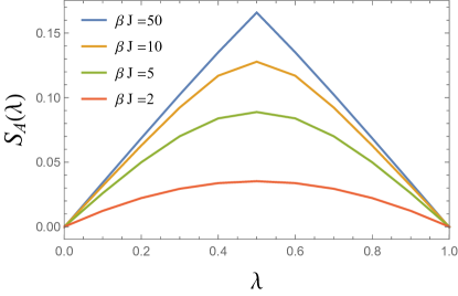
Figure 16: Renyi-2 entropy per Majorana fermion of a subset $A$ of fermions in the left side after all fermions in the right side have been measured. The left system is in the Kourkoulou-Maldacena state. $\lambda$ denotes the fraction of left fermions included in subsystem $A$. Different colors denote different values of $\beta$. The Renyi-2 entropy is symmetric around $\lambda=0.5$ due to the purity of the Kourkoulou-Maldacena state and the $O(N)$ symmetry of the large-$N$ SYK model. Increasing $\beta$ we increase the amount of Euclidean time evolution preparing the Kourkoulou-Maldacena state, and therefore the entanglement among fermions.

We can then introduce again the bilocal fields, derive and solve numerically the Schwinger-Dysons equations, evaluate the on-shell action for the numerator and denominator, and finally compute the Renyi-2 entropy in the saddle point approximation. This procedure is completely analogous to the one carried out in Section 2 and Appendix A, to which we refer for technical details. The results of our numerical evaluation of the Renyi-2 entropy as a function of the fraction $\lambda_{A}$ of fermions in subsystem $A$ are shown in Fig. 16 for different values of $\beta$.

A general feature for all curves is that the entropy increases with $\lambda$ for $\lambda<1/2$, and decreases for $\lambda>1/2$. This is a consequence of the fact that the Kourkoulou-Maldacena state—obtained in the left side by measuring all fermions in the right side—is a pure state. For this reason and due to the $O(N)$ symmetry of the SYK model at large $N$, the Renyi-2 entropy is symmetric with respect to $\lambda=1/2$. Notice also that the Renyi-2 entropy is lower for smaller values of $\beta$. This behavior can be easily understood. For $\beta=0$, the Kourkoulou-Maldacena state is simply given by the eigenstate of the measurement operator, which is a product state of the Majorana fermions (and therefore any subsystem of Majorana fermions has vanishing entropy). Increasing $\beta$, the Kourkoulou-Maldacena state is given by the same product state evolved by an amount $\beta$ of Euclidean time. Such Euclidean time evolution introduces entanglement among different Majorana fermions, increasing the Renyi-2 entropy kourkoulou2017pure ; Antonini:2021xar .

Appendix C Two-sided measurement and mutual information in the SYK model

In this appendix we consider the case where the projective measurement is performed on a subset of fermions in both sides of a SYK thermofield double. Similar to the analysis of Section 2, we measure the fermionic parity on the left and right side. The measurement operators are given by

$$\begin{aligned} &M_{R,k}=-i2\psi_{R,2k-1}\psi_{R,2k},\quad k=1,...,M/2\\ &M_{L,k}=-i2\psi_{L,2k-1}\psi_{L,2k},\quad k=(N-M)/2+1,...,N/2,\end{aligned}$$ (139)

where again we assume $M$ and $N$ are both even, and we take the large-$N$ limit with fixed $m=M/N$. The eigenvalues of the measurement operators are $r_{k},l_{k}=\pm 1$. Assume we measure the TFD state and observe the measurement outcomes $\textbf{l}=(l_{(N-M)/2+1},...,l_{N/2})$ and $\textbf{r}=(r_{1},...,r_{M/2})$ for the left side and right side, respectively. Then the post-measurement states for the measured Majorana fermions on the left and right side are given by $|L_{\textbf{l}}(m)\rangle$ and $|R_{\textbf{r}}(m)\rangle$, where

$$\begin{aligned} &M_{R,k}|R_{\textbf{r}}(m)\rangle=r_{k}|R_{\textbf{r}}(m)\rangle,\quad k=1,...,M/2,\\ &M_{L,k}|L_{\textbf{l}}(m)\rangle=l_{k}|L_{\textbf{l}}(m)\rangle,\quad k=(N-M)/2+1,...,N/2.\end{aligned}$$ (140)

The resulting full (unnormalized) post-measurement state for the two-sided system is given by

$$|\Phi_{\textbf{l,r}}(m)\rangle=\left(\mathds{1}^{(1-m)}_{R}\otimes|R_{\textbf{r}}(m)\rangle\langle R_{\textbf{r}}(m)|\right)\otimes\left(\mathds{1}^{(1-m)}_{L}\otimes|L_{\textbf{l}}(m)\rangle\langle L_{\textbf{l}}(m)|\right)|TFD\rangle,$$ (141)

where $\mathds{1}^{(1-m)}_{L,R}$ denotes the identity operator acting on the unmeasured Majorana in the left and right sides.

We are interested in computing the mutual information between the unmeasured Majorana fermions in the two sides. Because the state $|\Phi_{\textbf{l,r}}(m)\rangle$ is pure, the mutual information satisfies

$$I_{LR}(\Phi_{\textbf{l,r}}(m))=S_{L}(\Phi_{\textbf{l,r}}(m))+S_{R}(\Phi_{\textbf{l,r}}(m))-S_{LR}(\Phi_{\textbf{l,r}}(m))=2S_{L}(\Phi_{\textbf{l,r}}(m)),$$ (142)

where $\Phi_{\textbf{l,r}}(m)=|\Phi_{\textbf{l,r}}(m)\rangle\langle\Phi_{\textbf{l,r}}(m)|$ is the associated unnormalized density matrix. Like in Section 2.3, we focus on the Renyi-2 entropy

$$e^{-S_{L}^{(2)}(\Phi(m))}=\frac{\overline{\text{Tr}_{L}\left[(\text{Tr}_{R}[\Phi(m)^{2}])\right]}}{\overline{\left(\text{Tr}[\Phi(m)]\right)^{2}}}.$$ (143)

Since our analysis does not depend on the measurement outcomes, we omitted the subscripts in equation (143) and in the following calculation we set for simplicity $l_{k}=r_{k}=1$ for $k=1,...,M/2,(N-M)/2+1,...,N/2$.

(a) $1\leq i\leq M$

(b) $M<i\leq N-M$

(c) $N-M<i\leq N$

Figure 17: Imaginary time contour $\tau\in(0,2\beta)$ for the Euclidean path integral computing the numerator of equation (143) when $M<N/2$. The twist operator inserted in the left system is indicated by the dashed line. The insertion of a measurement operator in the left and right sides is indicated by the triangles. When the projective measurement operator is inserted in the left side, the effect of the twist operator is trivial and we therefore omit the dashed line. (a) Boundary conditions (146) for Majorana fermions $\psi_{i}$, $1\leq i\leq M$. (b) Boundary conditions (147) for Majorana fermions $\psi_{i}$, $M<i\leq N-M$. (c) Boundary conditions (148) for Majorana fermions $\psi_{i}$, $N-M<i\leq N$.

The path integral representation for the numerator of equation (143) is

$$\overline{\text{Tr}_{L}\left[(\text{Tr}_{R}[\Phi(m)^{2}])\right]}=\int D\psi e^{-I},$$ (144)

with the action

$$-I=-\int d\tau\sum_{j}\frac{1}{2}\psi_{j}(\tau)\partial_{\tau}\psi_{j}(\tau)+\int d\tau_{1}d\tau_{2}\frac{J^{2}}{2qN^{q-1}}\left(\sum_{j}\psi_{j}(\tau_{1})\psi_{j}(\tau_{2})\right)^{q}.$$ (145)

The imaginary time runs from $\tau=0$ to $\tau=2\beta$. We now need to specify the correct boundary conditions taking into account both the measurement operators and the insertion of a twist operator in the left side. To this end, we need to discuss two separate cases, i.e. $M<N/2$ and $M>N/2$.

 M<N/2

For $M<N/2$, the measurement on the right side is performed on Majorana fermions $\psi_{i}$ with $i\leq M$, while on the left side it is performed on Majorana fermions $\psi_{i}$ with $i>N-M$. For the Majorana fermions $\psi_{i}$ with $M<i\leq N-M$, there is no measurement in either side. A graphical representation of the boundary conditions is given in Fig. 17.

For $1\leq i\leq M$, the boundary conditions must take into account the measurement operator inserted at $\tau=\beta/2,3\beta/2$ as well as the twist operator inserted at $\tau=0,\beta,2\beta$ (see Fig. 17 (a)):

$$\begin{aligned} &k=1,...,M/2\\ &\psi_{2k-1}(\frac{\beta_{-}}{2})=i\psi_{2k}(\frac{\beta_{-}}{2}),\quad\psi_{2k-1}(\frac{\beta_{+}}{2})=-i\psi_{2k}(\frac{\beta_{+}}{2}),\\ &\psi_{2k-1}(\frac{3\beta_{-}}{2})=i\psi_{2k}(\frac{3\beta_{-}}{2}),\quad\psi_{2k-1}(\frac{3\beta_{+}}{2})=-i\psi_{2k}(\frac{3\beta_{+}}{2}),\\ &\psi_{2k-1}(0)=-\psi_{2k-1}(2\beta),\quad\psi_{2k}(0)=-\psi_{2k}(2\beta),\end{aligned}$$ (146)

where we used the shorthand notation $\beta_{\pm}$ defined in Section 2.3.

For $M<i\leq N-M$, there is no measurement operator and the twist operator is again inserted at $\tau=0,\beta,2\beta$ (see Fig. 17 (b)):

$$i=M+1,...,N-M,\quad\psi_{i}(0)=-\psi_{i}(2\beta).$$ (147)

For $N-M<i\leq N$, the boundary conditions must take into account the insertion of the measurement operator at $\tau=0,\beta,2\beta$. The twist operator at the same point is now trivial because $\langle L_{\textbf{l}}(m)|L_{\textbf{l}}(m)\rangle=1$ (see Fig. 17 (c)):

$$\begin{aligned} &k=(N-M)/2+1,...,N/2\\ &\psi_{2k-1}(0)=-i\psi_{2k}(0),\quad\psi_{2k-1}(\beta_{-})=i\psi_{2k}(\beta_{-}),\\ &\psi_{2k-1}(\beta_{+})=-i\psi_{2k}(\beta_{+}),\quad\psi_{2k-1}(2\beta)=i\psi_{2k}(2\beta).\end{aligned}$$ (148)

(a) $1\leq i\leq N-M$

(b) $N-M<i\leq M$

(c) $M<i\leq N$

Figure 18: Imaginary time contour $\tau\in(0,2\beta)$ for the Euclidean path integral computing the numerator of equation (143) when $M>N/2$. The twist operator inserted in the left system is indicated by the dashed line. The insertion of a measurement operator in the left and right sides is indicated by the triangles. When the projective measurement operator is inserted in the left side, the effect of the twist operator is trivial and we therefore omit the dashed line. (a) Boundary conditions (149) for Majorana fermions $\psi_{i}$, $1\leq i\leq N-M$. (b) Boundary conditions (150) for Majorana fermions $\psi_{i}$, $N-M<i\leq M$. (c) Boundary conditions (151) for Majorana fermions $\psi_{i}$, $M<i\leq N$.

 M>N/2

Increasing the number of measured Majorana fermions such that $M>N/2$, the measurement prescription in the right side and left side is the same as before, but now the measurement occurs in both sides for the Majorana fermions $\psi_{i}$ with $N-M<i\leq M$. A graphical representation of the resulting boundary conditions is given in Fig. 18.

For $1\leq i\leq N-M$, the boundary conditions must account for the measurement operator inserted at $\tau=\beta/2,3\beta/2$ as well as the twist operator inserted in $\tau=0,\beta,2\beta$ (see Fig. 18 (a)):

$$\begin{aligned} &k=1,...,(N-M)/2\\ &\psi_{2k-1}(\frac{\beta_{-}}{2})=i\psi_{2k}(\frac{\beta_{-}}{2}),\quad\psi_{2k-1}(\frac{\beta_{+}}{2})=-i\psi_{2k}(\frac{\beta_{+}}{2}),\\ &\psi_{2k-1}(\frac{3\beta_{-}}{2})=i\psi_{2k}(\frac{3\beta_{-}}{2}),\quad\psi_{2k-1}(\frac{3\beta_{+}}{2})=-i\psi_{2k}(\frac{3\beta_{+}}{2}),\\ &\psi_{2k-1}(0)=-\psi_{2k-1}(2\beta),\quad\psi_{2k}(0)=-\psi_{2k}(2\beta).\end{aligned}$$ (149)

For $N-M<i\leq M$, there are measurement operators inserted in both sides—namely at $\tau=0,\beta/2,\beta,3\beta/2,2\beta$—and the action of the twist operator is trivial. This leads to the boundary conditions (see Fig. 18 (b))

$$\begin{aligned} &k=(N-M)/2+1,...,M/2\\ &\psi_{2k-1}(0)=-i\psi_{2k}(0),\quad\psi_{2k-1}(\beta_{-})=i\psi_{2k}(\beta_{-}),\\ &\psi_{2k-1}(\beta_{+})=-i\psi_{2k}(\beta_{+}),\quad\psi_{2k-1}(2\beta)=i\psi_{2k}(2\beta),\\ &\psi_{2k-1}(\frac{\beta_{-}}{2})=i\psi_{2k}(\frac{\beta_{-}}{2}),\quad\psi_{2k-1}(\frac{\beta_{+}}{2})=-i\psi_{2k}(\frac{\beta_{+}}{2}),\\ &\psi_{2k-1}(\frac{3\beta_{-}}{2})=i\psi_{2k}(\frac{3\beta_{-}}{2}),\quad\psi_{2k-1}(\frac{3\beta_{+}}{2})=-i\psi_{2k}(\frac{3\beta_{+}}{2}).\end{aligned}$$ (150)

Finally, for $M<i\leq N$, the boundary conditions must take into account the measurement operator inserted at $\tau=0,\beta,2\beta$, while the twist operator at the same point is trivial (see Fig. 18 (c)):

$$\begin{aligned} &k=M/2+1,...,N/2\\ &\psi_{2k-1}(0)=-i\psi_{2k}(0),\quad\psi_{2k-1}(\beta_{-})=i\psi_{2k}(\beta_{-}),\\ &\psi_{2k-1}(\beta_{+})=-i\psi_{2k}(\beta_{+}),\quad\psi_{2k-1}(2\beta)=i\psi_{2k}(2\beta).\end{aligned}$$ (151)

The denominator of equation (143) can also represented by a path integral with the same action (145). The difference is in the boundary conditions, because there is no twist operator. More explicitly, the boundary conditions for the denominator are given by equations (146)-(151) after replacing the last line in equation (146), equation (147), and the last line in equation (149) by

$$\psi_{i}(0)=-\psi_{i}(\beta_{-}),\quad\psi_{i}(\beta_{+})=-\psi_{i}(2\beta),\quad i=1,...,N-M.$$ (152)

Having identifying the boundary conditions, we can now proceed to introduce bilocal fields, derive and numerically solve the Schwinger-Dyson equations, evaluate the numerator and denominator on-shell actions $I_{num}(m)$ and $I_{den}(m)$, and finally compute the Renyi-2 mutual information—which is given in the saddle point approximation by $I_{LR}^{(2)}(\Phi(m))=2(I_{num}(m)-I_{den}(m))$. This analysis is completely analogous to the one carried out for the one-sided measurement in Section 2.3 and Appendix A, and we will therefore omit it here.

Our numerical results for the Renyi-2 mutual information $\mathcal{I}^{(2)}_{LR}(\Phi(m))=I_{LR}^{(2)}(\Phi(m))/N$ are shown in Fig. 19. As in the one-sided measurement case, the mutual information remains finite for any $m<1$ and only vanishes for $m=1$. In other words, the left and right systems are completely disentangled only when all Majorana fermions are measured. One way to understand this result is to remember that at infinite temperature the TFD state reduces to EPR pairs between the left and right Majorana fermions. In this case the mutual information is

$$\mathcal{I}^{\Phi}_{LR}(m)=\begin{cases}(1-2m)\log 2,&m<1/2,\\ 0,&m\geq 1/2.\end{cases}$$ (153)

The transition between the entangled phase and the completely disentangled phase occurs at $m=1/2$. This can be readily understood if we recall that for $m=1/2$ (which is $M=N/2$) one fermion is measured for each one of the $N$ EPR pairs. In particular, the right fermion of each EPR pair is measured for $i=1,...,N/2$, while the left fermion of each EPR pair is measured for $i=N/2+1,...,N$. Now imagine we turn on a small imaginary time evolution, i.e. we consider the TFD state at high but finite temperature. Then the all-to-all interaction in the Hamiltonian will generate entanglement between the two sides even for $m>1/2$. This is particularly evident for example in the $\beta\mathcal{J}=2$ numerical result in Fig. 19.

Finally, we would like to remark that the holographic dual analysis of the two-sided measurement setup described in the present Appendix is complicated by the fact that when large subsets of fermions are measured on both sides, it is not clear whether a geometric bulk dual description still exists. Therefore, when $m$ is small we expect the bulk dual analysis to remain substantially similar to the one described in Section 3 for the one-sided measurement case. But when $m$ is large, it is not clear what bulk geometry is left behind by the measurement, if any. For intermediate values of $m$, the transition from a semiclassical geometry to a non-geometric description could be radical and it is not well-understood. We thus leave the bulk dual analysis of the two-sided measurement case for future work.

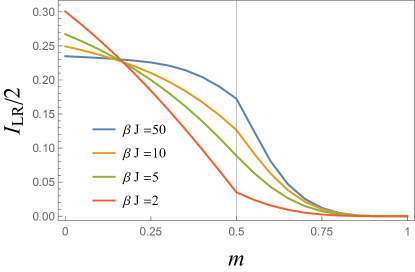
Figure 19: Renyi-2 mutual information $\mathcal{I}_{LR}^{(2)}(\Phi(m))$ between unmeasured Majorana fermions on the left and right sides for the two-sided measurement case. $m=M/N$ is the ratio of measured Majorana fermions on the left and right sides. The mutual information is always non-vanishing for $m<1$, and vanishes only when all the Majorana fermions are measured ($m=1$).

Appendix D Entanglement entropy in JT gravity with matter CFT

Varying the dilaton and metric in the JT plus matter action (equation  (47)), respectively, yield the equations of motion

$$R=-2,$$ (154)

$$\frac{1}{8\pi G_{N}}(\nabla_{\mu}\nabla_{\nu}\phi-g_{\mu\nu}\nabla^{2}\phi+g_{\mu\nu}\phi)=T_{\mu\nu},$$ (155)

where $T_{\mu\nu}$ is the stress tensor of the matter CFT. We first consider the solution at zero temperature, setting $T_{\mu\nu}$ to zero. The metric in Euclidean Poincaré coordinates is

$$ds^{2}=\frac{dt^{2}+dz^{2}}{z^{2}},$$ (156)

and we implement the following boundary conditions at $z=\epsilon$ maldacena2016conformal ,

$$g|_{\text{bdy}}=\frac{1}{\epsilon^{2}},\quad\phi(\epsilon)=\frac{1}{\epsilon}.$$ (157)

The solution for the dilaton is then given by

$$\phi=\frac{\alpha+\gamma t+\delta(t^{2}+z^{2})}{z},$$ (158)

where $\alpha,\gamma,\delta$ are constants determined by the boundary conditions, $\alpha=1$, $\gamma=\delta=0$.

To describe a thermal state with temperature $1/\beta$, we can make a series of coordinate transformations. To this end, we first introduce $x=z+it$, $\bar{x}=z-it$ with $ds^{2}=\frac{4dxd\bar{x}}{(x+\bar{x})^{2}}$. Now then take

$$x=\frac{\beta}{2\pi}\tanh\frac{\pi}{\beta}y,\quad\bar{x}=\frac{\beta}{2\pi}\tanh\frac{\pi}{\beta}\bar{y}.$$ (159)

Finally, with $y=\sigma+i\tau$, $\bar{y}=\sigma-i\tau$, the metric becomes

$$ds^{2}=\frac{4\pi^{2}}{\beta^{2}}\frac{d\sigma^{2}+d\tau^{2}}{\sinh^{2}\frac{2\pi}{\beta}\sigma}.$$ (160)

Implementing the boundary condition at $\sigma=\epsilon$, $g_{\tau\tau}=\frac{1}{\epsilon^{2}}$, $\phi(\epsilon)=\frac{\phi_{r}}{\epsilon}$, yields the dilaton solution

$$\phi(\sigma)=\phi_{r}\frac{2\pi}{\beta}\frac{1}{\tanh\frac{2\pi}{\beta}\sigma}.$$ (161)

Figure 20: Two copies of Poincare disk with one of them filling outside $|z|>1$.

We can now turn to understanding the bulk matter entropy, computed via a “doubling trick.” We introduce a second Euclidean copy of the spacetime, glued together as in Fig. 20. To this end, we employ a (final) coordinate transformation,

$$\begin{aligned} &\text{first copy}\\ &z=e^{\frac{2\pi}{\beta}(\sigma+i\tau)},\quad\bar{z}=e^{\frac{2\pi}{\beta}(\sigma-i\tau)},\quad ds^{2}=\frac{4dzd\bar{z}}{(1-|z|^{2})^{2}},\quad|z|<1,\\ &\text{second copy}\\ &z=e^{-\frac{2\pi}{\beta}(\sigma+i\tau)},\quad\bar{z}=e^{-\frac{2\pi}{\beta}(\sigma-i\tau)},\quad ds^{2}=\frac{4dzd\bar{z}}{(1-|z|^{2})^{2}},\quad|z|>1.\end{aligned}$$ (162)

The metric is identical in the two copies, except one copy is mapped to $|z|<1$, and the other one to $|z|>1$. In other words, the two copies are related by the transformation $z\rightarrow\frac{1}{z}$. The free Dirac fermion can propagate in the entire plane, as shown in Fig. 20. Note that the UV cutoff of the two copies is located at $|z|=1\pm\frac{2\pi\epsilon}{\beta}$, respectively.

Since the metric differs from a flat space by only a Weyl factor $ds^{2}=\frac{\sum_{i}dx^{i}dx^{i}}{\Omega(x)^{2}}$—and as noted above, the fermions propagate in the entire plane—we know the entanglement entropy between two twist operators at $\bf x_{1},x_{2}$ near the vacuum state is given by

$$S_{\text{CFT}}({\bf x}_{1},{\bf x}_{2})=\frac{c}{6}\log\frac{{\bf x_{12}^{2}}}{\Omega({\bf x_{1}})\Omega({\bf x_{2}})},$$ (163)

where ${\bf x}_{12}={\bf x}_{1}-{\bf x}_{2}$. Finally, the dilaton field in this coordinate is given by

$$\phi(z,\bar{z})=\phi_{r}\frac{2\pi}{\beta}\frac{1+|z|^{2}}{|1-|z|^{2}|}.$$ (164)

Appendix E Haar random unitary model for TFDs with measurement

In this appendix, we construct a simple model that shows the essential physics of measurement-induced entanglement wedge phase transitions in the context of bulk reconstruction. Our simple model consists of two random unitaries $U_{L}$ and $U_{R}$ with equal dimension $2^{N}$, drawn from a Haar distribution. To allow for a more general setup, we take the bulk state of the system to be $|\psi\rangle$. As shown in Fig. 21, these random unitaries map the state $|\psi\rangle$ from bulk to boundary (we take the incoming legs at the bottom of each unitary to be the bulk Hilbert space, and the outgoing legs on top of each unitary to be the boundary Hilbert space, which we refer to as the left and right sides for simplicity).

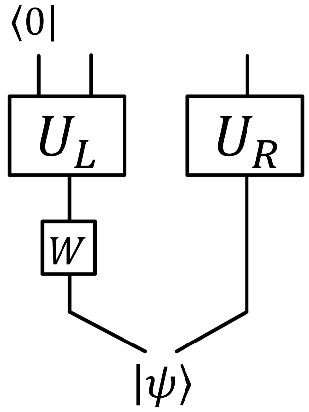
Figure 21: A model with two random unitaries, $U_{L}$ and $U_{R}$, representing the two sides each with $N$ qubits. $|\psi\rangle$ denotes a bulk state. $M$ out of $N$ qubits in the left side are projected to state $|0\rangle$. $W$ denotes an operator acting on the left bulk Hilbert space.

In analogy with the measurements considered in the main text, we measure $M$ qubits in the left boundary Hilbert space. In the main text, we found a phase transition occurs when the fraction $m=M/N$ of measured fermions exceeds a critical value $m^{*}$ (see e.g. Fig. 1). When $m>m^{*}$, the information that was stored in the left side before measurement is teleported to the right side. Here, in this simple model, we ask a similar question. Suppose we have an operator $W$ in the left bulk Hilbert space acting on the state $|\psi\rangle$. How many qubits $M$ need to be measured in the left side such that this operator can be successfully reconstructed in the right boundary Hilbert space? In Fig. 21, $M$ out of $N$ qubits in the left side are projected to state $|0\rangle$. The measurement outcome is not important here since we are interested in the typical behavior of random unitaries drawn from a Haar distribution.

To answer this question, we employ the technique introduced in Ref. akers2022black ; Antonini:2022sfm to give a bound on the reconstruction error. This calculation is straightforward, and we refer to Ref. Antonini:2022sfm for details. Here we just present the final result. Let $W_{R}$ be an operator acting on the right boundary Hilbert space, and $V=\frac{1}{2^{M/2}}U_{L}\otimes U_{R}$ be the linear map from the bulk to the boundary for both sides (here the prefactor comes from measurements). The reconstruction error is defined by

$$||VW|\psi\rangle-W_{R}V|\psi\rangle||\leq\epsilon_{1},$$ (165)

where $||.||$ denotes the norm of the state. The reconstruction error for a typical error modeled by a random unitary drawn from the Haar distribution is bounded by $\epsilon_{1}\leq\sqrt{\epsilon_{2}}$, where

$$\epsilon_{2}\leq 2\sqrt{\frac{2^{N-M}}{e^{S^{(2)}_{L}(\Psi)}}}.$$ (166)

$S^{(2)}_{L}(\Psi)=\text{Tr}_{R}\left[\text{Tr}_{L}(\Psi)^{2}\right]$ is the pre-measurement Renyi-2 entanglement entropy between left and right side evaluated for the state $\Psi=|\psi\rangle\langle\psi|$. This bound intuitively states that the reconstruction would be successful if the measurement is implemented on a subset of fermions large enough that the entanglement of the remaining $N-M$ unmeasured qubits is much smaller than the pre-measurement entanglement between the two sides, i.e. the entanglement resource. With this understanding, we can give an estimate of the critical value of $m$ by solving $\frac{2^{N-M}}{e^{S^{(2)}_{L}(\Psi)}}=1$. The transition point is then given by

$$m^{*}=1-\frac{S^{(2)}_{L}(\Psi)}{N\log 2}.$$ (167)

Roughly speaking, this means that the critical point is determined by the pre-measurement entanglement between the two sides: the greater the entanglement, the fewer number of qubits needs to be measured to achieve the transition.

Appendix F Bound on teleportation fidelity

In this appendix, we are going to relate the bound on teleportation fidelity to the left-right correlation functions studied in Section 4. Our discussion is similar to that of Ref. schuster2022many . We will use diagrams to represent states and amplitudes. Assuming two copies of the same Hilbert space, each consisting of $N/2$ qubits, we define some relevant states and projection operators as follows,

$$\begin{aligned} {\begin{array}[]{c}\vbox{\vskip 1.19998pt\hbox{\hskip 0.79999pt\includegraphics[scale={0.4}]{Figures/fig_TFD_1.png}}}\end{array}}&=\frac{1}{(\text{Tr}[e^{-\beta H}])^{1/2}}\sum_{n=1}^{N/2}e^{-\beta E_{n}}|E_{n}\rangle\otimes|E_{n}\rangle,\\ {\begin{array}[]{c}\vbox{\vskip 1.19998pt\hbox{\hskip 0.79999pt\includegraphics[scale={0.4}]{Figures/fig_EPR.png}}}\end{array}}&=\frac{1}{d^{1/2}}\sum_{i=1}^{d}|i\rangle\otimes|i\rangle,\\ {\begin{array}[]{c}\vbox{\vskip 1.05002pt\hbox{\hskip 0.70001pt\includegraphics[scale={0.35}]{Figures/fig_projection.png}}}\end{array}}&=\bigotimes_{k=1}^{N/2}|s_{k}\rangle\langle s_{k}|,\end{aligned}$$ (168)

where $H$ denotes the Hamiltonian and $|E_{n}\rangle$ denotes the energy eigenstates. $|s_{k}\rangle,s_{k}=\pm$ are two possible states of a qubit, and $|s_{k}\rangle\langle s_{k}|$ denotes a projection operator. In this appendix, we use $s_{k}$ to denote the measurement outcome (note the change in notation from Section 4, where we used $l_{k}$ to denote the measurement outcome).

The state teleportation protocol conditioned on measurement outcome $s_{k}$ is given by

$${\begin{array}[]{c}\vbox{\vskip 1.19998pt\hbox{\hskip 0.79999pt\includegraphics[scale={0.4}]{Figures/fig_teleport.png}}}\end{array}}$$ (170)

where $U$ is a time evolution operator and $U_{s}$ is a unitary operator dependent on the measurement outcome, which we refer to as a decoding operator. $D$ is another decoding operator at the end of the teleportation. Thus, the teleportation protocol consists of three parts:

1. At time $t=-t_{0}$, a state $|\psi\rangle$ is inserted in the left side;

2. At time $t=0$, a projective measurement is performed in the left side and a decoding operator is implemented in the right side according to the measurement outcome;

3. At time $t=t_{0}$, another decoding operator $D$ is performed in the right side, and the state is teleported to the right side.

At time $t=0$, the measurement-decoding protocol should be understood as a quantum channel, which can be defined by a Kraus operator,

$$K_{\textbf{s}}=\left(\otimes_{k}|s_{k}\rangle\langle s_{k}|\right)\otimes U_{\textbf{s}},\quad\sum_{\textbf{s}}K_{\textbf{s}}^{\dagger}K_{\textbf{s}}=1,$$ (171)

where the decoding operator we perform on the right side depends on the measurement outcome on the left. Conditioned on the measurement outcome, the full protocol is given in (170).

The state teleportation fidelity is related to the fidelity of the distillation of EPR pairs yoshida2019disentangling ,

$${\begin{array}[]{c}\vbox{\vskip 1.10999pt\hbox{\hskip 0.73999pt\includegraphics[scale={0.37}]{Figures/fig_distill.png}}}\end{array}}$$ (173)

Here, instead of inserting a state, a swap between two qubits is performed in the right side, and finally a distillation of EPR states between the swap qubit is implemented. The average fidelity of state teleportation is related to the fidelity of EPR distillation by,

$$\langle F_{\psi}\rangle=\frac{d}{d+1}F_{EPR}+\frac{1}{d+1},$$ (174)

where $d$ is the dimension of the state Hilbert space, and $\langle\cdot\rangle$ implies an average over all states.

The fidelity for distillation of an EPR state is

$$F_{EPR}=\sum_{\textbf{s}_{1},\textbf{s}_{2}}{\begin{array}[]{c}\vbox{\vskip 1.80002pt\hbox{\hskip 1.20001pt\includegraphics[scale={0.6}]{Figures/fig_F_EPR.png}}}\end{array}}=\frac{1}{d^{4}}\sum_{\textbf{s}_{1},\textbf{s}_{2}}\sum_{Q_{1},Q_{2}}{\begin{array}[]{c}\vbox{\vskip 1.80002pt\hbox{\hskip 1.20001pt\includegraphics[scale={0.6}]{Figures/fig_F_EPR_operator.png}}}\end{array}}$$ (177)

where in the first diagram, the projection operator enforces $\textbf{s}_{1}=\textbf{s}_{2}$. The sum over all possible measurement outcomes occurs because the full fidelity is given by the sum of fidelities conditioned on each measurement outcome. To get the second diagram, the swap operator is replaced by the following identity,

$${\begin{array}[]{c}\vbox{\vskip 1.5pt\hbox{\hskip 1.0pt\includegraphics[scale={0.5}]{Figures/fig_swap.png}}}\end{array}}=\frac{1}{d}\sum_{Q}{\begin{array}[]{c}\vbox{\vskip 1.5pt\hbox{\hskip 1.0pt\includegraphics[scale={0.5}]{Figures/fig_swap_operator.png}}}\end{array}}$$ (180)

where $Q$ is a basis operator living in the $d$ dimensional Hilbert space. For instance for $d=2$, $Q=\mathds{1},X,Y,Z$ the identity and three Pauli matrices. Then we move one of the operators to the right side, and define $\tilde{Q}=D^{\dagger}QD$. In the case of a qubit, the decoding operator is $D=Y$ brown2019quantum ; nezami2021quantum ; schuster2022many . For the SYK model we consider in the main text, the decoding operator is trivial $D=\mathds{1}$, and so we neglect it in the main text.

Thus, the distillation fidelity is lower bounded by

$$F_{EPR}=\frac{1}{d^{4}}\sum_{\textbf{s}_{1},\textbf{s}_{2}}\sum_{Q_{1},Q_{2}}{\begin{array}[]{c}\vbox{\vskip 1.85999pt\hbox{\hskip 1.23999pt\includegraphics[scale={0.62}]{Figures/fig_F_EPR_operator.png}}}\end{array}}\geq\frac{1}{d^{4}}\sum_{\textbf{s}_{1},\textbf{s}_{2}}\sum_{Q_{1},Q_{2}}{\begin{array}[]{c}\vbox{\vskip 1.80002pt\hbox{\hskip 1.20001pt\includegraphics[scale={0.6}]{Figures/fig_F_bound.png}}}\end{array}}.$$ (183)

Namely,

$$F_{EPR}\geq\left|\sum_{\textbf{s},Q}\frac{1}{d^{2}}C_{\textbf{s},Q}\right|^{2},$$ (184)

where the left-right correlation function $C_{\textbf{s},Q}$ is given by

$$\begin{aligned} &C_{\textbf{s},Q}=\langle TFD|\tilde{Q}_{R}^{\dagger}(t_{0})\left[\left(\otimes_{k}|s_{k}\rangle\langle s_{k}|\right)\otimes U_{\textbf{s}}\right]Q_{L}(-t_{0})|TFD\rangle,\\ &Q_{L}(-t_{0})=(U_{L}QU^{\dagger}_{L})\otimes\mathds{1},\quad\tilde{Q}_{R}(t_{0})=\mathds{1}\otimes(U_{R}^{\dagger}\tilde{Q}U_{R}),\end{aligned}$$ (185)

where $U_{L,R}$ denotes the time evolution operator in the left and right side. Thus, the left-right correlation function is closely related to the fidelity bound.

Appendix G Symmetries of the twisted correlation function

In this appendix, we discuss the symmetries of the twisted correlation function, which are used to simplify the calculations in the main text by reducing to a fundamental domain. Recall the twisted correlation function is defined as

$$G_{\chi}(s_{1},s_{2})=$$ (186)

$$\frac{\langle L_{\textbf{l}}|e^{-\beta H}\mathcal{T}\left[O(\frac{\beta}{2})\left(\begin{array}[]{cccc}\psi_{2k-1}(s_{1})\psi_{2k-1}(s_{2})&il_{k}\psi_{2k-1}(s_{1})\psi_{2k}(2\beta-s_{2})\\ il_{k}\psi_{2k}(2\beta-s_{1})\psi_{2k-1}(s_{2})&-\psi_{2k}(2\beta-s_{1})\psi_{2k}(2\beta-s_{2})\end{array}\right)\right]|L_{\textbf{l}}\rangle}{\langle L_{\textbf{l}}|e^{-\beta H}\mathcal{T}\left[O(\frac{\beta}{2})\right]|L_{\textbf{l}}\rangle}$$ (189)

where $\psi(\tau)=e^{H\tau}\psi e^{-H\tau}$ is the imaginary time evolution, and $O(\frac{\beta}{2})=e^{-i\frac{\theta}{q}\sum_{k}l_{k}i\psi_{2k-1}(\frac{\beta}{2})\psi_{2k}(\frac{\beta}{2})}$ is the decoding operator. Because the Majorana field $\chi_{k}$ satisfies conventional anti-periodic boundary conditions, we have

$$G_{\chi}(s_{1},s_{2})=-G_{\chi}(s_{2},s_{1}),\quad G_{\chi}(s_{1},s_{2})=-G_{\chi}(2\beta+s_{1},s_{2}).$$ (190)

The twisted correlation function is real if $\theta$ is a purely imaginary number, $G_{\chi}(s_{1},s_{2})=G_{\chi}(s_{1},s_{2})^{*}$. This is because we can find a real representation for all operators, including $O(\frac{\beta}{2})$. Thus, we take $\theta$ imaginary, then analytically continue it to a real number. If we take the complex conjugate of the twisted correlation function, we get

$$\begin{aligned} &G_{\chi}(s_{1},s_{2})^{*}\\ &=\frac{\langle L_{\textbf{l}}|\mathcal{T}\left[O(-\frac{\beta}{2})\left(\begin{array}[]{cccc}\psi_{2k-1}(-s_{2})\psi_{2k-1}(-s_{1})&-il_{k}\psi_{2k}(-2\beta+s_{2})\psi_{2k-1}(-s_{1})\\ -il_{k}\psi_{2k-1}(-s_{2})\psi_{2k}(-2\beta+s_{1})&-\psi_{2k}(-2\beta+s_{2})\psi_{2k}(-2\beta+s_{1})\end{array}\right)\right]e^{-\beta H}|L_{\textbf{l}}\rangle}{\langle L_{\textbf{l}}|\mathcal{T}\left[O(-\frac{\beta}{2})\right]e^{-\beta H}|L_{\textbf{l}}\rangle}\\ &=\frac{\langle L_{\textbf{l}}|e^{-\beta H}\mathcal{T}\left[O(\frac{\beta}{2})\left(\begin{array}[]{cccc}\psi_{2k-1}(\beta-s_{2})\psi_{2k-1}(\beta-s_{1})&-il_{k}\psi_{2k}(-\beta+s_{2})\psi_{2k-1}(\beta-s_{1})\\ -il_{k}\psi_{2k-1}(\beta-s_{2})\psi_{2k}(-\beta+s_{1})&-\psi_{2k}(-\beta+s_{2})\psi_{2k}(-\beta+s_{1})\end{array}\right)\right]|L_{\textbf{l}}\rangle}{\langle L_{\textbf{l}}|e^{-\beta H}\mathcal{T}\left[O(\frac{\beta}{2})\right]|L_{\textbf{l}}\rangle}\\ &=G_{\chi}(\beta-s_{2},\beta-s_{1}),\end{aligned}$$ (191)

where we have used $[\psi(\tau)]^{\dagger}=\psi(-\tau)$ to get the first line. In the second line, we bring the operator $e^{-\beta H}$ from the right to the left by shifting the time by $\beta$ for all operators. The last line can be obtained by recalling the definition of $\chi_{k}$ and its anti-periodic boundary conditions.

Moreover, the twisted correlation function is invariant under $\psi_{2k-1}\rightarrow\psi_{2k}$, $\psi_{2k}\rightarrow-\psi_{2k-1}$. The large-$N$ action is invariant under $O(N)$ transformations, so it is invariant under this subgroup. Now we should check the measurement-decoding channel under this transformation. Both the projected state $|L_{\textbf{l}}\rangle$ and the decoding operator $O(\frac{\beta}{2})$ are invariant because $-2i\psi_{2k-1}\psi_{2k}$ is invariant. Therefore, the twisted correlation function is invariant, which leads to the following properties

$$G_{\chi}(s_{1},s_{2})=-G_{\chi}(2\beta-s_{1},2\beta-s_{2})=G_{\chi}(2\beta-s_{2},2\beta-s_{1}).$$ (192)

In summary, (190), (191), and (192) lead to the following (anti-)reflection conditions

$$\begin{aligned} &\text{anti-reflection about}\quad s_{1}-s_{2}=0:\quad G_{\chi}(s_{1},s_{2})=-G_{\chi}(s_{2},s_{1}),\\ &\text{reflection about}\quad s_{1}-s_{2}=\beta:\quad G_{\chi}(s_{1},s_{2})=G_{\chi}(s_{2},s_{1}-\beta),\\ &\text{reflection about}\quad s_{1}-s_{2}=-\beta:\quad G_{\chi}(s_{1},s_{2})=G_{\chi}(s_{2}-\beta,s_{1}+\beta),\\ &\text{reflection about}\quad s_{1}+s_{2}=2\beta:\quad G_{\chi}(s_{1},s_{2})=G_{\chi}(2\beta-s_{2},2\beta-s_{1}),\\ &\text{reflection about}\quad s_{1}+s_{2}=2\beta:\quad G_{\chi}(s_{1},s_{2})=G_{\chi}(\beta-s_{2},\beta-s_{1}),\\ &\text{reflection about}\quad s_{1}+s_{2}=\frac{3}{2}\beta:\quad G_{\chi}(s_{1},s_{2})=G_{\chi}(\frac{3}{2}\beta-s_{2},\frac{3}{2}\beta-s_{1}).\end{aligned}$$ (193)

They are illustrated in Fig. 14. With the help of these symmetries, we can reduce the calculation from the full domain to the fundamental domain $A$, $B$, $C$ and $D$, as discussed in the main text.

References

- (1) J. M. Maldacena, The Large N limit of superconformal field theories and supergravity, Adv. Theor. Math. Phys. 2 (1998) 231–252, [hep-th/9711200].
- (2) E. Witten, Anti-de Sitter space and holography, Adv. Theor. Math. Phys. 2 (1998) 253–291, [hep-th/9802150].
- (3) S. S. Gubser, I. R. Klebanov and A. M. Polyakov, Gauge theory correlators from noncritical string theory, Phys. Lett. B 428 (1998) 105–114, [hep-th/9802109].
- (4) O. Aharony, S. S. Gubser, J. M. Maldacena, H. Ooguri and Y. Oz, Large N field theories, string theory and gravity, Phys. Rept. 323 (2000) 183–386, [hep-th/9905111].
- (5) S. Ryu and T. Takayanagi, Aspects of Holographic Entanglement Entropy, JHEP 08 (2006) 045, [hep-th/0605073].
- (6) S. Ryu and T. Takayanagi, Holographic derivation of entanglement entropy from the anti–de sitter space/conformal field theory correspondence, Physical review letters 96 (2006) 181602.
- (7) V. E. Hubeny, M. Rangamani and T. Takayanagi, A Covariant holographic entanglement entropy proposal, JHEP 07 (2007) 062, [0705.0016].
- (8) B. Swingle, Entanglement Renormalization and Holography, Phys. Rev. D 86 (2012) 065007, [0905.1317].
- (9) M. Van Raamsdonk, Building up spacetime with quantum entanglement, Gen. Rel. Grav. 42 (2010) 2323–2329, [1005.3035].
- (10) J. Maldacena and L. Susskind, Cool horizons for entangled black holes, Fortsch. Phys. 61 (2013) 781–811, [1306.0533].
- (11) N. Engelhardt and A. C. Wall, Quantum Extremal Surfaces: Holographic Entanglement Entropy beyond the Classical Regime, JHEP 01 (2015) 073, [1408.3203].
- (12) X. Dong, D. Harlow and A. C. Wall, Reconstruction of Bulk Operators within the Entanglement Wedge in Gauge-Gravity Duality, Phys. Rev. Lett. 117 (2016) 021601, [1601.05416].
- (13) D. Harlow, The Ryu–Takayanagi Formula from Quantum Error Correction, Commun. Math. Phys. 354 (2017) 865–912, [1607.03901].
- (14) S. Antonini, G. Bentsen, C. Cao, J. Harper, S.-K. Jian and B. Swingle, Holographic measurement and bulk teleportation, 2209.12903.
- (15) T. Numasawa, N. Shiba, T. Takayanagi and K. Watanabe, Epr pairs, local projections and quantum teleportation in holography, Journal of High Energy Physics 2016 (2016) 1–52.
- (16) S. Sachdev and J. Ye, Gapless spin fluid ground state in a random, quantum heisenberg magnet, Phys. Rev. Lett. 70 (1993) 3339, [cond-mat/9212030].
- (17) A. Kitaev, “A simple model of quantum holography.” http://online.kitp.ucsb.edu/online/entangled15/, Feb. 12, April 7, and May 27, 2015.
- (18) J. Maldacena and D. Stanford, Remarks on the sachdev-ye-kitaev model, Physical Review D 94 (2016) 106002.
- (19) J. Maldacena, D. Stanford and Z. Yang, Conformal symmetry and its breaking in two-dimensional nearly anti-de sitter space, Progress of Theoretical and Experimental Physics 2016 (2016) .
- (20) J. Maldacena, Eternal black holes in anti-de sitter, Journal of High Energy Physics 2003 (2003) 021.
- (21) J. Maldacena and X.-L. Qi, Eternal traversable wormhole, 1804.00491.
- (22) V. P. Su, Variational preparation of the thermofield double state of the Sachdev-Ye-Kitaev model, Phys. Rev. A 104 (2021) 012427, [2009.04488].
- (23) C. Teitelboim, Gravitation and Hamiltonian Structure in Two Space-Time Dimensions, Phys. Lett. B 126 (1983) 41–45.
- (24) R. Jackiw, Lower Dimensional Gravity, Nucl. Phys. B 252 (1985) 343–356.
- (25) I. Kourkoulou and J. Maldacena, Pure states in the syk model and nearly- gravity, arXiv preprint arXiv:1707.02325 (2017) .
- (26) S. Antonini and B. Swingle, Holographic boundary states and dimensionally reduced braneworld spacetimes, Phys. Rev. D 104 (2021) 046023, [2105.02912].
- (27) J. L. Cardy, Boundary conditions, fusion rules and the verlinde formula, Nuclear Physics B 324 (1989) 581–596.
- (28) S. Nezami, H. W. Lin, A. R. Brown, H. Gharibyan, S. Leichenauer, G. Salton et al., Quantum Gravity in the Lab: Teleportation by Size and Traversable Wormholes, Part II, 2102.01064.
- (29) V. Chandrasekaran and A. Levine, Quantum error correction in syk and bulk emergence, arXiv preprint arXiv:2203.05058 (2022) .
- (30) S. Antonini, B. Grado-White, S.-K. Jian and B. Swingle, Quantum extremal surface formula in the syk model, In preparation .
- (31) P. Gao, D. L. Jafferis and A. C. Wall, Traversable wormholes via a double trace deformation, Journal of High Energy Physics 2017 (2017) 1–25.
- (32) J. Maldacena, D. Stanford and Z. Yang, Diving into traversable wormholes, Fortschritte der Physik 65 (2017) 1700034.
- (33) A. R. Brown, H. Gharibyan, S. Leichenauer, H. W. Lin, S. Nezami, G. Salton et al., Quantum gravity in the lab: teleportation by size and traversable wormholes, arXiv preprint arXiv:1911.06314 (2019) .
- (34) P. Gao and D. L. Jafferis, A traversable wormhole teleportation protocol in the syk model, Journal of High Energy Physics 2021 (2021) 1–44.
- (35) P. Zhang, Entanglement entropy and its quench dynamics for pure states of the sachdev-ye-kitaev model, Journal of High Energy Physics 2020 (2020) 1–20.
- (36) S. Sachdev, Bekenstein-Hawking Entropy and Strange Metals, Phys. Rev. X 5 (2015) 041025, [1506.05111].
- (37) C. Liu, X. Chen and L. Balents, Quantum entanglement of the sachdev-ye-kitaev models, Physical Review B 97 (2018) 245126.
- (38) P. Zhang, C. Liu and X. Chen, Subsystem rényi entropy of thermal ensembles for syk-like models, SciPost Physics 8 (2020) 094.
- (39) I. Affleck and A. W. Ludwig, Universal noninteger “ground-state degeneracy”in critical quantum systems, Physical Review Letters 67 (1991) 161.
- (40) A. Hamilton, D. Kabat, G. Lifschytz and D. A. Lowe, Holographic representation of local bulk operators, Physical Review D 74 (2006) 066009.
- (41) Y. Huang, Y. Gu et al., Eigenstate entanglement in the sachdev-ye-kitaev model, Physical Review D 100 (2019) 041901.
- (42) A. M. García-García and J. J. Verbaarschot, Analytical spectral density of the sachdev-ye-kitaev model at finite n, Physical Review D 96 (2017) 066012.
- (43) T. Schuster, B. Kobrin, P. Gao, I. Cong, E. T. Khabiboulline, N. M. Linke et al., Many-body quantum teleportation via operator spreading in the traversable wormhole protocol, Physical Review X 12 (2022) 031013.
- (44) A. Milekhin and F. K. Popov, Measurement-induced phase transition in teleportation and wormholes, 2210.03083.
- (45) X.-L. Qi and A. Streicher, Quantum epidemiology: operator growth, thermal effects, and syk, Journal of High Energy Physics 2019 (2019) 1–28.
- (46) B. Yoshida and N. Y. Yao, Disentangling scrambling and decoherence via quantum teleportation, Physical Review X 9 (2019) 011006.
- (47) M. Miyaji, S. Ryu, T. Takayanagi and X. Wen, Boundary states as holographic duals of trivial spacetimes, Journal of High Energy Physics 2015 (May, 2015) 152, [1412.6226].
- (48) T. Takayanagi, Holographic dual of a boundary conformal field theory, Physical review letters 107 (2011) 101602.
- (49) M. Fujita, T. Takayanagi and E. Tonni, Aspects of ads/bcft, Journal of High Energy Physics 2011 (2011) 1–40.
- (50) G. Penington, Entanglement wedge reconstruction and the information paradox, Journal of High Energy Physics 2020 (2020) 1–84.
- (51) G. Penington, S. H. Shenker, D. Stanford and Z. Yang, Replica wormholes and the black hole interior, Journal of High Energy Physics 2022 (2022) 1–87.
- (52) A. Almheiri, T. Hartman, J. Maldacena, E. Shaghoulian and A. Tajdini, Replica wormholes and the entropy of hawking radiation, Journal of High Energy Physics 2020 (may, 2020) .
- (53) G. T. Horowitz and J. M. Maldacena, The Black hole final state, JHEP 02 (2004) 008, [hep-th/0310281].
- (54) C. Akers and G. Penington, Quantum minimal surfaces from quantum error correction, SciPost Physics 12 (2022) 157.
- (55) C. Akers, N. Engelhardt, D. Harlow, G. Penington and S. Vardhan, The black hole interior from non-isometric codes and complexity, arXiv preprint arXiv:2207.06536 (2022) .
- (56) Y. Li, X. Chen and M. P. Fisher, Measurement-driven entanglement transition in hybrid quantum circuits, Physical Review B 100 (2019) 134306.
- (57) B. Skinner, J. Ruhman and A. Nahum, Measurement-induced phase transitions in the dynamics of entanglement, Physical Review X 9 (2019) 031009.
- (58) A. Chan, R. M. Nandkishore, M. Pretko and G. Smith, Unitary-projective entanglement dynamics, Physical Review B 99 (2019) 224307.
- (59) S.-K. Jian, C. Liu, X. Chen, B. Swingle and P. Zhang, Measurement-induced phase transition in the monitored sachdev-ye-kitaev model, Phys. Rev. Lett. 127 (Sep, 2021) 140601.
- (60) G. S. Bentsen, S. Sahu and B. Swingle, Measurement-induced purification in large-N hybrid Brownian circuits, Phys. Rev. B 104 (2021) 094304, [2104.07688].
- (61) K. Kawabata, A. Kulkarni, J. Li, T. Numasawa and S. Ryu, Dynamical quantum phase transitions in syk lindbladians, arXiv preprint arXiv:2210.04093 (2022) .
- (62) A. M. García-García, L. Sá, J. J. Verbaarschot and J. P. Zheng, Keldysh wormholes and anomalous relaxation in the dissipative sachdev-ye-kitaev model, arXiv preprint arXiv:2210.01695 (2022) .
- (63) K. Goto, M. Nozaki, K. Tamaoka and M. T. Tan, Entanglement dynamics of the non-unitary holographic channel, arXiv preprint arXiv:2211.03944 (2022) .