A BayeSN Distance Ladder: $H_{0}$ from a consistent modelling of Type Ia supernovae from the optical to the near infrared

Abstract

The local distance ladder estimate of the Hubble constant ($H_{0}$) is important in cosmology, given the recent tension with the early universe inference. We estimate $H_{0}$ from the Type Ia supernova (SN Ia) distance ladder, inferring SN Ia distances with the hierarchical Bayesian SED model, BayeSN. This method has a notable advantage of being able to continuously model the optical and near-infrared (NIR) SN Ia light curves simultaneously. We use two independent distance indicators, Cepheids or the tip of the red giant branch (TRGB), to calibrate a Hubble-flow sample of 67 SNe Ia with optical and NIR data. We estimate $H_{0}=74.82\pm 0.97$ (stat) $\pm\,0.84$ (sys) km ${\rm s}^{-1}\,{\rm Mpc}^{-1}$ when using the calibration with Cepheid distances to 37 host galaxies of 41 SNe Ia, and $70.92\pm 1.14$ (stat) $\pm\,1.49$ (sys) km ${\rm s}^{-1}\,{\rm Mpc}^{-1}$ when using the calibration with TRGB distances to 15 host galaxies of 18 SNe Ia. For both methods, we find a low intrinsic scatter $\sigma_{\rm int}\lesssim 0.1$ mag. We test various selection criteria and do not find significant shifts in the estimate of $H_{0}$. Simultaneous modelling of the optical and NIR yields up to $\sim$15% reduction in $H_{0}$ uncertainty compared to the equivalent optical-only cases. With improvements expected in other rungs of the distance ladder, leveraging joint optical-NIR SN Ia data can be critical to reducing the $H_{0}$ error budget.

1 Introduction

The Hubble constant ($H_{0}$) describes the present-day expansion rate and sets the absolute distance scale of the universe. The recent measurement of $H_{0}$ from the local SN Ia distance ladder, calibrated to Cepheid variables (e.g. Riess et al., 2022) is in tension with the inference from the early universe inference using the cosmic microwave background (Planck Collaboration, 2020). Such a tension could potentially be a signature of non-standard physics beyond the standard cosmological model and several studies have reviewed the merits of exotic cosmological models to resolve this discrepancy (Knox & Millea, 2020; Shah et al., 2021; Schöneberg et al., 2022). The local measurements are based on a calibration of the absolute luminosity of Type Ia supernovae (SNe Ia) using independent distances to host galaxies of nearby SNe Ia. This is termed as the “cosmic distance ladder". This claimed tension suggests that the universe at present is expanding about 8-10$\%$ faster than predicted assuming the $\Lambda$CDM model, the concordance cosmological scenario. Currently, there are internal differences in the local distance ladder estimate of $H_{0}$. Calibrating the SN Ia luminosity using the tip of the red giant branch (TRGB) method (e.g. Freedman, 2021) does not show a significant tension with the early universe inference. Understanding differences in the individual rungs of the distance ladder is important to understand whether the tension is a sign of novel cosmological physics or unresolved sources of systematic error.

In this paper, we focus on the SN Ia rung of the distance ladder. We implement a new methodology for determining the distances to SNe Ia and, using them to infer $H_{0}$. Conventionally SN Ia distances have been derived from optical lightcurves, and subsequent cross-checks have been performed in the near infrared (e.g., see Dhawan et al., 2018; Burns et al., 2018). More recently, Galbany et al. (2022), have performed a near-infrared-only analysis with the most updated Cepheid calibrator sample, finding consistent results with the estimates in Riess et al. (2022). They apply a Gaussian process regression method to only single filter NIR ($J$ or $H$ band) photometry to obtain SN Ia apparent magnitudes from only a single waveband. Here, we test the impact of using a data-driven statistical model for SN Ia spectral-energy distributions, BayeSN (Thorp et al., 2021; Mandel et al., 2022), to improve the inference of the SN Ia distances. Crucially, BayeSN models a continuous SED from the optical through to the NIR and simultaneously fits the optical and NIR lightcurves. It utilises all available information for each SN Ia in a wide wavelength range. The BayeSN model has been previously applied to study dust properties of SNe Ia in context of their host galaxies (Thorp et al., 2021; Thorp & Mandel, 2022) and for analysing supernova siblings to estimate $H_{0}$ from multiple SNe Ia in the same galaxy (Ward et al., 2022). The BayeSN spectral energy distribution (SED) model has been constructed simultaneously from the optical to the NIR wavelengths ($\sim 0.35-1.8\,\mu$m). In the NIR wavebands, SNe Ia have been shown to have a small intrinsic scatter (e.g. see Elias et al., 1981, 1985; Meikle, 2000; Krisciunas et al., 2004, for earlier works on the uniform behaviour of SNe Ia in the NIR). NIR magnitudes at maximum light exhibit small scatter without the typical lightcurve shape and colour corrections that are applied in the optical wavelengths (e.g. Wood-Vasey et al., 2008; Mandel et al., 2009; Folatelli et al., 2010; Mandel et al., 2011; Barone-Nugent et al., 2012; Kattner et al., 2012; Weyant et al., 2014; Friedman et al., 2015; Avelino et al., 2019; Johansson et al., 2021). Simultaneously fitting the optical and NIR lightcurves also enables a more accurate determination of the host galaxy dust extinction (e.g. Krisciunas et al., 2000, 2007; Mandel et al., 2011; Burns et al., 2014; Thorp & Mandel, 2022). The BayeSN model can be used to exploit both the low luminosity dispersion of SNe Ia in the NIR, and improve upon constraints by leveraging the long wavelength baseline of SN Ia observations. With optical and NIR data, BayeSN has been demonstrated to have lower root-mean-square (RMS) scatter than conventional lightcurve fitting tools, e.g. SNooPy (Burns et al., 2011), SALT2 (Guy et al., 2007). Given the unique capabilities of BayeSN to simultaneously model the optical and NIR to infer more accurate distances, we investigate the impact of the improved distance inference model on cosmological parameter estimation. In this study, we focus on $H_{0}$ from the local distance ladder.

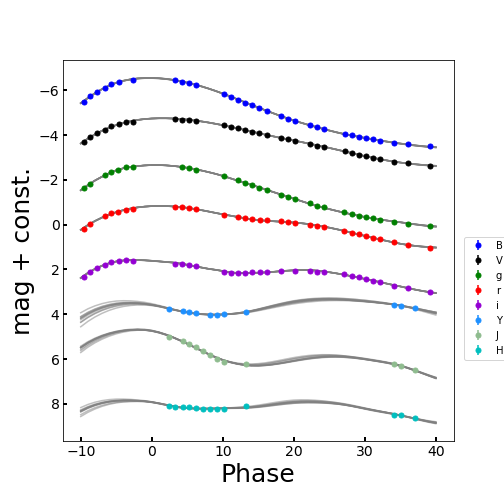
Figure 1: An example BayeSN fit to the multi-wavelength optical-NIR data for SN 2015F (Cartier et al., 2014). BayeSN simultaneously fits all the data from the $B$ to the $H$ band for this object, exploiting the constraining power of the NIR.

In addition to current datasets, there are several forthcoming surveys with a large component dedicated to NIR observations, e.g. the Carnegie Supernova Project-II (CSP-II; Phillips et al., 2019), SIRAH (Jha et al., 2019) with HST, FLOWS (Müller-Bravo et al., 2022), and the DEHVILS survey using UKIRT (Konchady et al., 2022). Moreover, recent studies of high-$z$ ($0.2<z<0.6$) SN Ia observed in the NIR via the RAISIN program have demonstrated the promise of using the NIR as an independent route to measure dark energy properties (Jones et al., 2022). Future space missions, e.g. the Roman Space Telescope, with optimised sensitivity in the NIR wavebands are forecast to precisely constrain properties of accelerated expansion (Hounsell et al., 2018; Rose et al., 2021). In this paper, we focus on the constraints on $H_{0}$ from a low-$z$ sample. We describe our dataset and methodology in Section 2 and present our results in Section 3. We discuss the results in context of other studies in the literature and conclude in section 4.

Table 1: Calibrator sample used for inferring $H_{0}$ with independent distances to the host galaxy derived from Cepheid variables. The SN distance and uncertainty are reported along with the inferred lightcurve shape parameter $\theta$ and the absorption in the $V$-band, $A_{V}$. We also report the logarithm of the host stellar mass and whether the sample is in the NIR at max subsample (see text for details). The table is truncated for formatting reasons, entire table is available online.

SN	Host	$\mu_{\rm SN}$	$\sigma_{\rm SN,fit}$	$\mu_{\rm Ceph}$	$\sigma_{\rm Ceph}$	$\theta$	$A_{V}$	log10 Host mass	NIR at max	Photometry Reference
1981B	NGC 4536	30.893	0.054	30.838	0.051	0.076	0.253	9.69	N	[1,2]
1990N	NGC 4639	31.803	0.058	31.818	0.085	-0.701	0.168	9.80	N	[3]
1994ae	NGC 3370	32.019	0.059	32.123	0.052	-0.426	0.308	10.20	N	[4]
1995al	NGC 3021	32.234	0.062	32.475	0.160	-0.956	0.356	10.30	N	[5]
1997bp	NGC 4680	32.524	0.052	32.606	0.208	0.213	0.479	9.75	N	[6]

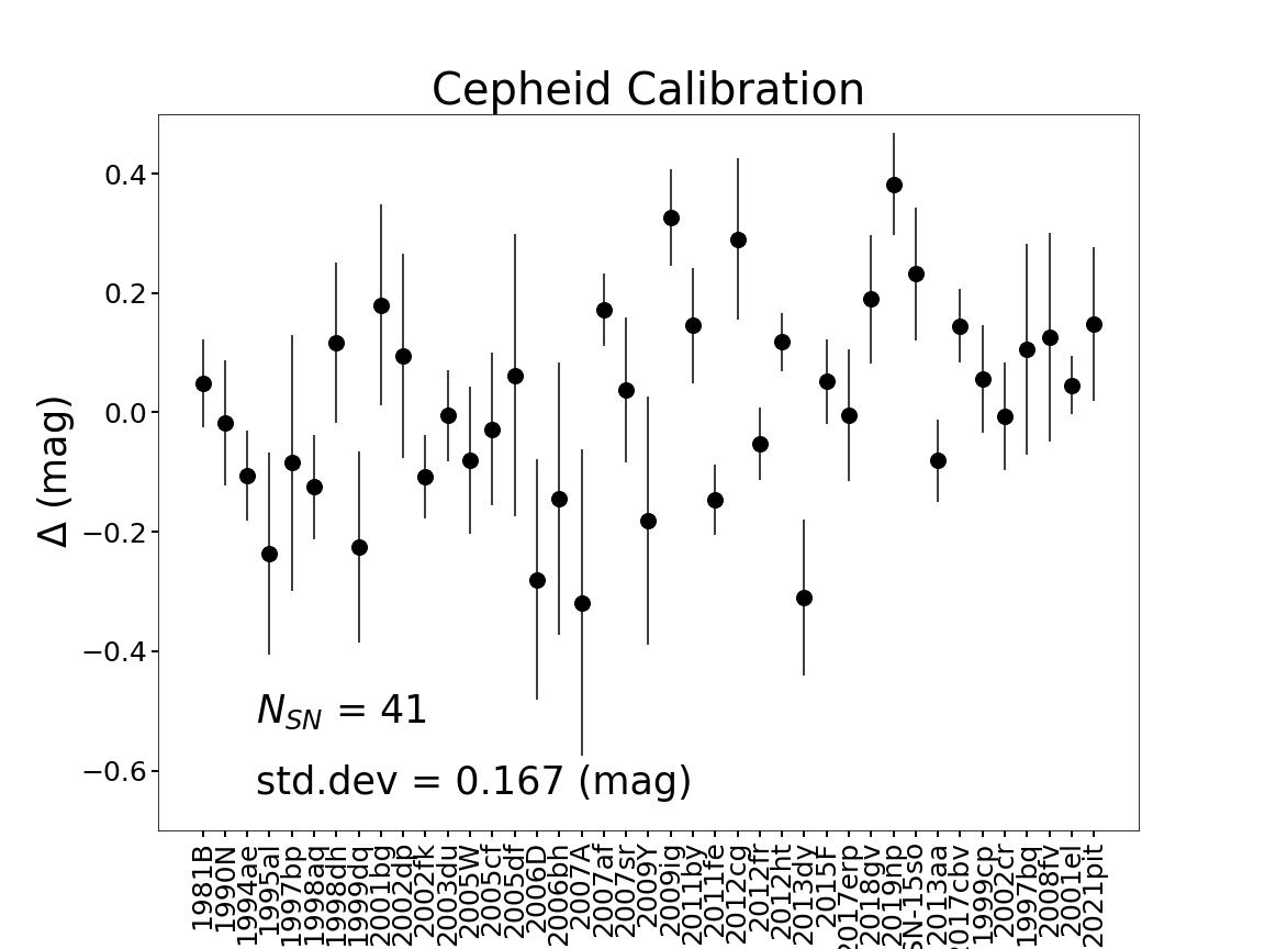
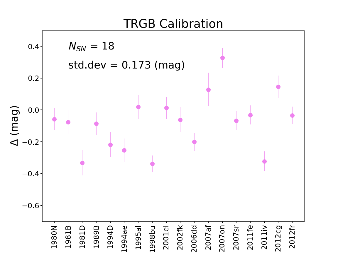
Figure 2: Difference, $\Delta=\hat{\mu}_{\text{SN}}-\hat{\mu}_{\text{Cal}}$, between the SN Ia photometric distance and the independent distance to the host galaxy for the calibrator sample, using the Cepheid (left, black) and TRGB calibration of the distance (right, violet) to the SN Ia host galaxies. The sample standard deviation of these differences is indicated. We note that the plotted errors do not include the SN intrinsic scatter, however, the intrinsic scatter was added in quadrature in the analysis. We note that, in each case, the average of the differences corresponds to the differences between the reference scale assumed in BayeSN and the scale set by the independent distance indicator. We also emphasize that this does not impact our final estimate of $H_{0}$.

2 Data and Methodology

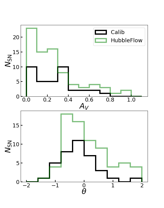
Figure 3: (Left): Comparison of the $A_{V}$ (top) and $\theta$ (bottom) distribution between the Cepheid calibrator (green) and the Hubble flow samples (red). We note that the calibrator sample has fewer SNe with high $A_{V}$ and $\theta$ and test the impact of this mismatch on the final $H_{0}$ (see text for details)

Figure 4: Same as figure 3 but for the TRGB calibration

For constraining $H_{0}$ using SNe Ia modelled with BayeSN, we need a sample of nearby SNe Ia with independent distances to their host galaxies (calibrators). The most widely used methods to get distances to nearby galaxies are Cepheid variables (Riess et al., 2022) and the tip of the red giant branch (TRGB) method (Freedman, 2021), both of which have been used for $H_{0}$ inference with sample of order tens of SN Ia galaxies. Secondly, we require a sample of SNe Ia in the Hubble flow ($z>0.01$).

For our Cepheid-calibrated sample we use the host galaxy distances from Riess et al. (2022), for a total of 37 host galaxies of 41 SNe Ia. Out of these 41 SNe Ia, 15 have NIR data ($\geq 1\,\mu$m). Individual sources for the datasets are detailed in Table 1. For the 23 new SNe Ia in the sample of calibrators presented in Riess et al. (2022), we take the data provided as part of the Pantheon+ data release (Brout et al., 2021; Scolnic et al., 2021). For the TRGB method, we use the sample of 18 galaxies with distances provided Freedman et al. (2019). A summary of the samples is provided in Table 1 and 2 for the Cepheid and TRGB method, respectively. While the current number of SNe Ia with NIR data is significantly lower than those with optical data, there have been a few dedicated follow-up programs, e.g. the Carnegie Supernova Project (CSP-I; Krisciunas et al., 2017), the Center for Astrophysics (CfA) SN program (Wood-Vasey et al., 2008; Friedman et al., 2015) as well as programs for follow-up of the Palomar Transient Factory (PTF; Barone-Nugent et al., 2012), intermediate Palomar Transient Factory (iPTF; Johansson et al., 2021) and the SweetSpot survey (Weyant et al., 2018). Since our aim is to model the optical and NIR simultaneously we take the training sample of SNe Ia from Mandel et al. (2022) with $z\geq 0.01$, a total of 67 SNe, as our fiducial Hubble flow sample. This sample was compiled from the CSP-I and CfA samples and objects from the literature (c.f. Table 1 of Mandel et al. 2022). We obtain the heliocentric frame redshifts from Avelino et al. (2019).

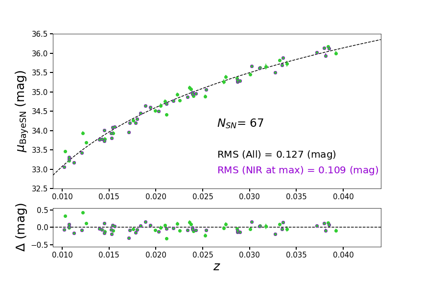
Figure 5: Photometric BayeSN optical+NIR distance estimates versus redshifts for the Hubble flow sample in our analysis. The error bars do not include the $\sigma_{\rm int}$ term.

We fit the lightcurves of SNe in the calibrator and the Hubble flow samples using the BayeSN model. We summarise the method here and refer to Mandel et al. (2022); Thorp et al. (2021) for details. BayeSN is a hierarchical Bayesian model of continuous time-dependent SN Ia SEDs, and generalises the previous optical-NIR light curve models of Mandel et al. (2009); Mandel et al. (2011). It models two populations, an intrinsic component and a component for extinction from host galaxy dust. The intrinsic SED is a time- and wavelength-dependent function constructed from a functional principal component, with a coefficient $\theta$ parametrizing the primary light curve shape, and a residual function with a covariance matrix derived from model training (Mandel et al., 2022; Thorp et al., 2021; Ward et al., 2022). The dust component is modelled by the Fitzpatrick (1999) dust law with two parameters ($A_{V}$, $R_{V}$), the extinction in the $V$-band and the total-to-selective absorption ratio that parametrizes the steepness of the dust law. Following from Mandel et al. (2022), the fits are all performed in the Stan probabilistic programming language (Carpenter et al., 2017; Stan Development Team, 2020). The joint posterior over all individual and global parameters is sampled using a Hamiltonian Monte Carlo algorithm (Hoffman & Gelman, 2014; Betancourt, 2016). Previous iterations of the BayeSN models are either trained on $BVriYJH$ (Mandel et al., 2022) or $griz$ (Thorp et al., 2021) sets of filters. In our analyses both calibrator and Hubble flow samples have SNe Ia that have measurements in passbands that are in either, and sometimes both sets of filters. Therefore, we implement a new BayeSN model (“W22") that was trained simultaneously on the optical-NIR $BgVrizYJH$ data of the combined M20 and T21 training samples, comprising a total of 236 SNe Ia. Robustness tests for this model and details of the training are presented in a companion paper (Ward et al., 2022). Our lightcurve fits return estimates of the photometric distance $\mu_{\text{SN}}$, extinction $A_{V}$ and lightcurve shape $\theta$ parameters.

The model training adopted a reference distance scale with $H_{0}^{\rm ref}=73.24\,{\rm km}\,{\rm s}^{-1}{\rm Mpc}^{-1}$, $\Omega_{\rm M}=0.28$ and a flat universe (Riess et al., 2016). This sets an absolute magnitude normalisation within the model. We emphasize that the estimation of $H_{0}$ requires a relative comparison of the SNe Ia in the calibrator and the Hubble flow samples. In our analyses, we use the same absolute magnitude normalisation for the inferred SN-based photometric distances, for both the calibrator and Hubble flow samples. Therefore, any effect of assuming a specific reference distance scale in the training cancels out since it is applied to both the calibrator and Hubble flow samples. Hereafter, we represent the best fit value for the BayeSN photometric distance as $\hat{\mu}_{\rm SN}$ and the associated fitting uncertainty as $\hat{\sigma}_{\rm SN,fit}$.

Table 2: Similar to Table 1, the calibrator sample using the TRGB method.

SN	Host	$\mu_{\rm SN}$	$\sigma_{\rm SN,fit}$	$\mu_{\rm TRGB}$	$\sigma_{\rm TRGB}$	$\theta$	$A_{V}$	log10 Host mass	NIR at max	Photometry reference
SN1980N	NGC 1316	31.406	0.055	31.46	0.04	0.131	0.177	11.57	N	[1,2]
SN1981B	NGC 4536	30.893	0.054	30.96	0.05	0.076	0.253	10.47	N	[3,2]
SN1981D	NGC 1316	31.133	0.069	31.46	0.04	0.862	0.391	11.57	N	[4,2]
SN1989B	NGC 3627	30.138	0.060	30.22	0.04	-0.459	1.049	$\ldots$	N	[5]
SN1994D	NGC 4526	30.778	0.035	31.00	0.07	1.726	0.074	11.00	N	[6]
SN1994ae	NGC 3370	32.019	0.059	32.27	0.05	-0.426	0.308	9.69	N	[7]
SN1995al	NGC 3021	32.234	0.062	32.22	0.05	-0.957	0.357	9.87	N	[8]
SN1998bu	NGC 3368	29.973	0.037	30.31	0.04	-0.125	1.006	$\ldots$	Y	[9]
SN2001el	NGC 1448	31.329	0.034	31.32	0.06	-0.303	0.589	10.69	Y	[10]
SN2002fk	NGC 1309	32.434	0.035	32.50	0.07	-0.386	0.102	9.94	Y	[11, 12]
SN2006dd	NGC 1316	31.247	0.040	31.46	0.04	0.523	0.302	11.57	Y	[13]
SN2007af	NGC 5584	31.938	0.035	31.82	0.10	0.302	0.323	9.49	Y	[14]
SN2007on	NGC 1404	31.706	0.032	31.42	0.05	2.458	0.240	11.17	N	[15]
SN2007sr	NGC 4038	31.621	0.040	31.68	0.05	-0.427	0.330	10.05	N	[16]
SN2011fe	M101	29.054	0.043	29.08	0.04	-0.170	0.184	12.20	Y	[17, 18]
SN2011iv	NGC 1404	31.056	0.034	31.42	0.05	1.756	0.357	11.17	Y	[15]
SN2012cg	NGC 4424	31.148	0.043	31.00	0.06	-0.797	0.182	8.47	Y	[19]
SN2012fr	NGC 1365	31.365	0.025	31.36	0.05	-1.271	0.015	6.74	Y	[20]

For the fitting process we ignore data in filters that are bluer than 0.35 $\mu$m, e.g. the $u$ band or redder than 1.8 $\mu$m, e.g. the $K$-band. Since the W22 model is defined in the phase range $-10$ to $+40$ rest-frame days from $B$-band maximum, we ignore data outside this phase range. For our analyses, we keep the total-to-selective absorption ratio for the extinction correction fixed to the value of $R_{V}=2.659$ from the training sample. An example fit to a calibrator object SN 2015F (Cartier et al., 2014) is shown in Figure 1. For the light curve fit, we set $\sigma_{\rm int}$, the parameter within BayeSN representing the achromatic intrinsic scatter, to 0. Instead, the intrinsic scatter parameters will be inferred simultaneously with the cosmological parameters. This fiducial case is termed as the one scatter model. We also test for consistency between the scatter value derived from the calibrator and Hubble flow samples separately. In the Cepheid calibrator sample, there are 41 SNe Ia in 37 host galaxies, and in the TRGB calibrator sample, two out of the 15 host galaxies of 18 SNe Ia host two or more SNe Ia. For our analysis, we take the weighted mean of the inferred SN Ia distance to avoid twice counting the host galaxy data.

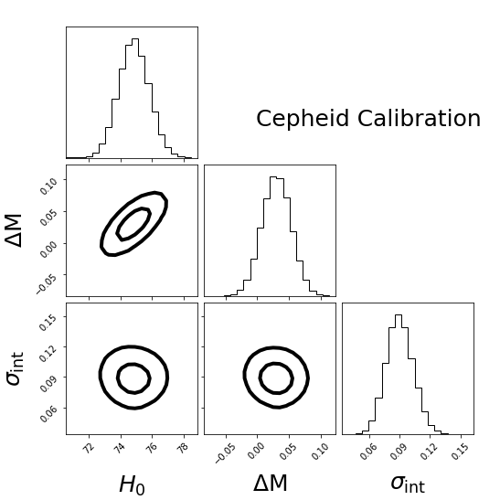
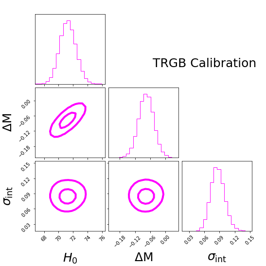
Figure 6: The corner plot showing the posterior distribution for the $H_{0}$, $M_{X}$ and $\sigma_{\rm int}$ using the Cepheid (left) and TRGB (right) calibrated distance ladder. With the Cepheid distance ladder we find $H_{0}=74.82\pm 0.97$ km ${\rm s}^{-1}\,{\rm Mpc}^{-1}$ and for the TRGB we find $H_{0}=70.92\pm 1.14$ km ${\rm s}^{-1}\,{\rm Mpc}^{-1}$ . We find a small $\sigma_{\rm int}=0.094\pm 0.013$ for the Cepheid case and $\sigma_{\rm int}=0.085\pm 0.014$ mag for the TRGB case.

3 Analysis and Results

In this section, we present the results from fitting the SNe Ia in the calibrator and Hubble flow samples and inferring $H_{0}$. A summary of the calibrator SN Ia fits and the absolute distances from the Cepheid variables is presented in Table 1. We emphasise again that since the distance ladder is constructed from the relative measurements of the calibrator and Hubble flow SNe Ia, the reference distance scale used in the model training is an arbitrary factor that does not impact the final inference on $H_{0}$, since it is absorbed into the determination of the absolute magnitude offset ($\Delta M$ as defined below).

Table 3: The Hubble flow sample used in our inference. CMB frame redshifts with peculiar velocity corrections applied (referred to here as Hubble diagram redshifts) are reported along with the fitted distance from BayeSN and the lightcurve shape and absorption parameter inferred from the model fit. We emphasise that this distance, $\mu_{\rm SN}$ is inferred from the same scaling as for the calibrator sample in Tables 1 and Table 2, hence, does not impact the final estimate of $H_{0}$. The table here is truncated for formatting reasons and is available in its entirety online.

SN	$z_{\rm HD}$	$\mu_{\rm SN}$	$\sigma_{\rm SN,fit}$	$\theta$	$A_{V}$	$\log_{10}$ Host mass	NIR at max
1999ee	0.01122	33.175	0.035	-0.291	0.712	$\ldots$	Y
1999ek	0.017821	34.196	0.040	0.143	0.710	$\ldots$	Y
2000bh	0.024195	34.889	0.044	-0.129	0.189	$\ldots$	N
2000ca	0.02391	34.987	0.034	0.189	0.039	$\ldots$	Y

For the Hubble flow sample we present the redshifts and the fitted SN Ia distances in Table 3. Typically, the heliocentric corrections to the CMB frame are done using an additive approximation such that

$$z_{\rm Hel}=z^{+}_{\rm CMB}+z_{\rm Sun}$$ (1)

However, as noted by Davis et al. (2019); Carr et al. (2021), the correct way to transform heliocentric redshifts is to multiplicatively combine the $(1+z)$ terms, i.e.

$$(1+z_{\rm Hel})=(1+z^{X}_{\rm CMB})(1+z_{\rm Sun})$$ (2)

which gives the CMB frame redshift as

$$z^{X}_{\rm CMB}=\frac{(1+z_{\rm Hel})}{(1+z_{\rm Sun})}-1$$ (3)

the difference between the additive and multiplicative formulae is exactly $z_{\rm CMB}z_{\rm Sun}$. While this effect is small at low-$z$, it becomes significant at higher redshifts. For consistency, we transform to CMB frame using equation 3.

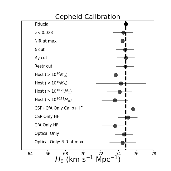
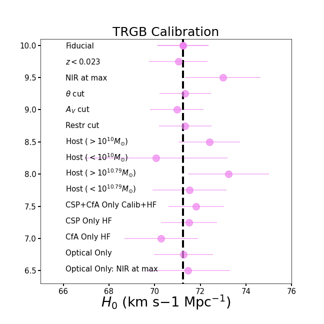
Figure 7: $H_{0}$ values for all the sample selection cases tried in this study for the Cepheid (left) and TRGB (right) calibration of the SN Ia luminosity. We note that in both calibrations the largest difference from the fiducial case is for the NIR at max subsample and the subsample with SNe Ia in low stellar mass host galaxies. The fiducial value for the Cepheid calibration is 74.82 km ${\rm s}^{-1}\,{\rm Mpc}^{-1}$ and for the TRGB is 70.92 km ${\rm s}^{-1}\,{\rm Mpc}^{-1}$ .

We then correct the redshifts for peculiar velocities using the 2M++ flow model (Carrick et al., 2015). We compare the distribution of the inferred $V$-band absorption from the host galaxy dust ($A_{V}$) and the decline rate parameters, $\theta$, between the calibrator and Hubble flow samples in Figure 3. We note that the low-reddening distribution inferred for the calibrator samples from the BayeSN inference is consistent with other methods for inferring extinction for the calibrator sample (e.g. Riess et al., 2022). We note, however, that there are no heavily extinguished ($A_{V}>1.5$) SNe in either our calibrator or Hubble flow sample. Similarly we find a larger fraction of the Hubble flow sample have $\theta>0$ (i.e. faster declining lightcurves) compared to the calibrator sample. We test what the impact of difference in the $A_{V}$ and $\theta$ distributions is on the final cosmological parameters.

Table 4: Inferred value of $H_{0}$ and the absolute luminosity offset for the fiducial case and alternate case scenarios for the Cepheid calibrated distance ladder. We also report the intrinsic scatter term and the number of SNe in each of the calibrator and Hubble flow samples in every case.

Case	$H_{0}$	$\Delta M$	$-5a$	$\sigma_{\rm int}$	$N_{\rm calib}$	$N_{\rm HF}$
	km ${\rm s}^{-1}$ ${\rm Mpc}^{-1}$	mag	mag	mag
Fiducial	74.823 $\pm$ 0.973	0.030 $\pm$ 0.023	15.660 $\pm$ 0.016	0.090${}^{+0.013}_{-0.013}$	37	67
$z<0.023$	74.532 $\pm$ 1.135	0.030 $\pm$ 0.024	15.668 $\pm$ 0.022	0.097${}^{+0.016}_{-0.015}$	37	31
NIR at max	74.440 $\pm$ 1.286	0.008 $\pm$ 0.032	15.649 $\pm$ 0.020	0.079${}^{+0.018}_{-0.016}$	15	40
$\theta$ cut	74.751 $\pm$ 1.021	0.030 $\pm$ 0.024	15.662 $\pm$ 0.018	0.094${}^{+0.015}_{-0.013}$	37	58
$A_{V}$ cut	74.821 $\pm$ 0.992	0.030 $\pm$ 0.023	15.660 $\pm$ 0.017	0.090${}^{+0.014}_{-0.013}$	37	65
Restr cut	74.756 $\pm$ 1.035	0.030 $\pm$ 0.024	15.662 $\pm$ 0.018	0.095${}^{+0.015}_{-0.014}$	37	56
Host ($>10^{10}M_{\odot}$)	73.678 $\pm$ 1.023	-0.012 $\pm$ 0.025	15.651 $\pm$ 0.016	0.068${}^{+0.015}_{-0.015}$	25	49
Host ($<10^{10}M_{\odot}$)	74.259 $\pm$ 2.842	0.119 $\pm$ 0.053	15.765 $\pm$ 0.064	0.133${}^{+0.043}_{-0.035}$	12	7
Host ($>10^{10.79}M_{\odot}$)	74.102 $\pm$ 1.441	-0.015 $\pm$ 0.037	15.636 $\pm$ 0.021	0.070${}^{+0.022}_{-0.019}$	13	32
Host ($<10^{10.79}M_{\odot}$)	73.561 $\pm$ 1.484	0.052 $\pm$ 0.031	15.718 $\pm$ 0.031	0.104${}^{+0.022}_{-0.019}$	24	22
CSP+CfA only calib+HF	75.641 $\pm$ 1.214	0.059 $\pm$ 0.031	15.666 $\pm$ 0.016	0.077${}^{+0.017}_{-0.015}$	19	58
CSP Only HF	75.056 $\pm$ 1.091	0.030 $\pm$ 0.024	15.653 $\pm$ 0.021	0.092${}^{+0.016}_{-0.015}$	37	39
CfA Only HF	73.591 $\pm$ 1.462	0.029 $\pm$ 0.026	15.695 $\pm$ 0.035	0.109${}^{+0.021}_{-0.019}$	37	19
Opt-Only	74.630 $\pm$ 1.021	0.025 $\pm$ 0.022	15.660 $\pm$ 0.020	0.088${}^{+0.016}_{-0.015}$	37	67
Opt-Only: NIR at Max	74.452 $\pm$ 1.490	0.007 $\pm$ 0.034	15.647 $\pm$ 0.026	0.087${}^{+0.023}_{-0.020}$	15	40

To infer cosmological parameters from the combination of the calibrator and Hubble flow SNe, we express the luminosity distance as a Taylor expansion in terms of time derivatives of the scale factor. First, we define the dimensionless luminosity distance as

$$\begin{split}\tilde{d}_{L}(z)={z}{\left[1+\frac{(1-q_{0})z}{2}-\frac{(1-q_{0}-3q^{2}_{0}+j_{0})z^{2}}{6}+\mathcal{O}(z^{3})\right]}\end{split}$$ (4)

where $z$ refers to the “true" cosmological redshift. The luminosity distance is then $d_{L}(z)=c\,\tilde{d}_{L}(z)/H_{0}$ and the distance modulus is $\mu(z;H_{0})=25+5\log_{10}(d_{L}(z)\,\text{Mpc}^{-1})$. We perform the standard analysis with fixed $q_{0}=-0.55$ and $j_{0}=1$. In the absence of errors, the intercept of the ridge line of the Hubble diagram is defined as

$$\begin{split}a=\log_{10}(c\,\tilde{d}_{L}(z))-0.2\times\mu_{\rm SN}.\end{split}$$ (5)

Therefore, $H_{0}$ can be written in terms of the absolute magnitude offset and the intercept of the Hubble diagram as

$$\log_{10}H_{0}=\frac{\Delta M+5a+25}{5},$$ (6)

where $\Delta M$ is the offset from the reference absolute magnitude assumed in the SN Ia model and is constrained by the calibrator sample.

For the calibrator samples, we define $\Delta\hat{\mu}_{\text{Cal},k}=\hat{\mu}_{\text{SN},k}-\hat{\mu}_{\text{Cal},k}$ where $\hat{\mu}_{\text{SN},k}$ is the SN Ia photometric distance estimate and $\hat{\mu}_{\text{Cal},k}$ is the independent calibrator distance estimate (either from Cepheids or the TRGB) to the $k$th host galaxy. Its variance is given by

$$\sigma_{{\rm Cal},k}^{2}=\sigma_{{\rm SN,fit},k}^{2}+\sigma_{{\rm Cal,}k}^{2}+\sigma_{\rm int}^{2}.$$ (7)

For the Hubble flow rung, we define $\Delta\hat{\mu}_{\text{HF},i}=\hat{\mu}_{\text{SN},i}-\mu(\hat{z}_{i};H_{0}^{\rm ref})$ where $H_{0}^{\rm ref}$ is a fixed reference value and $\hat{z}_{i}$ is the inferred redshift for the $i$th Hubble flow SN Ia host galaxy. The final posterior distributions do not depend on the choice of $H_{0}^{\rm ref}$. The variance of $\Delta\mu_{{\rm HF},i}$ is given by

$$\sigma_{{\rm HF},i}^{2}=\sigma_{{\rm SN,fit},i}^{2}+\sigma_{{\rm pec,mag},i}^{2}+\sigma_{\rm int}^{2}.$$ (8)

where

$$\sigma_{{\rm pec,mag},i}\approx\frac{5}{\ln 10}\frac{\sigma_{\rm pec}}{cz_{i}}$$ (9)

is the magnitude uncertainty due to the peculiar velocity errors. We assume a peculiar velocity uncertainty $\sigma_{\rm pec}=250\,\text{km s}^{-1}$ (e.g. Riess et al., 2022).

We therefore define the likelihood as the product of the calibrator and Hubble flow likelihoods

$$\mathcal{L}(H_{0},\Delta M,\sigma_{\rm int})=\mathcal{L_{\rm Cal}}\times\mathcal{L_{\rm HF}},$$ (10)

where the calibrator likelihood is

$$\mathcal{L}_{\rm Cal}=\prod_{k=1}^{N_{\rm Cal}}\mathcal{N}(\Delta\hat{\mu}_{\text{Cal},k}|\,\Delta M,\sigma_{\rm Cal,k}^{2}),$$ (11)

where $N_{\rm Cal}$ is the total number of calibrator host galaxies. and the Hubble flow likelihood is

$$\begin{split}\mathcal{L}_{\text{HF}}&=\prod_{i=1}^{N_{\rm HF}}\mathcal{N}(\hat{\mu}_{\text{SN},i}-\mu(\hat{z_{i}};H_{0})|\,\Delta M,\sigma_{\text{HF},i}^{2})\\ &=\prod_{i=1}^{N_{\rm HF}}\mathcal{N}(\Delta\hat{\mu}_{\text{HF},i}|\,\Delta M-5\log_{10}(H_{0}/H_{0}^{\rm ref}),\sigma_{\text{HF},i}^{2})\end{split}$$ (12)

where $N_{\rm HF}$ is the total number of Hubble flow host galaxies. Here we have used the identity $\mu(\hat{z}_{i};H_{0})=\mu(\hat{z_{i}};H_{0}^{\rm ref})-5\log_{10}(H_{0}/H_{0}^{\rm ref})$ so that $\Delta\hat{\mu}_{\text{HF},i}$ can be computed independently of $H_{0}$, while the overall likelihood is still independent of $H_{0}^{\rm ref}$. Hence, the log likelihood we use for our analysis is,

$$\begin{split}\ln\mathcal{L}(H_{0},\Delta M,\sigma_{\rm int})=&-\frac{1}{2}\sum_{k}\ln(2\pi\sigma_{{\rm Cal},k}^{2})+\frac{(\Delta\hat{\mu}_{{\rm Cal},k}-\Delta M)^{2}}{\sigma_{{\rm Cal},k}^{2}}\\ &-\frac{1}{2}\sum_{i}\ln(2\pi\sigma_{{\rm HF},i}^{2})+\frac{(\Delta\hat{\mu}_{{\rm HF},i}-\Delta M)^{2}}{\sigma_{{\rm HF},i}^{2}},\end{split}$$ (13)

The parameters $H_{0}$, $\Delta M$ and $\sigma_{\rm int}$ are inferred using an affine-invariant Markov Chain Monte Carlo as implemented by the emcee software (Foreman-Mackey et al., 2013) to sample the posterior distribution. We use 200 walkers and 20000 samples per walker with a “burn-in" of 1000 samples. For our parameter priors, we use a uniform prior between 50 and 100 km ${\rm s}^{-1}\,{\rm Mpc}^{-1}$ for $H_{0}$, between $-2$ and $2$ for $\Delta M$, and between 0 and 1 for $\sigma_{\rm int}$. We infer $a$ from each MCMC sample given $H_{0}$ and $\Delta M$, using eq 6 and for convenience we report it as -5$a$. The resulting values are plotted in figure 6. We can see that, as expected, the value of $H_{0}$ is degenerate with $\Delta M$. We find, for the fiducial case $H_{0}=74.82\pm 0.97\,{\rm km}\,{\rm s}^{-1}\,{\rm Mpc}^{-1}$, $\Delta M=0.03\pm 0.023$ mag.

Table 5: Inferred value of $H_{0}$ and the absolute luminosity offset for the fiducial case and alternate case scenarios for the TRGB calibrated distance ladder. We also report the intrinsic scatter term and the number of SNe in each of the calibrator and Hubble flow samples in every case.

Case	$H_{0}$	$\Delta M$	$-5a$	$\sigma_{\rm int}$	$N_{\rm calib}$	$N_{\rm HF}$
	km ${\rm s}^{-1}$ ${\rm Mpc}^{-1}$	mag	mag	mag
Fiducial	70.918 $\pm$ 1.149	-0.086 $\pm$ 0.030	15.660 $\pm$ 0.018	0.085${}^{+0.015}_{-0.012}$	15	67
$z<0.023$	70.710 $\pm$ 1.389	-0.085 $\pm$ 0.033	15.668 $\pm$ 0.026	0.092${}^{+0.017}_{-0.015}$	15	31
NIR at max	71.059 $\pm$ 1.557	-0.094 $\pm$ 0.042	15.648 $\pm$ 0.023	0.090${}^{+0.018}_{-0.015}$	9	40
$\theta$ cut	70.962 $\pm$ 1.185	-0.086 $\pm$ 0.031	15.659 $\pm$ 0.019	0.086${}^{+0.015}_{-0.013}$	15	62
$A_{V}$ cut	70.972 $\pm$ 1.171	-0.085 $\pm$ 0.031	15.659 $\pm$ 0.018	0.108${}^{+0.014}_{-0.012}$	15	67
Restr cut	70.984 $\pm$ 1.173	-0.085 $\pm$ 0.031	15.659 $\pm$ 0.019	0.086${}^{+0.014}_{-0.013}$	15	62
Host ($>10^{10}M_{\odot}$)	71.225 $\pm$ 1.454	-0.086 $\pm$ 0.040	15.651 $\pm$ 0.020	0.044${}^{+0.021}_{-0.019}$	7	49
Host ($<10^{10}M_{\odot}$)	70.111 $\pm$ 3.170	-0.006 $\pm$ 0.071	15.764 $\pm$ 0.069	0.137${}^{+0.053}_{-0.041}$	6	7
Host ($>10^{10.79}M_{\odot}$)	71.289 $\pm$ 1.959	-0.095 $\pm$ 0.052	15.634 $\pm$ 0.029	0.040${}^{+0.020}_{-0.028}$	5	29
Host ($<10^{10.79}M_{\odot}$)	71.608 $\pm$ 1.618	-0.023 $\pm$ 0.042	15.702 $\pm$ 0.025	0.088${}^{+0.022}_{-0.022}$	8	26
CSP+CfA only calib+HF	71.822 $\pm$ 1.536	-0.052 $\pm$ 0.043	15.666 $\pm$ 0.017	0.088${}^{+0.016}_{-0.014}$	9	58
CSP Only HF	71.188 $\pm$ 1.326	-0.085 $\pm$ 0.032	15.653 $\pm$ 0.024	0.115${}^{+0.015}_{-0.016}$	15	39
CfA Only HF	69.792 $\pm$ 1.793	-0.085 $\pm$ 0.038	15.696 $\pm$ 0.041	0.123${}^{+0.022}_{-0.019}$	15	19
Opt-Only	71.320 $\pm$ 1.248	-0.057 $\pm$ 0.033	15.679 $\pm$ 0.018	0.086${}^{+0.017}_{-0.014}$	15	67
Opt-Only: NIR at Max	71.510 $\pm$ 1.732	-0.044 $\pm$ 0.046	15.683 $\pm$ 0.024	0.105${}^{+0.023}_{-0.020}$	9	40

Similar to the method above, we fit the calibrator sample from the Carnegie Chicago Hubble program (CCHP), a total of 18 calibrator SNe Ia in 15 host galaxies (Freedman et al., 2019). A summary of the SN fit parameters and the TRGB distances is presented in Table 2. Inferring the parameters from this calibrator sample, in combination with the same Hubble flow sample as used above, we get $H_{0}=70.92\pm 1.14$ km ${\rm s}^{-1}\,{\rm Mpc}^{-1}$ and $\Delta M=-0.078\pm 0.03$ mag. Similar to the Cepheid calibration, we test the impact of alternate sample selection criteria. The summary of the constraints is presented in figure 7 and table 5.

For the fiducial case, the scatter is $\sigma_{\rm int}=0.091\pm 0.014$ mag and $0.087\pm 0.014$ mag for the Cepheid and TRGB calibration respectively. A single intrinsic scatter model can overlook systematic uncertainties. As in previous work, we test for the consistency of the dispersion in the calibrator and Hubble flow samples. We fit for two separate intrinsic scatters and find $\sigma_{\rm int,Cal}=0.117^{+0.021}_{-0.028}$ and $\sigma_{\rm int,HF}=0.067^{+0.039}_{-0.025}$ for the Cepheid calibration and $\sigma_{\rm int,Cal}=0.123^{+0.028}_{-0.034}$ and $\sigma_{\rm int,HF}=0.067^{+0.039}_{-0.026}$ for the TRGB calibration. For both methods, while the calibrator sample has higher scatter, both samples have consistent values at the $\sim 1\sigma$ level. When comparing to the single scatter model, for the Cepheid calibration, we find the central value of $H_{0}$ only changes by 0.1 km ${\rm s}^{-1}\,{\rm Mpc}^{-1}$ with a slightly larger uncertainty giving $H_{0}=74.72\pm 1.055$ km ${\rm s}^{-1}\,{\rm Mpc}^{-1}$ and the peak magnitude offset is $\Delta M=0.028\pm 0.027$ mag. For the TRGB calibration, the value of $H_{0}$ only changes by 0.05 km ${\rm s}^{-1}\,{\rm Mpc}^{-1}$ and the uncertainty increases to give $H_{0}=71.37\pm 1.33$ km ${\rm s}^{-1}\,{\rm Mpc}^{-1}$ , while the peak magnitude offset is $\Delta M=-0.071\pm 0.038$ mag. Hence, we do not find the inconsistency in the intrinsic scatter as seen previously with compilations of local SNe Ia (e.g. Dhawan et al., 2018).

3.1 Sample selection

Similar to previous studies on estimating $H_{0}$ (e.g. Dhawan et al., 2018; Burns et al., 2018; Riess et al., 2022), we test the impact of changing the fiducial sample on the final value of $H_{0}$. We describe the individual criteria here

Figure 8: Comparison of the $H_{0}$-$M$ contours for the distance ladder calibrated to the Cepheid variables (black) and the tip of the red giant branch method (violet).

$z$-cut: Alternate lower limit for the definition of the Hubble flow, with $z\geq 0.023$. This is an important test of systematics from peculiar velocity uncertainties on the final $H_{0}$ inference. While this cut only includes Hubble flow SNe Ia where the uncertainty from peculiar motions is $\sim 4\%$ or lower, it sizably reduces the Hubble flow sample.

NIR-at-Max-cut: We follow the “NIR-at-max" cut from Avelino et al. (2019). In this case, we only use the SNe that have at least one NIR observations 2.5 days or more before time of $B$-maximum, Since SNe Ia are closest to standard candles near peak in the NIR (e.g. Krisciunas et al., 2004; Phillips, 2012; Avelino et al., 2019), this subsample presents the estimate of $H_{0}$ from the best observed calibrator and Hubble flow objects. This subsample is most suited to compare the impact of adding the NIR to the data in the optical filters and hence, evaluating the improvement due to consistently modelling the optical and NIR data.

Restric-Cut: This is most restrictive cut on the dust $A_{V}$ and the lightcurve shape $\theta$ parameters to make the calibrator and Hubble flow samples as similar as possible. We restrict the Hubble flow sample to only those SNe within the range of $A_{V}$ and $\theta$ values estimated for the calibrator sample (see Figure 3). Since current calibrator and Hubble flow SNe Ia are derived from several heterogeneous surveys, the aim of this cut to mitigate the impact of different lightcurve shape and reddening distributions due to, e.g., individual survey selection effects.

Survey Subsamples: Since a large part of the Hubble flow sample is derived from either the CSP or the CfA supernova campaigns, in this cut we test the impact of using only CSP or CfA SNe for the Hubble flow rung. We also test the shift in the value when using only SNe Ia from CSP or CfA in both the calibrator and Hubble flow rungs.

Host galaxy mass: We test the impact of the host galaxy mass on the final estimate of $H_{0}$. Since there are possibilities of differing host galaxy properties between the calibrator and Hubble flow SNe Ia, e.g. because Cepheids are only found in young, star-forming galaxies, we test the impact of homogenizing the host galaxy property distribution. For this, we split the sample based on $\log_{10}(M_{\rm host}/M_{\odot})\leq,>10$ into the “low-mass" and “high-mass" subsamples, respectively. We also check the impact of the host mass split at the median mass, which we find to be 10^10.79 M_⊙ for our sample. This value is comparatively higher than the fiducial value of 10${}^{10}M_{\odot}$. For these tests, we only use the subsample of SNe Ia where host galaxy masses are available in the literature. For the Cepheid calibrator sample, this is the case for all 37 host galaxies, whereas there are 13 TRGB host galaxies with available mass estimates and a total of 55 Hubble flow SN Ia host galaxies. As not all Hubble flow host galaxies, and in the case of the TRGB calibration, not all calibrator galaxies have a stellar mass estimate, the $H_{0}$ inference from the host mass subsample cuts are not symmetrically distributed around the fiducial value, which uses the full sample.

Optical-Only: These subsamples use only the optical ($\lambda<1\,\mu$m) lightcurves for inferring the photometric distance from BayeSN. Here, we test the results for both the fiducial sample of calibrators and the subsample defined above as “NIR at max".

The results from the different cases are summarised in Tables 1 and 2. We note that out of the above cases, the largest shifts for the Cepheid calibration are for the subsample with only NIR-at-max and the low-mass sample defined with respect to the median host galaxy mass. For the TRGB calibration, the largest shifts are for the high mass subsample and the NIR at max subsamples. In both cases we see shifts of $\sim 0.7-0.8$ km ${\rm s}^{-1}\,{\rm Mpc}^{-1}$ when using only the CSP Hubble flow sample and $\sim 1.7-1.8$ km ${\rm s}^{-1}\,{\rm Mpc}^{-1}$ when using only the CfA Hubble flow sample, the latter of which is the lowest $H_{0}$ value in both calibration cases. We note that for the Cepheid calibration, there is a larger fraction of alternate cases that is below the fiducial value whereas for the TRGB case a larger fraction is above the fiducial value. We note, however, that in all these cases, the perturbations are consistent with the fiducial value, within errors, and we, therefore, conclude that these is likely to be a statistical fluctuations.

3.2 Systematic Uncertainties

In this section we quantify the systematic uncertainty on the inferred value of $H_{0}$ for both the cases with the Cepheid and TRGB calibrations.

Cepheid Calibration

: We use the sample of Cepheid calibrators from the R22 dataset. The Cepheid systematics for this dataset are at the 0.7$\%$ (Table 7 in Riess et al., 2022). We add the contribution from the standard deviation our analysis variants in Section 3.1. The total systematic error is 0.84 km ${\rm s}^{-1}\,{\rm Mpc}^{-1}$ .

TRGB calibration

: For the TRGB calibrated distance ladder, we take the systematic error from the absolute calibration of the TRGB magnitude as reported in Freedman (2021). An error in the $M_{\rm I,TRGB}$ of 0.038 mag corresponds to a $\sigma(H_{0})$ of 1.33 km ${\rm s}^{-1}\,{\rm Mpc}^{-1}$ . Similar to the case for the Cepheid calibrated distance ladder, we add the standard deviation of our analysis variants, hence, the total systematic uncertainty is 1.49 km ${\rm s}^{-1}\,{\rm Mpc}^{-1}$ .

We note that taking the standard deviation of the analysis variants is a conservative upper limit on the systematic uncertainty.

4 Discussion and Conclusions

We have presented a consistent inference of $H_{0}$ from modelling the optical to near infrared lightcurves of SNe Ia. We find $H_{0}=74.82\pm 0.97\pm 0.84$ km ${\rm s}^{-1}\,{\rm Mpc}^{-1}$   for the Cepheid calibration and $H_{0}=70.92\pm 1.14\pm 1.49$ km ${\rm s}^{-1}\,{\rm Mpc}^{-1}$   for the TRGB calibration.= These value of $H_{0}$ and $\sim 1-1.5$ km ${\rm s}^{-1}\,{\rm Mpc}^{-1}$ higher than the cases estimated in the literature, using optical only data for SNe Ia (Riess et al., 2022; Freedman, 2021). This is also seen in other studies incorporating the NIR SN Ia data (e.g. Galbany et al., 2022). We note that while the Cepheid calibration measurement is in a significant (4.9$\sigma$) tension with the early universe inference from Planck Collaboration (2020), the TRGB measurement has a greater consistency with the early universe inference (1.8$\sigma$ tension). The level of tension for each of the two probes is very similar to reported degrees of tension in the literature (e.g., Freedman, 2021; Riess et al., 2022).

We test the impact of various analysis assumptions for both the calibrator and Hubble flow samples for both the Cepheid and TRGB calibrations. We find that for the Cepheid calibration, the alternate assumptions do not change the central value of $H_{0}$ significantly. However, in the cases of low host galaxy mass subsample the uncertainty is more than twice larger which is due mostly to a smaller number of SNe in the sample. For the $A_{V}$ and $\theta$ cuts as well as the Restrictive cut applied in the sample, the TRGB calibrators have a more similar distribution to the Hubble flow compared to the Cepheid calibrators.

We test the impact of simultaneous modelling of the optical and the NIR by fitting only the optical filters for both the calibrator and the Hubble flow sample. For the complete sample, we do not find any significant shift in the value of $H_{0}$ from the optical only, with respect to the fiducial case. Moreover, for the complete sample, the improvement in the final $H_{0}$ estimate is marginal. We attribute this to the the dominant source of uncertainty arising from the small number of calibrator SNe Ia. Additionally since both the calibrator and Hubble flow SNe Ia have densely sampled lightcurves, we compare the $H_{0}$ estimate and uncertainty from only the NIR-at-max subsample. The $H_{0}$ constraint from this subsample is up to $\sim$15% more precise than the constraint from only fitting the optical lightcurves for the same subsample. This is a promising sign for using consistent modelling of SNe Ia lightcurves from the optical to the NIR, even for high-$z$ SN cosmology studies, e.g. with the RAISIN survey (Jones et al., 2022).

There have been debates in the literature as to whether effects of host galaxy environment can highly bias the inferred $H_{0}$ (Rigault et al., 2020; Jones et al., 2018). Here we tested the impact of the environment by dividing the samples into low- and high-mass host galaxies In the first case, we divide the sample in mass bins above or below 10¹⁰ M_⊙, as done previously in the literature (e.g. Riess et al., 2022). While the value of $H_{0}$ is shifted in the low-mass sample compared to the fiducial analyses, the uncertainty is larger due to the small number of SNe Ia in the subsample in the current analyses. Hence, it will be crucial to test this effect with SN Ia samples (both in the calibrator and Hubble flow) derived from untargeted surveys such as ZTF (Dhawan et al., 2022a) and YSE (Jones et al., 2021). Moreover, we note that the high host mass subsample has a lower $\sigma_{\rm int}$. The SN Ia datasets from untargeted surveys will be critical to understand what the origin of such a low scatter is.

Aspects of our analysis can be improved in terms of both statistical and systematic uncertainties. Our statistical uncertainties would be improved with a larger number of SNe in both the calibrator and Hubble flow datasets. In the near future, observatories like the James Webb Space Telescope have the capabilities to observe host galaxies of SNe Ia in the local volume out to $\sim 80$  Mpc, significantly larger than the farthest calibrator galaxy in the current sample at $\sim 40$  Mpc (e.g. Riess et al., 2022). This can increase the calibrator sample from a few tens of SNe Ia to $>100$ SNe Ia, when using methods like the TRGB which are “single-shot" and do not require multiple visits per galaxy to get an accurate distance. Having such an untargeted sample will also be important for testing the impact of host galaxy properties on the inferred $H_{0}$, since the current Hubble flow sample has small number statistics in the low mass bin. We note, additionally, that in this analysis we use the most updated calibration of the Cepheid and TRGB methods. However, there are alternate assumptions in the more nearby rungs of the Cepheid (Mörtsell et al., 2022a, b) or TRGB (Anand et al., 2022) distance ladder, e.g. a 0.05 mag brighter (fainter) shift in the absolute magnitude would propagate throughout the distance ladder measurement as a shift in $H_{0}$ of $\sim$ 1.6 km ${\rm s}^{-1}\,{\rm Mpc}^{-1}$ lower (higher), (e.g., see Li et al., 2022, for a summary of the absolute calibration of the TRGB). Moreover, our current analysis uses peculiar velocity corrections from the 2M++ flow model as described in Carrick et al. (2015). Recent improvements in the corrections can further help reduce the uncertainty in the inferred $H_{0}$ (Peterson et al., 2021; Kenworthy et al., 2022).

There are possibilities to reduce systematic uncertainties in the future. Improving the BayeSN model by retraining using an updated set of NIR spectra (e.g. Lu et al., 2022) can further reduce uncertainties in the inferred distances from the SED model. Since we required a dataset with both optical and NIR coverage, the median redshift of the sample is typically lower than that of samples in the literature. A sample with higher median $z$ would be less prone to systematics from peculiar velocities. A higher median redshift is one of salient features of SN Ia programs optimised for the NIR, e.g. SIRAH (Jha et al., 2019). In addition, for our work, we use a fixed global value of the dust $R_{V}$ for all objects. However, we can use joint optical and NIR data to estimate $R_{V}$ (Krisciunas et al., 2007; Mandel et al., 2011; Burns et al., 2014). Such optical-NIR constraints will be important to probe potential differences in intrinsic or dust properties in various SN Ia host galaxy environments (e.g., Uddin et al., 2020; Brout & Scolnic, 2021; Johansson et al., 2021; Thorp et al., 2021; Thorp & Mandel, 2022) and test the impact of possible differences on the inferred value of $H_{0}$. Moreover, some of the surveys that observed SNe in our sample were targeted to particular galaxy types. Modelling a uniform distance ladder with both calibrator and Hubble flow SNe Ia discovered and followed-up with the same survey could reduce this source of systematic error (e.g. Dhawan et al., 2022b). Our results show potential pathways to reduce uncertainties in the measurement of a key cosmological parameter, $H_{0}$, with future large samples of SNe Ia.

Data Availability

All data used in this manuscript are publicly available from the sources described in §2.

References

- Anand et al. (2022) Anand G. S., Tully R. B., Rizzi L., Riess A. G., Yuan W., 2022, ApJ, 932, 15
- Avelino et al. (2019) Avelino A., Friedman A. S., Mandel K. S., Jones D. O., Challis P. J., Kirshner R. P., 2019, ApJ, 887, 106
- Barone-Nugent et al. (2012) Barone-Nugent R. L., et al., 2012, MNRAS, 425, 1007
- Betancourt (2016) Betancourt M., 2016, arXiv e-prints, p. arXiv:1601.00225
- Brout & Scolnic (2021) Brout D., Scolnic D., 2021, ApJ, 909, 26
- Brout et al. (2021) Brout D., et al., 2021, arXiv e-prints, p. arXiv:2112.03864
- Burns et al. (2011) Burns C. R., et al., 2011, AJ, 141, 19
- Burns et al. (2014) Burns C. R., et al., 2014, ApJ, 789, 32
- Burns et al. (2018) Burns C. R., et al., 2018, ApJ, 869, 56
- Carpenter et al. (2017) Carpenter B., et al., 2017, Journal of Statistical Software, 76, 1
- Carr et al. (2021) Carr A., Davis T. M., Scolnic D., Said K., Brout D., Peterson E. R., Kessler R., 2021, arXiv e-prints, p. arXiv:2112.01471
- Carrick et al. (2015) Carrick J., Turnbull S. J., Lavaux G., Hudson M. J., 2015, MNRAS, 450, 317
- Cartier et al. (2014) Cartier R., et al., 2014, ApJ, 789, 89
- Contreras et al. (2018) Contreras C., et al., 2018, ApJ, 859, 24
- Davis et al. (2019) Davis T. M., Hinton S. R., Howlett C., Calcino J., 2019, MNRAS, 490, 2948
- Dhawan et al. (2018) Dhawan S., Jha S. W., Leibundgut B., 2018, A&A, 609, A72
- Dhawan et al. (2022a) Dhawan S., et al., 2022a, MNRAS, 510, 2228
- Dhawan et al. (2022b) Dhawan S., et al., 2022b, ApJ, 934, 185
- Elias et al. (1981) Elias J. H., Frogel J. A., Hackwell J. A., Persson S. E., 1981, ApJ, 251, L13
- Elias et al. (1985) Elias J. H., Matthews K., Neugebauer G., Persson S. E., 1985, ApJ, 296, 379
- Fitzpatrick (1999) Fitzpatrick E. L., 1999, PASP, 111, 63
- Folatelli et al. (2010) Folatelli G., et al., 2010, AJ, 139, 120
- Foreman-Mackey et al. (2013) Foreman-Mackey D., Hogg D. W., Lang D., Goodman J., 2013, PASP, 125, 306
- Freedman (2021) Freedman W. L., 2021, ApJ, 919, 16
- Freedman et al. (2019) Freedman W. L., et al., 2019, ApJ, 882, 34
- Friedman et al. (2015) Friedman A. S., et al., 2015, ApJS, 220, 9
- Galbany et al. (2022) Galbany L., et al., 2022, arXiv e-prints, p. arXiv:2209.02546
- Gall et al. (2018) Gall C., et al., 2018, A&A, 611, A58
- Guy et al. (2007) Guy J., et al., 2007, A&A, 466, 11
- Hamuy et al. (1991) Hamuy M., Phillips M. M., Maza J., Wischnjewsky M., Uomoto A., Landolt A. U., Khatwani R., 1991, AJ, 102, 208
- Hoffman & Gelman (2014) Hoffman M. D., Gelman A., 2014, J. Machine Learning Res., 15, 1593
- Hounsell et al. (2018) Hounsell R., et al., 2018, ApJ, 867, 23
- Jha et al. (1999) Jha S., et al., 1999, ApJS, 125, 73
- Jha et al. (2019) Jha S. W., et al., 2019, Supernovae in the Infrared avec Hubble, HST Proposal. Cycle 27, ID. #15889
- Johansson et al. (2021) Johansson J., et al., 2021, ApJ, 923, 237
- Jones et al. (2018) Jones D. O., et al., 2018, ApJ, 867, 108
- Jones et al. (2021) Jones D. O., et al., 2021, ApJ, 908, 143
- Jones et al. (2022) Jones D. O., et al., 2022, ApJ, 933, 172
- Kattner et al. (2012) Kattner S., et al., 2012, PASP, 124, 114
- Kenworthy et al. (2022) Kenworthy W. D., et al., 2022, ApJ, 935, 83
- Knox & Millea (2020) Knox L., Millea M., 2020, Phys. Rev. D, 101, 043533
- Konchady et al. (2022) Konchady T., Oelkers R. J., Jones D. O., Yuan W., Macri L. M., Peterson E. R., Riess A. G., 2022, ApJS, 258, 24
- Krisciunas et al. (2000) Krisciunas K., Hastings N. C., Loomis K., McMillan R., Rest A., Riess A. G., Stubbs C., 2000, ApJ, 539, 658
- Krisciunas et al. (2003) Krisciunas K., et al., 2003, AJ, 125, 166
- Krisciunas et al. (2004) Krisciunas K., Phillips M. M., Suntzeff N. B., 2004, ApJ, 602, L81
- Krisciunas et al. (2007) Krisciunas K., et al., 2007, AJ, 133, 58
- Krisciunas et al. (2017) Krisciunas K., et al., 2017, AJ, 154, 211
- Leibundgut et al. (1991) Leibundgut B., Kirshner R. P., Filippenko A. V., Shields J. C., Foltz C. B., Phillips M. M., Sonneborn G., 1991, ApJ, 371, L23
- Li et al. (2022) Li S., Casertano S., Riess A. G., 2022, ApJ, 939, 96
- Lu et al. (2022) Lu J., et al., 2022, arXiv e-prints, p. arXiv:2211.05998
- Mandel et al. (2009) Mandel K. S., Wood-Vasey W. M., Friedman A. S., Kirshner R. P., 2009, ApJ, 704, 629
- Mandel et al. (2011) Mandel K. S., Narayan G., Kirshner R. P., 2011, ApJ, 731, 120
- Mandel et al. (2022) Mandel K. S., Thorp S., Narayan G., Friedman A. S., Avelino A., 2022, MNRAS, 510, 3939
- Marion et al. (2016) Marion G. H., et al., 2016, ApJ, 820, 92
- Matheson et al. (2012) Matheson T., et al., 2012, ApJ, 754, 19
- Meikle (2000) Meikle W. P. S., 2000, MNRAS, 314, 782
- Mörtsell et al. (2022a) Mörtsell E., Goobar A., Johansson J., Dhawan S., 2022a, ApJ, 933, 212
- Mörtsell et al. (2022b) Mörtsell E., Goobar A., Johansson J., Dhawan S., 2022b, ApJ, 935, 58
- Müller-Bravo et al. (2022) Müller-Bravo T. E., et al., 2022, A&A, 665, A123
- Peterson et al. (2021) Peterson E. R., et al., 2021, arXiv e-prints, p. arXiv:2110.03487
- Phillips (2012) Phillips M. M., 2012, Publ. Astron. Soc. Australia, 29, 434
- Phillips et al. (2019) Phillips M. M., et al., 2019, PASP, 131, 014001
- Planck Collaboration (2020) Planck Collaboration 2020, A&A, 641, A6
- Richmond & Smith (2012) Richmond M. W., Smith H. A., 2012, JAAVSO, 40, 872
- Richmond et al. (1995) Richmond M. W., et al., 1995, AJ, 109, 2121
- Riess et al. (1999) Riess A. G., et al., 1999, AJ, 118, 2675
- Riess et al. (2005) Riess A. G., et al., 2005, ApJ, 627, 579
- Riess et al. (2016) Riess A. G., et al., 2016, ApJ, 826, 56
- Riess et al. (2022) Riess A. G., et al., 2022, ApJ, 934, L7
- Rigault et al. (2020) Rigault M., et al., 2020, A&A, 644, A176
- Rose et al. (2021) Rose B. M., et al., 2021, arXiv e-prints, p. arXiv:2111.03081
- Schöneberg et al. (2022) Schöneberg N., Abellán G. F., Sánchez A. P., Witte S. J., Poulin V., Lesgourgues J., 2022, Phys. Rep., 984, 1
- Schweizer et al. (2008) Schweizer F., et al., 2008, AJ, 136, 1482
- Scolnic et al. (2021) Scolnic D., et al., 2021, arXiv e-prints, p. arXiv:2112.03863
- Shah et al. (2021) Shah P., Lemos P., Lahav O., 2021, A&ARv, 29, 9
- Silverman et al. (2012) Silverman J. M., et al., 2012, MNRAS, 425, 1789
- Stan Development Team (2020) Stan Development Team 2020, Stan Modelling Language Users Guide and Reference Manual v.2.25. https://mc-stan.org
- Stritzinger et al. (2010) Stritzinger M., et al., 2010, AJ, 140, 2036
- Stritzinger et al. (2011) Stritzinger M. D., et al., 2011, AJ, 142, 156
- Thorp & Mandel (2022) Thorp S., Mandel K. S., 2022, MNRAS, 517, 2360
- Thorp et al. (2021) Thorp S., Mandel K. S., Jones D. O., Ward S. M., Narayan G., 2021, MNRAS, 508, 4310
- Tsvetkov (1982) Tsvetkov D. Y., 1982, Soviet Astronomy Letters, 8, 115
- Uddin et al. (2020) Uddin S. A., et al., 2020, ApJ, 901, 143
- Walker & Marino (1982) Walker W. S. G., Marino B. F., 1982, Royal Astronomical Society of New Zealand Publications of Variable Star Section, 10, 53
- Ward et al. (2022) Ward S. M., et al., 2022, arXiv e-prints, p. arXiv:2209.10558
- Wells et al. (1994) Wells L. A., et al., 1994, AJ, 108, 2233
- Weyant et al. (2014) Weyant A., Wood-Vasey W. M., Allen L., Garnavich P. M., Jha S. W., Joyce R., Matheson T., 2014, ApJ, 784, 105
- Weyant et al. (2018) Weyant A., et al., 2018, AJ, 155, 201
- Wood-Vasey et al. (2008) Wood-Vasey W. M., et al., 2008, ApJ, 689, 377