Probing quasar lifetimes with proximate $21$-centimetre absorption in the diffuse intergalactic medium at redshifts $z\geq 6$

Abstract

Enhanced ionizing radiation in close proximity to redshift $z\gtrsim 6$ quasars creates short windows of intergalactic Ly$\alpha$ transmission blueward of the quasar Ly$\alpha$ emission lines. The majority of these Ly$\alpha$ near-zones are consistent with quasars that have optically/UV bright lifetimes of $t_{\rm Q}\sim 10^{5}-10^{7}\rm\,yr$. However, lifetimes as short as $t_{\rm Q}\lesssim 10^{4}\rm\,yr$ appear to be required by the smallest Ly$\alpha$ near-zones. These short lifetimes present an apparent challenge for the growth of $\sim 10^{9}\rm\,M_{\odot}$ black holes at $z\gtrsim 6$. Accretion over longer timescales is only possible if black holes grow primarily in an obscured phase, or if the quasars are variable on timescales comparable to the equilibriation time for ionized hydrogen. Distinguishing between very young quasars and older quasars that have experienced episodic accretion with Ly$\alpha$ absorption alone is challenging, however. We therefore predict the signature of proximate 21-cm absorption around $z\gtrsim 6$ radio-loud quasars. For modest pre-heating of intergalactic hydrogen by the X-ray background, where the spin temperature $T_{\rm S}\lesssim 10^{2}\rm\,K$ prior to any quasar heating, we find proximate 21-cm absorption should be observable in the spectra of radio-loud quasars. The extent of the proximate 21-cm absorption is sensitive to the integrated lifetime of the quasar. Evidence for proximate 21-cm absorption from the diffuse intergalactic medium within $2-3\rm\,pMpc$ of a (radio-loud) quasar would be consistent with a short quasar lifetime, $t_{\rm Q}\lesssim 10^{5}\rm\,yr$, and would provide a complementary constraint on models for high redshift black hole growth.

1 Introduction

The intergalactic medium (IGM) becomes opaque to Ly$\alpha$ photons approaching the end stages of reionization at $z\gtrsim 5.5$, when the average neutral hydrogen fraction $\langle x_{\rm HI}\rangle\gtrsim 10^{-4}$ (for a review see Becker et al., 2015a). However, in close proximity to highly luminous quasars at $z\gtrsim 5.5$, local enhancements in the ionizing radiation field leave short windows of Ly$\alpha$ transmission blueward of the quasar Ly$\alpha$ emission line. These regions – referred to as Ly$\alpha$ near-zones or proximity zones – are typically $1$–$10$ proper Mpc (pMpc) in extent (Fan et al., 2006; Carilli et al., 2010; Willott et al., 2010; Venemans et al., 2015; Reed et al., 2015; Eilers et al., 2017, 2021; Mazzucchelli et al., 2017; Ishimoto et al., 2020). Several near-zones at $z\simeq 7$ also exhibit evidence for Ly$\alpha$ damping wings that extend redward of the quasar systemic redshift (Mortlock et al., 2011; Bañados et al., 2018; Wang et al., 2020; Yang et al., 2020a), which is expected if the surrounding IGM is substantially neutral (Miralda-Escudé & Rees, 1998). Early work suggested that Ly$\alpha$ near-zones may be tracing quasar H$\,\rm\scriptstyle II$ regions embedded in an otherwise largely neutral IGM (e.g. Shapiro & Giroux, 1987; Cen & Haiman, 2000; Madau & Rees, 2000; Wyithe & Loeb, 2004a). Subsequent radiative transfer modelling (Bolton & Haehnelt, 2007; Maselli et al., 2007; Lidz et al., 2007; Wyithe et al., 2008) demonstrated a more complex picture, where the Ly$\alpha$ near-zones at $z\simeq 6$ may also be explained if the quasars are surrounded by a highly ionized IGM – analogous to the classical proximity effect at lower redshift (e.g. Murdoch et al., 1986; Bajtlik et al., 1988).

In the last decade the number of $z\gtrsim 6$ quasar spectra with well measured Ly$\alpha$ near-zone sizes has grown considerably. Over $280$ quasars at $z>6$ have now been discovered (see e.g. Bosman, 2022). Submillimetre observations have provided improved measurements of quasar systemic redshifts, yielding better estimates of the Ly$\alpha$ near-zone sizes (Eilers et al., 2021). After correcting for differences in the intrinsic luminosity of the quasars, the scatter in the $\sim 80$ published Ly$\alpha$ near-zone sizes can be largely explained by a combination of cosmic variance (Keating et al., 2015), differences in the optically/UV bright lifetime of the quasars (Morey et al., 2021), and perhaps the occasional proximate high column density absorption system (Chen & Gnedin, 2021). The observed Ly$\alpha$ near-zone size distribution is reasonably well reproduced if a highly ionized IGM surrounds the quasars at $z\simeq 6$ (Wyithe et al., 2008; Morey et al., 2021). However, the Ly$\alpha$ damping wings in the spectra of several $z>7$ quasars are suggestive of a substantially more neutral IGM by $z\simeq 7$, such that $\langle x_{\rm HI}\rangle>0.1$, (Bolton et al., 2011; Greig et al., 2017, 2022; Davies et al., 2018, but see also Bosman & Becker (2015)).

Several recent studies have focused on constraining optically/UV bright quasar lifetimes, $t_{\rm Q}$, from the Ly$\alpha$ near-zone data at $z\simeq 6$. Morey et al. (2021) find an average optically/UV bright lifetime of $t_{\rm Q}\sim 10^{6}\rm\,yr$ is consistent with the transmission profiles of most Ly$\alpha$ near-zones at $z\simeq 6$. Eilers et al. (2017, 2021) have furthermore presented several very small Ly$\alpha$ near-zones with luminosity corrected sizes of $\lesssim 1\rm\,pMpc$, consistent with optically/UV bright lifetimes of $t_{\rm Q}\lesssim 10^{4}$–$10^{5}\rm\,yr$. These small Ly$\alpha$ near-zones represent $\lesssim 10$ per cent of all quasar Ly$\alpha$ near-zones at $z\simeq 6$. However, if the black holes powering these quasars accrete most of their mass when the quasars are optically/UV bright, such a short average lifetime is in significant tension with the build up of $\sim 10^{9}\rm\,M_{\odot}$ supermassive black holes by $z=6$; the e-folding time for Eddington limited accretion is at least an order of magnitude larger. Possible solutions are radiatively inefficient, mildly super-Eddington accretion (Madau et al., 2014; Davies et al., 2019; Kroupa et al., 2020), black holes that grow primarily in an obscured, optically/UV faint phase (Hopkins et al., 2005; Ricci et al., 2017) or episodic accretion that produces “flickering” quasar light curves (Schawinski et al., 2015; Davies et al., 2020).

Observationally distinguishing between very young quasars and older quasars that have experienced episodic or obscured accretion with Ly$\alpha$ near-zones is challenging, however. Another possibility is detecting the 21-cm signal from neutral hydrogen around the quasars. In principle, if the foregrounds can be accurately removed, the sizes of quasar H$\,\rm\scriptstyle II$ regions may be measured directly with 21-cm tomography; the neutral, X-ray heated hydrogen outside of the quasar H$\,\rm\scriptstyle II$ region should appear in emission against the radio background (e.g. Wyithe & Loeb, 2004b; Kohler et al., 2005; Rhook & Haehnelt, 2006; Geil & Wyithe, 2008; Majumdar et al., 2012; Datta et al., 2012; Kakiichi et al., 2017; Ma et al., 2020; Davies et al., 2021). Assuming the recombination timescale $t_{\rm rec}\gg t_{\rm Q}$, 21-cm tomography measurements would enable a direct determination of the quasar age, because the H$\,\rm\scriptstyle II$ region size $R_{\rm HII}\propto t_{\rm Q}^{1/3}$ (see e.g. Eq. (12) later). A related approach that has received less attention is to instead consider the forest of redshifted 21-cm absorption expected from the neutral IGM in the spectra of radio-loud background sources at $z\gtrsim 6$ (for recent examples of potential background sources, see e.g. Belladitta et al., 2020; Ighina et al., 2021; Bañados et al., 2021; Liu et al., 2021). Unlike tomography, observing the IGM in 21-cm absorption allows small-scale IGM structure to be resolved and it is (in principle) a simpler observation that does not rely on the removal of challenging foregrounds (see e.g. Carilli et al., 2002; Furlanetto & Loeb, 2002; Furlanetto, 2006a; Meiksin, 2011; Xu et al., 2011; Ciardi et al., 2013; Semelin, 2016; Villanueva-Domingo & Ichiki, 2022).

Šoltinský et al. (2021) recently discussed the detectability of the 21-cm forest in the context of the late ($z\simeq 5.3$) reionization models (e.g. Kulkarni et al., 2019; Keating et al., 2020; Nasir & D’Aloisio, 2020; Qin et al., 2021; Choudhury et al., 2021) that appear to be favoured by the large variations found in the Ly$\alpha$ forest effective optical depth at $z>5$ (Becker et al., 2015b; Eilers et al., 2018; Yang et al., 2020b; Bosman et al., 2018; Bosman et al., 2022). Šoltinský et al. (2021) noted that, for modest X-ray pre-heating, such that the IGM spin temperature $T_{\rm S}\lesssim 10^{2}\rm\,K$, strong 21-cm forest absorption with optical depths $\tau_{21}\geq 10^{-2}$ will persist until $z=6$ in late reionization models. A null detection of the 21-cm forest at $z=6$ would also place useful limits on the soft X-ray background. Toward higher redshifts, $z>7$, strong 21-cm forest absorbers will become significantly more abundant, particularly if the spin and kinetic temperatures are not tightly coupled (see e.g. fig. 7 in Šoltinský et al. (2021)).

In this context, Bañados et al. (2021) have recently reported the discovery of a radio-loud quasar PSO J172$+$18 at $z=6.82$, with an absolute AB magnitude $M_{1450}=-25.81$ and an optical/near-infrared spectrum that exhibits a Ly$\alpha$ near-zone size $R_{\rm Ly\alpha}=3.96\pm 0.48\rm\,pMpc$. This raises the intriguing possibility of also obtaining a radio spectrum from this or similar objects with low frequency radio interferometry arrays (see also e.g. Gloudemans et al., 2022). For spin temperatures of $T_{\rm S}\sim 10^{2}\rm\,K$ in the pre-reionization IGM, in late reionization scenarios there will be proximate 21-cm absorption from neutral islands in the diffuse IGM that will approximately trace the extent of the quasar H$\,\rm\scriptstyle II$ region. If this proximate 21-cm absorption is detected, either for an individual radio-loud quasar or within a population of objects, it would provide another possible route to constraining the lifetime of high redshift quasars. In particular, when combined with Ly$\alpha$ near-zone sizes, such a measurement could help distinguish between quasars that are very young (as is suggested if taking the Eilers et al. (2017, 2021) Ly$\alpha$ near-zone data at face value), or that are much older and have only recently transitioned to an optically/UV bright phase.

Our goal is to explore this possibility by modelling the properties of proximate 21-cm absorbers in the diffuse IGM around (radio-loud) quasars. We do this by building on the simulation framework presented in Šoltinský et al. (2021), who used the Sherwood-Relics simulations (see Puchwein et al., 2022) of inhomogeneous, late reionization to predict the properties of the 21-cm forest. In this work, we now additionally couple Sherwood-Relics with a line of sight radiative transfer code that simulates the photo-ionization and photo-heating around bright quasars (for similar approaches see e.g. Bolton & Haehnelt, 2007; Lidz et al., 2007; Davies et al., 2020; Chen & Gnedin, 2021; Satyavolu et al., 2022).

We begin by describing our fiducial quasar spectral energy distribution and the effect of the quasar UV and soft X-ray radiation on proximate Ly$\alpha$ and 21-cm absorption using a simplified, homogeneous IGM model in Section 2. We then introduce a more realistic model by using the Sherwood-Relics simulations in Section 3, and validate our model by comparing the predicted Ly$\alpha$ near-zone sizes in our simulations to observational data. Our predictions for the extent of the proximate 21-cm absorption around $z\geq 6$ quasars for a constant “light bulb” quasar emission model are presented in Section 4. In Section 5 we then extend this model to include “flickering” quasar light curves that may be appropriate for episodic black hole accretion, and discuss the implications for constraining quasar lifetimes and black hole growth. Finally, we summarise and conclude in Section 6. Supplementary information may be found in the Appendices at the end of the paper.

2 Quasar radiative transfer model

2.1 The quasar spectral energy distribution

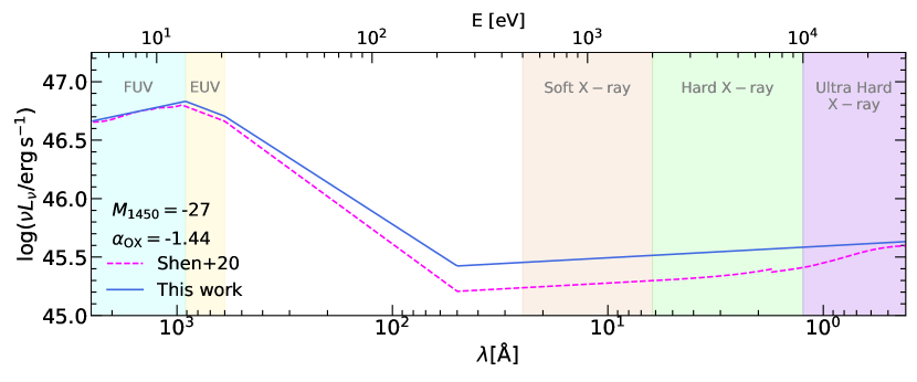
Figure 1: The fiducial power-law quasar SED used in this work (solid blue curve) compared to the SED template from Shen et al. (2020) (dashed fuchsia curve). Both SEDs are normalised at $1450\,$\mathrm{\text{\r{A}}}$$ to correspond to an absolute AB magnitude $M_{1450}=-27$. The SED is modelled as a broken power law, $f_{\nu}\propto\nu^{\alpha}$, with spectral index $\alpha_{\rm FUV}=-0.61$ between $\lambda=912\,$\mathrm{\text{\r{A}}}$-2500\,$\mathrm{\text{\r{A}}}$$ (far UV), $\alpha_{\rm EUV}=-1.70$ between $\lambda=600\,$\mathrm{\text{\r{A}}}$-912\,$\mathrm{\text{\r{A}}}$$ (extreme UV) and $\alpha_{\rm X}=-0.9$ at $\lambda\leq 50\,$\mathrm{\text{\r{A}}}$$ (X-ray). The X-ray part of the spectrum is normalized with an optical-to-X-ray spectral index of $\alpha_{\rm OX}=-1.44$. The SED between $\lambda=50\,$\mathrm{\text{\r{A}}}$-600\,$\mathrm{\text{\r{A}}}$$ connects the UV and X-ray sections of the spectrum. The shaded regions indicate common wavelength bands. Our fiducial model corresponds to an ionizing photon emission rate of $\dot{N}=1.64\times 10^{57}\rm\,s^{-1}$.

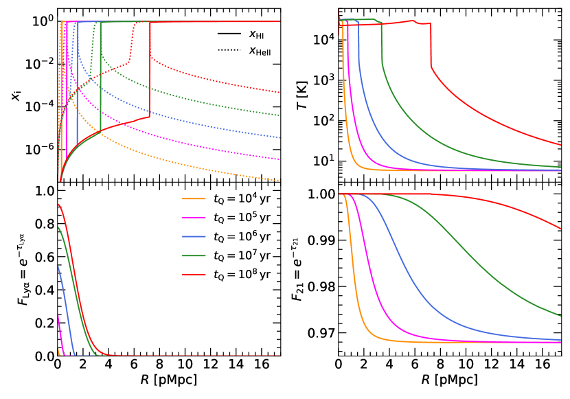
Figure 2: Radiative transfer simulation of UV and X-ray photons emitted by a quasar into a uniform density field with $\Delta=\rho/\langle\rho\rangle=1$ at $z=7$. The hydrogen and helium gas is assumed to be initially cold and neutral, and the quasar has an absolute AB magnitude $M_{\rm 1450}=-27$ (corresponding to an ionizing photon emissivity of $\dot{N}=1.64\times 10^{57}\rm\,s^{-1}$ for our fiducial SED in Fig. 1). Curves with different colours show different values for the optically/UV bright lifetime of the quasar, $t_{\rm Q}$, as indicated in the lower left panel. Upper left: the H$\,\rm\scriptstyle I$ fraction (solid curves, $x_{\rm HI}=n_{\rm HI}/n_{\rm H}$) and He$\,\rm\scriptstyle II$ fraction (dotted curves, $x_{\rm HeII}=n_{\rm HeII}/n_{\rm He}$). Upper right: the gas kinetic temperature $T$. We assume strong coupling of the spin temperature in the vicinity of the quasar, such that the spin temperature $T_{\rm S}=T$. Lower left: the Ly$\alpha$ transmission, $F_{\rm Ly\alpha}=e^{-\tau_{\rm Ly\alpha}}$. Lower right: the 21-cm transmission, $F_{21}=e^{-\tau_{21}}$.

The effect of UV and X-ray ionizing photons emitted by quasars on the high redshift IGM is simulated using the 1D multi-frequency radiative transfer (RT) calculation first described by Bolton & Haehnelt (2007), and subsequently updated in Knevitt et al. (2014) to include X-rays and secondary ionizations by fast photo-electrons (Furlanetto & Stoever, 2010). In brief, as an input this model takes the gas overdensity $\Delta$, peculiar velocity $v_{\rm pec}$, neutral hydrogen fraction $x_{\rm HI}$, gas temperature $T$, and background photo-ionization rate $\Gamma_{\rm HI}$, from sight lines drawn through a hydrodynamical simulation (see Section 3.1 for further details). We assume a spectral energy distribution (SED) for the quasar, and follow the RT of ionizing photons through hydrogen and helium gas along a large number of individual sight lines, all of which start at the position of a halo. Our RT simulations track ionizing photons emitted by the quasar at energies between $13.6\rm\,eV$ and $30\rm\,keV$, using 80 logarithmically spaced photon energy bins.

We model the quasar SED as a broken power law, $f_{\nu}\propto\nu^{\alpha}$, as shown in Fig. 1 (blue solid curve). Our choice of SED is similar to the template from Shen et al. (2020) (dashed fuchsia curve). To construct the UV part of the SED, we follow Lusso et al. (2015) and assume a spectral index $\alpha_{\rm FUV}=-0.61$ at $912\,$\mathrm{\text{\r{A}}}$\leq\lambda\leq 2500\,$\mathrm{\text{\r{A}}}$$ and $\alpha_{\rm EUV}=-1.70$ at $600\,$\mathrm{\text{\r{A}}}$\leq\lambda\leq 912\,$\mathrm{\text{\r{A}}}$$. We choose the spectral index at X-ray energies ($\lambda\leq 50\,$\mathrm{\text{\r{A}}}$$) to be $\alpha_{\rm X}=-0.9$, to approximately match the shape of the Shen et al. (2020) SED. The X-ray part of the SED is normalised using the observed correlation between the specific luminosities $L_{\nu}(2500\,$\mathrm{\text{\r{A}}}$)$ and $L_{\nu}(2\rm\,keV)$, typically parameterised by the optical-to-X-ray spectral index (Steffen et al., 2006; Lusso et al., 2010)

$$\alpha_{\rm OX}=\frac{\mathrm{log}(L_{\nu}(2\rm\,keV))-\mathrm{log}(L_{\nu}(2500\,$\mathrm{\text{\r{A}}}$))}{\mathrm{log}(\nu(2\rm\,keV))-\mathrm{log}(\nu(2500\,$\mathrm{\text{\r{A}}}$))}.$$ (1)

We assume a fiducial value of $\alpha_{\rm OX}=-1.44$ in this work, but vary this by $\Delta\alpha_{\rm OX}=0.3$ to account for a range of $L_{\nu}(2500\,$\mathrm{\text{\r{A}}}$)$ values. Our fiducial $\alpha_{\rm OX}$ is similar to the best fit value of $\alpha_{\rm OX}=-1.45\pm 0.11$ recently inferred by Connor et al. (2021) for a radio-loud quasar at $z=5.831$. Finally, the spectral shape at $\lambda=50\,$\mathrm{\text{\r{A}}}$-600\,$\mathrm{\text{\r{A}}}$$ is obtained by connecting the UV and X-ray parts of the SED.

For ease of comparison with previous literature (Eilers et al., 2017; Davies et al., 2020), we adopt a normalisation for the quasar SED corresponding to an absolute AB magnitude at $1450\,$\mathrm{\text{\r{A}}}$$ of $M_{1450}=-27$ and a specific luminosity $L_{\nu}(2500\,$\mathrm{\text{\r{A}}}$)=3.8\times 10^{31}\rm\,ergs^{-1}Hz^{-1}$. The ionizing photon (i.e. $E>13.6\rm\,eV$) emission rate of the quasar is given by

$$\dot{N}=\int_{\nu(13.6\rm\,eV)}^{\nu(30\rm\,keV)}\frac{L_{\nu}}{h_{\rm p}\nu}\mathrm{d}\nu,$$ (2)

where $h_{\rm p}$ is the Planck constant. For $\alpha_{\rm OX}=-1.44$, this results in $\dot{N}=1.64\times 10^{57}\rm\,s^{-1}$. For most of this study we will furthermore assume a constant luminosity “light bulb” model for the quasar light curve (e.g. Bolton & Haehnelt, 2007). However, in Section 5 we will also consider a model where the quasar luminosity varies with time (cf. Davies et al., 2020).

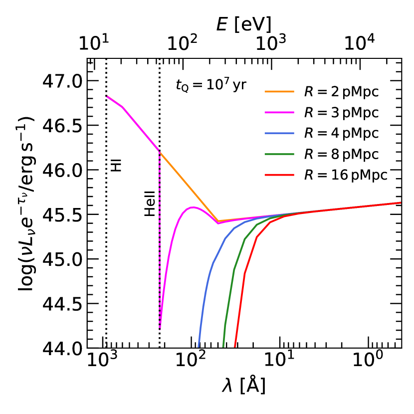
Figure 3: Ionizing spectrum (i.e. photon energies $E>13.6\rm\,eV$) at different distances from a $M_{1450}=-27$ quasar after following the radiative transfer of the intrinsic quasar SED displayed in Fig. 1 through a uniform, neutral IGM with density $\Delta=1$ at $z=7$. The spectrum corresponds to the model shown by the green curves in Fig. 2 for an optically/UV bright lifetime of $t_{\rm Q}=10^{7}\rm\,yr$. The ionization thresholds for H$\,\rm\scriptstyle I$ and He$\,\rm\scriptstyle II$ are displayed as dotted vertical lines. Note that only X-ray photons propagate unimpeded beyond the H$\,\rm\scriptstyle II$ ionization front, which is located at $R=3.5\rm\,pMpc$ in Fig. 2.

2.2 Ly$\alpha$ and 21-cm absorption in a homogeneous medium

We examine the Ly$\alpha$ and 21-cm absorption in the vicinity of bright quasars by constructing mock absorption spectra from the sight lines extracted from our RT simulations. We calculate the Ly$\alpha$ optical depth, $\tau_{\rm Ly\alpha}$, along each quasar sight line following Bolton & Haehnelt (2007) (see their eq. (15)), where we use the Tepper-García (2006) approximation for the Voigt line profile. To compute the 21-cm forest optical depth, $\tau_{21}$, we follow the approach described in Šoltinský et al. (2021) and assume a Gaussian line profile (see their eq. (9)). We shall assume strong Ly$\alpha$ coupling when calculating the 21-cm optical depths, such that the hydrogen spin temperature, $T_{\rm S}$, is equal to the gas kinetic temperature, $T$. At the redshifts ($z\leq 8$) and typical gas kinetic temperatures ($T\lesssim 10^{2}\rm\,K)$ considered in this work, the hydrogen spin temperature, $T_{\rm S}$, should be strongly coupled to the gas kinetic temperature, $T$, for reasonable assumptions regarding the Ly$\alpha$ background, even in the absence of a nearby quasar (see fig. 3 of Šoltinský et al., 2021). Although we do not model the Ly$\alpha$ photons emitted by the quasar, these would promote even stronger coupling of $T_{\rm S}$ and $T$ in the proximate gas by locally enhancing the Ly$\alpha$ background. For reference, in the absence of redshift space distortions, the optical depth to 21-cm photons at redshift $z$ is then

$$\tau_{21}(z)=0.19x_{\rm HI}\left(\frac{\Delta}{10}\right)\left(\frac{T_{\rm S}}{10\rm\,K}\right)^{-1}\left(\frac{1+z}{8}\right)^{3/2},$$ (3)

where $\Delta=\rho/\langle\rho\rangle$ is the ratio of the gas density to the mean background value, and the factor of $0.19$ is cosmology dependent (Madau et al., 1997). Strong absorption will therefore arise from dense, cold and significantly neutral hydrogen gas.

First, to develop intuition, we shall consider the propagation of ionizing radiation from a quasar into a homogeneous medium. We assume $\Delta=\rho/\langle\rho\rangle=1$, ignore peculiar velocities, and assume the gas is initially cold and neutral. Fig. 2 shows the results from an RT simulation for a quasar at $z=7$ with $M_{\rm AB}=-27$, assuming our fiducial SED. The outputs for different optically/UV bright lifetimes, $t_{\rm Q}$, for the quasar are shown by the coloured curves and are labelled in the lower left panel.

The top left panel in Fig. 2 shows the neutral hydrogen ($x_{\rm HI}$, solid curves) and singly-ionized helium ($x_{\rm HeII}$, dotted curves) fractions around the quasar. One can see the H$\,\rm\scriptstyle II$ and He$\,\rm\scriptstyle III$ ionization fronts expanding with time. The hydrogen within the quasar H$\,\rm\scriptstyle II$ region is highly ionized ($x_{\rm HI}<10^{-4}$), and the gas is optically thin to Ly$\alpha$ photons. This is demonstrated in the bottom left panel of Fig. 2 where we show the Ly$\alpha$ transmission, $F_{\rm Ly\alpha}=e^{-\tau_{\rm Ly\alpha}}$. Note, however, that the Ly$\alpha$ transmission does not saturate at the position of the H$\,\rm\scriptstyle II$ ionization front. This is particularly apparent for larger optically/UV bright lifetimes, $t_{\rm Q}>10^{7}\rm\,yr$. This is in part due to the IGM Ly$\alpha$ damping wing from the neutral IGM that is evident in the Ly$\alpha$ transmission profile (Miralda-Escudé & Rees, 1998; Mesinger & Furlanetto, 2008; Bolton et al., 2011), but also because the residual neutral hydrogen density close to the H$\,\rm\scriptstyle II$ ionization front has already risen above the threshold required for saturated Ly$\alpha$ absorption (see e.g. Bolton & Haehnelt, 2007; Lidz et al., 2007; Maselli et al., 2007; Keating et al., 2015; Eilers et al., 2017; Davies et al., 2020; Chen & Gnedin, 2021, for further details).

The gas temperature around the quasar, displayed in the top right panel of Fig. 2, is $T\sim 2$–$3\times 10^{4}\rm\,K$ behind the H$\,\rm\scriptstyle II$ and He$\,\rm\scriptstyle III$ ionization fronts (e.g. D’Aloisio et al., 2019). However, there is also heating of the neutral gas ahead of the H$\,\rm\scriptstyle II$ ionization front. For example, for $t_{\rm Q}=10^{7}\rm\,yr$ (green curve), the average gas temperature ahead of the H$\,\rm\scriptstyle II$ ionization front position at $R=3.5\rm\,pMpc$ is $\langle T\rangle\sim 100\rm\,K$. This heating is due to soft X-ray photons with long mean free paths, $\lambda_{\rm X}$, that can penetrate into the neutral IGM. For an H$\,\rm\scriptstyle I$ photo-ionization cross section $\sigma_{\rm HI}=6.34\times 10^{-18}\mathrm{\,cm^{2}}\,(E/13.6\rm\,eV)^{-2.8}$ we obtain

$$\lambda_{\rm X}=\frac{1}{n_{\rm HI}\sigma_{\rm HI}}\simeq 1.0\mathrm{\,pMpc}\,x_{\rm HI}^{-1}\Delta^{-1}\left(\frac{E}{0.2\rm\,keV}\right)^{2.8}\left(\frac{1+z}{8}\right)^{-3}.$$ (4)

The role of X-rays is further evident from Fig. 3, which shows the IGM attenuated quasar luminosity, $L_{\nu}e^{-\tau_{\nu}}$, at different distances, $R$, from the quasar assuming an optically/UV bright lifetime of $t_{\rm Q}=10^{7}\rm\,yr$ (the green curves in Fig. 2). Beyond the H$\,\rm\scriptstyle II$ ionization front (i.e. $R\geq 3.5\rm\,pMpc$) only X-ray photons penetrate into the neutral IGM surrounding the quasar H$\,\rm\scriptstyle II$ region. This long range X-ray heating acts to suppress the $21$-cm absorption from neutral gas by increasing the H$\,\rm\scriptstyle I$ spin temperature (see e.g. Xu et al., 2011; Mack & Wyithe, 2012; Šoltinský et al., 2021) and thus lowering the 21-cm optical depth. Note also that at $R=2\rm\,pMpc$ (orange curve in Fig. 3) the IGM is optically thin and the quasar spectrum matches the intrinsic SED in Fig. 1, while the spectrum at $R=3\rm\,pMpc$ (fuchsia curve) lies between the H$\,\rm\scriptstyle II$ and He$\,\rm\scriptstyle III$ ionization front and therefore exhibits a strong absorption edge at the He$\,\rm\scriptstyle II$ ionization potential, $E=54.4\rm\,eV$.

The lower right panel of Fig. 2 shows the resulting $21$-cm transmission, $F_{21}=e^{-\tau_{21}}$, around the quasar. Here $\tau_{21}\ll 1$ behind the H$\,\rm\scriptstyle II$ ionization front because the gas is hot and ionized, but where the gas (and spin) temperature decrease to $T=T_{\rm S}<100\rm\,K$, some 21-cm absorption (i.e. $F_{21}<1$) is apparent. For longer optically/UV bright lifetimes the quasar H$\,\rm\scriptstyle II$ region expands and X-ray heating extends further into the neutral IGM. The 21-cm absorption close to the quasar then becomes partially or completely suppressed even if the gas ahead of the H$\,\rm\scriptstyle II$ ionization front remains largely neutral.

In summary, we expect the Ly$\alpha$  transmission arising from the highly ionized hydrogen around quasars to be influenced by UV photons, but for neutral hydrogen, the $21$-cm forest absorption will be very sensitive to long range heating by the X-ray photons emitted by the quasar. We now turn to consider more detailed simulations of Ly$\alpha$ and $21$-cm absorption around quasars using realistic density, peculiar velocity and ionization fields extracted from the Sherwood-Relics simulations.

3 Near-zones in inhomogeneous reionization simulations

3.1 Hydrodynamical simulations

We use a subset of simulations drawn from the Sherwood-Relics project (Puchwein et al., 2022) to generate realistic Ly$\alpha$ and 21-cm forest spectra around bright quasars. The Sherwood-Relics models are high resolution cosmological hydrodynamical simulations performed with a modified version of P-Gadget-3 (Springel, 2005). These are combined with 3D RT simulations of (stellar photon driven) inhomogeneous reionization performed with the moment based, M1-closure code ATON (Aubert & Teyssier, 2008). Unlike many other radiation-hydrodynamical simulations of patchy reionization (e.g. Gnedin, 2014; Finlator et al., 2018; Ocvirk et al., 2021; Lewis et al., 2022; Garaldi et al., 2022), Sherwood-Relics uses a novel, hybrid approach for self-consistently coupling the pressure response of the gas on small scales to the inhomogeneous heating from reionization (see also Oñorbe et al., 2019). The ATON RT simulations are performed first, and the resulting three dimensional maps for the photo-ionization and photo-heating rates are then applied on-the-fly to the hydrodynamical simulations (see Puchwein et al., 2022; Gaikwad et al., 2020; Šoltinský et al., 2021; Molaro et al., 2022, for further details). The main advantage that Sherwood-Relics offers for this work is it provides a model for the spatial variations expected in the H$\,\rm\scriptstyle I$ fraction and photo-ionization rates around the dark matter haloes hosting bright quasars at $z\geq 6$ (see also Lidz et al., 2007; Satyavolu et al., 2022).

All the simulations follow $2\times 2048^{3}$ dark matter and baryon particles in a $(40h^{-1}$cMpc$)^{3}$ volume, and have a flat $\Lambda$CDM cosmology with $\Omega_{\Lambda}=0.692$, $\Omega_{\rm m}=0.308$, $\Omega_{\rm b}=0.0482$, $\sigma_{8}=0.829$, $n_{\rm s}=0.961$, $h=0.678$, consistent with Planck Collaboration (2014). The assumed primordial helium fraction by mass is $Y=0.24$ (Hsyu et al., 2020). Gas particles with density $\Delta>10^{3}$ and kinetic temperature $T<10^{5}\rm\,K$ are converted into collisionless star particles (Viel et al., 2004). Our chosen mass resolution, corresponding to a dark matter particle mass of $7.9\times 10^{5}\rm\,M_{\odot}$, is sufficient for resolving the Ly$\alpha$ forest and 21-cm absorption from the diffuse IGM (Gaikwad et al., 2020; Šoltinský et al., 2021), although note it will not resolve dark matter haloes with masses $\lesssim 2.5\times 10^{7}\rm\,M_{\odot}$.

In this work we analyse Sherwood-Relics runs that use the three reionization histories first described by Molaro et al. (2022) (see their fig. 2), in which reionization completes at $z_{\rm R}=5.3$, $z_{\rm R}=6.0$ and $z_{\rm R}=6.6$ (labelled RT-late, RT-mid and RT-early, respectively). Here we define $z_{\rm R}$ as the redshift where the volume averaged neutral fraction first falls below $\langle x_{\rm HI}\rangle\sim 10^{-3}$. The volume averaged H$\,\rm\scriptstyle I$  fractions in the simulations at $z=6,\,7$ and $8$ are listed in Table 1. All three models are consistent with existing constraints on $\langle x_{\rm HI}\rangle$ at $z>6$ and the CMB electron scattering optical depth, but the RT-late model in particular is chosen to match the $z_{\rm R}$ required by the large scale fluctuations observed in the Ly$\alpha$ forest effective optical depth at $z\gtrsim 5$ (Becker et al., 2015b; Kulkarni et al., 2019; Keating et al., 2020; Bosman et al., 2022; Zhu et al., 2022). We use RT-late for our fiducial reionization model in this work.

Table 1: The volume averaged H$\,\rm\scriptstyle I$ fraction in the IGM, $\langle x_{\rm HI}\rangle$, at redshift $z=6,\,7$ and $8$ for the three Sherwood-Relics simulations used in this work: RT-late, RT-mid and RT-early (see Molaro et al., 2022, for further details).

Model	$\langle x_{\rm HI}\rangle,\,z=6$	$\langle x_{\rm HI}\rangle,\,z=7$	$\langle x_{\rm HI}\rangle,\,z=8$
RT-late	$1.42\times 10^{-1}$	$4.75\times 10^{-1}$	$7.07\times 10^{-1}$
RT-mid	$2.39\times 10^{-3}$	$4.44\times 10^{-1}$	$7.12\times 10^{-1}$
RT-early	$7.70\times 10^{-6}$	$1.56\times 10^{-1}$	$5.49\times 10^{-1}$

In order to construct realistic quasar sight-lines from Sherwood-Relics simulations, we first use a friends-of-friends halo finder to identify dark matter haloes in the simulations. We select haloes with mass $>10^{10}\rm\,M_{\odot}$ and extract sight lines in three orthogonal directions around them. The mass of the dark matter haloes that host supermassive black holes is uncertain, although clustering analyses at lower redshift suggest $\sim 10^{12}\rm\,M_{\odot}$ (e.g. Shen et al., 2007), which is significantly larger than our minimum halo mass. However, as discussed by Keating et al. (2015) and Satyavolu et al. (2022), the choice of halo mass has a very limited impact on the sizes of quasar Ly$\alpha$ near-zones. This is because the halo bias at $\gtrsim 2\rm\,pMpc$ from a halo at $z\gtrsim 6$ is very small (see also Calverley et al., 2011; Chen et al., 2022). We have confirmed this is also true for the 21-cm absorption from the diffuse IGM we consider in this work. Next, we splice these halo sight lines (consisting of the gas overdensity $\Delta$, gas peculiar velocity $v_{\rm pec}$, gas temperature $T$, neutral hydrogen fraction $x_{\rm HI}$, and UV background photo-ionization rate $\Gamma_{\rm HI}$) with skewers drawn randomly through the simulation volume to give a total sight line length of $100h^{-1}\rm\,cMpc$. Each of the randomly drawn skewers is taken from simulation outputs sampled every $\Delta z=0.1$ to account for the redshift evolution along the quasar line of sight. Individual skewers are connected at pixels where $\Delta$, $T$, $x_{\rm HI}$ and $v_{\rm pec}$ agree within $<10$ per cent. For every model parameter variation, we then construct $2000$ unique sight lines for performing the 1D quasar RT calculations.

Finally although our hydrodynamical simulations follow heating from adiabatic compression, shocks and photo-ionization by an inhomogeneous UV radiation field, they do not model neutral gas heated and ionized by the high redshift X-ray background. We therefore follow Šoltinský et al. (2021) (see section 2.2 and appendix B in that work) and include the pre-heating of the neutral IGM by assuming a uniform X-ray background emissivity

$$\epsilon_{\rm X,\nu}(z)=~{} 3.5\times 10^{21}f_{\rm X}\rm\,erg\,s^{-1}\,Hz^{-1}\,cMpc^{-3}$$

$$\times\left(\frac{\nu}{\nu_{\rm 0.2\rm\,keV}}\right)^{-\alpha_{\rm Xb}}\left(\frac{\rho_{\rm SFR}(z)}{10^{-2}\rm\,M_{\odot}\rm\,yr^{-1}\,cMpc^{-3}}\right),$$ (5)

for photons with $E>0.2\rm\,keV$, where $f_{\rm X}$ is the uncertain X-ray efficiency (e.g. Furlanetto, 2006b), $\alpha_{\rm Xb}=1.5$ and $\rho_{\rm SFR}(z)$ is the comoving star formation rate density from Puchwein et al. (2019). We consider $0.01\leq f_{\rm X}\leq 0.1$ in this work, which is equivalent to $10^{36.2}\rm\,erg\,s^{-1}\,cMpc^{-3}\leq\epsilon_{\rm X,0.5-2\rm\,keV}\leq 10^{37.2}\rm\,erg\,s^{-1}\,cMpc^{-3}$ at $z=7$. This is consistent with the $1\sigma$ lower limit of $\epsilon_{\rm X,0.5-2\rm\,keV}\gtrsim 10^{34.5}\rm\,erg\,s^{-1}\,cMpc^{-3}$ at $6.5<z<8.7$ inferred from Murchison Widefield Array data (Greig et al., 2021).

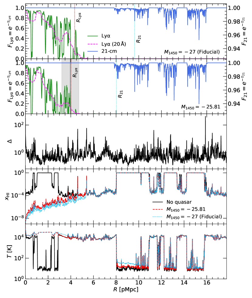
Figure 4: An example of simulated Ly$\alpha$ and 21-cm absorption in the vicinity of a bright quasar at $z=7$, obtained from the RT-late Sherwood-Relics simulation with $\langle x_{\rm HI}\rangle=0.48$ combined with a 1D RT calculation for the quasar radiation. The quasar has an optically/UV bright lifetime of $t_{\rm Q}=10^{7}\rm\,yr$ and an X-ray background efficiency of $f_{\rm X}=0.01$ is assumed. Top panel: The Ly$\alpha$ (green curves) and 21-cm (blue curves) transmission for our fiducial quasar SED with $M_{\rm 1450}=-27$. Note the scale for $F_{21}$ is shown on the right vertical axis. The dashed fuchsia curve shows the Ly$\alpha$ transmission after smoothing by a boxcar of width $20\,$\mathrm{\text{\r{A}}}$$, with the Ly$\alpha$ near-zone size, $R_{\rm Ly\alpha}$, shown by the vertical brown dotted line. The 21-cm forest spectrum is smoothed by a boxcar of width $5\rm\,kHz$ and the cyan vertical line, labelled with $R_{21}$, shows the distance from the quasar where the 21-cm absorption first reaches $F_{21}=0.99$. Second panel: As for the top panel, but for a fainter quasar absolute magnitude of $M_{1450}=-25.81$, matching the $z=6.82$ radio-loud quasar PSO J172+18 (Bañados et al., 2021). The grey band shows the observed $R_{\rm Ly\alpha}$ for PSO J172+18. Middle panel: Gas overdensity, $\Delta=\rho/\langle\rho\rangle$, along the sight line. Fourth panel: Neutral hydrogen fraction, $x_{\rm HI}$, for the case of no quasar (black curve), the fiducial quasar model (cyan dotted curve) and for the fainter quasar that mimics PSO J172$+$18 (red dashed curve). Bottom panel: Gas temperature, where the line styles match those in the panel above.

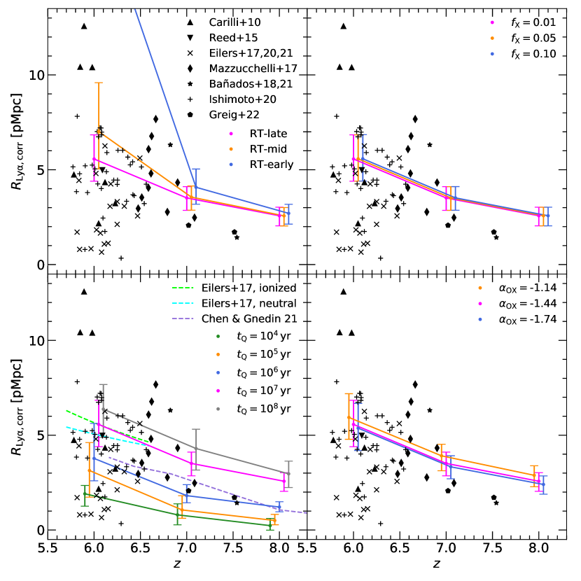
Figure 5: The redshift evolution of observed and simulated Ly$\alpha$ near-zone sizes. The filled circles at $z=6,\,7$ and $8$ connected by solid lines show the median $R_{\rm Ly\alpha}$ and $68$ per cent scatter from $2000$ simulated quasar sight lines. Clockwise from the top left, each panel shows the effect of varying one parameter around our fiducial model value: the reionization history of the Sherwood-Relics model (and hence the initial volume averaged H$\,\rm\scriptstyle I$ fraction in the IGM, see Table 1), the efficiency parameter for the X-ray background, $f_{\rm X}$, the optical-to-X-ray spectral index of the quasar, $\alpha_{\rm OX}$, and the optically/UV bright lifetime of the quasar, $t_{\rm Q}$, assuming a “light bulb” model for the quasar light curve. Note that the data point at $z=6$ for the RT-early model (blue, top left panel) is outside the range shown here. Results from the 1D RT simulations performed by Eilers et al. (2017) for an optically/UV bright lifetime of $t_{\rm Q}=10^{7.5}\rm\,yr$ are also shown for an initially highly ionized IGM (dashed green line) or fully neutral IGM (dashed cyan line) in the bottom left panel. In this panel we also show results from the 1D RT simulations from Chen & Gnedin (2021) for $t_{\rm Q}=10^{6}\rm\,yr$ and an inhomogeneously reionized IGM (dashed purple curve). The observed $R_{\rm Ly\alpha}$  (black data points, Carilli et al., 2010; Reed et al., 2015; Eilers et al., 2017; Eilers et al., 2020; Eilers et al., 2021; Mazzucchelli et al., 2017; Bañados et al., 2018, 2021; Ishimoto et al., 2020; Greig et al., 2022) have been rescaled to correspond to an absolute magnitude of $M_{1450}=-27$ (see Eq. 7).

3.2 Example Ly$\alpha$ and 21-cm absorption spectrum

A simulated quasar spectrum at $z=7$ constructed from the RT-late simulation is displayed in Fig. 4. The upper two panels show the Ly$\alpha$ (solid green curves) and 21-cm absorption (solid blue curves) for our fiducial SED with $M_{1450}=-27$, and for a fainter quasar with $M_{1450}=-25.81$, corresponding to an ionizing photon emissivity of $\dot{N}=5.48\times 10^{56}\rm\,s^{-1}$. Both models assume an optically/UV bright quasar lifetime of $t_{\rm Q}=10^{7}\rm\,yr$ and an X-ray background efficiency $f_{\rm X}=0.01$. The fainter absolute magnitude is chosen to match the radio-loud quasar PSO J172$+$18 at $z=6.82$, recently presented by Bañados et al. (2021). The lower three panels display the gas overdensity, $\Delta=\rho/\langle\rho\rangle$, neutral hydrogen fraction, $x_{\rm HI}$, and gas temperature, $T$, for the case of no quasar (black curves), the fiducial quasar model (cyan dotted curves) and for the fainter quasar that mimics PSO J172$+$18 (red dashed curves). Note the pre-existing neutral and ionized regions associated with patchy reionization, and the heating of neutral gas ahead of the large ionized region at $R>8\rm\,pMpc$ by the X-ray emission from the quasar. The 21-cm absorption is only present where the gas is neutral, and it is stronger for the $M_{1450}=-25.81$ quasar due to the lower gas (and H$\,\rm\scriptstyle I$ spin) temperature at $R>8\rm\,pMpc$. There is also a proximate Lyman limit system at $R\sim 5.4\rm\,pMpc$ that terminates the quasar H$\,\rm\scriptstyle II$ ionization front, beyond which the neutral hydrogen fractions are very similar for all the three cases (see also Chen & Gnedin, 2021).

We obtain the size of the simulated Ly$\alpha$ near-zones, $R_{\rm Ly\alpha}$, following the definition introduced by Fan et al. (2006). This is the point where the normalised transmission first drops below $F_{\rm Ly\alpha}=0.1$ after smoothing the Ly$\alpha$ spectrum with a boxcar of width $20\,$\mathrm{\text{\r{A}}}$$. The smoothed spectrum is shown by the fuchsia dashed curves in the upper panels of Fig. 4. For our fiducial quasar SED we obtain $R_{\rm Ly\alpha}=4.34\rm\,pMpc$ (shown by the vertical brown dotted line in Fig. 4), and for the fainter quasar with $M_{1450}=-25.81$ we find $R_{\rm Ly\alpha}=4.03\rm\,pMpc$. In this case we have deliberately chosen a simulated quasar sight line that matches the observed Ly$\alpha$ near-zone size of $R_{\rm Ly\alpha}$ $=3.96\pm 0.48\rm\,pMpc$ for PSO J172+18 (Bañados et al., 2021), shown by the grey band in the second panel of Fig. 4. As noted by Bañados et al. (2021), after correcting for the quasar luminosity, the Ly$\alpha$ near-zone size for PSO J172+18 is in the top quintile of $R_{\rm Ly\alpha}$ for quasars at $z\gtrsim 6$. Our modelling suggests a possible explanation is that PSO J172+18 is surrounded by an IGM that is (locally) highly ionized due to UV emission from galaxies, despite the average H$\,\rm\scriptstyle I$ fraction in the IGM being much larger. For example, for the model displayed in Fig. 4, the average IGM neutral fraction is $\langle x_{\rm HI}\rangle=0.48$, but there is a pre-existing highly ionized region with $x_{\rm HI}\sim 10^{-4}$ close to the quasar halo at $R\sim 3$–$8\rm\,pMpc$.

In Fig. 4 we have also marked the distance from the quasar, $R_{21}$, where the proximate 21-cm absorption first reaches a threshold of $F_{21,\rm th}=e^{-\tau_{21}}=0.99$ after smoothing the spectrum with a boxcar of width $5\rm\,kHz$ (vertical cyan dotted lines). This occurs at $R_{21}=9.63\rm\,pMpc$ ($R_{21}=8.03\rm\,pMpc$) for the $M_{\rm AB}=-27$ ($M_{\rm AB}=-25.81$) quasar. In what follows, we will use this as our working definition of what we term the “21-cm near-zone” size, although we discuss this choice further in Appendix A. Note that – in analogy to the Ly$\alpha$ near-zone – because of X-ray heating beyond the ionization front and the patchy ionization state of the IGM, $R_{21}$ does not always correspond to the position of the quasar H$\,\rm\scriptstyle II$ ionization front. We find that when averaging over $2000$ sight-lines $R_{21}$ does, however, scale with the quasar ionizing photon emission rate as $R_{21}\propto\dot{N}^{1/3}$. This is the same scaling expected for the size of the quasar H$\,\rm\scriptstyle II$ region (see Appendix B for details).

Lastly, given our definition for $R_{21}$, we may also estimate the minimum radio source flux density, $S_{\rm min}$, required to detect an absorption feature with $F_{21,\rm th}=0.99$ for a signal-to-noise ratio, $\rm S/N$. Using eq. (13) in Šoltinský et al. (2021) and adopting values representative for SKA1-low (Braun et al., 2019), we find

$$S_{\rm min}=~{} 17.2\rm\,mJy\left(\frac{0.01}{1-\textit{F}_{21,\rm th}}\right)\left(\frac{\rm S/N}{5}\right)\left(\frac{5\rm\,kHz}{\Delta\nu}\right)^{1/2}\left(\frac{1000\rm\,hr}{\textit{t}_{\rm int}}\right)^{1/2}$$

$$\times\left(\frac{600\rm\,m^{2}\,K^{-1}}{A_{\rm eff}/T_{\rm sys}}\right),$$ (6)

where $T_{\rm sys}$ is the system temperature, $\Delta\nu$ is the bandwidth, $A_{\rm eff}$ is the effective area of the telescope and $t_{\rm int}$ is the integration time. For a sensitivity appropriate for SKA1-low (SKA2), $A_{\rm eff}/T_{\rm sys}\simeq 600\rm\,m^{2}\,K^{-1}$ ($5500\rm\,m^{2}\,K^{-1}$) (Braun et al., 2019), an integration time of $t_{\rm int}=1000\rm\,hr$ ($100\rm\,hr$) and $\rm S/N=5$, we obtain $S_{\rm min}=17.2\rm\,mJy$ ($5.9\rm\,mJy$). For comparison, PSO J172+18 has a $3\sigma$ upper limit on the flux density at $147.5\rm\,MHz$ of $S_{147.5\rm\,MHz}<8.5\rm\,mJy$ (Bañados et al., 2021). The brightest known radio-loud blazar at $z>6$, PSO J0309+27 at $z=6.1$ with $M_{\rm 1450}=-25.1$, instead has a flux density $S_{147\rm\,MHz}=64.2\pm 6.2\rm\,mJy$ (Belladitta et al., 2020). Both objects are therefore potential targets for detecting proximate 21-cm absorption from the diffuse IGM, although note the shape of their SEDs will be rather different.

3.3 Comparison to observed Ly$\alpha$ near-zone sizes

Next, as a consistency check of our model, we compare the Ly$\alpha$ near-zone sizes predicted in our simulations to the observed distribution in Fig. 5. We have compiled a sample of Ly$\alpha$ near-zone sizes measured from the spectra of 76 $z>5.77$ quasars (Carilli et al., 2010; Reed et al., 2015; Eilers et al., 2017; Eilers et al., 2020; Eilers et al., 2021; Mazzucchelli et al., 2017; Bañados et al., 2018, 2021; Ishimoto et al., 2020; Greig et al., 2022). We use the (model dependent) $R_{\rm Ly\alpha}$–$M_{1450}$ scaling relation derived by Eilers et al. (2017) to approximately correct for differences in the quasar absolute magnitudes. For an observed absolute magnitude of $M_{\rm 1450,obs}$, this gives a corrected Ly$\alpha$ near-zone size of

$$R_{\rm Ly\alpha,corr}=R_{\rm Ly\alpha,obs}\times 10^{0.4\left(27+M_{\rm 1450,obs}\right)/2.35}\propto\dot{N}^{0.43}.$$ (7)

In this work we rescale the observed sizes, $R_{\rm Ly\alpha,obs}$, to obtain a corrected size, $R_{\rm Ly\alpha,corr}$, at our fiducial absolute magnitude $M_{1450}=-27$.

In each panel of Fig. 5 we vary one parameter around our fiducial model values and compare the simulated Ly$\alpha$ near-zone sizes at $z=6,\,7$ and $8$ to the observed $R_{\rm Ly\alpha,corr}$. Clockwise from the upper left, the parameters varied are: the reionization history of the Sherwood-Relics model (and hence the initial volume averaged H$\,\rm\scriptstyle I$ fraction in the IGM, see Table 1), the efficiency parameter for the X-ray background, $f_{\rm X}$, the optical-to-X-ray spectral index of the quasar, $\alpha_{\rm OX}$, and the optically/UV bright lifetime of the quasar, $t_{\rm Q}$, assuming a “light bulb" model for the quasar light curve. At each redshift, we show the median $R_{\rm Ly\alpha}$ and the $68$ per cent distribution from $2000$ simulated sight lines. For comparison, in the lower left panel we also show the results from the 1D RT simulations performed by Eilers et al. (2017) for an optically/UV bright lifetime of $t_{\rm Q}=10^{7.5}\rm\,yr$, assuming either a highly ionized IGM (dashed green line) or fully neutral IGM (dashed cyan line). The results for our fiducial parameters (i.e. RT-late, $f_{\rm X}=0.01$, $\alpha_{\rm OX}=-1.44$ and $t_{\rm Q}=10^{7}\rm\,yr$) are consistent with the Eilers et al. (2017) models within the $68$ per cent scatter. Similarly, the dashed purple curve shows the 1D RT simulations from Chen & Gnedin (2021) for $t_{\rm Q}=10^{6}\rm\,yr$, which – allowing for the somewhat larger $\langle x_{\rm HI}\rangle$ we have assumed in the RT-late reionization model – are again similar to this work if using the same optically/UV bright quasar lifetime.

In general, the simulated $R_{\rm Ly\alpha}$ decreases with increasing redshift (e.g. Fan et al., 2006; Wyithe, 2008; Carilli et al., 2010) and, as shown in the upper left panel of Fig. 5, models with a larger initial IGM H$\,\rm\scriptstyle I$ fraction produce slightly smaller Ly$\alpha$ near-zone sizes. Note, however, that any inferences regarding $\langle x_{\rm HI}\rangle$ from $R_{\rm Ly\alpha}$ will be correlated with the assumed optically/UV bright lifetime (e.g. Bolton et al., 2011; Keating et al., 2015). Furthermore, at $z=6$ the $R_{\rm Ly\alpha}$ for RT-early (blue data points), which has a volume averaged H$\,\rm\scriptstyle I$ fraction of $\langle x_{\rm HI}\rangle=7.7\times 10^{-6}$ at this redshift, is outside the range displayed. This is because many sight lines in this model are highly ionized and do not have ($20\,$\mathrm{\text{\r{A}}}$$ smoothed) Ly$\alpha$ transmission that falls below $F_{\rm Ly\alpha}=0.1$. For RT-early at $z=6$, we instead obtain a $68$ per cent lower limit of $R_{\rm Ly\alpha}>18.33\rm\,pMpc$, suggesting that the UV background at $z\simeq 6$ is significantly overproduced by the RT-early model. In contrast, varying the X-ray heating of the IGM, either by changing $f_{\rm X}$ or $\alpha_{\rm OX}$ (upper and lower right panels, respectively), has very little effect on the Ly$\alpha$ near-zone sizes. As already discussed in Section 2.2, this is because the ionization and heating by X-rays is important only for the cold, neutral IGM, and not the ionized gas observed in Ly$\alpha$ transmission.

Finally, in the lower left panel of Fig. 5, we observe that some of the scatter in the observational data may be reproduced by varying the optically/UV bright lifetime of the quasar. Indeed, Morey et al. (2021) have recently demonstrated that the majority of $R_{\rm Ly\alpha,\rm corr}$ measurements at $z\simeq 6$ are reproduced assuming a median optically/UV bright lifetime of $t_{\rm Q}=10^{5.7}\rm\,yr$ with a $95$ per cent confidence interval $t_{\rm Q}=10^{5.3}$–$10^{6.5}\rm\,yr$. We have independently checked this with our own modelling and found broadly similar results (see Appendix C), although there is a hint that slightly larger quasar lifetimes may be favoured within our late reionization model (see also Satyavolu et al., 2022). On the other hand, the largest Ly$\alpha$ near-zones with $R_{\rm Ly\alpha,corr}\geq 10\rm\,pMpc$ reported by Carilli et al. (2010) are not reproduced by the RT-late simulation even for $t_{\rm Q}=10^{8}\rm\,yr$, suggesting the IGM along these sight lines may be more ionized than assumed in the RT-late model. It is also possible our small box size of $40h^{-1}\rm\,cMpc$ fails to correctly capture large ionized regions near the quasar host haloes at the tail-end of reionization (cf. Iliev et al., 2014; Kaur et al., 2020), and may therefore miss sight lines with the largest $R_{\rm Ly\alpha}$. Of particular interest here, however, are the quasars with $R_{\rm Ly\alpha,corr}\lesssim 2\rm\,pMpc$ (Eilers et al., 2020; Eilers et al., 2021), which correspond to $\lesssim 10$ per cent of the observational data at $z\simeq 6$. As noted by Eilers et al. (2021), a very short optically/UV bright quasar lifetime of $t_{\rm Q}\lesssim 10^{4}$–$10^{5}\rm\,yr$ is required to reproduce these Ly$\alpha$ near-zone sizes. The implied average optically/UV bright lifetime of $t_{\rm Q}\sim 10^{6}\rm\,yr$, consistent with Morey et al. (2021), therefore presents an apparent challenge for black hole growth at $z\geq 6$. We discuss this further in Section 5.1.

In summary, the Ly$\alpha$ forest near-zone sizes predicted by our simulations assuming a late end to reionization at $z\simeq 5.3$ are consistent with both independent modelling and the observational data if we allow for a distribution of optically/UV bright quasar lifetimes (e.g. Morey et al., 2021). We now use this model to explore the expected proximate 21-cm forest absorption around (radio-loud) quasars at $z\geq 6$.

4 Predicted extent of proximate 21-cm absorption

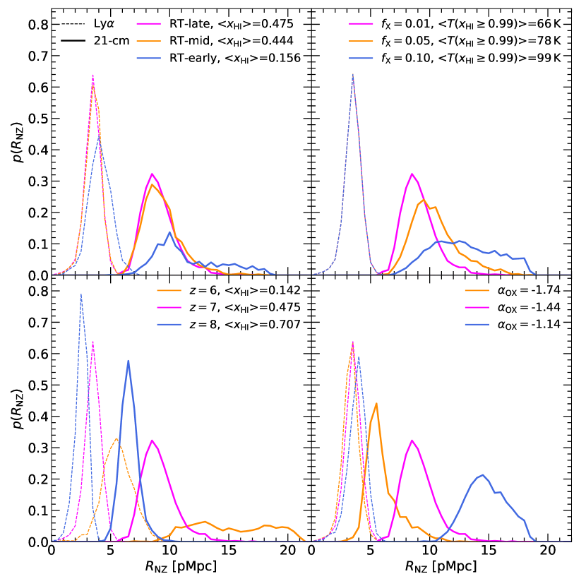
Figure 6: Probability distributions for Ly$\alpha$ (dashed thin curves) and 21-cm (solid thick curves) near-zone sizes obtained from $2000$ simulated quasar sight lines (see Section 3.2 for the definition of $R_{\rm Ly\alpha}$ and $R_{21}$). The distributions show the effect of varying parameters around our fiducial model. Clockwise from the top left, these parameters are: the reionization history, the X-ray background efficiency $f_{\rm X}$, the quasar optical-to-X-ray spectral index $\alpha_{\rm OX}$, and the redshift of the quasar. We also list the mean neutral hydrogen fraction (left panels) and the mean temperature in pixels with $x_{\rm HI}\geq 0.99$ (top right panel) prior to any quasar heating. The fiducial values at $z=7$ are RT-late with $\langle x_{\rm HI}\rangle=0.48$, $f_{\rm X}=0.01$ and $\alpha_{\rm OX}=-1.44$. All models furthermore assume an absolute magnitude of $M_{1450}=-27$ and an optically/UV bright lifetime of $t_{\rm Q}=10^{7}\rm\,yr$. Note that while $R_{\rm Ly\alpha}$ is insensitive to $f_{\rm X}$ or $\alpha_{\rm OX}$, $R_{21}$ has a strong dependence on the X-ray heating around the quasar. Both $R_{\rm Ly\alpha}$ and $R_{21}$ are sensitive to the IGM neutral fraction.

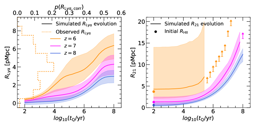
Figure 7: The dependence of the Ly$\alpha$ (left panel) and 21-cm (right panel) near-zone sizes on the optically/UV bright quasar lifetime, $t_{\rm Q}$, at $z=6$ (orange), $z=7$ (fuchsia) and $z=8$ (blue). Note the different scales on the vertical axes of the panels. The curves show the median value obtained from 2000 mock spectra, while the shaded regions mark the $68$ per cent range around the median. Upward pointing arrows give the lower 68 per cent bound on $R_{21}$ in the cases where some of the sight-lines have no pixels with $F_{21}<0.99$. The dotted orange histogram in the left panel shows the observed distribution of $R_{\rm Ly\alpha,corr}$, with a mean quasar redshift of $z=6.26$. The filled circles at $t_{\rm Q}=10^{2}\rm\,yr$ in the right panel show the median size, $R_{\rm HII}$, of the pre-existing H$\,\rm\scriptstyle II$ region surrounding the quasar host halo. All models are drawn from the RT-late simulation and assume $M_{1450}=-27$, $f_{\rm X}=0.01$ and $\alpha_{\rm OX}=-1.44$.

4.1 The effect of X-ray heating and IGM neutral fraction

The effect of X-ray heating and the IGM neutral fraction on the distribution of “21-cm near zone” sizes, $R_{21}$, predicted by our simulations is displayed in Fig. 6 (solid curves). In all cases we assume $M_{1450}=-27$ and a light bulb quasar model with an optically/UV bright lifetime of $t_{\rm Q}=10^{7}\rm\,yr$. For comparison, the $R_{\rm Ly\alpha}$ distributions from the same models are given by the dashed curves. The top left panel shows the effect of varying the reionization model, and hence the initial volume averaged neutral fraction in the IGM, $\langle x_{\rm HI}\rangle$. At $z=7$, the $\langle x_{\rm HI}\rangle$ values for RT-late (fuchsia curves) and RT-mid (orange curves) are very similar, and we find little difference between these models for $R_{21}$ or $R_{\rm Ly\alpha}$. For the more highly ionized RT-early simulation, the near-zone sizes are slightly larger, although note almost half of the $2000$ quasar spectra do not have any pixels with $F_{21}<0.99$ at $z=7$. In the bottom left panel, we instead show results from the RT-late simulation at three different redshifts, $z=6,\,7$ and $8$. The Ly$\alpha$ and 21-cm near-zone sizes are larger toward lower redshift, again due to the smaller H$\,\rm\scriptstyle I$ fraction in the IGM, but also now because of the decrease in the proper gas density (i.e. $n_{\rm H}\propto(1+z)^{3}$). However, once again, at $z=6$ (fuchsia curves) around half the quasar sight-lines do not exhibit 21-cm absorption with $F_{21}<0.99$. This suggests that observing 21-cm absorption from the diffuse IGM in close proximity to radio-loud quasars will be more likely if reionization is late ($z_{\rm R}\simeq 5.3$) as suggested by Kulkarni et al. (2019), and if suitably bright radio-loud quasars can be identified at $z\gtrsim 7$.

The effect of X-ray heating on the near-zone sizes is displayed in the right panels of Fig. 6. The top right panel shows the heating by the X-ray background, while the bottom right panel shows the effect of quasar X-ray heating when varying the optical-to-X-ray spectral index, $\alpha_{\rm OX}$. As noted earlier, $R_{\rm Ly\alpha}$ is insensitive to $f_{\rm X}$ and $\alpha_{\rm OX}$, but $R_{21}$ is sensitive to both; the average 21-cm near-zone size increases as the spin temperature of the neutral gas is raised by X-ray photo-heating. For example, for $f_{\rm X}=0.01$ the average temperature of hydrogen with $x_{\rm HI}>0.99$ (i.e. neutral gas ahead of the H$\,\rm\scriptstyle II$ ionization front) is $T=66\rm\,K$, but this increases to $T=99\rm\,K$ for $f_{\rm X}=0.1$. Here, the average temperature of neutral gas is consistent with the recent constraint of $15.6\mathrm{\,K}<T_{\rm S}<656.7\rm\,K$ (95 per cent confidence) from The HERA Collaboration (2022) in all three cases. For $T\gg 10^{2}\rm\,K$ (or equivalently, $f_{\rm X}\gg 0.1$), we expect very little 21-cm absorption will be detectable at all (e.g. Šoltinský et al., 2021). A similar situation holds for $\alpha_{\rm OX}$, with a harder quasar X-ray spectrum producing larger $R_{21}$.. Deep X-ray observations may be used to constrain $\alpha_{\rm OX}$ for at least some $z\gtrsim 6$ radio-loud quasars (Connor et al., 2021). Prior knowledge of the quasar X-ray spectrum could therefore help break some of the degeneracy between $R_{21}$ and the X-ray heating parameters $f_{\rm X}$ and $\alpha_{\rm OX}$. As already discussed, however, the location of the expanding quasar H$\,\rm\scriptstyle II$ region and the spin temperature beyond the H$\,\rm\scriptstyle II$ ionization front determine the optical depth of neutral gas, where $\tau_{21}\propto x_{\rm HI}/T_{\rm S}\sim T_{\rm S}^{-1}$. This means $R_{21}$ is also sensitive to the optically/UV bright lifetime of the quasar, $t_{\rm Q}$.

4.2 The effect of the optically/UV bright lifetime

In Fig. 7, for our fiducial model we examine how $R_{\rm Ly\alpha}$ and $R_{21}$ evolve with the optically/UV bright lifetime of the quasar at redshift $z=6$ (orange curves), $z=7$ (fuchsia curves) and $z=8$ (blue curves). The shaded regions bound $68$ per cent of the data around the median for $2000$ simulated sight-lines. The behaviour of $R_{\rm Ly\alpha}$ at $z=6$, displayed in the left panel, is qualitatively similar to the results of other recent work (e.g. Eilers et al., 2018; Eilers et al., 2021; Davies et al., 2020; Satyavolu et al., 2022). There are three distinct phases in the evolution of $R_{\rm Ly\alpha}$ at $z=6$. For a highly ionized IGM, when the optically/UV bright lifetime of the quasar is shorter than the equilibriation timescale, $t_{\rm Q}<t_{\rm eq}$, we expect $R_{\rm Ly\alpha}$ to increase with $t_{\rm Q}$. The equilibriation timescale is approximately

$$t_{\rm eq}=\frac{x_{\rm HI,\rm\,eq}}{n_{\rm e}\alpha_{A}(T)}\simeq\frac{10^{5.0}\rm\,yr}{\Delta}\left(\frac{x_{\rm HI,\rm\,eq}}{10^{-4}}\right)\left(\frac{T}{10^{4}\rm\,K}\right)^{0.72}\left(\frac{1+z}{7}\right)^{-3},$$ (8)

where $x_{\rm HI,\,eq}$ is the H$\,\rm\scriptstyle I$ fraction in ionization equilibrium, we have used a case-A recombination coefficient $\alpha_{\rm A}=4.06\times 10^{-13}\mathrm{\,cm^{3}\,s^{-1}}(T/10^{4}\rm\,K)^{-0.72}$ and assumed $n_{\rm e}=1.158n_{\rm H}$ for a fully ionized hydrogen and helium IGM. For $t_{\rm Q}>t_{\rm eq}$, the growth of the Ly$\alpha$ near-zone size slows and becomes largely insensitive to $t_{\rm Q}$ (see e.g. Bolton & Haehnelt, 2007). In this regime the near-zone size is set by the Ly$\alpha$ absorption from the residual H$\,\rm\scriptstyle I$ in the IGM, rather than the growth of the H$\,\rm\scriptstyle II$ region around the quasar. Finally, at $t_{\rm Q}\gtrsim 10^{6.5}\rm\,yr$, the Ly$\alpha$ near-zone starts to grow again. As noted by Eilers et al. (2018), the late growth of $R_{\rm Ly\alpha}$ is due to the propagation of the He$\,\rm\scriptstyle III$ ionization front into the IGM. The associated He$\,\rm\scriptstyle II$ photo-heating raises the IGM temperature and hence further lowers the H$\,\rm\scriptstyle I$ fraction in the IGM (see also Bolton et al., 2012). We also point out that the median $R_{\rm Ly\alpha}$ we obtain at $z=6$ for $10^{5}\mathrm{\,yr}<t_{\rm Q}<10^{6.5}\rm\,yr$ are slightly smaller than those reported in fig. 2 of Davies et al. (2020). This is because we use our RT-late simulation with $\langle x_{\rm HI}\rangle=0.14$ at $z=6$, instead of assuming a highly ionized IGM as Davies et al. (2020) do. In the RT-late model, neutral islands will persist in underdense regions at $z=6$ and hence slow the growth of the near-zones. Further discussion of this point can also be found in Satyavolu et al. (2022).

For reference, we also show the distribution of observed $R_{\rm Ly\alpha,corr}$ in the left panel of Fig. 7, which has a mean quasar redshift of $z=6.26$. Once again, note that reproducing the Ly$\alpha$ near-zones with $R_{\rm Ly\alpha,corr}<2\rm\,pMpc$ at $z\simeq 6$ requires $t_{\rm Q}\lesssim 10^{4}$–$10^{5}\rm\,yr$. As expected, at $z=7$ and $z=8$, the Ly$\alpha$ near-zones are smaller. Here the initial H$\,\rm\scriptstyle I$ fractions in the IGM for RT-late are $\langle x_{\rm HI}\rangle=0.48$ and $\langle x_{\rm HI}\rangle=0.71$, respectively. The large IGM H$\,\rm\scriptstyle I$ fractions also produce a strong Ly$\alpha$ damping wing that suppresses Ly$\alpha$ near-zone sizes. For reference, the $z=7.54$ quasar ULAS J1342+0928 has $R_{\rm Ly\alpha,corr}=1.43\rm\,pMpc$ (Bañados et al., 2018), whereas the $z=7.08$ quasar ULAS J1120$+$0641 has $R_{\rm Ly\alpha,corr}=2.48\pm 0.2\rm\,pMpc$ (Mortlock et al., 2011; Mazzucchelli et al., 2017). We find our simulations are consistent with these sizes for optically/UV bright lifetimes in the range $10^{4}\mathrm{\,yr}\leq t_{\rm Q}\leq 10^{6.8}\rm\,yr$.

In the right panel of Fig. 7 we show the dependence of the 21-cm near-zone size on the optically/UV bright lifetime, $t_{\rm Q}$. Note in particular the filled circles in Fig. 7 at $t_{\rm Q}=10^{2}\rm\,yr$, which show the median size, $R_{\rm HII}$, of the pre-existing H$\,\rm\scriptstyle II$ regions created by the galaxies surrounding the quasar host haloes. The initial value of $R_{21}$ is very similar to $R_{\rm HII}$, suggesting the typical size of these pre-existing H$\,\rm\scriptstyle II$ regions will set the 21-cm near-zone sizes for short optically/UV bright lifetimes. We find $R_{21}\sim R_{\rm HII}$ for $t_{\rm Q}\lesssim 10^{4}\rm\,yr$. However, for $t_{\rm Q}\gtrsim 10^{4}\rm\,yr$ (i.e. exceeding the local photo-ionization timescale at $R_{\rm HII}$, where $t_{\rm ion}=\Gamma_{\rm HI}^{-1}\sim 10^{4}$–$10^{5}\rm\,yr$), the quasar starts to expand the pre-existing H$\,\rm\scriptstyle II$ region and X-rays begin to photo-heat the neutral gas ahead of the quasar H$\,\rm\scriptstyle II$ ionization front to $T>10^{2}\rm\,K$. The 21-cm near-zone then grows. Note also that at $z=6$, there is a large $68$ per cent scatter around the median $R_{21}$, and for $t_{\rm Q}>10^{5.5}\rm\,yr$, many of the simulated sight-lines at $z=6$ have no pixels with $F_{21}<0.99$. In this case we instead show lower limits for $R_{21}$ that bound $68$ per cent of the simulated sight-lines. At $z=7$ and $z=8$, the median $R_{21}$ is smaller with significantly less scatter, which (as for the case for the Ly$\alpha$ near-zones) is primarily because the average H$\,\rm\scriptstyle I$ fraction in the IGM is larger at these redshifts.

In summary, our results suggest two intriguing possibilities. First, if there is a population of very young quasars at $z\geq 6$, as observed Ly$\alpha$ near-zones with $R_{\rm Ly\alpha}<2\rm\,pMpc$ imply (e.g. Eilers et al., 2017), then if $f_{\rm X}\lesssim 0.01$, a measurement of $R_{21}$ around these objects should constrain the size of the H$\,\rm\scriptstyle II$ region created by the galaxies clustered around the quasar host halo. Such a measurement would be complimentary to similar proposed measurements of $R_{\rm HII}$ from 21-cm tomography (e.g. Furlanetto et al., 2004; Wyithe & Loeb, 2004b; Geil & Wyithe, 2008; Datta et al., 2012; Kakiichi et al., 2017; Ma et al., 2020; Davies et al., 2021), and would provide a strong constraint on the reionization sources. Second, once the quasar begins to heat the IGM ahead of the H$\,\rm\scriptstyle II$ ionization front to $T\gtrsim 10^{2}\rm\,K$, the 21-cm absorption is suppressed and $R_{21}$ increases monotonically. In the absence of significant ionization, the cooling timescale for this gas is the adiabatic cooling timescale, where

$$t_{\rm ad}=\frac{1}{2H(z)}\simeq 10^{8.8}\mathrm{\,yr}\,\left(\frac{1+z}{8}\right)^{-3/2},$$ (9)

and $H(z)\simeq H_{0}\Omega_{\rm m}^{1/2}(1+z)^{3/2}$ is the Hubble parameter. Hence, in general $R_{21}$ should always increase and it will be sensitive to the integrated lifetime of the quasar, because we typically expect $t_{\rm Q}\lesssim t_{\rm ad}$ (e.g Haehnelt et al., 1998; Yu & Tremaine, 2002; Martini, 2004). We now turn to explore the consequence of this for variable quasar emission, with particular emphasis on the possible implications for black hole growth at $z\gtrsim 6$ (cf. Eilers et al., 2018; Eilers et al., 2021).

5 Probing integrated quasar lifetimes with proximate 21-cm absorption

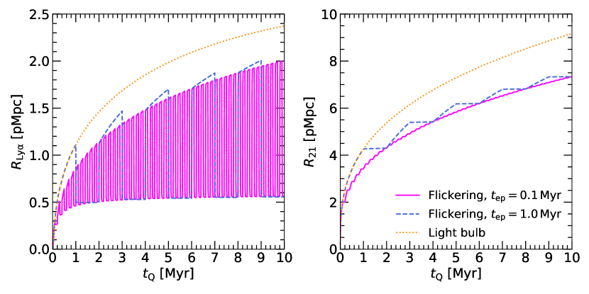
Figure 8: The dependence of $R_{\rm Ly\alpha}$ (left panel) and $R_{21}$ (right panel) on the integrated quasar lifetime, $t_{\rm Q}$, for a quasar at $z=7$ that varies between a bright phase with $M_{1450}=-27$ and faint phase with $M_{1450}=-23$. We assume an optically/UV bright duty cycle of $f_{\rm duty}=0.5$ and consider episodic lifetimes of $t_{\rm ep}=10^{5}\rm\,yr$ (fuchsia solid curves) and $t_{\rm ep}=10^{6}\rm\,yr$ (blue dashed curves). The IGM surrounding the quasar is initially cold and neutral. The near-zone size for a light bulb quasar emission model (dotted orange curves) is shown for comparison. Note in particular that while $R_{\rm Ly\alpha}$ decreases on the equilibriation timescale during the faint phase, $t_{\rm eq}$, $R_{21}$ remains almost constant due to the much longer adiabatic cooling timescale for the neutral gas, where the 21-cm optical depth $\tau_{21}\propto x_{\rm HI}/T_{\rm S}$.

5.1 A simple model for flickering quasar emission

Morey et al. (2021) have recently pointed out that the typical optically/UV bright lifetime of $t_{\rm Q}\sim 10^{6}\rm\,yr$ implied by the observed $R_{\rm Ly\alpha}$ is a challenge for the growth of $\sim 10^{9}\rm\,M_{\odot}$ black holes observed at $z\gtrsim 6$ (Mortlock et al., 2011; Bañados et al., 2018; Yang et al., 2020a; Wang et al., 2020; Farina et al., 2022). Further discussion of this point in the context of Ly$\alpha$ near-zones can be found in Eilers et al. (2018) and Eilers et al. (2021), but we briefly repeat the argument here. For a quasar with bolometric luminosity $L$, the Salpeter (1964) (or e-folding) timescale if the black hole is accreting at the Eddington limit is

$$t_{\rm S}=\frac{\epsilon}{1-\eta}\frac{c\sigma_{\rm T}}{4\pi G\mu m_{\rm p}}=4.33\times 10^{7}\mathrm{\,yr}\,\left(\frac{L}{L_{\rm E}}\right)^{-1}\left(\frac{\epsilon}{0.1}\right)\left(\frac{1-\eta}{0.9}\right)^{-1},$$ (10)

where $L_{\rm E}$ is the Eddington luminosity, $\sigma_{\rm T}$ is the Thomson cross-section, $\mu=1.158$ is the mean molecular weight for fully ionized hydrogen and helium with $Y=0.24$, $\eta$ is the accretion efficiency, and $\epsilon$ is the radiative efficiency (e.g. Shakura & Sunyaev, 1973) where we assume $\epsilon=\eta$. For a black hole seed of mass $M_{\rm seed}$ and a constant accretion rate, the black hole mass, $M_{\rm BH}$, after $t_{\rm Q}=[10^{6},\,10^{7},\,10^{8}]\rm\,yr$ is then

$$M_{\rm BH}=M_{\rm seed}\exp\left(\frac{t_{\rm Q}}{t_{\rm S}}\right)=[1.0,\,1.3,\,10.1]M_{\rm seed}.$$ (11)

If $t_{\rm Q}\sim 10^{6}\rm\,yr$ there is insufficient time for the black hole to grow; Eq. (11) requires $M_{\rm BH}\sim M_{\rm seed}\sim 10^{9}\rm\,M_{\odot}$ , yet the largest theoretically plausible seed mass is $M_{\rm seed}\sim 10^{5}$–$10^{6}\rm\,M_{\odot}$ (e.g. from the direct collapse of atomically cooled halo gas, Loeb & Rasio, 1994; Dijkstra et al., 2008; Regan et al., 2017; Inayoshi et al., 2020).

As discussed by Eilers et al. (2021), there are two possible solutions to this apparent dilemma; the $z\gtrsim 6$ quasars are indeed very young and have grown rapidly from massive seeds by radiatively inefficient ($\epsilon\sim 0.01$), mildly super-Eddington accretion (e.g. Madau et al., 2014; Volonteri et al., 2015; Davies et al., 2019) or the quasars are much older than the $R_{\rm Ly\alpha}$ measurements imply, such that $t_{\rm Q}\gtrsim 10^{7}\rm\,yr$. This is possible if the black holes have grown primarily in an optically/UV obscured phase and the quasars have only recently started to ionize their vicinity, perhaps due to the evacuation of obscuring material by feedback processes (Hopkins et al., 2005). Alternatively, quasar luminosity may vary between optically/UV bright and faint phases over an episodic lifetime of $t_{\rm ep}\sim 10^{4}$–$10^{6}\rm\,yr$, likely as a result of variable accretion onto the black hole (Schawinski et al., 2015; King & Nixon, 2015; Anglés-Alcázar et al., 2017; Shen, 2021). In this scenario, when the quasars are faint the ionized hydrogen in their vicinity recombines on the equilibriation timescale (see Eq. 8). This produces an initially small Ly$\alpha$ near-zone size that regrows over a timescale $t_{\rm ion}=\Gamma_{\rm HI}^{-1}\sim 10^{4}$–$10^{5}\rm\,yr$ once the quasars re-enter the optically/UV bright phase (Davies et al., 2020; Satyavolu et al., 2022). Furthermore, for $t_{\rm ep}\lesssim t_{\rm eq}$ the H$\,\rm\scriptstyle I$ surrounding the quasars never fully equilibriates, and $R_{\rm Ly\alpha}$ remains smaller than predicted for a light bulb light curve with the same integrated quasar lifetime.

However, it is difficult to distinguish between these possibilities using $R_{\rm Ly\alpha}$ alone. We suggest the proximate 21-cm absorption around sufficiently radio-bright quasars may provide some further insight. The long adiabatic cooling timescale for neutral gas in the IGM means that, unlike $R_{\rm Ly\alpha}$, $R_{21}$ will be sensitive to the integrated lifetime of the quasars. To illustrate this point further consider Fig. 8, where we use the simplified neutral, homogeneous IGM model discussed in Section 2.2 and Fig. 2 to explore the effect of variable quasar emission on the evolution of $R_{\rm Ly\alpha}$ (left panel) and $R_{21}$ (right panel). In both panels the orange dotted curves show $R_{\rm Ly\alpha}$ and $R_{21}$ for a light bulb emission model with $M_{1450}=-27$ and the fiducial SED. For the variable emission model, we instead follow a similar approach to Davies et al. (2020) and Satyavolu et al. (2022) and assume the quasar periodically flickers between a bright phase with $M_{1450}=-27$ and faint phase with $M_{1450}=-23$, while keeping the shape of the quasar SED fixed. We assume an optically/UV bright duty cycle of $f_{\rm duty}=0.5$ and consider episodic lifetimes of $t_{\rm ep}=10^{5}\rm\,yr$ (fuchsia solid curves) and $t_{\rm ep}=10^{6}\rm\,yr$ (blue dashed curves). Shorter episodic lifetimes, $t_{\rm ep}\ll 10^{5}\rm\,yr$ may also be appropriate for some of the smallest observed near-zones at $z\simeq 6$ with $R_{\rm Ly\alpha,corr}<2\rm\,pMpc$, but the good agreement between the majority of the $R_{\rm Ly\alpha,corr}$ measurements and simple light bulb models with $t_{\rm Q}\sim 10^{6}\rm\,yr$ suggest such short episodic lifetimes are unusual (Morey et al., 2021; Eilers et al., 2021). While we find that, as expected, $R_{\rm Ly\alpha}$ varies on timescales $t\simeq t_{\rm eq}$ and can potentially have $R_{\rm Ly\alpha}<1\rm\,pMpc$ for $t_{\rm Q}\sim 10^{7}\rm\,yr$ if the quasar has just re-entered the bright phase, $R_{21}$ instead increases monotonically with $t_{\rm Q}$. Furthermore, in this example we have assumed the optical/UV and X-ray emission from the quasar become fainter simultaneously. If instead only the optical/UV emission is reduced – perhaps due to obscuring material that remains optically thin to X-rays – the X-ray heating will continue and $R_{21}$ will evolve similarly to the light bulb model.

Note also that for a homogeneous medium for $t_{\rm Q}\ll t_{\rm rec}$, where $t_{\rm rec}=(\alpha_{\rm A}(T)\langle n_{\rm e}\rangle)^{-1}\equiv t_{\rm eq}/x_{\rm HI}$ is the recombination timescale, the quasar H$\,\rm\scriptstyle II$ region will have size $R_{\rm HII}=[3\dot{N}f_{\rm duty}t_{\rm Q}/(4\pi\langle n_{\rm H}\rangle)]^{1/3}$, where

$$R_{\rm HII} \simeq 3.5\mathrm{\,pMpc}\,\left(\frac{f_{\rm duty}}{x_{\rm HI}}\right)^{1/3}\left(\frac{\dot{N}}{1.64\times 10^{57}\rm\,s^{-1}}\right)^{1/3}\left(\frac{t_{\rm Q}}{10^{7}\rm\,yr}\right)^{1/3}$$

$$\times\left(\frac{1+z}{8}\right)^{-1}.$$ (12)

Hence, for the example displayed in Fig. 8, $R_{\rm Ly\alpha}<R_{\rm HII}$ due to the IGM damping wing, but $R_{21}>R_{\rm HII}$ due to heating by X-rays ahead of the H$\,\rm\scriptstyle II$ ionization front. We also expect the ratio $R_{21}/R_{\rm Ly\alpha}$ will typically be larger for flickering quasars with longer integrated lifetimes, $t_{\rm Q}\sim 10^{7}\rm\,yr$, that have just re-entered their bright phase. As $R_{21}$ is sensitive to the integrated lifetime of the quasar, this suggests a combination of $R_{21}$ and $R_{\rm Ly\alpha}$ – either for an individual radio-loud quasar or for a population of objects – could sharpen existing constraints on quasar lifetimes if the uncertainty in the X-ray background efficiency, $f_{\rm X}$, and the optical-to-X-ray spectral index, $\alpha_{\rm OX}$, can be marginalised over. Evidence for strong 21-cm absorption within a few proper Mpc of a radio-loud quasar would then hint at a short integrated quasar lifetime.

5.2 Time evolution of Ly$\alpha$ and 21-cm near-zones for flickering emission

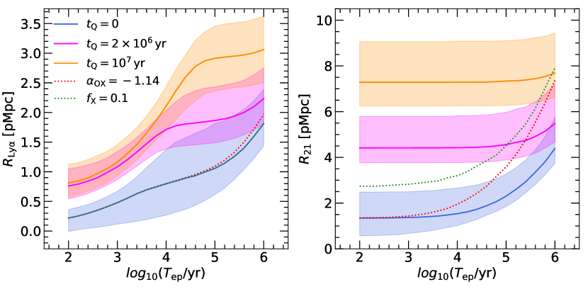
Figure 9: The dependence of $R_{\rm Ly\alpha}$ and $R_{21}$ at $z=7$ on the current episodic lifetime, $T_{\rm ep}$, in a flickering quasar emission model. Results are shown for young quasars in their first bright phase ($t_{\rm Q}=0\rm\,yr$, blue curves), for an intermediate case similar to the lifetime inferred by Morey et al. (2021) ($t_{\rm Q}=10^{6.3}\rm\,yr$, fuchsia curves) and for our fiducial optically/UV bright quasar lifetime ($t_{\rm Q}=10^{7}\rm\,yr$, orange curves). The shading corresponds to the $68$ per cent scatter around the median from 2000 simulated sight lines. Note that while Ly$\alpha$ near-zones can be small ($R_{\rm Ly\alpha}<1\rm\,pMpc$) for all $t_{\rm Q}$ when the quasar has recently entered the bright phase, $R_{21}$ increases monotonically and will be considerably larger than $R_{\rm Ly\alpha}$ for $t_{\rm Q}=10^{7}\rm\,yr$. We also show two additional models in which we boost the X-ray heating in the pre-reionization IGM by setting $f_{\rm X}=0.1$ (dotted green curves) and $\alpha_{\rm OX}=-1.14$ (dotted red curves). Note these curves are almost indistinguishable in the left panel.

We further consider the flickering quasar emission model using the RT-late Sherwood-Relics simulation for $f_{\rm X}=0.01$ and our fiducial SED. In Fig. 9 we show the dependence of the median $R_{\rm Ly\alpha}$ (left panels) and $R_{21}$ (right panels) at $z=7$ on the current episodic lifetime, $T_{\rm ep}$. This is just the duration of the most recent optically/UV bright phase with $M_{1450}=-27$ for a quasar that already has an integrated age $t_{\rm Q}$, with $f_{\rm duty}=0.5$ and $t_{\rm ep}=10^{6}\rm\,yr$. Three different integrated quasar ages are displayed, where $t_{\rm Q}=0\rm\,yr$ (blue curves), $t_{\rm Q}=2\times 10^{6}\rm\,yr$ (fuchsia curves) and $t_{\rm Q}=10^{7}\rm\,yr$ (orange curves), as measured from the start of the most recent optically/UV bright phase (i.e. for $0$, $1$ and $5$ earlier episodic cycles with $t_{\rm ep}=10^{6}\rm\,yr$, respectively). The shaded regions show the 68 per cent scatter around the median.

First, note the $R_{\rm Ly\alpha}$ and $R_{21}$ values for $t_{\rm Q}=0\rm\,yr$ are almost identical to the light bulb model in Fig. 7 (fuchsia curves) for $t_{\rm Q}\leq 10^{6}\rm\,yr$, as should be expected. However, in the case of older quasars with $t_{\rm Q}>t_{\rm ep}$ that have experienced at least one episodic cycle, we find (within the 68 per cent scatter) that $R_{\rm Ly\alpha}\lesssim 2\rm\,pMpc$ for $T_{\rm ep}\sim t_{\rm ion}<10^{4.5}\rm\,yr$, and that $R_{\rm Ly\alpha}$ is insensitive to the integrated quasar age. As already discussed, this is a consequence of the re-equilibriation of the neutral hydrogen behind the quasar H$\,\rm\scriptstyle II$ ionization front during the quasar faint phase. For an episodic lifetime of $t_{\rm ep}=10^{6}\rm\,yr$, we would therefore expect $R_{\rm Ly\alpha,corr}\lesssim 2\rm\,pMpc$ for $\sim 3$ per cent of $z=7$ quasars, even if the integrated quasar age $t_{\rm Q}>t_{\rm ep}$. Similar results have been pointed out elsewhere (e.g. Davies et al., 2020)

On the other hand, as a result of the long cooling timescale for neutral gas ahead of the H$\,\rm\scriptstyle II$ ionization front, $R_{21}$ is $\sim 2$–$5.5$ times larger for $t_{\rm Q}=10^{7}\rm\,yr$ (orange curve) compared to $R_{21}$ for a quasar that has just turned on for the first time (blue curve). Hence, if invoking flickering quasar emission to reconcile the apparent short optically/UV bright lifetimes of quasars at $z\gtrsim 6$ with the build-up of $\sim 10^{9}\rm\,M_{\odot}$ black holes, we expect $R_{21}>R_{\rm Ly\alpha}$. Only for the case of a very young quasar do we find proximate 21-cm absorption with $R_{21}\sim 2\rm\,pMpc$. An important caveat here, however, is the level of X-ray heating in the neutral IGM. The dotted curves show results for $f_{\rm X}=0.1$ or $\alpha_{\rm OX}=-1.14$ for the case of a $t_{\rm Q}=0\rm\,yr$ (i.e. the blue curves for the fiducial model). While $R_{\rm Ly\alpha}$ remains unaffected by X-ray heating, $R_{21}$ increases. Raising the X-ray background efficiency, $f_{\rm X}$, results in a larger initial $R_{21}$, while a harder optical-to-X-ray spectral index, $\alpha_{\rm OX}$, increases $R_{21}$ on timescales $T_{\rm ep}\gtrsim t_{\rm ion}$. Nevertheless, for $t_{\rm Q}\lesssim 10^{4}\rm\,yr$ we still expect $R_{21}\lesssim 3\rm\,pMpc$ if the quasar has not undergone earlier episodic cycles for $M_{\rm AB}=-27$, where the magnitude corrected size scales as $R_{\rm 21,corr}\propto 10^{0.4(27+M_{1450})/3}$ (see Appendix B). Finally, we point out that a null detection of proximate 21-cm absorption with $F_{21}<0.99$ would be indicative of an X-ray background with $f_{\rm X}\gtrsim 1$ at $z=7$ (see fig. 8 in Šoltinský et al., 2021).

In summary, we suggest that a measurement of $R_{21}$ along the line of sight to radio-loud quasars could complement existing constraints on the lifetime of quasars obtained from Ly$\alpha$ transmission. Furthermore, a detection of proximate 21-cm absorption from the diffuse IGM within a few proper Mpc of a bright quasar at $z\simeq 7$ would present yet another challenge for the growth of $\sim 10^{9}\rm\,M_{\odot}$ black holes during the reionization epoch. Our modelling indicates that long range heating by X-ray photons means that for $f_{\rm X}\lesssim 0.1$, $R_{21}\lesssim 2$–$3\rm pMpc$ should only occur for radio-loud quasars that have recently initiated accretion. Larger values of $R_{\rm 21}$ coupled with $R_{\rm Ly\alpha,corr}<2\rm\,pMpc$ would instead hint at black hole growth progressing over timescales much longer than the optically/UV bright lifetimes of $t_{\rm Q}\sim 10^{4}\rm\,yr$ implied by the smallest Ly$\alpha$ near-zone sizes of the quasar population at $z\gtrsim 6$ (Morey et al., 2021).

6 Conclusions

Recent studies have suggested that observed Ly$\alpha$ near-zone sizes at $z\gtrsim 6$ (Fan et al., 2006; Carilli et al., 2010; Willott et al., 2010; Venemans et al., 2015; Reed et al., 2015; Eilers et al., 2017, 2021; Mazzucchelli et al., 2017; Ishimoto et al., 2020) are consistent with an average quasar optically/UV bright lifetime of $t_{\rm Q}\sim 10^{6}\rm\,yr$, with lifetimes as short as $t_{\rm Q}\lesssim 10^{4}$–$10^{5}\rm\,yr$ preferred by the smallest Ly$\alpha$ near-zones at $z\simeq 6$ (Eilers et al., 2017, 2021; Morey et al., 2021). If correct, this presents an apparent challenge for the build-up of $\sim 10^{9}\rm\,M_{\odot}$ supermassive black holes at $z\gtrsim 6$, as the black hole growth e-folding time is at least an order of magnitude larger than $t_{\rm Q}$ if assuming Eddington limited accretion. These very young quasars would need to have grown from very massive seeds through radiatively inefficient, super Eddington accretion (Madau et al., 2014; Davies et al., 2019). Note, however, that because the number of black holes implied by the detected optically/UV bright quasars scales inversely with the optically/UV bright lifetime (e.g. Haehnelt et al., 1998), this would also push the quasars into rather low mass haloes. Alternatively, the quasars could be much older and have only recently entered an optically/UV bright phase. This is possible if most quasars at $z\gtrsim 6$ grow primarily in an optical/UV obscured phase (Hopkins et al., 2005; Ricci et al., 2017), or variable accretion causes them to "flicker” between optically/UV bright and faint states on episodic timescales $t_{\rm ep}\sim 10^{5}$–$10^{6}\rm\,yr$ (Schawinski et al., 2015; Shen, 2021). Distinguishing between these possibilities with Ly$\alpha$ near-zones is difficult, however, due to the relatively short equilibriation timescale, $t_{\rm eq}\sim 10^{5}\rm\,yr$, for the residual neutral hydrogen surrounding the quasar (Davies et al., 2020).

In this work, we have therefore used the Sherwood-Relics simulations of inhomogeneous reionization (Puchwein et al., 2022), coupled with line of sight radiative transfer calculations, to model the Ly$\alpha$ and 21-cm absorption in close proximity to $z\gtrsim 6$ quasars. The empirically calibrated reionization histories available in the Sherwood-Relics simulation suite and the flexibility of our line of sight radiative transfer algorithm allows us to explore a large parameter space, including variations in the IGM neutral fraction, the X-ray background intensity, and the quasar age and spectral shape. We suggest that the observation of proximate 21-cm absorption in the spectra of radio-loud quasars at $z\gtrsim 6$ (with e.g. SKA1-low or SKA2) could provide a route for probing the lifetimes of $z\gtrsim 6$ quasars that is complementary to Ly$\alpha$ near-zones and proposed analyses of quasar H$\,\rm\scriptstyle II$ regions using 21-cm tomography (e.g. Wyithe & Loeb, 2004b; Kohler et al., 2005; Rhook & Haehnelt, 2006; Geil & Wyithe, 2008; Majumdar et al., 2012; Datta et al., 2012; Kakiichi et al., 2017; Ma et al., 2020; Davies et al., 2021). Our main conclusions are as follows:

• If allowing for a distribution of optically/UV bright lifetimes with a median of $t_{\rm Q}\simeq 10^{6}\rm\,yr$ (Morey et al., 2021), the luminosity corrected sizes of Ly$\alpha$ near-zones, $R_{\rm Ly\alpha,corr}$, are reasonably well reproduced within the Sherwood-Relics simulations for a model with late reionization ending at $z=5.3$. Slightly larger average lifetimes may be allowable within late reionization models (e.g. Satyavolu et al., 2022), although in the models presented here the effect is modest and differences are within the 68 per cent scatter around the predicted median $R_{\rm Ly\alpha}$ (compare e.g. RT-late and RT-mid in Fig. 5). We also confirm that the smallest Ly$\alpha$ near-zones at $z\simeq 6$, with quasar luminosity corrected sizes of $R_{\rm Ly\alpha,corr}\lesssim 2\rm\,pMpc$, are consistent with optically/UV bright quasar lifetimes of $t_{\rm Q}\lesssim 10^{4}$–$10^{5}\rm\,yr$ in late reionization models (Eilers et al., 2017, 2021).
  

• We define the “21-cm near-zone” size, $R_{21}$, as the distance from a (radio-loud) quasar where the normalised 21-cm forest spectrum first drops below the threshold $F_{\rm 21,th}=0.99$ (i.e $\tau_{21}\gtrsim 10^{-2}$), after smoothing the radio spectrum with a $5\rm\,kHz$ boxcar filter. Detecting a strong proximate 21-cm absorber with $\tau_{21}\geq 10^{-2}$ requires a minimum source flux density of 17.2 mJy (5.9 mJy) for a 1000 (100) hour integration with SKA1-low (SKA2), assuming a signal-to-noise ratio of $\rm S/N=5$ and bandwidth of $5\rm\,kHz$. For comparison, the recently discovered radio-loud quasar PSO J172+18 has a $3\sigma$ upper limit on the flux density at $147.5\rm\,MHz$ of $S_{147.5\rm\,MHz}<8.5\rm\,mJy$ (Bañados et al., 2021), and the blazar PSO J0309+27 at $z=6.1$ has $S_{147\rm\,MHz}=64.2\pm 6.2\rm\,mJy$ (Belladitta et al., 2020). Proximate 21-cm absorption around these or similar radio-loud sources should therefore be within reach of the SKA.
  

• We show that for modest pre-heating of the IGM by the X-ray background, such that the IGM spin temperature $T_{\rm S}\lesssim 10^{2}\rm\,K$, strong proximate 21-cm absorption from the diffuse IGM should be present in the spectra of radio-loud quasars (see also Šoltinský et al., 2021). We demonstrate that $R_{21}$ will depend on the quasar optical-to-X-ray spectral index, $\alpha_{\rm OX}$, and the integrated quasar lifetime, $t_{\rm Q}$. In contrast, the Ly$\alpha$ near-zone size remains insensitive to the level of X-ray heating in the IGM. For very young quasars, $R_{21}$ should trace the extent of the pre-existing H$\,\rm\scriptstyle II$ regions created by galaxies clustered around the quasar host halo.
  

• Unlike the Ly$\alpha$ near-zone size – which can vary over the equilibriation timescale, $t_{\rm eq}\sim 10^{5}\rm\,yr$, for neutral hydrogen in a highly ionized IGM (e.g. Davies et al., 2020) – $R_{21}$ is sensitive to the integrated lifetime of the quasar and will increase monotonically with quasar age. This is because the 21-cm optical depth is inversely proportional to the spin temperature of neutral hydrogen, $\tau_{21}\propto T_{\rm S}^{-1}$, and the neutral hydrogen will cool adiabatically on a timescale $t_{\rm H}/2$, where $t_{\rm H}\gg t_{\rm Q}$ is the Hubble time. A combination of $R_{21}$ and $R_{\rm Ly\alpha}$ may therefore help sharpen constraints on quasar lifetimes if the uncertain heating by X-rays from the quasar and X-ray background can be marginalised over.
  

• For quasars that exhibit unusually small luminosity corrected Ly$\alpha$ near-zone sizes (where evidence for a Ly$\alpha$ damping wing from a large neutral column in the IGM may also be limited), proximate 21-cm absorption could help distinguish between very young quasars with $t_{\rm Q}<10^{4}$–$10^{5}\rm\,yr$, or older quasars that have experienced episodic accretion. We find that proximate 21-cm absorption from the diffuse IGM is only expected within a few proper Mpc of the quasar systemic redshift for very young objects. Such short lifetimes may point toward massive black hole seeds (e.g. Loeb & Rasio, 1994; Dijkstra et al., 2008; Regan et al., 2017) and radiatively inefficient, mildly super-Eddington accretion (Madau et al., 2014; Davies et al., 2019). Larger values of $R_{21}$ coupled with small Ly$\alpha$ near-zones with $R_{\rm Ly\alpha,corr}\lesssim 2\rm\,pMpc$ would instead be consistent with time-variable black hole growth occurring over longer periods.

Our results provide further impetus for searching for 21-cm absorption from the diffuse IGM at high redshift. However, the caveats discussed by our earlier work focusing on 21-cm absorption from the general IGM (Šoltinský et al., 2021) also apply here. We have not considered any of the practical issues regarding the recovery of 21-cm absorption features from noisy data. The role of 21-cm absorption from any minihaloes that are unresolved in our simulations (i.e. minihaloes with masses $<2.5\times 10^{7}\rm\,M_{\odot}$) also remains uncertain (Meiksin, 2011; Park et al., 2016; Nakatani et al., 2020). Soft X-ray heating of the IGM by the transverse quasar proximity effect may also be an important uncertainty, particularly for the large population of faint or obscured quasars that would be implied by short optically/UV bright quasar lifetimes and/or duty cycles. Finally, note that if the neutral IGM is already pre-heated to temperatures $T\gg 10^{2}\rm\,K$ at $z\gtrsim 6$, there will be very little or no detectable 21-cm absorption from the diffuse IGM at all. Although constraints on the X-ray background and spin temperature in the IGM are still weak (Greig et al., 2021; The HERA Collaboration, 2022), further progress toward placing limits and/or detecting the 21-cm power spectrum should help narrow parameter space over the next decade.

Data Availability

All data and analysis code used in this work are available from the first author on request.

Appendix A The dependence of $R_{21}$ on transmission threshold

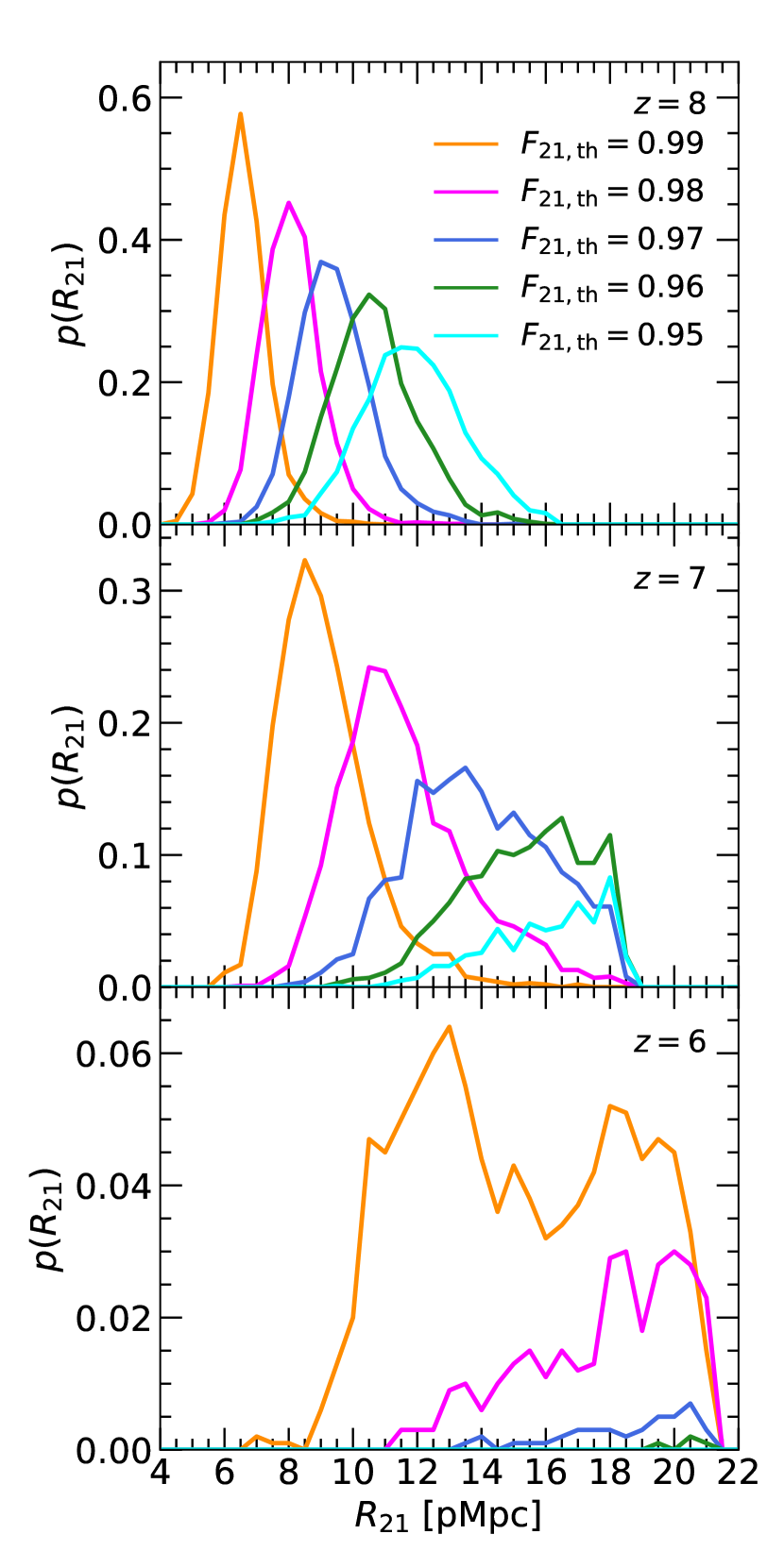
Figure 10: The probability distribution of $R_{21}$ assuming different values for distance from the quasar at which the 21-cm transmission first drops below $F_{\rm 21,th}$, after smoothing the 21-cm spectrum with a boxcar filter of width $5\rm\,kHz$. The results are shown for our fiducial model for 2000 sight lines at $z=8$, 7 and 6. The orange curves for $F_{\rm 21,th}=0.99$ are the same as the solid curves shown in the lower left panel of Fig. 6. Note the different scale on the vertical axes of each panel; many sight lines at $z=6$ show no 21-cm absorption with $F<F_{\rm 21,th}$. Additionally, the length of the simulated sight-lines is $100h^{-1}\rm\,cMpc$, so there is an artificial cut-off in the distributions at $R_{21}=[16.4,\,18.4,\,21.1]\rm\,pMpc$ at $z=[8,\,7,\,6]$.

Table 2: The minimum flux density required to detect a 21-cm forest absorption feature with $F_{\rm 21,th}$ with $\rm S/N=5$ using SKA1-low (middle column) or SKA2 (right column). This has been calculated from Eq. (3.2) assuming a bandwidth of $\Delta\nu=5\rm\,kHz$, sensitivity $A_{\rm eff}/T_{\rm sys}=600\rm\,m^{2}\,K^{-1}$ $\left(5500\rm\,m^{2}\,K^{-1}\right)$ (Braun et al., 2019) and an integration time of $t_{\rm int}=1000\rm\,hr$ $\left(100\rm\,hr\right)$ for SKA1-low (SKA2).

$F_{\rm 21,th}$	$S_{\rm min}/\rm\,mJy,\,SKA1-low$	$S_{\rm min}/\rm\,mJy,\,SKA2$
0.99	17.2	5.9
0.98	8.6	3.0
0.97	5.7	2.0
0.96	4.3	1.5
0.95	3.4	1.2

In analogy to the widely used definition for $R_{\rm Ly\alpha}$ (e.g. Fan et al., 2006), our definition of $R_{21}$ is practical rather than physically motivated. The choice of $F_{\rm 21,th}=0.99$ as the transmission threshold where we define $R_{21}$ is somewhat arbitrary. Here we show how a different choice of $F_{\rm 21,th}$ affects our results. Fig. 10 shows the distribution of $R_{21}$ in our fiducial RT-late reionization model at redshift $z=8$, 7 and 6, assuming a range of $F_{\rm 21,th}$ values. We have assumed $M_{1450}=-27$, $f_{\rm X}=0.01$, $t_{\rm Q}=10^{7}\rm\,yr$ and our fiducial quasar SED in the models. Decreasing $F_{\rm 21,th}$ shifts the $R_{21}$ distribution to larger values, consistent with the expectation that stronger 21-cm absorption features should appear further from the quasar due to the lower spin temperatures (see e.g. Fig. 2).

In addition, note that while we find absorption features with $F_{\rm 21,th}\geq 0.98$ in almost all sight lines at $z=7$, only $62$ per cent contain features with $F_{\rm 21,th}=0.96$, and this further decreases to $26$ per cent for $F_{\rm 21,th}=0.95$. In Table 2, we list the minimum intrinsic flux density that a radio source must have for SKA1-low or SKA2 to detect a 21-cm forest absorber with $F_{\rm 21,th}$ at a signal-to-noise ratio of $\rm S/N=5$. Here we use Eq. (3.2), and assume $A_{\rm eff}/T_{\rm sys}=600\rm\,m^{2}\,K^{-1}$ and $t_{\rm int}=1000\rm\,hr$ for SKA1-low and $A_{\rm eff}/T_{\rm sys}=5500\rm\,m^{2}\,K^{-1}$ and $t_{\rm int}=100\rm\,hr$ for SKA2, and a bandwidth of $\Delta\nu=5\rm\,kHz$.

Appendix B The dependence of $R_{21}$ on quasar magnitude

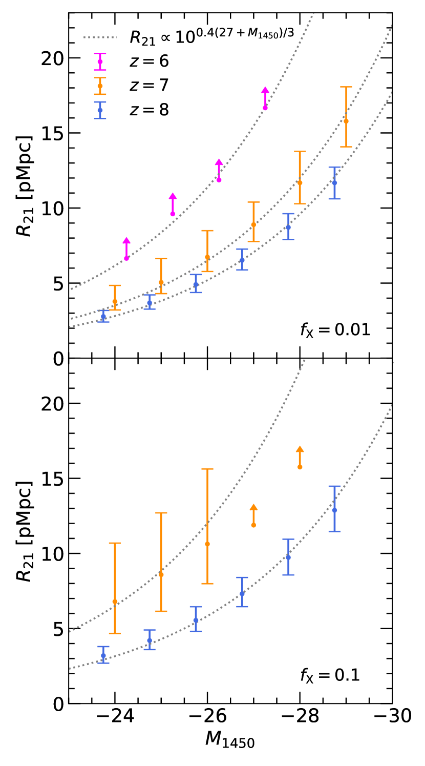
Figure 11: The 21-cm near-zone size, $R_{21}$, as a function of the quasar magnitude, $M_{1450}$, at $\rm z=6$ (fuchsia points), $z=7$ (orange points) and $z=8$ (blue points) in the RT-late model. The fiducial SED and optically/UV bright lifetime of $t_{\rm Q}=10^{7}\rm\,yr$ are assumed, for an X-ray background efficiency $f_{\rm X}=0.01$ (upper panel) and $f_{\rm X}=0.1$ (lower panel). The data points correspond to the median and $68$ per cent range for $2000$ simulated quasar sight-lines. Arrows indicate the $68$ per cent lower limit for $\rm R_{21}$ when multiple sight-lines have no pixels with $F_{\rm 21,th}<0.99$. The points are slightly offset on the horizontal axes for presentation purposes. The grey dotted curves show $R_{21}\propto 10^{0.4(27+M_{1450})/3}$, which is the expected scaling for an H$\,\rm\scriptstyle II$ region (i.e. $R_{21}\propto\dot{N}^{1/3}$). Note also there are no sight-lines with $F_{\rm 21,th}<0.99$ for $f_{\rm X}=0.1$ at $z=6$.

The dependence of $R_{\rm Ly\alpha}$ on the quasar magnitude, $M_{1450}$ (or equivalently the ionizing photon emission rate, $\dot{N}$) has been discussed extensively elsewhere (e.g. Bolton & Haehnelt, 2007; Davies et al., 2020; Ishimoto et al., 2020; Satyavolu et al., 2022). In particular, Eilers et al. (2017) derived the scaling relation in Eq. (7) using their radiative transfer simulations. Analogously, we present the dependence of $R_{21}$ on $M_{1450}$ in Fig. 11 for $f_{\rm X}=0.01$ (top panel) and $f_{\rm X}=0.1$ (bottom panel) at $z=6$ (fuchsia points), $z=7$ (orange points) and $z=8$ (blue points) for a quasar with an optically/UV bright lifetime of $t_{\rm Q}=10^{7}\rm\,yr$. The error bars show the 68 per cent scatter around the median obtained from $2000$ simulated sight lines, and the arrows show $68$ per cent lower limits.

We find $R_{21}\propto 10^{0.4(27+M_{1450})/3}\propto\dot{N}^{1/3}$ (dashed grey curves) is consistent with the simulations, in agreement with the expected scaling for the expansion of a quasar H$\,\rm\scriptstyle II$ region given by Eq. (12) (although note, as discussed earlier, $R_{21}$ does not necessarily correspond to $R_{\rm HII}$ – it instead roughly corresponds to the size of the region heated to $T_{\rm S}\gtrsim 100\rm\,K$ by the quasar). The only exception is for $f_{\rm X}=0.1$ at $z=6$, where proximate 21-cm absorption is very rare due to the heating of the remaining neutral gas in the IGM to spin temperatures $T_{\rm S}\gtrsim 10^{2}\rm\,K$. In this case only $\sim 0.2$ per cent of our $2000$ synthetic spectra have $R_{21}<21\rm\,pMpc$ for $M_{1450}>-27$, and even fewer for more luminous quasars. For comparison, Šoltinský et al. (2021) infer a lower limit of $f_{\rm X}>0.109$ assuming a null detection of 21-cm absorption with $F_{21}\leq 0.99$ over a path length of $5.8h^{-1}\rm\,cGpc$ ($\Delta z=20$) at $z=6$ (see their table 2). However, these numbers are for the general IGM, and exclude the effect of localised ionization and heating in close proximity to bright sources. Here, over our simulated path length of $200h^{-1}\rm\,cGpc$ ($\Delta z=687.9$) at $z=6$, from Šoltinský et al. (2021) we would naively expect $\sim 34$ 21-cm absorbers with $F_{\rm 21}<0.99$. Instead, we find only 3 absorbers. This difference is largely due to the soft X-ray heating by the quasars reducing the incidence of the proximate 21-cm absorbers, and the rapid redshift evolution of the average IGM neutral fraction along our $100h^{-1}\rm\,cMpc$ sight lines.

Appendix C The quasar lifetime distribution obtained from Ly$\alpha$ near-zone sizes

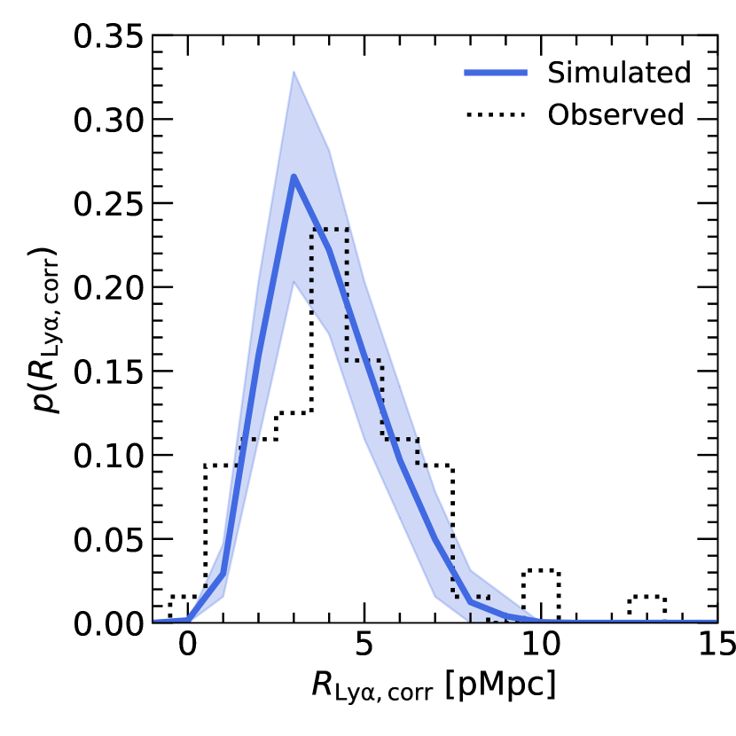
Figure 12: The probability distribution for (luminosity corrected) Ly$\alpha$ near-zone sizes (blue solid curve) at $z=6$ from radiative transfer simulations using our fiducial model the quasar lifetime distribution from Morey et al. (2021). The shaded region shows the $1\sigma$ uncertainty obtained by bootstrapping. For comparison, the $R_{\rm Ly\alpha,corr}$ distribution from observed quasars in the redshift range $5.8\leq z\leq 6.6$ is shown by the dotted histogram.

Morey et al. (2021) have recently demonstrated that the majority of $R_{\rm Ly\alpha,\rm corr}$ measurements at $z\simeq 6$ are reproduced assuming a median optically/UV bright lifetime of $t_{\rm Q}=10^{5.7}\rm\,yr$ with a $95$ per cent confidence interval $t_{\rm Q}=10^{5.3}$–$10^{6.5}\rm\,yr$ (see their fig. 6). We test this in Fig. 12, where instead of using a single value for $t_{\rm Q}$ in our simulations, we adopt values using the posterior probability distribution for the quasar lifetimes inferred by Morey et al. (2021). We select 2000 quasar lifetime values from their distribution using a Monte Carlo rejection method. Each simulated sight line was then randomly assigned a different $t_{\rm Q}$ from this sample. We then performed 2000 radiative transfer simulations of our fiducial model at $z=6$, and bootstrapped $10^{4}$ sets of sight lines from these simulations to obtain a $1\sigma$ uncertainty. Each bootstrapped set contains 64 synthetic sight lines, corresponding to the number of quasars in the compiled observational sample we use for quasars at $5.8\leq z\leq 6.6$.

The dotted black curve in Fig. 12 shows the observed distribution of luminosity corrected Ly$\alpha$ near-zone sizes at $5.8\leq z\leq 6.6$. The solid blue curve corresponds to the median and $1\sigma$ uncertainty obtained by bootstrapping our simulations. A two-sided Kolmogorov-Smirnov test yields a p-value of $0.055$, which remains consistent ($p>0.05$) with the null-hypothesis that the samples are drawn from the same distribution. There is a hint that the simulated near-zone sizes are slightly smaller than the observational data, which may be a result of applying the Morey et al. (2021) $t_{\rm Q}$ distribution to our late reionization model (see also Satyavolu et al., 2022). Our RT-late simulation has a larger average IGM neutral fraction at $z=6$ compared to the models used by Morey et al. (2021), which assumes a fully ionized IGM. However, this difference is not highly significant.

References

- Anglés-Alcázar et al. (2017) Anglés-Alcázar D., Faucher-Giguère C.-A., Quataert E., Hopkins P. F., Feldmann R., Torrey P., Wetzel A., Kereš D., 2017, MNRAS, 472, L109
- Astropy Collaboration et al. (2013) Astropy Collaboration et al., 2013, A&A, 558, A33
- Aubert & Teyssier (2008) Aubert D., Teyssier R., 2008, MNRAS, 387, 295
- Bañados et al. (2018) Bañados E., et al., 2018, Nature, 553, 473
- Bañados et al. (2021) Bañados E., et al., 2021, ApJ, 909, 80
- Bajtlik et al. (1988) Bajtlik S., Duncan R. C., Ostriker J. P., 1988, ApJ, 327, 570
- Becker et al. (2015a) Becker G. D., Bolton J. S., Lidz A., 2015a, Publ. Astron. Soc. Australia, 32, e045
- Becker et al. (2015b) Becker G. D., Bolton J. S., Madau P., Pettini M., Ryan-Weber E. V., Venemans B. P., 2015b, MNRAS, 447, 3402
- Belladitta et al. (2020) Belladitta S., et al., 2020, A&A, 635, L7
- Bolton & Haehnelt (2007) Bolton J. S., Haehnelt M. G., 2007, MNRAS, 374, 493
- Bolton et al. (2011) Bolton J. S., Haehnelt M. G., Warren S. J., Hewett P. C., Mortlock D. J., Venemans B. P., McMahon R. G., Simpson C., 2011, MNRAS, 416, L70
- Bolton et al. (2012) Bolton J. S., Becker G. D., Raskutti S., Wyithe J. S. B., Haehnelt M. G., Sargent W. L. W., 2012, MNRAS, 419, 2880
- Bosman (2022) Bosman S. E. I., 2022, All z>5.7 quasars currently known, doi:10.5281/zenodo.6039724
- Bosman & Becker (2015) Bosman S. E. I., Becker G. D., 2015, MNRAS, 452, 1105
- Bosman et al. (2018) Bosman S. E. I., Fan X., Jiang L., Reed S., Matsuoka Y., Becker G., Haehnelt M., 2018, MNRAS, 479, 1055
- Bosman et al. (2022) Bosman S. E. I., et al., 2022, MNRAS, 514, 55
- Braun et al. (2019) Braun R., Bonaldi A., Bourke T., Keane E., Wagg J., 2019, arXiv e-prints, p. arXiv:1912.12699
- Calverley et al. (2011) Calverley A. P., Becker G. D., Haehnelt M. G., Bolton J. S., 2011, MNRAS, 412, 2543–2562
- Carilli et al. (2002) Carilli C. L., Gnedin N. Y., Owen F., 2002, ApJ, 577, 22
- Carilli et al. (2010) Carilli C. L., et al., 2010, ApJ, 714, 834
- Cen & Haiman (2000) Cen R., Haiman Z., 2000, ApJ, 542, L75
- Chen & Gnedin (2021) Chen H., Gnedin N. Y., 2021, ApJ, 911, 60
- Chen et al. (2022) Chen H., et al., 2022, ApJ, 931, 29
- Choudhury et al. (2021) Choudhury T. R., Paranjape A., Bosman S. E. I., 2021, MNRAS, 501, 5782
- Ciardi et al. (2013) Ciardi B., et al., 2013, MNRAS, 428, 1755
- Connor et al. (2021) Connor T., et al., 2021, ApJ, 911, 120
- Datta et al. (2012) Datta K. K., Friedrich M. M., Mellema G., Iliev I. T., Shapiro P. R., 2012, MNRAS, 424, 762
- Davies et al. (2018) Davies F. B., et al., 2018, ApJ, 864, 142
- Davies et al. (2019) Davies F. B., Hennawi J. F., Eilers A.-C., 2019, ApJ, 884, L19
- Davies et al. (2020) Davies F. B., Hennawi J. F., Eilers A.-C., 2020, MNRAS, 493, 1330
- Davies et al. (2021) Davies J. E., Croft R. A. C., Di-Matteo T., Greig B., Feng Y., Wyithe J. S. B., 2021, MNRAS, 501, 146
- Dijkstra et al. (2008) Dijkstra M., Haiman Z., Mesinger A., Wyithe J. S. B., 2008, MNRAS, 391, 1961
- D’Aloisio et al. (2019) D’Aloisio A., McQuinn M., Maupin O., Davies F. B., Trac H., Fuller S., Upton Sanderbeck P. R., 2019, ApJ, 874, 154
- Eilers et al. (2017) Eilers A.-C., Davies F. B., Hennawi J. F., Prochaska J. X., Lukić Z., Mazzucchelli C., 2017, ApJ, 840, 24
- Eilers et al. (2018) Eilers A.-C., Davies F. B., Hennawi J. F., 2018, ApJ, 864, 53
- Eilers et al. (2020) Eilers A.-C., et al., 2020, ApJ, 900, 37
- Eilers et al. (2021) Eilers A.-C., Hennawi J. F., Davies F. B., Simcoe R. A., 2021, ApJ, 917, 38
- Fan et al. (2006) Fan X., et al., 2006, AJ, 132, 117
- Farina et al. (2022) Farina E. P., et al., 2022, arXiv e-prints, p. arXiv:2207.05113
- Finlator et al. (2018) Finlator K., Keating L., Oppenheimer B. D., Davé R., Zackrisson E., 2018, MNRAS, 480, 2628
- Furlanetto (2006a) Furlanetto S. R., 2006a, MNRAS, 370, 1867
- Furlanetto (2006b) Furlanetto S. R., 2006b, MNRAS, 371, 867
- Furlanetto & Loeb (2002) Furlanetto S. R., Loeb A., 2002, ApJ, 579, 1
- Furlanetto & Stoever (2010) Furlanetto S. R., Stoever S. J., 2010, MNRAS, 404, 1869
- Furlanetto et al. (2004) Furlanetto S. R., Zaldarriaga M., Hernquist L., 2004, ApJ, 613, 16
- Gaikwad et al. (2020) Gaikwad P., et al., 2020, MNRAS, 494, 5091
- Garaldi et al. (2022) Garaldi E., Kannan R., Smith A., Springel V., Pakmor R., Vogelsberger M., Hernquist L., 2022, MNRAS, 512, 4909
- Geil & Wyithe (2008) Geil P. M., Wyithe J. S. B., 2008, MNRAS, 386, 1683
- Gloudemans et al. (2022) Gloudemans A. J., et al., 2022, A&A, 668, A27
- Gnedin (2014) Gnedin N. Y., 2014, ApJ, 793, 29
- Greig et al. (2017) Greig B., Mesinger A., Haiman Z., Simcoe R. A., 2017, MNRAS, 466, 4239
- Greig et al. (2021) Greig B., Trott C. M., Barry N., Mutch S. J., Pindor B., Webster R. L., Wyithe J. S. B., 2021, MNRAS, 500, 5322
- Greig et al. (2022) Greig B., Mesinger A., Davies F. B., Wang F., Yang J., Hennawi J. F., 2022, MNRAS, 512, 5390
- Haehnelt et al. (1998) Haehnelt M. G., Natarajan P., Rees M. J., 1998, MNRAS, 300, 817
- Harris et al. (2020) Harris C. R., et al., 2020, Nature, 585, 357
- Hopkins et al. (2005) Hopkins P. F., Hernquist L., Martini P., Cox T. J., Robertson B., Di Matteo T., Springel V., 2005, ApJ, 625, L71
- Hsyu et al. (2020) Hsyu T., Cooke R. J., Prochaska J. X., Bolte M., 2020, ApJ, 896, 77
- Hunter (2007) Hunter J. D., 2007, Computing in Science and Engineering, 9, 90
- Ighina et al. (2021) Ighina L., Belladitta S., Caccianiga A., Broderick J. W., Drouart G., Moretti A., Seymour N., 2021, A&A, 647, L11
- Iliev et al. (2014) Iliev I. T., Mellema G., Ahn K., Shapiro P. R., Mao Y., Pen U.-L., 2014, MNRAS, 439, 725
- Inayoshi et al. (2020) Inayoshi K., Visbal E., Haiman Z., 2020, ARA&A, 58, 27
- Ishimoto et al. (2020) Ishimoto R., et al., 2020, ApJ, 903, 60
- Kakiichi et al. (2017) Kakiichi K., et al., 2017, MNRAS, 471, 1936
- Kaur et al. (2020) Kaur H. D., Gillet N., Mesinger A., 2020, MNRAS, 495, 2354
- Keating et al. (2015) Keating L. C., Haehnelt M. G., Cantalupo S., Puchwein E., 2015, MNRAS, 454, 681
- Keating et al. (2020) Keating L. C., Weinberger L. H., Kulkarni G., Haehnelt M. G., Chardin J., Aubert D., 2020, MNRAS, 491, 1736
- Khrykin et al. (2019) Khrykin I. S., Hennawi J. F., Worseck G., 2019, MNRAS, 484, 3897
- Khrykin et al. (2021) Khrykin I. S., Hennawi J. F., Worseck G., Davies F. B., 2021, MNRAS, 505, 649
- King & Nixon (2015) King A., Nixon C., 2015, MNRAS, 453, L46
- Knevitt et al. (2014) Knevitt G., Wynn G. A., Power C., Bolton J. S., 2014, MNRAS, 445, 2034
- Kohler et al. (2005) Kohler K., Gnedin N. Y., Miralda-Escudé J., Shaver P. A., 2005, ApJ, 633, 552
- Kroupa et al. (2020) Kroupa P., Subr L., Jerabkova T., Wang L., 2020, MNRAS, 498, 5652
- Kulkarni et al. (2019) Kulkarni G., Keating L. C., Haehnelt M. G., Bosman S. E. I., Puchwein E., Chardin J., Aubert D., 2019, MNRAS, 485, L24
- Lewis et al. (2022) Lewis J. S. W., et al., 2022, MNRAS, 516, 3389
- Lidz et al. (2007) Lidz A., McQuinn M., Zaldarriaga M., Hernquist L., Dutta S., 2007, ApJ, 670, 39
- Liu et al. (2021) Liu Y., et al., 2021, ApJ, 908, 124
- Loeb & Rasio (1994) Loeb A., Rasio F. A., 1994, ApJ, 432, 52
- Lusso et al. (2010) Lusso E., et al., 2010, A&A, 512, A34
- Lusso et al. (2015) Lusso E., Worseck G., Hennawi J. F., Prochaska J. X., Vignali C., Stern J., O’Meara J. M., 2015, MNRAS, 449, 4204
- Ma et al. (2020) Ma Q.-B., Ciardi B., Kakiichi K., Zaroubi S., Zhi Q.-J., Busch P., 2020, ApJ, 888, 112
- Mack & Wyithe (2012) Mack K. J., Wyithe J. S. B., 2012, MNRAS, 425, 2988
- Madau & Rees (2000) Madau P., Rees M. J., 2000, ApJ, 542, L69
- Madau et al. (1997) Madau P., Meiksin A., Rees M. J., 1997, ApJ, 475, 429
- Madau et al. (2014) Madau P., Haardt F., Dotti M., 2014, ApJ, 784, L38
- Majumdar et al. (2012) Majumdar S., Bharadwaj S., Choudhury T. R., 2012, MNRAS, 426, 3178
- Martini (2004) Martini P., 2004, in Ho L. C., ed., Coevolution of Black Holes and Galaxies. p. 169 (arXiv:astro-ph/0304009)
- Maselli et al. (2007) Maselli A., Gallerani S., Ferrara A., Choudhury T. R., 2007, MNRAS, 376, L34
- Mazzucchelli et al. (2017) Mazzucchelli C., et al., 2017, ApJ, 849, 91
- Meiksin (2011) Meiksin A., 2011, MNRAS, 417, 1480
- Mesinger & Furlanetto (2008) Mesinger A., Furlanetto S. R., 2008, MNRAS, 385, 1348
- Miralda-Escudé & Rees (1998) Miralda-Escudé J., Rees M. J., 1998, ApJ, 497, 21
- Molaro et al. (2022) Molaro M., et al., 2022, MNRAS, 509, 6119
- Morey et al. (2021) Morey K. A., Eilers A.-C., Davies F. B., Hennawi J. F., Simcoe R. A., 2021, ApJ, 921, 88
- Mortlock et al. (2011) Mortlock D. J., et al., 2011, Nature, 474, 616
- Murdoch et al. (1986) Murdoch H. S., Hunstead R. W., Pettini M., Blades J. C., 1986, ApJ, 309, 19
- Nakatani et al. (2020) Nakatani R., Fialkov A., Yoshida N., 2020, ApJ, 905, 151
- Nasir & D’Aloisio (2020) Nasir F., D’Aloisio A., 2020, MNRAS, 494, 3080
- Oñorbe et al. (2019) Oñorbe J., Davies F. B., Lukić Z., Hennawi J. F., Sorini D., 2019, MNRAS, 486, 4075
- Ocvirk et al. (2021) Ocvirk P., Lewis J. S. W., Gillet N., Chardin J., Aubert D., Deparis N., Thélie É., 2021, MNRAS, 507, 6108
- Park et al. (2016) Park H., Shapiro P. R., Choi J.-h., Yoshida N., Hirano S., Ahn K., 2016, ApJ, 831, 86
- Planck Collaboration (2014) Planck Collaboration 2014, A&A, 571, A16
- Puchwein et al. (2019) Puchwein E., Haardt F., Haehnelt M. G., Madau P., 2019, MNRAS, 485, 47
- Puchwein et al. (2022) Puchwein E., et al., 2022, arXiv e-prints, p. arXiv:2207.13098
- Qin et al. (2021) Qin Y., Mesinger A., Bosman S. E. I., Viel M., 2021, MNRAS, 506, 2390
- Reed et al. (2015) Reed S. L., et al., 2015, MNRAS, 454, 3952
- Regan et al. (2017) Regan J. A., Visbal E., Wise J. H., Haiman Z., Johansson P. H., Bryan G. L., 2017, Nature Astronomy, 1, 0075
- Rhook & Haehnelt (2006) Rhook K. J., Haehnelt M. G., 2006, MNRAS, 373, 623
- Ricci et al. (2017) Ricci C., et al., 2017, MNRAS, 468, 1273
- Salpeter (1964) Salpeter E. E., 1964, ApJ, 140, 796
- Satyavolu et al. (2022) Satyavolu S., Kulkarni G., Keating L. C., Haehnelt M. G., 2022, arXiv e-prints, p. arXiv:2209.08103
- Schawinski et al. (2015) Schawinski K., Koss M., Berney S., Sartori L. F., 2015, MNRAS, 451, 2517
- Semelin (2016) Semelin B., 2016, MNRAS, 455, 962
- Shakura & Sunyaev (1973) Shakura N. I., Sunyaev R. A., 1973, A&A, 24, 337
- Shapiro & Giroux (1987) Shapiro P. R., Giroux M. L., 1987, ApJ, 321, L107
- Shen (2021) Shen Y., 2021, ApJ, 921, 70
- Shen et al. (2007) Shen Y., et al., 2007, AJ, 133, 2222
- Shen et al. (2020) Shen X., Hopkins P. F., Faucher-Giguère C.-A., Alexander D. M., Richards G. T., Ross N. P., Hickox R. C., 2020, MNRAS, 495, 3252
- Springel (2005) Springel V., 2005, MNRAS, 364, 1105
- Steffen et al. (2006) Steffen A. T., Strateva I., Brandt W. N., Alexander D. M., Koekemoer A. M., Lehmer B. D., Schneider D. P., Vignali C., 2006, AJ, 131, 2826
- Šoltinský et al. (2021) Šoltinský T., et al., 2021, MNRAS, 506, 5818
- Tepper-García (2006) Tepper-García T., 2006, MNRAS, 369, 2025
- The HERA Collaboration (2022) The HERA Collaboration 2022, arXiv e-prints, p. arXiv:2210.04912
- Venemans et al. (2015) Venemans B. P., et al., 2015, ApJ, 801, L11
- Viel et al. (2004) Viel M., Haehnelt M. G., Springel V., 2004, MNRAS, 354, 684
- Villanueva-Domingo & Ichiki (2022) Villanueva-Domingo P., Ichiki K., 2022, PASJ
- Virtanen et al. (2020) Virtanen P., et al., 2020, Nature Methods, 17, 261
- Vito et al. (2019) Vito F., et al., 2019, A&A, 630, A118
- Volonteri et al. (2015) Volonteri M., Silk J., Dubus G., 2015, ApJ, 804, 148
- Wang et al. (2020) Wang F., et al., 2020, ApJ, 896, 23
- Wang et al. (2021) Wang F., et al., 2021, ApJ, 908, 53
- Willott et al. (2010) Willott C. J., et al., 2010, AJ, 140, 546
- Worseck et al. (2021) Worseck G., Khrykin I. S., Hennawi J. F., Prochaska J. X., Farina E. P., 2021, MNRAS, 505, 5084
- Wyithe (2008) Wyithe J. S. B., 2008, MNRAS, 387, 469
- Wyithe & Loeb (2004a) Wyithe J. S. B., Loeb A., 2004a, Nature, 427, 815
- Wyithe & Loeb (2004b) Wyithe J. S. B., Loeb A., 2004b, Nature, 432, 194
- Wyithe et al. (2008) Wyithe J. S. B., Bolton J. S., Haehnelt M. G., 2008, MNRAS, 383, 691
- Xu et al. (2011) Xu Y., Ferrara A., Chen X., 2011, MNRAS, 410, 2025
- Yang et al. (2020a) Yang J., et al., 2020a, ApJ, 897, L14
- Yang et al. (2020b) Yang J., et al., 2020b, ApJ, 904, 26
- Yu & Tremaine (2002) Yu Q., Tremaine S., 2002, MNRAS, 335, 965
- Zhu et al. (2022) Zhu Y., et al., 2022, ApJ, 932, 76