Maximal Entangling Rates from Holography

Abstract

We prove novel speed limits on the growth of entanglement, equal-time correlators, and spacelike Wilson loops in spatially uniform time-evolving states in strongly coupled CFTs with holographic duals. These bounds can also be viewed as quantum weak energy conditions. Several of the speed limits are valid for regions of arbitrary size and with multiple connected components, and our findings imply new bounds on the effective entanglement velocity of small subregions. In 2d CFT, our results prove a conjecture by Liu and Suh for a large class of states. We also bound spatial derivatives of entanglement and correlators. Key to our findings is a momentum-entanglement correspondence, showing that entanglement growth is computed by the momentum crossing the HRT surface. In our setup, we prove a number of general features of boundary-anchored extremal surfaces, such as a sharp bound on the smallest radius that a surface can probe, and that the tips of extremal surfaces cannot lie in trapped regions. Our methods rely on novel global GR techniques, including a delicate interplay between Lorentzian and Riemannian Hawking masses. While our proofs assume the dominant energy condition in the bulk, we provide numerical evidence that our bounds are true under less restrictive assumptions.

1 Introduction

Entanglement is one of the key features unique to quantum mechanics, and its effects are ubiquitous in modern physics. It is now clear that entanglement and entanglement entropy is a central quantity across a diverse range of fields, such as quantum many-body physics [1, 2, 3], quantum information theory [4, 5, 6], quantum gravity [7, 8, 9, 10, 11, 12, 13, 14, 15, 16, 17, 18, 19, 20, 21], and quantum field theories and their RG flows [22, 23, 24, 25, 26, 27, 28, 29, 30].

A central question relevant to all of the above subjects is how entanglement behaves dynamically. In this paper, we address the following questions: are there general bounds on the entanglement entropy in time-dependent states? Does there exist speed limits on how fast it can grow? The latter question is relevant to understanding how rapidly quantum information can propagate, how long it takes a many-body system to thermalize, or, in quantum gravity, for constraining the dynamics of spacetime itself.

While calculating entanglement entropies is notoriously hard, many lessons have been learned over the last two decades. Quantum quenches in particular have received considerable interest. In a quantum quench, the Hamiltonian is abruptly changed, or a source is turned on over a small time interval $\delta t$. In either case, there is an abrupt injection of energy into the system, kicking the state out of equilibrium. The subsequent approach to equilibrium can then be computed in various setups. In the seminal paper by Calabrese and Cardy [23], the entanglement entropy $S_{R}$ of an interval $R$ of length $\ell$ in a $(1+1)$-dimensional conformal field theory (CFT) after a uniform quench was computed, and for large times and interval lengths, it was found to behave as

$$S_{R}(t)-S_{R}(t=0)=\begin{cases}2s_{\rm th}t&t<\ell/2\\ s_{\rm th}\ell&t\geq\ell/2\end{cases},$$ (1.1)

where $s_{\rm th}$ the thermal entropy density of the final state. Linear growth of entanglement for large regions $R$ after uniform quenches has also been found in higher dimensional holographic CFTs [31, 32, 33, 34]. In particular, after local equilibration and before late time saturation, the entanglement entropy of a region $R$ after a quench was found to behave as [33, 34]

$$S_{R}(t)-S_{R}(t=0)=v_{E}s_{\rm th}\text{Area}[\partial R]t+\ldots$$ (1.2)

with $v_{E}$ the so-called entanglement velocity, which satisfies $v_{E}\leq 1$.

While quenches provide useful insights on entanglement dynamics, they do not cover all kinds of states, and it would be useful to have more general constraints. Some such results do exist. Consider two quantum systems $A\cup a$ and $B\cup b$ coupled by an interaction Hamiltonian $H$ acting only on $A$ and $B$. In [35] (building on [36]) it was proven that

$$\Big{|}\frac{\differential S_{A\cup a}}{\differential t}\Big{|}\leq\eta\norm{H}\log d,$$ (1.3)

where $d=\min\{\dim A,\dim B\}$, and where $\eta$ is an order $1$ constant. While this bound has broad generality for finite-dimensional systems, it is not useful in QFT, where $d$ is infinite. Even if we UV-regulate to make $d$ finite, $\norm{H}$ is infeasible to compute. Furthermore, the bound is state-independent, and it is natural to suspect there exists stronger bounds that depend on the conserved charges of the state.

A bound more useful in QFT was conjectured [33, 34], based on the findings in holographic quenches. It was proposed that a normalized instantaneous entanglement growth $\mathfrak{R}$ in relativistic QFT satisfies the bound

$$\mathfrak{R}\equiv\frac{1}{\text{Area}[\partial R]s_{\rm th}}\Big{|}\frac{\differential S_{R}}{\differential t}\Big{|}\leq 1.$$ (1.4)

In [37] relativistic QFT was used to prove that $\mathfrak{R}\leq 1$ for large convex regions $R$ in spatially uniform states, neglecting contributions to $S_{R}$ not scaling with volume. However, it was found in [34] that the largest values for $\mathfrak{R}$ were obtained for intermediate sized regions, where it could exceed $v_{E}$ (for $d>2$), and where existing proofs of $\mathfrak{R}\leq 1$ do not apply. Thus, the validity of (1.4) for general regions is still an open question.

In this work, for holographic CFTs with large coupling and large$-N$ (large effective central charge), we prove novel bounds that imply $\mathfrak{R}\leq 1$ for a large class of situations not covered by [37, 38]. We also prove several bounds that to our knowledge have not been previously discussed, including growth bounds on correlators and Wilson loops. We will see that our growth bounds can be seen as new types of quantum energy conditions, valid for uniform states. We also derive absolute bounds on entanglement entropy and equal-time correlators.

Let us now summarize our results. Consider first a 2d CFT on $S^{1}\times\mathbb{R}$ or Minkowski space in a homogeneous and isotropic state undergoing time-evolution. Let $t$ label the timeslices on which the state is uniform. Let $R$ be a union of $n$ finite intervals of any size. Assuming an energy condition and certain falloff conditions on the matter fields in the bulk, which we assume for all bounds presented in the following, we prove that

$$\Big{|}\frac{\differential S_{R}}{\differential t}\Big{|}\leq n\sqrt{\frac{8\pi c}{3}\big{(}\left<T_{tt}\right>-\left<T_{tt}\right>_{\rm vacuum}\big{)}},$$ (1.5)

where $c$ is the central charge and $\left<T_{tt}\right>$ the CFT energy density one-point function, which is the same everywhere in a uniform state. If we work with uncharged states, (1.5) implies that $\mathfrak{R}\leq 1$. Thus, for the $2d$ theories under consideration, we have given a proof of $\mathfrak{R}\leq 1$ to regions of arbitrary finite size and with any number of connected components.

Next, consider $d\geq 2$-dimensional holographic CFTs on Minkowski space, again in a time-evolving uniform state. Taking $R$ to be either a single ball or strip of characteristic size $\ell$, we prove that

$$\Big{|}\frac{\differential S_{R}}{\differential t}\Big{|}\leq\kappa\text{Vol}[R]\left<T_{tt}\right>\left[1+\mathcal{O}\left(\frac{\ell^{d}\left<T_{tt}\right>}{c_{\rm eff}}\right)\right],$$ (1.6)

where $\kappa$ is an $O(1)$ numerical constant given in (2.15), and which depends on $d$ and the shape of $R$. $c_{\rm eff}$ is the effective central charge, to be defined in the following. For small regions this bound is much stronger than $\mathfrak{R}\leq 1$. If $\beta$ is the effective inverse temperature at which the thermal energy density equals $\left<T_{tt}\right>$, we get

$$\mathfrak{R}\leq\mathcal{O}(\ell/\beta)\ll 1.$$ (1.7)

We also prove a higher-dimensional analogue of (1.5), although the proof is more limited. We prove for states that are somewhat more general than quench states that

$$\Big{|}\frac{\differential S_{R}}{\differential t}\Big{|}\leq\frac{1}{4}\text{Area}[\partial R]c_{\rm eff}\left[\frac{16\pi}{(d-1)c_{\rm eff}}\left<T_{tt}\right>\right]^{\frac{d-1}{d}},$$ (1.8)

where $R$ either is a single ball, or the union of any number of strips. Considering a neutral state, (1.8) translates into $\mathfrak{R}\leq 1$. While our proof of (1.8) applies to a smaller class of states, we give substantial numerical evidence that (1.8) holds more generally for all uniform states.

For strips, we also prove bounds on the entanglement entropy itself. For $R_{\ell}$ a strip of width $\ell$ at fixed time $t$, we prove that the vacuum subtracted entropy $\Delta S(\ell)$ satisfies

$$\partial_{\ell}\Delta S(\ell)\geq 0,$$ (1.9)

which in particular implies $\Delta S\geq 0$.

In the special dimensions of $d=2,3,4$, we prove additional bounds. Assuming the geodesic approximation for correlators [42], we prove that the equal-time two-point function of a scalar operator $O$ of large scaling dimension $\Delta$ in $d=2$ satisfies

$$\Big{|}\frac{\differential}{\differential t}\log\left<O(x)O(0)\right>_{\rho(t)}\Big{|} \leq\sqrt{\frac{96\pi\Delta^{2}}{c}\big{(}\left<T_{tt}\right>-\left<T_{tt}\right>_{\rm vac}\big{)}},$$ (1.10)

where $\rho(t)$ is the state under consideration. This bound is saturated in the global CFT₂ quenches studied in [43, 44] (for any $\Delta$ and $c$). We also prove a tighter bound when $x$ is small:

$$\Big{|}\frac{\differential}{\differential t}\log\left<O(x)O(0)\right>_{\rho(t)}\Big{|} \leq\frac{12\pi\Delta|x|}{c}\big{(}\left<T_{tt}\right>-\left<T_{tt}\right>_{\rm vac}\big{)}\left[1+\ldots\right],$$ (1.11)

where dots indicate $\mathcal{O}\left(x^{2}\left<T_{tt}\right>/c\right)$ corrections. We furthermore prove a bound on the correlator itself. Letting $x>0$, we have

$$\frac{\differential}{\differential x}\ln\left<O(x)O(0)\right>_{\rho(t)}\leq\frac{\differential}{\differential x}\ln\left<O(x)O(0)\right>_{\text{vacuum}}=-\frac{2\Delta}{x},$$ (1.12)

which shows that for the states covered by our assumptions, correlations between heavy scalars must die off faster than in the vacuum.

When $d=3,4$, we prove bounds on Wilson loops $\mathcal{W}(C)$ of spacelike circles $C$, assuming we can compute these using classical worldsheets in the bulk. Assuming $\mathcal{N}=4$ SYM with gauge group $SU(N)$ and ’t Hooft coupling $\lambda$ on the boundary, we show that

$$\Big{|}\frac{\differential}{\differential t}\log\left<\mathcal{W}(C)\right>_{\rho(t)}\Big{|} \leq\text{Length}[C]\sqrt{\frac{2\lambda}{3N^{2}}\left<T_{tt}\right>},\qquad d=4.$$ (1.13)

In $d=3$, we prove a similar result, but for the more restricted set of states which includes global quenches (see (3.15)). For small Wilson loops, we also have stricter bounds, which we give in the main text (see (3.10)).

How are these bounds proven? Let us give the broad picture, restricting to the time-derivative of the entanglement entropy of a strip for concreteness. For CFTs dual to classical Einstein gravity, the von Neumann entropy of the reduced state $\rho_{R}$ on a subregion $R$ is given by the HRT formula [10, 45, 11], which says that

$$S_{R}=\frac{\text{Area}[X]}{4G_{N}},$$ (1.14)

where $X$ is the HRT surface in the gravitational bulk, which roughly means a codimension 2 spacelike surface that has stationary area under perturbations of $X$ in the bulk interior. Bounding $\partial_{t}S_{R}$ in uniform states now corresponds to bounding $\partial_{t}\text{Area}[X_{t}]$, where $X_{t}$ is a one-parameter family of HRT surfaces living in general time-dependent spacetimes with planar symmetry. Key to our proofs then is carrying out the analysis locally on a planar symmetric spatial slice $\Sigma$ that contains $X_{t}$. We then show that the change in entanglement entropy is given by

$$\frac{\differential S_{R}}{\differential t}=\int_{X}GP,$$ (1.15)

where $P$ is the matter momentum density in a direction orthogonal to HRT surface, and $G$ essentially a propagator that only depends on the smallest radius probed by $X$, and not any other details of the spacetime. We thus see that the flux of matter falling out of the entanglement wedge is directly responsible for the increase of entanglement entropy. The formula (1.15) can be seen as momentum-entanglement correspondence, analogue to the momentum-complexity correspondence proposed in [46] and given a precise form in [47, 48, 49]. To further leverage this formula to get our proofs, we study two quasilocal masses and find in certain dimensions the integral in (1.15) is exactly encoded in the difference between these two quasilocal masses at infinity. A detailed analysis of the monotonicity properties of these masses under various flows then lets us prove our final bounds, essentially using a combination of Lorentzian and Riemannian inverse mean curvature flows. We emphasize that beyond our assumed symmetries, we do not need to assume a particular form of the spacetimes we are considering, and we are certainly not restricted to quenches for our most general bounds.

Along the way we derive various general properties of the HRT surfaces of strips and spheres in planar symmetric spacetimes. For example, for $d=2$ we prove that the radius $r_{0}$ of the tip of the HRT surface of a strip of width $\ell$ satisfies

$$r_{0}\geq\frac{2L^{2}}{\ell},$$ (1.16)

where $L$ the AdS radius. We prove similar bounds in higher dimensions. We also prove that the tip of an HRT surface of a sphere or a strip can never lie in a trapped region in spacetime. The same is shown for boundary anchored extremal surfaces of dimension $q+1$ anchored at $q$-spheres.

This paper is organized as follows. In Sec. 2 we set up our assumptions and prove all our entanglement growth bounds for strip subregions $R$. In Sec. 3 we prove the entanglement growth bounds for ball shaped regions $R$ and furthermore derive general properties $(q+1)$-dimensional extremal surfaces anchored at $q$-dimensional spheres on the boundary, leading to our results for correlators and Wilson loops. In Sec. 4 we prove bounds on spatial derivatives of the entanglement entropy of strips and equal-time two-point correlators in $d=2$. In Sec. 5, for a subset of our bounds, we give significant numerical evidence that the dominant energy condition, which was assumed for our proofs, can be replaced by less restrictive assumptions. Finally, in Sec. 6, we conclude with a discussion of the implications of our findings, together with future directions. For a reader only wanting to understand the results without getting into the details of the proofs, it is possible to only read sections 2.1, 3.1, 4, 5, and 6.

Note added in v3: In previous versions of this paper, stronger growth bounds were given for strips in the case when $S-S_{\rm vac}\leq 0$. However, these bounds were vacuous, since for strips, we now have a proof that $S-S_{\rm vac}\geq 0$ under our assumptions. Furthermore, the bounds (1.9), and (1.12) were added in v3.

2 Maximal Entanglement Rates for Strips

2.1 Setup and summary of results

Consider a $d$-dimensional holographic CFT in Minkowski space dual to classical Einstein gravity. Consider now some general time-evolving state $\rho(t)$ possessing a geometric dual, and having spatially homogeneous and isotropic one-point functions for local operators dual to bulk fields, such as the CFT stress tensor $T_{ij}$. Homogeneity and isotropy ensures that the dual asymptotically AdS_d+1 spacetime $(\mathcal{M},g)$ has planar symmetry. We allow $\rho(t)$ to live on either one or two copies of Minkowski space, so that the dual spacetime can have either one or two asymptotic boundaries. For a single system, we allow $\rho(t)$ to be mixed.

Our goal in this section is to use the HRT entropy formula in this setup to derive a speed limit on the growth of the entanglement for a strip, and in some cases the union of any number of strips, provided they all live on the same connected component of the conformal boundary. In Sec. 3 we will generalize to spherical subregions, and to Wilson loops and two-point correlators. However, we will present the results on entanglement growth for spherical regions in this section, since they naturally are presented together with the results for strips.

Before presenting our results, let us set up our assumptions. We will assume that our spacetimes are AdS-hyperbolic, meaning that we can foliate $(\mathcal{M},g_{ab})$ with spacelike hypersurfaces $\Sigma_{t}$ that all have the same topology and are geodesically complete as Riemannian manifolds. These represent moments of time. Next, letting $L$ be the asymptotic AdS radius, we assume that $(\mathcal{M},g_{ab})$ satisfies the Einstein equations

$$R_{ab}-\frac{1}{2}g_{ab}R-\frac{d(d-1)}{2L^{2}}g_{ab}=8\pi G_{N}\mathcal{T}_{ab},$$ (2.1)

and that the dominant energy condition (DEC) holds for the bulk stress tensor $\mathcal{T}_{ab}$, meaning that

$$\mathcal{T}_{ab}u^{a}v^{b}\geq 0\qquad\text{ for all timelike }u^{a},v^{b}.$$ (2.2)

Next, we assume that the Balasubramanian-Kraus [51] boundary stress tensor $\expectationvalue{T_{ij}}$ is finite. When it is finite, it corresponds to the one-point function of the CFT stress tensor. To specify falloff assumptions more explicitly, let $\Omega$ be any defining function, meaning any function on the conformal compactification of $\mathcal{M}$ such that the pullback of $\Omega^{2}g_{ab}|_{\partial\mathcal{M}}$ to the conformal boundary is a Lorentzian metric. We then require that the bulk stress tensor satisfies

$$\mathcal{T}_{ab}u^{a}v^{b}\sim o\left(\Omega^{d}\right),\qquad\forall\text{ unit vectors }v^{a},u^{a},$$ (2.3)

near the conformal boundary $\partial\mathcal{M}$. In the radial coordinate $r$ introduced below, this means the stress tensor in an orthonormal basis falls off as $o(r^{-d})$. Matter fields with falloffs sufficiently slow to require modifications of the definition of the spacetime mass are not covered by our results. To avoid having to repeat the same assumptions in every theorem, let us define the following:

Definition 1.

We say that an AAdS_d+1 spacetime $(\mathcal{M},g_{ab})$ is regular if it is AdS-hyperbolic, has falloffs (2.3), and $g_{ab}$ is $C^{2}$.

For index conventions, we will take $a,b,\ldots$ to be abstract spacetime indices, and $\alpha,\beta,\ldots$ to be abstract indices on spacelike hypersurfaces $\Sigma$. We take $\mu,\nu,\ldots$ to be coordinate indices on $\Sigma$. Other indices should be clear in the context. Furthermore, whenever intrinsic tensors on submanifolds are written with spacetime indices, we mean the pushforward/pullback to spacetime using the embedding map.

To describe the boundary regions covered by our results, we select a Minkowski conformal frame on the conformal boundary with coordinates

$$\differential s^{2}|_{\partial\mathcal{M}}=-\differential t^{2}+L^{2}(\differential\phi^{2}+\differential\bm{x}^{2}),\qquad\phi\in\mathbb{R},\quad\bm{x}\in\mathbb{R}^{d-2},$$ (2.4)

where the constant $t$-slices are the ones on which we have uniform one-point functions for local operators. For $d=2$ we can allow $\phi$ to be periodically identified, in which case we say that $\mathcal{M}$ has spherical symmetry. If $\partial\mathcal{M}$ has two connected components, we focus on a particular one. We define $R_{t^{\prime}}$ to be the one-parameter family of boundary regions given by

$$-\frac{\ell}{2L}\leq\phi\leq\frac{\ell}{2L},\qquad t=t^{\prime},$$ (2.5)

which just corresponds to a strip or interval of length $\ell$ at time $t^{\prime}$. In this section, when we talk about strips or refer to a one-parameter family, we always mean the family (2.5). We will abbreviate $R_{t=0}\equiv R$, and define

$$\text{Area}[\partial R_{t}]=\text{Area}[\partial R]=L^{d-2}\int_{\mathbb{R}^{d-2}}\differential^{d-2}\bm{x},\qquad d>2,$$ (2.6)

while for $d=2$, we have $\text{Area}[\partial R]=2$. For $d>2$ this is of course divergent, but since it always appears as an overall prefactor it causes no difficulties.

Next, the HRT formula [10, 45, 11] states that the von Neumann entropy of the reduced CFT state on $R_{t}$, $\rho_{R}(t)\equiv\tr_{R^{\text{c}}}\rho(t)$, is given by

$$S_{R}(t)=-\tr\left[\rho_{R}(t)\ln\rho_{R}(t)\right]=\frac{\text{Area}[X_{t}]}{4G_{N}},$$ (2.7)

where $X_{t}$ is the minimal codimension-2 spacelike surface in $(\mathcal{M},g_{ab})$ that is (1) a stationary point of the area functional (i.e. extremal), (2) anchored at $\partial R_{t}$ on the conformal boundary ($\partial X_{t}=\partial R_{t}$), and (3) homologous to $R_{t}$. The latter means that there exists spacelike hypersurface $\Sigma$ with $\partial\Sigma=X_{t}\cup R_{t}$, where we here mean the boundary in the conformal completion. We will use the gravitational description to derive an upper bound on

$$\quantity|\frac{\differential}{\differential t}\left(\frac{\text{Area}[X_{t}]}{4G_{N}}\right)|$$ (2.8)

purely in terms of quantities that have a known interpretation in the CFT. While $\text{Area}[X_{t}]$ is formally divergent, since we (1) work with spacetimes with falloffs (2.3) and (2) $\text{Area}[\partial R_{t}]$ is time-independent, (2.8) is in fact finite up to the $\text{Area}[\partial R]$ prefactor.

Let us now summarize our main results, which are broadly divided into two categories. The first class of bounds scales like $\text{Area}[\partial R]$, and they are strongest when $R$ is large. The second class of bounds scales like $\text{Vol}[R]$, and they are consequently the strongest for small subregions. For intermediate sized regions, where the entanglement entropy is about the enter the volume-scaling regime, we expect the two types of upper bounds to be roughly comparable.

First, for a three-dimensional bulk, we obtain the following

Theorem 1.

Let $(\mathcal{M},g_{ab})$ be a regular asymptotically AdS₃ spacetime with planar or spherical symmetry satisfying the DEC. Assume that $X_{t}$ is the HRT surface of a finite interval $R_{t}$. Then

$$\quantity|\frac{\differential}{\differential t}\left(\frac{{\rm Area}[X_{t}]}{4G_{N}}\right)|\leq\sqrt{\frac{8\pi c}{3}\big{(}\left<T_{tt}\right>-\left<T_{tt}\right>_{\rm vac}\big{)}},$$ (2.9)

where $c=\frac{3L}{2G_{N}}$.

Since the HRT surface of a union of strips is just the union of HRT surfaces of a collection of individual strips, this bound immediately implies that if $R$ is a union of $n$ intervals contained in a single moment of time on one of the connected components of $\partial\mathcal{M}$, then

$$\quantity|\frac{\differential}{\differential t}S_{R}|\leq n\sqrt{\frac{8\pi c}{3}\big{(}\left<T_{tt}\right>-\left<T_{tt}\right>_{\rm vac}\big{)}}.$$ (2.10)

While we are not able to give a general proof of the analogue of Theorem 1 in higher dimensions, we prove a generalization in thin-shell spacetimes:

Theorem 2.

Let $(\mathcal{M},g_{ab})$ be an asymptotically AdS_d+1≥3 spacetime with planar symmetry satisfying the DEC. Assume that $X_{t}$ is the HRT surface of a region $R_{t}$ corresponding to either a finite width strip or a ball. Assume that the bulk matter consists of $U(1)$ gauge fields and a thin shell of matter:

$$\mathcal{T}_{ab}=\mathcal{T}_{ab}^{\rm shell}+\mathcal{T}_{ab}^{\rm Maxwell},$$ (2.11)

where $\mathcal{T}_{ab}^{\rm shell}$ has delta function support on a codimension$-1$ worldvolume that is timelike or null, and with $\mathcal{T}_{ab}^{\rm shell}$ separately satisfying the DEC. Assume $(\mathcal{M},g_{ab})$ is regular, except we do not require $g_{ab}$ to be $C^{2}$ at the shell. Then

$$\quantity|\frac{\differential}{\differential t}\left(\frac{{\rm Area}[X_{t}]}{4G_{N}}\right)|\leq\frac{1}{4}{\rm Area}[\partial R]c_{\rm eff}\left[\frac{16\pi}{(d-1)c_{\rm eff}}\left<T_{tt}\right>\right]^{\frac{d-1}{d}},$$ (2.12)

where $c_{\rm eff}=L^{d-1}/G_{N}$.

This theorem applies to thin-shell Vaidya spacetimes and charged generalizations. These spacetimes (and related setups) have been studied extensively [52, 31, 32, 53, 54, 55, 56, 57, 33, 34, 58, 59, 60, 61, 62, 63, 64, 65, 66, 67, 68, 69, 70, 71, 72, 73, 74, 75, 41, 76, 77, 39, 78, 79, 80, 81, 82, 83, 84, 85, 86, 87, 88, 89, 90, 91, 92] as holographic models CFT quenches. However, more general cases than Vaidya are allowed, where the shell might correspond to some brane in the bulk, propagating in a timelike direction. Using the duality between radius and scale in the CFT, thin shell spacetimes correspond to CFT states where all dynamics is happening at a single scale (that evolves with time). We also should note that (2.12) holds if $R$ is a union of any number of strips on the same conformal boundary, due to the fact that the HRT surface of $n$ strips is just equal to $n$ HRT surfaces of $n$ (generally different) strips. One can hope that this might also be true for multiple spheres, but this does not follow from our current analysis. Also, while we do not have a proof, we conjecture that (2.12) is valid in all DEC respecting regular planar symmetric AAdS_d+1 spacetimes, and we provide strong numerical evidence for this in Sec. 5.

Also, note that $c_{\rm eff}$ can be defined purely in CFT in terms of a universal prefactor of the sphere vacuum entanglement entropy [10, 45], or in terms of the renormalized entanglement entropy [93, 94]. So our final bounds on $|\partial_{t}S|$ make no reference to the bulk.

The previous two results give upper bounds scaling like $\text{Area}[\partial R]$. Now let us turn to bounds scaling like $\text{Vol}[R]$. We prove the following bound on small regions, valid for all $d\geq 2$:

Theorem 3.

Let $(\mathcal{M},g_{ab})$ be a regular asymptotically AdS_d+1≥3 spacetime with planar symmetry satisfying the DEC. Assume that $X_{t}$ is the HRT surface of a region $R_{t}$ corresponding to either a strip or a ball. Let $\ell$ be either the strip width or ball radius, and assume that

$$\frac{\ell^{d}\left<T_{tt}\right>}{c_{\rm eff}}\ll 1.$$ (2.13)

Then

$$\quantity|\frac{\differential}{\differential t}\left(\frac{{\rm Area}[X_{t}]}{4G_{N}}\right)|\leq\kappa_{d}{\rm Vol}[R]\left<T_{tt}\right>\left[1+\mathcal{O}\left(\frac{\left<T_{tt}\right>\ell^{d}}{c_{\rm eff}}\right)\right].$$ (2.14)

where

$$\kappa_{d}=\frac{\Gamma\quantity(\frac{1}{2(d-1)})}{\Gamma\quantity(\frac{d}{2(d-1)})}\begin{cases}2\pi&R{\rm\ is\ an\ interval\ and\ }d=2,\\ \frac{\sqrt{\pi}}{d-1}&R{\rm\ is\ a\ strip\ and\ }d>2,\\ 2\sqrt{\pi}&R{\rm\ is\ a\ ball\ and\ }d>2.\\ \end{cases}$$ (2.15)

Next, for thin shell spacetimes, volume-type bounds can be proven exactly for subregions of any size, at the cost of a slightly larger prefactor:

Theorem 4.

Consider the same setup as in Theorem 2. Then

$$\quantity|\frac{\differential}{\differential t}\left(\frac{{\rm Area}[X_{t}]}{4G_{N}}\right)|\leq\kappa_{d}^{\prime}{\rm Vol}[R]\left<T_{tt}\right>,$$ (2.16)

with

$$\kappa^{\prime}_{d}=d^{-\frac{d}{2(d-1)}}\frac{\Gamma\quantity(\frac{1}{2(d-1)})}{\Gamma\quantity(\frac{d}{2(d-1)})}\begin{cases}2\pi&R{\rm\ is\ an\ interval\ and\ }d=2,\\ \sqrt{\frac{4\pi}{(d-1)}}&R{\rm\ is\ a\ strip\ and\ }d>2,\\ \sqrt{16\pi(d-1)}&R{\rm\ is\ a\ ball\ and\ }d>2.\end{cases}$$ (2.17)

For a strip, a few values of the prefactors are

$$\kappa_{d}=\begin{cases}2\pi&d=2\\ 2.62\ldots&d=3\\ 2.43\ldots&d=4\\ 2&d=\infty\\ \end{cases},\qquad\kappa_{d}^{\prime}=\begin{cases}2\pi&d=2\\ 3.25\ldots&d=3\\ 3.34\ldots&d=4\\ 4&d=\infty.\\ \end{cases}$$ (2.18)

We will now outline the strategy used to obtain these bounds. First, we observe that there exists exactly one homology hypersurface $\Sigma_{t}$ that both contains $X_{t}$, and which respects the planar symmetry of $(\mathcal{M},g_{ab})$. Then we show that the location of $X_{t}$ on $\Sigma_{t}$ can be solved for exactly in terms of the intrinsic geometry on $\Sigma_{t}$. Together with the DEC, this fact allows us to lower bound the radius of the tip of the HRT surface. Next, we use the fact that since $X_{t}$ is extremal, the first order variation of its area is a pure boundary term located at $\partial X_{t}$ [95], and we show that this boundary term is simply given by a particular component of the extrinsic curvature of $\Sigma_{t}$ as $r\rightarrow\infty$. Then we work out the form of Einstein constraint equations on $\Sigma_{t}$, and show that the relevant extrinsic curvature component can be written as an integral of the matter flux over the HRT surface. Finally, essentially relying on inverse mean curvature flow of Lorentzian and Riemannian Hawking masses, and their monotonicity properties under these flows, we bound the integrated matter flux across the HRT surface from above in terms of the mass of the spacetime.

Now, before we dive in, we should clarify the meaning of radii in planar symmetric spacetimes. Since we have planar symmetry, spacetime has a two-parameter foliation where each leaf is a codimension$-2$ spacelike plane that has the usual flat intrinsic metric. When we talk about a plane, we always mean one of these leafs. These planes can all be assigned an “area radius” $r$, and it is possible to view $r$ as a scalar function on spacetime which is not tied to any coordinate. Nevertheless, unlike in spherical symmetry, there is an overall scaling ambiguity in this function, since the non-compactness of the planes means we cannot normalize $r$ to some area – there is no “unit plane”. However, if we choose some Minkowski conformal frame on the boundary, we can fix the overall normalization of $r$ by demanding that the defining function $\Omega$ that takes us to the chosen conformal frame is $\Omega=r/L$. We will implicitly assume such a choice, and refer to the radius of a plane.

2.2 An explicit solution for the HRT surface location

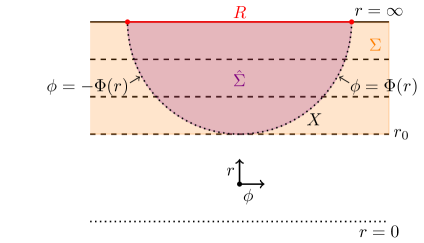
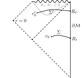
Figure 1: Left: the planar symmetric homology hypersurface $\hat{\Sigma}$ with respect to the HRT surface $X$. $\Sigma$ is the extended homology hypersurface, whose boundary is the plane at $r=r_{0}$. Dashed lines are planes – i.e. constant $r$ surfaces. Right: example conformal diagram indicating possible embeddings of two extended homology hypersurfaces $\Sigma$ and $\Sigma^{\prime}$. The grey line is an apparent horizon, with vanishing outwards null expansion, $\theta_{+}=0$.

Without loss of generality, we will bound the time-derivative at $t=0$ and use the shorthands $X_{t=0}=X$ and $R_{t=0}=R$. Since $R$ is a strip contained in a canonical time slice of Minkowski, and since the ambient spacetime has planar symmetry, there exists a homology hypersurface $\hat{\Sigma}$ of $X$ respecting the planar symmetry – see Figure 1. We can pick coordinates on $\hat{\Sigma}$ so that its induced metric $H_{\alpha\beta}$ reads

$$H_{\mu\nu}\differential y^{\mu}\differential y^{\nu}=B(r)\differential r^{2}+r^{2}(\differential\phi^{2}+\differential\bm{x}^{2}),\quad r\in[r_{0},\infty),\quad\phi\in[-\Phi(r),\Phi(r)],$$ (2.19)

where $\phi=\Phi(r)$ is the coordinate embedding function of (half of) the HRT surface in $\hat{\Sigma}$, as illustrated in Figure 1. $r_{0}$ is the smallest value of $r$ probed by the HRT surface, corresponding to its tip. $\hat{\Sigma}$ can naturally be extended to include all $\phi\in\mathbb{R}$ by planar symmetry, and this choice turns out to be convenient for us. We denote the corresponding hypersurface as $\Sigma$, and refer to it as the extended homology hypersurface. See Figure  1. The boundary of $\Sigma$ (in the bulk proper) is a plane of radius $r_{0}$.

Relying on the formulas derived in the remainder of this section, we prove the following Lemma in appendix A.5:

Lemma 1.

Let $\Sigma$ be the extended homology hypersurface of an HRT surface $X$ anchored at a strip region given by (2.5). Then a single coordinate system of the form

$$\differential s^{2}=B(r)\differential r^{2}+r^{2}\differential\bm{x}^{2}$$ (2.20)

is enough to cover all of $\Sigma$. Furthermore, $X$ has only one turning point, meaning that embedding function $r(\phi)$ is monotonically increasing for $\phi\geq 0$.

This means one function $\Phi(r)$ contains all the information about the embedding of $X$ in $\Sigma$ – we do not need multiple branches. It also means that $\Sigma$ cannot have any locally stationary planes – that is – no planes of vanishing mean curvature, where $B(r)$ would blow up. The means we never need to worry about patching across coordinate systems when working on $\Sigma$. Geometrically, it implies that $\Sigma$ has no “throats”.

Now, taking $(r,\bm{x})$ to be coordinates on $X$, the induced metric on $X$ reads

$$\differential s^{2}|_{X}=\left[B(r)+r^{2}\Phi^{\prime}(r)^{2}\right]\differential r^{2}+r^{2}\differential\bm{x}^{2}.$$ (2.21)

Since $X$ is an extremal surface, its area is stationary under all variations, including under variations within $\Sigma$. Enforcing this gives an ODE for $\Phi(r)$ in terms of $B(r)$. To find it, we compute the mean curvature $\mathcal{K}$ of $X$ viewed as a submanifold of $\Sigma$ and demand it to be zero. This gives the equation (see appendix A.1 for a computation)

$$rB\Phi^{\prime\prime}+(d-1)r^{2}\left(\Phi^{\prime}\right)^{3}+\Phi^{\prime}\left(dB-\frac{r}{2}B^{\prime}\right)=0.$$ (2.22)

The relevant boundary conditions are

$$\Phi^{\prime}(r_{0})=\infty,\quad\Phi(r_{0})=0,$$ (2.23)

where the former says that $r_{0}$ is the radius of the plane tangent to the tip of the HRT surface (i.e. where $\frac{\differential r}{\differential\phi}=0$), while the latter implements that $\phi=0$ corresponds to the center of the strip. It turns out that equation (2.22) can be integrated, and the solution with the correct boundary condition is

$$\Phi(r)=\int_{r_{0}}^{r}\differential\rho\frac{\sqrt{B(\rho)}}{\rho\sqrt{(\rho/r_{0})^{2d-2}-1}}.$$ (2.24)

This gives the location of the HRT surface within $\Sigma$ explicitly in terms of the geometry of $\Sigma$. We now use this solution to determine the Einstein constraint equations on $\Sigma$, and to derive a formula for the rate of change of the entanglement growth.

2.3 A momentum-entanglement correspondence

Since $X_{t}$ is extremal, its first order variation reduces to a pure boundary term given by (see for example the appendix of [96, 95]):

$$\frac{\differential\text{Area}[X_{t}]}{\differential t}\Big{|}_{t=0}=\int_{\partial X}N^{a}\eta_{a},$$ (2.25)

where $\eta^{a}$ is the translation vector generating the flow of $\partial X_{t}$ at conformal infinity at $t=0$, while $N^{a}$ is the normal to $\partial X$ that is also tangent to $X$, and that points towards the conformal boundary. In writing this formula, we implicitly assume that it is evaluated with some near-boundary cutoff that is subsequently removed. As is well known, given some choice of boundary conformal frame, a canonical choice of cutoff exists [97, 98, 99], which in our case reduces to a cutoff in the radial coordinate $r$. With a cutoff adapted to the Minkowski conformal frame and the falloffs (2.3), (2.25) is finite, even though $\text{Area}[X_{t}]$ diverges.

Now we write (2.25) in a more useful form. We will give all the main steps, but relegate tedious but straight forward computations to the appendix.

Using the planar symmetry of $\Sigma$, the extrinsic curvature $K_{\alpha\beta}$ of $\Sigma$ is given by

$$K_{\mu\nu}\differential y^{\mu}\differential y^{\nu}=K_{rr}(r)\differential r^{2}+K_{\phi\phi}(r)\left[\differential\phi^{2}+\differential\bm{x}^{2}\right],$$ (2.26)

where we take the extrinsic curvature to be defined with respect to the future directed normal. Using this, we show in appendix (A.3), retracing the steps of [100], that

$$\frac{\differential\text{Area}[X_{t}]}{\differential t}\Big{|}_{t=0}=-\frac{\text{Area}[\partial R]}{L^{d-2}}\lim_{r\rightarrow\infty}r^{d-3}K_{\phi\phi}.$$ (2.27)

Physically, $\lim_{r\rightarrow\infty}r^{d-3}K_{\phi\phi}$ measures the boost angle at which $X$ hits the conformal boundary, or rather, the subleading part of the angle, since extremality implies that $X$ hits $\partial\mathcal{M}$ orthogonally. This can be seen by studying extremal surfaces in a near-boundary expansion. Thus, we see that the entanglement growth is, up to a factor, identically given by the (subleading) boost angle at which the HRT surface hits the boundary. The same was found for maximal volume slices in [100].

Next we want to find a more explicit expression for $\lim_{r\rightarrow\infty}r^{d-3}K_{\phi\phi}$. To do this, we need to use the Einstein constraint equations, which read

$$\mathcal{R}+K^{2}-K^{\alpha\beta}K_{\alpha\beta}+\frac{d(d-1)}{L^{2}} =16\pi G_{N}\mathcal{T}_{ab}t^{a}t^{b},$$ (2.28)

$$D_{\alpha}K\indices{{}^{\alpha}_{\beta}}-D_{\beta}K =8\pi G_{N}\mathcal{T}_{ab}t^{a}e^{b}_{\beta},$$

where $\mathcal{R}$ is the Ricci scalar of the metric on $\Sigma$, $t^{a}$ the future unit normal to $\Sigma$, $K=H^{\alpha\beta}K_{\alpha\beta}$, and $e^{a}_{\alpha}$ a set of tangent vectors to $\Sigma$. To write these equations in coordinate form, it is convenient to introduce the function $\omega(r)$ as

$$B(r)=\frac{1}{\frac{r^{2}}{L^{2}}-\frac{\omega(r)}{r^{d-2}}}.$$ (2.29)

We will call $\omega(r)$ the Riemannian Hawking mass. It will play a central role in our work. Whether or not $\omega(\infty)$ is proportional to the spacetime mass for some general spacelike hypersurface $\Sigma$ depends on the behavior of the extrinsic curvature $\Sigma$ at large $r$. It turns out that for $d\geq 3$, and with $\Sigma$ being the extended homology hypersurface of an HRT surface, it has the property that it is proportional to the CFT energy density:

$$\left<T_{tt}\right>=\frac{d-1}{16\pi G_{N}L^{d-1}}\omega(\infty),\qquad d\geq 3.$$ (2.30)

For $d=2$, the right hand side is a lower bound on $\left<T_{tt}\right>-\left<T_{tt}\right>_{\rm vac}$, where the vacuum energy must be subtracted when we allow $\phi$ to be periodic. We will explain these facts in Sec. 2.5.

It is also convenient to redefine $K_{rr}(r)$ in terms of a function $F(r)$ which is the $rr$-component of the extrinsic curvature in an orthonormal basis

$$K_{rr}(r)\equiv B(r)F(r).$$ (2.31)

In terms of these functions, the constraint equations in coordinate form read

$$(d-1)\frac{\omega^{\prime}(r)}{r^{d-1}} =2\mathcal{E}(r)-\frac{(d^{2}-3d+2)}{r^{4}}K_{\phi\phi}(r)^{2}-\frac{2(d-1)}{r^{2}}F(r)K_{\phi\phi}(r),$$ (2.32)

$$K_{\phi\phi}^{\prime}(r)-\frac{K_{\phi\phi}(r)}{r} =rF(r)-\frac{r^{2}}{d-1}\mathcal{J}(r),$$ (2.33)

where we introduced the notation

$$\mathcal{E} =8\pi G_{N}\mathcal{T}_{ab}t^{a}t^{b},$$ (2.34)

$$\mathcal{J} =8\pi G_{N}\mathcal{T}_{ab}(\partial_{r})^{a}t^{b}.$$

These are (proportional to) the energy density and radial momentum density of the matter with respect to the frame $t^{a}$. $\mathcal{J}>0$ corresponds to matter falling into the bulk towards smaller $r$. From (2.3) and the fact that $B(r)\sim\mathcal{O}(r^{-1})$, we find that

$$\mathcal{E}\sim o\left(1/r^{d}\right),\qquad\mathcal{J}\sim o\left(1/r^{d+1}\right),$$ (2.35)

where we use that $\frac{1}{\sqrt{B}}(\partial_{r})^{a}$ is a unit vector.

To turn (2.32) and (2.33) into a closed system, we will eliminate $F(r)$. We do this by imposing extremality of $X$ in the direction of $t^{a}$. To do this, note that the inwards (outwards) null expansion $\theta_{+}$ ($\theta_{-}$) of $X$ can be written as (see for example the appendix of [100])

$$\sqrt{2}\theta_{\pm}[X]=\pm\mathcal{K}[X]+K-n^{\alpha}n^{\beta}K_{\alpha\beta},$$ (2.36)

where $n^{\alpha}$ is the outwards normal to $X$ within $\Sigma$, and where we remind that $\mathcal{K}[X]$ is the mean curvature of $X$ within $\Sigma$. Extremality means $\theta_{+}=\theta_{-}=0$, which implies that $\mathcal{K}=0$ and

$$K|_{X}=n^{\alpha}n^{\beta}K_{\alpha\beta}|_{X}.$$ (2.37)

This equation holds at $\phi=\Phi(r)$, which by planar symmetry means it holds everywhere on $\Sigma$. Writing out this equation in coordinates, carried out in appendix A.2, we find

$$F+\frac{({d}-2)K_{\phi\phi}}{r^{2}}+({d}-1)K_{\phi\phi}\frac{(\Phi^{\prime})^{2}}{B}=0.$$ (2.38)

Plugging in the solution for $\Phi(r)$, given in (2.24), we get that

$$F(r)=-\frac{K_{\phi\phi}(r)}{r^{2}}\left(\frac{(d-2)r^{2d-2}+r_{0}^{2d-2}}{r^{2d-2}-r_{0}^{2d-2}}\right),$$ (2.39)

which upon insertion into the constraints, gives a closed system of ODEs

$$\frac{\omega^{\prime}(r)}{r^{d-1}} =\frac{2}{d-1}\mathcal{E}(r)+\frac{K_{\phi\phi}^{2}}{r^{4}}h_{1}(r),$$ (2.40)

$$K_{\phi\phi}^{\prime}(r) +\frac{K_{\phi\phi}}{r}h_{2}(r)=-\frac{r^{2}}{d-1}\mathcal{J}(r),$$ (2.41)

where

$$h_{1}(r)=\frac{(d-2)\left({r}/{r_{0}}\right)^{2d-2}+d}{\left({r}/{r_{0}}\right)^{2d-2}-1},\qquad h_{2}(r)=\frac{(d-3)\left({r}/{r_{0}}\right)^{2d-2}+2}{\left({r}/{r_{0}}\right)^{2d-2}-1}.$$ (2.42)

Now, $F(r)$ is a component of the extrinsic curvature in an orthonormal basis, so it must be finite at $r_{0}$. Using this to fix an integration constant, we find that the solutions of (2.40) and (2.41) are

$$K_{\phi\phi}(r) =-\frac{r^{2}}{(d-1)\sqrt{(r/r_{0})^{2d-2}-1}}\int_{r_{0}}^{r}\differential\rho\mathcal{J}(\rho)\sqrt{(\rho/r_{0})^{2d-2}-1},$$ (2.43)

$$\omega(r) =\omega(r_{0})+\int_{r_{0}}^{r}\differential\rho\left[\rho^{d-5}h_{1}(\rho)K_{\phi\phi}(\rho)^{2}+\frac{2\rho^{d-1}}{d-1}\mathcal{E}(\rho)\right],$$ (2.44)

where $K_{\phi\phi}(r_{0})=0$ since $\mathcal{J}(\rho)$ must be bounded. Inserting (2.43) into (2.27) and multiplying by $(4G_{N})^{-1}$, we get that

$$\frac{\differential S_{R}}{\differential t}\Big{|}_{t=0}=\frac{\text{Area}[\partial R]}{4G_{N}L^{d-2}(d-1)}\int_{r_{0}}^{\infty}\differential r\mathcal{J}(r)\sqrt{r^{2d-2}-r_{0}^{2d-2}}.$$ (2.45)

Since $\mathcal{J}>0$ corresponds to a flux of energy density towards decreasing $r$, we see that matter falling out of the entanglement wedge and deeper into the bulk is directly responsible for the increase of entanglement. Conversely, outgoing matter is responsible for decrease in entanglement. We can also rewrite this formula in a covariant way. In appendix A.3 we show that

$$\frac{\differential S_{R}}{\differential t}\Big{|}_{t=0}=\int_{X}G\mathcal{T}_{ab}n^{a}t^{a}$$ (2.46)

where $n^{a}$ is the outwards unit normal to $X$ that is tangent to $\Sigma$, and

$$G(r)=\frac{2\pi r^{d}}{(d-1)r_{0}^{d-1}}.$$ (2.47)

The formulas (2.27), (2.43)–(2.47) are the main results of this section. These results together with the theorems proven in the following section are crucial pieces to our proven bounds.

2.4 Geometric constraints on the HRT surface

In this section, we prove the following

Theorem 5.

Let $(\mathcal{M},g_{ab})$ be a regular asymptotically AdS_d+1≥3 spacetime with planar symmetry satisfying the DEC. Let $X$ be the HRT surface of a strip $R$ of width $\ell$, and let be $r_{0}$ be the smallest radius probed by $X$. Then

$$\frac{L^{2}}{r_{0}}\leq\frac{\Gamma\left(\frac{1}{2(d-1)}\right)}{2\sqrt{\pi}\Gamma\left(\frac{d}{2(d-1)}\right)}\ell.$$ (2.48)

Furthermore, if $r_{0,\rm vac}$ is the smallest radius probed by the HRT surface $X_{0}$ of a strip of width $\ell$ in pure AdS_d+1, then

$$r_{0}\geq r_{0,{\rm vac}}.$$ (2.49)

We now give the proof assuming that $\omega(r_{0})\geq 0$, and then we will spend most of the rest of this section proving this assertion.

Proof.

By Lemma 3, proven below, we have that $\omega(r_{0})\geq 0$. Furthermore, the DEC implies that $\mathcal{E}$ is positive. Hence, (2.44) gives that $\omega(r)$ is everywhere positive. But this means that

$$B(r)=\frac{1}{\frac{r^{2}}{L^{2}}-\frac{\omega(r)}{r^{d-2}}}\geq\frac{L^{2}}{r^{2}},$$ (2.50)

which allows us to lower bound the strip width as follows:

$$\ell =2L\Phi(\infty)=2L\int_{r_{0}}^{\infty}\differential\rho\frac{\sqrt{B(\rho)}}{\rho\sqrt{(\rho/r_{0})^{2d-2}-1}}$$ (2.51)

$$\geq 2L^{2}\int_{r_{0}}^{\infty}\differential\rho\frac{1}{\rho^{2}\sqrt{(\rho/r_{0})^{2d-2}-1}}$$

$$=\frac{2L^{2}}{r_{0}}\frac{\sqrt{\pi}\Gamma\left(\frac{d}{2(d-1)}\right)}{\Gamma\left(\frac{1}{2(d-1)}\right)}.$$

Finally, if we are in pure AdS, we must have have that the spacetime mass is vanishing, implying that $\omega(\infty)=0$, and so by $\omega^{\prime}(r)\geq 0$ and the fact that $\omega(r_{0})\geq 0$, we must have $\omega(r)=0$ everywhere. But that means that the above inequalities become equalities, giving $\frac{L^{2}}{r_{0}}\geq\frac{L^{2}}{r_{0,\text{vac}}}$, which implies (2.49). ∎

Now we turn to proving that $\omega(r_{0})$ is non-negative. The crucial tool is a planar-symmetric AdS_d+1 version of the Lorentzian Hawking mass [105], which we define for a planar surface $\sigma$ as

$$\mu[\sigma]=\frac{r^{d}}{L^{2}}-\frac{2r^{d}\theta_{+}\theta_{-}}{k_{+}\cdot k_{-}(d-1)^{2}},$$ (2.52)

where $k^{+}$ and $k^{-}$ are the outwards and inwards null vectors orthogonal to $\sigma$, respectively, and $\theta_{\pm}$ the corresponding null expansions. In [106], generalizing the results of [107] to planar symmetry and AAdS_d+1 spacetimes, it was shown that the DEC implies that $\mu[\sigma]$ is monotonically non-decreasing when $\sigma$ is moving in an outwards spacelike direction, provided we are in a normal region of spacetime, meaning that $\theta_{+}\geq 0,\theta_{-}\leq 0$ when we take $k_{+}^{a}$ and $k_{-}^{a}$ to be future directed.

Furthermore, it is useful to rewrite the Riemannian Hawking mass $\omega(r)$ in a different way. $\omega$ can be thought of as a function of a planar surface $\sigma$ together with a hypersurface $\Sigma$ containing it, and in [100] it is shown that we can write $\omega$ as

$$\omega[\sigma,\Sigma]=\frac{r^{d}}{L^{2}}-\frac{\mathcal{K}[\sigma]^{2}}{(d-1)^{2}},$$ (2.53)

where $\mathcal{K}$ is the mean curvature of $\sigma$ in $\Sigma$. Using (2.36), which assumes the normalization $k_{+}\cdot k_{-}=-1$, we see that $2\theta_{+}\theta_{-}=(K-n^{\alpha}n^{\beta}K_{\alpha\beta})^{2}-\mathcal{K}^{2}$, and so we get the following relation between the Hawking masses

$$\mu[\sigma]=\omega[\sigma,\Sigma]+\frac{r^{d}}{(d-1)^{2}}(K-n^{\alpha}n^{\beta}K_{\alpha\beta})^{2}.$$ (2.54)

With this in hand, we prove the following Lemma.

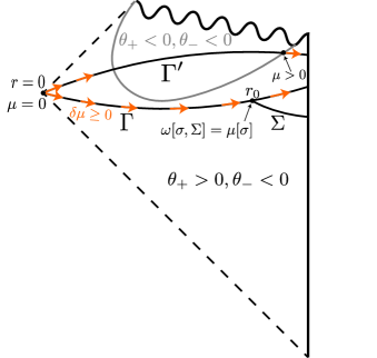
Figure 2: Example of two complete hypersurfaces $\Gamma$ and $\Gamma^{\prime}$. The Lorentzian Hawking mass is vanishing at $r=0$ and positive at marginally trapped surfaces, given by the planes contained in the gray line. $\mu$ is monotonically non-decreasing along spacelike outwards flows in the untrapped region, where $\theta_{+}\geq 0,\theta_{-}\leq 0$. At the boundary $\sigma$ of the extended homology hypersurface $\Sigma$, the Riemannian Hawking mass $\omega$ with respect to $\Sigma$ agrees with the Lorentzian Hawking mass $\mu$.

Lemma 2.

Let $\Gamma$ be a complete planar symmetric hypersurface with one conformal boundary. Let $\sigma_{r}$ be a one-parameter family of planes in $\Gamma$ with radius $r$, and with $r\in(0,\epsilon]$ for any $\epsilon>0$. Then

$$\lim_{r\rightarrow 0}\mu[\sigma_{r}]\geq 0.$$ (2.55)

Proof.

Let us pick coordinates

$$\differential s^{2}|_{\Gamma}=\left[\frac{r^{2}}{L^{2}}-\frac{\omega(r)}{r^{d-2}}\right]^{-1}\differential r^{2}+r^{2}\differential\bm{x}^{2}$$ (2.56)

on $\Gamma$ in a neighborhood of $r=0$. Since $\Gamma$ is complete and we only have one conformal boundary, arbitrarily small $r$ must be part of $\Gamma$. Since $\Gamma$ is spacelike, we must have $\omega(r)\leq r^{d}/L^{2}$, which means that $\omega(r)\sim\mathcal{O}(r^{d})$ at small $r$. Now, from (2.54) we see that $\mu[\sigma_{r}]\geq\omega[\sigma_{r},\Gamma]$ and so

$$\mu[\sigma_{r}]\geq\mathcal{O}(r^{d}).$$ (2.57)

Taking $r\rightarrow 0$ proves our assertion. ∎

Now we are ready to prove that $\omega(r_{0})\geq 0$, together with the fact that the tip of the HRT surface cannot lie in a trapped region.

Lemma 3.

Let $(\mathcal{M},g_{ab})$ be a planar-symmetric regular asymptotically AdS_d+1 spacetime. Let $X$ be the HRT surface of a strip. Then the tip of $X$ lies in an untrapped region of spacetime, meaning the future null expansions of the plane $\sigma$ tangent to $X$ at the tip satisfies

$$\theta_{+}[\sigma]\geq 0,\quad\theta_{-}[\sigma]\leq 0.$$ (2.58)

Furthermore, if the DEC holds and $(\mathcal{M},g)$ is regular, the Riemannian Hawking mass of $\sigma$ is non-negative:

$$\omega[\sigma,\Sigma]=\omega(r_{0})\geq 0.$$ (2.59)

Proof.

Let $\Sigma$ be the unique planar symmetric extended homology hypersurface containing $X$. Let $\sigma$ be the boundary of $\Sigma$ in the bulk, having radius $r_{0}$. Its null expansion is

$$\sqrt{2}\theta_{\pm}[\sigma]=\pm\mathcal{K}[\sigma]+K-r^{\alpha}r^{\beta}K_{\alpha\beta},$$ (2.60)

where $r^{\alpha}=\frac{1}{\sqrt{B}}(\partial_{r})^{\alpha}$. An explicit computation gives

$$\mathcal{K}[\sigma] =\frac{d-1}{r_{0}\sqrt{B(r_{0})}},$$ (2.61)

$$K =\frac{1}{B}K_{rr}+\frac{K_{\phi\phi}(d-1)}{r^{2}},$$

and so we find

$$\sqrt{2}\theta_{\pm}[\sigma]=\pm\frac{d-1}{r_{0}\sqrt{B(r_{0})}}-\frac{K_{\phi\phi}(r_{0})(d-1)}{r_{0}^{2}}.$$ (2.62)

From (2.43) we have that $K_{\phi\phi}(r_{0})=0$, and so we get that

$$\pm\theta_{\pm}\geq 0,$$ (2.63)

proving the first assertion.

Next, since $K_{\phi\phi}(r_{0})=0$ we see that $2\theta_{+}\theta_{-}|_{\sigma}=-\mathcal{K}^{2}|_{\sigma}$, implying that $\mu[\sigma]=\omega[\sigma,\Sigma]$. Now, since our spacetime is AdS-hyperbolic, we can embed $\sigma$ in a complete hypersurface with planar symmetry $\Gamma$, see Figure 2. Since $\sigma$ lies in an untrapped region of spacetime, and since $\Gamma$ is spacelike, $\mu[\sigma]$ is monotonically non-increasing as we deform $\sigma$ in inwards along $\Gamma$ while preserving its planar symmetry. Since the $g_{ab}$ is $C^{2}$, $\theta_{\pm}$ are continuous, and so as we deform $\sigma$ inwards, one of two things happen. Either we hit a marginally trapped surface, where $\theta_{+}\theta_{-}=0$ and where $\mu$ is manifestly positive, or we approach $r=0$, where we again have that $\mu$ is non-negative by Lemma 2. See Figure 2. But since $\mu$ is non-increasing along this deformation, and since it ends up somewhere non-negative, we must have $\mu[\sigma]\geq 0$. But $\mu[\sigma]=\omega[\sigma,\Sigma]$, completing the proof. ∎

We have illustrated the fact that the tip cannot lie in a trapped region of spacetime in Figure 1 – the tip cannot lie behind the gray line. Note that the proof of this fact does not rely on the DEC. This result improves on the findings of [109] in the special case where we have planar symmetry. In [109], they showed without any symmetry assumptions that the tip of an HRT surface in a $(2+1)$–dimensional spacetime can never lie in the so-called umbral region, which is a special subset of the trapped region that lies behind regular holographic screens [110, 109]. They also showed this result with planar symmetry in all dimensions. Here we extend this result to show that the whole trapped region is forbidden, although our result is more limited in that it always requires planar symmetry and a strip (or spherical) boundary region. Note also that this result does not forbid $X$ to probe inside trapped regions – it is only the tip that is forbidden to lie there (see Figure 1). For example, for early times after a quench, the HRT surface will have portions threading through the trapped region [33, 34].

2.5 Proofs

Proof of $d=2$ bound

We are now ready to prove Theorem 1. Evaluating the Lorentzian Hawking mass on a sphere at large $r$ in a planar symmetric AAdS_d+1 spacetime with falloffs (2.3), we get that

$$\left<T_{tt}\right>=\frac{d-1}{16\pi G_{N}L^{d-1}}\mu(\infty).$$ (2.64)

This is valid also for $d=2$, except if $\phi$ is periodically identified, we must replace the left hand side with $\left<T_{tt}\right>-\left<T_{tt}\right>_{\rm vac}$. It can be seen to be true by evaluating $\mu(\infty)$ near the boundary in the usual Fefferman-Graham expansion [97, 98, 99]. Now, from (2.54) and (2.61) we have that

$$\mu(r)=\omega(r)+r^{d-4}K_{\phi\phi}(r)^{2}.$$ (2.65)

From (2.43), we see that $K_{\phi\phi}$ has asymptotic falloff $K_{\phi\phi}\sim\mathcal{O}(r^{3-d})$. Thus, we get that for $d\geq 3$, $\mu(\infty)=\omega(\infty)$, while for $d=2$, we have

$$\mu(\infty)=\omega(\infty)+\left(\lim_{r\rightarrow\infty}r^{-1}K_{\phi\phi}\right)^{2}.$$ (2.66)

Since $\omega(\infty)\geq 0$ by the DEC, when $d=2$ we obtain

$$\Big{|}\lim_{r\rightarrow\infty}r^{-1}K_{\phi\phi}\Big{|}\leq\sqrt{\mu(\infty)}=\sqrt{16\pi G_{N}L\left<T_{tt}\right>}.$$ (2.67)

Using that $\text{Area}[\partial R_{t}]=2$, and combining (2.67) and (2.27) then yields

$$\Big{|}\frac{\differential S_{R}}{\differential t}\Big{|}_{t=0} \leq\frac{1}{2G_{N}}\sqrt{16\pi G_{N}L\left<T_{tt}\right>}=\sqrt{\frac{8\pi c}{3}\left<T_{tt}\right>},$$ (2.68)

where we used the known Brown-Henneaux expression for the central charge: $c=\frac{3L}{2G_{N}}$ [111]. This proves Theorem 1.

Proof of bound for small $\ell$

Now let us consider the result for small subregions, given by Theorem 3. The following Lemma is what we need:

Lemma 4.

Let $(\mathcal{M},g_{ab})$ be a regular asymptotically AdS_d+1≥3 spacetime with planar symmetry satisfying the DEC. Let $X$ be the HRT surface of a strip $R$ of width $\ell$, and let be $r_{0}$ be the smallest radius probed by $X$. Assume that

$$\frac{\ell^{d}\left<T_{tt}\right>}{c_{\rm eff}}\ll 1.$$ (2.69)

Then

$$\Big{|}\lim_{r\rightarrow\infty}r^{d-3}K_{\phi\phi}\Big{|}\leq\frac{L}{2r_{0}}\omega(\infty)\left[1+\mathcal{O}\left(\frac{\ell^{d}\left<T_{tt}\right>}{c_{\rm eff}}\right)\right].$$ (2.70)

Proof.

Let us for convenience define $W=-\lim_{r\rightarrow\infty}r^{d-3}K_{\phi\phi}$, and assume without loss of generality that $W>0$ (otherwise, just reverse the time direction). Using the solutions (2.43) and (2.44), we have that

$$\frac{W}{\omega(\infty)} =\frac{1}{d-1}\frac{\int_{r_{0}}^{\infty}\differential r\mathcal{J}(r)\sqrt{r^{2d-2}-r_{0}^{2d-2}}}{\omega(r_{0})+\int_{r_{0}}^{\infty}\differential r\left[r^{d-5}h_{1}(r)K_{\phi\phi}(r)^{2}+\frac{2r^{d-1}}{d-1}\mathcal{E}(r)\right]}$$ (2.71)

$$\leq\frac{\int_{r_{0}}^{\infty}\differential rr^{d-1}\mathcal{J}(r)}{2\int_{r_{0}}^{\infty}\differential rr^{d-1}\mathcal{E}(\rho)}.$$

The DEC requires that

$$0\leq 8\pi G_{N}\mathcal{T}_{ab}\left[t^{a}\pm\frac{1}{\sqrt{B}}(\partial_{r})^{a}\right]t^{b}=\mathcal{E}\pm\frac{1}{\sqrt{B}}\mathcal{J},$$ (2.72)

and so we have that

$$\mathcal{E}\geq\frac{1}{\sqrt{B}}|\mathcal{J}|.$$ (2.73)

Writing $B$ in terms of $\omega$, and enforcing the DEC, we get

$$\frac{W}{\omega(\infty)} \leq\frac{\int_{r_{0}}^{\infty}\differential rr^{d-1}\mathcal{J}(r)}{\frac{2}{L}\int_{r_{0}}^{\infty}\differential rr^{d}\sqrt{1-\frac{\omega(r)L^{2}}{r^{d}}}|\mathcal{J}(r)|}.$$ (2.74)

Let us now for a moment assume that we are perturbatively close to the vacuum, where $\mathcal{\epsilon}$ is a perturbative parameter parametrizing the magnitude of $\omega(\infty)$. By monotonicity and positivity of $\omega(r)$, $\omega(r)\sim\mathcal{O}(\epsilon)$ as well, and so the $\omega(r)$ appearing in the square root gives higher order contributions:

$$\frac{W}{\omega(\infty)} \leq\frac{\int_{r_{0}}^{\infty}\differential rr^{d-1}|\mathcal{J}(r)|}{\frac{2}{L}\left[\int_{r_{0}}^{\infty}\differential rr^{d}|\mathcal{J}(r)|-\frac{L^{2}}{2}\int_{r_{0}}^{\infty}\differential r\omega(r)|\mathcal{J}(r)|+\ldots\right]}$$ (2.75)

$$=\frac{L}{2}\frac{\int_{r_{0}}^{\infty}\differential rr^{d-1}|\mathcal{J}(r)|}{\int_{r_{0}}^{\infty}\differential rr^{d}|\mathcal{J}(r)|}\left[1+\frac{L^{2}}{2}\frac{\int_{r_{0}}^{\infty}\differential r\omega(r)|\mathcal{J}|}{\int_{r_{0}}^{\infty}\differential rr^{d}|\mathcal{J}|}+\ldots\right]$$

$$\leq\frac{L}{2r_{0}}\left[1+\frac{L^{2}}{r_{0}^{d}}\omega(\infty)+\ldots\right]$$

$$\leq\frac{L}{2r_{0}}\left[1+\frac{L^{2d}}{r_{0}^{d}}\frac{\mu(\infty)}{L^{2d-2}}+\ldots\right]$$

$$=\frac{L}{2r_{0}}\left[1+\frac{16\pi\eta_{d}}{d-1}\frac{\ell^{d}\left<T_{tt}\right>}{c_{\rm eff}}+\ldots\right]$$

where $\eta_{d}$ is the $O(1)$ number coming from using (2.48). We see that the effective expansion parameter is the dimensionless quantity $\frac{\ell^{d}\left<T_{tt}\right>}{c_{\rm eff}}$. So the expansion is not really in small mass, which is dimensionful, but in small strip width relative to the inverse energy density per CFT degree of freedom. ∎

From (2.27) and (2.48), we get, up to the perturbative corrections,

$$\Big{|}\frac{\differential S_{R}}{\differential t}\Big{|} \leq\frac{\text{Area}[\partial R]}{4G_{N}L^{d-2}}\frac{L}{2r_{0}}\omega(\infty)\leq\frac{\sqrt{\pi}}{d-1}\frac{\Gamma\left(\frac{1}{2(d-1)}\right)}{\Gamma\left(\frac{d}{2(d-1)}\right)}\ell\text{Area}[\partial R]\left<T_{tt}\right>$$ (2.76)

$$=\text{Vol}[R]\left<T_{tt}\right>\begin{cases}2\pi&d=2\\ \frac{\sqrt{\pi}}{d-1}\frac{\Gamma\left(\frac{1}{2(d-1)}\right)}{\Gamma\left(\frac{d}{2(d-1)}\right)}&d>2\end{cases},$$

where we used (2.48) and (2.30) in the second inequality. This also holds for $d=2$, since $\omega(\infty)\leq\mu(\infty)$, provided we replace $\left<T_{tt}\right>\rightarrow\left<T_{tt}\right>-\left<T_{tt}\right>_{\rm vac}$ if $\phi$ is compact. Also, note that for $d=2$ we have that $\ell\text{Area}[\partial R]=2\text{Vol}[R]$. This completes the proof of Theorem 3 for strip regions.

Proof of bounds in thin-shell spacetimes

We now turn our attention to thin-shell spacetimes, where we will be able to establish that a bound of the form $|\partial_{t}S|\leq\#\text{Vol}[R]\left<T_{tt}\right>$ holds for any $\ell$. Furthermore, in this class of spacetimes we will prove our conjectured generalization of Theorem 1 to $d>2$, i.e. Theorem 2.

Figure 3: Examples of thin-shell spacetimes, where the blue lines correspond to the shells. The left space is dual to a uniform quench, where matter is thrown in from the boundary, while the right is a spacetime with a brane in the bulk interior.

Consider a spacetime where the matter consists of a single thin shell of matter that separately satisfies the DEC, together with a possible contribution from any number of $U(1)$ gauge fields:

$$\mathcal{E} =\kappa\delta(r-\hat{r})+\mathcal{E}^{\rm Maxwell},$$ (2.77)

$$\mathcal{J} =\eta\delta(r-\hat{r}),$$

for some $\eta,\kappa,\hat{r}>r_{0}$. See Figure 3. Here we used that in planar symmetry, Maxwell fields give no contribution to the radial momentum density $\mathcal{J}$ (see for example Sec. 3 of [100]). In fact, we can add to the $U(1)$ gauge fields any matter that has a positive contribution to $\mathcal{E}$ but no contribution to $\mathcal{J}$.

The DEC, through (2.73), imposes that $\mathcal{J}$ only can have support at $\hat{r}$. Without loss of generality, we take $\eta>0$. Let us in this section also use our scaling freedom in $r$ to set $r_{0}=L$ and choice of units to set $L=1$.

Define again $W=-\lim_{r\rightarrow\infty}r^{d-3}K_{\phi\phi}$. Plugging (2.77) into (2.43), the solution for $K_{\phi\phi}$ is

$$K_{\phi\phi}(r) =-\frac{r^{2}}{d-1}\eta\sqrt{\frac{\hat{r}^{2d-2}-1}{r^{2d-2}-1}}\theta(r-\hat{r}),$$ (2.78)

and so

$$\eta=\frac{(d-1)W}{\sqrt{\hat{r}^{2d-2}-1}},$$ (2.79)

which gives

$$K_{\phi\phi}(r)=-\frac{r^{2}W}{\sqrt{r^{2d-2}-1}}\theta(r-\hat{r}).$$ (2.80)

Next, let us solve for the contribution to $\omega(r)$ from the squared extrinsic curvature term in (2.44):

$$Q(r) \equiv\int_{1}^{r}\differential\rho\rho^{d-5}K_{\phi\phi}(\rho)^{2}h_{1}(\rho)$$ (2.81)

$$=\theta(r-\hat{r})W^{2}\int_{\hat{r}}^{r}\differential\rho\rho^{d-1}\frac{h_{1}(\rho)}{\left[\rho^{2d-2}-1\right]}$$

$$=W^{2}\theta(r-\hat{r})\left[\frac{\hat{r}^{d}}{\hat{r}^{2d-2}-1}-\frac{r^{d}}{r^{2d-2}-1}\right].$$

To proceed, we need to understand what happens to $\omega$ as we cross the shock. Restricting attention to a small neighborhood of $\hat{r}$, where we can treat explicit occurrences of $r$ not appearing in delta functions as constant, the equation for $\omega$ reads

$$(d-1)\frac{\omega^{\prime}(r)}{\hat{r}^{d-1}}=2\mathcal{E}^{\rm shell}+\ldots,$$ (2.82)

where the terms indicated with dots will make no contribution to the discontinuity. Remembering that the DEC implies that $\sqrt{B}\mathcal{E}\geq|\mathcal{J}|$, imposing the DEC on the shell means that

$$\mathcal{E}^{\rm shell}\geq\sqrt{\hat{r}^{2}-\frac{\omega(r)}{\hat{r}^{d-2}}}\eta\delta(r-\hat{r}).$$ (2.83)

Inserting (2.83) into (2.82), dividing by the prefactor of the delta function, and integrating from $\hat{r}-\varepsilon$ to $\hat{r}+\varepsilon$ for some small positive $\varepsilon$, we find

$$\sqrt{\hat{r}^{2}-\frac{\omega_{-}}{\hat{r}^{d-2}}}-\sqrt{\hat{r}^{2}-\frac{\omega_{+}}{\hat{r}^{d-2}}}\geq\frac{\hat{r}}{d-1}\eta+\mathcal{O}(\varepsilon),$$ (2.84)

where we defined $\omega_{\pm}=\omega(\hat{r}\pm\varepsilon)$. We only have a sensible solution when $B(r)$ is real and positive everywhere, which requires

$$\frac{1}{d-1}\eta\leq\sqrt{1-\frac{\omega_{-}}{\hat{r}^{d}}}.$$ (2.85)

Solving for $\omega_{-}$ from (2.84) and inserting our expression for $\eta$, we get that

$$\omega_{+} \geq\omega_{-}+\frac{\hat{r}^{d}}{\sqrt{\hat{r}^{2d-2}-1}}W\left[\sqrt{1-\frac{\omega_{-}}{\hat{r}^{d}}}-\frac{W}{\sqrt{\hat{r}^{2d-2}-1}}\right].$$ (2.86)

Using this and (2.65), the Lorentzian Hawking mass at infinity has the lower bound

$$\mu(\infty) =\omega(\infty)+\delta_{d2}W^{2}$$ (2.87)

$$\geq\omega_{-}+\frac{\hat{r}^{d}}{\sqrt{\hat{r}^{2d-2}-1}}W\left[\sqrt{1-\frac{\omega_{-}}{\hat{r}^{d}}}-\frac{W}{\sqrt{\hat{r}^{2d-2}-1}}\right]+Q(\infty)+\delta_{d2}W^{2}$$

$$=\omega_{-}+\frac{\hat{r}^{d}}{\sqrt{\hat{r}^{2d-2}-1}}W\sqrt{1-\frac{\omega_{-}}{\hat{r}^{d}}},$$

where $\delta_{ij}$ is the Kronecker delta. Thus, for any real $n$, we have that

$$\frac{W^{n}}{\mu(\infty)}\leq\frac{W^{n}}{\omega_{-}+\frac{\hat{r}^{d}}{\sqrt{\hat{r}^{2d-2}-1}}W\sqrt{1-\frac{\omega_{-}}{\hat{r}^{d}}}}\equiv U_{n},$$ (2.88)

together with the constraints

$$0 \leq\omega_{-}\leq\hat{r}^{d},$$ (2.89)

$$W \leq\sqrt{\hat{r}^{2d-2}-1}\sqrt{1-\frac{\omega_{-}}{\hat{r}^{d}}}.$$ (2.90)

Our goal will now be to upper bound $U_{n}$ for all legal triplets $\left(W,\hat{r},\omega_{-}\right)$ for $n=1$ and $n=\frac{d}{d-1}$, which turns out to be values that will give interesting growth bounds.

Note first that we have

$$\partial_{\omega_{-}}^{2}U_{n}\geq 0,$$ (2.91)

so any local extremum of $U_{n}$ with respect to $\omega_{-}$ is a minimum. Thus, for any given $W$ and $\hat{r}$, $U_{n}$ is maximized when $\omega_{-}$ is on the boundary of its domain. First, take $\omega_{-}=0$. Then, assuming that $1\leq n\leq\frac{d}{d-1}$,

$$U_{n}=\frac{W^{n-1}\sqrt{\hat{r}^{2d-2}-1}}{\hat{r}^{d}}\leq\frac{\left[\hat{r}^{2d-2}-1\right]^{\frac{n}{2}}}{\hat{r}^{d}}\leq\frac{\hat{r}^{n(d-1)}}{\hat{r}^{d}}\leq 1,$$ (2.92)

where we used (2.90) in the second inequality. For $n=1$, we get the stronger bound

$$U_{1}\leq\frac{\sqrt{\hat{r}^{2d-2}-1}}{\hat{r}^{d}}\leq\sqrt{\frac{d-1}{d^{\frac{d}{d-1}}}}\equiv\alpha_{d},$$ (2.93)

where the upper bound is found by maximizing with respect to $\hat{r}$. Next, let us look at the maximal value for $\omega_{-}$, where we have the equality

$$W=\sqrt{\hat{r}^{2d-2}-1}\sqrt{1-\frac{\omega_{-}}{\hat{r}^{d}}}.$$ (2.94)

Neglecting the first $\omega_{-}$ in the denominator of $U_{n}$ and using $W\leq\sqrt{\hat{r}^{2d-2}-1}$, we get

$$U_{n}\leq\frac{\left[\hat{r}^{2d-2}-1\right]^{n/2}}{\hat{r}^{d}}.$$ (2.95)

But this is just the expression bounded earlier, and so (2.92) and (2.93) holds generally. Restoring factors of $L,r_{0}$, we have the following true bounds

$$W \leq L^{\frac{d-2}{d}}\omega(\infty)^{\frac{d-1}{d}},$$ (2.96)

$$W \leq\alpha_{d}\frac{L}{r_{0}}\omega(\infty).$$ (2.97)

Redoing the steps in (2.76) with the numerical factor from in (2.97), we get Theorem 4 for strip regions. Next, inserting (2.96) into (2.27), we find

$$\Big{|}\frac{\differential S_{R}}{\differential t}\Big{|} \leq\frac{\text{Area}[\partial R]}{4G_{N}L^{d-2}}L^{\frac{d-2}{d}}\left[\frac{16\pi G_{N}L^{d-1}}{d-1}\left<T_{tt}\right>\right]^{\frac{d-1}{d}}=\frac{1}{4}\text{Area}[\partial R]c_{\rm eff}\left[\frac{16\pi}{(d-1)c_{\rm eff}}\left<T_{tt}\right>\right]^{\frac{d-1}{d}},$$ (2.98)

proving Theorem 2 for strip regions.

2.6 Multiple strips and mutual information

Our results not scaling with $\text{Vol}[R]$ can be generalized to regions $R$ consisting of $n$ disjoint finite strips by simply applying the same argument to each connected component of the HRT surface separately. For $d=2$ this results in

$$\quantity|\frac{\differential S_{R}}{\differential t}|\leq n\sqrt{\frac{8\pi c}{3}\left<T_{tt}\right>}.$$ (2.99)

It is easy to see that (2.98) also holds true for $n$ strips. No modification is needed, since $\text{Area}[\partial R]$ implicitly contains the factor of $n$ present in the $d=2$ case.

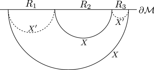
Figure 4: Possible HRT surfaces $X$ and $X^{\prime}$ of the region $R_{1}\cup R_{3}$, projected onto a timeslice.

For the bounds scaling like volume, the behavior is different, since the upper bound depends on the connectivity properties of the entanglement wedge. Consider for example $d=2$ and the three intervals $R_{1},R_{2},R_{3}$ in Figure 4, and let $R=R_{1}\cup R_{3}$ be the region under consideration. We then see that

$$\Big{|}\frac{\differential S_{R}}{\differential t}\Big{|}\leq\kappa\left<T_{tt}\right>\begin{cases}\text{Vol}[R]&\text{the entanglement wedge is disconnected},\\ \text{Vol}[R]+2\text{Vol}[R_{2}]&\text{the entanglement wedge is connected},\\ \end{cases}$$ (2.100)

where $\kappa$ is the relevant numerical prefactor of either Theorem 3 or 4. We get this result by adding the different volume factors from each connected component of the HRT surface. Similar games can be played for $n$ strips in $d$ dimensions.

Next, lets us consider $d=2$ and the mutual information between two subsystems $R_{1}$ and $R_{2}$ consisting of $n_{1}$ and $n_{2}$ finite intervals, respectively. We then have

$$\Big{|}\partial_{t}I(R_{1},R_{2})\Big{|} =|\partial_{t}S_{R_{1}}+\partial_{t}S_{R_{2}}-\partial_{t}S_{R_{1}R_{2}}|\leq|\partial_{t}S_{R_{1}}|+|\partial_{t}S_{R_{2}}|+|\partial_{t}S_{R_{1}R_{2}}|$$ (2.101)

$$\leq\left(2n_{1}+2n_{2}\right)\sqrt{\frac{8\pi c}{3}\left<T_{tt}\right>}.$$

Using (2.12), the generalization to higher $d$ is obvious.

3 Maximal Rates for Balls, Wilson Loops and Correlators

3.1 Setup and summary of results

In this section we will consider extremal surfaces $X_{t}$ of dimension $q+1$ anchored at $q$-dimensional spheres $\partial R_{t}$ at time $t$ on the conformal boundary, where extremal means that all the mean curvatures of $X_{t}$ are zero. We take the spheres to have radius $\mathcal{R}$. For $q=0$, $\partial R_{t}$ just consists of two points, and $X_{t}$ is a one-parameter family of geodesics. For $q=d-2$, $X_{t}$ is a one-parameter family of HRT surfaces anchored at spheres. For $q=1$, $X_{t}$ are two-dimensional spacelike worldsheets anchored at circles.

As before we are working with planar symmetric spacetimes, subject to the same assumptions described in Sec. 2.1. The logical steps will be mostly identical to Sec. 2, but with extra technicalities coming from the curvature of $\partial R_{t}$. Note that since we now have submanifolds of varying dimensions, we will use the symbol $\norm{\cdot}$ to indicate the measure of the surface in the natural induced volume form. For quantities on the conformal boundary, $\norm{\cdot}$ means with respect to the induced metric from the Minkowski conformal frame. We will use $\text{Length}[]$, $\text{Area}[]$ and $\text{Vol}[]$ to refer to the measure of surfaces of dimension 1, codimension 2, and codimension 1, respectively.

To describe the relevant subregions in our results, let $\bm{z}$ be Cartesian coordinates in the direction transverse to the sphere $\partial R_{t}$. We now choose coordinates for our Minkowski conformal frame on the boundary to be

$$\differential s^{2}=-\differential t^{2}+L^{2}\left(\differential\phi^{2}+\phi^{2}\differential\Omega^{2}_{q}+\differential\bm{z}^{2}\right),$$ (3.1)

with $\differential\Omega^{2}_{q}$ the metric of a round unit $q$-sphere, and with the constant$-t$ slices the ones on which one-point functions of local operators are constant. For $q=0$ there is no $\differential\Omega^{2}_{q}$–term, while for $q=d-2$ there is no $\differential\bm{z}^{2}$ term. $\phi$ is a dimensionless radial coordinate on the boundary, and $R_{t^{\prime}}$ is given by

$$0\leq\phi\leq\frac{\mathcal{R}}{L},\qquad t=t^{\prime},\qquad\bm{z}=0.$$ (3.2)

We now have

$$\norm{\partial R_{t}}=\norm{\partial R}=\Omega_{q}\mathcal{R}^{q},$$ (3.3)

where $\Omega_{q}$ is the volume of a unit $q$-sphere.

Let us now summarize the results proven in this section. For entanglement entropy, we will prove the parts Theorems 2, 3 and 4 that refer to spherical $\partial R$. For extremal surfaces of other dimensionalities, the following theorem applies to the most general class of spacetimes and subregions:

Theorem 6.

Let $(\mathcal{M},g_{ab})$ be a regular asymptotically AdS_d+1 spacetime with planar symmetry satisfying the DEC. Assume that $d$ is even, and let be $X_{t}$ be an extremal surface of dimension $d/2$, anchored on the conformal boundary at the sphere $\partial R_{t}$. Then

$$\quantity|\frac{\differential}{\differential t}\norm{X_{t}}|\leq\norm{\partial R}L^{\frac{d}{2}}\sqrt{\frac{16\pi}{c_{\rm eff}(d-1)}\left<T_{tt}\right>}.$$ (3.4)

Of course, for $d=2$, this just reduces to Theorem 1. For $d=4$ this can be converted to the growth bound on circular Wilson loops, given by (1.13). Next, for surfaces $X_{t}$ anchored at small spheres on the boundary, we get the following:

Theorem 7.

Let $(\mathcal{M},g_{ab})$ be a regular asymptotically AdS_d+1 spacetime with planar symmetry satisfying the DEC. Let be $X_{t}$ be an extremal surface of dimension $q+1$, anchored on the conformal boundary at the sphere $\partial R_{t}$ having radius $\mathcal{R}$. Assume that

$$q\geq\frac{d-2}{2}$$ (3.5)

and

$$\frac{\mathcal{R}^{d}\left<T_{tt}\right>}{c_{\rm eff}}\ll 1.$$ (3.6)

Then

$$\quantity|\frac{\differential}{\differential t}\norm{X_{t}}|\leq\eta_{d,q}\norm{\partial R}L^{q+1}\mathcal{R}^{d-q-1}\frac{\left<T_{tt}\right>}{c_{\rm eff}}\left[1+\mathcal{O}\left(\frac{\mathcal{R}^{d}\left<T_{tt}\right>}{c_{\rm eff}}\right)\right],$$ (3.7)

where

$$\eta_{d,q}=\frac{8\pi}{d-1}\left[\frac{\Gamma\left(\frac{1}{2(q+1)}\right)}{\sqrt{\pi}\Gamma\left(\frac{q+2}{2(q+1)}\right)}\right]^{d-q-1}.$$ (3.8)

Using well known dictionary entries, described in Sec. 3.6, this converts to growth bounds on the entanglement of small balls, small circular Wilson loops, and heavy two-point functions at small separations. Specifically, for the latter two, we get

$$\Big{|}\frac{\differential}{\differential t}\log|\left<O(x)O(0)\right>_{\rho(t)}|\Big{|} \leq\frac{8\pi\Delta}{c_{\rm eff}}|x|\left<T_{tt}\right>\left[1+\mathcal{O}\left(\frac{|x|^{2}\left<T_{tt}\right>}{c_{\rm eff}}\right)\right],\quad d=2,$$ (3.9)

and

$$\Big{|}\frac{\differential}{\differential t}\log|\left<\mathcal{W}(C)\right>_{\rho(t)}|\Big{|} \leq\frac{8\pi\sqrt{\lambda_{\rm eff}}}{(d-1)c_{\rm eff}}\eta_{d,1}\mathcal{R}^{d-1}\left<T_{tt}\right>\left[1+\mathcal{O}\left(\frac{\mathcal{R}^{d}\left<T_{tt}\right>}{c_{\rm eff}}\right)\right],\quad d\in\{3,4\},$$ (3.10)

where $\sqrt{\lambda_{\rm eff}}=L^{2}/\ell_{\rm string}^{2}$ is the effective ’t Hooft coupling, and $\ell_{\rm string}$ the bulk string length. Finally, for thin-shell spacetimes, we prove the following:

Theorem 8.

Let $(\mathcal{M},g_{ab})$ be an asymptotically AdS_d+1 spacetime with planar symmetry satisfying the DEC. Assume that $X_{t}$ is an extremal surface anchored at a boundary sphere of dimension

$$q\geq\frac{d-2}{2}.$$ (3.11)

Next, assume that the bulk matter consists of $U(1)$ gauge fields and a thin shell of matter:

$$\mathcal{T}_{ab}=\mathcal{T}_{ab}^{\rm shell}+\mathcal{T}_{ab}^{\rm Maxwell},$$ (3.12)

where $\mathcal{T}_{ab}^{\rm shell}$ has delta function support on a codimension$-1$ worldvolume that is timelike or null, and that separately satisfies the DEC. Assume $(\mathcal{M},g)$ is regular, except we do not require $g_{ab}$ to be $C^{2}$ at the shell. Then

$$\Big{|}\frac{\differential}{\differential t}\norm{X_{t}}\Big{|} \leq\norm{\partial R}L^{q+1}\left[\frac{16\pi}{(d-1)c_{\rm eff}}\left<T_{tt}\right>\right]^{\frac{q+1}{d}}$$ (3.13)

and

$$\quantity|\frac{\differential}{\differential t}\norm{X_{t}}|\leq\kappa_{d,q}\norm{\partial R}L^{q+1}\mathcal{R}^{d-q-1}\frac{\left<T_{tt}\right>}{c_{\rm eff}}$$ (3.14)

with $\kappa_{d,q}$ given by (3.75).

The main application of (3.13) is to bound Wilson loops in $d=3$, where we get

$$\Big{|}\frac{\differential}{\differential t}\log|\left<\mathcal{W}(C)\right>_{\rho(t)}|\Big{|} \leq\frac{\sqrt{\lambda_{\rm eff}}\text{Length}[C]}{2\pi}\left[\frac{8\pi}{c_{\rm eff}}\left<T_{tt}\right>\right]^{2/3}.$$ (3.15)

Let us now turn to the proofs.

3.2 An implicit solution for the extremal surface location

As earlier, let $\Sigma$ be the extended planar symmetric homology hypersurface containing $X$. For the exact same reason as earlier, there is a unique choice of $\Sigma$. We can now pick coordinates on $\Sigma$ given by

$$\differential s^{2}|_{\Sigma}=H_{\mu\nu}\differential y^{\mu}\differential y^{\nu}=B(r)\differential r^{2}+r^{2}\left(\differential\phi^{2}+\phi^{2}\differential\Omega_{q}^{2}+\differential\bm{z}^{2}\right).$$ (3.16)

Again, one such coordinate system covers all of $\Sigma$, as shown in appendix A.5.

We take our intrinsic coordinates on $X$ to be $(r,\Omega^{i})$, where $\Omega^{i}$ are coordinates on the sphere. The embedding coordinates of $X$ in $\Sigma$ reads

$$X^{\mu}=(r,\phi=\Phi(r),\Omega^{i},\bm{z}=0),$$ (3.17)

where the symmetries of the problem dictate $\bm{z}=0$. The induced metric on $X$ is

$$\differential s^{2}|_{X}=\left[B(r)+r^{2}\Phi^{\prime}(r)^{2}\right]\differential r^{2}+r^{2}\Phi(r)^{2}\differential\Omega_{q}^{2}.$$ (3.18)

Now we must implement the condition that $X$ is extremal, which requires us to compute all its mean curvatures and demand them to be vanishing. To do this, let $n_{a}^{I}$ be an orthonormal basis of normal forms to $X$ that are tangent to $\Sigma$, labeled by $I$. Let $t_{a}$ be the future timelike normal orthogonal to $\Sigma$. A complete basis of mean curvatures of $X$ now is

$$\mathcal{K}^{I} =h^{ab}\nabla_{a}n_{b}^{I},$$ (3.19)

$$\mathcal{K}^{0} =h^{ab}\nabla_{a}t_{b},$$

where $h^{ab}=g^{ab}+t^{a}t^{b}-\delta^{IJ}n^{a}_{I}n_{J}^{b}$. All of these quantities must vanish. Considering the $\mathcal{K}^{I}$ corresponding the $\bm{z}$ directions, we just get $0$ by our symmetries. Letting $I=n$ denote the remaining normal direction in $\Sigma$, we get by direct computation that (see appendix (A.6) for some of the required ingredients)

$$\mathcal{K}^{n}=\frac{1}{r\sqrt{B}\left[B+r^{2}(\Phi^{\prime})^{2}\right]^{3/2}}\Bigg{[} r^{2}B\Phi^{\prime\prime}+(q+1)r^{3}(\Phi^{\prime})^{3}$$ (3.20)

$$+\left((q+2)B-\frac{1}{2}rB^{\prime}\right)r\Phi^{\prime}-\frac{qB}{\Phi}\left(B+r^{2}(\Phi^{\prime})^{2}\right)\Bigg{]}.$$

If it was not for the last term, we would reproduce (2.22) by setting $q=d-2$. The new term is caused by the curvature of $\partial R$. Now, with this last term, we no longer have an explicit analytical solution (when $q>0$). However, we can find an implicit solution that lets us proceed. Define

$$\chi(r)=\frac{qB}{\Phi\Phi^{\prime}}\left(\frac{B}{\Phi^{\prime 2}}+r^{2}\right),$$ (3.21)

so that our equation for extremality reads

$$(q+1)r^{3}(\Phi^{\prime})^{3}+\left((q+2)B-\frac{1}{2}rB^{\prime}\right)r\Phi^{\prime}+r^{2}B\Phi^{\prime\prime}-(\Phi^{\prime})^{3}\chi(r)=0.$$ (3.22)

Imposing $\Phi(r_{0})=0$, where $r_{0}$ is the tip of the extremal surface, we have the implicit solution

$$\Phi(r)=\int_{r_{0}}^{r}\differential\rho\frac{\sqrt{B(\rho)}}{\rho\sqrt{\mathcal{C}\rho^{2q+2}h(\rho)-1}},$$ (3.23)

where

$$h(r)=1-\frac{2}{\mathcal{C}}\int_{r_{0}}^{r}\differential\rho\chi(\rho)\rho^{-6-2q},$$ (3.24)

for some $\mathcal{C}$ that is fixed by imposing $\Phi^{\prime}(r_{0})=\infty$. Assuming $h(r_{0})$ is finite, we get that $\mathcal{C}=r_{0}^{-2q-2}$. This is indeed correct, even though $\chi(r_{0})$ looks superficially divergent. Since we are near a minimum of $r(\Phi)$ we have that $r=r_{0}+\mathcal{O}(\Phi^{2})$ near $r_{0}$, and so for $r$ close to $r_{0}$ we get $\Phi=\alpha\sqrt{r-r_{0}}$ for some $\alpha$. Even though $\Phi$ goes to zero at $r_{0}$ we find that

$$\chi(r)\sim\mathcal{O}(1)$$ (3.25)

near $r_{0}$, and so $h(r_{0})=1$. Next, reality of $\Phi(r)$ demands that $h(\rho)\geq(r_{0}/r)^{2q+2}$, while positivity of $\Phi$ and $\Phi^{\prime}$ ensures that $h(r)\leq 1$, and so in total we know that

$$\Phi(r) =\int_{r_{0}}^{r}\differential\rho\frac{\sqrt{B(\rho)}}{\rho\sqrt{(\rho/r_{0})^{2q+2}h(\rho)-1}},\qquad 0<(r_{0}/r)^{2q+2}<h(r)\leq 1.$$ (3.26)

3.3 The relation between the Hawking masses

Take $K_{\alpha\beta}$ to be the extrinsic curvature of the extended homology hypersurface. Like in the case of the strip, we have that

$$\mu(r)=\omega(r)+r^{d-4}K_{\phi\phi}(r)^{2},$$ (3.27)

which follows from the same computation as in the previous section, together with (A.36) in appendix A.6. We have that $K_{\phi\phi}\sim\mathcal{O}(1/r^{q-1})$, as becomes clear in the next section. Thus, at large $r$ we have

$$\mu(r)=\omega(r)+\mathcal{O}\left(r^{d-2-2q}\right).$$ (3.28)

Consequently, $\omega(\infty)$ is proportional to spacetime mass if and only if

$$q>\frac{d-2}{2}.$$ (3.29)

If $2q=d-2$, $\omega(\infty)$ is smaller than $\mu(\infty)$ by some finite number. For $2q<d-2$, we get $\omega(\infty)=-\infty$ by (3.28) and the fact that $\mu(\infty)$ is finite and positive. We will see below that this comes out of the constraint equations, since exactly when $2q<d-2$, $\omega(r)$ is neither positive nor monotonically increasing. We will not be able to say anything about the case $2q<d-2$.

3.4 $\partial_{t}\norm{X_{t}}\leq$ momentum on $X_{t}$

The time-derivative of the generalized volume satisfies [96, 95]

$$\frac{\differential}{\differential t}\norm{X_{t}}=\int_{\partial X_{t}}N^{a}\eta_{a},$$ (3.30)

where $\eta^{a}=(\partial_{t})^{a}$ generates the deformation of $\partial X_{t}$, while $N^{a}$ is the unit vector that is (1) tangent to $X_{t}$, (2) orthogonal to $\partial X_{t}$, and (3) pointing towards the conformal boundary. A computation in appendix A.4 shows that (3.30) can be written as

$$\frac{\differential}{\differential t}\norm{X_{t}}\Big{|}_{t=0}=\frac{\norm{\partial R}}{L^{q}}\lim_{r\rightarrow\infty}r^{q-1}K_{\phi\phi}(r).$$ (3.31)

Now we again reach the stage where we must write the Einstein constraint equations as a closed system, which requires us to impose extremality in the timelike direction.

First, note that from the planar symmetry of $\Sigma$, if $\bm{x}$ are Cartesian coordinates on the plane containing $R$, then we have that the extrinsic curvature of $\Sigma$ reads

$$K_{\mu\nu}\differential y^{\mu}\differential y^{\nu} =K_{rr}(r)\differential r^{2}+K_{\phi\phi}(r)\left(\differential\bm{x}^{2}+\differential\bm{z}^{2}\right)$$ (3.32)

$$=K_{rr}(r)\differential r^{2}+K_{\phi\phi}(r)\left(\differential\phi^{2}+\phi^{2}\differential\Omega^{2}_{q}+\differential\bm{z}^{2}\right).$$

Thus, the components of the extrinsic curvature with indices in the sphere directions reads

$$K_{ij}=K_{\phi\phi}(r)\phi^{2}w_{ij},$$ (3.33)

where $w_{ij}$ is the unit metric on the $q$-sphere. Define again $F(r)$ through the relation $K_{rr}(r)=F(r)B(r)$. Computing $\mathcal{K}^{0}=0$, using (3.33), and solving for $F(r)$ (see Appendix A.6), we get, after substituting our expression for $\Phi(r)$, that

$$F(r) =-\frac{K_{\phi\phi}(r)}{r^{2}}H(r),$$ (3.34)

where we for convenience defined the function

$$H(r)=\frac{q(r/r_{0})^{2q+2}h(r)+1}{(r/r_{0})^{2q+2}h(r)-1}.$$ (3.35)

Since $\partial_{h}H<0$ and $h(r)\leq 1$, we get the lower bound

$$H(r)\geq\frac{q(r/r_{0})^{2q+2}+1}{(r/r_{0})^{2q+2}-1}\equiv H_{L}(r).$$ (3.36)

The constraint equations (2.32) and (2.33) are unchanged, except now the expression for $F(r)$ is different. Plugging it in we get

$$(d-1)\frac{\omega^{\prime}(r)}{r^{d-1}} =2\mathcal{E}+\frac{(d-1)}{r^{4}}K_{\phi\phi}(r)^{2}\left[2H(r)-d+2\right],$$ (3.37)

$$K_{\phi\phi}^{\prime}+\left[H(r)-1\right]\frac{K_{\phi\phi}}{r} =-\frac{r^{2}}{d-1}\mathcal{J}(r).$$ (3.38)

Now, using the lower bound $H_{L}(r)$, let us note the following:

$$2H(r)-d+2 \geq\frac{(2q-d+2)(r/r_{0})^{2q+2}+d-1}{(r/r_{0})^{2q+2}-1}.$$ (3.39)

This is positive definite for all $r$ only when $q\geq\frac{d-2}{2}$, so for geodesics ($q=0$), we only have monotonicity of $\omega(r)$ when $d=2$. But this is just the case studied in the previous section. For ($q=1$), which is the relevant case for Wilson loops, we have monotonicity of $\omega(r)$ only for $d\leq 4$. For an HRT surface we have $q=d-2$, and so we have monotonicity in all dimensions. It is in fact quite surprising that we have monotonicity for any $q$ whatsoever, since when looking at the Einstein constraint equations in covariant form, monotonicity of the Riemannian Hawking mass is only manifest on hypersurfaces that have vanishing mean curvature.

Let us assume $2q\geq d-2$ going forward, and let us bound $K_{\phi\phi}$ and $\mu$ at infinity. Fixing an integration constant by demanding that $F(r_{0})=\text{finite}$, the solution to the momentum constraint is

$$K_{\phi\phi}(r)=-\frac{1}{d-1}\int_{r_{0}}^{r}\differential\rho\rho^{2}\mathcal{J}(\rho)e^{-\int_{\rho}^{r}\differential\frac{1}{z}\left(H(z)-1\right)}.$$ (3.40)

We have that

$$|K_{\phi\phi}(r)| \leq\frac{1}{d-1}\int_{r_{0}}^{r}\differential\rho\rho^{2}|\mathcal{J}(\rho)|e^{-\int_{\rho}^{r}\differential\frac{1}{z}\left(H_{L}(z)-1\right)}$$ (3.41)

$$=\frac{r^{2}}{(d-1)\sqrt{(r/r_{0})^{2q+2}-1}}\int_{r_{0}}^{r}\differential\rho|\mathcal{J}(\rho)|\sqrt{(\rho/r_{0})^{2q+2}-1}.$$

We see from this expression that $K_{\phi\phi}\sim\mathcal{O}(1/r^{q-1})$. Also, in this last expression, if we replace $|\mathcal{J}|\rightarrow-\mathcal{J}$, we just get the solution of (3.38) with $H(r)$ replaced by $H_{L}(r)$. We will use this fact later.

Inserting (3.41) in (3.31), we finally get

$$\Big{|}\frac{\differential}{\differential t}\norm{X_{t}}\Big{|}\leq\frac{(d-1)\norm{\partial R}}{L^{q}}\int_{r_{0}}^{\infty}\differential\rho|\mathcal{J}(\rho)|\sqrt{\rho^{2q+2}-r_{0}^{2q+2}}.$$ (3.42)

Unlike for an HRT surface anchored at a strip, we are here only able to write an inequality.

Next, let us turn to the second ingredient: the mass. Rewriting (3.37) in terms of $\mu(r)$, we get

$$(d-1)\frac{\mu^{\prime}(r)}{r^{d-1}}=2\mathcal{E}+\frac{(d-1)}{r^{4}}K_{\phi\phi}(r)^{2}\left[2H(r)+d-6\right]+\frac{2(d-1)}{r^{3}}\frac{\differential}{\differential r}K_{\phi\phi}^{2}.$$ (3.43)

After an integration by parts and using $H(r)\geq H_{L}(r)$, we get that

$$\mu(\infty) \geq\mu(r_{0})+\frac{2}{d-1}\int_{r_{0}}^{\infty}\differential\rho\rho^{d-1}\mathcal{E}(\rho)+\int_{r_{0}}^{\infty}\differential\rho\rho^{d-5}K_{\phi\phi}(r)^{2}\left[2H_{L}(r)+d\right]$$ (3.44)

where

$$2H_{L}(r)+d=\frac{(d+2q)(r/r_{0})^{2q+2}+(d-2)}{(r/r_{0})^{2q+2}-1}\geq 0.$$ (3.45)

Possessing now an upper bound on $\partial_{t}\norm{X_{t}}$ and a lower bound on mass, we next need an upper bound on $L^{2}/r_{0}$.

3.5 Constraints on boundary anchored extremal surfaces

It turns out that generalizations of Lemmata 2 and 3 remain true for the surfaces considered in this section. The proof of Lemma 2 is unchanged, while from the discussion in appendix A.5 and A.6, together with the proof of Lemma 3, we get the following constraints on the tip of $X$:

Lemma 5.

Let $(\mathcal{M},g_{ab})$ be an asymptotically AdS_d+1≥3 spacetime with planar symmetry. Let $X$ be a $(q+1)$-dimensional extremal surface anchored at a $q$-sphere on the conformal boundary. Then the tip of $X$ lies in an untrapped region. Furthermore, if $(\mathcal{M},g_{ab})$ is regular and satisfies the DEC, then $\omega(r_{0})\geq 0$, where $r_{0}$ is the radius of the tip of $X$.

With this in hand, we readily obtain the spherical dimension–$(q+1)$ version of Theorem 5:

Theorem 9.

Let $(\mathcal{M},g_{ab})$ be a regular planar-symmetric asymptotically AdS_d+1≥3 spacetime satisfying the DEC. Let $X$ be a dimension $q+1$ extremal surface anchored at a sphere of radius $\mathcal{R}$. Let be $r_{0}$ be the radius of the plane tangent to the tip of $X$. Then if

$$q\geq\frac{d-2}{2},$$ (3.46)

we have

$$\frac{L^{2}}{r_{0}}\leq\frac{\Gamma\left(\frac{1}{2(q+1)}\right)}{\sqrt{\pi}\Gamma\left(\frac{q+2}{2(q+1)}\right)}\mathcal{R}.$$ (3.47)

Proof.

For $2q\geq d-2$, (3.37) implies $\omega^{\prime}(r)\geq 0$. Combining with $\omega(r_{0})\geq 0$, we get $\omega(r)\geq 0$. Using now $h(r)<1$ and that $\omega(r)\geq 0$ implies $B(r)\geq L/r$, we get

$$\mathcal{R} =L\Phi(\infty)=L\int_{r_{0}}^{\infty}\differential r\frac{\sqrt{B(r)}}{r\sqrt{(r/r_{0})^{2q+2}h(r)-1}}$$ (3.48)

$$\geq L^{2}\int_{r_{0}}^{\infty}\differential r\frac{1}{r^{2}\sqrt{(r/r_{0})^{2q+2}-1}}=\frac{L^{2}}{r_{0}}\frac{\sqrt{\pi}\Gamma\left(\frac{q+2}{2(q+1)}\right)}{\Gamma\left(\frac{1}{2(q+1)}\right)}.$$

∎

3.6 Proofs

Proof of bounds in $d=2$ and $d=4$

Consider the special dimension

$$q=\frac{d-2}{2},$$ (3.49)

which can only happen when $d$ is even. As seen previously, we have that $\omega(r)\geq 0$ in this case. Furthermore, (3.27) becomes

$$\mu(\infty)=\omega(\infty)+\left[\lim_{r\rightarrow\infty}r^{q-1}K_{\phi\phi}\right]^{2},$$ (3.50)

and so

$$\Big{|}\lim_{r\rightarrow\infty}r^{q-1}K_{\phi\phi}(\infty)\Big{|}\leq\sqrt{\mu(\infty)},$$ (3.51)

which gives

$$\Big{|}\frac{\differential}{\differential t}\norm{X_{t}}\Big{|}_{t=0} \leq\frac{\norm{\partial R}}{L^{q}}\sqrt{\mu(\infty)} =\norm{\partial R}L^{q+1}\sqrt{\frac{16\pi}{c_{\rm eff}(d-1)}\left<T_{tt}\right>}.$$ (3.52)

This proves Theorem 6. For $q=0,d=2$, this is just the formula we used to derive (2.9).

The above result implies a bound on correlators that can be computed using the geodesic approximation. The geodesic approximation says that the two-point function of a CFT scalar operator $O$ of large scaling dimension $\Delta\gg 1$ can be computed as

$$\left<O(\bm{x})O(0)\right>_{\rho(t)}=\eta e^{-\frac{\Delta}{L}\norm{X_{t}}_{\rm reg}},$$ (3.53)

where $\eta$ is some constant, and $\norm{X_{t}}_{\rm reg}$ is the regularized distance of a geodesic anchored at the points $(t,\bm{x})$ and $(t,0)$ on the conformal boundary. We here adopted the Schrödinger picture. Combining (3.52) and (3.53) and taking $d=2$, we get

$$\Big{|}\frac{\differential}{\differential t}\log\left<O(x)O(0)\right>_{\rho(t)}\Big{|} \leq\sqrt{\frac{96\pi\Delta^{2}}{c}\left<T_{tt}\right>},\qquad d=2.$$ (3.54)

Next, for $d=4$, (3.52) holds for $q=1$, where the $X_{t}$ are two-dimensional worldsheets anchored at circles on the boundary. If $\mathcal{W}(C)$ is a Wilson loop of a circle $C=S^{1}$, we have that [112, 113]

$$\left<\mathcal{W}(C)\right>_{\rho(t)}=\eta e^{-\frac{1}{2\pi\alpha^{\prime}}\norm{X_{t}}},$$ (3.55)

where $\alpha^{\prime}=\ell_{\rm string}^{2}$ and $\eta$ again some constant. Combining (3.52) and (3.55) we get

$$\Big{|}\frac{\differential}{\differential t}\log\left<\mathcal{W}(C)\right>_{\rho(t)}\Big{|}\leq\text{Length}[C]\sqrt{\frac{4\lambda_{\rm eff}}{3\pi c_{\rm eff}}\left<T_{tt}\right>},\qquad d=4,$$ (3.56)

where $\text{Length}[C]=2\pi\mathcal{R}$. With the precise dictionary for the duality between type IIB supergravity on AdS${}_{5}\times S^{5}$ and $\mathcal{N}=4$ super Yang-Mills with gauge group $SU(N)$ and ’t Hooft coupling $\lambda$, given by

$$\frac{G_{N}}{R^{3}}=\frac{\pi}{2N^{2}},\quad\sqrt{\lambda}=\frac{L^{2}}{\alpha^{\prime}},$$ (3.57)

(3.56) can be written as (1.13).

Proof of bounds for small $\mathcal{R}$

Next we prove bounds that are strong at small radii $\mathcal{R}$. We have:

Lemma 6.

Consider the same assumptions as in Theorem 9. Assume furthermore that $\mathcal{R}^{d}\left<T_{tt}\right>/c_{\rm eff}\ll 1$ and $2q\geq d-2$. Then

$$\Big{|}\lim_{r\rightarrow\infty}r^{d-3}K_{\phi\phi}\Big{|}\leq\frac{L}{2r_{0}^{d-q-1}}\omega(\infty)\left[1+\mathcal{O}\left(\frac{\mathcal{R}^{d}\left<T_{tt}\right>}{c_{\rm eff}}\right)\right].$$ (3.58)

Proof.

Define $W=-\lim_{r\rightarrow\infty}r^{q-1}K_{\phi\phi}$, and assume without loss of generality that $W>0$. Using (2.43) and (3.37) and the exact same logic as in the proof of Lemma 4, we get

$$\frac{W}{\omega(\infty)} \leq\frac{L\int_{r_{0}}^{\infty}\differential rr^{q+1}|\mathcal{J}(r)|}{2\int_{r_{0}}^{\infty}\differential rr^{d}\sqrt{1-\frac{\omega(r)L^{2}}{r^{d}}}|\mathcal{J}(r)|}$$ (3.59)

$$\leq\frac{L\int_{r_{0}}^{\infty}\differential rr^{q+1}|\mathcal{J}(r)|}{2\int_{r_{0}}^{\infty}\differential rr^{d}|\mathcal{J}(r)|}\left[1+\frac{L^{2}\omega(\infty)}{2r_{0}^{d}}+\ldots\right]$$

$$\leq\frac{L}{2r_{0}^{d-q-1}}\left[1+\mathcal{O}\left(\frac{\mathcal{R}^{d}\left<T_{tt}\right>}{c_{\rm eff}}\right)\right].$$

∎

Inserting now (3.58) into (3.31), we get

$$\Big{|}\frac{\differential}{\differential t}\norm{X_{t}}\Big{|}_{t=0} \leq\frac{8\pi\norm{\partial R}L^{1+q}}{(d-1)c_{\rm eff}}\frac{L^{2(d-q-1)}}{r_{0}^{d-q-1}}\left<T_{tt}\right>$$ (3.60)

$$\leq\frac{\norm{\partial R}L^{1+q}}{c_{\rm eff}}\eta_{d,q}\mathcal{R}^{d-q-1}\left<T_{tt}\right>$$

where

$$\eta_{d,q}=\frac{8\pi}{d-1}\left[\frac{\Gamma\left(\frac{1}{2(q+1)}\right)}{\sqrt{\pi}\Gamma\left(\frac{q+2}{2(q+1)}\right)}\right]^{d-q-1}.$$ (3.61)

We can convert this to bounds on two-point functions and circular Wilson loops. Combining (3.60) with (3.53) and (3.55), we get the bounds (3.9) and (3.10).

Finally, with $q=d-2$ and $d>2$, the entanglement entropy of small spheres is bounded as

$$\Big{|}\frac{\differential S_{R}}{\differential t}\Big{|}\leq\frac{2\sqrt{\pi}\Gamma\left(\frac{1}{2(d-1)}\right)}{\Gamma\left(\frac{d}{2(d-1)}\right)}\text{Vol}[R]\left<T_{tt}\right>+\ldots$$ (3.62)

where we used that $\text{Vol}[R]=\text{Area}[\partial R]\mathcal{R}/(d-1)$. The proves the part of Theorem 3 where $\partial R$ is a sphere.

Proof of bounds for thin-shell spacetimes

Finally, let us prove our thin-shell results valid all for $\mathcal{R}$, assuming $2q\geq d-2$. Since we already have general bounds for two-point correlators in $d=2$ and Wilson loops in $d=4$, this section is mostly relevant for entanglement in medium or large balls in general $d$, and for medium and large Wilson loops in $d=3$. We consider the same setup as in Sec. 2.5, and use the same notation. Again, we choose $r_{0}=L=1$.

Now, let us consider the solutions (3.37) and (3.38) with the replacement $H(r)\rightarrow H_{L}(r)$. As discussed in Sec. 3.4, this gives a smaller value for $\mu(\infty)$ and larger value for $\Big{|}\lim r^{q-1}K_{\phi\phi}\Big{|}$ if $\mathcal{J}$ has a fixed sign, which is the case here. Since we will consider bounds of the form $\lim r^{q-1}K_{\phi\phi}\leq\#\mu(\infty)^{n}$ for $n>0$, the bounds we obtain with this replacement will be valid for the original spacetime.

Now, with a delta function shock, solution for $K_{\phi\phi}$ reads

$$K_{\phi\phi}(r) =-\frac{r^{2}}{d-1}\eta\sqrt{\frac{\hat{r}^{2q+2}-1}{r^{2q+2}-1}}\theta(r-\hat{r})=-\frac{r^{2}W}{\sqrt{r^{2q+2}-1}}\theta(r-\hat{r}).$$ (3.63)

From (3.44) we get that the contribution to $\mu(\infty)$ from the extrinsic curvature reads

$$Q(\infty) \equiv\int_{r_{0}}^{\infty}\differential\rho\rho^{d-5}K_{\phi\phi}(r)^{2}\frac{(d+2q)r^{2q+2}+(d-2)}{r^{2q+2}-1}$$ (3.64)

$$=W^{2}\frac{\hat{r}^{d}}{\hat{r}^{2q+2}-1}.$$

The analysis of how the DEC changes across the shock is unchanged from the strip case, except for a few exponents, and we find

$$\omega_{+}=\omega_{-}+\frac{\hat{r}^{d}}{\sqrt{\hat{r}^{2q+2}-1}}W\left[\sqrt{1-\frac{\omega_{-}}{\hat{r}^{d}}}-\frac{W}{\sqrt{\hat{r}^{2q+2}-1}}\right].$$ (3.65)

By the same logic as in Sec. 2.5 we get,

$$\frac{W^{n}}{\mu(\infty)}\leq\frac{W^{n}}{\omega_{-}+W\frac{\hat{r}^{d}}{\sqrt{\hat{r}^{2q+2}-1}}\sqrt{1-\frac{\omega_{-}}{\hat{r}^{d}}}}\equiv U_{n}$$ (3.66)

where

$$0 \leq\omega_{-}\leq\hat{r}^{d},$$ (3.67)

$$W \leq\sqrt{r^{2q+2}-1}\sqrt{1-\frac{\omega_{-}}{\hat{r}^{d}}}.$$ (3.68)

Again, it now suffices to take $\omega_{-}$ at the boundary of its allowed domain. With $\omega_{-}=0$ and $1\leq n\leq\frac{d}{q+1}$ we get

$$U_{n}=\frac{W^{n-1}\sqrt{\hat{r}^{2q-2}-1}}{\hat{r}^{d}}\leq\frac{[r^{2q+2}-1]^{n/2}}{\hat{r}^{d}}\leq 1,$$ (3.69)

and for $n=1$ we get the stronger bound

$$U_{1}\leq\sqrt{\frac{q+1}{d}}\left(\frac{d}{d-1-q}\right)^{\frac{q+1-d}{2(q+1)}}\equiv\alpha_{d,q}.$$ (3.70)

For saturation of (3.68), neglecting the first $\omega_{-}$ in the denominator of $U_{n}$ and using that $W\leq\sqrt{\hat{r}^{2q+q}-1}$, we get

$$U_{n}\leq\frac{[r^{2q+2}-1]^{n/2}}{\hat{r}^{d}}\leq 1.$$ (3.71)

Restoring factors of $L,r_{0}$, we have the following general bounds

$$W \leq\alpha_{q,d}\frac{L}{r_{0}^{d-q-1}}\omega(\infty),$$ (3.72)

$$W \leq L^{\frac{2q+2-d}{d}}\omega(\infty)^{\frac{q+1}{d}}.$$ (3.73)

Combining (3.72) with (3.31) and (3.46) now gives that

$$\Big{|}\frac{\differential}{\differential t}\norm{X_{t}}\Big{|}\leq\kappa_{d,q}\norm{\partial R}L^{1+q}\mathcal{R}^{d-q-1}\frac{\left<T_{tt}\right>}{c_{\rm eff}},$$ (3.74)

where

$$\kappa_{d,q}=2\alpha_{d,q}\eta_{d,q}=\frac{16\pi}{d-1}\sqrt{\frac{q+1}{d}}\left(\frac{d}{d-1-q}\right)^{\frac{q+1-d}{2(q+1)}}\left[\frac{\Gamma\left(\frac{1}{2(q+1)}\right)}{\sqrt{\pi}\Gamma\left(\frac{q+2}{2(q+1)}\right)}\right]^{d-q-1}.$$ (3.75)

This shows that the type of bounds derived in the small $\mathcal{R}$ limit holds in thin shell spacetimes for all $\mathcal{R}$, at price of a larger prefactor. For the entanglement entropy of balls, we get

$$\Big{|}\frac{\differential S_{R}}{\differential t}\Big{|}\leq 4\sqrt{\frac{\pi(d-1)}{d^{\frac{d}{d-1}}}}\frac{\Gamma\left(\frac{1}{2(d-1)}\right)}{\Gamma\left(\frac{d}{2(d-1)}\right)}\text{Vol}[R]\left<T_{tt}\right>.$$ (3.76)

For Wilson loops we get

$$\Big{|}\frac{\differential}{\differential t}\log|\left<\mathcal{W}(C)\right>_{\rho(t)}|\Big{|} \leq\frac{\sqrt{\lambda_{\rm eff}}}{c_{\rm eff}}\mathcal{R}^{d-1}\left<T_{tt}\right>\begin{cases}\frac{\sqrt{128\pi}\Gamma\left(1/4\right)}{3^{3/4}\Gamma\left(3/4\right)}\approx 26&d=3\\ \frac{8\Gamma(1/4)^{2}}{3\Gamma(3/4)^{2}}\approx 23&d=4\\ \end{cases}.$$ (3.77)

Next, consider (3.73). This gives us that

$$\Big{|}\frac{\differential}{\differential t}\norm{X_{t}}\Big{|}_{t=0} \leq\norm{\partial R}L^{q+1}\left[\frac{16\pi}{(d-1)c_{\rm eff}}\left<T_{tt}\right>\right]^{\frac{q+1}{d}}$$ (3.78)

For $q=d-2$, corresponding to entanglement for ball subregions, this just gives (2.12), verifying that it holds for spheres as well, completing the proof of the part of Theorem 4 concerning spherical $\partial R$.

For $q=0,d=2$ and $q=1,d=4$ we just reproduce the bounds of Sec. 3.6, which are anyway proven with weaker assumptions there. For $q=1,d=3$ we get a new bound on Wilson loops, given by (3.15).

4 Bounding Spatial Derivatives

The technology we have developed to bound time derivatives also lets us bound spatial derivatives of extremal surface areas for strips.

Consider a one parameter family of strips $R_{\ell}$ of variable width $\ell$ at some fixed boundary time, given by (2.5) with $t^{\prime}$ now held fixed. Let $X_{\ell}$ be the corresponding one-parameter family of HRT surfaces. A computation in appendix A.3 gives that

$$\frac{\differential}{\differential\ell}\text{Area}[X_{\ell}]=\frac{\text{Area}[\partial R]}{L^{d-1}}r_{0}^{d-1}.$$ (4.1)

For a strip, we thus see that the depth of the HRT surface tip uniquely determines $\partial_{\ell}S$. Using our lower bound on $r_{0}$ given by (2.48), we now immediately get the following:

Theorem 10.

Let $(\mathcal{M},g_{ab})$ be a regular asymptotically AdS_d+1≥3 spacetime with planar symmetry satisfying the DEC. If $X_{\ell}$ is the HRT surface of a strip $R_{\ell}$ of width $\ell$, then

$$\frac{\differential}{\differential\ell}\left[\frac{{\rm Area}[X_{\ell}]}{4G_{N}}\right]\geq\frac{c_{\rm eff}}{4\ell^{d-1}}{\rm Area}[\partial R]\left[\frac{2\sqrt{\pi}\Gamma\left(\frac{d}{2(d-1)}\right)}{\Gamma\left(\frac{1}{2(d-1)}\right)}\right]^{d-1}.$$ (4.2)

The lower bound is equal to $\partial_{\ell}S_{\rm vacuum}$, and so we get

$$\frac{\differential}{\differential\ell}\Delta S[\rho_{{R_{\ell}}}]\geq 0$$ (4.3)

where $\Delta S$ is the vacuum subtracted entropy. Since we get the vacuum entanglement entropy in the limit $\ell\rightarrow 0$, this implies that

$$\Delta S\geq 0.$$ (4.4)

It is easy to see that (4.3) and (4.4) applies to a subregion $R$ corresponding to a union of any number of finite width strips, with $\partial_{\ell}$ now interpreted as the derivative with respect to increasing width of one or more of the connected components.

For $d=2$, we also get a bound on correlators of heavy scalar single trace primaries. Working at a fixed moment of time with a homogeneous state $\rho$, the combination of (4.1), (2.48) and (3.53) for $x>0$ gives

$$\frac{\differential}{\differential x}\ln\left<\mathcal{O}(x)\mathcal{O}(0)\right>_{\rho}\leq\frac{\differential}{\differential x}\ln\left<\mathcal{O}(x)\mathcal{O}(0)\right>_{\rm vacuum}=-\frac{2\Delta}{x}$$ (4.5)

which means that correlations must die of faster than the vacuum for the states and operators covered by our assumptions. This in particular implies that

$$\left<\mathcal{O}(x)\mathcal{O}(0)\right>_{\rho}\leq\left<\mathcal{O}(x)\mathcal{O}(0)\right>_{\rm vacuum},$$ (4.6)

since we just get the vacuum correlator as $x\rightarrow 0$.

5 Evidence for Broader Validity of Bounds

In the previous sections, we have shown that the DEC allows us to prove several general bounds on the growth of entanglement, correlators and Wilson loops. However, the proofs crucially relied on the dominant energy condition. While the dominant energy condition holds in type IIA, IIB and eleven-dimensional supergravity (see for example the appendix of [114]), it is typically violated after dimensional reduction [115]. The prototypical example is a scalar field dual to a relevant CFT operator. This field has negative mass squared, leading to DEC violation.

Even though our proofs assumed the DEC, we will now provide strong evidence for a subset of the bounds that they hold when the DEC is violated in reasonable ways. That is, we provide evidence in scalar theories that violate the DEC, but which have proven positive mass theorems [116, 117] (so pure AdS is stable) and respect the null energy condition (NEC). This is evidence that our bounds are true even in CFTs with DEC-violating bulks, since the NEC and a stable vacuum are both necessary conditions for sensible bulk theories.

In fact, we provide evidence not just that

$$\mathfrak{R}\leq 1,$$ (5.1)

but also that when $d>2$,

$$\mathfrak{R}\leq v_{E}^{\rm(SAdS)}+\delta v_{E}<1$$ (5.2)

for some small $\delta v_{E}$ that seems to depend on the scalar potential. Here

$$v_{E}^{\rm(SAdS)}=\sqrt{\frac{d}{d-2}}\left(\frac{d-2}{2(d-1)}\right)^{\frac{d-1}{d}}$$ (5.3)

is the entanglement velocity computed in a quench in holography, with the final state being neutral, dual to the AdS-Schwarzschild type black brane [33, 34].

The theories we will consider are neutral scalars minimally coupled to gravity,

$$8\pi G_{N}\mathcal{L}=\frac{1}{2}R-\frac{d(d-1)}{2L^{2}}-\frac{1}{2}|\differential\phi|^{2}-V(\phi),$$ (5.4)

where $V$ is negative somewhere, leading to violation of the DEC (but not the NEC). These theories are common in consistent truncations and dimensional reductions of type IIA, IIB, and eleven-dimensional supergravity [118, 119, 120, 121]. We consider these theories because, for standard forms of minimally coupled bosonic matter, neutral scalars appear to pose the biggest risk to our bounds. This is because gauge fields give no direct contribution to $\mathcal{J}$, and they have a manifestly positive contributions to the mass (they respect the DEC).

For free theories where $V=\frac{1}{2}m^{2}\phi^{2}$, in order to maximize the chance of violating our bounds, we choose potentials that are close to “maximally negative”, meaning we pick $m^{2}$ just slightly above the Breitenlohner-Freedman [122, 123] bound:

$$m^{2}L^{2}\geq m_{\rm BF}^{2}L^{2}\equiv-(d/2)^{2}.$$ (5.5)

It is known that if $m^{2}<m_{\rm BF}^{2}$, AdS is unstable, and so these theories cannot be dual to CFTs with a Hamiltonian that is bounded from below. Additionally, to have an example of an interacting potential, in $d=3$ we consider a top down potential that becomes exponentially negative for large $|\phi|$.

The numerical method

Let us now explain our procedure. For a given $V(\phi)$ and spacetime dimension, we will construct an $n$-parameter family of initial data, parametrized by coefficients $\{f_{i}\}_{i=1}^{n}$. The data will be provided on an extended homology hypersurface of some HRT surface. Then we will define the function $\mathcal{A}\left(\{f_{i}\}\right)$ to be equal to the ratio

$$\left|\lim_{r\rightarrow\infty}r^{d-3}K_{\phi\phi}\right|/\mu(\infty)^{\frac{d-1}{d}}$$ (5.6)

in the initial dataset specified by parameters $\{f_{i}\}$. Different initial datasets correspond to different moments of time in different spacetimes (with different sizes of $R$). The value of $\mathcal{A}$ in some particular initial dataset corresponds to the instantaneous entanglement velocity $\mathfrak{R}$ in that configuration, and we will do a numerical maximization of $\mathcal{A}$ with respect to the parameters $\{f_{i}\}$. If we find that $\mathcal{A}$ is upper bounded, and that the upper bound is $\mathcal{A}_{\rm max}$, we have provided evidence that

$$\quantity|\frac{\differential S_{R}}{\differential t}|\leq\frac{1}{4}\mathcal{A}_{\rm max}{\rm Area}[\partial R]c_{\rm eff}\left[\frac{16\pi}{(d-1)c_{\rm eff}}\left<T_{tt}\right>\right]^{\frac{d-1}{d}}.$$ (5.7)

If $\mathcal{A}$ is not upper bounded, or if $\mathcal{A}_{\rm max}>1$, we have a counterexample to $\mathfrak{R}\leq 1$ in the theory under consideration.

We will also evaluate the function $\mathcal{B}(\{f_{i}\})$, which we define as the value of

$$\frac{|\partial_{t}S_{R}|}{\text{Vol}[R]\left<T_{tt}\right>}=\frac{4\pi}{d-1}\frac{L}{\ell}\frac{\quantity|\lim r^{d-3}K_{\phi\phi}|}{\mu(\infty)}\times\begin{cases}2&d=2\\ 1&d>2\end{cases}$$ (5.8)

for any given initial dataset. By the same logic as earlier, if $\mathcal{B}$ is upper bounded by $\mathcal{B}_{\rm max}$, we have evidence that

$$\quantity|\frac{\differential}{\differential t}S[\rho_{R}(t)]|\leq\mathcal{B}_{\rm max}\text{Vol}[R]\left<T_{tt}\right>.$$ (5.9)

If $\mathcal{B}$ is not upper bounded, then our volume-type bounds break without the DEC.

Assuming we work with strips $R$, for a single evaluation of $\mathcal{A}$ and $\mathcal{B}$, we need to numerically solve the ODEs given by (2.40) and (2.41). For simplicity we will restrict to strips, since for spheres we cannot solve for $\Phi(r)$ analytically. In this case we would need to solve a set of three coupled equations instead.

Let us now specify our family of initial data. An explicit computation gives that

$$\mathcal{E} =\frac{1}{2}\dot{\phi}(r)^{2}+\frac{1}{2}\left(\frac{r^{2}}{L^{2}}-\frac{\omega(r)}{r^{d-2}}\right)\phi^{\prime}(r)^{2}+V(\phi),$$ (5.10)

$$\mathcal{J} =\dot{\phi}(r)\phi(r),$$

where $\dot{\phi}=t^{a}\nabla_{a}\phi|_{\Sigma}$. Specifying an initial dataset now corresponds to specifying the two profiles $\phi(r)$ and $\dot{\phi}(r)$, together with the initial value of $\omega(r_{0})$. Letting

$$\Delta=d/2+\sqrt{(d/2)^{2}+m^{2}L^{2}}$$ (5.11)

be the scaling dimension of the CFT operator dual $O$ to $\phi$, the profiles we consider are

$$\phi =f_{1}\exp[-\left(\frac{r-f_{2}}{f_{3}}\right)^{2}]+\frac{f_{4}}{r^{\Delta}}+\frac{f_{5}}{r^{\Delta+2}}$$ (5.12)

$$\dot{\phi} =f_{6}\exp[-\left(\frac{r-f_{7}}{f_{8}}\right)^{2}]+\frac{f_{9}}{r^{\Delta+1}}+\frac{f_{10}}{r^{\Delta+3}}$$

which gives a ten-parameter family of initial data. The gaussians give localized lumps of matter, while the power law falloffs ensures that we can turn on a VEV of $O$ in the CFT, with $\left<O\right>\propto f_{4}$ and $\left<\partial_{t}O\right>\propto f_{8}$. Note that the seemingly unusual $1/r^{\Delta+1}$ falloff in $\dot{\phi}$ is just caused by the fact that the time derivative is with respect to a unit normal rather than the more standard global time coordinate near the conformal boundary.

What remains is to pick $\omega(r_{0})$. To minimize the CFT energy, we want $\omega(r_{0})$ small. When the DEC holds, we know that AdS hyperbolicity implies that $\omega(r_{0})\geq 0$, as proven in Lemma 3. However, without the DEC we can have that $\omega(r_{0})$ is negative, but not arbitrarily negative. If we pick $\omega(r_{0})$ too negative, it will forbid an embedding of $\Sigma$ in a complete slice. The difficulty is that how negative $\omega(r_{0})$ can be depends on $\phi(r_{0})$, $\dot{\phi}(r_{0})$, and $V(\phi)$. We will thus restrict to $\omega(r_{0})=0$ and relegate a more complete study of the future. Even with $\omega(r_{0})=0$, it is far from obvious if our results survive breaking of the DEC, as we can easily obtain large regions of $\omega<0$ even with $\omega(r_{0})=0$.

Finally, we need to deal with invalid datasets. For a given scalar profile, it could be that $\omega(r)$ overshoots $r^{d}/L^{2}$. In this case, the relevant solution does not correspond to a spacelike hypersurface, and so it must be discarded. In this case we conventionally define $\mathcal{A}=\mathcal{B}=0$. Consequently, the functions we are maximizing will have discontinuities.

We are now ready to proceed to the numerical results.

$d=2$

We now consider a free massive scalar field with mass

$$m^{2}L^{2}=0.9m_{\rm BF}^{2}L^{2}=-0.9,$$ (5.13)

dual to a relevant operator with $\Delta\approx 1.32$. We do not consider saturation of the BF bound, since this requires modification of the mass formula, and additionally causes $|\partial_{t}S|$ to be divergent (for any $d$). Furthermore, we do not want to go too close to the BF bound, since then $\omega(r)$ converges slowly at large $r$, and so the numerical maximization procedure becomes prohibitively expensive.

Using now Mathematica’s built in NMaximize function, trying all methods for nonconvex optimization implemented in Mathematica and picking the best result, we find that

$$\mathcal{A}_{\rm max}\approx 0.999\leq v_{E}|_{d=2}=1.$$ (5.14)

Thus, in $d=2$ we have evidence that (2.9) holds without the DEC – at least in free tachyonic scalar theories.

Next, maximizing $\mathcal{B}$, we find that

$$\mathcal{B}_{\rm max}\approx 3.29\leq\kappa_{d=2}=2\pi.$$ (5.15)

This provides evidence that (2.16) holds when the DEC is violated, and that the $\mathcal{O}\left(\ell^{d}\left<T_{tt}\right>/c_{\rm eff}\right)$ corrections are not needed, even though we could not prove their absence outside thin shell spacetimes. In fact, given the large gap between $\mathcal{B}_{\rm max}$ and $\kappa_{d=2}$, the numerical results suggest that our proofs might possibly be sharpened.

$d=3$

Now we consider two potentials:

$$V_{\rm I}(\phi) =\frac{1}{2}\left(0.9m_{\rm BF}^{2}\right)\phi^{2},$$ (5.16)

$$V_{\rm II}(\phi) =1-\cosh\sqrt{2}\phi,$$

with $\phi$ dual to operators with scaling dimensions $\Delta_{\rm I}\approx 1.97$ and $\Delta_{\rm II}=2$, respectively. The potential $V_{\rm II}$ comes from a consistent truncation and dimensional reduction of eleven-dimensional SUGRA on AdS${}_{4}\times S^{7}$ [118]. We find

$$\mathcal{A}_{\rm I,max} \approx 0.693,$$ (5.17)

$$\mathcal{A}_{\rm II,max} \approx 0.702.$$

In both cases $\mathcal{A}_{\rm max}<1$, and so we have evidence that the conjectured bound (2.12) is true – even without the DEC and outside thin-shell spacetimes.

Now, we have that

$$v_{E}^{\rm(SAdS)}=\frac{\sqrt{3}}{2^{4/3}}=0.687\ldots$$

In both cases $\mathcal{A}_{\rm max}$ is close to $v_{E}^{\rm(SAdS)}$, although it is slightly larger. It seems possible that a stronger bound

$$\mathfrak{R}\leq v_{E}^{\rm(SAdS)}+\delta v_{E}$$ (5.18)

is true for some small $\delta v_{E}$ that potentially depends on the scalar potential.

For $\mathcal{B}$ we find

$$\mathcal{B}_{\rm I,max} \approx 1.71\leq\kappa_{d=3}\approx 2.62,$$ (5.19)

$$\mathcal{B}_{\rm II,max} \approx 1.72.$$

Again, there is a significant gap, with the implications being the same as for $d=2$.

$d=4$

We now consider

$$V(\phi) =\frac{1}{2}\left(0.9m_{\rm BF}^{2}\right)\phi^{2}.$$ (5.20)

and find

$$\mathcal{A}_{\rm max} \approx 0.643.$$ (5.21)

Again we find evidence that (1.8) is true without the DEC or outside thin-shell spacetimes. We have

$$v_{E}^{\rm(SAdS)}=\frac{\sqrt{2}}{3^{3/4}}=0.620\ldots,$$ (5.22)

and so that the instantaneous growth can be above $v_{E}^{(\rm SAdS)}$, but possibly only slightly so.

We also find

$$\mathcal{B}_{\rm max}=1.91\leq\kappa_{d=4}\approx 2.43.$$ (5.23)

Again, there is a significant gap, with the implications being the same as for $d=2$.

6 Discussion

Table 1: Proven bounds on entanglement, spatial Wilson loops and equal-time correlators. We suppress $O(1)$ numerical constants in the table. Dots mean corrections scaling as $\mathcal{O}(\ell^{d}\left<T_{tt}\right>/c)$ where $\ell$ is the relevant characteristic length scale, corresponding to strip width or ball radius. We abbreviate the effective central charge and ’t Hooft coupling as $c$ and $\lambda$, respectively. For proof validity equal to quench+, we mean proofs valid for states dual to spacetimes with thin-shell matter, which includes quenches as a subset.

$\partial_{t}S\leq$	$d$	Region $R$	Proof validity	Eq.
$\sqrt{\left<T_{tt}\right>/c}$	$2$	$n$ intervals	general	(2.9)
$\text{Vol}[R]\left<T_{tt}\right>+\ldots$	$\geq 2$	small strip or ball	general	(2.14)
$\text{Area}[\partial R][\left<T_{tt}\right>/c]^{(d-1)/d}$	$\geq 2$	$n$ strips	quench+	(2.12)
$\text{Area}[\partial R][\left<T_{tt}\right>/c]^{(d-1)/d}$	$\geq 2$	ball	quench+	(2.12)
$\text{Vol}[R]\left<T_{tt}\right>$	$\geq 2$	strip or ball	quench+	(2.16)
$\partial_{\ell}S\geq$
$\partial_{\ell}S_{\rm vacuum}$	$\geq 2$	$n$ strips	general	(4.2)
$\partial_{t}\ln\left<\mathcal{W}(C)\right>\leq$		Length$[C]$
$\sqrt{\lambda}\text{Length}[C]\left[\left<T_{tt}\right>/c\right]^{1/2}$	$4$	any	general	(3.56)
$\sqrt{\lambda}\text{Length}[C]^{d-1}\left<T_{tt}\right>+\ldots$	$3,4$	small	general	(3.10)
$\sqrt{\lambda}\text{Length}[C]\left[\left<T_{tt}\right>/c\right]^{2/3}$	$3$	any	quench+	(3.15)
$\partial_{t}\ln\left<O(x)O(0)\right>\leq$		$|x|$
$\Delta\sqrt{\left<T_{tt}\right>/c}$	$2$	any	general	(3.54)
$\Delta|x|\left<T_{tt}\right>/c+\ldots$	$2$	small	general	(3.9)
$\partial_{x}\ln\left<O(x)O(0)\right>\leq$
$\partial_{x}\ln\left<O(x)O(0)\right>_{\rm vacuum}$	$2$	any	general	(4.5)

In this work we have proven several new upper bounds on the rate of change of entanglement entropy, spacelike Wilson loops, and equal-time two-point functions of heavy operators. The proofs apply for spatially homogeneous and isotropic states in strongly coupled CFTs with a holographic dual. We summarize our bounds in table 1. We have also provided numerical evidence that the bounds have broader validity than our proofs. We will now discuss our findings and possible future directions.

A 2d QWEC: The bound (1.5) can also be seen as a quantum weak energy condition (QWEC). Let $S$ be the entropy of be a single interval as a function of one of the endpoints $p$, so that $\partial_{t}S$ now refers to the change of $S$ under the perturbation of this single interval endpoint, rather than both. Then we have

$$\left<T_{tt}\right>\geq\left<T_{tt}\right>_{\rm vac}+\frac{3}{2\pi c}\left(\partial_{t}S\right)^{2},$$ (6.1)

while the classical weak energy condition implies that $T_{tt}\geq 0$. Equation (6.1) closely resembles the conformal quantum null energy condition (QNEC) [124, 19, 125, 126, 127, 128] in two dimensions. Consider $2d$ Minkowski space, where $\left<T_{tt}\right>_{\rm vac}=0$. Letting $x^{\pm}$ be null coordinates, the conformal QNEC says that [127, 124]

$$\left<T_{++}\right>|_{p}\geq\frac{1}{2\pi}\partial_{+}^{2}S+\frac{3}{\pi c}\left(\partial_{+}S\right)^{2}.$$ (6.2)

The structural similarity between (6.1) and (6.2) is obvious. While (6.1) does not contain a second derivative, it is in principle possible that (6.1) could be true also for inhomogeneous states, provided we include a term $a\partial_{t}^{2}S$ to the right hand side for some fixed constant $a$. In fact, the conformal QNEC suggests that $a=(4\pi)^{-1}$, since in the special case of a half-space in a homogeneous state, where $\partial_{x}S=0$, the conformal QNEC and $T\indices{{}_{\mu}^{\mu}}=0$ implies

$$\left<T_{tt}\right>|_{p}\geq\frac{1}{4\pi}\partial_{t}^{2}S+\frac{3}{2\pi c}\left(\partial_{t}S\right)^{2}.$$ (6.3)

Why do things fall? In [46] it was proposed that the process of gravitational attraction is dual to the increase of complexity in the CFT. Assuming the complexity=volume conjecture [68], this was given a precise realization in [47, 48, 49] (see also [100]), where it was shown that the rate of change of the volume of a maximal volume slice is given by the momentum integrated on the slice. However, our formula

$$\frac{\differential S_{R}}{\differential t}=\int_{X}Gt^{a}n^{b}\mathcal{T}_{ab}$$ (6.4)

shows that change in entanglement can also be seen as directly responsible for the radial momentum of matter. Thus, at present, “the increase of entanglement” seems like an equally good explanation for why things fall.

Relevant scalars, compact dimensions, and DEC breaking: Our proofs rely critically on the dominant energy condition – almost all steps of the proofs break without it. This rules out having scalars with negative squared mass, which are dual to relevant operators in the CFT. Nevertheless, we found numerical evidence that the bounds hold true without the DEC, as long as the scalar theories we consider allow a positive mass theorem, so that AdS is stable and $\left<T_{tt}\right>$ is guaranteed to be positive.

However, there are other reasons to believe that our bounds remain true for these theories beyond our numerical findings – at least when working with top-down theories. Consider working with a theory that is a dimensional reduction and consistent truncation of type IIA, IIB, or eleven-dimensional SUGRA, so that any solution can be lifted to solutions on asymptotically AdS${}_{d+1}\times K$ spacetimes for some compact manifold $K$. These solutions will typically be warped products rather than direct products, but there exists significant evidence [130] that the entropy computed by the HRT formula in the uplifted spacetime agrees with the one computed in the dimensionally reduced spacetime – even when the product is not direct. But in the uplifted spacetime the DEC holds, since it holds for type II and eleven-dimensional SUGRA. Thus, if our methods can be generalized to work for warped compactifications over spherically symmetric AAdS_d+1 bases, this appears to be an avenue to prove our bounds even with relevant scalars turned on. The drawback is that the proofs might have to be carried out separately for each family of compactifications.

Strengthened bounds: Our proof that

$$\Big{|}\frac{\differential S_{R}}{\differential t}\Big{|}\leq\frac{1}{4}\text{Area}[\partial R]c_{\rm eff}\left[\frac{16\pi}{(d-1)c_{\rm eff}}\left<T_{tt}\right>\right]^{\frac{d-1}{d}},$$ (6.5)

which implies that $\mathfrak{R}\leq 1$ in neutral states, only applied to thin-shell spacetimes, which are dual to CFT states where all dynamics happen at a single energy scale (that evolves with time). However, we gave numerical evidence that this bound also holds in general planar symmetric spacetimes with extended matter profiles. A natural extension of this work is trying to generalize the proof to include this. This will likely require a better understanding of non-linearities of the Einstein constraint equations.

Next, we found that in our numerical maximization of $\mathfrak{R}$ over a ten-parameter family of initial datasets in $d=3,4$, that

$$\mathfrak{R}\leq v_{E}^{\rm(SAdS)}+\delta v_{E},$$ (6.6)

where

$$v_{E}^{\rm(SAdS)}=\sqrt{\frac{d}{d-2}}\left(\frac{d-2}{2(d-1)}\right)^{\frac{d-1}{d}}$$ (6.7)

is the entanglement velocity computed in a holographic quench having a neutral final state, and $\delta v_{E}$ a small correction that seemed to depend on the scalar potential, but which was always small for the theories we studied (less than $0.03$). This hints that it might be possible to strengthen the prefactor in (6.5). Similarly, our numerics suggested that the prefactors of (1.6) could be strengthened, and furthermore that this bound is true without $\mathcal{O}\left(\ell^{d}\left<T_{tt}\right>/c_{\rm eff}\right)$ corrections.

$1/N$ corrections: It seems quite likely that $\mathfrak{R}\leq 1$ remains true with perturbative $1/N$ corrections. In fact, the pure QFT proofs of $\mathfrak{R}\leq 1$ for large subregions [37, 38] made no assumption about large-$N$, so only intermediate and small subregions could be sources violation. But for small subregions we showed that $\mathfrak{R}\leq\mathcal{O}(\ell/\beta)\ll 1$ for $\beta$ the effective inverse temperature, which means perturbative $1/N$ corrections are unlikely to pose a of danger. For intermediate sized regions things are less clear, but for $d=3,4$ we numerically did not manage to push $\mathfrak{R}$ close to $1$, hinting that $1/N$ corrections do not pose a danger in these dimensions.

Disentangling the vacuum: Under our assumptions, we have proven for strips that the vacuum-subtracted entanglement is positive. Thus it is impossible to disentangle the vacuum in a spatially uniform way without either breaking the existence of a holographic dual, or turning on operators dual to fields that violate the DEC in the bulk. In the scenario where classical DEC violation is caused by tachyonic scalars only, this implies that all uniform states with less entanglement than the vacuum must have non-zero VEV for some relevant scalar single trace primaries.

Finite coupling: Our bounds were proven at strong coupling, but it seems possible that our bounds survive for arbitrary coupling. In [38] it was found that the entanglement velocity of a free theory (for $d>2$) is strictly smaller than the holographic strong coupling result, suggesting that dialing up the coupling increases the capability of generating entanglement.

Primaries close to the unitarity bound: In order to turn on bulk fields dual to relevant CFT operators with scaling dimensions $\Delta$ in the window

$$\frac{d-2}{2}\leq\Delta<\frac{d}{2},$$ (6.8)

we must consider scalars with masses

$$m_{\rm BF}^{2}\leq m^{2}<m_{\rm BF}^{2}+1/L^{2},$$ (6.9)

and turn on the slow falloffs rather than fast falloffs (see for example [131, 132, 133, 134]). This leads to violation of the falloff assumptions (2.3), and causes the ordinary definition of the spacetime mass to be divergent. Then neither of the Hawking masses reduce to the CFT energy at conformal infinity. Consequently, significant modifications of our proofs would be required. The same holds if we turn on sources that perturb us away from a CFT. Things can get even more challenging, given that for some falloffs $\partial_{t}S$ itself might become divergent [40]. In this case we should only try to bound finite quantities, like the mutual information or the renormalized entanglement entropy [93, 94], where these divergences cancel.

Hartman-Maldacena surfaces and half-spaces: Our bounds are restricted to subregions that lie in a single component of the conformal boundary. Our formalism can however readily be modified to deal with HRT surfaces corresponding to a CFT region $R$ with connected components in different CFTs, so that the corresponding HRT surface threads a wormhole, like those studied in [135]. It would be interesting to see if the bounds remain unchanged. We also only considered strips of finite width, but it is clear that our formalism can also handle half-spaces, where $\ell=\infty$. Since (1.5) and (1.8) do not depend on $\ell$, they almost certainly remain true for half-spaces.

End-of-the-world branes: Our bounds are proven with the assumption that the Cauchy slices are complete manifolds, which rules out spacetimes with end-of-the-world (EOW) branes. However, for HRT surfaces that do not end on the EOW brane, our proofs survive as long as we assume that the Hawking mass of the brane is positive, which ensures that Lemma 3 remains true. In the case where the surfaces end on the EOW brane, we expect the analysis to look similar to the analysis for HRT surfaces threading a wormhole.

Vaidya has optimal entanglement growth: There is a sense in which Vaidya spacetimes are maximizing the growth of entanglement for some given distribution of bulk energy density $\mathcal{E}(r)$, within the class DEC respecting planar spacetimes. In (2.73), we saw that the DEC imposed that the energy density at a point was lower bounded by the momentum-density the same point (up to a factor). As is clear from our proofs, excess energy density above the lower bound contributes to increasing the CFT energy without increasing $\partial_{t}S$, and so we see that spacetimes saturating the DEC have the greatest $\partial_{t}S$ compatible with their distribution of energy density. But a direct computation shows that all Vaidya spacetimes saturate the DEC. This makes sense, since we have shown that infalling matter leads to entanglement growth and outgoing matter gives entanglement decrease, and in Vaidya no matter is wasted on being outgoing. While this is no proof, it suggests that speed limits that hold in all Vaidya spacetimes also hold in other planar-symmetric spacetimes respecting the DEC.

Inhomogeneous states: It would be interesting to prove bounds for inhomogeneous states, but this appears to be a difficult task, given how crucial the bulk planar symmetry was for our proofs. Furthermore, our bounds imply a strengthening of the positive mass theorem (PMT) for planar symmetry, and if generalizations of our results exist without the uniformity assumption, it appears likely that these result will strengthen the general PMT for AAdS spacetimes. Given how challenging it was to prove the PMT [137, 138], and how the Penrose inequality, which is the most famous strengthening of the PMT, still does not have a general proof, this is a daunting task.

Bounds with charge: It is a persistent finding that $U(1)$ gauge fields tend to slow down the growth of extremal surfaces of various dimensions [33, 34, 39, 139]. It thus seems plausible that our bounds can be strengthened by taking into account nonzero charges in the CFT. It is suggestive that, in spherical symmetry, $U(1)$ gauge fields contribute energy density, but they have no pure contribution to the momentum density – that is – they only contribute to $\mathcal{J}$ through gauge covariant derivatives acting on other matter fields.

Approximate bounds for large regions: To derive our bounds scaling with the volume of the region $R$, we used the inequality

$$\frac{L^{2}}{r_{0}}\leq\eta_{d}\ell,$$ (6.10)

where $\eta_{d}$ is a numerical constant. Assume now that we consider a state that has volume law scaling for the entropy when $\ell$ is roughly above some length scale $\beta$. For $\ell\gg\beta$, as we increase $\ell$, we expect $r_{0}$ to saturate at some radius $r_{\rm barrier}$, and so (6.10) becomes a very poor bound. It seems likely that we can get stronger approximate bounds in this limit, by relating $r_{\rm barrier}$ to an effective inverse temperature $\beta_{\rm eff}$, so that we effectively get a bound like $|\partial_{t}S|\leq\#\text{Area}[\partial R]\beta_{\rm eff}\left<T_{tt}\right>$. This bound might or might not reduce to (6.5).

A numerical laboratory: Our formalism makes it very easy to numerically compute properties HRT surfaces in planar symmetric spacetimes and test various hypothesis about their behavior without constructing full spacetimes and having to deal with the evolution of the Einstein equations. We imagine this can be used as a laboratory to learn more about the properties of HRT surfaces.

Other boundary geometries: Except for $d=2$, our proofs always assumed Minkowski space on the boundary. However, our bounds survive if we compactify on a torus, so the boundary geometry is $\mathbb{R}\times T^{d-1}$, provided we make a few additional assumptions. For the bounds of the type $|\partial_{t}S|\leq\kappa\text{Vol}[R]\left<T_{tt}\right>+\ldots$ (and the similar bounds for Wilson loops), we should always consider regions less than half the system size – otherwise $\text{Vol}[R]$ should be replaced with the volume of the complement. For bounds with multiple strips, if we have a torus, we need to make sure that the entangling surfaces are all parallel, which happens automatically in Minkowski due to the parallel postulate.

Next, our proofs for single regions should imply growth bounds for CFTs on the static cylinder $\mathbb{R}\times S^{d-1}$, as long as we take the regions to be very small compared to the curvature radius of the boundary sphere. The results for balls will translate to results for small caps, while the result for strips will translate to results for thin belts around the equator.

Appendix A Appendix

A.1 The mean curvature of $X$ in $\Sigma$

Let now $A,B,\ldots$ be indices for tensors on $X$, and $\alpha,\beta,\ldots$ be indices for tensors on $\Sigma$, and consider intrinsic coordinates on $\Sigma$ and $X$ from Sec. 2.2. The induced metrics are

$$\differential s^{2}|_{\Sigma} =H_{\mu\nu}\differential x^{\mu}\differential x^{\nu}=B(r)\differential r^{2}+r^{2}\left[\differential\phi^{2}+\delta_{ij}\differential x^{i}\differential x^{j}\right]$$ (A.1)

$$\differential s^{2}|_{X} =\gamma_{AB}\differential y^{A}\differential y^{B}=\left[B(r)+r^{2}\Phi^{\prime}(r)^{2}\right]\differential r^{2}+r^{2}\delta_{ij}\differential x^{i}\differential x^{j}.$$

A basis of tangent vectors to $X$ in $\Sigma$ is $\{e^{\alpha}_{A}\}$, with coordinate expressions

$$e^{\mu}_{r} =(1,\Phi(r),0),$$ (A.2)

$$e^{\mu}_{i} =(0,0,\delta^{\alpha}_{i}).$$

The normal to $X$ inside $\Sigma$ reads

$$n_{\mu}=\sqrt{\frac{Br^{2}}{B+r^{2}(\Phi^{\prime})^{2}}}\left(\Phi^{\prime}(r),-1,0\right)$$ (A.3)

With this in hand, we can compute the mean curvature of $X$ in $\Sigma$:

$$\mathcal{K} =\gamma^{AB}e^{\mu}_{A}e^{\nu}_{B}\nabla_{\mu}n_{\nu}$$ (A.4)

$$=\frac{1}{r\sqrt{B}\left[B+r^{2}(\Phi^{\prime})^{2}\right]^{3/2}}\left[(d-1)r^{3}\Phi^{\prime}(r)^{3}+\left(dB-\frac{1}{2}rB^{\prime}\right)r\Phi^{\prime}+r^{2}B\Phi^{\prime\prime}\right].$$

A.2 Explicit form of $K-n^{\alpha}n^{\beta}K_{\alpha\beta}$

Noting that

$$n^{\mu}=\sqrt{\frac{Br^{2}}{B+r^{2}(\Phi^{\prime})^{2}}}\left(\frac{\Phi^{\prime}(r)}{B(r)},-\frac{1}{r^{2}},0\right)$$ (A.5)

we get

$$K =H^{\alpha\beta}K_{\alpha\beta}=\frac{1}{B}K_{rr}+\frac{d-1}{r^{2}}K_{\phi\phi},$$ (A.6)

$$K_{\alpha\beta}n^{\alpha}n^{\beta} =\frac{Br^{2}}{B+r^{2}\Phi^{\prime}(r)^{2}}\left[\frac{\Phi^{\prime}(r)^{2}}{B^{2}}K_{rr}+\frac{1}{r^{4}}K_{\phi\phi}\right].$$

Inserting $K_{rr}(r)=B(r)F(r)$ and doing some algebra, $K-n^{\alpha}n^{\beta}K_{\alpha\beta}=0$ becomes (2.38).

A.3 Deriving formulas for $\partial_{t}S$ and $\partial_{\ell}S$

A formula for $\partial_{t}S$

In this section, we show that the entropy growth is proportional to the infalling matter flux. We will first need to prove that

$$\derivative{\text{Area}[X_{t}]}{t}\evaluated{}_{t=0} =\int_{\partial X}N^{a}\eta_{a}=-\frac{\text{Area}[\partial R]}{L^{d-2}}\lim_{r\to\infty}r^{d-3}K_{\phi\phi}$$ (A.7)

For the calculation, we will construct the vector $\eta^{a}$, which is tangent to the boundary $\partial\mathcal{M}$, and $N^{a}$, the outwards unit normal to $\partial\Sigma=\partial\mathcal{M}\cap\Sigma$ in $\Sigma$, in a coordinate system. To do so, introduce the ADM coordinates adapted to the extended homology hypersurface

$$\differential s^{2}|_{\mathcal{M}}=-r^{2}\differential\tau^{2}+H_{\mu\nu}(\tau,x)\differential x^{\nu}\differential x^{\nu},$$ (A.8)

where we took the shift to be vanishing, and the lapse to be $r$. $x^{\mu}=(r,\bm{x})$ are the coordinates on $\Sigma$, and $H_{\mu\nu}(\tau=0,x)$ its induced metric, given by (2.20). The extinsic curvare of $\Sigma$ reads

$$K_{\alpha\beta}=\frac{1}{2r}\partial_{\tau}H_{\alpha\beta}|_{\tau=0}.$$ (A.9)

Imagine now we have the coordinates $z^{i}=(t,{\bm{x}})$ on $\partial\mathcal{M}$ and take $\partial\Sigma$ to be located at $(r=r_{c},t=\tau=0)$ with a temporary cutoff $r=r_{c}$. We want to find embedding coordinates $(r(t),\tau(t))$ for $\partial\mathcal{M}$ such that the induced metric reads

$$\differential s^{2}|_{\partial\mathcal{M}}=h_{ij}\differential z^{i}\differential z^{j}=\frac{r_{c}^{2}}{L^{2}}\left[-\differential t^{2}+L^{2}\differential\phi^{2}+L^{2}\differential{\bm{x}}^{2}\right]$$ (A.10)

The components of the induced metric then satisfy

$$h_{tt} =g_{rr}\dot{r}^{2}-r^{2}\dot{\tau}^{2}=-\frac{r_{c}^{2}}{L^{2}},$$ (A.11)

$$h_{\phi\phi} =g_{\phi\phi}=r_{c}^{2}.$$ (A.12)

Taking the derivative of the second equation, and then setting $t=0$ gives a system of equations that is easily solved to give (see the appendix of [100])

$$\dot{\tau}(0) =\frac{1}{L\sqrt{1-BK_{\phi\phi}^{2}r^{-2}}}\evaluated{}_{r=r_{c}},$$ (A.13)

$$\dot{r}(0) =-\frac{K_{\phi\phi}}{L\sqrt{1-BK_{\phi\phi}^{2}r^{-2}}}\evaluated{}_{r=r_{c}},$$ (A.14)

where we have chosen the branch $\dot{\tau}>0$. Thus, $\eta^{a}$ in our ADM coordinate system reads

$$\eta^{a}=(\partial_{t})^{a}=\dot{\tau}(0)(\partial_{t})^{a}+\dot{r}(0)(\partial_{r})^{a}.$$ (A.15)

Now, the tangents to $\partial X$ are tangent to $\partial R$, and the sole remaining tangent vector $e_{r}^{\alpha}$ in (A.2) is then the normal to $\partial\Sigma$. Hence, up to a normalization $C$,

$$N^{\mu}=Ce^{\mu}_{r}=C(1,\Phi^{\prime},0),$$ (A.16)

which can be unit normalized and pushed forward to a spacetime vector yielding (in the coordinates (A.8)),

$$N^{a}=\frac{1}{\sqrt{B(r)+r_{c}^{2}\Phi^{\prime}(r)^{2}}}(0,1,\Phi^{\prime}(r),0)|_{r=r_{c}}.$$ (A.17)

We can now compute the integral on the cutoff regulated $\partial X$:

$$\int_{\partial X}\eta^{a}N_{a} =-\frac{K_{\phi\phi}}{L\sqrt{1-B(r_{c})K_{\phi\phi}^{2}/r_{c}^{2}}}\times\frac{B(r_{c})}{\sqrt{B(r_{c})+r_{c}^{2}(\partial_{r}\Phi)^{2}}}\times r_{c}^{d-2}\int\differential^{d-2}\bm{x}$$ (A.18)

$$=-\frac{K_{\phi\phi}\sqrt{B(r_{c})}}{L\sqrt{1-B(r_{c})K_{\phi\phi}^{2}/r_{c}^{2}}}\times\sqrt{1-(r_{0}/r_{c})^{2}}\times r_{c}^{d-2}\frac{\text{Area}[\partial R]}{L^{d-2}},$$

where we have used the differential equation for the embedding function $\Phi(r)$. In the large $r$ limit, the asymptotic behaviors are

$$B(r)\sim\mathcal{O}(r^{-2}),\hskip 14.45377ptK_{\phi\phi}\sim\mathcal{O}(r^{-(d-3)}).$$ (A.19)

Taking the cutoff to the boundary, one finds the area growth to be given by (2.27).

A covariant formula for $\partial_{t}S$

Now let us write the intergral formula for $\partial_{t}S$ in a covariant way. Letting $t^{a}$ be the future unit normal to $\Sigma$ and $n^{a}$ the outwards normal to $X$ tangent to $\Sigma$, we have for some function $G$ on $X$ that only depends on $r$:

$$8\pi G_{N}\int_{X}G(r)t^{a}n^{b}\mathcal{T}_{ab} =\int\differential^{d-2}\bm{x}\int_{r_{0}}^{\infty}\differential rr^{d-2}\sqrt{B+r^{2}(\Phi^{\prime})^{2}}G(r)n^{r}\mathcal{J}$$ (A.20)

$$=\frac{\text{Area}[\partial R]}{L^{d-2}}\int\differential rr^{d-2}\frac{\sqrt{B}r}{B+r^{2}(\Phi^{\prime})^{2}}\Phi^{\prime}G(r)\mathcal{J}$$

$$=\frac{\text{Area}[\partial R]}{L^{d-2}}\int\differential rr^{d-2}\left(\frac{r_{0}}{r}\right)^{2d-2}G(r)\mathcal{J}\sqrt{\left(r/r_{0}\right)^{2d-2}-1}$$

$$=\frac{\text{Area}[\partial R]}{L^{d-2}}\int\differential r\frac{r_{0}^{d-1}}{r^{d}}G(r)\mathcal{J}\sqrt{r^{2d-2}-r_{0}^{2d-2}},$$

where we used (A.3) and (2.24). Letting

$$G(r)=\frac{2\pi r^{d}}{(d-1)r_{0}^{d-1}},$$ (A.21)

we get a covariant formula for the entropy growth

$$\derivative{S_{R}}{t}=\int_{X}Gt^{a}n^{b}\mathcal{T}_{ab}$$ (A.22)

A formula for $\partial_{\ell}S$

Consider a one-parameter family of HRT surfaces $X_{\ell}$ anchored at the strip region region $R_{\ell}$, given by (2.5), but letting now $\ell$ vary, holding $t$ fixed. Taking the vector field $\eta^{a}$ generating the flow of $\partial X_{\ell}$ to be $\eta^{a}|_{\partial\mathcal{M}}=\frac{1}{L}(\partial_{\phi})^{a}$, (2.25) becomes

$$\frac{\differential}{\differential\ell}\text{Area}[X_{\ell}]=\frac{\text{Area}[\partial R]}{L^{d-1}}\lim_{r\rightarrow\infty}r^{d-2}g_{\phi\phi}N^{\phi}.$$ (A.23)

Using (A.17), (A.8), and (2.24), this evaluates to

$$\frac{\differential}{\differential\ell}\text{Area}[X_{\ell}] =\frac{\text{Area}[\partial R]}{L^{d-1}}\lim_{r\rightarrow\infty}r^{d}\frac{\Phi^{\prime}}{\sqrt{B+r^{2}(\Phi^{\prime})^{2}}} =\frac{\text{Area}[\partial R]}{L^{d-1}}r_{0}^{d-1}.$$ (A.24)

A.4 Expression for $\partial_{t}\norm{X_{t}}$

The derivation of (3.31) is almost identical to the derivation in Sec. A.3. Let us just highlight what must be changed. First, we do not have an explicit formula for $\Phi^{\prime}(r)$, but this does not matter, since everything we need is its rate of falloff, which we can read off to be $\Phi^{\prime}(r)\sim\mathcal{O}\left(1/r^{q+2}\right)$ from (3.26). Next, in (A.18), it is sufficient to replace $r_{c}^{d-2}\rightarrow r_{c}^{q}$. After doing that, and taking into account that $K_{\phi\phi}$ now has falloff $\mathcal{O}(1/r^{q-1})$, the $r_{c}\rightarrow\infty$ limit of (A.18) with these modifications gives (3.31).

A.5 Geometric properties of $X$ and $\Sigma$

Let us now prove various properties of extended homology hypersurfaces. We give the proof for HRT surfaces of strips and comment how the proofs are modified for $(q+1)$-dimension extremal surfaces anchored at spheres.

Lemma 7.

The extended homology hypersurface $\Sigma$ of a strip region in a spacetime with planar symmetry cannot have a throat in its interior, i.e., a radius where $B(r)$ diverges.

Proof.

Assume for contradiction that $\Sigma$ has a throat $T$ in its interior – if there are multiple, take $T$ to be the outermost one. Since $\Sigma$ by definition terminates at the plane tangent to the tip of $X$, this means that $X$ must pass beyond the throat. But if $X$ crosses the throat, there must be a point on $X\cap T$ where $X$ is not tangent to $T$. Let now $U\subset\Sigma$ be the region outside $T$, which we can always cover with a coordinate system

$$\differential s^{2}|_{U}=B(r)\differential r^{2}+r^{2}\differential\bm{x}^{2},\quad r\in[r_{T},\infty),\quad B(r_{T})=\infty,\quad B(r>r_{T})<\infty.$$ (A.25)

where the throat is at $r=r_{T}$. The fact that $X$ is not tangent to $T$ means that $|\Phi^{\prime}(r_{T})|<\infty$. But the solution for the extremal surface reads

$$\Phi^{\prime}(r)^{2}=\frac{B(r)}{r^{2}(r^{2d-2}c-1)}$$ (A.26)

for some constant $c$, and so $|\Phi^{\prime}(r_{T})|=\infty$, which is a contradiction. Hence $T$ cannot exist in the interior of $\Sigma$. ∎

This proof goes through the case of $X$ anchored at a dimension $q$ sphere, as discussed in Sec. 3, simply taking $\Phi^{\prime}$ to be computed from (3.26).

Next, we have the following:

Lemma 8.

The HRT surface $X$ of a strip region $R$ can only have one turning point.

Proof.

Assume for contradiction that $X$ has multiple turning points. Then there must be at least one turning point of $X$ in the interior of $\Sigma$ that is a local maximum of the embedding function $r(\phi)$. Let $\phi=\phi_{t}$ where this turning point occurs, and let us restrict our attention to a neighbourhood $\phi\in\mathcal{O}_{\epsilon}=(\phi_{t},\phi_{t}+\epsilon)$, where we can invert $r(\phi)$ to get $\Phi(r)$, describing the embedding in $\mathcal{O}_{\epsilon}$. We see that $\Phi^{\prime}(r)<0$ and $\Phi^{\prime\prime}(r)<0$ in this neighbourhood. Now, the equation for the HRT surface in the neighbourhood $\mathcal{O}_{\epsilon}$ is

$$(d-1)r^{3}\Phi^{\prime 3}+r^{2}B\Phi^{\prime\prime}+r\Phi^{\prime}\left(dB-\frac{r}{2}B^{\prime}\right)=0.$$ (A.27)

Since we are in the interior of $\Sigma$, $B$ is bounded on $\mathcal{O}_{\epsilon}$ by Lemma 7. Since $\Phi^{\prime}$ diverges at the turning point, the equation for $\Phi^{\prime}$ near the turning point reads

$$r^{2}B\Phi^{\prime\prime}=-(d-1)r^{3}\Phi^{\prime 3}\left[1+\mathcal{O}\left(\frac{1}{(\Phi^{\prime})^{2}}\right)\right],$$ (A.28)

where the correction can be neglected to arbitrarily good precision since $B$ is bounded. But this implies that $\Phi^{\prime\prime}$ and $\Phi^{\prime}$ must have opposite signs in $\mathcal{O}_{\epsilon}$ for sufficiently small $\epsilon$, which is a contradiction. Hence $X$ can only have one turning point. ∎

We did not consider the case where $r^{\prime}(\phi_{t})=r^{\prime\prime}(\phi_{t})=0$, but this was shown to be ruled out by [109]. Also, note that this proof survives the case of spherical boundary anchoring and a $(q+1)$-dimensional extremal surface, since the new term $(\Phi^{\prime})^{3}\chi(r)$ in the extremality equation (3.22) is subleading at the prospective turning point, since it scales like $\chi\sim 1/\Phi^{\prime}$. Thus, (A.28) remains true (up to a numerical factor and an $\mathcal{O}(1/\Phi^{\prime})$ correction).

A.6 General extremality conditions

Let

$$H_{ab} =g_{ab}+t_{a}t_{b}$$ (A.29)

be the induced metric on $\Sigma$. Then we have $h^{ab}=H^{ab}-\delta^{IJ}n_{I}^{a}n_{J}^{b}$, and so

$$\mathcal{K}^{0} =(H^{ab}-\delta^{IJ}n_{I}^{a}n_{J}^{b})\nabla_{a}t_{b}$$ (A.30)

$$=K-\delta^{IJ}n_{I}^{a}n_{J}^{b}\nabla_{(a}t_{b)}$$

$$=K-\delta^{IJ}n_{I}^{a}n_{J}^{b}K_{ab}$$

where we in the last line used that $n^{a}_{I}n^{b}_{J}$ is tangent to $\Sigma$, which projects out the difference $\nabla_{(a}t_{b)}-K_{ab}$. Now, a collection of tangents $e^{\mu}_{I}$ to $X$ are

$$e\indices{{}^{\mu}_{r}} =(1,\Phi^{\prime}(r),0,0),$$ (A.31)

$$e\indices{{}^{\mu}_{i}} =(0,0,\delta^{\mu}_{i},0),$$

where $i$ runs over sphere directions. The second to last slot here runs over the sphere directions, with the last slot runs over the $\bm{z}$-directions. The unit normals to $X$ (in $\Sigma$) are

$$n\indices{{}^{r}_{\mu}} =(\alpha,\beta,0,0),$$ (A.32)

$$n\indices{{}^{i}_{\mu}} =(0,0,0,r\delta_{\mu}^{y^{i}}),$$

for some $\alpha,\beta$ we now work out, and where the coordinates are with respect to the index $\mu$ on $\Sigma$. $r,i$ should be view as indices in the orthonormal tangent basis labeled by $I$ on $X$. Now

$$0 =n\indices{{}^{r}_{\mu}}e\indices{{}^{\mu}_{r}}=\alpha+\beta\Phi^{\prime}(r),$$ (A.33)

$$1 =H^{\mu\nu}n\indices{{}^{r}_{\mu}}n\indices{{}^{r}_{\nu}}=\frac{\alpha^{2}}{B}+\frac{\beta^{2}}{r^{2}}.$$

Solving for $\alpha,\beta$, we get

$$n\indices{{}^{r}_{\mu}}=\sqrt{\frac{Br^{2}}{B+r^{2}(\Phi^{\prime})^{2}}}\left(\Phi^{\prime},-1,0,0\right),\quad n\indices{{}^{r\mu}}=\sqrt{\frac{Br^{2}}{B+r^{2}(\Phi^{\prime})^{2}}}\left(\frac{1}{B}\Phi^{\prime},-\frac{1}{r^{2}},0,0\right).$$ (A.34)

Now we want to impose

$$\mathcal{K}^{0}=K-\delta^{IJ}n_{I}^{a}n_{J}^{b}K_{ab}=0.$$ (A.35)

Explicitly we have

$$K =H^{\mu\nu}K_{\mu\nu}=\frac{1}{B}K_{rr}+\frac{1}{r^{2}}K_{\phi\phi}+\frac{w^{ij}}{r^{2}\phi^{2}}\times\underbrace{\phi^{2}w_{ij}K_{\phi\phi}}_{K_{ij}}+\frac{d-2-q}{r^{2}}\underbrace{K_{\phi\phi}}_{K_{zz}},$$ (A.36)

$$=\frac{1}{B}K_{rr}+\frac{d-1}{r^{2}}K_{\phi\phi},$$

and

$$\delta^{IJ}n^{a}_{I}n^{b}_{J}K_{ab} =(n\indices{{}^{rr}})^{2}K_{rr}+(n\indices{{}^{r\phi}})^{2}K_{\phi\phi}+(d-2-q)\frac{1}{r^{2}}K_{\phi\phi}.$$ (A.37)

Thus, with $K_{rr}=BF$, condtion (A.35) reads

$$\left[1-B(n^{r}_{r})^{2}\right]F+\left[\frac{q+1}{r^{2}}-(n^{\phi}_{r})^{2}\right]K_{\phi\phi}=0$$ (A.38)

Using the explicit formula for $n^{r}_{r},n^{\phi}_{r}$ in (A.34), inserting the explicit formula for $\Phi(r)$ from (3.26), and solving for $F(r)$, we find (3.34).

Note also that thanks to (A.36), (2.62) is unchanged, and so the proof that $\pm\theta_{\pm}[\partial\Sigma]\geq 0$ for strips survive for dimension–$q+1$ surfaces anchored at $q$-spheres.

References

- [1] A. Kitaev and J. Preskill, Topological entanglement entropy, Phys. Rev. Lett. 96 (2006) 110404, [hep-th/0510092].
- [2] M. Levin and X.-G. Wen, Detecting Topological Order in a Ground State Wave Function, prl 96 (Mar., 2006) 110405, [cond-mat/0510613].
- [3] A. Hamma, R. Ionicioiu, and P. Zanardi, Ground state entanglement and geometric entropy in the kitaev model, Physics Letters A 337 (mar, 2005) 22–28.
- [4] C. H. Bennett and S. J. Wiesner, Communication via one- and two-particle operators on einstein-podolsky-rosen states, Phys. Rev. Lett. 69 (Nov, 1992) 2881–2884.
- [5] C. H. Bennett, G. Brassard, C. Crépeau, R. Jozsa, A. Peres, and W. K. Wootters, Teleporting an unknown quantum state via dual classical and einstein-podolsky-rosen channels, Phys. Rev. Lett. 70 (Mar, 1993) 1895–1899.
- [6] C. H. Bennett and G. Brassard, Quantum cryptography: Public key distribution and coin tossing, Theoretical Computer Science 560 (dec, 2014) 7–11.
- [7] L. Bombelli, R. K. Koul, J. Lee, and R. D. Sorkin, Quantum source of entropy for black holes, Phys. Rev. D 34 (Jul, 1986) 373–383.
- [8] J. D. Bekenstein, Generalized second law of thermodynamics in black-hole physics, Phys. Rev. D 9 (Jun, 1974) 3292–3300.
- [9] D. N. Page, Information in black hole radiation, Phys. Rev. Lett. 71 (1993) 3743–3746, [hep-th/9306083].
- [10] S. Ryu and T. Takayanagi, Holographic derivation of entanglement entropy from AdS/CFT, Phys. Rev. Lett. 96 (2006) 181602, [hep-th/0603001].
- [11] V. E. Hubeny, M. Rangamani, and T. Takayanagi, A Covariant holographic entanglement entropy proposal, JHEP 07 (2007) 062, [arXiv:0705.0016].
- [12] M. Van Raamsdonk, Building up spacetime with quantum entanglement, Gen. Rel. Grav. 42 (2010) 2323–2329, [arXiv:1005.3035].
- [13] A. C. Wall, A proof of the generalized second law for rapidly changing fields and arbitrary horizon slices, Phys. Rev. D 85 (2012) 104049, [arXiv:1105.3445]. [Erratum: Phys.Rev.D 87, 069904 (2013)].
- [14] A. C. Wall, Maximin Surfaces, and the Strong Subadditivity of the Covariant Holographic Entanglement Entropy, Class. Quant. Grav. 31 (2014), no. 22 225007, [arXiv:1211.3494].
- [15] A. Almheiri, D. Marolf, J. Polchinski, and J. Sully, Black Holes: Complementarity or Firewalls?, JHEP 02 (2013) 062, [arXiv:1207.3123].
- [16] J. Maldacena and L. Susskind, Cool horizons for entangled black holes, Fortsch. Phys. 61 (2013) 781–811, [arXiv:1306.0533].
- [17] T. Faulkner, A. Lewkowycz, and J. Maldacena, Quantum corrections to holographic entanglement entropy, JHEP 11 (2013) 074, [arXiv:1307.2892].
- [18] N. Engelhardt and A. C. Wall, Quantum Extremal Surfaces: Holographic Entanglement Entropy beyond the Classical Regime, JHEP 01 (2015) 073, [arXiv:1408.3203].
- [19] R. Bousso, Z. Fisher, S. Leichenauer, and A. C. Wall, Quantum focusing conjecture, Phys. Rev. D 93 (2016), no. 6 064044, [arXiv:1506.02669].
- [20] A. Almheiri, N. Engelhardt, D. Marolf, and H. Maxfield, The entropy of bulk quantum fields and the entanglement wedge of an evaporating black hole, JHEP 12 (2019) 063, [arXiv:1905.08762].
- [21] G. Penington, Entanglement Wedge Reconstruction and the Information Paradox, JHEP 09 (2020) 002, [arXiv:1905.08255].
- [22] H. Casini and M. Huerta, A Finite entanglement entropy and the c-theorem, Phys. Lett. B 600 (2004) 142–150, [hep-th/0405111].
- [23] P. Calabrese and J. L. Cardy, Evolution of entanglement entropy in one-dimensional systems, J. Stat. Mech. 0504 (2005) P04010, [cond-mat/0503393].
- [24] H. Casini and M. Huerta, A c-theorem for the entanglement entropy, J. Phys. A 40 (2007) 7031–7036, [cond-mat/0610375].
- [25] I. R. Klebanov, D. Kutasov, and A. Murugan, Entanglement as a probe of confinement, Nucl. Phys. B 796 (2008) 274–293, [arXiv:0709.2140].
- [26] P. V. Buividovich and M. I. Polikarpov, Numerical study of entanglement entropy in SU(2) lattice gauge theory, Nucl. Phys. B 802 (2008) 458–474, [arXiv:0802.4247].
- [27] R. C. Myers and A. Sinha, Seeing a c-theorem with holography, Phys. Rev. D 82 (2010) 046006, [arXiv:1006.1263].
- [28] R. C. Myers and A. Sinha, Holographic c-theorems in arbitrary dimensions, JHEP 01 (2011) 125, [arXiv:1011.5819].
- [29] H. Casini and M. Huerta, On the RG running of the entanglement entropy of a circle, Phys. Rev. D 85 (2012) 125016, [arXiv:1202.5650].
- [30] S. N. Solodukhin, The a-theorem and entanglement entropy, arXiv:1304.4411.
- [31] V. Balasubramanian, A. Bernamonti, J. de Boer, N. Copland, B. Craps, E. Keski-Vakkuri, B. Muller, A. Schafer, M. Shigemori, and W. Staessens, Thermalization of Strongly Coupled Field Theories, Phys. Rev. Lett. 106 (2011) 191601, [arXiv:1012.4753].
- [32] V. Balasubramanian, A. Bernamonti, J. de Boer, N. Copland, B. Craps, E. Keski-Vakkuri, B. Muller, A. Schafer, M. Shigemori, and W. Staessens, Holographic Thermalization, Phys. Rev. D 84 (2011) 026010, [arXiv:1103.2683].
- [33] H. Liu and S. J. Suh, Entanglement Tsunami: Universal Scaling in Holographic Thermalization, Phys. Rev. Lett. 112 (2014) 011601, [arXiv:1305.7244].
- [34] H. Liu and S. J. Suh, Entanglement growth during thermalization in holographic systems, Phys. Rev. D 89 (2014), no. 6 066012, [arXiv:1311.1200].
- [35] K. Van Acoleyen, M. Mariën, and F. Verstraete, Entanglement rates and area laws, Phys. Rev. Lett. 111 (Oct, 2013) 170501.
- [36] S. Bravyi, Upper bounds on entangling rates of bipartite hamiltonians, Phys. Rev. A 76 (Nov, 2007) 052319.
- [37] T. Hartman and N. Afkhami-Jeddi, Speed Limits for Entanglement, arXiv:1512.02695.
- [38] H. Casini, H. Liu, and M. Mezei, Spread of entanglement and causality, JHEP 07 (2016) 077, [arXiv:1509.05044].
- [39] M. Mezei, On entanglement spreading from holography, JHEP 05 (2017) 064, [arXiv:1612.00082].
- [40] D. Marolf and A. C. Wall, State-Dependent Divergences in the Entanglement Entropy, JHEP 10 (2016) 109, [arXiv:1607.01246].
- [41] S. Kundu and J. F. Pedraza, Spread of entanglement for small subsystems in holographic CFTs, Phys. Rev. D 95 (2017), no. 8 086008, [arXiv:1602.05934].
- [42] V. Balasubramanian and S. F. Ross, Holographic particle detection, Phys. Rev. D 61 (2000) 044007, [hep-th/9906226].
- [43] P. Calabrese and J. L. Cardy, Time-dependence of correlation functions following a quantum quench, Phys. Rev. Lett. 96 (2006) 136801, [cond-mat/0601225].
- [44] P. Calabrese and J. Cardy, Quantum Quenches in Extended Systems, J. Stat. Mech. 0706 (2007) P06008, [arXiv:0704.1880].
- [45] S. Ryu and T. Takayanagi, Aspects of Holographic Entanglement Entropy, JHEP 08 (2006) 045, [hep-th/0605073].
- [46] L. Susskind, Why do Things Fall?, arXiv:1802.01198.
- [47] J. L. F. Barbón, J. Martín-García, and M. Sasieta, Momentum/Complexity Duality and the Black Hole Interior, JHEP 07 (2020) 169, [arXiv:1912.05996].
- [48] J. L. F. Barbon, J. Martin-Garcia, and M. Sasieta, Proof of a Momentum/Complexity Correspondence, Phys. Rev. D 102 (2020), no. 10 101901, [arXiv:2006.06607].
- [49] J. L. F. Barbon, J. Martin-Garcia, and M. Sasieta, A Generalized Momentum/Complexity Correspondence, JHEP 04 (2021) 250, [arXiv:2012.02603].
- [50] N. Engelhardt and A. C. Wall, Coarse Graining Holographic Black Holes, JHEP 05 (2019) 160, [arXiv:1806.01281].
- [51] V. Balasubramanian and P. Kraus, A Stress tensor for Anti-de Sitter gravity, Commun. Math. Phys. 208 (1999) 413–428, [hep-th/9902121].
- [52] J. Abajo-Arrastia, J. Aparicio, and E. Lopez, Holographic Evolution of Entanglement Entropy, JHEP 11 (2010) 149, [arXiv:1006.4090].
- [53] W. Baron, D. Galante, and M. Schvellinger, Dynamics of holographic thermalization, JHEP 03 (2013) 070, [arXiv:1212.5234].
- [54] E. Caceres and A. Kundu, Holographic Thermalization with Chemical Potential, JHEP 09 (2012) 055, [arXiv:1205.2354].
- [55] D. Galante and M. Schvellinger, Thermalization with a chemical potential from AdS spaces, JHEP 07 (2012) 096, [arXiv:1205.1548].
- [56] S. H. Shenker and D. Stanford, Black holes and the butterfly effect, JHEP 03 (2014) 067, [arXiv:1306.0622].
- [57] S. H. Shenker and D. Stanford, Multiple Shocks, JHEP 12 (2014) 046, [arXiv:1312.3296].
- [58] Y.-Z. Li, S.-F. Wu, Y.-Q. Wang, and G.-H. Yang, Linear growth of entanglement entropy in holographic thermalization captured by horizon interiors and mutual information, JHEP 09 (2013) 057, [arXiv:1306.0210].
- [59] I. Aref’eva, A. Bagrov, and A. S. Koshelev, Holographic Thermalization from Kerr-AdS, JHEP 07 (2013) 170, [arXiv:1305.3267].
- [60] P. Caputa, G. Mandal, and R. Sinha, Dynamical entanglement entropy with angular momentum and U(1) charge, JHEP 11 (2013) 052, [arXiv:1306.4974].
- [61] T. Ugajin, Two dimensional quantum quenches and holography, arXiv:1311.2562.
- [62] M. Alishahiha, M. R. Mohammadi Mozaffar, and M. R. Tanhayi, On the Time Evolution of Holographic n-partite Information, JHEP 09 (2015) 165, [arXiv:1406.7677].
- [63] P. Fonda, L. Franti, V. Keränen, E. Keski-Vakkuri, L. Thorlacius, and E. Tonni, Holographic thermalization with Lifshitz scaling and hyperscaling violation, JHEP 08 (2014) 051, [arXiv:1401.6088].
- [64] V. Keranen, H. Nishimura, S. Stricker, O. Taanila, and A. Vuorinen, Dynamics of gravitational collapse and holographic entropy production, Phys. Rev. D 90 (2014), no. 6 064033, [arXiv:1405.7015].
- [65] M. Alishahiha, A. Faraji Astaneh, and M. R. Mohammadi Mozaffar, Thermalization in backgrounds with hyperscaling violating factor, Phys. Rev. D 90 (2014), no. 4 046004, [arXiv:1401.2807].
- [66] E. Caceres, A. Kundu, J. F. Pedraza, and D.-L. Yang, Weak Field Collapse in AdS: Introducing a Charge Density, JHEP 06 (2015) 111, [arXiv:1411.1744].
- [67] A. Buchel, R. C. Myers, and A. van Niekerk, Nonlocal probes of thermalization in holographic quenches with spectral methods, JHEP 02 (2015) 017, [arXiv:1410.6201]. [Erratum: JHEP 07, 137 (2015)].
- [68] D. Stanford and L. Susskind, Complexity and Shock Wave Geometries, Phys. Rev. D 90 (2014), no. 12 126007, [arXiv:1406.2678].
- [69] K. Babaei Velni, M. R. Mohammadi Mozaffar, and M. H. Vahidinia, Evolution of entanglement wedge cross section following a global quench, JHEP 08 (2020) 129, [arXiv:2005.05673].
- [70] S. Leichenauer and M. Moosa, Entanglement Tsunami in (1+1)-Dimensions, Phys. Rev. D 92 (2015) 126004, [arXiv:1505.04225].
- [71] C. Ecker, D. Grumiller, and S. A. Stricker, Evolution of holographic entanglement entropy in an anisotropic system, JHEP 07 (2015) 146, [arXiv:1506.02658].
- [72] V. Ziogas, Holographic mutual information in global Vaidya-BTZ spacetime, JHEP 09 (2015) 114, [arXiv:1507.00306].
- [73] K. A. Sohrabi, Inhomogeneous Thermal Quenches, Phys. Rev. D 96 (2017), no. 2 026012, [arXiv:1509.00245].
- [74] E. Caceres, M. Sanchez, and J. Virrueta, Holographic Entanglement Entropy in Time Dependent Gauss-Bonnet Gravity, JHEP 09 (2017) 127, [arXiv:1512.05666].
- [75] M. Rangamani, M. Rozali, and A. Vincart-Emard, Dynamics of Holographic Entanglement Entropy Following a Local Quench, JHEP 04 (2016) 069, [arXiv:1512.03478].
- [76] D. Roychowdhury, Holographic thermalization from nonrelativistic branes, Phys. Rev. D 93 (2016), no. 10 106008, [arXiv:1601.00136].
- [77] C. Ecker, D. Grumiller, P. Stanzer, S. A. Stricker, and W. van der Schee, Exploring nonlocal observables in shock wave collisions, JHEP 11 (2016) 054, [arXiv:1609.03676].
- [78] A. O’Bannon, J. Probst, R. Rodgers, and C. F. Uhlemann, First law of entanglement rates from holography, Phys. Rev. D 96 (2017), no. 6 066028, [arXiv:1612.07769].
- [79] S. F. Lokhande, G. W. J. Oling, and J. F. Pedraza, Linear response of entanglement entropy from holography, JHEP 10 (2017) 104, [arXiv:1705.10324].
- [80] R. C. Myers, M. Rozali, and B. Way, Holographic Quenches in a Confined Phase, J. Phys. A 50 (2017), no. 49 494002, [arXiv:1706.02438].
- [81] I. Y. Aref’eva, M. A. Khramtsov, and M. D. Tikhanovskaya, Thermalization after holographic bilocal quench, JHEP 09 (2017) 115, [arXiv:1706.07390].
- [82] V. Jahnke, Delocalizing entanglement of anisotropic black branes, JHEP 01 (2018) 102, [arXiv:1708.07243].
- [83] M. Flory, J. Erdmenger, D. Fernandez, E. Megias, A.-K. Straub, and P. Witkowski, Time dependence of entanglement for steady state formation in AdS3/CFT2, J. Phys. Conf. Ser. 942 (2017), no. 1 012010, [arXiv:1709.08614].
- [84] D. Ávila, V. Jahnke, and L. Patiño, Chaos, Diffusivity, and Spreading of Entanglement in Magnetic Branes, and the Strengthening of the Internal Interaction, JHEP 09 (2018) 131, [arXiv:1805.05351].
- [85] H. Ghaffarnejad, E. Yaraie, and M. Farsam, Holographic thermalization in AdS-Gauss-Bonnet gravity for small entangled regions, Gen. Rel. Grav. 51 (2019), no. 1 10, [arXiv:1806.05976].
- [86] W. Fischler, V. Jahnke, and J. F. Pedraza, Chaos and entanglement spreading in a non-commutative gauge theory, JHEP 11 (2018) 072, [arXiv:1808.10050]. [Erratum: JHEP 02, 149 (2021)].
- [87] M. Mezei, Membrane theory of entanglement dynamics from holography, Phys. Rev. D 98 (2018), no. 10 106025, [arXiv:1803.10244].
- [88] J. Kudler-Flam, I. MacCormack, and S. Ryu, Holographic entanglement contour, bit threads, and the entanglement tsunami, J. Phys. A 52 (2019), no. 32 325401, [arXiv:1902.04654].
- [89] J. Couch, S. Eccles, P. Nguyen, B. Swingle, and S. Xu, Speed of quantum information spreading in chaotic systems, Phys. Rev. B 102 (2020), no. 4 045114, [arXiv:1908.06993].
- [90] Y. Ling, Y. Liu, and Z.-Y. Xian, Entanglement entropy of an annulus in holographic thermalization, Chin. Phys. C 44 (2020), no. 2 023101, [arXiv:1911.03716].
- [91] M. Mezei and W. van der Schee, Black holes often saturate entanglement entropy the fastest, Phys. Rev. Lett. 124 (2020), no. 20 201601, [arXiv:2001.03172].
- [92] K. Goto, M. Nozaki, K. Tamaoka, M. T. Tan, and S. Ryu, Non-Equilibrating a Black Hole with Inhomogeneous Quantum Quench, arXiv:2112.14388.
- [93] H. Liu and M. Mezei, A Refinement of entanglement entropy and the number of degrees of freedom, JHEP 04 (2013) 162, [arXiv:1202.2070].
- [94] H. Liu and M. Mezei, Probing renormalization group flows using entanglement entropy, JHEP 01 (2014) 098, [arXiv:1309.6935].
- [95] N. Bao, C. Cao, S. Fischetti, and C. Keeler, Towards Bulk Metric Reconstruction from Extremal Area Variations, Class. Quant. Grav. 36 (2019), no. 18 185002, [arXiv:1904.04834].
- [96] S. Fischetti and T. Wiseman, A Bound on Holographic Entanglement Entropy from Inverse Mean Curvature Flow, Class. Quant. Grav. 34 (2017), no. 12 125005, [arXiv:1612.04373].
- [97] C. Fefferman and C. R. Graham, Conformal invariants, Elie Cartan et les Mathématiques d’aujourdhui (Astérisque) p. 95. 1985.
- [98] C. Graham and J. M. Lee, Einstein metrics with prescribed conformal infinity on the ball, Advances in Mathematics 87 (1991), no. 2 186–225.
- [99] C. R. Graham and E. Witten, Conformal anomaly of submanifold observables in AdS / CFT correspondence, Nucl. Phys. B 546 (1999) 52–64, [hep-th/9901021].
- [100] N. Engelhardt and Å. Folkestad, General bounds on holographic complexity, JHEP 01 (2022) 040, [arXiv:2109.06883].
- [101] R. Geroch, Energy extraction*, Annals of the New York Academy of Sciences 224 (1973), no. 1 108–117.
- [102] P. Jang and R. Wald J. Math. Phys. 18 (1977) 41.
- [103] X. Wang, The Mass of Asymptotically Hyperbolic Manifolds, Journal of Differential Geometry 57 (2001), no. 2 273 – 299.
- [104] G. Huisken and T. Ilmanen, The Inverse Mean Curvature Flow and the Riemannian Penrose Inequality, Journal of Differential Geometry 59 (2001), no. 3 353 – 437.
- [105] S. W. Hawking, Gravitational radiation in an expanding universe, Journal of Mathematical Physics 9 (1968), no. 4 598–604, [https://doi.org/10.1063/1.1664615].
- [106] Å. Folkestad, The Penrose Inequality as a Constraint on the Low Energy Limit of Quantum Gravity, arXiv:2209.00013.
- [107] S. A. Hayward, Gravitational energy in spherical symmetry, Phys. Rev. D 53 (1996) 1938–1949, [gr-qc/9408002].
- [108] H. Bray, S. Hayward, M. Mars, and W. Simon, Generalized inverse mean curvature flows in spacetime, Commun. Math. Phys. 272 (2007) 119–138, [gr-qc/0603014].
- [109] N. Engelhardt and S. Fischetti, Covariant Constraints on Hole-ography, Class. Quant. Grav. 32 (2015), no. 19 195021, [arXiv:1507.00354].
- [110] R. Bousso, Holography in general space-times, JHEP 06 (1999) 028, [hep-th/9906022].
- [111] J. D. Brown and M. Henneaux, Central Charges in the Canonical Realization of Asymptotic Symmetries: An Example from Three-Dimensional Gravity, Commun. Math. Phys. 104 (1986) 207–226.
- [112] J. M. Maldacena, Wilson loops in large N field theories, Phys. Rev. Lett. 80 (1998) 4859–4862, [hep-th/9803002].
- [113] S.-J. Rey and J.-T. Yee, Macroscopic strings as heavy quarks in large N gauge theory and anti-de Sitter supergravity, Eur. Phys. J. C 22 (2001) 379–394, [hep-th/9803001].
- [114] N. Engelhardt and Å. Folkestad, Negative complexity of formation: the compact dimensions strike back, JHEP 07 (2022) 031, [arXiv:2111.14897].
- [115] T. Hertog, G. T. Horowitz, and K. Maeda, Negative energy density in Calabi-Yau compactifications, JHEP 05 (2003) 060, [hep-th/0304199].
- [116] W. Boucher, Positive energy without supersymmetry, Nuclear Physics B 242 (1984), no. 2 282–296.
- [117] P. Townsend, Positive energy and the scalar potential in higher dimensional (super) gravity theories, Physics Letters B 148 (1984), no. 1 55–59.
- [118] M. Cvetic, M. J. Duff, P. Hoxha, J. T. Liu, H. Lu, J. X. Lu, R. Martinez-Acosta, C. N. Pope, H. Sati, and T. A. Tran, Embedding AdS black holes in ten-dimensions and eleven-dimensions, Nucl. Phys. B 558 (1999) 96–126, [hep-th/9903214].
- [119] H. Lu and C. N. Pope, Exact embedding of N=1, D = 7 gauged supergravity in D = 11, Phys. Lett. B 467 (1999) 67–72, [hep-th/9906168].
- [120] H. Lu, C. N. Pope, and T. A. Tran, Five-dimensional N=4, SU(2) x U(1) gauged supergravity from type IIB, Phys. Lett. B 475 (2000) 261–268, [hep-th/9909203].
- [121] M. Cvetic, H. Lu, and C. N. Pope, Gauged six-dimensional supergravity from massive type IIA, Phys. Rev. Lett. 83 (1999) 5226–5229, [hep-th/9906221].
- [122] P. Breitenlohner and D. Z. Freedman, Positive energy in anti-de Sitter backgrounds AND gauged extended supergravity, Phys. Lett. B115 (1982) 197.
- [123] P. Breitenlohner and D. Z. Freedman, Stability in Gauged Extended Supergravity, Annals Phys. 144 (1982) 249.
- [124] A. C. Wall, Testing the Generalized Second Law in 1+1 dimensional Conformal Vacua: An Argument for the Causal Horizon, Phys. Rev. D 85 (2012) 024015, [arXiv:1105.3520].
- [125] R. Bousso, Z. Fisher, J. Koeller, S. Leichenauer, and A. C. Wall, Proof of the Quantum Null Energy Condition, Phys. Rev. D 93 (2016), no. 2 024017, [arXiv:1509.02542].
- [126] C. Akers, J. Koeller, S. Leichenauer, and A. Levine, Geometric Constraints from Subregion Duality Beyond the Classical Regime, arXiv:1610.08968.
- [127] J. Koeller and S. Leichenauer, Holographic Proof of the Quantum Null Energy Condition, Phys. Rev. D 94 (2016), no. 2 024026, [arXiv:1512.06109].
- [128] S. Balakrishnan, T. Faulkner, Z. U. Khandker, and H. Wang, A General Proof of the Quantum Null Energy Condition, JHEP 09 (2019) 020, [arXiv:1706.09432].
- [129] M. Mezei and J. Virrueta, The Quantum Null Energy Condition and Entanglement Entropy in Quenches, arXiv:1909.00919.
- [130] P. A. R. Jones and M. Taylor, Entanglement entropy in top-down models, JHEP 08 (2016) 158, [arXiv:1602.04825].
- [131] T. Hertog and G. T. Horowitz, Towards a big crunch dual, JHEP 07 (2004) 073, [hep-th/0406134].
- [132] M. Henneaux, C. Martinez, R. Troncoso, and J. Zanelli, Asymptotically anti-de Sitter spacetimes and scalar fields with a logarithmic branch, Phys. Rev. D 70 (2004) 044034, [hep-th/0404236].
- [133] M. Henneaux, C. Martinez, R. Troncoso, and J. Zanelli, Asymptotic behavior and Hamiltonian analysis of anti-de Sitter gravity coupled to scalar fields, Annals Phys. 322 (2007) 824–848, [hep-th/0603185].
- [134] T. Hertog and K. Maeda, Black holes with scalar hair and asymptotics in N = 8 supergravity, JHEP 07 (2004) 051, [hep-th/0404261].
- [135] T. Hartman and J. Maldacena, Time Evolution of Entanglement Entropy from Black Hole Interiors, JHEP 05 (2013) 014, [arXiv:1303.1080].
- [136] Z. Li and R.-Q. Yang, Upper bounds of holographic entanglement entropy growth rate for thermofield double states, JHEP 10 (2022) 072, [arXiv:2205.15154].
- [137] R. Schoen and S. T. Yau, Proof of the positive mass theorem. ii, Comm. Math. Phys. 79 (1981), no. 2 231–260.
- [138] E. Witten, A Simple Proof of the Positive Energy Theorem, Commun. Math. Phys. 80 (1981) 381.
- [139] D. Carmi, S. Chapman, H. Marrochio, R. C. Myers, and S. Sugishita, On the Time Dependence of Holographic Complexity, JHEP 11 (2017) 188, [arXiv:1709.10184].