Self-Supervised Image Restoration
with Blurry and Noisy Pairs

Abstract

When taking photos under an environment with insufficient light, the exposure time and the sensor gain usually require to be carefully chosen to obtain images with satisfying visual quality. For example, the images with high ISO usually have inescapable noise, while the long-exposure ones may be blurry due to camera shake or object motion. Existing solutions generally suggest to seek a balance between noise and blur, and learn denoising or deblurring models under either full- or self-supervision. However, the real-world training pairs are difficult to collect, and the self-supervised methods merely rely on blurry or noisy images are limited in performance. In this work, we tackle this problem by jointly leveraging the short-exposure noisy image and the long-exposure blurry image for better image restoration. Such setting is practically feasible due to that short-exposure and long-exposure images can be either acquired by two individual cameras or synthesized by a long burst of images. Moreover, the short-exposure images are hardly blurry, and the long-exposure ones have negligible noise. Their complementarity makes it feasible to learn restoration model in a self-supervised manner. Specifically, the noisy images can be used as the supervision information for deblurring, while the sharp areas in the blurry images can be utilized as the auxiliary supervision information for self-supervised denoising. By learning in a collaborative manner, the deblurring and denoising tasks in our method can benefit each other. Experiments on synthetic and real-world images show the effectiveness and practicality of the proposed method. Codes are available at https://github.com/cszhilu1998/SelfIR.

1 Introduction

It is a common yet challenging task to acquire visually appealing photos with appropriate brightness under a low light environment. Traditional ways to increase the image brightness include enlarging the aperture, adopting a higher ISO, and reducing the shutter speed (i.e., lengthening exposure time). As for smartphone cameras with fixed aperture, brightness can only be adjusted by setting the sensor gain (i.e., ISO) and exposure time. Nonetheless, they are negatively correlated to maintain the appropriate brightness level of the image, i.e., the shorter-exposure image generally adopts a higher ISO, while the longer-exposure image usually has a lower ISO. Moreover, high ISO configuration introduces inevitable and complex noise due to the limited photon amount and the process of camera image signal processing (ISP) pipeline, while long-exposure is prone to produce blurry images due to the camera shake and scene variations. Consequently, photographers have to make a compromise between noise and blur.

Recent advances in image restoration make it possible to further improve the visual quality of the acquired low light images by leveraging deep image denoising or deblurring networks. Taking supervised denoising as an example, synthetic or real-world noisy-clean image pairs are required to train the deep networks [53, 54, 18, 9, 48, 50, 49]. However, the models trained with synthetic training pairs are hard to generalize to real noisy images, and the real-world clean reference images are usually obtained by averaging hundreds of noisy ones [1] or with complicated capturing and processing procedure [29], making the collection of large scale real-world training datasets laborious, expensive, and time-consuming. Such problems greatly limit the deployment of models on more devices with different noise distributions. Alternatively, a surge of self-supervised image denoising methods [40, 17, 11, 13, 15, 44, 42, 16, 27, 37, 58, 26, 56] have been developed to avoid the collection of ground-truth (GT) training images, yet are limited in handling complex real-world image noise. Another possible solution is to perform motion deblurring on long-exposure images. Early explorations [8, 35, 46, 20, 34, 31] are mainly given to spatially uniform deblurring caused by camera motion. Recently, the proposal of non-uniform datasets (e.g., GoPro [25], REDS [24], HIDE [36], RealBlur [32], etc.) has greatly boosted the research of deblurring in more practical scenes involving both camera shake and object motion [25, 52, 39, 6, 51].

In this paper, we suggest to improve low light imaging by jointly leveraging the short-exposure noisy and long-exposure blurry images. First, such setting is practically feasible. For example, multiple cameras have been equipped in modern smartphones, which can be designed to acquire short-exposure and long-exposure images, respectively. Moreover, one can also synthesize a pair of blurry and noisy images from a long burst of images captured by a camera. Second, the noisy and blurry images convey complementary information, which is beneficial to improve restoration performance and makes self-supervised image restoration (SelfIR) possible. We note that several methods [47, 23, 5, 14] have been suggested to combine the blurry image with their noisy counterpart for better image restoration, yet it remains uninvestigated under the self-supervised regime.

We further present a SelfIR model with blurry and noisy pairs. Even though the blurry and noisy images are both disturbed, the short-exposure images taken with high ISO are hardly blurry, while the long-exposure images taken with low ISO are generally near noise-free. Thus, the long-exposure and short-exposure images can be used to provide some supervision information for each other. On the one hand, the noisy image can serve as an alternative of sharp image to supervise deblurring with negligible performance degradation. On the other hand, the static regions in long-exposure images are noise-free and sharp, which in turn can provide auxiliary supervision information for image denoising. Taking these two aspects into account, we present a collaborative learning (co-learning) method termed SelfIR for deblurring and denoising, which is effective in leveraging the complementary information of long- and short-exposure images and can be learned in a self-supervised manner.

Extensive experiments on synthetic data are conducted to evaluate our SelfIR. Both quantitative and qualitative results show that SelfIR outperforms the state-of-the-art self-supervised denoising methods, as well as the supervised denoising and deblurring counterparts. To further verify the practicality of our SelfIR model, we have also collected a set of 61 real-world blurry and noisy pairs using smartphones. Since there are no corresponding ground-truth images for calculating full-reference image quality assessment (IQA) metrics, we evaluate the restoration results using no-reference IQA metrics. The results show that our method also performs favorably against the competing methods.

To sum up, the main contributions of this work include:

• We take a step forward in leveraging blurry and noisy image pairs for image restoration. Going beyond leveraging their complementarity in improving restoration performance, we show that it can also be utilized for self-supervised learning of the restoration model.

• A self-supervised image restoration model (SelfIR) is proposed, where short-exposure images serve as supervision for the corresponding deblurring task, while the sharp regions in long-exposure images provide auxiliary supervision for self-supervised denoising.

• Extensive experiments on both synthetic and real-world image pairs show that our SelfIR performs favorably against the state-of-the-art self-supervised denoising methods, as well as the baseline supervised deblurring and denoising methods.

2 Related Work

In this section, we briefly review burst image denoising and deblurring, as well as self-supervised image denoising and deblurring methods. In addition, we recommend [7] for a comprehensive introduction to the relevant mobile computational photography.

Burst Image Denoising and Deblurring. In comparison with a single image, burst images can provide more information that is beneficial for image restoration. Hasinoff et al. [10] utilize an FFT-based alignment algorithm and a hybrid 2D/3D Wiener filter to denoise and merge a burst of underexposed frames for low-light photography. KPN [21] predicts spatially variant kernels for every burst noisy image to merge them. BPN [45] extends the KPN method with a basis prediction network and achieves larger denoising kernels under certain computing resource constraints. Aittala et al. [2] take both noise and blur into account, and restore sharp and noise-free images from burst images in an order-independent manner.

Self-Supervised Image Denoising and Deblurring. Recently, self-supervised learning has drawn upsurging attention in low-level vision. DIP [40] utilizes the image prior implicitly captured by the network structure to repair corrupted images. SelfDeblur [30] respectively models the deep priors of clear image and blur kernel for self-supervised deblurring. For these methods, the networks are required to re-train from scratch for each test image, which is less efficient, especially for mobile or edge devices. Noise2Noise [17] demonstrates that noisy pairs with mutually independent noise can be used to train a denoising network, opening the door to self-supervised denoising. Neighbor2Neighbor [11] utilizes a random neighbor sub-sampler to generate the training pairs from noisy images themselves. In addition, some works [13, 15, 44, 42, 16] elaborately design blind-spot networks to avoid learning the identity mapping for self-supervised denoising. However, the self-supervised denoising methods are limited in handling complex image noise. In this work, we utilize the complementarity of long-exposure blurry and short-exposure noisy images for better self-supervised image restoration.

3 Proposed Method

In this section, we first show the feasibility of taking noisy images as the supervision of deblurring. Then, we introduce the sharp area detection method in long-exposure images and auxiliary loss for self-supervised denoising. Finally, we present the proposed co-learning framework SelfIR.

3.1 Deblurring with Noisy Image

When taking long-exposure photos, the shake of the camera and the motion of objects usually lead to a blurry image $\mathbf{I}_{\mathcal{B}}$, which can be formulated by,

$$\mathbf{I}_{\mathcal{B}}=\mathcal{K}(\mathbf{I})+\mathbf{N}_{\mathcal{B}},$$ (1)

where $\mathbf{I}$ is the latent clear image, $\mathcal{K}$ denotes the blur process with non-uniform kernels, $\mathbf{N}_{\mathcal{B}}$ represents the low-intensity noise. Existing supervised deblurring methods generally utilize a deep neural network (denoted by $\mathcal{D_{B}}$) to estimate $\mathbf{I}$ from $\mathbf{I}_{\mathcal{B}}$. For training the parameters of $\mathcal{D_{B}}$, which is denoted by $\Theta_{\mathcal{B}}$, the optimization objective can be defined by,

$$\Theta_{\mathcal{B}}^{\ast}=\arg\min_{\Theta_{\mathcal{B}}}\mathbb{E}_{\mathbf{I}_{\mathcal{B}},\mathbf{I}}\left[\mathcal{L}\left(\mathcal{D_{B}}(\mathbf{I}_{\mathcal{B}};\Theta_{\mathcal{B}}),\mathbf{I}\right)\right],$$ (2)

where $\mathcal{L}$ denotes the loss functions for supervised learning. However, collecting clear images is troublesome in real-world scenes. Inspired by Noise2Noise [17], we show that the noisy short-exposure image can be a substitution of the latent clear image to supervise the task of deblurring.

When taking short-exposure photos under low light environment, the limited photon amount and inherent defects of camera ISP make the images noisy (denoted by $\mathbf{I}_{\mathcal{N}}$), which can be formulated by,

$$\mathbf{I}_{\mathcal{N}}=\mathbf{I}+\mathbf{N}_{\mathcal{N}},$$ (3)

where $\mathbf{N}_{\mathcal{N}}$ represents the noise (with much higher intensity than $\mathbf{N}_{\mathcal{B}}$). When using the noisy image $\mathbf{I}_{\mathcal{N}}$ as the supervision of deblurring, the optimization of $\Theta_{\mathcal{B}}$ can be expressed as,

$$\small\Theta_{\mathcal{B}}^{\ast}=\arg\min_{\Theta_{\mathcal{B}}}\mathbb{E}_{\mathbf{I}_{\mathcal{B}},\mathbf{I}_{\mathcal{N}}}\left[\mathcal{L}\left(\mathcal{D_{B}}(\mathbf{I}_{\mathcal{B}};\Theta_{\mathcal{B}}),\mathbf{I}_{\mathcal{N}}\right)\right]=\arg\min_{\Theta_{\mathcal{B}}}\mathbb{E}_{\mathbf{I}_{\mathcal{B}}}\left[\mathbb{E}_{\mathbf{I}_{\mathcal{N}}|\mathbf{I}_{\mathcal{B}}}\left[\mathcal{L}\left(\mathcal{D_{B}}(\mathbf{I}_{\mathcal{B}};\Theta_{\mathcal{B}}),\mathbf{I}_{\mathcal{N}}\right)\right]\right].$$ (4)

Suppose that the loss function $\mathcal{L}$ in Eqn. 4 is the $\ell_{2}$ loss, we have,

$$\begin{split}\mathbb{E}_{\mathbf{I}_{\mathcal{N}}|\mathbf{I}_{\mathcal{B}}}\left[\mathcal{L}\left(\mathcal{D_{B}}(\mathbf{I}_{\mathcal{B}};\Theta_{\mathcal{B}}),\mathbf{I}_{\mathcal{N}}\right)\right]&=\mathbb{E}_{\mathbf{I}_{\mathcal{N}}|\mathbf{I}_{\mathcal{B}}}\left[\|\mathcal{D_{B}}(\mathbf{I}_{\mathcal{B}};\Theta_{\mathcal{B}})-\mathbf{I}_{\mathcal{N}}\|_{2}^{2}\right]\\ &=\mathbb{E}_{\mathbf{I},\mathbf{N}_{\mathcal{N}}|\mathbf{I}_{\mathcal{B}}}\left[\|\mathcal{D_{B}}(\mathbf{I}_{\mathcal{B}};\Theta_{\mathcal{B}})-(\mathbf{I}+\mathbf{N}_{\mathcal{N}})\|_{2}^{2}\right]\\ &=\mathbb{E}_{\mathbf{I}|\mathbf{I}_{\mathcal{B}}}\left[\|\mathcal{D_{B}}(\mathbf{I}_{\mathcal{B}};\Theta_{\mathcal{B}})-\mathbf{I}\|_{2}^{2}\right]-\\ &\quad\ \,2\mathbb{E}_{\mathbf{I},\mathbf{N}_{\mathcal{N}}|\mathbf{I}_{\mathcal{B}}}\left[(\mathcal{D_{B}}(\mathbf{I}_{\mathcal{B}};\Theta_{\mathcal{B}})-\mathbf{I})^{\top}\mathbf{N}_{\mathcal{N}}\right]+\\ &\quad\ \,\mathbb{E}_{\mathbf{N}_{\mathcal{N}}|\mathbf{I}_{\mathcal{B}}}\left[\|\mathbf{N}_{\mathcal{N}}\|_{2}^{2}\right],\end{split}$$ (5)

where $\mathbb{E}_{\mathbf{N}_{\mathcal{N}}|\mathbf{I}_{\mathcal{B}}}\left[\|\mathbf{N}_{\mathcal{N}}\|_{2}^{2}\right]$ can be regarded as a constant and be safely discarded from Eqn. 5. Further, assume that $\mathbf{N}_{\mathcal{N}}$ is zero-mean, $\mathbf{N}_{\mathcal{N}}$ and $\mathbf{I}$ are independent, we can get,

$$\mathbb{E}_{\mathbf{I},\mathbf{N}_{\mathcal{N}}|\mathbf{I}_{\mathcal{B}}}\left[(\mathcal{D_{B}}(\mathbf{I}_{\mathcal{B}};\Theta_{\mathcal{B}})-\mathbf{I})^{\top}\mathbf{N}_{\mathcal{N}}\right]=0.$$ (6)

In this case, the optimal solution $\Theta_{\mathcal{B}}^{\ast}$ in Eqn. 4 and that in Eqn. 2 are the same. Thus, it is feasible to utilize noisy short-exposure images instead of clear ones as the supervision of deblurring.

3.2 Denoising with Long-Exposure Image

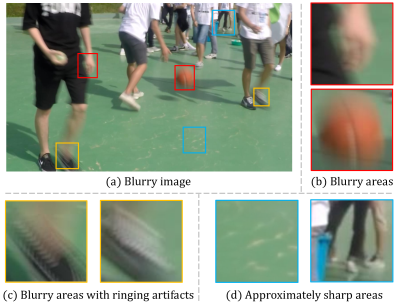
Figure 1: A blurry image example where the blur is non-uniform in (a). It includes some common blurry areas (b), severe blurry areas with ringing artifacts (c), and some approximately sharp areas (d).

Self-supervised denoising makes it possible to remove the noise without clean image supervision, but may give rise to obvious performance degradation, especially when handling complex real-world noises. Here we propose to alleviate this problem by introducing some extra supervision from the long-exposure counterpart. Obviously, taking the whole long-exposure image as supervision will bring adverse effects, making the results to be blurry. Nonetheless, it is worth noting that, the blur process $\mathcal{K}$ in Eqn. 1 is generally non-uniform, and sometimes not all areas are blurry. As shown in Fig. 1(d), there exist some approximately sharp regions in the long-exposure image, which can provide partial supervision information that benefits self-supervised denoising.

Therefore, it is crucial to pinpoint the sharp areas in the long-exposure image. Otherwise, we would prefer to go without sharp areas than accept a shoddy option, as misjudgments of sharp areas will lead to worse denoising results. However, without any discriminative clues, it is very likely to misjudge the sharp areas. Considering that $\mathbf{I}_{\mathcal{N}}$ is nearly non-blurry due to the short exposure time, it may be a reference for sharp area detection. To avoid noise interference, we pre-process $\mathbf{I}_{\mathcal{N}}$ with a self-supervised denoising model, and take the result $\mathbf{\tilde{I}}_{\mathcal{N}}$ to help detect sharp regions in the corresponding blurry image $\mathbf{I}_{\mathcal{B}}$.

Specifically, we first divide $\mathbf{I}_{\mathcal{B}}$ and $\mathbf{\tilde{I}}_{\mathcal{N}}$ into $\mathit{N}$ non-overlapping patches. For each patch pair $\mathbf{I}_{\mathcal{B}}^{\mathit{n}}$ and $\mathbf{\tilde{I}}_{\mathcal{N}}^{\mathit{n}}$ ($1\leq\mathit{n}\leq\mathit{N}$), our goal is to obtain a mask $\mathit{m}^{\mathit{n}}\in\{0,1\}$ that indicates whether $\mathbf{I}_{\mathcal{B}}^{\mathit{n}}$ is a sharp patch. Since $\mathbf{\tilde{I}}_{\mathcal{N}}$ is nearly non-blurry, when some severe motion blurs exist in $\mathbf{I}_{\mathcal{B}}^{\mathit{n}}$, the difference between $\mathbf{I}_{\mathcal{B}}^{\mathit{n}}$ and $\mathbf{\tilde{I}}_{\mathcal{N}}^{\mathit{n}}$ in textures and edges should be evident. Taking the above into account, we adopt a similarity metric $\mathit{s}$ to detect the areas with severe motion blurs, i.e.,

$$\mathit{m}^{\mathit{n}}=\mathtt{sgn}(\mathtt{max}(0,\mathit{s}(\mathbf{I}_{\mathcal{B}}^{\mathit{n}},\mathbf{\tilde{I}}_{\mathcal{N}}^{\mathit{n}})-\epsilon_{\mathit{s}})),$$ (7)

where structural similarity (SSIM) [41] is utilized for the similarity metric $\mathit{s}$, $\epsilon_{s}$ denotes the threshold, while $\mathtt{max}(a,b)$ and $\mathtt{sgn}(\cdot)$ denote the maximum and sign function, respectively.

However, the initial denoising result $\mathbf{\tilde{I}}_{\mathcal{N}}$ may be over-smooth, in other words, Eqn. 7 may fail when facing some mildly blurred regions in $\mathbf{I}_{\mathcal{B}}^{\mathit{n}}$. Therefore, we further measure the difference in variance between $\mathbf{I}_{\mathcal{B}}^{\mathit{n}}$ and $\mathbf{\tilde{I}}_{\mathcal{N}}^{\mathit{n}}$. When the variance of $\mathbf{I}_{\mathcal{B}}^{\mathit{n}}$ is greater than that of $\mathbf{\tilde{I}}_{\mathcal{N}}^{\mathit{n}}$, we consider that $\mathbf{I}_{\mathcal{B}}^{\mathit{n}}$ is potential to be a sharp patch. It should be noted that the difference in variance is not suitable for detecting some severely blurry areas with ringing artifacts (see Fig. 1(c)). In such blurry regions, the variance of $\mathbf{I}_{\mathcal{B}}^{\mathit{n}}$ may also be greater than that of $\mathbf{\tilde{I}}_{\mathcal{N}}^{\mathit{n}}$. When synthesizing blurry images, some works [24, 43, 57] remove the artifacts by interpolating the frames before averaging the sharp images. However, the artifacts also exist in real-world blurry images, especially in areas with flickering lights. Therefore, we still take the ringing artifacts into consideration in this work.

As a result, we jointly use the SSIM and variance measure for judging sharp regions, $\mathit{m}^{\mathit{n}}$ can be formulated as,

$$\mathit{m}^{\mathit{n}}=\mathtt{sgn}(\mathtt{max}(0,\mathit{s}(\mathbf{I}_{\mathcal{B}}^{\mathit{n}},\mathbf{\tilde{I}}_{\mathcal{N}}^{\mathit{n}})-\epsilon_{\mathit{s}}))*\mathtt{sgn}(\mathtt{max}(0,\mathtt{var}(\mathbf{I}_{\mathcal{B}}^{\mathit{n}})-\mathtt{var}(\mathbf{\tilde{I}}_{\mathcal{N}}^{\mathit{n}})-\epsilon_{\mathit{v}})),$$ (8)

where $\mathtt{var}(\cdot)$ and $\epsilon_{\mathit{v}}$ denote the variance function and the threshold, respectively. $\epsilon_{s}$ and $\epsilon_{v}$ are set to 0.99 and 1e-5 when color intensity values of $\mathbf{I}_{\mathcal{B}}^{\mathit{n}}$ and $\mathbf{\tilde{I}}_{\mathcal{N}}^{\mathit{n}}$ are normalized to $[0,1]$. Defining the final output image as $\mathbf{\hat{I}}$, the auxiliary loss function for denoising can be denoted as,

$$\mathcal{L}_{\mathit{aux}}(\mathbf{\hat{I}},\mathbf{I}_{\mathcal{B}})={\sum}_{\mathit{n}=1}^{\mathit{N}}\mathit{m}^{\mathit{n}}\|\mathbf{\hat{I}}^{\mathit{n}}-\mathbf{I}_{\mathcal{B}}^{\mathit{n}}\|_{2}^{2}.$$ (9)

3.3 Co-Learning of Deblurring and Denoising

\begin{overpic}[width=403.26341pt]{overview.pdf} \put(21.5,57.1){\scriptsize$\mathit{g}_{1}(\cdot)$} \put(23.3,46.8){\scriptsize$\mathit{g}_{1}(\cdot)$} \put(23.3,36.5){\scriptsize$\mathit{g}_{2}(\cdot)$} \put(35.3,20.6){\scriptsize$\mathit{g}_{1}(\cdot)$} \put(35.3,9.9){\scriptsize$\mathit{g}_{2}(\cdot)$} \par\put(14.3,47.8){\scriptsize($\mathbf{I}_{\mathcal{B}}$)} \put(14.0,31.8){\scriptsize($\mathbf{I}_{\mathcal{N}}$)} \par\put(30.0,50.9){\scriptsize$\mathit{g}_{1}(\mathbf{I}_{\mathcal{B}})$} \put(30.0,40.5){\scriptsize$\mathit{g}_{1}(\mathbf{I}_{\mathcal{N}})$} \put(30.0,30.2){\scriptsize$\mathit{g}_{2}(\mathbf{I}_{\mathcal{N}})$} \par\put(44.8,62.8){\scriptsize$\mathcal{L}_{\mathit{aux}}$} \put(44.2,60.8){\scriptsize\lx@cref{creftype~refnum}{loss:aux}} \put(42.4,35.8){\scriptsize$\mathcal{L}_{\mathit{rec}}\ \&\ \mathcal{L}_{\mathit{reg}}$} \put(40.8,33.6){\scriptsize\lx@cref{creftypeplural~refnum}{loss:rec} and~\lx@cref{refnum}{loss:reg}} \par\put(50.6,49.0){\scriptsize$\mathcal{D}$} \put(86.5,31.6){\scriptsize$\mathcal{D}$} \par\end{overpic}

Figure 2: Overview of our proposed SelfIR framework. (a) Training phase of SelfIR. Sub-sampled blurry image $\mathit{g}_{1}(\mathbf{I}_{\mathcal{B}})$ and noisy image $\mathit{g}_{1}(\mathbf{I}_{\mathcal{N}})$ are taken as the inputs. $\mathit{g}_{2}(\mathbf{I}_{\mathcal{N}})$ is used for calculating the reconstruction loss $\mathcal{L}_{\mathit{rec}}$ (see Eqn. 10) and regularization loss $\mathcal{L}_{\mathit{reg}}$ (see Eqn. 11), while $\mathit{g}_{1}(\mathbf{I}_{\mathcal{B}})$ is taken for calculating auxiliary loss (see Eqn. 9). (b) Example of neighbor sub-sampler. In each $2\times 2$ cell, two pixels are randomly selected for respectively composing the neighboring sub-images. (c) Testing phase of SelfIR. The blurry and noisy images can be directly taken for restoration.

As illustrated in Secs. 3.1 and 3.2, the noisy images can provide effective supervision information for deblurring, while the blurry images can also provide auxiliary supervision for self-supervised denoising. In other words, we can learn to deblur or denoise without additional clear and clean ground-truths. However, learning them independently will lead to limited performance. As some works [47, 23, 5, 14] have suggested, better restoration performance can be obtained by incorporating blurry with noisy images. Thus, it should be further considered to achieve self-supervised image restoration that takes two disturbed images as input. In this section, we delicately design the self-supervised model SelfIR that learns from both deblurring and denoising tasks in a collaborative learning manner.

For training SelfIR, it is required to avoid the trivial solution when taking both blurry and noisy images as the input. For example, when taking noisy images for supervising deblurring, the model may simply output the noisy images instead of learning the deburring results. Fortunately, Neighbor2Neighbor [11] shows the noises in two sub-sampled images (i.e., $\mathit{g}_{1}(\mathbf{I}_{\mathcal{N}})$ and $\mathit{g}_{2}(\mathbf{I}_{\mathcal{N}})$, see Fig. 2(b)) from noisy image $\mathbf{I}_{\mathcal{N}}$ are almost independent. Therefore, they can be respectively taken as the input and target for training the denoising subtask in a self-supervised manner. Simultaneously, combining the derivation in Eqn. 5, $\mathit{g}_{1}(\mathbf{I}_{\mathcal{B}})$ and $\mathit{g}_{2}(\mathbf{I}_{\mathcal{N}})$ can be respectively taken as the input and target to train the deblurring subtask. Therefore, our SelfIR can take a step forward and deliver both $\mathit{g}_{1}(\mathbf{I}_{\mathcal{B}})$ and $\mathit{g}_{1}(\mathbf{I}_{\mathcal{N}})$ ($i.e.$, $\{\mathit{g}_{1}(\mathbf{I}_{\mathcal{B}},\mathit{g}_{1}(\mathbf{I}_{\mathcal{N}})\}$) into the restoration network $\mathcal{D}$, as shown in Fig. 2(a). The sub-sampled image $\mathit{g}_{2}(\mathbf{I}_{\mathcal{N}})$ is taken for calculating reconstruction loss $\mathcal{L}_{\mathit{rec}}$, which can be written as,

$$\mathcal{L}_{\mathit{rec}}=\|\mathcal{D}(\mathit{g}_{1}(\mathbf{I}_{\mathcal{B}}),\mathit{g}_{1}(\mathbf{I}_{\mathcal{N}}))-\mathit{g}_{2}(\mathbf{I}_{\mathcal{N}})\|_{2}^{2}.$$ (10)

We also calculate regularization loss $\mathcal{L}_{\mathit{reg}}$ similar to [11],

$$\mathcal{L}_{\mathit{reg}}=\|\mathcal{D}(\mathit{g}_{1}(\mathbf{I}_{\mathcal{B}}),\mathit{g}_{1}(\mathbf{I}_{\mathcal{N}}))-\mathit{g}_{2}(\mathbf{I}_{\mathcal{N}})-(\mathit{g}_{1}(\hat{\mathcal{D}}(\mathbf{I}_{\mathcal{B}},\mathbf{I}_{\mathcal{N}}))-\mathit{g}_{2}(\hat{\mathcal{D}}(\mathbf{I}_{\mathcal{B}},\mathbf{I}_{\mathcal{N}})))\|_{2}^{2},$$ (11)

where $\hat{\mathcal{D}}$ has same parameters with $\mathcal{D}$ but has no gradient for back-propagation. Moreover, the sharp areas in $\mathit{g}_{1}(\mathbf{I}_{\mathcal{B}})$ can provide auxiliary supervision for the model learning and the performance can be further improved. Specifically, we calculate auxiliary loss $\mathcal{L}_{\mathit{aux}}(\mathcal{D}(\mathit{g}_{1}(\mathbf{I}_{\mathcal{B}}),\mathit{g}_{1}(\mathbf{I}_{\mathcal{N}}))),\mathit{g}_{1}(\mathbf{I}_{\mathcal{B}}))$ in Eqn. 9. For obtaining the mask $\mathit{m}^{\mathit{n}}$, we replace $\mathbf{I}_{\mathcal{B}}$ and $\mathbf{\tilde{I}}_{\mathcal{N}}$ in Eqn. 8 with $\mathit{g}_{1}(\mathbf{I}_{\mathcal{B}})$ and $\hat{\mathcal{D}}(\mathit{g}_{1}(\mathbf{I}_{\mathcal{B}}),\mathit{g}_{1}(\mathbf{I}_{\mathcal{N}}))$, respectively. Finally, the learning objective of parameters $\Theta_{\mathcal{D}}$ with the co-learning manner can be formulated as,

$$\Theta_{\mathcal{D}}^{\ast}=\operatorname*{\arg\min}_{\Theta_{\mathcal{D}}}\mathbb{E}_{\mathbf{I}_{\mathcal{B}},\mathbf{I}_{\mathcal{N}}}(\mathcal{L}_{\mathit{rec}}+\lambda_{\mathit{reg}}\mathcal{L}_{\mathit{reg}}+\lambda_{\mathit{aux}}\mathcal{L}_{\mathit{aux}}),$$ (12)

where $\lambda_{\mathit{reg}}$ and $\lambda_{\mathit{aux}}$ are hyper-parameters for balancing the loss terms.

4 Experiments

In this section, we first describe the dataset configuration and the training / evaluation protocols in detail. Then, both the quantitative and qualitative results on synthetic and real-world images are given for comprehensive evaluation.

4.1 Implementation Details

Synthetic Datasets. For synthesizing blurry images, early methods [47, 23] convolve sharp images with simulated blur kernels, which is quite different from the real-world blur model. Recently, the GoPro dataset [25] offers a more realistic way to synthesize blurry images, which has been widely adopted for motion deblurring tasks [25, 52, 39, 6, 51]. In the dataset, although slight inherent noise exists in the sharp video frames that are captured by a high-speed camera (i.e., GoPro Hero4 Black), it has little effect on model training and evaluation. We directly regard the sharp images as clean images. The blurry image is generated by averaging consecutive sharp frames, which can better simulate both camera shake and object motion. Thus, we can get the blurry-clear pairs as $\mathbf{I}_{\mathcal{B}}$ and $\mathbf{I}$, respectively. For synthesizing the noisy image $\mathbf{I}_{\mathcal{N}}$, we consider three noise distributions: 1) Gaussian noise with $\sigma\!\in\![5/255,50/255]$, 2) Poisson noise with $\lambda\!\in\![5,50]$, and 3) sensor noise [4]. Please refer to the supplementary material for the noise formulations. Experiments are conducted in both sRGB and raw-RGB spaces. For the sRGB space, we add Gaussian or Poisson noise to the sRGB sharp images. While for the raw-RGB space, the more complex sensor noise is added to the sharp raw-RGB images, and the blurry images are also converted back to the raw-RGB space through the unprocessing [4] pipeline. Finally, there are 2,103 image pairs for training, and we use the remaining 1,111 pairs for testing.

Real-world Datasets. Furthermore, we have also collected 61 real-world blurry and noisy raw-RGB pairs with Huawei P40 smartphones in the professional camera mode. In particular, the blurry images are captured with a low ISO and long exposure time, while the corresponding noisy images are captured with a high ISO and short exposure time in the same scene. Please refer to the supplementary material for detailed collection process. Due to the limited amount of real-world images, we use 30 pairs to fine-tune the model pre-trained on raw-RGB images with synthetic sensor noise, and take the remaining 31 pairs for evaluation.

Training Details. Following [17, 15, 11], we adopt a U-Net [33] architecture as our restoration network, where two encoders are respectively deployed to the blurry and noisy input images for better domain-specific feature extraction, and then blurry and noisy features are fused in the decoder part. Detailed architecture is given in the supplementary material. During training, the batch size is set to 16 and the patch size is $128\times 128$. Adam optimizer [12] with $\beta_{1}=0.9$ and $\beta_{2}=0.999$ is used to train the network for 200 epochs. The learning rate is initially set to $3\times 10^{-4}$ for synthetic experiments and $1\times 10^{-4}$ for real-world experiments. And it reduces by half every 50 epochs. For the hyper-parameters in Eqn. 12, $\lambda_{\mathit{aux}}$ is set to 2, $\lambda_{\mathit{reg}}$ is set to 2 and 4 for experiments in sRGB space and raw-RGB space, respectively. All experiments are conducted with PyTorch [28] on an Nvidia GeForce RTX 2080Ti GPU.

Evaluation Configurations. We convert all raw-RGB results to sRGB space through post-processing pipeline, and the quantitative metrics are computed in the sRGB space. For the results of synthetic experiments, we take peak signal to noise ratio (PSNR), structural similarity (SSIM) [41] and learned perceptual image patch similarity (LPIPS) [55] as evaluation metrics. For the results of real-world experiments, due to the lack of ground-truth images, we utilize no-reference IQA metrics (i.e., NIQE [22], NRQM [19], and PI [3]) to evaluate the generated images.

Table 1: Quantitative results on synthetic sRGB images.

	Method	Gaussian $\sigma\in[5/255,50/255]$ PSNR$\uparrow$ / SSIM$\uparrow$ / LPIPS$\downarrow$	Poisson $\lambda\in[5,50]$ PSNR$\uparrow$ / SSIM$\uparrow$ / LPIPS$\downarrow$
Supervised Deblurring	BaselineB	28.24 / 0.8561 / 0.191
	DeepDeblur [25]	30.04 / 0.9015 / 0.133
Supervised Denoising	BaselineN	34.91 / 0.9360 / 0.098	33.15 / 0.9225 / 0.126
	DnCNN [53]	34.63 / 0.9308 / 0.121	32.45 / 0.9084 / 0.128
Supervised IR	BaselineR	36.15 / 0.9534 / 0.070	34.74 / 0.9454 / 0.084
Self-Supervised Denoising	N2N [17]	34.88 / 0.9354 / 0.100	33.09 / 0.9216 / 0.129
	N2V [13]	33.09 / 0.9180 / 0.115	31.81 / 0.8999 / 0.137
	Laine19-mu [15]	33.61 / 0.9227 / 0.104	32.29 / 0.9091 / 0.131
	Laine19-pme [15]	34.76 / 0.9322 / 0.086	32.77 / 0.9147 / 0.116
	DBSN [44]	33.72 / 0.9224 / 0.111	31.46 / 0.8883 / 0.144
	R2R [27]	33.74 / 0.9223 / 0.100	30.05 / 0.7649 / 0.230
	Neighbor2Neighbor [11]	34.29 / 0.9271 / 0.085	32.68 / 0.9160 / 0.111
	Blind2Unblind [42]	34.69 / 0.9353 / 0.107	33.09 / 0.9216 / 0.132
Ours	SelfIR	35.74 / 0.9499 / 0.076	34.27 / 0.9404 / 0.092

4.2 Experimental Results in sRGB Space

To assess our proposed SelfIR, we build several baseline methods for comparison, including 1) a supervised deblurring baseline (denoted by Baseline_B), 2) a supervised denoising baseline (denoted by Baseline_N), 3) a supervised image restoration baseline which takes both blurry and noisy images as input (denoted by Baseline_R), and 4) Neighbor2Neighbor [11] since the denoising part of our co-learning framework is based on it. Note that the network structure is not the focus of this paper, so we deploy a simple U-Net [33] architecture for our restoration network $\mathcal{D}$ and the first three baseline methods. Besides, we choose two classical supervised methods (i.e., DeepDeblur [25] and DnCNN [53]) for comparison. Self-supervised denoising methods (e.g., N2N [17], N2V [13], Laine19 [15], DBSN [44], R2R [27], and Blind2Unblind [42]) are also compared. For DeepDeblur [25], we use the officially released model for testing. For other methods, the models are retrained with our synthetic images for a fair comparison.

The quantitative results of synthetic experiments on Gaussian and Poisson noise are given in Tab. 1. One can see that our SelfIR outperforms all other methods except the supervised IR model (Baseline_R), which can be seen as the upper limit of the restoration performance with the utilized U-Net architecture and the blurry-noisy pair input. In comparison to the self-supervised denoising baseline Neighbor2Neighbor [11], 1.45 dB and 1.59 dB PSNR gains are obtained by our SelfIR on Gaussian and Poisson noise, respectively. Even compared to the supervised denoising baseline model (Baseline_N), our method also improves the PSNR index by 0.83 dB and 1.12 dB. Due to the severely ill-posed nature of deblurring, SelfIR brings a PSNR gain by more than 6 dB comparing to the supervised deblurring baseline model (Baseline_B). The results clearly show that the blurry images can indeed provide beneficial features for denoising, and so do the noisy images for deblurring.

The qualitative results are shown in Figs. 7 and 9. One can see that our results are sharper and clearer than other denoising or deblurring methods. In terms of visual quality, the proposed SelfIR is almost comparable to the supervised image restoration model (Baseline_R), and combines the advantages of supervised denoising Baseline_N and deblurring Baseline_B. More results can be found in the supplemental material.

(a) Noisy Image

(b) Baseline_N

(c) N2V [13]

(d) Laine19-pme [15]

(e) DBSN [44]

(f) R2R [27]

(g) Blurry Image

(h) Baseline_B

(i) Neighbor2Neighbor [11]

(j) Blind2Unblind [42]

(k) SelfIR (Ours)

(l) Baseline_R

Figure 3: Visual comparison on Gaussian noise. The texts in our result are sharper and clearer. The proposed SelfIR is almost comparable to supervised Baseline_R, which can be seen as the upper limit of the restoration performance with the utilized U-Net architecture and the blurry-noisy pair input.

(a) Noisy Image

(b) Baseline_N

(c) N2V [13]

(d) Laine19-pme [15]

(e) DBSN [44]

(f) R2R [27]

(g) Blurry Image

(h) Baseline_B

(i) Neighbor2Neighbor [11]

(j) Blind2Unblind [42]

(k) SelfIR (Ours)

(l) Baseline_R

Figure 4: Visual comparison on Poisson noise. In terms of the visual result, SelfIR combines the advantages of supervised denoising Baseline_N and deblurring Baseline_B.

Table 2: Quantitative results on synthetic and real-world raw-RGB images.

	Method	Sensor Noise [4] PSNR$\uparrow$ / SSIM$\uparrow$ / LPIPS$\downarrow$	Real-World Images NIQE$\downarrow$ / NRQM$\uparrow$ / PI$\downarrow$
Supervised Deblurring	BaselineB	28.14 / 0.8547 / 0.162	6.26 / 5.04 / 5.62
	DeepDeblur [25]	29.75 / 0.8881 / 0.115	6.76 / 4.78 / 6.00
Supervised Denoising	BaselineN	34.52 / 0.9461 / 0.053	5.69 / 4.85 / 5.43
	DnCNN [53]	33.81 / 0.9325 / 0.076	6.05 / 5.10 / 5.48
Supervised IR	BaselineR	36.10 / 0.9574 / 0.035	5.54 / 5.14 / 5.18
Self-Supervised Denoising	N2N [17]	34.67 / 0.9472 / 0.053	6.10 / 4.93 / 5.59
	N2V [13]	31.39 / 0.9227 / 0.076	5.82 / 5.52 / 5.17
	Laine19-mu [15]	32.74 / 0.9304 / 0.073	5.87 / 5.67 / 5.10
	Laine19-pme [15]	33.28 / 0.9119 / 0.095	7.26 / 6.03 / 5.62
	DBSN [44]	33.59 / 0.9389 / 0.060	6.57 / 5.48 / 5.54
	R2R [27]	32.21 / 0.8807 / 0.117	5.63 / 5.63 / 4.99
	Neighbor2Neighbor [11]	32.82 / 0.9275 / 0.087	6.47 / 5.86 / 5.33
	Blind2Unblind [42]	33.30 / 0.9380 / 0.061	5.28 / 5.22 / 5.04
Ours	SelfIR	34.51 / 0.9440 / 0.053	5.48 / 5.83 / 4.86

4.3 Experimental Results in Raw-RGB Space

Tab. 2 shows the quantitative results of synthetic and real-world experiments on raw-RGB images. For synthetic experiments with more complex and realistic sensor noise [4], all models are retrained with our synthetic images. Our SelfIR achieves a 1.69 dB PSNR gain in comparison with Neighbor2Neighbor [11]. For evaluation on real-world images, we directly use the models of N2N [17], Laine19-pme [15], R2R [27] and all supervised methods, which are pre-trained for sensor noise. For SelfIR and other self-supervised methods, we fine-tune the pre-trained model on our real-world training set. The PI [3] metric of SelfIR is improved by 0.55 on real-world testing images through fine-tuning. And the results on no-reference IQA show that our method is very competitive in comparison with the competing methods on real-world images. The visual results are given in the supplemental material.

Table 3: Results of deblurring with clear images and noisy images as the supervision.

Supervision Information	Gaussian $\sigma\in[5/255,50/255]$ PSNR$\uparrow$ / SSIM$\uparrow$ / LPIPS$\downarrow$	Poisson $\lambda\in[5,50]$ PSNR$\uparrow$ / SSIM$\uparrow$ / LPIPS$\downarrow$	Sensor Noise [4] PSNR$\uparrow$ / SSIM$\uparrow$ / LPIPS$\downarrow$
Clear Images	28.24 / 0.8561 / 0.191	28.24 / 0.8561 / 0.191	28.14 / 0.8547 / 0.162
Noisy Images	28.29 / 0.8578 / 0.190	28.23 / 0.8563 / 0.191	28.16 / 0.8545 / 0.164

Table 4: Ablation study of auxiliary loss on Gaussian noise.

	Neighbor2Neighbor [11] PSNR$\uparrow$ / SSIM$\uparrow$ / LPIPS$\downarrow$	SelfIR PSNR$\uparrow$ / SSIM$\uparrow$ / LPIPS$\downarrow$
w/o $\mathcal{L}_{aux}$	34.29 / 0.9271 / 0.085	35.65 / 0.9492 / 0.080
w/ $\mathcal{L}_{aux}$	34.45 / 0.9307 / 0.093	35.74 / 0.9499 / 0.076

5 Ablation Study

5.1 Feasibility of Deblurring with Noisy Images

In order to verify the feasibility of taking noisy images as the supervision of deblurring in Sec. 3.1, we replace the clear supervision of Baseline_B with noisy images of different noise distributions, and the results are shown in Tab. 3. It can be seen that taking noisy or clear images as the supervision leads to similar performance on the deblurring task, which confirms that the noisy images can be an alternative of clear images to supervise the deblurring task.

5.2 Effect of Auxiliary Loss

In order to evaluate the effect of auxiliary loss $\mathcal{L}_{aux}$ in Eqn. 9, we add $\mathcal{L}_{aux}$ to the loss terms of self-supervised denoising method Neighbor2Neighbor [11]. As shown in Tab. 4, we obtain 0.16 dB PSNR gain against the baseline Neighbor2Neighbor [11]. The result indicates that blurry images can provide some auxiliary supervision information and improve performance for self-supervised denoising. When removing $\mathcal{L}_{aux}$ from our SelfIR, the PSNR dropped by 0.09 dB. Since the long-exposure image is taken directly as input, the loss term may be less effective, but is still beneficial.

Table 5: Ablation study on different weights ($\lambda_{reg}$ values) of regularization loss.

$\lambda_{reg}$	PSNR$\uparrow$ / SSIM$\uparrow$ / LPIPS$\downarrow$
0	35.20 / 0.9473 / 0.097
1	35.64 / 0.9492 / 0.082
2	35.74 / 0.9499 / 0.076
4	35.72 / 0.9496 / 0.075
8	35.73 / 0.9497 / 0.072

Table 6: Ablation study on different weights ($\lambda_{aux}$ values) of auxiliary loss.

$\lambda_{aux}$	PSNR$\uparrow$ / SSIM$\uparrow$ / LPIPS$\downarrow$
0	35.65 / 0.9492 / 0.080
1	35.73 / 0.9498 / 0.078
2	35.74 / 0.9499 / 0.076
4	35.73 / 0.9499 / 0.076
8	35.67 / 0.9496 / 0.077

5.3 Effect of Different Loss Weights

We conduct ablation studies on different weighting hyper-parameters (i.e., $\lambda_{reg}$ and $\lambda_{reg}$) for balancing regularization and auxiliary loss terms. The experiments are conducted on Gaussian noise in sRGB space. When varying one hyper-parameter, the other one is set to 2 by default. As shown in Tabs. 5 and  6, it can be seen that the sensitivity to $\lambda_{reg}$ and $\lambda_{reg}$ of SelfIR is acceptable.

6 Conclusion

The complementarity between long-exposure blurry and short-exposure noisy images not only improves the performance of image restoration, but also makes it possible to learn a restoration model in a self-supervised manner. Jointly leveraging the long- and short-exposure images, we present a self-supervised image restoration method named SelfIR. On the one hand, we take the short-exposure images as the supervision information for deblurring. On the other hand, we utilize the sharp areas in the long-exposure images as auxiliary supervision information in aid of self-supervised denoising. SelfIR combines these two aspects by a collaborative learning scheme, and makes the deblurring and denoising tasks benefit from each other. Experiments on synthetic and real-world images show the effectiveness and practicality of our proposed method.

7 Limitation, Impact, Etc

This work is still limited in assessing the results on real-world image pairs. Although no-reference IQA metrics are adopted, these may be too unstable to report the performance consistent with humans accurately. We will establish a real-world blurry-noisy pair dataset including high-quality GTs to solve this problem in the future work. As for societal influence, this work is promising to be applied to terminal devices (e.g., smartphones) for obtaining better images under low-light environments. It has no foreseeable negative impact. Besides, the images used in this work are from natural or human scenes. The GoPro dataset used for synthetic experiments is public under CC BY 4.0 license. There is no personally identifiable information or offensive content in the experimental data.

Appendix

Appendix A Content

The content of the supplementary material involves:

• Formulations of synthetic noise in Sec. B.

• Detailed collection process of real-world dataset in Sec. C.

• Detailed architecture of restoration network in Sec. D.

• More qualitative results in Sec. E.

Appendix B Formulations of Synthetic Noise

Gaussian Noise. Sensor noise mainly includes shot and read noise, which are caused by photon arrival statistics biases and imprecise readout circuits, respectively. Gaussian noise is a good approximation of read noise and is widely used as the assumption for denoising. In the experiments, the synthetic Gaussian noise $\mathbf{N}_{\mathcal{N}}$ for the short-exposure image can be expressed as,

$$\mathbf{N}_{\mathcal{N}}\sim\mathcal{N}(\mathbf{0},\sigma^{2}\mathbf{E})$$ (13)

where $\mathcal{N}(\cdot,\cdot)$ denotes Gaussian distribution, $\mathbf{E}$ is an identity matrix with ones on the main diagonal and zeros elsewhere. Following previous works [11, 42], the standard deviation $\sigma$ is chosen uniformly at random from $[5/255,50/255]$ when color intensity values of images are normalized to $[0,1]$.

Poisson Noise. During imaging, the sensor receives photons and performs the photoelectric conversion. The quantum nature of light leads to uncertainty in the number of electrons, which introduces shot noise in the image. The shot noise follows a Poisson distribution $\mathcal{P}$ over the number of electrons, thus we also experiment using the noisy image $\mathbf{I}_{\mathcal{N}}$ with Poisson noise, which can be expressed as,

$$\mathbf{I}_{\mathcal{N}}\sim\mathcal{P}(\lambda\cdot\mathbf{I})/\lambda,$$ (14)

where $\mathbf{I}$ denotes a clean image, $\lambda\!\in\![5,50]$ according to  [11, 42].

Sensor Noise. Recently, Brook et al. [4] propose to approximate shot and read noise as a single heteroscedastic Gaussian noise. The noise is more complex but more realistic than homoscedastic Gaussian or Poisson noise, which can be written as,

$$\mathbf{N}_{\mathcal{N}}\sim\mathcal{N}(\mathbf{0},\lambda_{read}+\lambda_{shot}\mathbf{I}).$$ (15)

where $\lambda_{read}$ and $\lambda_{shot}$ are determined by modeling the joint distribution of different shot/read noise parameter pairs in real-world raw images and sampling from that distribution. For SIDD [1] dataset, the sampling shot/read noise factors can be expressed as,

$$\begin{split}&\log(\lambda_{shot})\sim{\mathcal{U}}(\log(0.00068674),\log(0.02194856)),\\ &\log(\lambda_{read})\mid\log(\lambda_{shot})\sim{\mathcal{N}}(1.85\lambda_{shot}+0.3,0.2^{2}).\end{split}$$ (16)

where $\mathcal{U}(a,b)$ denotes a uniform distribution in the range $[a,b]$.

Appendix C Detailed Collection Process of Real-World Dataset

For obtaining real-world blurry-noisy image pairs, we utilize two Huawei P40 smartphones to capture a short-exposure noisy image and a long-exposure blurry image of the same scene, respectively. In the pair, the product of ISO and exposure time of two images remains the same, i.e., the noisy image is captured with a high ISO and short exposure time, while the blurry one is captured with a low ISO and long exposure time. In order to make the captured image pair align as much as possible, the two smartphones take images side by side at the same time. Nonetheless, spatial misalignment still exists between the image pair, as the two camera lenses are not in the same position.

Therefore, we further exploit the optical flow network PWC-Net [38] to align the image pair. First, the raw-RGB pair is converted to sRGB space through camera image signal processing (ISP) pipeline. Then we calculate the optical flow between the sRGB image pair and use the optical flow to warp raw-RGB blurry image. Finally, the approximately aligned blurry-noisy raw-RGB pair can be obtained. Fig. 5 shows two examples of our real-world blurry-noisy image pairs.

(a)

(b)

(c) Short-Exposure Noisy Image

(d) Long-Exposure Blurry Image

Figure 5: Example image patches of our real-world blurry-noisy pairs.

Appendix D Detailed Architecture of Restoration Network

Fig. 6 shows the detailed architecture of restoration network. Two encoders are respectively deployed to the blurry and noisy input images for better domain-specific feature extraction, and then blurry and noisy features are fused in the decoder part. The architectures of encoder and decoder are the same with these of previous self-supervised denoising methods [17, 15, 11].

\begin{overpic}[width=429.28616pt]{network2.pdf} \end{overpic}

Figure 6: Architecture of restoration network. $E_{i}^{B}$ and $E_{i}^{N}$ denote the $i$-th level of encoder for noisy image and blurry image, respectively. $D_{i}$ denotes the $i$-th level of decoder.

Appendix E More Qualitative Results

Figs. 7 and 8 show more qualitative results on Gaussian noise. Figs. 9 and 10 show more qualitative results on Poisson noise. The visual comparison on sensor noise [4] can be seen in Figs. 11 and 12. The visual comparison on the real-world images can be seen in Figs. 13 and 14. The results show our SelfIR performs favorably against the state-of-the-art self-supervised denoising methods, as well as the baseline supervised deblurring and denoising methods.

(a) Noisy Image

(b) Baseline_N

(c) N2V [13]

(d) Laine19-pme [15]

(e) DBSN [44]

(f) R2R [27]

(g) Blurry Image

(h) Baseline_B

(i) Neighbor2Neighbor [11]

(j) Blind2Unblind [42]

(k) SelfIR (Ours)

(l) GT

Figure 7: Visual comparison on Gaussian noise. The lines and chair in our result are clearer.

(a) Noisy Image

(b) Baseline_N

(c) N2V [13]

(d) Laine19-pme [15]

(e) DBSN [44]

(f) R2R [27]

(g) Blurry Image

(h) Baseline_B

(i) Neighbor2Neighbor [11]

(j) Blind2Unblind [42]

(k) SelfIR (Ours)

(l) GT

Figure 8: Visual comparison on Gaussian noise. The edges of tree and steps in our result are sharper.

(a) Noisy Image

(b) Baseline_N

(c) N2V [13]

(d) Laine19-pme [15]

(e) DBSN [44]

(f) R2R [27]

(g) Blurry Image

(h) Baseline_B

(i) Neighbor2Neighbor [11]

(j) Blind2Unblind [42]

(k) SelfIR (Ours)

(l) GT

Figure 9: Visual comparison on Poisson noise. Our SelfIR recovers more fine-scale textures.

(a) Noisy Image

(b) Baseline_N

(c) N2V [13]

(d) Laine19-pme [15]

(e) DBSN [44]

(f) R2R [27]

(g) Blurry Image

(h) Baseline_B

(i) Neighbor2Neighbor [11]

(j) Blind2Unblind [42]

(k) SelfIR (Ours)

(l) GT

Figure 10: Visual comparison on Poisson noise. The textures in our result are clearer and more regular.

(a) Noisy Image

(b) Baseline_N

(c) N2V [13]

(d) Laine19-pme [15]

(e) DBSN [44]

(f) R2R [27]

(g) Blurry Image

(h) Baseline_B

(i) Neighbor2Neighbor [11]

(j) Blind2Unblind [42]

(k) SelfIR (Ours)

(l) GT

Figure 11: Visual comparison on sensor noise. Our result is more photo-realistic and faithfully recovers the image color.

(a) Noisy Image

(b) Baseline_N

(c) N2V [13]

(d) Laine19-pme [15]

(e) DBSN [44]

(f) R2R [27]

(g) Blurry Image

(h) Baseline_B

(i) Neighbor2Neighbor [11]

(j) Blind2Unblind [42]

(k) SelfIR (Ours)

(l) GT

Figure 12: Visual comparison on sensor noise. Our SelfIR recovers much more details.

(a) Noisy Image

(b) Baseline_N

(c) N2V [13]

(d) Laine19-pme [15]

(e) DBSN [44]

(f) R2R [27]

(g) Blurry Image

(h) Baseline_B

(i) Neighbor2Neighbor [11]

(j) Blind2Unblind [42]

(k) SelfIR (Ours)

(l) Baseline_R

Figure 13: Visual comparison on real-world images. Our result is clearer and more photo-realistic.

(a) Noisy Image

(b) Baseline_N

(c) N2V [13]

(d) Laine19-pme [15]

(e) DBSN [44]

(f) R2R [27]

(g) Blurry Image

(h) Baseline_B

(i) Neighbor2Neighbor [11]

(j) Blind2Unblind [42]

(k) SelfIR (Ours)

(l) Baseline_R

Figure 14: Visual comparison on real-world images. The license plate in our result is clearer and sharper.

References

- [1] Abdelrahman Abdelhamed, Stephen Lin, and Michael S Brown. A high-quality denoising dataset for smartphone cameras. In CVPR, 2018.
- [2] Miika Aittala and Frédo Durand. Burst image deblurring using permutation invariant convolutional neural networks. In ECCV, 2018.
- [3] Yochai Blau, Roey Mechrez, Radu Timofte, Tomer Michaeli, and Lihi Zelnik-Manor. The 2018 pirm challenge on perceptual image super-resolution. In ECCV Workshops, 2018.
- [4] Tim Brooks, Ben Mildenhall, Tianfan Xue, Jiawen Chen, Dillon Sharlet, and Jonathan T Barron. Unprocessing images for learned raw denoising. In CVPR, 2019.
- [5] Meng Chang, Huajun Feng, Zhihai Xu, and Qi Li. Low-light image restoration with short-and long-exposure raw pairs. IEEE TMM, 2021.
- [6] Sung-Jin Cho, Seo-Won Ji, Jun-Pyo Hong, Seung-Won Jung, and Sung-Jea Ko. Rethinking coarse-to-fine approach in single image deblurring. In ICCV, 2021.
- [7] Mauricio Delbracio, Damien Kelly, Michael S Brown, and Peyman Milanfar. Mobile computational photography: A tour. Annual Review of Vision Science, 2021.
- [8] Rob Fergus, Barun Singh, Aaron Hertzmann, Sam T Roweis, and William T Freeman. Removing camera shake from a single photograph. In ACM SIGGRAPH, 2006.
- [9] Shi Guo, Zifei Yan, Kai Zhang, Wangmeng Zuo, and Lei Zhang. Toward convolutional blind denoising of real photographs. In CVPR, 2019.
- [10] Samuel W Hasinoff, Dillon Sharlet, Ryan Geiss, Andrew Adams, Jonathan T Barron, Florian Kainz, Jiawen Chen, and Marc Levoy. Burst photography for high dynamic range and low-light imaging on mobile cameras. ACM ToG, 2016.
- [11] Tao Huang, Songjiang Li, Xu Jia, Huchuan Lu, and Jianzhuang Liu. Neighbor2neighbor: Self-supervised denoising from single noisy images. In CVPR, 2021.
- [12] Diederik P Kingma and Jimmy Ba. Adam: A method for stochastic optimization. In ICLR, 2015.
- [13] Alexander Krull, Tim-Oliver Buchholz, and Florian Jug. Noise2void-learning denoising from single noisy images. In CVPR, 2019.
- [14] Green Rosh KS, Nikhil Krishnan, BH Pawan Prasad, and Sachin Lomte. Content preserving scale space network for fast image restoration from noisy-blurry pairs. In ICASSP, 2022.
- [15] Samuli Laine, Tero Karras, Jaakko Lehtinen, and Timo Aila. High-quality self-supervised deep image denoising. In NeurIPS, 2019.
- [16] Wooseok Lee, Sanghyun Son, and Kyoung Mu Lee. Ap-bsn: Self-supervised denoising for real-world images via asymmetric pd and blind-spot network. In CVPR, 2022.
- [17] Jaakko Lehtinen, Jacob Munkberg, Jon Hasselgren, Samuli Laine, Tero Karras, Miika Aittala, and Timo Aila. Noise2noise: Learning image restoration without clean data. In ICML, 2018.
- [18] Pengju Liu, Hongzhi Zhang, Kai Zhang, Liang Lin, and Wangmeng Zuo. Multi-level wavelet-cnn for image restoration. In CVPR, 2018.
- [19] Chao Ma, Chih-Yuan Yang, Xiaokang Yang, and Ming-Hsuan Yang. Learning a no-reference quality metric for single-image super-resolution. Computer Vision and Image Understanding, 2017.
- [20] Tomer Michaeli and Michal Irani. Blind deblurring using internal patch recurrence. In ECCV, 2014.
- [21] Ben Mildenhall, Jonathan T Barron, Jiawen Chen, Dillon Sharlet, Ren Ng, and Robert Carroll. Burst denoising with kernel prediction networks. In CVPR, 2018.
- [22] Anish Mittal, Rajiv Soundararajan, and Alan C Bovik. Making a “completely blind” image quality analyzer. IEEE Signal Processing Letters, 2012.
- [23] Janne Mustaniemi, Juho Kannala, Jiri Matas, Simo Särkkä, and Janne Heikkilä. Lsd2–joint denoising and deblurring of short and long exposure images with cnns. In BMVC, 2020.
- [24] Seungjun Nah, Sungyong Baik, Seokil Hong, Gyeongsik Moon, Sanghyun Son, Radu Timofte, and Kyoung Mu Lee. Ntire 2019 challenge on video deblurring and super-resolution: Dataset and study. In CVPR Workshops, 2019.
- [25] Seungjun Nah, Tae Hyun Kim, and Kyoung Mu Lee. Deep multi-scale convolutional neural network for dynamic scene deblurring. In CVPR, 2017.
- [26] Reyhaneh Neshatavar, Mohsen Yavartanoo, Sanghyun Son, and Kyoung Mu Lee. Cvf-sid: Cyclic multi-variate function for self-supervised image denoising by disentangling noise from image. In CVPR, 2022.
- [27] Tongyao Pang, Huan Zheng, Yuhui Quan, and Hui Ji. Recorrupted-to-recorrupted: Unsupervised deep learning for image denoising. In CVPR, 2021.
- [28] Adam Paszke, Sam Gross, Francisco Massa, Adam Lerer, James Bradbury, Gregory Chanan, Trevor Killeen, Zeming Lin, Natalia Gimelshein, Luca Antiga, Alban Desmaison, Andreas Kopf, Edward Yang, Zachary DeVito, Martin Raison, Alykhan Tejani, Sasank Chilamkurthy, Benoit Steiner, Lu Fang, Junjie Bai, and Soumith Chintala. Pytorch: An imperative style, high-performance deep learning library. In NeurIPS, 2019.
- [29] Tobias Plotz and Stefan Roth. Benchmarking denoising algorithms with real photographs. In CVPR, 2017.
- [30] Dongwei Ren, Kai Zhang, Qilong Wang, Qinghua Hu, and Wangmeng Zuo. Neural blind deconvolution using deep priors. In CVPR, 2020.
- [31] Wenqi Ren, Jiawei Zhang, Lin Ma, Jinshan Pan, Xiaochun Cao, Wangmeng Zuo, Wei Liu, and Ming-Hsuan Yang. Deep non-blind deconvolution via generalized low-rank approximation. In NeurIPS, 2018.
- [32] Jaesung Rim, Haeyun Lee, Jucheol Won, and Sunghyun Cho. Real-world blur dataset for learning and benchmarking deblurring algorithms. In ECCV, 2020.
- [33] Olaf Ronneberger, Philipp Fischer, and Thomas Brox. U-net: Convolutional networks for biomedical image segmentation. In MICCAI, 2015.
- [34] Christian J Schuler, Michael Hirsch, Stefan Harmeling, and Bernhard Schölkopf. Learning to deblur. IEEE TPAMI, 2015.
- [35] Qi Shan, Jiaya Jia, and Aseem Agarwala. High-quality motion deblurring from a single image. ACM TOG, 2008.
- [36] Ziyi Shen, Wenguan Wang, Xiankai Lu, Jianbing Shen, Haibin Ling, Tingfa Xu, and Ling Shao. Human-aware motion deblurring. In ICCV, 2019.
- [37] Shakarim Soltanayev and Se Young Chun. Training deep learning based denoisers without ground truth data. In NeurIPS, 2018.
- [38] Deqing Sun, Xiaodong Yang, Ming-Yu Liu, and Jan Kautz. Pwc-net: Cnns for optical flow using pyramid, warping, and cost volume. In CVPR, 2018.
- [39] Xin Tao, Hongyun Gao, Xiaoyong Shen, Jue Wang, and Jiaya Jia. Scale-recurrent network for deep image deblurring. In CVPR, 2018.
- [40] Dmitry Ulyanov, Andrea Vedaldi, and Victor Lempitsky. Deep image prior. In CVPR, 2018.
- [41] Zhou Wang, Alan C Bovik, Hamid R Sheikh, and Eero P Simoncelli. Image quality assessment: from error visibility to structural similarity. IEEE TIP, 2004.
- [42] Zejin Wang, Jiazheng Liu, Guoqing Li, and Hua Han. Blind2unblind: Self-supervised image denoising with visible blind spots. In CVPR, 2022.
- [43] Patrick Wieschollek, Michael Hirsch, Bernhard Scholkopf, and Hendrik Lensch. Learning blind motion deblurring. In ICCV, 2017.
- [44] Xiaohe Wu, Ming Liu, Yue Cao, Dongwei Ren, and Wangmeng Zuo. Unpaired learning of deep image denoising. In ECCV, 2020.
- [45] Zhihao Xia, Federico Perazzi, Michaël Gharbi, Kalyan Sunkavalli, and Ayan Chakrabarti. Basis prediction networks for effective burst denoising with large kernels. In CVPR, 2020.
- [46] Li Xu, Shicheng Zheng, and Jiaya Jia. Unnatural l0 sparse representation for natural image deblurring. In CVPR, 2013.
- [47] Lu Yuan, Jian Sun, Long Quan, and Heung-Yeung Shum. Image deblurring with blurred/noisy image pairs. In SIGGRAPH, 2007.
- [48] Zongsheng Yue, Qian Zhao, Lei Zhang, and Deyu Meng. Dual adversarial network: Toward real-world noise removal and noise generation. In ECCV, 2020.
- [49] Syed Waqas Zamir, Aditya Arora, Salman Khan, Munawar Hayat, Fahad Shahbaz Khan, and Ming-Hsuan Yang. Restormer: Efficient transformer for high-resolution image restoration. In CVPR, 2022.
- [50] Syed Waqas Zamir, Aditya Arora, Salman Khan, Munawar Hayat, Fahad Shahbaz Khan, Ming-Hsuan Yang, and Ling Shao. Learning enriched features for real image restoration and enhancement. In ECCV, 2020.
- [51] Syed Waqas Zamir, Aditya Arora, Salman Khan, Munawar Hayat, Fahad Shahbaz Khan, Ming-Hsuan Yang, and Ling Shao. Multi-stage progressive image restoration. In CVPR, 2021.
- [52] Jiawei Zhang, Jinshan Pan, Jimmy Ren, Yibing Song, Linchao Bao, Rynson WH Lau, and Ming-Hsuan Yang. Dynamic scene deblurring using spatially variant recurrent neural networks. In CVPR, 2018.
- [53] Kai Zhang, Wangmeng Zuo, Yunjin Chen, Deyu Meng, and Lei Zhang. Beyond a gaussian denoiser: Residual learning of deep cnn for image denoising. IEEE TIP, 2017.
- [54] Kai Zhang, Wangmeng Zuo, and Lei Zhang. Ffdnet: Toward a fast and flexible solution for cnn-based image denoising. IEEE TIP, 2018.
- [55] Richard Zhang, Phillip Isola, Alexei A Efros, Eli Shechtman, and Oliver Wang. The unreasonable effectiveness of deep features as a perceptual metric. In CVPR, 2018.
- [56] Yi Zhang, Dasong Li, Ka Lung Law, Xiaogang Wang, Hongwei Qin, and Hongsheng Li. Idr: Self-supervised image denoising via iterative data refinement. In CVPR, 2022.
- [57] Shangchen Zhou, Jiawei Zhang, Wangmeng Zuo, Haozhe Xie, Jinshan Pan, and Jimmy S Ren. Davanet: Stereo deblurring with view aggregation. In CVPR, 2019.
- [58] Magauiya Zhussip, Shakarim Soltanayev, and Se Young Chun. Extending stein’s unbiased risk estimator to train deep denoisers with correlated pairs of noisy images. In NeurIPS, 2019.