Bayesian Layer Graph Convolutional Network for Hyperspectral Image Classification

Abstract

In recent years, research on hyperspectral image (HSI) classification has continuous progress on introducing deep network models, and recently the graph convolutional network (GCN) based models have shown impressive performance. However, these deep learning frameworks are based on point estimation suffering from low generalization and inability to quantify the classification results uncertainty. On the other hand, simply applying the distribution estimation based Bayesian Neural Network (BNN) to classify the HSI is unable to achieve high classification efficiency due to the large amount of parameters. In this paper, we design a Bayesian layer as an insertion layer into point estimation based neural networks, and propose a Bayesian layer graph convolutional network (BLGCN) model by combining graph convolution operations, which can effectively extract graph information and estimate the uncertainty of classification results. Moreover, a Generative Adversarial Network (GAN) is built to solve the sample imbalance problem of HSI dataset. Finally, we design a dynamic control training strategy based on the confidence interval of the classification results, which will terminate the training early when the confidence interval reaches the presented threshold. The experimental results show that our model achieves a balance between high classification accuracy and strong generalization. In addition, it can quantify the uncertainty of outputs.

I Introduction

With the rapid development of remote sensing sensors, hyperspectral images have drawn more and more attentions in academic research and various applications [1, 2], such as mineral detection, soil testing, medical image, and urban planning. Compared with conventional optical remote sensing image, hyperspectral images contain abundant spectral information, which are consists of hundreds of contiguous spectral channels [3, 4]. Due to this character, besides spatial context information, hyperspectral images possess unique spectral signatures for identifying materials and ground truth. For the last few years, spatial-spectral classification for hyperspectral images has become a hot research issue in remote sensing society.

In early researches, hyperspectral image classification focuses on designing various feature extraction methods manually. Feature extraction is designed to mapping the original data into a new feature space where the spatial and spectral features are more distinguished and better for classification. For spectral feature extraction, there are two main methods: linear transformation based methods and nonlinear transformation based methods. Principal component analysis (PCA) [5] and independent component analysis (ICA) [6] are two representative methods for linear transformation based methods. They use matrix factorization to obtain a new feature space. For nonlinear transformation based methods, locally linear embedding (LLE) [7] and locality preserving projections (LPP) [8] based methods are two conventional feature extraction methods in pattern recognition, which are based on manifold learning for seeking new feature space. However, researchers found that only extracting spectral features has limited improvement in classification accuracy. Since spatially adjacent ground truth is more relevant [9], spatial context features are also considered for feature extraction combined with spectral features. Random field based methods are classic spatial feature extraction methods. Thereinto, Markov random field (MRF) and conditional random field (CRF) are two representative ones. MRF can build models according to the relevance of adjacent pixels, which can be used in multiple ground truth scenes and multiple distribution models. Many works have been proposed based on MRF. For example, an adaptive MRF was proposed for hyperspectral feature extraction [10]. Further, Sun proposed a spatially adaptive Markov random field (MRF) prior in the hidden field [11], which makes the spatial term more smooth. CRF is a probabilistic model for labels and structural data, which shows potentials for spatial feature extraction. Various CRF-based methods have been proposed for spatial feature extraction, such as CRF combined with sparse representation [12], CRF combined with ensemble learning [13], and CRF combined with sub-pixel techniques [14]. Besides, morphological feature based methods are also effective ways for spatial feature extraction, among which, extended morphological attribute profiles (EMAP) is a representative one [15]. Based on EMAP, some solid works have been proposed, such as multiple feature learning [16] and histogram-based attribute profiles methods [17].

The conventional manually designed feature extraction methods consist of monolayer structure generally, which can be considered as shallow models. However, hyperspectral images have shown the characteristics of nonlinear, high dimensions and redundancy. Due to the capacity limitation of shallow models, it is always not ideal for shallow models when processing this type of data. To address this issue, the deep learning models have been introduced to hyperspectral image classification and some inspiring works have been proposed to implement spatial-spectral classification in recent years. Chen first proposed to introduce a deep learning model to hyperspectral classification [18], which using a stacked auto-encoder structure to extract high level features. Based on this work, a deep belief network was proposed to extract spatial-spectral features for hyperspectral images [19]. After this, various convolutional neural network (CNN) based methods started to make their marks in hyperspectral classification, due to their great potentials for extracting spatial features. A 2D and 3D CNN framework were proposed to implement classification for hyperspectral images with a supervised style [20], which further improves the classification performance. Lee proposed a contextual CNN with a deeper structure to extract more subtle spatial features for classification [21]. A diverse region-based CNN was proposed to obtain promising features with semantic context-aware representation [22]. Recently, a CNN with multiscale convolution and diversified metric framework was proposed, which combines multiscale learning and determinantal point process priors to improve the diversity of features for classification [23]. However, CNN based methods bring another challenge for hyperspectral images classification. The absence of labeled samples can not sufficiently support the training of CNN based models. To address this issue, data augmentation and unsupervised pre-training are introduced to CNN based methods. For data augmentation, Li proposed a pixel-pair feature extraction strategy to enlarge the labeled samples [24]. With the enlarged labeled samples, the training of deep CNN model can be improved effectively. For unsupervised pre-training strategy, Romero proposed a greedy layerwise training framework to implement unsupervised pre-training [25]. Further, Mou proposed an encoder-decoder structure to train a residual CNN block in an unsupervised style [26]. Moreover, a generative model based on Wasserstein generative adversarial network was proposed [27], which can pre-train a CNN subnetwork without labeled samples.

Recently, besides Euclidean-space based deep learning methods, the graph-space based deep learning methods have attracted more attention for the research of hyperspectral image classification, which maps the original data from Euclidean space to graph space. Due to the concepts of nodes and edges, compared with traditional Euclidean space, the graph space can better explore and exploit the relationship among the whole pixels of a hyperspectral image [28]. Based on this feature, some graph neural network methods have been proposed for the hyperspectral image classification task. Wan transformed hyperspectral data to a graph style using image segmentation techniques, and proposed a multiscale dynamic graph convolutional network (GCN) to implement node classification [29]. Based on [29], a context-aware dynamic graph convolutional network was proposed, which can flexibly explore the relations among graph-style data [30]. Meanwhile, due to the ability of handling the whole graph i.e. the whole data, some semi-supervised graph-based methods such as GCNs have been proposed, which can utilize the labeled and unlabeled samples simultaneously to reduce the requirement of labeled training samples [31, 28, 32]. Moreover, some effective variants of GCNs have been further designed. In [33] and [34], GCNs have been designed in dual channel style to explore multiscale spatial information and label distribution respectively. For better update the graph structure, in [35] and [36], an adaptive sampling strategy and an attention mechanism are combined with the GCNs-based methods respectively. Liu combined the advantages of convolution neural networks with GCNs to better utilize pixel and superpixel level features [37]. From the view of training efficiency, Hong proposed a minibatch GCN which can reduce computational cost in large scale remote sensing data analysis [38].

However, the aforementioned deep learning-based methods, including CNN and GCN, use point estimation for data features, which makes the network easy to get overfitted with poor generalization ability during the learning process. At the same time, since each forward propagation is performed with a single sampling of the weight space, the convergence speed and learning efficiency are greatly limited, and it is incapable for the network to estimate the credibility of its output. In addition, in the face of the imbalanced sample distribution of hyperspectral remote sensing datasets, it is difficult for deep learning methods to maintain high classification accuracy on minority classes, which increases the risks of miss alarming corresponding to high-value samples.

To address the issues discussed above, we propose a Bayesian layer graph convolutional network (BLGCN), in which we design the Bayesian layer. Different from the traditional neural network, Bayesian strategy represents weight matrices in distribution form, which transforms the training process of networks from point estimation to distribution estimation. The weight matrices we get from sampling are combined with input features to obtain the network output, i.e., the classification results.

We apply the variational inference method to calculate the posterior distribution of the weight matrices and classification loss. Consequently, based on the given prior distribution and multiple sampling in each forward propagation, the overfitting problem is effectively solved, and the generalization ability of the neural network is significantly improved.

While adapting the Bayesian neural network, we give the definition of Bayesian layer and design its structure. The participation of Bayesian layer enables researchers to fine-tune the network backbone to satisfy the specific task. Compared with the traditional Bayesian neural network, our method can reach the balance of high classification accuracy and low time cost.

Besides, in order to tackle the task of minority class recognition, generative adversarial methods [39] are introduced to perform feature learning and data generation for minority class. By expanding the training set with generation data, the recognition accuracy of minority class is effectively increased.

At the same time, for the purpose of using the uncertainty information of classification results to guide the training process, we design a dynamic control strategy with Bayesian method. By setting the threshold on the validation set classification accuracy, it is stipulated that the training process will be terminated when the upper limit of the confidence interval reaches the threshold. This strategy shortens the time cost of training process and increases the training efficiency.

To sum up, our main contributions in this paper are listed as follows:

(1) We propose the BLGCN framework, which can reach the balance of high classification accuracy and low time cost.

(2) The Bayesian method carried by Bayesian layer enables the network to quantify the uncertainty of the classification results.

(3) The generative adversarial method we import solve the minority class recognition problem efficiently.

(4) A dynamic control strategy based on Bayesian method is involved in the training process which further reduces the time cost of model learning.

The remainder of our paper is organized as follows. Background and motivations of the methods we used are introduced in Section II. In Section III we formulate the theoretical basis of BLGCN and relevant image processing methods, including data-augmentation with generative adversarial methods and our training strategy. We conduct the experiments in Section IV. Finally, this article is concluded in Section V.

II Background and Motivation

II-A Graph Convolutional Network

Since the graph convolutional networks presented by Kipf&Welling in 2017 [40], it has been introduced into a wide range of applications, including recommendation system, graph embedding and node classification. As an important part of remote sensing images analysis, the application of GCN on hyperspectral image classification can also be seen in several works [41], [42], [43]. To begin with, the GCN method assumes that the given settings can be simplified into a graph $G_{obs}=(V,\varepsilon)$, where $V$ represents the set of $N$ nodes and $\varepsilon$ is the set of their edges. Each node $i$ has a set of feature vectors $x_{i}\in\mathbbm{R}^{d\times 1}$ in $d$ dimensions, and the label set related to a subset of nodes $L\subset V$ can be expressed as $y_{i}$. In the image classification task, the value of label set identifies categories.

The core layer of a GCN can be expressed as follows:

$$\mathbb{H}^{(1)} =\sigma(\hat{\mathbb{A}}_{G}\mathbb{X}\mathbb{W}^{(0)}),$$ (1)

$$\mathbb{H}^{(l+1)} =\sigma(\hat{\mathbb{A}}_{G}\mathbb{H}^{(l)}\mathbb{W}^{(l)}).$$

Here $\mathbb{W}^{(l)}$ denotes the weights of the $l$th layer in a GCN. $\mathbb{H}^{(l)}$ represents the output features from $l$th layer, and the function $\sigma$ is a nonlinear activation function. The normalized adjacency matrix $\hat{\mathbb{A}}_{G}$ is derived from a given graph and determines the mixing situation of the output features across the graph at each convolutional layer.

For an $L$-layers GCN, the final output is $Z=\mathbb{H}^{(L)}$. The model learns the weights of network through the backpropagation with the target of minimizing the error metric function between the given labels $Y_{L}$ and the network prediction outputs $Z_{L}$.

II-B Bayesian Method

With the development of convolutional neural networks and Transformers in recent years, mainstream deep learning frameworks have become more and more complex, and the network depth can reach hundreds or even thousands of layers. Although these large-scale neural networks are capable of information perception and feature extraction, there still remains hidden dangers of easy overfitting and lack of the ability to estimate credibility of the model output. Hence, Bayesian deep learning method [44] has been widely used in research and gets a significant effect since it can capture the cognitive uncertainty inherent in data-driven models as well as maintaining a high accuracy[45].

For the given dataset $\bm{X}$ and label set $\bm{Y}$, when predicting the probability distribution of the test data pair $x^{*}$ and $y^{*}$, according to the marginal probability calculation, we have

$$p(y^{*}\mid x^{*},\bm{Y},\bm{X})=\int p(y^{*}\mid x^{*},\omega)p(\omega\mid\bm{Y},\bm{X})$$ (2)

where $\omega$ is the model parameter, and the problem is transformed into finding the maximum posterior distribution of the parameters on the training dataset $\bm{X}$,$\bm{Y}$. According to the Bayesian formula, we have

$$p(\omega\mid\bm{Y},\bm{X})=\frac{p(\bm{Y}\mid\bm{X},\omega)p(\omega)}{p(\bm{Y}\mid\bm{X})}.$$ (3)

The integral in Eq. 2 is intractable for most situations, and there are various integral methods proposed to infer the $p(\omega\mid\bm{Y},\bm{X})$ including variational inference [46] and Markov Chain Monte Carlo (MCMC) method [44].

The general Bayesian deep learning is defined slightly differently in various articles, but it usually refers to the Bayesian neural network. Based on the framework of the traditional convolutional neural network, Bayesian neural network inherits the method of Bayesian deep learning. Assuming the weight $\omega$ subjects to a specific distribution, the network optimizing goal is to maximizing the posterior distribution $p(\omega\mid\bm{Y},\bm{X})$. The backpropagation process remains the same with traditional neural network.

By structurally combining probabilistic model and neural network, Bayesian neural network also keeps their advantages. While retaining the ability of neural network perception and feature extraction, Bayesian method applies distribution estimation instead of point estimation by representing the weight space with probability distribution. It provides theoretical premise for quantifying the confidence level of the learning results. By measuring the uncertainty of learning results, we can design evaluation models, which dynamically evaluate the training progress and determine whether to proceed. At the same time, the training method based on distribution estimation speeds up the learning convergence process and ensures the robustness of the training results by sampling the weight distribution multiple times in a forward propagation process.

II-C Generative Adversarial Network

Nowadays, GAN [39] is becoming a popular model with strong generative capabilities and high efficiency. Generally, it consists of a discriminative network $\bm{D}$ and a generative network $\bm{G}$. The generative network $\bm{G}$ needs to generate features that match the training features $\bm{x}$ as much as possible based on the given random features $\bm{z}$, which subjects to a specific distribution (e.g., uniform distribution or the Gaussian distribution). On the contrary, the aim of the discriminative network $\bm{D}$ is to distinguish whether the sample data is generated features or training features $\bm{x}$. The training processes of the two networks are arranged to perform alternately, which can be considered as a two-player mini-max game and has a value function as follows:

$$\min_{\bm{G}}\max_{\bm{D}}V(\bm{D},\bm{G}) =\mathbbm{E}_{\bm{x}\sim p_{data}(\bm{x})}[\log\bm{D}(\bm{x})]$$ (4)

$$+\mathbbm{E}_{\bm{z}\sim p_{\bm{z}}(\bm{z})}[\log(1-\bm{D}(\bm{G}(\bm{z})))].$$

It is assumed that the training features $\bm{x}$ subject to the distribution of $p_{data}(\bm{x})$, and the random features $\bm{z}$ subject to an arbitrary distribution $p_{\bm{z}}(\bm{z})$. As training processes, the discriminator network and the generative network tend to converge and reach a point where the features generated are so real that the discriminator is unable to judge whether they are real features.

When processing hyperspectral remote sensing image data, researchers are often troubled by the problem of sample imbalance. In the Indian Pines dataset, the sample size of the smallest class is only equals to eight thousandths of the sample size of the largest class. The resulting model will easily have poor classification performance on the minority class. If we simply replicate the minority class data, we can achieve high recognition accuracy on the training dataset, but the model we got will lack generalization ability when dealing with unknown datasets. Therefore, we need to design the model from the data generation point of view. The traditional generative adversarial network has strong generative ability and adaptability, but when dealing with the pixel data with long-sequence features in hyperspectral images, the feature extraction ability will be greatly reduced, and become difficult to generate new features.

Over the past years, GAN methods including 1D-GAN [47], 3D-GAN [47] and other networks [48], [49], [50] have demonstrated their superior ability in unsupervised or semi-supervised learning, pioneers have started to apply them in dealing with hyperspectral remote sensing problems. However, we find that these models have limited feature expression capabilities and overfitting problem. The feature extraction method also loses part of the original information.

Therefore, we make some improvements to the generative adversarial network to solve the problem. By means of feature vector interleaved combination and unit matrix feature extraction, the newly designed generative adversarial network achieves better feature expression ability and strong generalization at the same time.

III Methodology

This section elaborates our proposed BLGCN model and the corresponding HSI processing framework. First, we preprocess the input HSI raw data with the help of simple linear iterative cluster (SLIC) algorithm [51], and construct feature matrix and adjacency matrix. After that, we train our GAN network for the minority classes, augment the minority classes data, and update the adjacency matrix. We input the obtained features into the BLGCN model, and dynamically adjust the training strategy by quantifying the uncertainty of the output.

III-A Data Preprocessing

In order to meet the input requirements of our model, we need to perform preprocessing operations on the original image. We first apply the SLIC algorithm to divide the original image into a number of superpixel blocks, the pixels in each block have strong spatial-spectral similarity with each other. The essence of the SLIC algorithm is $K$-means clustering, which starts to evolve from several initial points randomly placed on the image, and continuously clusters pixels with similar spatial-spectral characteristics. When the segmentation is completed, the original data can be simplified to a set of superpixel blocks.

For each superpixel block, we calculate the category distribution of pixels in the block and select the most occurring category as the label of the superpixel block. To improve the classification efficiency, we filter out all superpixel patches annotated as background. In order to extract the spatial information in the original image, we save the adjacency relationship between the superpixels in adjacency matrix and mark it as $\mathbb{A}$ based on the original spatial adjacency relationship between pixels.

We calculate the mean value of the pixel features contained over each dimension in superpixel block and save it as the texture feature $\bm{t}$, we sum the squares of the feature vector mean value and save it as the spectral feature $\bm{s}$. After concatenating the texture feature vector and the spectral feature vector we can get the feature matrix $\bm{F}=(\bm{t}\parallel\bm{s})$.

III-B Data Augmentation with GAN

Some of the preprocessed hyperspectral images still have a serious problem of sample imbalance. To solve it, we design a data augment framework based on the characteristics of feature matrix with the help of generative adversarial method, the framework is shown in Fig. 1, the integral settings in the framework are based on the Indian Pines HSI dataset.

III-B1 Formulation

We design the generative adversarial data augmentation framework by answering two questions. The first one is how to increase the amounts of the minority class training samples inputted into the generative adversarial network while ensuring the quality of data, and the second task is how to learn and generate high-dimensional feature vectors without losing the original information.

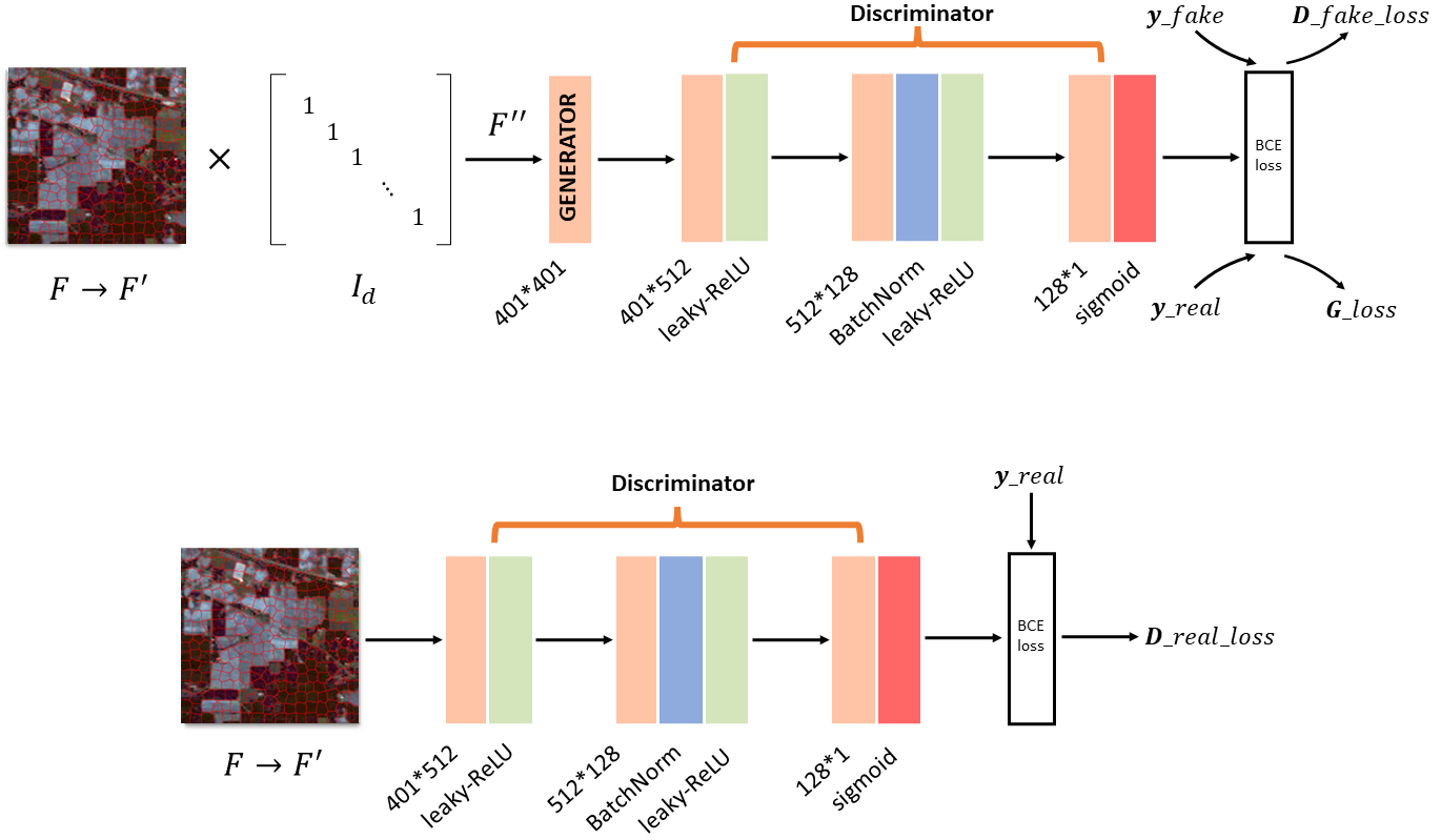
Figure 1: GAN-framework

III-B2 Feature Extraction

After the image preprocessing process, for the sample class $m_{i}$, we mark the number of superpixel blocks in the class as $b_{m}$, and the feature vector of superpixel block as $f_{m}^{j}\in\mathbbm{R}^{(1\times d)},j\in[0,b_{m})$, $d$ represents the dimension of the feature vector after preprocessing. We filter out the maximum amounts of superpixel blocks in the classes as $(b_{m})_{max}$. For the class $m_{i}$ which meets the conditions of $b_{m_{i}}<0.02\times(b_{m})_{max}$, we define it as minority class, extract its feature vectors $f_{m_{i}}^{j}$ and splice it vertically into a minority class feature matrix $\mathbb{F}_{i}\in\mathbbm{R}^{b_{m_{i}}\times d}.$

Due to the high spectral dimension of the feature matrix, the existing mainstream spectral feature extraction methods and minority class data generation strategies are usually performed by applying PCA method [5], which leads to the loss of effective information. As a result, it reduces the classification accuracy of the model.

In order to achieve a balance between generation efficiency and data diversity, we design a transition matrix optimization strategy based on adversarial methods, we use the original feature vector as the input of the discriminator and train the discriminator’s ability to identify minority class feature vectors. The feature matrix perturbed by the transition matrix is imported into the generator, then we input the generated result into the discriminator. The generator and discriminator are trained respectively. We assume that the weight matrix of the generator is $\mathbb{W}_{\bm{G}}$, in order to realize the perturbation operation on the original feature matrix, it is necessary to initialize the $mean(\mathbb{W}_{\bm{G}})=1$, and set a small variance to adapt to the data characteristic of the preprocessed feature matrix.

III-B3 Feature Enhancement

For the purpose of cooperating with the optimization strategy designed, we construct a feature enhancement algorithm for minority class sequence data. For the minority class feature matrix $\mathbb{F}_{i}$ generated from preprocessing, we replicate it longitudinally to $d$-dimension and get $\mathbb{F}_{i}^{\prime}$, we import it into the discriminator as real data for training. We perform the operation $\mathbb{F}_{i}^{\prime\prime}=\mathbb{F}_{i}^{\prime}\times\mathbb{I}_{d}$ and do the perturbation to matrix $\mathbb{F}_{i}^{\prime\prime}$ with generator. Through this process, we construct a diagonal feature matrix that can be input into the generator for convolution, and the output of the generator has the characteristic that each row is a slice of new generated feature vector. By mixing in order, we effectively increase the data diversity of the training set. At the same time, if the replication order of the original feature matrix $\mathbb{F}_{i}$ to generate the feature matrix is adjusted, we will get different forms of enhanced features vector, which greatly reduces the overfitting probability of the model.

III-B4 Loss Function

We design the loss function of the data augmentation model by inheriting the form of the GAN network loss function. To set an example, we only perform the data enhancement operation to a single class and ignore the mark of $i$, we define $\bm{y}_{real}$ and $\bm{y}_{fake}$ which have all elements equal to 1 and 0 with a proper size. First we calculate the training loss $\bm{G}_{loss}$ of the generator

$$\bm{G}_{loss}=BCE\_loss(\bm{D}(\bm{G}(\mathbb{F}^{\prime}\otimes\mathbb{I}),\bm{y}_{real}),$$ (5)

in which the $BCE\_loss$ refers to the binary cross entropy loss function, then input the original data and the generated data into the discriminator. Training loss $\bm{D}_{loss}$ with following equations:

$$\bm{D}_{real\_loss} =BCE\_loss(\bm{D}(\mathbb{F}),\bm{y}_{real})$$ (6)

$$\bm{D}_{fake\_loss} =BCE\_loss(\bm{D}(\bm{G}(\mathbb{F}^{\prime}\otimes\mathbb{I}),\bm{y}_{fake})$$ (7)

$$\bm{D}_{loss} =\bm{D}_{real\_loss}+\bm{D}_{fake\_loss}.$$ (8)

We define the final loss function as follows:

$$\min_{\bm{G}}\max_{\bm{D}}V(\bm{D},\bm{G})=\bm{G}_{loss}-\bm{D}_{loss}.$$ (9)

After the training process, we take the output of the generator filling into the original feature matrix according to the model learning requirements, so as to realize the data enhancement for the minority class.

III-C Bayesian Layer and BLGCN

III-C1 Bayesian Deep Learning

In general, for a Bayesian deep neural network, its predicted value can be calculated by Eq. 2, and the calculation depends on the approximate inference of the posterior distribution $p(y^{*}\mid x^{*},\bm{Y},\bm{X})$ expressed in Eq. 3. We take the approach of variational inference and use a simple distribution $q(\omega)$ to approximate the posterior distribution $p(\omega\mid\bm{Y},\bm{X}).$

In order to make $q(\omega)$ fit $p(\omega\mid\bm{Y},\bm{X})$ as closely as possible, we only need to minimize Kullback–Leibler divergence $KL[q(\omega)\parallel p(\omega\mid\bm{Y},\bm{X})]$ [44].

To present uncertainty, we assume that both the approximate posterior and the prior follow Gaussian distribution, i.e.,

$$q(\omega)=q(\omega\mid\theta),\theta=(\mu,\sigma)$$ (10)

$$p(\omega_{i}\mid\bm{Y},\bm{X})\sim\mathbbm{N}(\omega_{i}\mid\mu_{i},{\sigma_{i}}^{2}).$$ (11)

The original problem can be transformed into optimizing the parameter

$$\theta^{*} =\mathop{\arg\min}_{\theta}KL[q(\omega\mid\theta)\parallel p(\omega\mid\bm{Y},\bm{X}))]$$ (12)

$$=\mathop{\arg\min}_{\theta}\mathbbm{E}_{q(\omega\mid\theta)}[\log\frac{q(\omega\mid\theta)}{p(\omega\mid\bm{Y},\bm{X})}]$$

$$=\mathop{\arg\min}_{\theta}\mathbbm{E}_{q(\omega\mid\theta)}[\log\frac{q(\omega\mid\theta)p(\bm{Y}\mid\bm{X})}{p(\omega\mid\bm{Y},\bm{X})p(\omega)}]$$

$$=\mathop{\arg\min}_{\theta}\mathbbm{E}_{q(\omega\mid\theta)}[\log\frac{q(\omega\mid\theta)}{p(\bm{Y}\mid\bm{X},\omega)p(\omega)}]$$

and expressed as minimizing the loss function

$$Loss=KL[q(\omega\mid\theta)\parallel p(\omega)]-\mathbbm{E}_{q(\omega)}\log(p(\bm{Y}\mid\bm{X},\omega)).$$ (13)

We apply the reparameter trick here [45], for the weights $\omega_{i}\sim\mathbbm{N}(\mu_{i},{\theta_{i}}^{2})$, we have $\omega_{i}=\mu_{i}+\theta_{i}\odot\epsilon_{i}$, where $\epsilon_{i}\sim\mathbbm{N}(0,1)$, and $\odot$ represents Hadamard product. Then for the backpropagation of the loss function Eq. 13, we have

$$\frac{\partial}{\partial\theta}\mathbbm{E}_{q(\epsilon)}\{\log[\frac{q(\omega\mid\theta)}{p(\bm{Y}\mid\bm{X},\omega)p(\omega)}]\}$$ (14)

$$=\mathbbm{E}_{q(\epsilon)}\{\frac{\partial}{\partial\theta}\log[\frac{q(\omega\mid\theta)}{p(\bm{Y}\mid\bm{X},\omega)p(\omega)}]\}.$$

In order to ensure that the range of parameter $\theta$ includes the entire real number axis, we need to perform the reparameter trick on it, with $\sigma=\log(1+e^{\rho})$ we have $\theta=(\mu,\rho).$

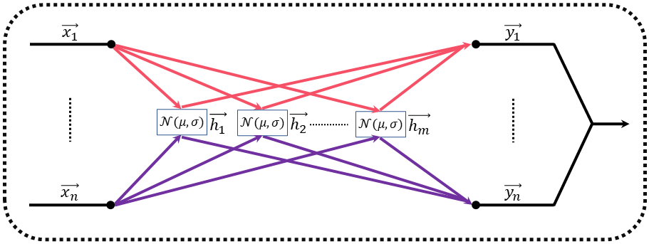
Figure 2: Bayesian Layer

III-C2 Bayesian Layer

The Bayesian neural network used in the current research field is relatively fixed in form, and has not been effectively combined with the convolutional neural network [45]. Researchers usually simply migrate the Bayesian forward propagation method and loss function to the traditional neural networks, and ignore adjusting the network structure in combination with specific tasks. Since the weight matrix of Bayesian neural network obeys a specific distribution, whether it is dealt with variable inference method or the MCMC method, we need to perform multiple sampling in the forward propagation with approximate calculation, which will take a great time cost. And when dealing with the hyperspectral image classification task, directly applying Bayesian theory to completely transform graph convolutional neural networks limits the room to fine-tune the network framework and improve the classification results.

Therefore, we propose the concept of Bayesian layer. We define the Bayesian layer as a convolutional layer which all weight parameters and biases are represented in distributed form as shown in Fig. 2. In the process of forward propagation, the input features matrix will be divided into several row vectors $\overrightarrow{x_{n}}$, and the Bayesian matrix can be seen as a set of column vectors $\overrightarrow{h_{n}}$, which is assembled by weight parameters of $\mu$ and $\theta$. In the matrix multiplication operation, we have $\overrightarrow{y_{nm}}=\overrightarrow{x_{n}}\times\overrightarrow{h_{m}}$.

At the same time, we stipulate that the loss function must have the form of KL divergence which can be optimized by the variational inference method. By analyzing the form of the Bayesian convolutional neural network loss function, we find that the likelihood function term can be replaced by a multi-classification loss. The reason is, given the model output $y$, the likelihood function $L(\omega\mid y)$ about the parameter $\omega$ is numerically equals to the probability $p(Y=y\mid\omega)$ of the output $y$ given the parameter $\omega$. In the process of each forward propagation, the weight parameters of the non-Bayesian layer remain unchanged when the Bayesian layer is sampled multiple times, so each time the gradient is updated in the backpropagation, the existence of non-Bayesian layer will not influence the derivation operation towards the Bayesian layer.

As a result, if we use the classification loss function of traditional neural network such as negative log-likelihood loss (nll loss) to represent the likelihood function, it can provide the theoretical basis for the realization of the Bayesian layer. Here we can rewrite Eq. 13 as follows:

$$\begin{split}Loss&=\sum_{i}\log{q(\omega_{i}\mid\theta_{i})}-\sum_{i}\log{p(\omega_{i})}\\ &-\sum_{j}\log{p(y_{j}\mid\omega,x_{j})}\\ &=\sum_{i}\log{q(\omega_{i}\mid\theta_{i})}-\sum_{i}\log{p(\omega_{i})}-nll\_loss.\end{split}$$ (15)

According to the former demonstration, when upgrading the weight parameters of a Bayesian layers convolutional neural network in gradient calculation and back propagation, we know that the prior distribution loss $\sum_{i}\log{p(\omega_{i})}$ and posterior distribution loss $\sum_{i}\log{q(\omega_{i}\mid\theta_{i})}$ only relate to the weights of Bayesian layer, and the multi-classification loss relates to all the weight parameters of the neural network. Therefore, the parameter updates of the Bayesian layer and the non-Bayesian layer can be performed sequentially under the same process without interfering with each other.

Meanwhile, it also gives us more choices in diversification. Facing various tasks, we can choose different insertion methods of the Bayesian layer, which can achieve the uncertainty quantization output while ensuring that the loss function structure of the original neural network is not damaged.

III-C3 BLGCN

We combine the idea of graph convolution with Bayesian layers, where the output of each Bayesian layer is multiplied with the preprocessed adjacency matrix to fuse the spatial features of hyperspectral images. More specifically, the adjacency matrix $\mathbb{A}$ got from the preprocessing is renormalized with the method proposed by Kipf&Welling [40]. To generalize the formulation of $\hat{\mathbb{A}}_{G}$, we perform the trick

$$\hat{\mathbb{A}}_{G}=\hat{\mathbb{D}}^{-\frac{1}{2}}\hat{\mathbb{A}}\hat{\mathbb{D}}^{-\frac{1}{2}}$$ (16)

with $\hat{\mathbb{A}}=\mathbb{A}+\mathbb{I}$ and $\hat{\mathbb{D}}_{ii}=\sum\nolimits_{j}\hat{\mathbb{A}}_{ij}$. Here, $\mathbb{I}$ denotes the identity matrix which has proper size to calculate. Hence, for each Bayesian layer, the output can be expressed with Eq. 1 after sampling on the weight parameter matrix.

The main framework of BLGCN is shown in Fig. 3, we set a feature extraction module before the two Bayesian layer modules, which consists of two full-connected convolutional layers and a ReLU layer, it can roughly extract the data features and provide a solid foundation for the Bayesian processing.

It should be noted that for the data-enhanced hyperspectral data, in order to maintain the consistency of the spatial information, the adjacency matrix needs to be expanded. We assume that the newly generated superpixels have similar spatial characteristics with the original superpixels of the same class. We randomly match the generated ones with those initial superpixels, and give them the same adjacency relationship with the matched ones, thereby regenerating a new adjacency matrix.

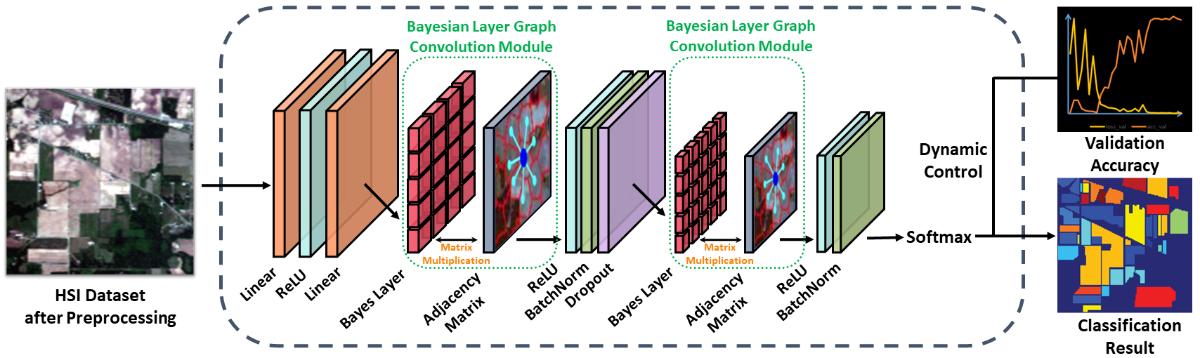
Figure 3: Bayesian layer graph convolutional network

III-D Training Strategy based on Bayesian Method

The prediction results given by deep learning models are not always reliable, and some application fields of hyperspectral image classification have high requirements for confidence. By modeling uncertainty with output variance, we dynamically evaluate the confidence level of the training results and make decisions on whether terminate the training process.

From the central limit theorem, we know that if the sample size is large enough, the sampling distribution can be approximated as a normal distribution. Due to the existence of the Bayesian layer, we can consider that outputs of the multiple times forward propagation after fixing the model are independent from each other. Therefore, by calculating the mean and variance of the multiple forward propagation output, we can obtain an interval estimate of the accuracy and a confidence interval under the premise of given confidence.

To enable dynamic evaluation of the training process, we set two accuracy thresholds and calculate the accuracy of the validation set after each training process. When it reaches the first threshold, the model weights are fixed after each training batch and the forward propagation is performed 30 times. We record the output results and calculate whether the confidence interval upper bound of the validation set accuracy reaches the second threshold we set under 95% confidence level, and if it does, the training will be stopped immediately. For training tasks with specific sample classification accuracy requirements, we only need to change the two judgment operations on the validation set accuracy to the specific class accuracy.

We applied statistical knowledge to calculate the confidence interval of the accuracy. For the case of large sample size, we used the Z-test to determine whether the sample mean was significantly different from the population mean. We first calculate the sample mean $\mu$ and standard error $SE$, then determine the confidence level and get the standard score $z$. When the confidence level is set to 95%, the standard score $z$ is numerically equal to 1.96, and the bounds of the confidence interval $[a,b]$ are shown in below:

$$a=\mu-\left|z\right|\times SE$$ (17)

$$b=\mu+\left|z\right|\times SE.$$

We combine the proposed model with dynamic control strategy, and formulate the whole classification process in forms of flow chart. The implementation details of the process are shown in Algorithm 1.

Algorithm 1 Proposed BLGCN with Dynamic Control Strategy for HSI Classification

$\mathbb{Input:}$ Input image; number of iterations $i$; Threshold $\bm{T_{1}}$,$\bm{T_{2}}$
  $\mathbb{Output:}$ Classification Result

1:// Preprocessing the dataset

2:Segment the input image into superpixels with SLIC;

3:Label the superpixels and exclude the background;

4:Construct the adjacency matrices $\bm{A}$;

5:Extract the image information into the feature matrix $\bm{F}$;

6:if The sample imbalance problem is serious then

7:     Train the GAN network on preprocessed dataset with Eq. 9;

8:     Expand the feature matrix $\bm{F}$ with generated data;

9:     Update the adjacency matrices $\bm{A}$;

10:// Training process with dynamic control

11:for epoch in range $i$ do

12:     Train the model with BLGCN with Eq. 15;

13:     if validation set accuracy reaches $\bm{T_{1}}$ then

14:         Fix the model;

15:         Perform the forward propagation 30 times;

16:         Calculate the confidence interval with Eq. 17;

17:         if confidence interval reaches $\bm{T_{2}}$ then

18:              Break               

19:return result.

IV Experimental Analysis

IV-A Dataset Description and Evaluation Criteria

In our experiment, we select four mainstream hyperspectral remote sensing datasets, including Indian Pines, Salinas, Pavia University and Houston University to verify the advantages of the model we proposed.

Indian Pines dataset was obtained by AirBorne Visible&Infrared Imaging Spectrometer sensor over the Indian Pines region in 1992. It contains 145$\times$145 pixels and consists of 220 spectral bands covering the range from 0.4 $\mu$m to 2.5 $\mu$m. 20 bands absorbed by water vapor are removed and the remaining 200 spectral bands are used for model classification. This dataset contains 16 kinds of landscapes. After the image preprocessing, the pixels in the dataset are aggregated into several superpixels. The number of superpixels in each landscape class and their corresponding training and testing samples are listed in Table I. The ground-truth map is shown in Fig. 4.

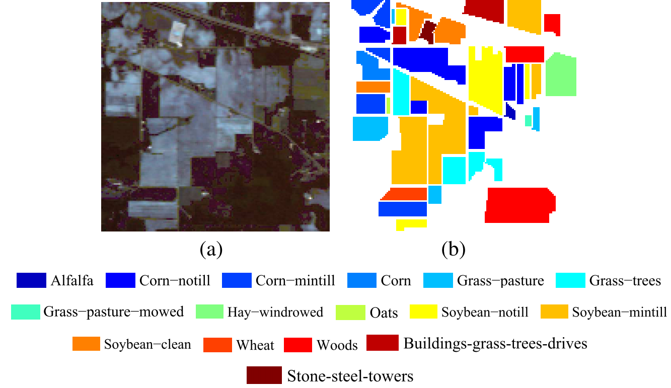
Figure 4: Indian Pines. (a) False color image. (b) Ground truth map.

TABLE I:
NUMBERS OF LABELED AND UNLABELED SUPERPIXELS USED IN THE INDIAN PINES DATASET

ID		Class	Labeled	Unlabeled
1		Alfalfa	5	41
2		Corn-notill	143	1285
3		Corn-mintill	83	747
4		Corn	24	213
5		Grass-pasture	48	435
6		Grass-trees	73	657
7		Grass-pasture-mowed	3	25
8		Hay-windrowed	48	430
9		Oats	2	18
10		Soybean-notill	97	875
11		Soybean-mintill	246	2209
12		Soybean-clean	59	534
13		Wheat	21	185
14		Woods	127	1138
15		Buildings-grass-trees-drives	39	347
16		Stone-steel-towers	9	84

The University of Pavia dataset was acquired over the Pavia University in Italy in 2001. It contains 610$\times$340 pixels in 103 spectral bands and has a wavelength range from 0.43 $\mu$m to 0.86 $\mu$m after removing the noisy bands. Table III lists the details of the superpixels and the amounts of training and testing samples. Fig. 6 shows the ground-truth map of the dataset.

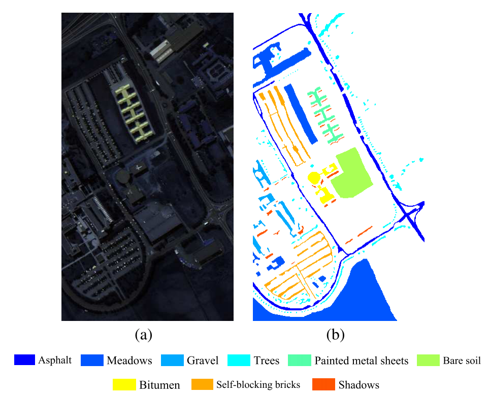
Figure 5: Pavia University. (a) False color image. (b) Ground truth map.

TABLE II:
NUMBERS OF LABELED AND UNLABELED SUPERPIXELS USED IN THE PAVIA UNIVERSITY

ID		Class	Labeled	Unlabeled
1		Asphalt	663	5968
2		Meadows	1854	16795
3		Gravel	210	1889
4		Trees	306	2758
5		Painted metal sheets	135	1210
6		Bare soil	503	4526
7		Bitumem	133	1197
8		Self-blocking bricks	368	3314
9		Shadows	95	852

Salinas dataset captured the Salinas Valley in California. This dataset contains 512$\times$127 pixels in 224 bands. 20 bands absorbed by water vapor are removed and the remaining 204 spectral bands are used for classification. Its ground-truth map is shown in Fig. 5 and the number of superpixels with their information are listed in Table II.

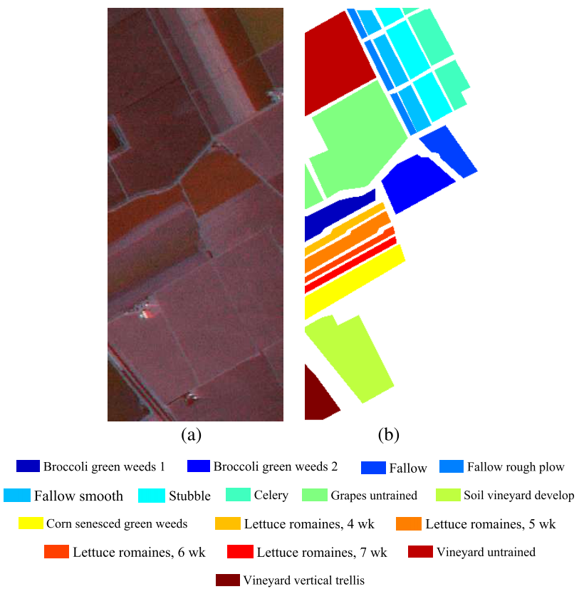
Figure 6: Salinas. (a) False color image. (b) Ground truth map.

TABLE III:
NUMBERS OF LABELED AND UNLABELED SUPERPIXELS USED IN THE SALINAS DATASET

ID		Class	Labeled	Unlabeled
1		Brocoli-green-weeds-1	201	1808
2		Brocoli-green-weeds-2	373	3353
3		Fallow	198	1778
4		Fallow-rough-plow	139	1255
5		Fallow-smooth	268	2410
6		Stubble	393	3536
7		Celery	358	3221
8		Grapes-untrained	1127	10144
9		Soil-vinyard-develope	620	5583
10		Corn-senesced-green-weeds	328	2950
11		Lettuce-romaine-4wk	107	961
12		Lettuce-romaine-5wk	193	1734
13		Lettuce-romaine-6wk	92	824
14		Lettuce-romaine-7wk	107	963
15		Vinyard-untrained	727	6541
16		Vinyard-vertical-trellis	181	1626

The University of Houston dataset is provided by the IEEE GRSS Data Fusion Contest in 2013. This dataset consists of 349$\times$1905 pixels and contains 144 spectral bands covering the range from 364 nm to 1046 nm. The number of superpixels in each landscape class and their corresponding training and testing samples are given in Table IV with its ground-truth map shown in Fig. 7.

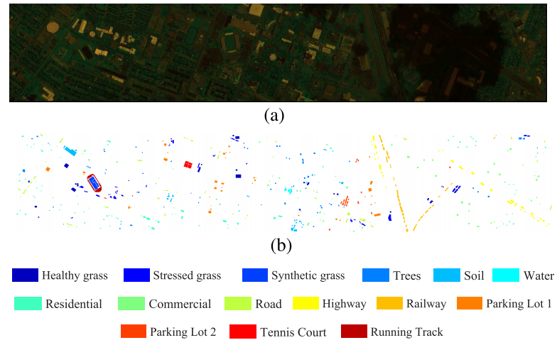
Figure 7: Houston University. (a) False color image. (b) Ground truth map.

TABLE IV:
NUMBERS OF LABELED AND UNLABELED SUPERPIXELS USED IN THE HOUSTON UNIVERSITY

ID		Class	Labeled	Unlabeled
1		Healthy grass	125	1126
2		Stressed grass	125	1129
3		Synthetic grass	70	627
4		Trees	124	1120
5		Soil	124	1118
6		Water	33	292
7		Residential	127	1141
8		Commercial	124	1120
9		Road	125	1127
10		Highway	123	1104
11		Railway	124	1111
12		Parking Lot1	123	1110
13		Parking Lot2	47	422
14		Tennis Court	43	385
15		Running track	66	594

In our experiment, four metrics are adopted to quantificationally evaluate the classification performance which are per-class accuracy, overall accuracy (OA), average accuracy (AA), and kappa coefficient (Kappa).

IV-B Experimental Settings

In our experiment, the proposed model is implemented via Pytorch with the Adam optimizer. We train our model with 0.2 dropout rate, 5$\times 10^{-4}$ weight decay rate. We adopt the learning rate decay strategy in the training process. We set the initial learning rate as 1$\times 10^{-3}$ and use the multistep learning rate strategy with gamma fixed to 0.9, and three milestones are 1500, 2500 and 3500. The threshold parameter of assigning the pseudo label to the unlabeled nodes is set to 0.9, which means that besides the training sample, all the rest samples are distributed to the validation set.

In the SLIC algorithm in image preprocessing, we set the compactness parameter to 0.08 for all experiments. And in our GAN algorithm in data augment process, the initial standard deviation of the generator weight matrix and the discriminator weight matrix are set to 1$\times 10^{-5}$ and 0.01, respectively. Because of the data characteristics after the normalization operation in data preprocessing, the learning rate in our GAN network is set to 1${\times 10^{-7}}$. For the landscape class which has the superpixels sample size less than 0.02 times of the superpixels sample size of the largest class sample, we define it as minority class and perform the data augment process towards it, the generated samples are filled into the original dataset until the sample size of the minority class reaches the threshold of 0.05 times of the superpixels sample size of the largest class sample.

IV-C Classification Results

In order to evaluate the effectiveness of our proposed BLGCN model, we conduct comparative experiments with various comparison algorithms on the selected dataset. To make the experiment results reliable, various SOTA algorithms are selected as the competitors. Among the algorithms based on traditional machine learning, we selected the support vector machine algorithm (SVM) [52]. The commonly used SVM kernel includes linear kernel, polynomial kernel, Gaussian kernel and Sigmoid kernel. We make the SVM network search for optimization in the given parameter set, and then select the appropriate hyperparameters for the classification task. For convolutional neural network based on deep learning methods, we select the 3D-CNN convolutional neural network [53] which performs well over the HSI datasets. For graph convolutional neural network based model, we select several algorithms that have been widely used in recent years, such as GCN [40], spectral-spatial graph convolutional network (S²GCN) [31], and multiscale dynamic GCN (MDGCN) [29], etc. They are powered by the GCN idea to improve the network in a targeted manner, and have achieved better classification results on the HSI datasets. We perform 30 independent experiments on each dataset based on the algorithm chosen based on the application and recorded the mean and standard deviation of the results. It is worth noting that since the classification accuracies are quite poor when the 3D-CNN model is performed on the HSI datasets with 10% training set ratio, we only show the classification results with 30% training set ratio on the last three datasets.

The classification results on the Indian Pines dataset show the effectiveness of our algorithm. The traditional algorithm (SVM) and the original GCN have serious misclassification problem in the face of minority class categories classification task, and the accuracy of the 3D-CNN method based on full-supervised classification is also relatively low. When the proportion of training set samples is increased from 10% to 30%, the classification effect has been significantly improved. Compared with other GCN methods, our method has obvious advantages in the task of distinguishing minority class categories, i.e., Class 7 and Class 9, while maintaining high classification accuracy on other sample categories. The relevant results are listed in Table V.

TABLE V:
CLASSIFICATION RESULTS ON INDIAN PINES DATASET

Class		SVM	3D-CNN(0.1)	3D-CNN(0.3)	GCN	S2GCN	MDGCN	BLGCN
1		59.81$\pm$11.20	78.93$\pm$16.75	95.55$\pm$3.99	73.27$\pm$16.47	92.05$\pm$5.64	90.02$\pm$4.62	92.30$\pm$3.63
2		73.53$\pm$1.70	82.19$\pm$1.75	94.42$\pm$1.43	81.03$\pm$1.66	82.84$\pm$2.32	77.83$\pm$1.87	96.80$\pm$1.19
3		65.63$\pm$2.81	77.25$\pm$2.98	89.73$\pm$1.49	81.90$\pm$0.79	80.34$\pm$3.15	95.39$\pm$2.56	95.94$\pm$3.27
4		54.66$\pm$5.29	76.59$\pm$3.90	92.81$\pm$0.99	69.76$\pm$0.64	90.10$\pm$1.85	95.69$\pm$1.49	96.92$\pm$6.19
5		88.67$\pm$1.77	92.41$\pm$1.82	95.69$\pm$0.87	95.44$\pm$0.42	94.10$\pm$0.1	92.36$\pm$0.04	93.25$\pm$4.50
6		92.48$\pm$1.07	97.41$\pm$0.82	99.09$\pm$0.23	100.00$\pm$0.00	94.25$\pm$0.24	94.32$\pm$0.16	99.40$\pm$0.80
7		75.42$\pm$7.90	80.53$\pm$12.10	92.75$\pm$3.29	0.00$\pm$0.00	67.49$\pm$6.22	82.03$\pm$5.09	93.30$\pm$7.90
8		96.22$\pm$0.90	98.41$\pm$0.89	99.86$\pm$0.14	100.00$\pm$0.00	95.93$\pm$0.03	96.00$\pm$0.00	100.00$\pm$0.00
9		36.98$\pm$13.95	73.95$\pm$15.89	95.62$\pm$3.80	0.00$\pm$0.00	75.13$\pm$7.85	79.02$\pm$6.44	100.00$\pm$0.00
10		69.44$\pm$1.92	83.21$\pm$2.03	93.02$\pm$1.27	79.26$\pm$0.94	90.86$\pm$0.95	87.39$\pm$0.74	92.19$\pm$4.00
11		77.65$\pm$1.43	85.97$\pm$1.61	94.69$\pm$0.76	91.73$\pm$0.08	82.38$\pm$2.14	90.62$\pm$1.72	98.08$\pm$1.21
12		70.43$\pm$4.76	80.17$\pm$3.01	93.77$\pm$1.11	86.66$\pm$1.20	77.62$\pm$4.79	90.33$\pm$3.91	97.94$\pm$3.29
13		94.12$\pm$2.11	97.57$\pm$1.51	99.29$\pm$0.44	93.14$\pm$2.80	96.32$\pm$0.72	97.08$\pm$0.55	99.86$\pm$0.33
14		93.85$\pm$0.71	96.15$\pm$0.95	98.73$\pm$0.34	97.37$\pm$0.98	93.71$\pm$1.45	96.81$\pm$1.15	99.72$\pm$0.82
15		59.32$\pm$3.54	73.52$\pm$3.76	87.91$\pm$1.44	86.86$\pm$0.60	84.13$\pm$1.18	96.81$\pm$0.93	95.07$\pm$3.12
16		94.34$\pm$2.33	96.64$\pm$2.13	99.00$\pm$0.62	96.14$\pm$1.70	96.87$\pm$1.18	92.91$\pm$0.00	100.00$\pm$0.00
OA		78.78$\pm$1.03	86.08$\pm$0.77	94.24$\pm$0.58	88.80$\pm$0.53	84.91$\pm$1.79	87.09$\pm$1.33	97.22$\pm$0.81
AA		75.09$\pm$3.93	85.62$\pm$2.38	95.26$\pm$0.44	75.97$\pm$0.45	87.08$\pm$2.23	90.25$\pm$1.98	97.02$\pm$1.15
Kappa		75.70$\pm$1.20	84.14$\pm$0.87	93.46$\pm$0.68	87.21$\pm$0.57	83.02$\pm$0.98	86.53$\pm$0.86	96.81$\pm$0.94

Table VI shows the classification effects of different algorithms on the Pavia University dataset. Among these methods, the algorithm we proposed still maintains the highest classification accuracy, and has achieved 100% recognition and classification accuracy in several categories. It is worth noting that due to the relatively balanced sample size of the PU dataset, the 3D-CNN model also reaches a good classification effect after we increase the training set ratio to 30%, and gets the highest classification accuracy in some categories. For the samples class that are scattered in spatial such as Class 4, the classification methods based on GCN fail to achieve good results. The main reason is that its spatial adjacency relationship is relatively sparse, and makes it easy to be misclassified when using the GCN methods.

TABLE VI:
CLASSIFICATION RESULTS ON PAVIA UNIVERSITY DATASET

Class		SVM	3D-CNN(0.3)	GCN	S2GCN	MDGCN	BLGCN
1		92.40$\pm$1.71	97.94$\pm$0.10	70.97$\pm$0.57	90.69$\pm$1.84	91.09$\pm$0.45	96.45$\pm$4.34
2		95.54$\pm$0.84	97.44$\pm$0.05	96.55$\pm$0.28	85.02$\pm$3.22	96.64$\pm$0.41	99.12$\pm$0.75
3		79.92$\pm$1.23	94.56$\pm$0.26	24.74$\pm$0.55	85.91$\pm$3.18	89.61$\pm$0.29	83.25$\pm$11.57
4		93.70$\pm$2.17	98.02$\pm$0.13	47.25$\pm$1.61	88.72$\pm$1.24	81.57$\pm$1.97	66.76$\pm$1.49
5		99.55$\pm$0.22	99.88$\pm$0.04	100.00$\pm$0.00	97.66$\pm$0.98	96.86$\pm$0.21	100.00$\pm$0.00
6		85.61$\pm$2.29	98.26$\pm$0.19	99.95$\pm$0.15	86.52$\pm$1.59	92.75$\pm$0.48	100.00$\pm$0.00
7		76.53$\pm$8.90	98.36$\pm$0.09	94.24$\pm$1.39	96.57$\pm$0.76	96.32$\pm$1.26	98.00$\pm$2.58
8		86.22$\pm$1.10	96.52$\pm$0.37	100.00$\pm$0.00	87.86$\pm$3.01	92.49$\pm$1.00	91.71$\pm$1.83
9		99.90$\pm$1.41	99.68$\pm$0.11	0.00$\pm$0.00	96.58$\pm$0.79	78.89$\pm$0.78	100.00$\pm$0.00
OA		91.96$\pm$1.41	96.58$\pm$0.04	90.84$\pm$0.19	87.64$\pm$1.82	93.16$\pm$0.26	97.56$\pm$0.38
AA		89.82$\pm$0.28	97.80$\pm$0.05	80.37$\pm$0.33	90.70$\pm$0.65	90.70$\pm$0.74	91.42$\pm$2.21
Kappa		89.20$\pm$1.80	95.44$\pm$0.05	85.40$\pm$0.27	84.66$\pm$1.97	91.77$\pm$0.39	96.15$\pm$0.73

The classification results we get on the Salinas dataset are listed in Table VII. Compared with other algorithms, BLGCN basically achieves the highest classification accuracy in all categories, while maintaining high stability. We find that the SVM method also has higher classification accuracy than the deep learning algorithm, which shows that there is also room for the application of traditional classification methods in datasets with sufficient and balanced sample data such as Salinas.

TABLE VII:
CLASSIFICATION RESULTS ON SALINAS DATASET

Class		SVM	3D-CNN(0.3)	GCN	S2GCN	MDGCN	BLGCN
1		98.80$\pm$0.10	98.38$\pm$0.04	97.44$\pm$0.55	97.90$\pm$0.43	98.26$\pm$0.02	100.00$\pm$0.00
2		99.80$\pm$0.11	98.88$\pm$0.06	99.94$\pm$0.13	98.07$\pm$0.29	98.18$\pm$0.13	100.00$\pm$0.00
3		98.94$\pm$0.51	99.19$\pm$0.32	96.88$\pm$2.42	96.06$\pm$0.55	98.08$\pm$0.15	100.00$\pm$0.00
4		99.25$\pm$0.16	99.38$\pm$0.17	97.42$\pm$0.62	97.99$\pm$0.51	95.81$\pm$0.87	100.00$\pm$0.00
5		99.00$\pm$0.00	99.11$\pm$0.38	89.53$\pm$0.17	96.46$\pm$0.60	96.27$\pm$1.32	99.11$\pm$1.04
6		99.91$\pm$0.12	99.55$\pm$0.05	100.00$\pm$0.00	98.21$\pm$0.19	97.40$\pm$1.02	100.00$\pm$0.00
7		99.88$\pm$0.15	99.50$\pm$0.11	99.72$\pm$0.27	97.95$\pm$0.24	96.49$\pm$1.56	100.00$\pm$0.00
8		84.77$\pm$0.24	77.78$\pm$11.49	97.68$\pm$0.43	69.88$\pm$5.89	91.18$\pm$2.96	99.19$\pm$1.04
9		99.56$\pm$0.10	99.75$\pm$0.05	99.42$\pm$0.01	97.22$\pm$0.97	98.28$\pm$0.79	100.00$\pm$0.00
10		96.23$\pm$0.63	97.57$\pm$0.05	95.84$\pm$0.49	89.95$\pm$2.41	96.62$\pm$1.69	97.67$\pm$1.93
11		97.81$\pm$1.24	97.66$\pm$0.50	99.08$\pm$1.94	96.90$\pm$1.66	97.68$\pm$2.04	99.55$\pm$0.63
12		97.41$\pm$0.61	98.69$\pm$0.12	100.00$\pm$0.00	98.44$\pm$0.96	97.39$\pm$2.57	100.00$\pm$0.00
13		99.31$\pm$0.60	98.61$\pm$0.68	100.00$\pm$0.00	96.73$\pm$1.02	95.91$\pm$3.19	100.00$\pm$0.00
14		97.41$\pm$0.64	97.86$\pm$0.93	95.72$\pm$4.65	94.67$\pm$1.87	96.23$\pm$0.89	98.97$\pm$0.00
15		71.80$\pm$0.81	76.68$\pm$5.87	75.94$\pm$9.67	69.56$\pm$3.58	94.06$\pm$2.09	91.79$\pm$1.22
16		99.21$\pm$0.21	94.47$\pm$0.18	93.69$\pm$3.79	95.81$\pm$1.03	95.58$\pm$1.45	94.32$\pm$8.00
OA		92.63$\pm$1.71	91.03$\pm$3.10	94.75$\pm$1.66	87.40$\pm$1.24	96.52$\pm$2.81	98.30$\pm$0.22
AA		95.90$\pm$0.03	95.88$\pm$1.09	96.22$\pm$1.33	93.14$\pm$0.10	96.52$\pm$0.92	99.02$\pm$0.24
Kappa		91.80$\pm$0.20	90.05$\pm$3.39	94.13$\pm$1.86	86.12$\pm$2.01	95.27$\pm$0.96	98.10$\pm$0.25

We also apply BLGCN on the Houston University dataset to compare the classification efficiency. As we can see from Table VIII, the algorithm proposed in this paper greatly improves the classification accuracy, has obvious advantages over other algorithms, and has high classification performance on various sample classes. Besides, the comparison algorithms based on GCN have the problem that the classification accuracies on the majority samples classes such as Class 7 $\sim$ 12 are relatively low due to the minor ratio of training set samples. Because of the strong generalization ability in Bayesian layer, our model alleviates this problem successfully.

TABLE VIII:
CLASSIFICATION RESULTS ON HOUSTON UNIVERSITY DATASET

Class		SVM	3D-CNN(0.3)	GCN	S2GCN	MDGCN	BLGCN
1		95.80$\pm$0.60	98.88$\pm$0.44	81.07$\pm$0.00	95.41$\pm$2.03	92.72$\pm$0.97	99.58$\pm$0.70
2		97.41$\pm$0.51	98.84$\pm$0.38	100.00$\pm$0.00	97.66$\pm$1.08	92.97$\pm$0.78	99.34$\pm$0.06
3		99.25$\pm$0.48	99.42$\pm$0.44	74.89$\pm$2.21	97.97$\pm$1.35	97.39$\pm$0.60	100.00$\pm$0.00
4		96.83$\pm$0.75	99.30$\pm$0.35	89.24$\pm$0.00	96.78$\pm$1.14	94.87$\pm$1.05	100.00$\pm$0.00
5		95.44$\pm$1.41	99.38$\pm$0.29	92.34$\pm$3.97	96.76$\pm$0.97	98.27$\pm$0.32	99.97$\pm$0.06
6		96.16$\pm$2.59	96.44$\pm$2.26	86.90$\pm$0.00	95.95$\pm$1.45	92.58$\pm$1.14	98.23$\pm$1.71
7		83.21$\pm$1.84	93.26$\pm$0.89	51.54$\pm$1.43	82.71$\pm$3.54	87.01$\pm$2.28	97.91$\pm$0.96
8		72.74$\pm$1.72	94.56$\pm$2.89	90.73$\pm$0.00	75.44$\pm$4.11	79.83$\pm$4.07	94.82$\pm$1.71
9		76.51$\pm$1.21	90.02$\pm$0.76	32.06$\pm$7.07	81.41$\pm$2.69	88.96$\pm$0.19	92.97$\pm$2.56
10		81.32$\pm$1.40	91.90$\pm$0.47	65.99$\pm$2.96	86.05$\pm$2.01	89.38$\pm$1.70	99.83$\pm$0.07
11		81.74$\pm$1.26	92.92$\pm$0.86	62.56$\pm$2.42	87.75$\pm$2.00	86.07$\pm$1.64	98.62$\pm$0.92
12		69.19$\pm$1.82	91.24$\pm$2.09	70.63$\pm$3.68	77.91$\pm$4.68	88.76$\pm$2.97	99.69$\pm$0.30
13		48.51$\pm$6.95	98.94$\pm$4.48	0.00$\pm$0.00	74.93$\pm$4.26	92.08$\pm$1.02	96.49$\pm$1.29
14		96.25$\pm$1.47	98.94$\pm$0.34	98.88$\pm$2.51	98.53$\pm$0.44	98.69$\pm$0.39	100.00$\pm$0.00
15		98.08$\pm$0.51	98.80$\pm$0.48	72.44$\pm$4.62	97.13$\pm$0.68	95.55$\pm$0.44	100.00$\pm$0.00
OA		85.67$\pm$0.43	95.14$\pm$0.51	72.93$\pm$0.44	88.49$\pm$1.57	90.71$\pm$1.00	98.36$\pm$0.32
AA		86.28$\pm$0.96	95.60$\pm$0.71	70.44$\pm$0.54	89.50$\pm$1.04	91.68$\pm$1.07	98.30$\pm$0.40
Kappa		84.71$\pm$0.51	94.74$\pm$0.53	71.73$\pm$0.47	87.62$\pm$1.46	90.02$\pm$0.89	98.23$\pm$0.35

IV-D Ablation Study

We design ablation experiments for multiple functional modules implemented in BLGCN, and verify the necessity of each module in order to achieve high accuracy in classification. It is also been validated that dynamic control effects by processing the Indian Pines dataset.

IV-D1 Graph convolution operation

By using the method of graph convolution, our algorithm effectively extracts the spatial adjacency relationship between the superpixels of hyperspectral images, which greatly improves the classification efficiency. Among our method, the key operation of extracting the spatial relationship is the convolution operation of the feature matrix and the adjacency matrix. Therefore, we verify the necessity of the graph convolution module by removing the adjacency matrix convolution operation. The relevant comparison results are listed in Table IX. We can find that after removing the graph convolution operation, the overall classification results are greatly affected, and the accuracy rates have dropped significantly.

IV-D2 Minority class data generation module

Facing the problem of low accuracy in minority class classification that often occurs in practical classification tasks, this algorithm combines the generative adversarial network method to achieve effective expansion of minority classes. Therefore, we design a comparative experiment of removing the minority generation module and directly input the original data into the classification module. We list the results of the experiments in Table IX, in which the classification accuracies of the minority class 1, 7, and class 9 have dropped significantly after the minority class data generation module is removed, and they cannot be effectively classified at all.

IV-D3 Dynamic control training module guided by confidence intervals

Due to the uncertainty of the Bayesian neural network itself, we combine this feature to quantify the output uncertainty by calculating the confidence interval of the classification result, and dynamically control the training process whether to proceed. We design a comparative experiment on this module by removing the uncertainty calculation of the BLGCN classification results and the two thresholds in the training process, and we plot the correspondence between the accuracy of the validation set and the training batch in Fig. 8. It is shown that when given a 95% confidence level, the model automatically stops learning when the confidence interval reaches the second threshold, which saves plenty of training time.

TABLE IX:
ABLATION STUDY RESULTS ON INDIAN PINES DATASET

Class		BLGCN without GCN	BLGCN without GAN	BLGCN
1		0.00$\pm$0.00	0.00$\pm$0.00	92.30$\pm$3.63
2		72.82$\pm$18.21	94.05$\pm$7.43	96.80$\pm$1.19
3		59.58$\pm$21.11	92.45$\pm$3.12	95.94$\pm$3.27
4		49.04$\pm$15.69	98.44$\pm$1.00	96.92$\pm$6.19
5		89.76$\pm$2.87	96.85$\pm$1.42	93.26$\pm$4.50
6		94.38$\pm$2.50	99.77$\pm$0.50	99.40$\pm$0.80
7		0.82$\pm$1.73	0.00$\pm$0.00	93.30$\pm$7.91
8		95.90$\pm$3.71	100.00$\pm$0.00	100.00$\pm$0.00
9		17.50$\pm$28.09	0.00$\pm$0.00	100.00$\pm$0.00
10		57.64$\pm$30.88	84.42$\pm$4.68	92.19$\pm$4.00
11		69.82$\pm$15.07	94.39$\pm$9.73	98.08$\pm$1.21
12		69.54$\pm$5.62	94.67$\pm$6.39	97.94$\pm$3.28
13		96.32$\pm$2.86	100.00$\pm$0.00	99.86$\pm$0.33
14		97.37$\pm$0.50	100.00$\pm$0.00	99.72$\pm$0.82
15		44.52$\pm$1.60	90.81$\pm$2.16	95.07$\pm$3.12
16		90.32$\pm$4.91	100.00$\pm$0.00	100.00$\pm$0.00
OA		74.28$\pm$4.41	94.08$\pm$2.19	97.22$\pm$0.81
AA		65.36$\pm$3.17	81.85$\pm$0.95	97.02$\pm$1.16
Kappa		70.70$\pm$4.74	93.23$\pm$2.48	96.81$\pm$0.94

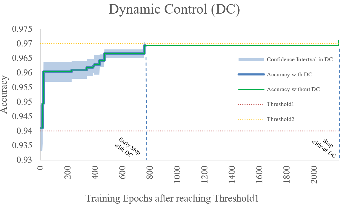
Figure 8: Ablation Study of Dynamic Control

V Conclusion

In this paper, we propose a novel BLGCN method for HSI classification. The proposed Bayesian layer is applied to the GCN-based networks to quantify the uncertainty of the output results. Since the distribution form is presented on only a few parts of the network, the proposed method maintains high classification accuracy and generalization ability. Meanwhile, newly designed GANs on minority class data are trained to enlarge its capacity and solve the sample imbalance problem in HSI dataset. To improve the training efficiency, a dynamic control strategy is designed for an early termination of the training process when the confidence interval reaches the threshold. The experimental results on four open source HSI datasets demonstrate the superiority of our proposed BLGCN. In addition, ablation studies are arranged to verify the contribution of different modules including graph convolution operation, data generation module and dynamic control strategy.

In the future, further research will be implemented on the various application field of Bayesian layer, including image classification and graph node prediction. Moreover, we will continue to improve the theoretical basis of Bayesian layer and make it available to various neural networks.

References

- [1] L. He, J. Li, C. Liu, and S. Li, “Recent advances on spectral–spatial hyperspectral image classification: An overview and new guidelines,” IEEE Trans. Geosci. Remote Sens., vol. 56, no. 3, pp. 1579–1597, Mar. 2018.
- [2] X. X. Zhu, D. Tuia, L. Mou, G.-S. Xia, L. Zhang, F. Xu, and F. Fraundorfer, “Deep learning in remote sensing: A comprehensive review and list of resources,” IEEE Geosci. Remote Sens. Mag., vol. 5, no. 4, pp. 8–36, Dec. 2017.
- [3] L. Zhang, L. Zhang, and B. Du, “Deep learning for remote sensing data: A technical tutorial on the state of the art,” IEEE Geosci. Remote Sens. Mag., vol. 4, no. 2, pp. 22–40, Jun. 2016.
- [4] C.-I. Chang, Hyperspectral data exploitation: theory and applications. John Wiley & Sons, 2007.
- [5] J. Shlens, “A tutorial on principal component analysis,” arXiv preprint arXiv:1404.1100, 2014.
- [6] M. Dalla Mura, A. Villa, J. A. Benediktsson, J. Chanussot, and L. Bruzzone, “Classification of hyperspectral images by using extended morphological attribute profiles and independent component analysis,” IEEE Geosci. Remote Sens. Lett., vol. 8, no. 3, pp. 542–546, May. 2011.
- [7] S. T. Roweis and L. K. Saul, “Nonlinear dimensionality reduction by locally linear embedding.” Science, vol. 290, no. 5500, p. 2323, Dec. 2000.
- [8] X. He and P. Niyogi, “Locality preserving projections,” in Proc. 28th Int. Conf. Neural Inf. Process. Syst., 2004, pp. 153–160.
- [9] W. R. Tobler, “A computer movie simulating urban growth in the detroit region,” Econ. Geography, vol. 46, pp. 234–240, Jun. 1970.
- [10] B. Zhang, S. Li, X. Jia, L. Gao, and M. Peng, “Adaptive markov random field approach for classification of hyperspectral imagery,” IEEE Geosci. Remote Sens. Lett., vol. 8, no. 5, pp. 973–977, Sep. 2011.
- [11] L. Sun, Z. Wu, J. Liu, L. Xiao, and Z. Wei, “Supervised spectral–spatial hyperspectral image classification with weighted markov random fields,” IEEE Trans. Geosci. Remote Sens., vol. 53, no. 3, pp. 1490–1503, Mar. 2015.
- [12] P. Zhong and R. Wang, “Modeling and classifying hyperspectral imagery by crfs with sparse higher order potentials,” IEEE Trans. Geosci. Remote Sens., vol. 49, no. 2, pp. 688–705, Feb. 2011.
- [13] F. Li, L. Xu, P. Siva, A. Wong, and D. A. Clausi, “Hyperspectral image classification with limited labeled training samples using enhanced ensemble learning and conditional random fields,” IEEE J. Sel. Topics Appl. Earth Observ., vol. 8, no. 6, pp. 2427–2438, Jun. 2015.
- [14] J. Zhao, Y. Zhong, Y. Wu, L. Zhang, and H. Shu, “Sub-pixel mapping based on conditional random fields for hyperspectral remote sensing imagery,” IEEE J. Sel. Topics Appl. Earth Observ., vol. 9, no. 6, pp. 1049–1060, Sep. 2015.
- [15] A. Plaza, P. Martinez, R. Perez, and J. Plaza, “A new approach to mixed pixel classification of hyperspectral imagery based on extended morphological profiles,” Pattern Recognit., vol. 37, no. 6, pp. 1097–1116, 2004.
- [16] J. Li, X. Huang, P. Gamba, J. M. Bioucas-Dias, L. Zhang, J. A. Benediktsson, and A. Plaza, “Multiple feature learning for hyperspectral image classification,” IEEE Trans. Geosci. Remote Sens., vol. 53, no. 3, pp. 1592–1606, Mar. 2015.
- [17] B. Demir and L. Bruzzone, “Histogram-based attribute profiles for classification of very high resolution remote sensing images,” IEEE Trans. Geosci. Remote Sens., vol. 54, no. 4, pp. 2096–2107, Apr. 2016.
- [18] Y. Chen, Z. Lin, X. Zhao, G. Wang, and Y. Gu, “Deep learning-based classification of hyperspectral data,” IEEE J. Sel. Topics Appl. Earth Observ., vol. 7, no. 6, pp. 2094–2107, Jun. 2014.
- [19] Y. Chen, X. Zhao, and X. Jia, “Spectral–spatial classification of hyperspectral data based on deep belief network,” IEEE J. Sel. Topics Appl. Earth Observ., vol. 8, no. 6, pp. 2381–2392, Jun. 2015.
- [20] Y. Chen, H. Jiang, C. Li, X. Jia, and P. Ghamisi, “Deep feature extraction and classification of hyperspectral images based on convolutional neural networks,” IEEE Trans. Geosci. Remote Sens., vol. 54, no. 10, pp. 6232–6251, Oct. 2016.
- [21] H. Lee and H. Kwon, “Going deeper with contextual cnn for hyperspectral image classification,” IEEE Trans. Image Process., vol. 26, no. 10, pp. 4843–4855, Otc. 2017.
- [22] M. Zhang, W. Li, and Q. Du, “Diverse region-based cnn for hyperspectral image classification,” IEEE Trans. Image Process., vol. 27, no. 6, pp. 2623–2634, Jun. 2018.
- [23] Z. Gong, P. Zhong, Y. Yu, W. Hu, and S. Li, “A cnn with multiscale convolution and diversified metric for hyperspectral image classification,” IEEE Trans. Geosci. Remote Sens., vol. 57, no. 6, pp. 3599–3618, Jun. 2019.
- [24] W. Li, G. Wu, F. Zhang, and Q. Du, “Hyperspectral image classification using deep pixel-pair features,” IEEE Trans. Geosci. Remote Sens., vol. 55, no. 2, pp. 844–853, Feb. 2017.
- [25] A. Romero, C. Gatta, and G. Camps-Valls, “Unsupervised deep feature extraction for remote sensing image classification,” IEEE Trans. Geosci. Remote Sens., vol. 54, no. 3, pp. 1349–1362, Mar. 2016.
- [26] L. Mou, P. Ghamisi, and X. X. Zhu, “Unsupervised spectral–spatial feature learning via deep residual conv–deconv network for hyperspectral image classification,” IEEE Trans. Geosci. Remote Sens., vol. 56, no. 1, pp. 391–406, Jan. 2018.
- [27] M. Zhang, M. Gong, Y. Mao, J. Li, and Y. Wu, “Unsupervised feature extraction in hyperspectral images based on wasserstein generative adversarial network,” IEEE Trans. Geosci. Remote Sens., vol. 57, no. 5, pp. 2669–2688, May. 2019.
- [28] P. Sellars, A. I. Aviles-Rivero, and C.-B. Schönlieb, “Superpixel contracted graph-based learning for hyperspectral image classification,” IEEE Trans. Geosci. Remote Sens., vol. 58, no. 6, pp. 4180–4193, Jan. 2020.
- [29] S. Wan, C. Gong, P. Zhong, B. Du, L. Zhang, and J. Yang, “Multiscale dynamic graph convolutional network for hyperspectral image classification,” IEEE Trans. Geosci. Remote Sens., vol. 58, no. 5, pp. 3162–3177, Nov. 2019.
- [30] S. Wan, C. Gong, P. Zhong, S. Pan, G. Li, and J. Yang, “Hyperspectral image classification with context-aware dynamic graph convolutional network,” IEEE Trans. Geosci. Remote Sens., vol. 59, no. 1, pp. 597–612, May. 2020.
- [31] A. Qin, Z. Shang, J. Tian, Y. Wang, T. Zhang, and Y. Y. Tang, “Spectral–spatial graph convolutional networks for semisupervised hyperspectral image classification,” IEEE Trans. Geosci. Remote Sens., vol. 16, no. 2, pp. 241–245, Sep. 2018.
- [32] L. Mou, X. Lu, X. Li, and X. X. Zhu, “Nonlocal graph convolutional networks for hyperspectral image classification,” IEEE Trans. Geosci. Remote Sens., vol. 58, no. 12, pp. 8246–8257, May. 2020.
- [33] X. He, Y. Chen, and P. Ghamisi, “Dual graph convolutional network for hyperspectral image classification with limited training samples,” IEEE Trans. Geosci. Remote Sens., Mar. 2021.
- [34] S. Wan, S. Pan, P. Zhong, X. Chang, J. Yang, and C. Gong, “Dual interactive graph convolutional networks for hyperspectral image classification,” IEEE Trans. Geosci. Remote Sens., May. 2021.
- [35] Y. Ding, J. Feng, Y. Chong, S. Pan, and X. Sun, “Adaptive sampling toward a dynamic graph convolutional network for hyperspectral image classification,” IEEE Trans. Geosci. Remote Sens., Dec. 2021.
- [36] J. Bai, B. Ding, Z. Xiao, L. Jiao, H. Chen, and A. C. Regan, “Hyperspectral image classification based on deep attention graph convolutional network,” IEEE Trans. Geosci. Remote Sens., Mar. 2021.
- [37] Q. Liu, L. Xiao, J. Yang, and Z. Wei, “Cnn-enhanced graph convolutional network with pixel-and superpixel-level feature fusion for hyperspectral image classification,” IEEE Trans. Geosci. Remote Sens., vol. 59, no. 10, pp. 8657–8671, Nov. 2020.
- [38] D. Hong, L. Gao, J. Yao, B. Zhang, A. Plaza, and J. Chanussot, “Graph convolutional networks for hyperspectral image classification,” IEEE Trans. Geosci. Remote Sens., vol. 59, no. 7, pp. 5966–5978, Aug. 2020.
- [39] I. Goodfellow, J. Pouget-Abadie, M. Mirza, B. Xu, D. Warde-Farley, S. Ozair, A. Courville, and Y. Bengio, “Generative adversarial nets,” Advances in neural information processing systems, vol. 27, 2014.
- [40] T. N. Kipf and M. Welling, “Semi-supervised classification with graph convolutional networks,” arXiv preprint arXiv:1609.02907, 2016.
- [41] D. Hong, L. Gao, X. Wu, J. Yao, and B. Zhang, “Revisiting graph convolutional networks with mini-batch sampling for hyperspectral image classification,” in Proc. 11th Workshop Hyperspectral Imag. Signal Process., Evol. Remote Sens. (WHISPERS), Mar. 2021, pp. 1–5.
- [42] J.-Y. Yang, H.-C. Li, Z.-C. Li, and T.-Y. Ma, “Spatial-spectral tensor graph convolutional network for hyperspectral image classification,” in 2021 IEEE International Geoscience and Remote Sensing Symposium IGARSS. IEEE, 2021, pp. 2222–2225.
- [43] J. Chen, L. Jiao, X. Liu, L. Li, F. Liu, and S. Yang, “Automatic graph learning convolutional networks for hyperspectral image classification,” IEEE Trans. Geosci. Remote Sens., vol. 60, pp. 1–16, Dec. 2021.
- [44] E. Goan and C. Fookes, “Bayesian neural networks: An introduction and survey,” in Lect. Notes Math., May. 2020, vol. 2259, pp. 45–87.
- [45] K. Shridhar, F. Laumann, and M. Liwicki, “A comprehensive guide to bayesian convolutional neural network with variational inference,” arXiv preprint arXiv:1901.02731, 2019.
- [46] A. Graves, “Practical variational inference for neural networks,” Proc. Adv. Neural Inf. Process. Syst., vol. 24, pp. 2348–2356, 2011.
- [47] L. Zhu, Y. Chen, P. Ghamisi, and J. A. Benediktsson, “Generative adversarial networks for hyperspectral image classification,” IEEE Trans. Geosci. Remote Sens., vol. 56, no. 9, pp. 5046–5063, Mar. 2018.
- [48] J. Yin, W. Li, and B. Han, “Hyperspectral image classification based on generative adversarial network with dropblock,” in Proc. IEEE Int. Conf. Image Process. (ICIP), Sep. 2019, pp. 405–409.
- [49] H. Wang, C. Tao, J. Qi, H. Li, and Y. Tang, “Semi-supervised variational generative adversarial networks for hyperspectral image classification,” in Proc. IGARSS, Jul. 2019, pp. 9792–9794.
- [50] Y. Zhan, D. Hu, Y. Wang, and X. Yu, “Semisupervised hyperspectral image classification based on generative adversarial networks,” IEEE Geoscience and Remote Sensing Letters, vol. 15, no. 2, pp. 212–216, Dec. 2017.
- [51] R. Achanta, A. Shaji, K. Smith, A. Lucchi, P. Fua, and S. Süsstrunk, “Slic superpixels compared to state-of-the-art superpixel methods,” IEEE Trans. Pattern Anal. Mach. Intell., vol. 34, no. 11, pp. 2274–2282, Nov. 2012.
- [52] B.-C. Kuo, C.-S. Huang, C.-C. Hung, Y.-L. Liu, and I.-L. Chen, “Spatial information based support vector machine for hyperspectral image classification,” in Proc. IEEE IGARSS, Jul. 2010, pp. 832–835.
- [53] A. B. Hamida, A. Benoit, P. Lambert, and C. B. Amar, “3-d deep learning approach for remote sensing image classification,” IEEE Trans. Geosci. Remote Sens., vol. 56, no. 8, pp. 4420–4434, Apr. 2018.