Collective dynamics of the unbalanced three-level Dicke model

Abstract

We study a three-level Dicke model in V-configuration under both closed and open conditions. With independently tunable co- and counter-rotating coupling strength of the interaction Hamiltonian, this model is a generalization of the standard Dicke model that features multiple distinct parameter regimes. Based on a mean-field approach and third quantization analysis, it is found that the system exhibits rich quantum phase behaviours, including distinct superradiant fixed points, multi-phase coexistence and limit cycle oscillation. In particular, the cavity dissipation stabilizes a family of inverted spin coherent steady states, whose stability region can be enlarged or reduced by properly tuning the imbalance between the co- and counter-rotating interactions. This property provide a conceptually new scenario to prepare coherent atomic state with high fidelity.

I Introduction

As the simplest model describing the coherent interaction between atomic spins and quantized light field, the Dicke model is the key to understanding a variety of collective phenomena in the light-matter composite system Dicke1 ; Dicke2 . The most notable prediction is the transition from a normal phase (NP), where the photon mode is empty, to a superradiant phase (SP) with macroscopically occupied photons and partially exited atoms superradiance1 ; superradiance2 ; superradiance3 ; superradiance4 . The supperradiance phase transition has been observed experimentally in the coherently driven atomic gases inside optical cavity DickeExperiment1 ; DickeExperiment2 ; DickeExperiment3 . An ubiquitous aspect acquired by this system is the inevitable photon loss, which is responsible for the dissipative evolution of dynamical variables open1 ; open2 ; open3 ; DickeTheory1 ; open4 ; DickeTheory2 . The interplay between the coherent and dissipative dynamics in the atom-phton system may induce novel non-equilibrium steady states, leading to intense research interest of late on the open Dicke-like models Dickelike1 ; Dickelike2 ; Dickelike3 ; Dickelike4 ; Dickelike5 ; Dickelike6 ; Dickelike7 ; Dickelike8 ; Dickelike9 ; Dickelike10 ; Dickelike11 ; Dickelike12 .

In principle, the atom-photon interaction can be separated into two distinct parts — the “co-rotating” and “counter-rotating” couplings book0 ; CRT0 . The former contains the terms which conserve excitation number whereas the latter changes the number of excitations by two. It is the competition between the two coupling terms, together with the contribution from the photon dissipation, that determine the final dynamics of the system CRT1 ; CRT2 ; CRT3 . For the standard open Dicke model, physics are frozen to the case where the competition between the two terms is balanced, while allowing the interaction interpolating between the “co-rotating” and “counter-rotating” dominated regimes can lead to diverse non-equilibrium phase behaviours beyond the balanced one IDTC1 ; IDTC2 ; IDTC3 ; IDTC4 ; IDTC5 ; IDTC6 ; IDTC7 ; IDTC8 . Examples includes multicritical points IDTC3 , limit cycles and chaotic dynamics IDTC1 ; IDTC2 ; IDTC5 ; IDTC8 , etc. Along a pioneer theoretical proposal DickeP , the independent control of the “co-rotating” and “counter-rotating” interactions has been experimentally accomplished by employing an unbalanced cavity-assisted Raman coupling in cold atomic gases IDTCexp1 ; IDTCexp2 ; IDTCexp3 .

Another hotsopt in the realm of quantum optics is the three-level system interacting with light, as it is related to an important class of quantum phenomena, including electromagnetically induced transparency EIT1 ; EIT2 , lasing without inversion LWI1 ; LWI2 , and quantum beats in resonance fluorescence quantumbeat1 ; quantumbeat2 . The extension of the two-level Dicke model to the three-level system naturally bring about new perspectives on the atom-photon interaction book0 ; subradiance1 ; ThreeDicke1 ; ThreeDicke2 ; ThreeDicke3 ; subradiance2 ; ThreeDicke4 ; ThreeDicke5 ; ThreeDicke6 ; ThreeDicke7 ; ThreeDicke8 , such as the time crystalline order ThreeDicke4 ; ThreeDicke5 , enantiodetection of chiral molecules ThreeDicke6 , and subradiance subradiance1 ; subradiance2 , etc. A recently interesting finding is the family of dark and nearly dark inverted states engineered by cavity dissipation ThreeDicke8 . These works on the three-level Dicke model, however, have mainly focused on atom-photon interaction with either the“co-rotating” terms only subradiance1 ; subradiance2 ; ThreeDicke6 , or equal “co-rotating” and “counter-rotating” couplings ThreeDicke4 ; ThreeDicke5 ; ThreeDicke8 , leaving the interplay between the two coupling terms largely unexplored.

In this work, we study the system of V-typed three-level atoms interacting with a single-mode cavity field. The cavity photons mediating the two atomic transitions are different by a phase rotation of $\pi/2$. The model supports independently controlled co- and counter-rotating terms, allowing the light-matter interaction interpolating between different regimes. Adopting a mean-field approach and fluctuation analysis, we provide a systematic analysis of the quantum phase behaviour of the system. It is found that the unbalanced light-matter coupling enriches both the closed and open phase diagrams. The main contributions of this work is summarized as follows.

(i) For the closed system, we find two types of superradiance phase transitions characterized by the symmetry breaking of different $\mathbb{Z}_{2}$ operations. The two superradiant phases are separated by a U(1) symmetry line in the phase diagram. Furthermore, an excited normal phase, coexisting with the superradiant phase, is revealed.

(ii) The dissipative nature carried by the photon leakage imposes a generic instability on the normal phase for equal co- and counter-rotating couplings. Away from the equal coupling case, some new steady state behaviours, including the stabilized normal phase and a persistent oscillatory limit cycle phase, can emerge.

(iii) The family of inverted spin coherent steady states, which is stabilized by the cavity dissipation, is enlarged (reduced) when approaching the counter-rotating (co-rotating) interaction side. Based on this property, we propose a cavity-assisted atomic state preparation scenario with high fidelity.

This work is organized as follows. In Sec. II, we describe the proposed model and present the Hamiltonian. In Sec. III, we map out the phase diagrams for the closed system. In Sec. IV, we show the steady-state phase diagrams for the driven-dissipative system. We discuss the dissipation-stabilized inverted steady states and show the related scenario to prepare coherent atomic state in Sec. V and summarize in Sec. VI.

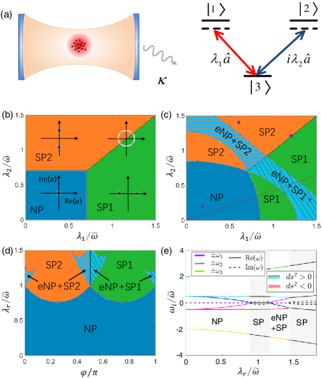
Figure 1: (a) Schematic illustration of the considered setup. An ensemble of V-typed three-level atoms are strongly coupled to a single-mode cavity field with dissipation rate $\kappa$. The cavity photons mediating the two atomic transitions are different by a phase rotation of $\pi/2$. (b-d) Phase diagrams of the nondissipative model showing NP (blue), SP1 (green), and SP2 (orange). The phase coexistence regions of e-NP and SP are represented by different colours with hatched patterns. The phase diagrams are plotted in the (b-c) $\lambda_{1}-\lambda_{2}$ plane and (d) $\varphi-\lambda_{r}$ plane with (b) $\varphi=\pi/4$, (c) $\varphi=7\pi/16$, and (d) $\lambda_{2}/\lambda_{1}=0.41$. Four distinct phases in (a) are indicated by their respective cavity-field distributions as a function of the real and imaginary parts of the cavity mode Re$\left\langle\hat{a}\right\rangle$ and Im$\left\langle\hat{a}\right\rangle$. (e) Real (solid) and imaginary (dashed) parts of the excitation energies $\pm\omega_{i}$ on top of the NP along the red dotted cut line in (c). The particlelike (holelike) fluctuations are denoted by blue, cyan, and green (magenta, red and yellow) lines, i.e., $ds^{2}>0$ ($ds^{2}<0$). The excitation spectra in the NP and e-NP are purely real whereas  some of their imaginary parts acquire a finite value in the SP (grey region). Note that crossing from the NP to the e-NP, the soft-mode excitations, $\pm\omega_{1}$, swap their sign of norms, indicating a particle-to-hole inversion. In these figures, $\lambda_{r}\equiv\sqrt{\lambda_{1}^{2}+\lambda_{2}^{2}}$, and $\omega=4\omega_{0}=2\tilde{\omega}$ with reference frequency $\tilde{\omega}\equiv\sqrt{\omega\omega_{0}}$.

II Model

We consider N identical V-type three-level atoms interacting with a single-mode cavity field. Each atom consists of one lowest level $\left|0\right\rangle$ and two degenerate levels $\left|1\right\rangle$ and $\left|2\right\rangle$ [see Fig. 1(a)]. The transitons $\left|0\right\rangle\longleftrightarrow\left|1\right\rangle$ and $\left|0\right\rangle\longleftrightarrow\left|2\right\rangle$ are mediated by cavity fields with phase difference of $\pi/2$, allowing potentially different co- and counter-rotating interactions. Such a scenario can be effectively engineered in atomic gases with long-lived hyperfine states. These states are then coupled by pump lasers and cavity field, which forms, typically unbalanced, Raman transitions (see Appendix A for descriptions of the proposed experimental configuration). The Hamiltonian describing this system reads

$$\hat{H} = \hbar\omega\hat{a}^{{\dagger}}\hat{a}+\hbar\omega_{0}\left(\hat{\Lambda}_{1,1}+\hat{\Lambda}_{2,2}\right)$$ (1)

$$+\left[\frac{\hbar\lambda_{1}}{\sqrt{N}}\hat{\Lambda}_{1,0}(\sin(\varphi)\hat{a}+\cos(\varphi)\hat{a}^{{\dagger}})\right.$$

$$\left.+\frac{i\hbar\lambda_{2}}{\sqrt{N}}\hat{\Lambda}_{2,0}(\sin(\varphi)\hat{a}-\cos(\varphi)\hat{a}^{{\dagger}})+\text{H.c.}\right],$$

where $\hat{a}$ is the annihilation operator of the cavity photon, $\hat{\Lambda}_{i,j}=\sum_{k=1}^{N}\left|i\right\rangle_{k}\left\langle j\right|_{k}$ ($i,j=1,2,3$) represent the collective spin operators, $\omega$ is the cavity frequency, $\omega_{0}$ denotes the transition frequency between level $\left|0\right\rangle$ and the two degenerate levels $\left|1\right\rangle$ and $\left|2\right\rangle$, and $\lambda_{\mu}$ ($\mu=1,2$) are the corresponding collective coupling strengths. Note that the parameter $\varphi$ is introduced to control the relative weight between the co- and counter-rotating terms. Observing the symmetry of the Hamiltonian under the transformations $\varphi\mapsto\varphi+\pi$ and $a\mapsto-a$, we can restrict the value range of $\varphi$ to $[0,\pi]$ without loss of generality. It follows that the corotating (counter-rotating) interaction overwhelms the counter-rotating (corotating) interaction for $\varphi\in(\pi/4,3\pi/4)$ ($\varphi\in[0,\pi/4)\cup(3\pi/4,\pi]$). The pseudospin operators $\Lambda_{i,j}$ can be mapped onto the Gell-Mann matrices, and thus spans the SU(3) symmetry space of Lie algebra book2 . This is in contrast to the pseudospin operators for the two-level Dicke model, which constitute the SU(2) commutation relation. This difference between the two atomic symmetries may lead to drastically different equation of motion and hence fundamentally influence the steady states ThreeDicke4 ; ThreeDicke5 ; ThreeDicke8 .

Hamiltonian (1) extends the standard two-level Dicke model to multiple distinct parameter regimes. For example, in the case of $\varphi=\pi/4$, the transitions between the atomic lowest level and the two excited levels are respectively coupled by two orthogonal quadratures of the cavity field, whose non-equilibrium features was considered in Refs. Dickelike9 ; ThreeDicke8 . While for $\lambda_{\mu}=0$ ($\mu=1,2$), the Hamiltonian (1) reduces to the interpolating Dicke-Tavis-Cummings model IDTC1 ; IDTC2 ; IDTC3 ; IDTC4 ; IDTC5 ; IDTC6 ; IDTC7 ; IDTC8 , which recovers the standard Dicke (Tavis-Cummings) model by further setting $\varphi=\pi/4$ ($\varphi=\pi/2$).

In general, the Hamiltonian (1) possess a double $\mathbb{Z}_{2}\otimes\mathbb{Z}_{2}$ symmetry, which is composed of the two other transformations $\left(\hat{a},\hat{\Lambda}_{10},\hat{\Lambda}_{20}\right)$ $\underrightarrow{\mathcal{T}_{1}}$ $\left(-\hat{a}^{{\dagger}},-\hat{\Lambda}_{01},\hat{\Lambda}_{02}\right)$ and $\left(\hat{a},\hat{\Lambda}_{10},\hat{\Lambda}_{20}\right)$ $\underrightarrow{\mathcal{T}_{2}}$ $\left(\hat{a}^{{\dagger}},\hat{\Lambda}_{01},-\hat{\Lambda}_{02}\right)$. This discrete symmetry can be enlarged to a U(1) symmetry in two specific cases: (i) $\varphi=n\pi/2$ ($n\in\mathbb{Z}$) and (ii) $\lambda_{1}=\lambda_{2}$. Depending on the parity of $n$, either the co-rotating or the counter-rotating term vanishes for case (i), leading to the U(1) symmetry found in the Tavis-Cummings (TC) model book0 ; TC . The U(1) symmetry in case (ii) is characterized by a nontrivial transformation $\hat{H}=$ $\hat{U}^{{\dagger}}(\vartheta)\hat{H}\hat{U}(\vartheta)$ with $\hat{U}(\vartheta)=\exp(i\vartheta\hat{G})$, and $\hat{G}=\hat{a}^{{\dagger}}\hat{a}+i(\hat{\Lambda}_{21}-\hat{\Lambda}_{12})$ satisfying $[\hat{H},\hat{G}]=0$. Notice that the conserved quantity $\hat{G}$ has also been pointed out in Refs. Dickelike9 ; ThreeDicke8 for the balcanced coupling case. We here show that the constraint on $\varphi(=\pi/4)$ can be completely relaxed, yielding a continuous family of models, each labeled by $\varphi$, that respect the same U(1) symmetry. In the spirit of Landau’s theory, the aforementioned symmetries of the Hamiltonian signals potential equilibrium or nonequilibrium phase transitions. In the following two sections, we provide a thorough analysis of the emergent quantum phases for both the nondissipative and dissipative models. For each model we first show the results of the balanced coupling case with $\varphi=\pi/4$, and then explore the effects of deviation from this balanced point.

III Phase diagram for the closed system

The static properties of a closed system is involved in its mean-field energy (ME) functional, which can be formally obtained by using an SU(3) generalization of the Holstein-Primakoff transformation (see Appendix B for details). A fluctuation analysis around the extrema of the ME determines the stability of various phases: the phase is physical and stable only if its fluctuation excitations acquire a completely real spectrum.

It is found that the NP, where the cavity mode is empty and the atoms populate the lowest level $\left|0\right\rangle$, is enclosed by the curve (Appendix C)

$$(2\left|\mathcal{B}\right|+L)^{2}-\omega^{2}\omega_{0}^{2}=0,$$ (2)

with $L=\lambda_{1}^{2}+\lambda_{2}^{2}$ and $\mathcal{B}=\cos(\varphi)\sin(\varphi)(\lambda_{1}^{2}-\lambda_{2}^{2})$. For parameters obeying $(2\left|\mathcal{B}\right|+L)^{2}>\omega^{2}\omega_{0}^{2}$, the system enters the SP by undergoing a second-order phase transition. In this phase, the cavity mode is macroscopically populated as $\left|\left\langle a\right\rangle\right|$ $=\sqrt{[(2\left|\mathcal{B}\right|+L)^{2}-\omega^{2}\omega_{0}^{2}]/4(2\left|\mathcal{B}\right|+L)\omega^{2}}$, and the atoms are partially excited to their higher energy levels $\left|1\right\rangle$ or $\left|2\right\rangle$. In the SP, the sign of $\mathcal{B}$ further distinguishes two distinct phases: for $\mathcal{B}>0$ ($\mathcal{B}<0$), the cavity mode acquires a real (imaginary) macroscopic excitation with Re$\left\langle\hat{a}\right\rangle\neq 0$ and Im$\left\langle\hat{a}\right\rangle=0$ (Re$\left\langle\hat{a}\right\rangle=0$ and Im$\left\langle\hat{a}\right\rangle\neq 0$), and the $\mathcal{T}_{1}$ ($\mathcal{T}_{2}$) symmetry is spontaneously broken. We term the SP with $\mathcal{B}>0$ superradiant phase 1 (SP1), and that with $\mathcal{B}<0$ superradiant phase 2 (SP2). The critical curve $\mathcal{B}=0$, along which the Hamlitonian respects a U(1) symmetry, determines a first order phase boundary between the SP1 and SP2.

A typical parameters choice is the balanced driving case with $\varphi=\pi/4$. In this case, the counter-rotating and corotating interactions feature on an equal footing. The closed phase diagram is outlined in Fig. 1(b). For $\lambda_{1},\lambda_{2}\leqslant$ $\lambda_{c}\equiv\sqrt{\omega\omega_{0}/2}$, the system is located in the NP. Tunning one of the coupling strength above the critical value $\lambda_{c}$, namely$\ \max(\lambda_{1}$,$\lambda_{2})>\lambda_{c}$, the system enters the SP. The U(1)-symmetry line $\lambda_{1}=\lambda_{2}>\lambda_{c}$ splits the SP into two subphases: the SP1 with $\lambda_{1}>\lambda_{2}$ and the SP2 with $\lambda_{2}>\lambda_{1}$.

Allowing the coupling strength of the counter-rotating and corotating terms unbalanced, say $\varphi\neq\pi/4$, results in richer phenomena. The phase diagram of $\varphi=7\pi/16$ is representatively plotted in Fig. 1(c). Different from the balanced case [Fig. 1(b)], deep inside the SP, a considerably large region where NP is also stable, emerges. We remark that this NP is essentially a stable exited state since it corresponds to a local maximum of the ME landscape (see Appendix C for detailed description). Following the nomenclature used in Ref. IDTC6 , we hereafter dub the NP, which coexists with the SP, exited-Normal phase (e-NP). To see the impacts of the unbalanced co- and counter-rotating interactions more clearly, we plot in Fig. 1(d) the phase diagram as a function of $\varphi$ and the coupling strength $\lambda_{r}\equiv\sqrt{\lambda_{1}^{2}+\lambda_{2}^{2}}$ with $\lambda_{2}/\lambda_{1}=0.41$. It is to be seen that, as the system deviates away from the balanced point $\varphi=\pi/4$, the regions of the phase coexistence of SP and e-NP becomes pronounced.

Apart from the ME landscape, the NP and e-NP are dynamically distinct by the nature of excitations: at positive (negative) eigenfrequencies, the soft-mode excitations of both NP and SP are particlelike (holelike), whereas those of e-NP are holelike (particlelike) IDTC6 ; IDTC7 . This can be confirmed by investigating the sympletic norm, $ds_{\mathbf{v}_{j}}^{2}\equiv$ $\mathbf{v}_{j}^{{\dagger}}I_{z}\mathbf{v}_{j}$, defined at each normal-mode eigenfrequency, where $\mathbf{v}_{j}$ with $j=1,...,2N$ are the eigenvectors of the Hopfeld-Bogoliubov matrix $D_{\text{H}}$ (see Appendix C), and $I_{z}=1_{N}\otimes(-1_{N})$  is a $2N\times$ $2N$ diagonal matrix with $+1$ ($-1$) entries on the first (second) $N$ elements. The nature of the excitations is intimately related to the sign of $ds_{\mathbf{v}_{j}}^{2}$. That is, the soft mode is a particlelike (holelike) excitation at positive eigenfrequencies for $ds_{\mathbf{v}_{j}}^{2}>0$ ($ds_{\mathbf{v}_{j}}^{2}<0$), and is a holelike (particlelike) excitation at negative eigenfrequencies for $ds_{\mathbf{v}_{j}}^{2}<0$ ($ds_{\mathbf{v}_{j}}^{2}>0$). Figure 1(e) depicts the excitation spectra and the sign of their sympletic norms on top of the NP along a representative trajectory in parameter space [cf. Fig 1(c)]. As the coupling strength increases, the system traverses NP, SP, coexistence of e-NP and SP, and eventually end in SP. While, as expected, the whole spectra are purely real in the NP and e-NP, the soft-mode pair, $\pm\omega_{1}$, swap their sign of sympletic norms, indicating a particle-to-hole inversion.

IV Steady state in the presence of cavity dissipation

The above picture fundamentally changes if the dissipative nature is explicitly considered. To provide an understanding of the open phase diagram, we start from the master equation of the form $\partial_{t}\hat{\rho}=\mathcal{\hat{L}}\hat{\rho}$, where the Liouvillian acts as $\mathcal{\hat{L}}\hat{\rho}=-i/\hbar[\hat{H},\hat{\rho}]+\kappa(2\hat{a}\hat{\rho}\hat{a}^{{\dagger}}-\hat{a}^{{\dagger}}\hat{a}\hat{\rho}-\hat{\rho}\hat{a}^{{\dagger}}\hat{a})$ with $\kappa$ being the photon loss rate. The steady-state properties of the open system are captured by a stability analysis of the Liouvillian’s fixed points, which can be effectively achieved under the framework of third quantization ThirdQuant1 ; ThirdQuant2 . This approach produces a set of rapidities {$\zeta_{i}$}, whose role resembles that of the excitation spectrum of closed systems: the real and imaginary parts of $\zeta_{i}$ characterizes the lifetime and frequency of the corresponding fluctuation mode, respectively. The steady state is stable when the real parts of all the rapidities are nonnegative, i.e., Re$\zeta_{i}\geqslant 0$. The detailed calculations of {$\zeta_{i}$} is attributed to the Appendix D. In principle, the stable attractors of the open system can either lie in the low energy sectors with most of the atoms populating the lowest energy level $\left|0\right\rangle$, or the high energy sectors where the atomic population are completely inverted to the exited states $\left|1\right\rangle$ and $\left|2\right\rangle$. The superradiant features can only be highlighted in the low energy sectors, which is the focus of this Section. We leave the discussion of relevant physics in the high energy sectors in Sec. V.

A generic impact of the cavity dissipation imposed on the system is the elimination of the U(1)-symmetry-broken phase IDTC3 ; Dickelike2 ; Dickelike3 ; Dickelike4 ; Dickelike9 ; ThreeDicke8 along the critical curve $\mathcal{B}=0$. The SP, which features both populated real and imaginary quadratures of the cavity mode in the open case (i.e., Re$\left\langle\hat{a}\right\rangle\cdot$Im$\left\langle\hat{a}\right\rangle\neq 0$), is stable inside multiple disconnected phase regions separated by $\mathcal{B}=0$. As shown in Fig. 2(c), the open phase diagram of $\varphi=\pi/4$ is sharply different from its closed counterpart [cf. Fig. 1(b)] in the following aspects: Dickelike9 (i) the NP is generically destabilized in the parameter space, except for the two-level limit $\lambda_{\mu}=0$ ($\mu=1,2$), (ii) the SP along a $\kappa$-dependent sliver around the U(1) symmetry line $\lambda_{1}=\lambda_{2}$, vanishes, and (iii) the continuous phase boundary enclosing the superradiant region with $\lambda_{1}\cdot\lambda_{2}\neq 0$, becomes first order.

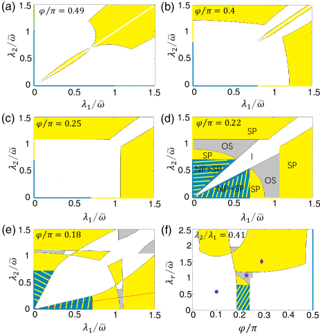
Figure 2: Steady-state phase diagrams of the dissipative model showing NP (blue), SP (yellow), OS (grey) and coexistence of NP and SP (hatched yellow and blue) with $\omega=4\omega_{0}=2\tilde{\omega}$ and $\kappa=0.1\tilde{\omega}$. Note that, except for the two limits $\lambda_{1}\cdot\lambda_{2}=0$ and $\varphi=(n+1)\pi/2$ ($n\in\mathbb{Z}$), the inverted states are stable throughout the whole parameter space. They are either the exclusive steady states (white) or coexistent with other phases (indicated by colours other than white). (a-e) Evolution of the phase diagram in $(\lambda_{1}$, $\lambda_{2})$ plane as one varies $\varphi$ from the co-rotating side $\varphi/\pi=0.49$ to the counter-rotating side $\varphi/\pi=0.18$. (f) $\lambda_{r}$ vs $\varphi$ for fixed $\lambda_{2}/\lambda_{1}=0.41$.

The phase diagram exhibits distinctly different features in the co- and counter-rotating-dominated regimes. We first pay attention to the corotating side with $\varphi\in(\pi/4,\pi/2]$ remark . For corotating coupling strength slightly larger than the counter-rotating one, two small islands of SP, splitted by the U(1) line $\lambda_{1}=\lambda_{2}$, emerg inside the $\kappa$-dependent sliver [Fig. 2(b)]. As $\varphi$ increases further, the area of the two SP islands enlarges and even percolates to parameter space with extremely small coupling strength $\lambda_{\mu}$ ($\mu=1,2$), and the $\kappa$-dependent sliver which prevents the superradiance transition is eventually destroyed [Fig. 2(a)].

The physics in the counter-rotating-dominated side with $\varphi\in[0,\pi/4)$ is richer. The first finding is the appearance of steady-state solutions converging to limit cycles instead of fixed points, as denoted in Figs. 2(d)-(f). The limit cycles dictate an oscillatory supperradiant phase (OS) in which the order parameters exhibit persistent oscillation around some nonzero values. Figure 3(a) shows the dynamical evolutions of the order parameters in three different parameter regimes. While the steady state belonging to SP is time independent [middle panel of Fig. 3(a)], the stable oscillatory character of dynamical variables in the OS is clearly identified after a sufficiently long integration time [bottom panel of Fig. 3(a)]. We remark that the regimes of persistent oscillations also exist in the open SU(2) Dicke model with unbalanced coupling IDTC5 ; IDTCexp1 . It is also found that the NP, which is generically destabilized in the balanced coupling case, stably coexists with the SP in a pie-chart-shaped region in $\lambda_{1}-\lambda_{2}$ plane [Figs. 2(d)-(e)]. In this multi-phase coexistence region, the SP solution looks a bit counter-intuitive as it decreases to zero as the coupling strength increases [see Fig. 3(b) for illustration]. This is in sharp contrast to the standard Dicke model Dicke2 , where a monotonic increasing behavior of the order parameters is observed. The critical value of the coupling strength, at which the order parameters of the SP vanish, defines a second-order phase boundary. We emphasize that, except for the continuous phase boundary appeared here and those for the two-level limit $\lambda_{\mu}=0$ ($\mu=1,2$), all the other steady-state phase transitions with $\kappa\neq 0$ are of first order. In $\lambda_{1}-\lambda_{2}$ plane, the area of NP-SP coexisting phase reduces as the system approaches the counter-rotating-dominated side, until it vanishes at a critical value $\varphi_{c}$. The existence of such criticality becomes immediately clearer if we plot the phase diagram as a function of $\varphi$ and $\lambda_{r}$ for fixed $\lambda_{1}/\lambda_{2}$ [Fig. 2(f)]. As another interesting aspects demonstrated by this figure, while the NP keeps stable with $\varphi=\pi/2$, an infinitely small counter-rotating fraction may destabilize it and drive the fixed points to a family of inverted states in the high energy sectors [represented by the white region in Fig. 2(f)]. The counter-rotating terms represent a process explicitly breaking the energy conservation, which is commonly believed of less significance for weak enough coupling strength book . Our results here show that these terms, although vanishingly small, deserves special attention when the atomic symmetry is enlarged. An in-depth investigation of this subject is out of the scope of this paper and will be attributed to future work.

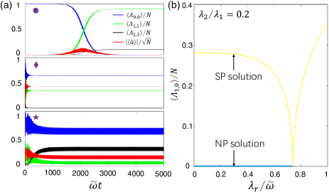
Figure 3: (a) Dynamical evolutions of the cavity field amplitude and atomic populations for the corresponding parameter locations indicated by the symbols of round, diamond, and star in Fig. 2 (f). In this simulation, the initial state is chosen as the normal state ($\left\langle\hat{\Lambda}_{0,0}\right\rangle=N$, $\left\langle\hat{\Lambda}_{0,j}\right\rangle=\left\langle\hat{\Lambda}_{i,j}\right\rangle$ for $i,j\in\{1,2\}$) with a small cavity field $\left\langle\hat{a}\right\rangle/\sqrt{N}=0.01$ (see Appendix E for the equations of motion). (b) The stable steady-state solutions of the atomic field $\left\langle\hat{\Lambda}_{0,1}\right\rangle$ as a function of $\lambda_{r}$ for fixed $\varphi=0.18\pi$ and $\lambda_{2}/\lambda_{1}=0.2$, i.e., along the red dotted cut line in Fig. 2(e).

V Dissipation stabilized Inverted state

Up to now, the quantum states we discussed are restricted to the low energy sectors where the atomic lowest level $\left|0\right\rangle$ is macroscopically populated. There is, however, a different class of states with unoccupied $\left|0\right\rangle$. These inverted states, having a much higher energy than those of the NP and SP, are characterized by two parameters

$$N_{1}=\left\langle\hat{\Lambda}_{11}\right\rangle\text{, and }\theta=\arg\left\langle\hat{\Lambda}_{12}\right\rangle$$ (3)

which respectively denotes the occupation of level $\left|1\right\rangle$ and the relative phase between levels $\left|1\right\rangle$ and $\left|2\right\rangle$. The collective states determined by parameters (3) are essentially spin coherent state in the inverted-state subspace. Of particular importance in the class of inverted spin coherent states is the dark state defined as Dark1 ; Dark2

$$\left|D\right\rangle=\prod_{j=1}^{N}\left|d\right\rangle_{j},$$ (4)

where $\left|d\right\rangle=$ $i\sin(\nu)\left|1\right\rangle+\cos(\nu)\left|2\right\rangle$ and $\tan(\nu)=\lambda_{2}/\lambda_{1}$. Note that with this definition, the state $\left|D\right\rangle$ is uniquely defined by the parameter $\nu$. The dark state (4) is completely decoupled from the radiation field and therefore becomes a stable eigenstate of the Hamiltonian (1). The lack of adiabatic passage makes the inverted states less important in the closed system. They, nevertheless, become crucial under the open environment due to their accessibility provided by the cavity dissipation IDTC1 ; IDTC2 ; IDTC6 ; IDTC7 .

It should be noticed that, while all the inverted spin coherent states turn out to be fixed points of the Liouvillian $\mathcal{\hat{L}}$, only a subset of them is stable. By analyzing the related rapidities, it is found that the stable fixed points fall into a region enclosed by a stability boundary in the $\theta-N_{1}$ plane,

$$\frac{2\eta_{1}\eta_{2}\sin(\theta)}{\eta_{1}^{2}+\eta_{2}^{2}}=\frac{(\kappa^{2}+\omega^{2}+\omega_{0}^{2})\cos(2\varphi)-2\omega_{0}\omega}{\kappa^{2}+\omega^{2}+\omega_{0}^{2}-2\omega_{0}\omega\cos(2\varphi)}\equiv\Omega$$ (5)

where $\eta_{1}=$ $\lambda_{1}N_{1}/\sqrt{N}$ and $\eta_{2}=\lambda_{2}\sqrt{1-N_{1}/N}$, and the role of the parameter $\varphi$ is encapsulated in the scaled variable $\Omega$. Setting $\varphi=\pi/4$, we reproduce the result of the balanced case obtained in Ref. ThreeDicke8 , in which the value of $\Omega$ are restricted in between $0$ and $1$ by definition. Allowing the parameter $\varphi$ tunable, however, feasible range of the scaled variable $\Omega$ is extended to $[-1,1]$. As is detailed in the following, the enlargement of the value range of $\Omega$ provides new possibilities to engineer the atomic steady state.

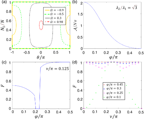
Figure 4: (a) Stability boundaries of the inverted state in the $\theta-N_{1}$ parameters space for $\lambda_{1}=\lambda_{2}$ and different $\Omega$. Solutions inside the regions enclosed are stable. Note that here the parameter $\theta$ is shifted by $\pi/2$ for clarity. (b) Evolution of the area $\mathcal{A}$ as a function of $\varphi$ for $\lambda_{2}/\lambda_{1}=\sqrt{3}$ and $\kappa=0.1\tilde{\omega}$. (c-d) Fidelities given by Eq. (7) for $\kappa=\tilde{\omega}$ as a function of (c) $\varphi$ with $\nu=\pi/8$, and (d) $\nu$ with varying $\varphi$. The density matrix $\rho_{s}$ is obtained by  integrating the mean-field equations of motion until a steady state can be identified. The other parameters are $\omega=4\omega_{0}=2\tilde{\omega}$.

With the stability boundary defined in Eq. (5), the area of the enclosed region is derived as $\mathcal{A}=$ $N\pi[1-\Omega(\lambda_{1}^{2}+\lambda_{2}^{2})/\sqrt{\Omega^{2}(\lambda_{1}^{2}-\lambda_{2}^{2})^{2}+4\lambda_{1}^{2}\lambda_{2}^{2}}]$ ThreeDicke8 . We plot the the stability boundary Eq. (5) for several representative parameters in Fig. 4(a). The trend that $\mathcal{A}$ increases with the decrease of $\Omega$ is obvious. More importantly, tuning the model from the corotating side to the counter-rotating side by varying $\varphi$, $\Omega$ goes from $1$ to $-1$, and the area of the stable region increases from $0$ to $2\pi N$, as is illustrated in Fig. 4(b).

The two end points, $\varphi=0$ and $\varphi=\pi/2$, deserve special attention, since the values of $\mathcal{A}$ in these two cases are best understandable through a purely physical argument. The multistability for a more general value $\varphi\in(0,\pi/2)$ interpolate between the two limit cases. Let us focus on $\varphi=\pi/2$ first. In this case, the Hamiltonian (1) is simplified to a three-level TC-like model,

$$\hat{H}=\hat{H}_{TC}+\omega_{0}\hat{\Lambda}_{d,d},$$ (6)

where $\hat{H}_{TC}=$ $\hbar\omega\hat{a}^{{\dagger}}\hat{a}+\omega_{0}\hat{\Lambda}_{r,r}+\hbar\lambda_{r}(\hat{\Lambda}_{r,0}a+\hat{\Lambda}_{0,r}a^{{\dagger}})$ is the TC Hamiltonian with $\left|r\right\rangle=\cos(\nu)\left|1\right\rangle+i\sin(\nu)\left|2\right\rangle$ being a single-particle bright state. Since the open TC model stablizes only the NP IDTC3 , the dark state $\left|D\right\rangle$ becomes the only stable inverted state, manifesting a single point in the $\theta-N_{1}$ parameters space (i.e., $\mathcal{A}=0$). We then turn to the other limit $\varphi=0$, where the light-matter interaction is purely governed by the counter-rotating terms. In this regime, the variation of the excitation number for both spin and bosonic parts is one, whereas that for the light-matter polariton mode is two. It is straightforward to show that this scheme prohibits the direct transition between the atomic inverted states with vacuum photon mode and any other states in the Hilbert space. Hence, atoms in the inverted-state subspace are all decoupled from the radiation field, meaning that the stable region occupies the whole $\theta-N_{1}$ parameters space.

The preparation of a spin coherent state with required population projection on the levels $\left|1\right\rangle$ and $\left|2\right\rangle$ is always one of the central aims in the atomic physics. The fact that our model hosts a single stable inverted state $\left|D\right\rangle$ in the TC limit $\varphi=\pi/2$, for which the population projection is tuned by the system parameter $\nu$, suggests a potential scenario to achieve this goal. However, in this case, a general initial state will not evolve to the state $\left|D\right\rangle$ due to its darkness, but instead dissipates to the lowest level $\left|0\right\rangle$ CRT0 . Fortunately, as is illustrated in Sec. IV, even an infinitely small counter-rotating coupling can destabilize the level $\left|0\right\rangle$ and drives the fixed points to a multistable region of inverted states, which are bounded by a closed curve in the $\theta-N_{1}$ plane. Considering the region of multistability shrinks to the representative point of $\left|D\right\rangle$ as the counter-rotating coupling strength decreases to zero, a natural anticipation is, from a general initial state, the steady state can approache the dark state $\left|D\right\rangle$ in a similar fashion. To verify this, we can look at the fidelity of the steady state Fidelity1 ; Fidelity2 ,

$$F=Tr\left(\hat{\rho}_{s}\hat{\rho}_{d}\right)$$ (7)

where $\hat{\rho}_{d}$ and $\hat{\rho}_{s}$ denote the density operators of the dark state $\left|D\right\rangle$, which can be the target state in demand, and the steady state of the master equation $\partial_{t}\hat{\rho}=\mathcal{\hat{L}}\hat{\rho}$, respectively. The fidelity Eq. (7) quantifies the similarity between $\hat{\rho}_{s}$ and $\hat{\rho}_{d}$, and it turns out to be 1 if $\hat{\rho}_{s}=\hat{\rho}_{d}$, otherwise $0\leqslant F<1$. Figure. 4(c) depicts the fidelity $F$ as a function of $\varphi$ for fixed $\lambda_{1}$, $\lambda_{2}$ and $\kappa$. As expected, in the co-rotating dominated regime, the fidelity increases and finally approaches identity as $\varphi$ gets close to $\pi/2$. Note that $F$ touches zero in an intermediate region, due to the stabilization of the NP by the counter-rotating interaction [cf. Fig. 2(f)]. To demonstrate the feasibility of preparing a steady state with arbitrary population projection on the levels $\left|1\right\rangle$ and $\left|2\right\rangle$, we plot $F$ as a function of $\nu$ for varying $\varphi$ in Fig. 4(d). It can be seen clearly that, tuning $\varphi$ to the co-rotating-dominated side, $F$ gets closed to some constant for all values of $\nu\in(0,\pi/2)$, despite of small fluctuations. More importantly, the closer to the co-rotating side, the higher the fidelity is.

Before ending this section, we make two remarks. Firstly, the above predictions for the fidelity depend crucially on the SU(3) atomic symmetry. The vanishing of either the coupling strength $\lambda_{1}$ or $\lambda_{2}$ reduces the atomic symmetry to SU(2), and thus essentially changes the system dynamics. This explains the two exceptions occurring for $\nu=0$ and $\pi/2$ in Fig. 4(d), where $F$ drops to zero. Secondly, the proposed approach of state preparation can make the population projections on levels $\left|1\right\rangle$ and $\left|2\right\rangle$ controllable, but leaves the relative phase between them fixed. The engineering of an inverted steady state with arbitrary relative phase can be achieved by encoding a tunable phase-difference rotation between the cavity photons which mediate the two atomic transitions $\left|0\right\rangle\longleftrightarrow\left|1\right\rangle$ and $\left|0\right\rangle\longleftrightarrow\left|2\right\rangle$. An in-depth investigation of this scenario, albeit at the cost of added complexity, merits a separate work.

VI Conclusions

We have investigated a system of V-typed three-level atoms interacting with a single-mode cavity field, with main focus on the consequences of the competition between the co- and counter-rotating interaction. Using a mean-field approach and third quantization analysis, we have mapped out the phase diagram of the system for both closed and open conditions. Rich quantum phase behaviours, including multi-phase coexistence and limit cycle oscillation, has been revealed. Of particular interesting is the inverted spin coherent steady states stabilized by the cavity dissipation. By analyzing the roles of the co- and counter-rotating terms in the inverted-state stabilization, we have proposed a high-fidelity state preparation scenario.

Appendix A Effective Hamiltonian and proposed experimental implementation

In this Section, we propose an experimental implementation of our model based on distinct cavity-assisted Raman transitions of cold atoms DickeP . As shown in Fig. 5(a), an ensemble of ⁸⁷Rb atoms is trapped within an optical cavity by an intracavity optical lattice IDTCexp1 ; IDTCexp2 . The atoms are driven transverse to the cavity by two pairs of lasers. Each pair of the lasers is composed of two counter-propagating single beams with different circular polarization. A guided magnetic field $B$ is applied along the direction of the laser propagation ($z$ direction) to fix a quantized axis and split the Zeeman sublevels of the atomic ensemble, which confirms the distinct Raman channels. The cavity field is linearly polarized along the $y$ axis, which is perpendicular to the magnetic field. The three hyperfine sublevels of 5$S_{1/2}$, $\left|F=2,m_{F}=+2\right\rangle$, $\left|F=1,m_{F}=0\right\rangle$, and $\left|F=2,m_{F}=-2\right\rangle$, can play the roles of atomic levels $\left|1\right\rangle,$ $\left|0\right\rangle,$ and $\left|2\right\rangle$, respectively. The two pairs of counter-propagating lasers, with Rabi frequencies (phases) $\Omega_{s_{1,2}}$ and $\Omega_{r_{1,2}}$ ($\theta_{s_{1,2}}$ and $\theta_{r_{1,2}}$), provide optical couplings between 5$S_{1/2}$ and 5$P_{3/2}$, and thus form four distinct Raman transitions, as shown in Fig. 5(b). The detunnings of driving lasers from the excited states, $\Delta_{s_{1,2}}$ and $\Delta_{r_{1,2}}$, are assumed large enough so that we can adiabatically eliminate the 5$P_{3/2}$ levels, yielding an effective Hamiltonian

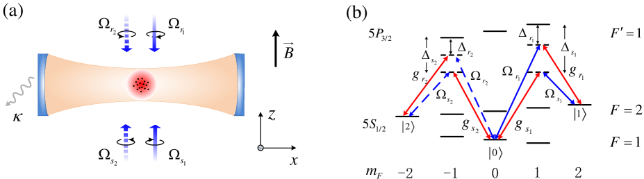
Figure 5: (a)The proposed experimental setup and (b) possible atomic excitation scheme based on the $D_{2}$ line of ⁸⁷Rb atom.

$$\hat{H} = \omega_{A}\hat{a}^{\dagger}\hat{a}+\sum_{j=1}^{N}\left(\omega_{00}\left|0\right\rangle_{j}\left\langle 0\right|_{j}+\omega_{10}\left|1\right\rangle_{j}\left\langle 1\right|_{j}+\omega_{20}\left|2\right\rangle_{j}\left\langle 2\right|_{j}\right)$$ (8)

$$+\hat{a}^{\dagger}\hat{a}\sum_{j=1}^{N}\left[g_{r}(\mathbf{r}_{j})\left(\frac{\left|1\right\rangle_{j}\left\langle 1\right|_{j}}{\Delta_{r_{1}}}+\frac{\left|2\right\rangle_{j}\left\langle 2\right|_{j}}{\Delta_{r_{2}}}\right)+g_{s}(\mathbf{r}_{j})\left|0\right\rangle_{j}\left\langle 0\right|_{j}\left(\frac{1}{\Delta_{s_{1}}}+\frac{1}{\Delta_{s_{2}}}\right)\right]$$

$$+\sum_{\tau=1}^{2}\sum_{j=1}^{N}\left[\frac{\Omega_{s_{\tau}}g_{s}(\mathbf{r}_{j})}{2\Delta_{s_{\tau}}}\hat{a}\left|\tau\right\rangle_{j}\left\langle 0\right|_{j}e^{-i(\mathbf{k}_{s_{\tau}}\cdot\mathbf{r}_{j}+\theta_{s_{\tau}})}+\frac{\Omega_{r_{\tau}}g_{r}(\mathbf{r}_{j})}{2\Delta_{r_{\tau}}}\hat{a}\left|0\right\rangle_{j}\left\langle\tau\right|_{j}e^{-i(\mathbf{k}_{r_{\tau}}\cdot\mathbf{r}_{j}+\theta_{r_{\tau}})}+\text{H.c.}\right]$$

where the definitions

$$\left|1\right\rangle\equiv\left|F=2,m_{F}=+2\right\rangle,$$ (9)

$$\left|0\right\rangle\equiv\left|F=1,m_{F}=0\right\rangle,$$ (10)

and

$$\left|2\right\rangle\equiv\left|F=2,m_{F}=-2\right\rangle$$ (11)

has been made. In the Hamiltonian (8), $g_{s}(\mathbf{r}_{j})$ [$g_{r}(\mathbf{r}_{j})$] is the single-photon coupling strength at position $\mathbf{r}_{j}$ mediating the transitions $\left|0\right\rangle\longleftrightarrow\left|F^{\prime}=1,m_{F^{\prime}}=+1\right\rangle$ and $\left|0\right\rangle\longleftrightarrow\left|F^{\prime}=1,m_{F^{\prime}}=-1\right\rangle$ ($\left|2\right\rangle\longleftrightarrow\left|F^{\prime}=1,m_{F^{\prime}}=-1\right\rangle$ and $\left|1\right\rangle\longleftrightarrow\left|F^{\prime}=1,m_{F^{\prime}}=+1\right\rangle$), and the model paremeters $\omega_{A}$, $\omega_{00}$, $\omega_{10}$, and $\omega_{20}$ are given by

$$\omega_{A}=\omega_{c}-\frac{\omega_{r_{1}}+\omega_{s_{1}}}{2}$$ (12)

$$\omega_{00}=\Omega_{r_{1}}^{2}/4\Delta_{r_{1}}+\Omega_{r_{2}}^{2}/4\Delta_{r_{2}}$$ (13)

$$\omega_{10}=\omega_{G_{1}}+\Omega_{s_{1}}^{2}/4\Delta_{s_{1}}-\frac{\omega_{r_{1}}-\omega_{s_{1}}}{2}$$ (14)

$$\omega_{20}=\omega_{G_{2}}+\Omega_{s_{2}}^{2}/4\Delta_{s_{2}}-\frac{\omega_{r_{2}}-\omega_{s_{2}}}{2}$$ (15)

where $\omega_{r_{1,2}}$ and $\omega_{s_{1,2}}$ are the frequencies of the driving lasers, $\omega_{G_{1}}$ ($\omega_{G_{2}}$) characterizes the energy of atomic level $\left|1\right\rangle$ ($\left|2\right\rangle$), and $\omega_{c}$ denotes the cavity frequency. We further assume the atoms are trapped to antinodes of the cavity field, so that the single-photon coupling strengths can be approximately constant and written in a position-independent form $g_{r/s}(\mathbf{r}_{j})=g_{r/s}$. For cold atoms with temperature closed to zero, the motional effect can be neglected meaning that the atom positions can be treated as classical variables DickeTheory1 ; IDTCexp2 . Bearing these assumptions in mind, and applying the unitary transformation

$$U_{\mathbf{k}}=\prod_{j=1}^{N}\exp\left[i(\mathbf{k\cdot r}_{j}+\frac{\theta_{r_{1}}+\theta_{r_{2}}-\theta_{s_{1}}-\theta_{s_{2}}}{2})(\left|1\right\rangle_{j}\left\langle 1\right|_{j}+\left|2\right\rangle_{j}\left\langle 2\right|_{j})-i\frac{\theta_{r_{1}}+\theta_{s_{1}}}{2}\hat{a}^{\dagger}\hat{a}\right],$$ (16)

the Hamiltonian (8) becomes

$$H = \omega_{A}\hat{a}^{\dagger}\hat{a}+\omega_{00}\hat{\Lambda}_{0,0}+\omega_{10}\hat{\Lambda}_{1,1}+\omega_{20}\hat{\Lambda}_{2,2}$$ (17)

$$+a^{\dagger}a\left[\hat{\Lambda}_{1,1}\frac{g_{r}}{\Delta_{r_{1}}}+\hat{\Lambda}_{2,2}\frac{g_{r}}{\Delta_{r_{2}}}+\hat{\Lambda}_{0,0}\left(\frac{g_{s}}{\Delta_{s_{1}}}+\frac{g_{s}}{\Delta_{s_{2}}}\right)\right]$$

$$+\left[\frac{\Omega_{s_{1}}g_{s}}{2\Delta_{s_{1}}}\hat{a}\hat{\Lambda}_{1,0}+\frac{\Omega_{r_{1}}g_{r}}{2\Delta_{r_{1}}}\hat{a}\hat{\Lambda}_{0,1}+\frac{\Omega_{s_{2}}g_{s}}{2\Delta_{s_{2}}}\hat{a}\hat{\Lambda}_{2,0}e^{i\tilde{\theta}}\right.$$

$$\left.+\frac{\Omega_{r_{2}}g_{r}}{2\Delta_{r_{2}}}\hat{a}\hat{\Lambda}_{0,2}e^{i\tilde{\theta}}+\text{H.c.}\right]$$

where $\tilde{\theta}=(\theta_{r_{1}}+\theta_{s_{1}}-\theta_{r_{2}}-\theta_{s_{2}})/2$ and the relation $\mathbf{k}_{r}\approx-\mathbf{k}_{s}=\mathbf{k}$ has been used.

When the parameters are chosen as $g_{r}/\Delta_{r_{1}}=g_{r}/\Delta_{r_{2}}=g_{s}/\Delta_{s_{1}}+g_{s}/\Delta_{s_{2}}$ and $\tilde{\theta}=\pi/2$, the Hamiltonian (17) reduces to

$$H = \hbar\omega\hat{a}^{{\dagger}}\hat{a}+\hbar\omega_{10}\hat{\Lambda}_{1,1}+\hbar\omega_{20}\hat{\Lambda}_{2,2}$$ (18)

$$+\left[\frac{\hbar\lambda_{1,s}}{\sqrt{N}}\hat{a}\hat{\Lambda}_{1,0}+\frac{\hbar\lambda_{1,r}}{\sqrt{N}}\hat{a}\hat{\Lambda}_{0,1}+i\frac{\hbar\lambda_{2,s}}{\sqrt{N}}\hat{a}\hat{\Lambda}_{2,0}\right.$$

$$\left.+i\frac{\hbar\lambda_{2,r}}{\sqrt{N}}\hat{a}\hat{\Lambda}_{0,2}+\text{H.c.}\right]$$

where

$$\omega=\omega_{A}+\frac{3Ng_{r}}{\Delta_{r_{1}}}$$ (19)

$$\lambda_{\tau,s}=\frac{\sqrt{N}\Omega_{s_{\tau}}g_{s}}{2\Delta_{s_{\tau}}}\text{ \ (}\tau=1,2\text{)}$$ (20)

and

$$\lambda_{\tau,r}=\frac{\sqrt{N}\Omega_{r_{\tau}}g_{r}}{2\Delta_{r_{\tau}}}\text{ \ (}\tau=1,2\text{)}$$ (21)

By requiring $\omega_{10}=$ $\omega_{20}=\omega_{0}$ and reparametrizing the collective coupling strength as

$$\lambda_{\tau,s}=\sin(\varphi)\lambda_{\tau}\text{, }\lambda_{\tau,r}=\cos(\varphi)\lambda_{\tau}\text{ \ \ (}\tau=1,2\text{),}$$ (22)

Eq. (18) reduces to Hamiltonian (1) in the main text.

Based on the energy levels and their transitions of ⁸⁷Rb atoms RbTab , together with the current experimental conditions IDTCexp1 ; IDTCexp2 , the atom-photon coupling strength can reach $g_{r}/2\pi=0.25$ MHz and $g_{s}/2\pi=0.14$ MHz, respectively. The number of trapped atoms, typically $N$ $\char 126\relax$ 10⁶ IDTCexp2 , appears to be practical. The atomic detunnings $\Delta_{s_{1,2}}$ and $\Delta_{r_{1,2}}$ can range from $1$ to $100$ GHz, and the parameters ($\left|\Omega_{r_{1,2}}\right|,\left|\Omega_{s_{1,2}}\right|,\kappa$) are on the order of a few megahertz. Therefore, the condition for the adiabatic elimination of the atomic levels, ($\left|\Delta_{s_{1,2}}\right|,\left|\Delta_{r_{1,2}}\right|$) $\gg$ ($\left|\Omega_{r_{1,2}}\right|,\left|\Omega_{s_{1,2}}\right|,g_{r},g_{s}$), is well satisfied. With these parameter setting, the collective coupling strength $\lambda_{1}$ and $\lambda_{2}$ can be tuned from zero to the order of megahertz, making the superradiant condition $\lambda_{1}(\lambda_{2})\geqslant\lambda_{c}$ achievable.

Appendix B Holstein-Primakoff transformation and the fluctuation Hamiltonian

In this Section, we derive the effective Hamiltonians describing fluctuations around various quantum states. These fluctuation Hamiltonians are necessary in analyzing the stability of considered states, and can be formally obtained using a generalized Holstein-Primakoff transformation HPP1 ; HPP2 . For system with three atomic levels, the Holstein-Primakoff transformation is implemented by rewriting the atomic operators $\hat{\Lambda}_{i,j}$ as

$$\hat{\Lambda}_{m,m} = N-\sum_{j\neq m}\hat{b}_{j}^{{\dagger}}\hat{b}_{j}\text{, }\hat{\Lambda}_{sk}=\hat{b}_{s}^{{\dagger}}\hat{b}_{k}\text{ (}s,k\neq m\text{)},\text{ }$$ (23)

$$\hat{\Lambda}_{s,m} = \hat{b}_{s}^{{\dagger}}\sqrt{N-\sum_{j\neq m}\hat{b}_{j}^{{\dagger}}\hat{b}_{j}}$$

where $\hat{b}_{j}^{{\dagger}}$ and $\hat{b}_{j}$ are bosonic creation and annihilation operators, respectively. In Eq. (23), the subscript $m$ labels a reference state around which the fluctuations are considered. We choose $\left|m\right\rangle=\left|0\right\rangle$ for the normal and superradiant states, and $\left|m\right\rangle=\left|1\right\rangle$ for the inverted state. Employing the transformations Eq. (23) and choosing appropriate reference states, the Hamiltonian (1) can be rewritten as

$$\hat{H} = \hbar\omega\hat{a}^{{\dagger}}\hat{a}+\hbar\omega_{0}\left(\hat{b}_{1}^{{\dagger}}\hat{b}_{1}+\hat{b}_{2}^{{\dagger}}\hat{b}_{2}\right)$$ (24)

$$+\left[\frac{\hbar\lambda_{1}}{\sqrt{N}}\hat{b}_{1}^{{\dagger}}\sqrt{N-\hat{b}_{1}^{{\dagger}}\hat{b}_{1}-\hat{b}_{2}^{{\dagger}}\hat{b}_{2}}(\sin(\varphi)\hat{a}+\cos(\varphi)\hat{a}^{{\dagger}})\right.$$

$$+\frac{i\hbar\lambda_{2}}{\sqrt{N}}\hat{b}_{2}^{{\dagger}}\sqrt{N-\hat{b}_{1}^{{\dagger}}\hat{b}_{1}-\hat{b}_{2}^{{\dagger}}\hat{b}_{2}}(\sin(\varphi)\hat{a}-\cos(\varphi)\hat{a}^{{\dagger}})$$

$$\left.+\text{H.c.}\right],$$

for NP and SP, and

$$H = \hbar\omega\hat{a}^{{\dagger}}\hat{a}+\hbar\omega_{0}N-\hbar\omega_{0}\hat{b}_{0}^{{\dagger}}\hat{b}_{0}$$ (25)

$$+\left[\frac{\hbar\lambda_{1}}{\sqrt{N}}\sqrt{N-\hat{b}_{0}^{{\dagger}}\hat{b}_{0}-\hat{b}_{2}^{{\dagger}}\hat{b}_{2}}\hat{b}_{0}(\sin(\varphi)\hat{a}+\cos(\varphi)\hat{a}^{{\dagger}})\right.$$

$$\left.+\frac{i\hbar\lambda_{2}}{\sqrt{N}}\hat{b}_{2}^{{\dagger}}\hat{b}_{0}(\sin(\varphi)\hat{a}-\cos(\varphi)\hat{a}^{{\dagger}})+\text{H.c.}\right],$$

for inverted state. To facilitate the following stability analysis, the bosonic operators are assumed to be composed of their expectation value and a fluctuation operator, i.e.,

$$\text{NP/SP}\text{: \ }\hat{a}=\sqrt{N}\alpha+\hat{c},\text{ }\hat{b}_{1,2}=\sqrt{N}\beta_{1,2}+\hat{d}_{1,2}$$ (26)

$$\text{Inverted state}\text{: }\hat{a}=\hat{c},\text{ }\hat{b}_{0}=\hat{d}_{0}\text{, }\hat{b}_{2}=\hat{d}_{2}+\sqrt{N-N_{1}}e^{i\theta},$$ (27)

where $\alpha$, $\beta_{1,2}$ and $\sqrt{N-N_{1}}e^{i\theta}$ are expectation values to be determined by mean-field approach. Note that by definition, the expectation values $\left\langle a\right\rangle$ and $\left\langle b_{0}\right\rangle$ for the inverted state are zero. Substituting Eqs. (26)-(27) into the Hamiltonians (24) and (25), respectively, and doing the expansion in $1/N$, we formally obtain

$$\hat{H}=Nh_{0}+\sqrt{N}\hat{h}_{1}+\hat{h}_{2}+...$$ (28)

where the first term on the right hand side of Eq. (28) denotes the ME,

$$E=Nh_{0}=N\hbar\omega\left|\alpha\right|^{2}-N\hbar(r\alpha^{\ast}+r^{\ast}\alpha)\sqrt{k}-Nk\hbar\omega_{0}+N\hbar\omega_{0}$$ (29)

with $r=(i\beta_{2}^{\ast}\lambda_{2}-\beta_{1}^{\ast}\lambda_{1})\cos(\varphi)+(i\beta_{2}\lambda_{2}-\beta_{1}\lambda_{1})\sin(\varphi)$ and $k=1-\left|\beta_{1}\right|^{2}-\left|\beta_{2}\right|^{2}$. The the third term $h_{2}$, which scales as $\mathcal{O}(1)$ in terms of $N$, contains only quadratic terms of the bosonic operators, and thus governs the quantum fluctuations.

In general, a quadratic Hamiltonian $\hat{h}_{2}$ of $n$ bosonic modes can be expressed as

$$\hat{h}_{2}=\underline{a}^{{\dagger}}\mathbf{H}\underline{a}+\underline{a}\mathbf{K}\underline{a}+\underline{a}^{{\dagger}}\mathbf{K}^{\ast}\underline{a}^{{\dagger}},$$ (30)

where $\underline{a}=(\hat{a}_{1},\hat{a}_{2},..,\hat{a}_{n})^{\text{T}}$ is the basis of the $n-$dimentional Hilbert space, and the $n\times n$ matrices $\mathbf{H}$ and $\mathbf{K}$ satisfy $\mathbf{H}^{{\dagger}}=\mathbf{H}$ and $\mathbf{K=K}^{\text{T}}$. Under the basis of $\underline{a}=(\hat{c},\hat{d}_{1},\hat{d}_{2})^{\text{T}}$ and $\underline{a}=(\hat{c},\hat{d}_{0})^{\text{T}}$, the $3\times 3$ matrices $\mathbf{H}_{\text{N/S}}$ and $\mathbf{K}_{\text{N/S}}$ for the NP and SP, and the $2\times 2$ matrices $\mathbf{H}_{\text{I}}$ and $\mathbf{K}_{\text{I}}$ for the inverted state can be respectively obtained as,

$$\mathbf{H}_{\text{N/S}}=\left(\begin{array}[]{ccc}\hbar\omega&G_{2,\varphi}+J_{1,\varphi}&iG_{1,\varphi}-iJ_{2,\varphi}\\ G_{2,\varphi}^{\ast}+J_{1,\varphi}^{\ast}&-D_{1}-B_{1}+\hbar\omega_{0}&Y_{h}\\ -iG_{1,\varphi}^{\ast}+iJ_{2,\varphi}^{\ast}&Y_{h}^{\ast}&-iD_{2}+iB_{2}+\hbar\omega_{0}\end{array}\right),$$ (31)

$$\mathbf{K}_{\text{N/S}}=\left(\begin{array}[]{ccc}0&-G_{2,\frac{\pi}{2}-\varphi}^{\ast}+J_{1,\frac{\pi}{2}-\varphi}^{\ast}&-iG_{1,\frac{\pi}{2}-\varphi}^{\ast}-iJ_{2,\frac{\pi}{2}-\varphi}^{\ast}\\ -G_{2,\frac{\pi}{2}-\varphi}^{\ast}+J_{1,\frac{\pi}{2}-\varphi}^{\ast}&S_{1}+X_{1}&Y_{k}\\ -iG_{1,\frac{\pi}{2}-\varphi}^{\ast}-iJ_{2,\frac{\pi}{2}-\varphi}^{\ast}&Y_{k}&iS_{1}-iX_{2}\end{array}\right),$$ (32)

$$\mathbf{H}_{\text{I}}=\left(\begin{array}[]{cc}\hbar\omega&-\hbar\cos(\varphi)(i\eta_{2}e^{-i\theta}-\eta_{1})\\ \hbar\cos(\varphi)(i\eta_{2}e^{i\theta}+\eta_{1})&-\hbar\omega_{0}\end{array}\right),$$ (33)

and

$$\mathbf{K}_{\text{I}}=\left(\begin{array}[]{cc}0&\frac{1}{2}\hbar\sin(\varphi)(-i\eta_{2}e^{i\theta}+\eta_{1})\\ \frac{1}{2}\hbar\sin(\varphi)(-i\eta_{2}e^{i\theta}+\eta_{1})&0\end{array}\right)$$ (34)

where

$$J_{1,\varphi} = (-\beta_{1}^{\ast 2}\cos(\varphi)-\sin(\varphi)\left|\beta_{1}\right|^{2}+2\sin(\varphi)k)\lambda_{1}\hbar/(2\sqrt{k}),$$

$$J_{2,\varphi} = (-\beta_{2}^{\ast 2}\cos(\varphi)-\sin(\varphi)\left|\beta_{2}\right|^{2}+2\sin(\varphi)k)\lambda_{2}\hbar/(2\sqrt{k}),$$

$$G_{1,\varphi} = (i\cos(\varphi)\beta_{2}^{\ast}\beta_{1}^{\ast}+i\sin(\varphi)\beta_{2}^{\ast}\beta_{1})\lambda_{1}\hbar/(2\sqrt{k}),$$

$$G_{2,\varphi} = (i\cos(\varphi)\beta_{2}^{\ast}\beta_{1}^{\ast}+i\sin(\varphi)\beta_{1}^{\ast}\beta_{2})\lambda_{2}\hbar/(2\sqrt{k}),$$

$$D_{1} = [(-2i\beta_{2}^{\ast}\alpha^{\ast}k\lambda_{2}-i\beta_{2}^{\ast}\left|\beta_{1}\right|^{2}\alpha^{\ast}\lambda_{2}+\left|\beta_{1}\right|^{2}\beta_{1}\alpha\lambda_{1}+4\alpha\beta_{1}k\lambda_{1})\cos(\varphi)+(-2i\alpha^{\ast}\beta_{2}\lambda_{2}k+4\alpha\beta_{1}^{\ast}\lambda_{1}k)\sin(\varphi)]/(4k^{3/2}),$$

$$D_{2} = [(-2i\beta_{1}^{\ast}\alpha^{\ast}k\lambda_{1}-i\beta_{1}^{\ast}\left|\beta_{2}\right|^{2}\alpha^{\ast}\lambda_{1}+\left|\beta_{2}\right|^{2}\beta_{2}\alpha\lambda_{2}+4\alpha\beta_{2}k\lambda_{2})\cos(\varphi)+(-2i\alpha^{\ast}\beta_{1}\lambda_{1}k+4\alpha\beta_{2}^{\ast}\lambda_{2}k)\sin(\varphi)]/(4k^{3/2}),$$

$$B_{1} = [(2i\beta_{2}^{\ast}\alpha k\lambda_{2}-i\left|\beta_{1}\right|^{2}\beta_{2}\alpha^{\ast}\lambda_{2}+\left|\beta_{1}\right|^{2}\beta_{1}\alpha\lambda_{1}+i\left|\beta_{1}\right|^{2}\beta_{2}\alpha\lambda_{2}+\left|\beta_{1}\right|^{2}\beta_{1}\alpha^{\ast}\lambda_{1})\sin(\varphi)$$

$$+(i\left|\beta_{1}\right|^{2}\beta_{2}\alpha\lambda_{2}+2i\beta_{2}\alpha k\lambda_{2}+\left|\beta_{1}\right|^{2}\beta_{1}^{\ast}\alpha^{\ast}\lambda_{1})\cos(\varphi)]/(4k^{3/2}),$$

$$B_{2} = [(2i\beta_{1}^{\ast}\alpha k\lambda_{1}-i\left|\beta_{2}\right|^{2}\beta_{1}\alpha^{\ast}\lambda_{1}+\left|\beta_{2}\right|^{2}\beta_{2}\alpha\lambda_{2}+i\left|\beta_{2}\right|^{2}\beta_{1}\alpha\lambda_{1}+\left|\beta_{2}\right|^{2}\beta_{2}\alpha^{\ast}\lambda_{2})\sin(\varphi)$$

$$+(i\left|\beta_{2}\right|^{2}\beta_{1}\alpha\lambda_{1}+2i\beta_{1}\alpha k\lambda_{1}+\left|\beta_{2}\right|^{2}\beta_{2}^{\ast}\alpha^{\ast}\lambda_{2})\cos(\varphi)]/(4k^{3/2}),$$

$$S_{1} = \hbar\beta_{1}[(i\alpha^{\ast}\beta_{1}\beta_{2}\lambda_{2}-\alpha^{\ast}\beta_{1}^{2}\lambda_{1}-\left|\beta_{1}\right|^{2}\alpha\lambda_{1}-4\alpha k\lambda_{1})\sin(\varphi)+(i\alpha^{\ast}\beta_{2}^{\ast}\beta_{1}\lambda_{2}-\alpha\beta_{1}^{2}\lambda_{1})\cos(\varphi)]/(8k^{3/2}),$$

$$S_{2} = \hbar\beta_{2}[(i\alpha^{\ast}\beta_{2}\beta_{1}\lambda_{1}-\alpha^{\ast}\beta_{2}^{2}\lambda_{2}-\left|\beta_{2}\right|^{2}\alpha\lambda_{2}-4\alpha k\lambda_{2})\sin(\varphi)+(i\alpha^{\ast}\beta_{1}^{\ast}\beta_{2}\lambda_{1}-\alpha\beta_{2}^{2}\lambda_{2})\cos(\varphi)]/(8k^{3/2}),$$

$$X_{1} = -\hbar\beta_{1}[(i\beta_{2}\beta_{1}\alpha\lambda_{2}+\alpha^{\ast}\left|\beta_{1}\right|^{2}\lambda_{1}+4\alpha^{\ast}k\lambda_{1})\cos(\varphi)+i\beta_{2}^{\ast}\beta_{1}\alpha\lambda_{2}]/(8k^{3/2}),$$

$$X_{2} = -\hbar\beta_{2}[(i\beta_{1}\beta_{2}\alpha\lambda_{1}+\alpha^{\ast}\left|\beta_{2}\right|^{2}\lambda_{2}+4\alpha^{\ast}k\lambda_{2})\cos(\varphi)+i\beta_{1}^{\ast}\beta_{2}\alpha\lambda_{1}]/(8k^{3/2}),$$

$$\eta_{1} = \sqrt{N_{1}/N}\lambda_{1},\text{and }\eta_{2}=\lambda_{2}\sqrt{1-N_{1}/N}.$$

Appendix C Eigenstates and the excitation spectra in the closed system

In the closed system, the solutions of the expectation values $\alpha$ and $\beta_{1,2}$ are determined by the extrema of the ME Eq. (29). We aim to obtain the expression of the ME in terms of $\alpha$ and $\alpha^{\ast}$, from which the energy landscape can be shown clearly. To this end, the equilibrium condition $\partial E/\partial Z=0$ ($Z=\beta_{1,2}$,$\beta_{1,2}^{\ast}$) should be applied, yielding four equations

$$(-\lambda_{1}\cos(\varphi)\alpha^{\ast}-\lambda_{1}\sin(\varphi)\alpha)\sqrt{k}-\frac{(r\alpha^{\ast}+r^{\ast}\alpha)\beta_{1}}{2\sqrt{k}}-\beta_{1}\omega_{0}=0,$$ (35)

$$(-\lambda_{1}\cos(\varphi)\alpha^{\ast}-\lambda_{1}\sin(\varphi)\alpha)\sqrt{k}-\frac{(r\alpha^{\ast}+r^{\ast}\alpha)\beta_{1}}{2\sqrt{k}}-\beta_{1}\omega_{0}=0,$$ (36)

$$(i\lambda_{2}\cos(\varphi)\alpha^{\ast}-i\lambda_{2}\sin(\varphi)\alpha)\sqrt{k}-\frac{(r\alpha^{\ast}+r^{\ast}\alpha)\beta_{2}}{2\sqrt{k}}-\beta_{2}\omega_{0}=0,$$ (37)

$$(i\lambda_{2}\sin(\varphi)\alpha^{\ast}-i\lambda_{2}\cos(\varphi)\alpha)\sqrt{k}-\frac{(r\alpha^{\ast}+r^{\ast}\alpha)\beta_{2}^{\ast}}{2\sqrt{k}}-\beta_{2}^{\ast}\omega_{0}=0.$$ (38)

After some algebraic manipulations on Eqs. (35)-(38), we have

$$r\alpha^{\ast}+r^{\ast}\alpha=\frac{2\omega_{0}\sqrt{k}(k-1)}{1-2k}$$ (39)

and

$$(\cos(\varphi)\sin(\varphi)(\lambda_{1}^{2}-\lambda_{2}^{2})(\alpha^{2}+\alpha^{\ast 2})+(\lambda_{1}^{2}+\lambda_{2}^{2})\left|\alpha\right|^{2})k$$ (40)

$$= \left(\frac{r\alpha^{\ast}+r^{\ast}\alpha}{2\sqrt{k}}+\omega_{0}\right)(1-k).$$

Eliminating the variables $r$ and $k$ in Eq. (29) by using Eqs. (39)-(40), the ME can be expressed in terms of $\alpha$ and $\alpha^{\ast}$ as

$$E=\frac{N\hbar\omega_{0}\sqrt{q+\omega_{0}^{2}}(\omega_{0}-2\omega\left|\alpha\right|^{2})-qN\hbar\omega_{0}}{2\omega_{0}\sqrt{q+\omega_{0}^{2}}}$$ (41)

where $q=4\mathcal{B}(\alpha^{\ast 2}+\alpha^{2})+4L\left|\alpha\right|^{2}$, with $\mathcal{B}=\cos(\varphi)\sin(\varphi)(\lambda_{1}^{2}-\lambda_{2}^{2})$ and $L=\lambda_{1}^{2}+\lambda_{2}^{2}$.

Depending on the values of $\mathcal{B}$ and $L$, the ME is minimized by one trivial solution [NP in case (i)] and three different nontrivial solutions [SP in cases (ii-iv)],

(i) $\alpha=0$ for $(2\left|\mathcal{B}\right|+L)^{2}<\omega^{2}\omega_{0}^{2}$, (ii) $\alpha=\pm\sqrt{[(2\mathcal{B}+L)^{2}-\omega^{2}\omega_{0}^{2}]/4(2\mathcal{B}+L)\omega^{2}}$ for $(2\left|\mathcal{B}\right|+L)^{2}\geqslant\omega^{2}\omega_{0}^{2}$ and $\mathcal{B}>0$, (iii) $\alpha=\pm\sqrt{[(2\mathcal{B}-L)^{2}-\omega^{2}\omega_{0}^{2}]/4(2\mathcal{B}-L)\omega^{2}}$ for $(2\left|\mathcal{B}\right|+L)^{2}\geqslant\omega^{2}\omega_{0}^{2}$ and $\mathcal{B}<0$, and (iv) $\alpha=\left|\alpha\right|e^{i\phi}$ with $\left|\alpha\right|=\sqrt{L(L^{2}-\omega^{2}\omega_{0}^{2})}/(2L\omega)$, for $L^{2}\geqslant\omega^{2}\omega_{0}^{2}$ and $\mathcal{B}=0$.

The imaginary (real) part of $\alpha$ is zero for case (ii) [(iii)], and the sign prefactor of $\alpha$ indicates the $\mathbb{Z}_{2}$ symmetry of the Hamiltonian. Note that case (iv) represents a class of continuous solutions characterized by the phase $\phi$, which signals the breaking of the U(1) symmetry. This is consistent with the fact that the ME in Eq. (41) is free of any phase rotation of $\alpha$ for $\mathcal{B}=0$.

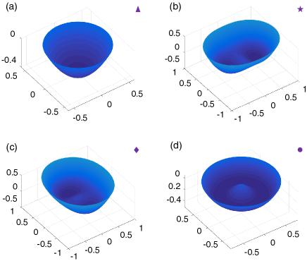
Figure 6: The mean-field landscapes for the corresponding parameter locations indicated by the symbols of (a) triangle, (b) star, (c) diamond, and (d) round in Fig. 1(c).

With the solutions of $\alpha$, the other two order parameters $\beta_{1}$ and $\beta_{2}$ can be straightforwardly derived by employing Eqs. (35)-(40). The complete expressions of $\beta_{1,2}$ are, however, extremely lengthy and we thus do not list them here.

The mean-field solutions are stable only if their associated excitation energies are real. For systems with $n$ bosonic modes, the excitation spectra are obtained by diagonalizing the Hopfield-Bogoliubov matrix superradiance4 ,

$$D_{\text{H}}=\left(\begin{array}[]{cc}\mathbf{H}&\mathbf{K}\\ -\mathbf{K}^{{\dagger}}&-\mathbf{H}^{\text{T}}\end{array}\right)$$ (42)

where $\mathbf{H}$ and $\mathbf{K}$ are the $n\times n$ matrix defined in the Appendix B. For the NP and SP considered in the present system, the diagonalization of the Hopfield-Bogoliubov matrix (42) produces $6$ eigenfrequencies, which are paired with opposite signs $\pm\omega_{i}$ ($i=1,2,3$). The solutions of $\alpha$ and $\beta_{1,2}$, together with their associated eigenfrequencies, determine the whole closed phase diagram.

Figure 6 plot the ME landscapes for four representative points in the $\lambda_{1}-\lambda_{2}$ parameter space indicated by the symbols of triangle, star, diamond and round in Fig. 1(c). It should be noticed that, unlike the NP and SP which minimize $E$, the e-NP [Fig. 6(b)] corresponds to a local maximum of the ME.

Appendix D Steady states and the stability analysis in the open system

In this Section, we detail the derivation of the steady-state solutions of the master equation $\partial_{t}\hat{\rho}=\mathcal{\hat{L}}\hat{\rho}=0$, with which the HP Hamiltonian in the open system is obtained. We remark that in the open system, the HP Hamiltonians for the NP and inverted state are the same as those of the closed system, whereas they have a different form for the SP.

D.1 Superradiant steady state

Utilizing a mean-field decoupling by equating the cavity field operator $\hat{a}$ with its expectation value $\left\langle\hat{a}\right\rangle$, the Hamiltonian (1) can be written as

$$H = \hbar\omega_{0}(\hat{\Lambda}_{1,1}+\hat{\Lambda}_{2,2})+M_{1}\hat{\Lambda}_{1,0}+M_{2}\hat{\Lambda}_{2,0}$$ (43)

$$+M_{1}^{\ast}\hat{\Lambda}_{0,1}+M_{2}^{\ast}\hat{\Lambda}_{0,2}$$

where

$$M_{1} = \frac{\hbar\lambda_{1}}{N(\kappa^{2}+\omega^{2})}\{[\omega\left\langle\hat{\Lambda}_{0,1}\right\rangle+i\kappa\left\langle\hat{\Lambda}_{0,1}\right\rangle+2\sin(\varphi)\cos(\varphi)\omega\left\langle\hat{\Lambda}_{1,0}\right\rangle-2i\cos^{2}(\varphi)\kappa\left\langle\hat{\Lambda}_{0,1}\right\rangle]\lambda_{1}$$ (44)

$$+[\kappa\left\langle\hat{\Lambda}_{0,2}\right\rangle-i\omega\left\langle\hat{\Lambda}_{0,2}\right\rangle+2\sin(\varphi)\cos(\varphi)\kappa\left\langle\hat{\Lambda}_{2,0}\right\rangle+2i\cos^{2}(\varphi)\omega\left\langle\hat{\Lambda}_{0,2}\right\rangle]\lambda_{2}\},$$

$$M_{2} = \frac{i\hbar\lambda_{2}}{N(\kappa^{2}+\omega^{2})}\{[-2\omega\left\langle\hat{\Lambda}_{0,1}\right\rangle\cos^{2}(\varphi)+2i\sin(\varphi)\cos(\varphi)\kappa\left\langle\hat{\Lambda}_{1,0}\right\rangle+(\omega+i\kappa)\left\langle\hat{\Lambda}_{0,1}\right\rangle]\lambda_{1}$$ (45)

$$+[-2\kappa\left\langle\hat{\Lambda}_{0,2}\right\rangle\cos^{2}(\varphi)-2i\omega\sin(\varphi)\cos(\varphi)\left\langle\hat{\Lambda}_{2,0}\right\rangle-(i\omega-\kappa)\left\langle\hat{\Lambda}_{0,2}\right\rangle]\lambda_{2}\}.$$

Note that in writing Eq. (43), the steady state of the cavity field

$$\left\langle\hat{a}\right\rangle = \frac{1}{(\omega+i\kappa)\sqrt{N}}\{[\cos(\varphi)\left\langle\hat{\Lambda}_{1,0}\right\rangle+\sin(\varphi)\left\langle\hat{\Lambda}_{0,1}\right\rangle]\lambda_{1}$$ (46)

$$-[i\cos(\varphi)\left\langle\hat{\Lambda}_{2,0}\right\rangle+i\sin(\varphi)\left\langle\hat{\Lambda}_{0,2}\right\rangle]\lambda_{2}\}$$

has been used. The Hamiltonian (43) produces the equations of motion for the atomic operators $\hat{\Lambda}_{i,j}$ ($i,j=1,2,3$), which are solved under the constraint of the SU(3) atomic symmetry ThreeDicke4 ; ThreeDicke8 , i.e.,

$$\sum_{\mu=0}^{2}\left\langle\hat{\Lambda}_{\mu,\mu}\right\rangle=N,$$ (47)

$$\sum_{\mu=0}^{2}\left\langle\hat{\Lambda}_{\mu,\mu}\right\rangle^{2}+\sum_{\{\mu,\nu\}}\left(3\left|\left\langle\hat{\Lambda}_{\mu,\nu}\right\rangle\right|^{2}-\left\langle\hat{\Lambda}_{\mu,\mu}\right\rangle\left\langle\hat{\Lambda}_{\nu,\nu}\right\rangle\right)=N^{2},$$ (48)

and

$$\frac{9}{2}\sum_{\{\mu,\nu,\rho\}}\left|\left\langle\hat{\Lambda}_{\mu,\nu}\right\rangle\right|^{2}\left(\left\langle\hat{\Lambda}_{\mu,\mu}\right\rangle+\left\langle\hat{\Lambda}_{\nu,\nu}\right\rangle-2\left\langle\hat{\Lambda}_{\rho,\rho}\right\rangle\right)-\frac{1}{2}\prod_{\{\mu,\nu,\rho\}}\left(\left\langle\hat{\Lambda}_{\mu,\mu}\right\rangle+\left\langle\hat{\Lambda}_{\nu,\nu}\right\rangle-2\left\langle\hat{\Lambda}_{\rho,\rho}\right\rangle\right)+27\left|\left\langle\hat{\Lambda}_{0,1}\right\rangle\left\langle\hat{\Lambda}_{1,2}\right\rangle\left\langle\hat{\Lambda}_{2,0}\right\rangle\right|=N^{3},$$ (49)

where the summation $\sum_{\{\mu,\nu\}}$ runs over the pairs $\{\mu,\nu\}=\{0,1\},\{1,2\},\{2,0\}$, while the summation $\sum_{\{\mu,\nu,\rho\}}$ and the product $\prod_{\{\mu,\nu,\rho\}}$ run over the triplets $\{\mu,\nu,\rho\}=\{0,1,2\},\{1,2,0\},\{2,0,1\}$. The solutions reads

$$\left\langle\hat{\Lambda}_{0,1}\right\rangle = \frac{NM_{1}}{\sqrt{4\left|M_{1}\right|^{2}+4\left|M_{2}\right|^{2}+\hbar^{2}\omega_{0}^{2}}},$$ (50)

$$\left\langle\hat{\Lambda}_{0,2}\right\rangle = \frac{NM_{2}}{\sqrt{4\left|M_{1}\right|^{2}+4\left|M_{2}\right|^{2}+\hbar^{2}\omega_{0}^{2}}},$$ (51)

$$\left\langle\hat{\Lambda}_{0,0}\right\rangle = \frac{N}{2}-\frac{N\hbar\omega_{0}}{2\sqrt{4\left|M_{1}\right|^{2}+4\left|M_{2}\right|^{2}+\hbar^{2}\omega_{0}^{2}}},$$ (52)

$$\left\langle\hat{\Lambda}_{1,1}\right\rangle = \frac{N\left|M_{1}\right|^{2}}{2(\left|M_{1}\right|^{2}+\left|M_{2}\right|^{2})}\left(\frac{\hbar\omega_{0}}{\sqrt{4\left|M_{1}\right|^{2}+4\left|M_{2}\right|^{2}+\hbar^{2}\omega_{0}^{2}}}+1\right),$$ (53)

$$\left\langle\hat{\Lambda}_{2,2}\right\rangle = \frac{N\left|M_{2}\right|^{2}}{2(\left|M_{1}\right|^{2}+\left|M_{2}\right|^{2})}\left(\frac{\hbar\omega_{0}}{\sqrt{4\left|M_{1}\right|^{2}+4\left|M_{2}\right|^{2}+\hbar^{2}\omega_{0}^{2}}}+1\right),$$ (54)

$$\left\langle\hat{\Lambda}_{1,2}\right\rangle = \frac{NM_{1}^{\ast}M_{2}}{2(\left|M_{1}\right|^{2}+\left|M_{2}\right|^{2})}\left(\frac{\hbar\omega_{0}}{\sqrt{4\left|M_{1}\right|^{2}+4\left|M_{2}\right|^{2}+\hbar^{2}\omega_{0}^{2}}}+1\right),$$ (55)

and $\left\langle\hat{\Lambda}_{1,0}\right\rangle=\left\langle\hat{\Lambda}_{0,1}\right\rangle^{\ast}$, $\left\langle\hat{\Lambda}_{2,0}\right\rangle=\left\langle\hat{\Lambda}_{0,2}\right\rangle^{\ast}$ and $\left\langle\hat{\Lambda}_{2,1}\right\rangle=\left\langle\hat{\Lambda}_{1,2}\right\rangle^{\ast}$. Eliminating the variables $\left\langle\hat{\Lambda}_{0,1}\right\rangle$, $\left\langle\hat{\Lambda}_{0,2}\right\rangle$, $\left\langle\hat{\Lambda}_{1,0}\right\rangle$ and $\left\langle\hat{\Lambda}_{2,0}\right\rangle$ in Eqs. (44)-(45) by making use of Eqs. (50) -(51), we have

$$\frac{M_{1}}{\hbar\lambda_{1}}=\frac{-M_{1}\lambda_{1}(2i\cos^{2}(\varphi)\kappa-i\kappa-\omega)+M_{2}\lambda_{2}[2i\cos^{2}(\varphi)\omega-i\omega+\kappa]+2M_{1}^{\ast}\lambda_{1}\cos(\varphi)\sin(\varphi)\omega+2M_{2}^{\ast}\lambda_{2}\cos(\varphi)\sin(\varphi)\kappa}{\sqrt{4\left|M_{1}\right|^{2}+4\left|M_{2}\right|^{2}+\hbar^{2}\omega_{0}^{2}}(\kappa^{2}+\omega^{2})}$$ (56)

$$\frac{M_{2}}{\hbar\lambda_{2}}=\frac{-M_{2}\lambda_{2}(2i\cos^{2}(\varphi)\kappa-i\kappa-\omega)-M_{1}\lambda_{1}[2i\cos^{2}(\varphi)\omega-i\omega+\kappa]-2M_{1}^{\ast}\lambda_{1}\cos(\varphi)\sin(\varphi)\kappa+2M_{2}^{\ast}\lambda_{2}\cos(\varphi)\sin(\varphi)\omega}{\sqrt{4\left|M_{1}\right|^{2}+4\left|M_{2}\right|^{2}+\hbar^{2}\omega_{0}^{2}}(\kappa^{2}+\omega^{2})}$$ (57)

By solving Eqs. (56)-(57) and their complex conjugated versions, $M_{1,2}$ can be normally determined. While the expressions of $M_{1,2}$ are too lengthy to be listed here, they are related to the order parameters $\beta_{1,2}$ through the simple algebraic relations

$$\beta_{1} = \frac{\sqrt{2}M_{1}}{\sqrt{\hbar\omega_{0}+\sqrt{4\left|M_{1}\right|^{2}+4\left|M_{2}\right|^{2}+\hbar^{2}\omega_{0}^{2}}}}$$ (58)

$$\beta_{2} = \frac{\sqrt{2}M_{2}}{\sqrt{\hbar\omega_{0}+\sqrt{4\left|M_{1}\right|^{2}+4\left|M_{2}\right|^{2}+\hbar^{2}\omega_{0}^{2}}}}.$$ (59)

With the obtained $\beta_{1,2}$ and taking into consideration the fluctuation Hamiltonian (30), the matrices $\mathbf{H}$ and $\mathbf{K}$ are uniquely fixed.

D.2 Third quantization and the stability analysis

The third quantization approach exactly solves the Lindblad master equation for an arbitrary quadratic system of $n$ bosons/fermions with linear bath operators ThirdQuant1 ; ThirdQuant2 , and is hence suitable for the stability analysis around the obtained non-equilibrium steady states. We here skip the details of this method in quantizing the density operator, and focus on the most relevant steps in analyzing the system stability.

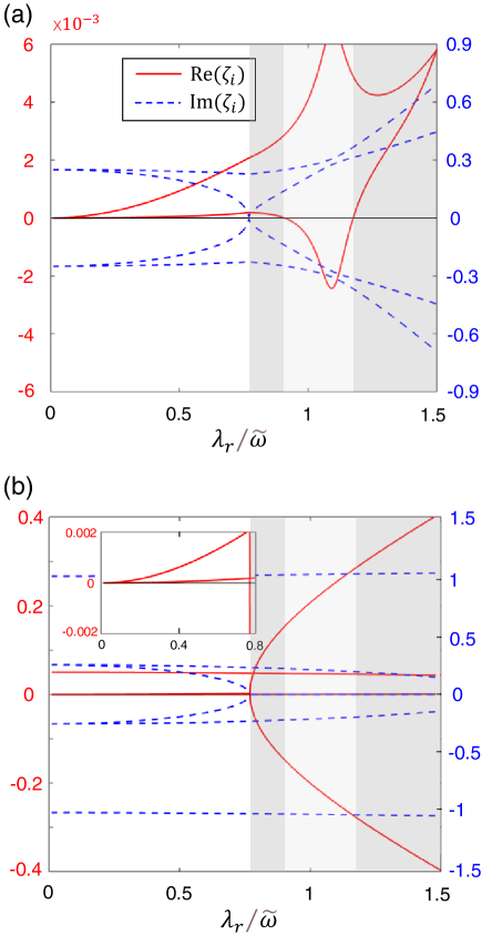
Figure 7: The real (red solid) and imaginary (blue dashed) parts of the rapidities $\zeta_{i}$ on top of the (a) superradiant and (b) normal phases. As the coupling strength $\lambda_{r}$ increases, the system traverses the regions of multi-phase coexistence of NP+SP (white), SP (dark grey), OS (light grey), and SP (dark grey). The parameters are chosen as $\varphi=0.22\pi$, $\lambda_{2}/\lambda_{1}=0.41$, $\omega=4\omega_{0}=2\tilde{\omega}$ and $\kappa=0.1\tilde{\omega}$. 

Under the framework of the third quantization, the dynamical property of the steady states is captured by the shape matrix of the Liouvillian,

$$\chi=\frac{1}{2}\left(\begin{array}[]{cc}i\mathbf{H}^{\ast}-\mathbf{N}^{\ast}+\mathbf{M}&-2\mathbf{K}-\mathbf{L}+\mathbf{L}^{\text{T}}\\ 2i\mathbf{K}^{\ast}-\mathbf{L}^{\ast}+\mathbf{L}^{{\dagger}}&-i\mathbf{H}-\mathbf{N}+\mathbf{M}^{\ast}\end{array}\right)$$ (60)

where $\mathbf{H}$ and $\mathbf{K}$ are defined in the Appendix B, and the other three matrices are given by

$$\mathbf{M=}\underline{l}_{1}\otimes\underline{l}_{1}^{\ast}\text{, }\mathbf{N=}\underline{l}_{2}\otimes\underline{l}_{2}^{\ast}\text{, }\mathbf{L}=\underline{l}_{1}\otimes\underline{l}_{2}^{\ast}.$$ (61)

The matrices $\underline{l}_{1,2}$ in Eq. (61) are defined through the linear Lindblad bath operators in the form of

$$L=\underline{l}_{1}\cdot\underline{a}+\underline{l}_{2}\cdot\underline{a^{{\dagger}}}.$$ (62)

Given that the bath operator for our model is $L=\sqrt{\kappa}\hat{c}$, we have the operator basis $\underline{a}=(\hat{c},\hat{d}_{1},\hat{d}_{2})^{\text{T}}$ and the corresponding matrices $\underline{l}_{1}=(\sqrt{\kappa},0,0)^{\text{T}}$ and $\underline{l}_{2}=(0,0,0)^{\text{T}}$ for the SP and NP, leading to

$$\mathbf{M}_{\text{N/S}}=\text{diag}(\kappa,0,0)\text{, }\mathbf{N}_{\text{N/S}}=\mathbf{L}_{\text{N/S}}=\mathbf{0}_{3\times 3}$$ (63)

whereas for the inverted state, we have $\underline{a}=(\hat{c},\hat{d}_{0})^{\text{T}}$, $\underline{l}_{1}=(\sqrt{\kappa},0)^{\text{T}}$, and$\ \underline{l}_{2}=(0,0)^{\text{T}}$, resulting in

$$\mathbf{M}_{\text{I}}=\text{diag}(\kappa,0)\text{, }\mathbf{N}_{\text{I}}=\mathbf{L}_{\text{I}}=\mathbf{0}_{2\times 2}.$$ (64)

The eigenvalues of the shape matrix $\chi$, dubbed rapidities and represented by $\zeta_{i}$, are negatively related to the eigenvalues of the Liouvillian and thus play the role of excitation energies in the closed system. It follows that the real part of $\zeta_{i}$ determines the stability of the corresponding steady state and, the imaginary part represents the oscillation frequency of the fluctuations. The steady state is stable if and only if the real part of all the rapidities are nonnegative, i.e., min(Re$\zeta_{i}$) $\geqslant 0$. For parameters region where both NP and SP are unstable, we should further integrate the equations of motion starting from arbitrary initial conditions to identify possible limit-cycle attractors. In Fig. 7, we plot the rapidities on top of the NP and SP for some representative parameters.

Appendix E Mean-field equations of motion

According to the master equation $\partial_{t}\hat{\rho}=\mathcal{\hat{L}}\hat{\rho}$, we can obtain the equation of motion for the expectation of a general operator $\mathcal{\hat{O}}$,

$$\frac{d}{dt}\left\langle\mathcal{\hat{O}}\right\rangle=-\frac{i}{\hbar}\left\langle\left[\mathcal{\hat{O}},\hat{H}\right]\right\rangle-\kappa\left\{\left\langle\left[\mathcal{\hat{O}},\hat{a}^{{\dagger}}\right]\hat{a}\right\rangle-\left\langle\hat{a}^{{\dagger}}\left[\mathcal{\hat{O}},\hat{a}\right]\right\rangle\right\}.$$ (65)

For our model, the operator $\mathcal{\hat{O}}$ is chosen as the pseudospin operators $\hat{\Lambda}_{i,j}$ and cavity field operator $\hat{a}$. Applying the mean-field decoupling $\left\langle\hat{\Lambda}_{i,j}\hat{a}\right\rangle\approx\left\langle\hat{\Lambda}_{i,j}\right\rangle\left\langle\hat{a}\right\rangle$, we can derive the closed set of equations of motion

$$\frac{d}{dt}\left\langle\hat{a}\right\rangle = (i\hbar\omega-\kappa)\left\langle\hat{a}\right\rangle-\frac{i\hbar\lambda_{1}[\cos(\varphi)\left\langle\hat{\Lambda}_{1,0}\right\rangle+\sin(\varphi)\left\langle\hat{\Lambda}_{0,1}\right\rangle]-i\hbar\lambda_{2}[\cos(\varphi)\left\langle\hat{\Lambda}_{2,0}\right\rangle+\sin(\varphi)\left\langle\hat{\Lambda}_{0,2}\right\rangle]}{\sqrt{N}}$$

$$\frac{d}{dt}\left\langle\hat{a}^{{\dagger}}\right\rangle = (-i\hbar\omega-\kappa)\left\langle\hat{a}\right\rangle+\frac{i\hbar\lambda_{1}[\cos(\varphi)\left\langle\hat{\Lambda}_{0,1}\right\rangle+\sin(\varphi)\left\langle\hat{\Lambda}_{1,0}\right\rangle]-i\hbar\lambda_{2}[\cos(\varphi)\left\langle\hat{\Lambda}_{0,2}\right\rangle+\sin(\varphi)\left\langle\hat{\Lambda}_{2,0}\right\rangle]}{\sqrt{N}}$$

$$\frac{d}{dt}\left\langle\hat{\Lambda}_{0,0}\right\rangle = \frac{-i\hbar\lambda_{1}\{-\left\langle\hat{\Lambda}_{0,1}\right\rangle[\sin(\varphi)\left\langle\hat{a}\right\rangle+\cos(\varphi)\left\langle\hat{a}^{{\dagger}}\right\rangle]+\left\langle\hat{\Lambda}_{1,0}\right\rangle[\sin(\varphi)\left\langle\hat{a}^{{\dagger}}\right\rangle+\cos(\varphi)\left\langle\hat{a}\right\rangle]\}}{\sqrt{N}}$$

$$+\frac{\hbar\lambda_{2}\{-\left\langle\hat{\Lambda}_{2,0}\right\rangle[\sin(\varphi)\left\langle\hat{a}\right\rangle-\cos(\varphi)\left\langle\hat{a}^{{\dagger}}\right\rangle]+\left\langle\hat{\Lambda}_{0,2}\right\rangle[-\sin(\varphi)\left\langle\hat{a}^{{\dagger}}\right\rangle+\cos(\varphi)\left\langle\hat{a}\right\rangle]\}}{\sqrt{N}}$$

$$\frac{d}{dt}\left\langle\hat{\Lambda}_{1,1}\right\rangle = \frac{-i\hbar\lambda_{1}\{\left\langle\hat{\Lambda}_{1,0}\right\rangle[\sin(\varphi)\left\langle\hat{a}\right\rangle+\cos(\varphi)\left\langle\hat{a}^{{\dagger}}\right\rangle]-\left\langle\hat{\Lambda}_{0,1}\right\rangle[\sin(\varphi)\left\langle\hat{a}^{{\dagger}}\right\rangle+\cos(\varphi)\left\langle\hat{a}\right\rangle]\}}{\sqrt{N}}$$

$$\frac{d}{dt}\left\langle\hat{\Lambda}_{2,2}\right\rangle = \frac{\hbar\lambda_{2}\{\left\langle\hat{\Lambda}_{2,0}\right\rangle[\sin(\varphi)\left\langle\hat{a}\right\rangle-\cos(\varphi)\left\langle\hat{a}^{{\dagger}}\right\rangle]-\left\langle\hat{\Lambda}_{0,2}\right\rangle[-\sin(\varphi)\left\langle\hat{a}^{{\dagger}}\right\rangle+\cos(\varphi)\left\langle\hat{a}\right\rangle]\}}{\sqrt{N}}$$

$$\frac{d}{dt}\left\langle\hat{\Lambda}_{1,2}\right\rangle = \frac{i\hbar\lambda_{1}\left\langle\hat{\Lambda}_{0,2}\right\rangle[\sin(\varphi)\left\langle\hat{a}^{{\dagger}}\right\rangle+\cos(\varphi)\left\langle\hat{a}\right\rangle]+\hbar\lambda_{2}\left\langle\hat{\Lambda}_{1,0}\right\rangle[\sin(\varphi)\left\langle\hat{a}\right\rangle-\cos(\varphi)\left\langle\hat{a}^{{\dagger}}\right\rangle]}{\sqrt{N}}$$

$$\frac{d}{dt}\left\langle\hat{\Lambda}_{0,1}\right\rangle = -i\hbar\omega_{0}\left\langle\hat{\Lambda}_{0,1}\right\rangle-\frac{i\hbar\lambda_{1}(\left\langle\hat{\Lambda}_{0,0}\right\rangle-\left\langle\hat{\Lambda}_{1,1}\right\rangle)[\sin(\varphi)\left\langle\hat{a}\right\rangle+\cos(\varphi)\left\langle\hat{a}^{{\dagger}}\right\rangle]}{\sqrt{N}}-\frac{\hbar\lambda_{2}\left\langle\hat{\Lambda}_{2,1}\right\rangle[\sin(\varphi)\left\langle\hat{a}\right\rangle-\cos(\varphi)\left\langle\hat{a}^{{\dagger}}\right\rangle]}{\sqrt{N}}$$

$$\frac{d}{dt}\left\langle\hat{\Lambda}_{0,2}\right\rangle = -i\hbar\omega_{0}\left\langle\hat{\Lambda}_{0,2}\right\rangle+\frac{\hbar\lambda_{2}(\left\langle\hat{\Lambda}_{0,0}\right\rangle-\left\langle\hat{\Lambda}_{2,2}\right\rangle)[\sin(\varphi)\left\langle\hat{a}\right\rangle-\cos(\varphi)\left\langle\hat{a}^{{\dagger}}\right\rangle]}{\sqrt{N}}+\frac{i\hbar\lambda_{1}\left\langle\hat{\Lambda}_{1,2}\right\rangle[\sin(\varphi)\left\langle\hat{a}\right\rangle+\cos(\varphi)\left\langle\hat{a}^{{\dagger}}\right\rangle]}{\sqrt{N}}$$

$$\frac{d}{dt}\left\langle\hat{\Lambda}_{2,1}\right\rangle = \frac{-i\hbar\lambda_{1}\left\langle\hat{\Lambda}_{2,0}\right\rangle[\sin(\varphi)\left\langle\hat{a}\right\rangle+\cos(\varphi)\left\langle\hat{a}^{{\dagger}}\right\rangle]+\hbar\lambda_{2}\left\langle\hat{\Lambda}_{0,1}\right\rangle[\sin(\varphi)\left\langle\hat{a}^{{\dagger}}\right\rangle-\cos(\varphi)\left\langle\hat{a}\right\rangle]}{\sqrt{N}}$$

$$\frac{d}{dt}\left\langle\hat{\Lambda}_{1,0}\right\rangle = i\hbar\omega_{0}\left\langle\hat{\Lambda}_{1,0}\right\rangle+\frac{i\hbar\lambda_{1}(\left\langle\hat{\Lambda}_{0,0}\right\rangle-\left\langle\hat{\Lambda}_{1,1}\right\rangle)[\sin(\varphi)\left\langle\hat{a}^{{\dagger}}\right\rangle+\cos(\varphi)\left\langle\hat{a}\right\rangle]}{\sqrt{N}}-\frac{\hbar\lambda_{2}\left\langle\hat{\Lambda}_{1,2}\right\rangle[\sin(\varphi)\left\langle\hat{a}^{{\dagger}}\right\rangle-\cos(\varphi)\left\langle\hat{a}\right\rangle]}{\sqrt{N}}$$

$$\frac{d}{dt}\left\langle\hat{\Lambda}_{2,0}\right\rangle = -i\hbar\omega_{0}\left\langle\hat{\Lambda}_{2,0}\right\rangle+\frac{\hbar\lambda_{2}(\left\langle\hat{\Lambda}_{0,0}\right\rangle-\left\langle\hat{\Lambda}_{2,2}\right\rangle)[\sin(\varphi)\left\langle\hat{a}^{{\dagger}}\right\rangle-\cos(\varphi)\left\langle\hat{a}\right\rangle]}{\sqrt{N}}+\frac{i\hbar\lambda_{1}\hat{\Lambda}_{2,1}[\sin(\varphi)\left\langle\hat{a}^{{\dagger}}\right\rangle+\cos(\varphi)\left\langle\hat{a}\right\rangle]}{\sqrt{N}}$$

References

- (1) R. H. Dicke, Coherence in Spontaneous Radiation Processes, Phys. Rev. 93, 99 (1954).
- (2) P. Kirton, M. M. Roses, J. Keeling, and E. G. Dalla Torre, Introduction to the Dicke Model: From Equilibrium to Nonequilibrium, and Vice Versa, Adv. Quantum Technol. 2, 1800043 (2019).
- (3) K. Hepp and E. H. Lieb, On the superradiant phase transition for molecules in a quantized radiation field: the dicke maser model, Ann. Phys. (N.Y.) 76, 360 (1973).
- (4) Y. K. Wang and F. T. Hioe, Phase Transition in the Dicke Model of Superradiance, Phys. Rev. A 7, 831 (1973).
- (5) M. Gross and S. Haroche, Superradiance: An essay on the theory of collective spontaneous emission, Phys. Rep. 93, 301 (1982).
- (6) C. Emary and T. Brandes, Chaos and the quantum phase transition in the Dicke model, Phys. Rev. E 67, 066203 (2003).
- (7) K. Baumann, C. Guerlin, F. Brennecke, and T. Esslinger, Dicke quantum phase transition with a superfluid gas in an optical cavity, Nature (London) 464, 1301 (2010).
- (8) K. Baumann, R. Mottl, F. Brennecke, and T. Esslinger, Exploring Symmetry Breaking at the Dicke Quantum Phase Transition, Phys. Rev. Lett. 107, 140402 (2011).
- (9) F. Brennecke, R. Mottl, K. Baumann, R. Landig, T. Donner, and T. Esslinger, Real-time observation of fluctuations at the driven-dissipative Dicke phase transition, Proc. Natl. Acad. Sci. USA 110, 11763 (2013).
- (10) D. Nagy, G. Kóya, G. Szirmai, and P. Domokos, Dicke-Model Phase Transition in the Quantum Motion of a Bose-Einstein Condensate in an Optical Cavity, Phys. Rev. Lett. 104, 130401 (2010).
- (11) D. Nagy, G. Szirmai, and P. Domokos, Critical exponent of a quantum-noise-driven phase transition: The open-system Dicke model, Phys. Rev. A 84, 043637 (2011).
- (12) G. Barontini, R. Labouvie, F. Stubenrauch, A. Vogler, V. Guarrera, and H. Ott, Controlling the Dynamics of an Open Many-Body Quantum System with Localized Dissipation, Phys. Rev. Lett. 110, 035302 (2013).
- (13) J. Klinder, H. Keßer, M. Wolke, L. Mathey, and A. Hemmerich, Dynamical phase transition in the open Dicke model, Proc. Natl. Acad. Sci. U.S.A. 112, 3290 (2015).
- (14) H. Ritsch, P. Domokos, F. Brennecke, and T. Esslinger, Cold atoms in cavity-generated dynamical optical potentials, Rev. Mod. Phys. 85, 553 (2013).
- (15) F. Mivehvar, F. Piazza, T. Donner, and H. Ritsch, Cavity QED with quantum gases: new paradigms in many-body physics, Advances in Physics 70, 1 (2021).
- (16) J. Gelhausen and M. Buchhold, Dissipative Dicke model with collective atomic decay: Bistability, noise-driven activation, and the nonthermal first-order superradiance transition, Phys. Rev. A 97, 023807 (2018).
- (17) N. Dogra, M. Landini, K. Kroeger, L. Hruby, T. Donner, and T. Esslinger, Dissipation-induced structural instability and chiral dynamics in a quantum gas, Science 366, 1496 (2019).
- (18) E. I. Rodríguez Chiacchio and A. Nunnenkamp, Dissipation-Induced Instabilities of a Spinor Bose-Einstein Condensate Inside an Optical Cavity, Phys. Rev. Lett. 122, 193605 (2019).
- (19) B. Buča and D. Jaksch, Dissipation Induced Nonstationarity in a Quantum Gas, Phys. Rev. Lett. 123, 260401 (2019).
- (20) F. Damanet, Andrew J. Daley, and J. Keeling, Atom-only descriptions of the driven-dissipative Dicke model, Phys. Rev. A 99, 033845 (2019).
- (21) A. Patra, Boris L. Altshuler, and Emil A. Yuzbashyan, Driven-dissipative dynamics of atomic ensembles in a resonant cavity: Nonequilibrium phase diagram and periodically modulated superradiance, Phys. Rev. A 99, 033802 (2019).
- (22) Kevin C. Stitely, Stuart J. Masson, A. Giraldo, B. Krauskopf, and S. Parkins, Superradiant switching, quantum hysteresis, and oscillations in a generalized Dicke model, Phys. Rev. A 102, 063702 (2020).
- (23) F. Reiter, T. L. Nguyen, Jonathan P. Home, and Susanne F. Yelin, Cooperative Breakdown of the Oscillator Blockade in the Dicke Model, Phys. Rev. Lett. 125, 233602 (2020).
- (24) J. Fan, G. Chen, and S. Jia, Atomic self-organization emerging from tunable quadrature coupling, Phys. Rev. A 101, 063627 (2020).
- (25) C. J. Zhu, L. L. Ping, Y. P. Yang, and G. S. Agarwal, Squeezed Light Induced Symmetry Breaking Superradiant Phase Transition, Phys. Rev. Lett. 124, 073602 (2020).
- (26) S. Samimi and M. M. Golshan, Switchability of multimodal optical phases in a leaky and nonlinear quantum cavity, Phys. Rev. A 103, 033712 (2021).
- (27) M. Boneberg, I. Lesanovsky, and Federico Carollo, Quantum fluctuations and correlations in open quantum Dicke models, Phys. Rev. A 106, 012212 (2022).
- (28) J. Larson and Th. K. Mavrogordatos, The Jaynes–Cummings Model and Its Descendants, (IOP Publishing Ltd, 2021).
- (29) J. Larson and E. K. Irish, Some remarks on superradiant phase transitions in light-matter systems, J. Phys. A: Math. Theor. 50, 174002 (2017).
- (30) Victor V. Albert, Gregory D. Scholes, and P. Brumer, Symmetric rotating-wave approximation for the generalized single-mode spin-boson system, Phys. Rev. A 84, 042110 (2011).
- (31) A. Ridolfo, M. Leib, S. Savasta, and M. J. Hartmann, Photon Blockade in the Ultrastrong Coupling Regime, Phys. Rev. Lett. 109, 193602 (2012).
- (32) A. Ridolfo, S. Savasta, and M. J. Hartmann, Nonclassical Radiation from Thermal Cavities in the Ultrastrong Coupling Regime, Phys. Rev. Lett. 110, 163601 (2013).
- (33) J. Keeling, M. J. Bhaseen, and B. D. Simons, Collective Dynamics of Bose-Einstein Condensates in Optical Cavities, Phys. Rev. Lett. 105, 043001 (2010).
- (34) M. J. Bhaseen, J. Mayoh, B. D. Simons, and J. Keeling, Dynamics of nonequilibrium Dicke models, Phys. Rev. A 85, 013817 (2012).
- (35) M. Soriente, T. Donner, R. Chitra, and O. Zilberberg, Dissipation-Induced Anomalous Multicritical Phenomena, Phys. Rev. Lett. 120, 183603 (2018).
- (36) P. Kirton and J. Keeling, Superradiant and lasing states in driven-dissipative Dicke models, New J. Phys. 20, 015009 (2019).
- (37) Kevin C. Stitely, A. Giraldo, B. Krauskopf, and S. Parkins, Nonlinear semiclassical dynamics of the unbalanced, open Dicke model, Phys. Rev. Research 2, 033131 (2020).
- (38) M. Soriente, R. Chitra, and O. Zilberberg, Distinguishing phases using the dynamical response of driven-dissipative light-matter systems, Phys. Rev. A 101, 023823 (2020).
- (39) M. Soriente, Toni L. Heugel, K. Omiya, R. Chitra, and O. Zilberberg, Distinctive class of dissipation-induced phase transitions and their universal characteristics, Phys. Rev. Research 3, 023100 (2021).
- (40) Kevin C. Stitely, A. Giraldo, B. Krauskopf, and S. Parkins, Lasing and counter-lasing phase transitions in a cavity-QED system, Phys. Rev. Research 4, 023101 (2022).
- (41) F. Dimer, B. Estienne, A. S. Parkins, and H. J. Carmichael, Proposed realization of the Dicke-model quantum phase transition in an optical cavity QED system, Phys. Rev. A 75, 013804 (2007).
- (42) Z. Zhiqiang, C. H. Lee, R. Kumar, K. J. Arnold, S. J. Masson, A. S. Parkins, and M. D. Barrett, Non-equilibrium phase transition in a spin one Dicke model, Optica 4, 424 (2017).
- (43) Z. Zhang, C. H. Lee, R. Kumar, K. J. Arnold, S. J. Masson, A. L. Grimsmo, A. S. Parkins, and M. D. Barrett, Dicke-model simulation via cavity-assisted Raman transitions, Phys. Rev. A 97, 043858 (2018).
- (44) F. Ferri, R. Rosa-Medina, F. Finger, N. Dogra, M. Soriente, O. Zilberberg, T. Donner, and T. Esslinger, Phys. Rev. X 11, 041046 (2021).
- (45) K.-J. Boller, A. Imamoğlu, and S. E. Harris, Observation of Electromagnetically Induced Transparency, Phys. Rev. Lett. 66, 2593 (1991).
- (46) M. Fleischhauer, A. Imamoglu, and J. P. Marangos, Electromagnetically induced transparency: Optics in coherent media, Rev. Mod. Phys. 77, 633 (2005).
- (47) M. O. Scully, S.-Y. Zhu, and A. Gavrielides, Degenerate Quantum-Beat Laser: Lasing without Inversion and Inversion without Lasing, Phys. Rev. Lett. 62, 2813 (1989).
- (48) J. Mompart and R. Corbalán, Lasing without inversion, J. Opt. B: Quantum Semiclassical Opt. 2, R7 (2000).
- (49) P. W. Milonni, Semiclassical and quantum-electrodynamical approaches in nonrelativistic radiation theory, Physics Reports 25, 1 (1976).
- (50) D. A. Cardimona, M. G. Raymer, and C. R. Stroud, Jr., Steady-state quantum interference in resonance fluorescence, Journal of Physics B: Atomic and Molecular Physics 15, 55 (1982).
- (51) M. M. Cola, D. Bigerni, and N. Piovella, Recoil-induced subradiance in an ultracold atomic gas, Phys. Rev. A 79, 053622 (2009).
- (52) M. Hayn, C. Emary, and T. Brandes, Superradiant phase transition in a model of three-level- systems interacting with two bosonic modes, Phys. Rev. A 86, 063822 (2012).
- (53) A. Baksic, P. Nataf, and C. Ciuti, Superradiant phase transitions with three-level systems, Phys. Rev. A 87, 023813 (2013).
- (54) O. Castaños, S. Cordero, R. López-Peña, and E. Nahmad-Achar, Single and collective regimes in three-level systems interacting with a one-mode electromagnetic field, Journal of Physics: Conference Series 512, 012006 (2014).
- (55) P. Wolf, S. C. Schuster, D. Schmidt, S. Slama, and C. Zimmermann, Observation of Subradiant Atomic Momentum States with Bose-Einstein Condensates in a Recoil Resolving Optical Ring Resonator, Phys. Rev. Lett. 121, 173602 (2018).
- (56) J. Skulte, P. Kongkhambut, H. Keer, A. Hemmerich, L. Mathey, and Jayson G. Cosme, Parametrically driven dissipative three-level Dicke model, Phys. Rev. A 104, 063705 (2021).
- (57) P. Kongkhambut, H. Keer, J. Skulte, L. Mathey, Jayson G. Cosme, and A. Hemmerich, Realization of a Periodically Driven Open Three-Level Dicke Model, Phys. Rev. Lett. 127, 253601 (2021).
- (58) Y. -Y. Chen, J. -J. Cheng, C. Ye, and Y. Li, Enantiodetection of cyclic three-level chiral molecules in a driven cavity, Phys. Rev. A 4, 013100 (2022).
- (59) S. Samimi and M. M. Golshan, Characteristics of superradiant optical phases occurring in the system of nondegenerate atoms and radiation that are interacting inside a nonlinear quantum cavity, Phys. Rev. A 105, 053702 (2022).
- (60) R. Lin, R. Rosa-Medina, F. Ferri, F. Finger, K. Kroeger, T. Donner, T. Esslinger, and R. Chitra, Dissipation-Engineered Family of Nearly Dark States in Many-Body Cavity-Atom Systems, Phys. Rev. Lett. 128, 153601 (2022).
- (61) H. Georgi, Lie Algebras In Particle Physics from Isospin To Unified Theories (Taylor & Francis, Boca Raton, 2000).
- (62) M. Tavis and F. W. Cummings, Exact Solution for an N-Molecule—Radiation-Field Hamiltonian, Phys. Rev. 170, 379 (1968).
- (63) T. Prosen, Third quantization: a general method to solve master equations for quadratic open Fermi systems, New J. Phys. 10, 043026 (2008).
- (64) T. Prosen and T. H. Seligman, Quantization over boson operator spaces, J. Phys. A 43, 392004 (2010).
- (65) To be clarity, we further confine the value range of to be for the open model. The parameter out of this range can be reset by utilizing the following symmetry transformations: , , and .
- (66) S. Haroche, and J. M. Raimond, Exploring the Quantum: Atoms, Cavities, and Photons. (Oxford university press, Oxford, 2006).
- (67) S. Diehl, A. Micheli, A. Kantian, B. Kraus, H. P. Büchler, and P. Zoller, Quantum states and phases in driven open quantum systems with cold atoms, Nat. Phys. 4, 878 (2008).
- (68) D. Finkelstein-Shapiro, S. Felicetti, T. Hansen, T. Pullerits, and A. Keller, Classification of dark states in multilevel dissipative systems, Phys. Rev. A 99, 053829 (2019).
- (69) R. Jozsa, Fidelity for Mixed Quantum States, Journal of Modern Optics 41, 2315 (1994).
- (70) B. Schumacher, Sending entanglement through noisy quantum channels, Phys. Rev. A 54, 2614 (1996).
- (71) D. A. Steck, Rubidium 87 D line Data, available online at http://steck.us/alkalidata (revision 2.1.4, 23 December 2010).
- (72) T. Holstein, and H. Primakoff, Field dependence of the intrinsic domain magnetization of a ferromagnet, Phys. Rev. 58, 1098 (1949).
- (73) A. Klein, and E. R. Marshalek, Boson realizations of Lie algebras with applications to nuclear physics, Rev. Mod. Phys. 63, 375 (1991).