A Tale of Two Graphs: Freezing and Denoising Graph Structures for Multimodal Recommendation

Abstract.

Multimodal recommender systems utilizing multimodal features (e.g., images and textual descriptions) typically show better recommendation accuracy than general recommendation models based solely on user-item interactions. Generally, prior work fuses multimodal features into item ID embeddings to enrich item representations, thus failing to capture the latent semantic item-item structures. In this context, LATTICE proposes to learn the latent structure between items explicitly and achieves state-of-the-art performance for multimodal recommendations. However, we argue the latent graph structure learning of LATTICE is both inefficient and unnecessary. Experimentally, we demonstrate that freezing its item-item structure before training can also achieve competitive performance. Based on this finding, we propose a simple yet effective model, dubbed as FREEDOM, that FREEzes the item-item graph and DenOises the user-item interaction graph simultaneously for Multimodal recommendation. Theoretically, we examine the design of FREEDOM through a graph spectral perspective and demonstrate that it possesses a tighter upper bound on the graph spectrum. In denoising the user-item interaction graph, we devise a degree-sensitive edge pruning method, which rejects possibly noisy edges with a high probability when sampling the graph. We evaluate the proposed model on three real-world datasets and show that FREEDOM can significantly outperform current strongest baselines. Compared with LATTICE, FREEDOM achieves an average improvement of 19.07% in recommendation accuracy while reducing its memory cost up to 6$\times$ on large graphs. The source code is available at: https://github.com/enoche/FREEDOM.

1. Introduction

The increasing availability of multimodal information (e.g., images, texts and videos) associated with items enables users to have a more in-depth and comprehensive understanding of the items they are interested in. Consequently, multimodal recommender systems (MRSs) leveraging multimodal information are a recent trend in capturing the preferences of users for accurate item recommendations in online platforms, such as e-commerce and instant video platforms, etc. Studies (He and McAuley, 2016b; Zhang et al., 2021) demonstrate that MRSs usually have better performance than general recommendation models which only utilize the historical user-item interactions.

The primary challenge in MRSs is how to effectively integrate the multimodal information into the collaborative filtering (CF) framework. Conventional studies either fuse the projected low-dimensional multimodal features with the ID embeddings of items via concatenation, summation operations (He and McAuley, 2016b; Liu et al., 2017) or leverage attention mechanisms to capture users’ preferences on items (Chen et al., 2017; Liu et al., 2019; Chen et al., 2019). The surge of research on graph-based recommendations (Wu et al., 2020; Zhang et al., 2022; Zhou et al., 2023b, a) inspires a line of work (Wei et al., 2020; Wang et al., 2021b; Zhang et al., 2021; Zhou et al., 2023e) that exploits the power of graph neural networks (GNNs) to capture the high-order semantics between multimodal features and user-item interactions. Specifically, MMGCN (Wei et al., 2019) utilizes graph convolutional networks (GCNs) to propagate and aggregate information on every modality of the item. On top of MMGCN, GRCN (Wei et al., 2020) refines the user-item bipartite graph by weighing the user-item edges according to the affinity between user preference and item content. To achieve better recommendation performance, researchers exploit auxiliary graph structures to explicitly capture the relations between users or items. For instance, DualGNN (Wang et al., 2021b) constructs the user-user relation graph to smoothen users’ preferences with their neighbors via GNNs. Nonetheless, the authors of LATTICE (Zhang et al., 2021) argue that the latent item-item structures underlying the multimodal contents of items could lead to better representation learning. Hence, LATTICE first dynamically constructs a latent item-item graph by considering raw and projected multimodal features learned from multi-layer perceptrons (MLPs). It then performs graph convolutions on the constructed latent item-item graph to explicitly incorporate item relationships into representation learning. As a result, LATTICE could exploit both the high-order interaction semantic from the user-item graph and the latent item content semantic from the item-item structure. Although this paradigm turns out to be effective, it poses a prohibitive cost by requiring computation and memory quadratic in the number of items.

In this paper, we first experimentally disclose that the item-item structure learning of LATTICE is dispensable. Specifically, we build an item-item graph directly from the raw multimodal contents of items and freeze it in training LATTICE. Under the same evaluation settings and datasets of LATTICE, our empirical experiments in Table 1 show that LATTICE with frozen item-item graph structures (i.e., LATTICE-Frozen) gains slightly better performance on two out of three datasets. To further refine the structures in both user-item bipartite graph and the item-item graph, we propose a graph structures FREEzing and DenOising Multimodal model for recommendation, dubbed as FREEDOM. To be specific, the item-item graph constructed by LATTICE retains the affinities between items as the edge weights, which may be noisy as the multimodal features are extracted from general pre-trained models (e.g., Convolutional Neural Networks or Transformers). FREEDOM discretizes the weighted item-item graph into an unweighted one to enable information propagation in GCNs only depending on graph structure. For the user-item graph, we further introduce a degree-sensitive edge pruning technique to denoise its structure to remove the noise caused by unintentional interactions or bribes (Zhou et al., 2022). Inspired by (Chen et al., 2020), we sample edges following a multinomial distribution with pre-calculated parameters to construct a sparsified subgraph. Finally, FREEDOM learns the representations of users and items by integrating the unweighted item-item graph and the sparsified user-item subgraph. We analyze FREEDOM via a spectral perspective to demonstrate that FREEDOM is capable of achieving a tighter low-pass filter. We conduct comprehensive experiments on three real-world datasets to show that our proposed model can significantly outperform the state-of-the-art methods in terms of recommendation accuracy.

Table 1. LATTICE with frozen item-item graph structures (i.e., LATTICE-Frozen) shows slightly better performance than its original version on Baby and Sports in terms of Recall and NDCG (Refer Section 5 for detailed experiment settings).

Dataset	Metric	LATTICE	LATTICE-Frozen
Baby	R@10	0.0547	0.0551
	R@20	0.0850	0.0873
	N@10	0.0292	0.0291
	N@20	0.0370	0.0373
Sports	R@10	0.0620	0.0626
	R@20	0.0953	0.0964
	N@10	0.0335	0.0336
	N@20	0.0421	0.0423
Clothing	R@10	0.0492	0.0434
	R@20	0.0733	0.0635
	N@10	0.0268	0.0227
	N@20	0.0330	0.0279

2. Related Work

2.1. Multimodal Recommendation

Multimodal recommendation models utilize deep or graph learning techniques to effectively incorporate the multimodal information of items into the classic CF paradigm for better recommendation performance. Previous work (He and McAuley, 2016b; Liu et al., 2017) extends the BPR method (Rendle et al., 2009) by fusing the visual and/or style content of items with their ID embeddings and obtains a considerable performance boost. To further differentiate users’ preferences on multimodal information, attention mechanisms are exploited in multimodal recommendation models. For instance, VECF (Chen et al., 2019) utilizes the VGG model (Simonyan and Zisserman, 2014) to perform pre-segmentation on images and captures the user’s attention on different image regions. MAML (Liu et al., 2019) uses a two-layer neural network to capture the user’s preference for textual and visual features of an item. Under the surge of GNNs applied in recommendation systems (Wu et al., 2020), researchers are inspired to inject high-order semantics into user/item representation learning via GNNs. MMGCN (Wei et al., 2019) adopts the message passing mechanism of GCNs and constructs a modality-specific user-item bipartite graph, which can capture the information from multi-hop neighbors to enhance the user and item representations. Following MMGCN, GRCN (Wei et al., 2020) introduces a graph refine layer to refine the structure of the user-item interaction graph by identifying the noise edges and corrupting the false-positive edges. In DualGNN (Wang et al., 2021b), the authors argue that users’ preferences may dynamically evolve with time. They introduce a user co-occurrence graph with a preference learning module to capture the user’s preference for features from different modalities of an item. However, the aforementioned models mine the semantic information between items in an implicit manner and may lead to inferior performance. To this end, LATTICE (Zhang et al., 2021) explicitly constructs item-item relation graphs for each modality and fuses them together to obtain a latent item-item graph. It then dynamically updates the item-item graph with projected multimodal features from MLPs and achieves state-of-the-art recommendation accuracy. Recently, we also see an emerging of applying self-supervised learning in multimodal recommendations (Tao et al., 2022; Zhou et al., 2023c). For an in-depth exploration of multimodal recommender systems, we recommend consulting the comprehensive survey conducted by  (Zhou et al., 2023d).

2.2. Denoising Graph Structures

Studies on denoising graph structures can be roughly categorized as either permanent or temporary edge pruning. Edges are either pruned or retained based on calculated scores. The former work (Wang et al., 2021a, b; Luo et al., 2021; Xu et al., 2022) leverages attention mechanisms or pre-defined functions to calculate a node’s attention or affinity scores with its neighbors. Based on the scores, they either permanently prune the edges satisfying a pre-defined condition or decrease the weights on the edges. The latter work (Hamilton et al., 2017; Rong et al., 2020) iteratively prunes the edges of the graph to extract a smaller subgraph for graph learning (Luo et al., 2021). It is worth mentioning that DropEdge (Rong et al., 2020) is an intuitive and widely-used method that prunes edges following a uniform distribution. Other studies (Franceschi et al., 2019; Kazi et al., 2022) place a parameterized distribution or function on edges of the graph and learn the parameters in a supervised manner. A sparsified graph is sampled from the original graph following the learned distributions or functions. For computational complexity consideration, in this paper, we precalculate and fix the parameter of distribution for subgraph sampling.

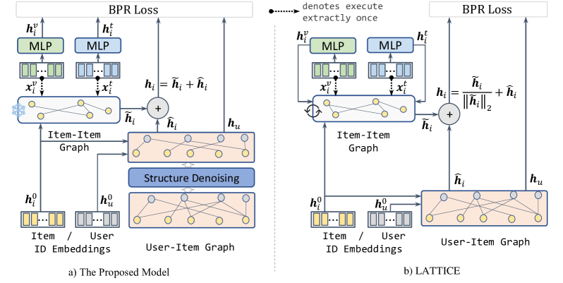
Figure 1. Comparison of our proposed a) FREEDOM and b) LATTICE (Zhang et al., 2021). FREEDOM freezes the item-item graph and denoises the user-item graph simultaneously for multimodal recommendation.

3. Freezing and Denoising Graph Structures

In this section, we elaborate on each component of FREEDOM from graph construction to item recommendation. Fig. 1 shows the overall architecture compared with LATTICE.

3.1. Constructing Frozen Item-Item Graph

Following (Zhang et al., 2021), FREEDOM also uses $k$NN to construct an initial modality-aware item-item graph $\bm{S}^{m}$ using raw features from each modality $m$. Considering $N$ items, we calculate the similarity score $\bm{S}^{m}_{ij}$ between item pair $i$ and $j$ with a cosine similarity function on their raw features ($\bm{x}_{i}^{m}$ and $\bm{x}_{j}^{m}$) of modality $m$. That is:

(1) $$\bm{S}_{ij}^{m}=\frac{{(\bm{x}_{i}^{m})}^{\top}\bm{x}_{j}^{m}}{\|\bm{x}_{i}^{m}\|\|\bm{x}_{j}^{m}\|},$$

where $\bm{S}^{m}_{ij}$ is the $i$-th row, $j$-th column element of matrix $\bm{S}^{m}\in\mathbb{R}^{N\times N}$. We further employ $k$NN sparsification (Chen et al., 2009) and convert the weighted $\bm{S}^{m}$ into an unweighted matrix. That is, for each item $i$, we only retain the connection relations of its top-$k$ similar edges:

(2) $$\widehat{\bm{S}}^{m}_{ij}=\begin{cases}1,\enspace&{\bm{S}}^{m}_{ij}\in\operatorname{top-}k({\bm{S}}^{m}_{i}),\\ 0,\enspace&\text{otherwise}.\end{cases}$$

Each element in $\widehat{\bm{S}}^{m}$ is either 0 or 1, with 1 denoting a latent connection between the two items. We empirically fixed the value of $k$ at 10. Note that $\widehat{\bm{S}}^{m}$ is different from the weighted similarity matrix of LATTICE, which uses the affinity values between items as its elements. We normalize the discretized adjacency matrix $\widehat{\bm{S}}^{m}$ as $\widetilde{\bm{S}}^{m}=({\bm{D}^{m}})^{-\frac{1}{2}}\widehat{\bm{S}}^{m}({\bm{D}^{m}})^{-\frac{1}{2}}$, where $\bm{D}^{m}\in\mathbb{R}^{N\times N}$ is the diagonal degree matrix of $\widehat{\bm{S}}^{m}$ and $\bm{D}_{ii}^{m}=\sum_{j}\widehat{\bm{S}}^{m}_{ij}$. With the resulted modality-aware adjacency matrices, we construct the latent item-item graph by aggregating the structures from each modality:

(3) $${\bm{S}}=\sum_{m\in\mathcal{M}}\alpha_{m}\widetilde{\bm{S}}^{m},$$

where $\bm{S}\in\mathbb{R}^{N\times N}$, $\alpha_{m}$ is the importance score of modality $m$ and $\mathcal{M}$ is the set of modalities. Same as other studies (Liu et al., 2019; Zhang et al., 2021), we consider visual and textual modalities denoted by $\mathcal{M}=\{v,t\}$ in this paper. The importance score can be learned via parametric functions. Here, we reduce the model parameters by introducing a hyperparameter $\alpha_{v}$ denoting the importance of visual modality in constructing $\bm{S}$. We let $\alpha_{t}=1-\alpha_{v}$.

Finally, we freeze the latent item-item graph, which can greatly improve the efficiency of FREEDOM. To be specific, the construction of the similarity matrix under modality $m$ in Eq. (1) requires computational complexity of $\mathcal{O}(N^{2}d_{m})$, where $d_{m}$ is the dimension of raw features. As shown in Fig. 1, FREEDOM pre-calculates (dotted lines) the item-item graph before training and freezes it during model training. As a result, it removes the computational burden of $\mathcal{O}(N^{2}d_{m})$ for graph construction in training.

3.2. Denoising User-Item Bipartite Graph

In this section, we introduce a degree-sensitive edge pruning to denoise the user-item bipartite graph. The idea is derived from recent researches on model sparsification (Rong et al., 2020) and simplification (Chen et al., 2020). Specifically, DropEdge (Rong et al., 2020) randomly drops a certain ratio of edges in training. In (Chen et al., 2020), the authors verify that popular nodes are more likely to suffer from over-smoothing. Inspired by the finding, we sparsify the graph by pruning superfluous edges following a degree-sensitive probability.

Formally, we denote a user-item graph as $\mathcal{G}=(\mathcal{V},\mathcal{E})$, where $\mathcal{V}$ is the set of nodes and $\mathcal{E}$ is the set of edges. The number of users and items in the user-item graph is $M$ and $N$, respectively. We have $M+N=|\mathcal{V}|$, where $|\cdot|$ denotes the cardinality of a set. We construct a symmetric adjacency matrix $\bm{A}\in\mathbb{R}^{|\mathcal{V}|\times|\mathcal{V}|}$ from the user-item interaction matrix $\bm{R}\in\mathbb{R}^{M\times N}$:

(4) $$\bm{A}=\begin{pmatrix}\bm{0}&\bm{R}\\ \bm{R}^{\top}&\bm{0}\end{pmatrix},$$

and each entry $\bm{A}_{ui}$ of $\bm{A}$ is set to 1, if user $u$ has interacted with item $i$, otherwise, $\bm{A}_{ui}$ is set to 0.

Given a specific edge $e_{k}\in\mathcal{E},(0\leq k<|\mathcal{E}|)$ which connects node $i$ and $j$, we calculate its probability as $p_{k}=\frac{1}{\sqrt{\omega_{i}}\sqrt{\omega_{j}}}$, where $\omega_{i}$ and $\omega_{j}$ are the degrees of nodes $i$ and $j$ in graph $\mathcal{G}$, respectively. Usually, we prune a certain proportion $\rho$ of edges of the graph. That is, the number of edges should be pruned is $\lfloor\rho|\mathcal{E}|\rfloor$, where $\lfloor\cdot\rfloor$ is the floor function. As a result, the number of retained edges is $n=\lceil|\mathcal{E}|(1-\rho)\rceil$. Thus, we sample edges from the multinomial distribution with index $n$ and parameter vector $\bm{p}=\langle p_{0},p_{1},\cdots,p_{|\mathcal{E}|-1}\rangle$. In this way, edges connecting high-degree nodes have a low probability to be sampled from the graph. That is, these edges are more likely to be pruned in $\mathcal{G}$. We then construct a symmetric adjacency matrix $\bm{A}_{\rho}$ based on the sampled edges following Eq. (4). In line with prior latent item-item graph, we also perform the re-normalization trick on $\bm{A}_{\rho}$, resulting as $\widehat{\bm{A}}_{\rho}$. Same as DropEdge, FREEDOM prunes the user-item graph and normalizes the sampled adjacency matrix iteratively in each training epoch. However, we resort to the original normalized adjacency matrix $\widehat{\bm{A}}=\bm{D}^{-1/2}\bm{A}\bm{D}^{-1/2}$ in model inference.

3.3. Integration of Two Graphs for Learning

We perform graph convolutions on both graphs, that is, we employ a light-weighted GCN (He et al., 2020) for information propagation and aggregation on $\bm{S}$ and $\widehat{\bm{A}}_{\rho}$. Specifically, the graph convolution over the item-item graph is defined as:

(5) $$\widetilde{\bm{h}}_{i}^{l}=\sum_{j\in\mathcal{N}(i)}{\bm{S}}_{ij}\widetilde{\bm{h}}_{j}^{l-1},$$

where $\mathcal{N}(i)$ is the neighbor items of $i$, $\widetilde{\bm{h}}_{i}^{l}\in\mathbb{R}^{d}$ is the $l$-th layer item representation of item $i$, $\widetilde{\bm{h}}_{i}^{0}$ denotes its corresponding ID embedding vector and $d$ is the dimension of an item or user ID embedding. We stack $L_{ii}$ convolutional layers on the item-item graph $\bm{S}$ and obtain the last layer representation $\widetilde{\bm{h}}_{i}^{L_{ii}}$ as the representation $\widetilde{\bm{h}}_{i}\in\mathbb{R}^{d}$ of $i$ from the multimodal view:

(6) $$\widetilde{\bm{h}}_{i}=\widetilde{\bm{h}}_{i}^{L_{ii}}.$$

Analogously, in the user-item graph, we perform $L_{ui}$ convolutional operations on $\widehat{\bm{A}}_{\rho}$ and obtain embedding of a user $\widehat{\bm{h}}_{u}\in\mathbb{R}^{d}$ or an item $\widehat{\bm{h}}_{i}\in\mathbb{R}^{d}$ with a readout function on all the hidden representations resulted in each layer:

(7) $$\begin{split}\widehat{\bm{h}}_{u}&=\operatorname{READOUT}(\widehat{\bm{h}}_{u}^{0},\widehat{\bm{h}}_{u}^{1},\cdots,\widehat{\bm{h}}_{u}^{L_{ui}}),\\ \widehat{\bm{h}}_{i}&=\operatorname{READOUT}(\widehat{\bm{h}}_{i}^{0},\widehat{\bm{h}}_{i}^{1},\cdots,\widehat{\bm{h}}_{i}^{L_{ui}}),\end{split}$$

where the $\operatorname{READOUT}$ function can be any differentiable function, $\widehat{\bm{h}}_{u}^{0}$ and $\widehat{\bm{h}}_{i}^{0}=\widetilde{\bm{h}}_{i}^{0}$ denotes the ID embeddings of user $u$ and item $i$, respectively. We use the default mean function of LightGCN (He et al., 2020) for embedding readout.

Finally, we use the user representation output by the user-item graph as its final representation. For the item, we sum up the representations obtained from the two graphs as its final representation.

(8) $$\begin{split}{\bm{h}_{u}}&=\widehat{\bm{h}}_{u},\\ {\bm{h}_{i}}&=\widetilde{\bm{h}}_{i}+\widehat{\bm{h}}_{i}.\end{split}$$

To fully explore the raw features, we project multimodal features of item $i$ in each modality via MLPs.

(9) $$\bm{h}_{i}^{m}=\bm{x}_{i}^{m}\bm{W}_{m}+\bm{b}_{m},$$

where $\bm{W}_{m}\in\mathbb{R}^{d_{m}\times d},\bm{b}_{m}\in\mathbb{R}^{d}$ denote the linear transformation matrix and bias in the MLP. In this way, each uni-modal representation $\bm{h}_{i}^{m}$ shares the same latent space with its ID embedding $\bm{h}_{i}$.

For model optimization, we adopt the pairwise Bayesian personalized ranking (BPR) loss (Rendle et al., 2009), which encourages the prediction of a positive user-item pair to be scored higher than its negative pair:

$$\mathcal{L}_{bpr}=\sum_{(u,i,j)\in\mathcal{D}}\Bigl{(} -\operatorname{log}\sigma(\bm{h}_{u}^{\top}\bm{h}_{i}-\bm{h}_{u}^{\top}\bm{h}_{j})+$$

(10) $$\lambda\sum_{m\in\mathcal{M}}-\operatorname{log}\sigma(\bm{h}_{u}^{\top}\bm{h}_{i}^{m}-\bm{h}_{u}^{\top}\bm{h}_{j}^{m})\Bigr{)},$$

where $\mathcal{D}$ is the set of training instances, and each triple $(u,i,j)$ satisfies $\bm{A}_{ui}=1~{}\text{and}~{}\bm{A}_{uj}=0$. $\sigma(\cdot)$ is the sigmoid function and $\lambda$ is a hyperparameter of FREEDOM to weigh the reconstruction losses between user-item ID embeddings and projected multimodal features.

3.4. Top-$K$ Recommendation

To generate item recommendations for a user, we first predict the interaction scores between the user and candidate items. Then, we rank candidate items based on the predicted interaction scores in descending order, and choose $K$ top-ranked items as recommendations to the user. The interaction score is calculated as:

(11) $$r(\bm{h}_{u},\bm{h}_{i})=\bm{h}_{u}^{\top}\bm{h}_{i}.$$

A high score suggests that the user prefers the item. Note that we only use user and item ID embeddings for prediction, because we empirically find the adding of projected item multimodal features in prediction does not show improvement on performance. However, the item multimodal representations can partially benefit the learning of user representations in FREEDOM via Eq. (10).

4. Spectral Analysis

In this section, we examine the benefits of freezing the item-item graph in FREEDOM through the lens of spectral analysis. We show that it possesses a tighter upper bound on the graph spectrum. In addition, we empirically calculate the largest eigenvalues of the normalized graph Laplacian on experimental datasets to validate our analysis.

4.1. Preliminaries

Without loss of generality, we analyze the normalized item-item adjacency matrix $\widetilde{\bm{S}}^{m}=({\bm{D}^{m}})^{-\frac{1}{2}}\widehat{\bm{S}}^{m}({\bm{D}^{m}})^{-\frac{1}{2}}$ within a specific modality $m$. We denote the corresponding matrix of LATTICE as $\widetilde{\bm{S}^{\prime}}^{m}=({\bm{D}^{\prime m}})^{-\frac{1}{2}}\widehat{\bm{S}^{\prime}}^{m}({\bm{D}^{\prime m}})^{-\frac{1}{2}}$. We omit $m$ for clarity in the following analysis.

4.2. Theoretical Analysis

Lemma 4.1.

The eigenvalues of the frozen matrix in FREEDOM possess a tighter upper bound.

Proof.

Let $\lambda$ be an eigenvalue of the non-negative matrix $\widetilde{\bm{S}}$.

$$\widetilde{\bm{S}}\bm{x}=\lambda\bm{x} \Longrightarrow\lambda\left|x_{i}\right|=\left|\sum_{j=1}^{n}\tilde{s}_{ij}x_{j}\right|\leq\left(\sum_{j=1}^{n}\tilde{s}_{ij}\right)\max_{j}\left|x_{j}\right|$$

$$\Longrightarrow\lambda\max_{i}\left|x_{i}\right|\leq\max_{i}\left(\sum_{j=1}^{n}\tilde{s}_{ij}\right)\max_{j}\left|x_{j}\right|$$

(12) $$\Longrightarrow\lambda\leq\max_{i}\left(\sum_{j=1}^{n}\tilde{s}_{ij}\right)\leq n\max_{i,j}\tilde{s}_{ij}$$

Each element in $\widetilde{\bm{S}}$ of FREEDOM and $\widetilde{\bm{S}^{\prime}}$ of LATTICE is positive, with the form of $\tilde{s}_{ij}/\sqrt{d_{ii}d_{jj}}$ and $\tilde{s^{\prime}}_{ij}/\sqrt{d^{\prime}_{ii}d^{\prime}_{jj}}$. As function $g(\tilde{s^{\prime}}_{ij})=\tilde{s^{\prime}}_{ij}/(\tilde{s^{\prime}}_{ij}+\sum_{k\neq i}\tilde{s^{\prime}}_{kj})$ is monotonically increasing, and maximizing Eq. (12) requires the maximized $\tilde{s^{\prime}}_{ij}\geq\bar{d_{ii}}$ (average value of node degree). Hence, we can derive $\max_{i,j}\tilde{s}_{ij}\leq\max_{i,j}\tilde{s^{\prime}}_{ij}$. ∎

In consideration of the page limit, we have moved the more detailed proof to Appendix A. Readers can access it for a more comprehensive understanding of our work.

Table 2. Comparison of the largest eigenvalues of FREEDOM and LATTICE on different datasets (lower is better).

Model	Baby	Sports	Clothing
FREEDOM	1.1685	1.1016	1.0932
LATTICE	1.1796	1.1180	1.1210

4.3. Empirical Study

We compute the largest eigenvalues of the item-item matrix in both FREEDOM and LATTICE, as shown in Table 2. The results validate our previous analysis. A tighter upper bound of eigenvalues in the item-item graph ensures that the frozen item-item graph in FREEDOM can act as a low-pass filter, eliminating the effect of negative coefficients at large frequencies. We further investigate the impact of the frozen item-item graph in FREEDOM and the learnable graph in LATTICE on validation accuracy. The plots in Fig. 2 reveal that graphs in FREEDOM trained with this property achieve higher accuracy and more stable performance than LATTICE.

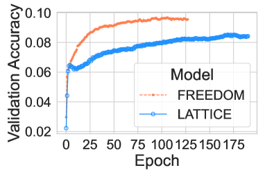
(a)

(b)

Figure 2. Validation accuracy (i.e., Recall@20) of FREEDOM and LATTICE using frozen and learnable item-item matrices, respectively.

5. Experiments

To evaluate the effectiveness and efficiency of our proposed FREEDOM, we conduct experiments to answer the following research questions on three real-world datasets.

• RQ1: How does FREEDOM perform compared with the state-of-the-art methods for recommendation? As our model improves LATTICE (Zhang et al., 2021) by freezing and denoising the graph structures, how about its improvement over LATTICE?

• RQ2: How efficient of our proposed FREEDOM in terms of computational complexity and memory cost?

• RQ3: How do different components in FREEDOM influence its recommendation accuracy?

• RQ4: How sensitive is our model under the perturbation of hyperparameters?

Table 3. Statistics of the experimental datasets.

Dataset	# Users	# Items	# Interactions	Sparsity
Baby	19,445	7,050	160,792	99.88%
Sports	35,598	18,357	296,337	99.95%
Clothing	39,387	23,033	278,677	99.97%

5.1. Experimental Datasets

Following (Zhang et al., 2021), we conduct experiments on three categories of the Amazon review dataset (He and McAuley, 2016a): (a) Baby, (b) Sports and Outdoors, and (c) Clothing, Shoes and Jewelry. For simplicity, we denote them as Baby, Sports and Clothing, respectively. The Amazon review dataset provides both visual and textual information about the items and varies in the number of items under different categories. The raw data of each dataset are pre-processed with a 5-core setting on both items and users, and their filtered results are presented in Table 3. We directly use the 4,096-dimensional visual features extracted by pre-trained Convolutional Neural Networks (He and McAuley, 2016a). For the textual modality, we extract a 384-dimensional textual embedding by utilizing sentence-transformers (Reimers and Gurevych, 2019)  on the concatenation of the title, descriptions, categories, and brand of each item.

5.2. Baseline Methods

To demonstrate the effectiveness of FREEDOM, we compare it with the state-of-the-art recommendation methods in two categories.

First category comprises two general CF models that recommend personalized items to users solely based on user-item interactions:

• BPR (Rendle et al., 2009) optimizes the latent representations of users and items under the framework of matrix factorization (MF) with a BPR loss.

• LightGCN (He et al., 2020) simplifies the vanilla GCN by removing its non-linear activation and feature transformation layers for recommendation.

While the second line of work includes six multimodal recommendation models that leverage both user interactions and multimodal information about items for recommendation:

• VBPR (He and McAuley, 2016b) incorporates visual features for user preference learning under the MF framework and BPR loss. Following (Zhang et al., 2021; Wang et al., 2021b), we concatenate the multimodal features of an item as its visual feature for user preference learning.

• MMGCN (Wei et al., 2019) fuses the representations generated by GCNs in each modality of items for recommendation.

• GRCN (Wei et al., 2020) refines the user-item bipartite graph with the removal of false-positive edges for multimodal recommendation. Based on the refined graph, it then learns user and item representations by performing information propagation and aggregation via GCNs.

• DualGNN (Wang et al., 2021b) augments the representations of users in GCNs with an additional user-user correlation graph that is extracted from the user-item graph.

• LATTICE (Zhang et al., 2021) learns the latent semantic item-item structures from the multimodal features for recommendation. As FREEDOM improves LATTICE, we highlight its improvement over LATTICE in Table 4.

• SLMRec (Tao et al., 2022) incorporates self-supervised learning into multimedia recommendation. It proposes three data augmentations to uncover the multimodal patterns in data for contrastive learning.

5.3. Evaluation Protocols

For a fair comparison, we adopt the same evaluation settings of (Wang et al., 2021b; Zhang et al., 2021; Tao et al., 2022). Specifically, we use two widely-used evaluation protocols for top-$K$ recommendation: Recall@$K$ and NDCG@$K$, which we refer to as R@$K$ and N@$K$ in brief. We report the average metrics of all users in the test set under both $K=10$ and $K=20$. For each user in the evaluated dataset, we randomly split 80% of historical interactions for training, 10% for validation and the remaining 10% for testing. During training, we conduct the negative sampling strategy to pair each observed user-item interaction in the training set with one negative item that the user does not interact with before. We use the all-ranking protocol to compute the evaluation metrics for recommendation accuracy comparison.

5.4. Implementation and Hyperparameter Settings

Following existing work (He et al., 2020; Zhang et al., 2021), we fix the embedding size of both users and items to 64 for all models, initialize the embedding parameters with the Xavier method (Glorot and Bengio, 2010), and use Adam (Kingma and Ba, 2015) as the optimizer. For a fair comparison, we carefully tune the parameters of each model following their published papers. All models are implemented by PyTorch (Paszke et al., 2019) and evaluated on a Tesla V100 GPU card with 32 GB memory. To reduce the hyperparameters searching space of FREEDOM, we fix the number of GCN layers in the user-item bipartite graph and the item-item graph at $L_{ui}=2$ and $L_{ii}=1$, respectively. We empirically fix the hyperparameter of $\lambda$ at $1e-03$ and the visual feature ratio $\alpha_{v}$ at 0.1. We then perform a grid search on other hyperparameters of FREEDOM across all datasets to conform to its optimal settings. Specifically, the ratio $\rho$ of the degree-sensitive edge pruning is searched from {0.8, 0.9}. For convergence consideration, the early stopping and total epochs are fixed at 20 and 1000, respectively. Following (Zhang et al., 2021), we use R@20 on the validation data as the training stopping indicator. To ensure a fair comparison, all baseline models as well as our proposed model have been integrated into the unified multimodal recommendation framework, MMRec (Zhou, 2023).

Table 4. Overall performance achieved by different recommendation methods in terms of Recall and NDCG. We mark the global best results on each dataset under each metric in boldface and the second best is underlined. Improvement percentage (improv.) is calculated as the ratio of performance increment from LATTICE to FREEDOM under each dataset and metric. To verify the stability of our method, we conduct experiments across 5 different seeds and state the improvements are statistically significant at the level of $p$ ¡ 0.01 with a paired $t$-test.

Dataset	Metric	General CF model		Multimodal model
		BPR	LightGCN	VBPR	MMGCN	GRCN	DualGNN	SLMRec	LATTICE	FREEDOM	improv.
Baby	R@10	0.0357	0.0479	0.0423	0.0421	0.0532	0.0513	0.0521	0.0547	0.0627	14.63%
	R@20	0.0575	0.0754	0.0663	0.0660	0.0824	0.0803	0.0772	0.0850	0.0992	16.71%
	N@10	0.0192	0.0257	0.0223	0.0220	0.0282	0.0278	0.0289	0.0292	0.0330	13.01%
	N@20	0.0249	0.0328	0.0284	0.0282	0.0358	0.0352	0.0354	0.0370	0.0424	14.59%
Sports	R@10	0.0432	0.0569	0.0558	0.0401	0.0599	0.0588	0.0663	0.0620	0.0717	15.65%
	R@20	0.0653	0.0864	0.0856	0.0636	0.0919	0.0899	0.0990	0.0953	0.1089	14.27%
	N@10	0.0241	0.0311	0.0307	0.0209	0.0330	0.0324	0.0365	0.0335	0.0385	14.93%
	N@20	0.0298	0.0387	0.0384	0.0270	0.0413	0.0404	0.0450	0.0421	0.0481	14.25%
Clothing	R@10	0.0206	0.0361	0.0281	0.0227	0.0421	0.0452	0.0442	0.0492	0.0629	27.85%
	R@20	0.0303	0.0544	0.0415	0.0361	0.0657	0.0675	0.0659	0.0733	0.0941	28.38%
	N@10	0.0114	0.0197	0.0158	0.0120	0.0224	0.0242	0.0241	0.0268	0.0341	27.24%
	N@20	0.0138	0.0243	0.0192	0.0154	0.0284	0.0298	0.0296	0.0330	0.0420	27.27%

5.5. Performance Comparison

Effectiveness (RQ1)

Table 4 reports the comparison of recommendation accuracy in terms of Recall and NDCG, from which we have the following observations: 1). Although LATTICE obtains the second best results on Baby and Clothing datasets, FREEDOM improves LATTICE by an average of 19.07% across all datasets and outperforms other baselines as well. The improvements attribute to the graph structures denoising and freezing components of FREEDOM. Denoising the user-item graph in $\bm{A}$ reduces the impact of noise signal in false-positive interactions. The frozen item-item graph in FREEDOM ensures the items are relevant to each other if linked because it built on the raw multimodal features. On the contrary, the latent item-item graph is dynamically learned via projecting the raw multimodal features into a low-dimensional space. The affinity of two items in the graph depends on not only the raw multimodal features but also the projectors (i.e., MLPs). 2). Generally, both general MF (i.e., BPR) and graph-based (i.e., LightGCN) models can benefit from the multimodal information. For example, VBPR leveraging multimodal features outperforms BPR by up to 27.63% on average. Most graph-based multimodal models except MMGCN show better recommendation results than MF models (i.e., BPR and VBPR) and general CF models. However, we observe that the performance of MMGCN is inferior to that of BPR on Sports dataset. One potential reason for this might be that the textual and visual representations extracted from the texts and images of products in the Sports dataset are less informative than those of the Baby and Clothing datasets. Another reason may be the fusion mechanism used in MMGCN, which sums up the features from all modalities, making it difficult to discern the prominent contribution of individual modalities. Our proposed FREEDOM utilizing LightGCN as its backbone network gains a significant margin of 42.79% over the original LightGCN on average. 3). In graph-based multimodal models, compared with MMGCN, GRCN utilizes simplified graph convolutional operations and refines the user-item bipartite graph by assigning weights based on the affinities of user preferences and item contents. It shows better performance in dense datasets, but is inferior in Clothing dataset. The reason is that the assignments of low weights on less similar user-item edges impede the information propagation of GCNs in a sparse dataset. DualGNN and SLMRec utilize auxiliary information to augment the representation learnings on users and items. They have comparable performance with each other on the evaluated dataset except Sports. One potential reason is that the extracted textual and visual representations from the texts and images of products in Sports are less informative than that of Baby and Clothing datasets. The evidence is that in Table 4, the improvements achieved by GRCN and DualGNN over LightGCN in Sports are not as significant as that of Baby and Clothing. SLMRec augments the representation from each modality of an item with self-supervised learning and gains better results than GRCN and DualGNN in Sports. Analogously, both LATTICE and FREEDOM augment the representations of items via a latent item-item graph and show competitive results.

Overall, the experiment results in Table 4 validate the effectiveness of augmenting item representation with multimodal information. Furthermore, freezing the latent graph structure of the item as in FREEDOM can help achieve even better performance.

Efficiency (RQ2)

We report the memory and training time consumed by FREEDOM and baselines in Table 5. From the table, we observe: 1). Multimodal models usually utilize more memory than the general CF models as they need to process modality-aware features. Graph-based models perform convolutional operations on graphs and cost more time on training. DualGNN consumes even more time in training because the convolutional operations are performed not only on the user-item graph but also on the user-user relationship graph. MMGCN propagates convolutional operators on each modality, resulting in increased training time. 2). Compared FREEDOM with LATTICE, the proposed FREEDOM can reduce the memory cost and training time of LATTICE on Clothing by 6$\times$ and 4$\times$, respectively. FREEDOM removes the construction of latent item-item graph in each training epoch, it pre-builds the graph before training and freezes it during training. With the removal of item-item graph construction in training, FREEDOM is preferable with large graphs.

Table 5. Comparison of FREEDOM against state-of-the-art baselines on model efficiency.

Dataset	Metric	General CF model		Multimodal model
		BPR	LightGCN	VBPR	MMGCN	GRCN	DualGNN	SLMRec	LATTICE	FREEDOM
Baby	Memory (GB)	1.59	1.69	1.89	2.69	2.95	2.05	2.08	4.53	2.13
	Time ($s$/epoch)	0.47	0.99	0.57	3.48	2.36	7.81	1.91	1.61	1.25
Sports	Memory (GB)	2.00	2.24	2.71	3.91	4.49	2.81	3.04	19.93	3.34
	Time ($s$/epoch)	0.95	2.86	1.28	16.60	6.74	12.60	5.52	10.71	3.46
Clothing	Memory (GB)	2.16	2.43	3.02	4.24	4.58	3.02	3.40	28.22	4.15
	Time ($s$/epoch)	0.97	2.94	1.29	16.71	7.21	13.44	5.09	15.96	3.67

5.6. Ablation Study (RQ3)

In this section, we decouple the proposed FREEDOM and evaluate the contribution of each component with regard to recommendation accuracy. We design the following variants of FREEDOM based on its architecture:

• FREEDOM-D denoises the user-item graph in FREEDOM without freezing the item-item graph.

• FREEDOM-F improves LATTICE merely by the freezing component of FREEDOM, which freezes the item-item graph as introduced in Section 3.

• FREEDOM-R replaces the denoising method of degree-sensitive edge pruning in FREEDOM with random edge dropout (Rong et al., 2020).

• FREEDOM-0 ablates the contribution of multimodal losses in Eq. (10) by setting $\lambda$ to 0.

We report the comparison results in terms of R@20 and N@20 with Fig. 4. The results show that the freezing component of FREEDOM attributes significantly to its overall performance. However, denoising the user-item graph can further improve the performance. Freezing the item-item graph in FREEDOM (i.e., FREEDOM-F) gains consistent improvements over LATTICE on three datasets, but not for the denoising component. We speculate that without the freezing component, the denoising component may affect graph connectivity on sparse graphs and result in performance degradation. FREEDOM-R with random edge dropout shows slight improvement over FREEDOM-F but is still worse than FREEDOM, showing the effectiveness of degree-sensitive edge pruning. The performance of FREEDOM-0 is comparable to FREEDOM, indicating the effective design of FREEDOM in freezing and denoising graph structures for recommendation. However, FREEDOM can benefit slightly from the inclusion of multimodal losses.

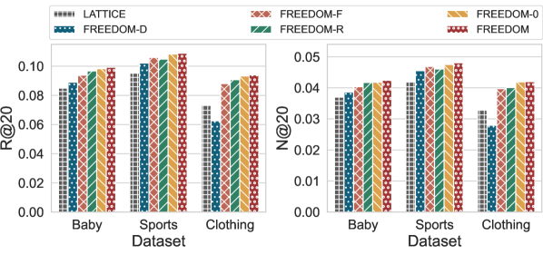
Figure 3. Comparison of LATTICE with FREEDOM variants.

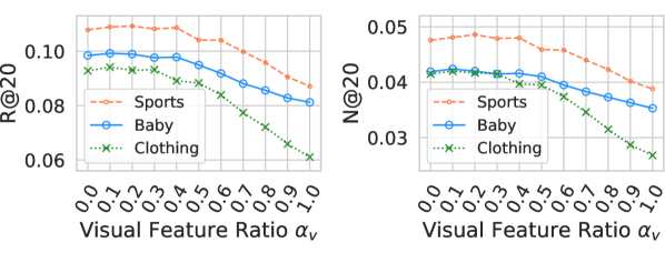
Figure 4. Performance of FREEDOM changes with the ratio of visual features in constructing the item-item graph.

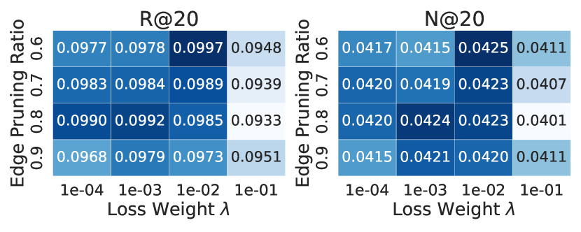
(a) Baby

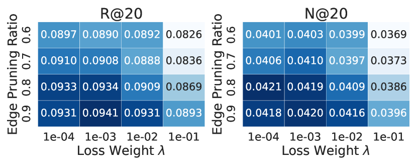
(b) Clothing

Figure 5. Performance of FREEDOM with regard to different loss weights $\lambda$ and edge pruning ratios $\rho$ on Baby and Clothing datasets.

5.7. Hyperparameter Sensitivity Study (RQ4)

Multimodal Features. FREEDOM uses the raw textual and visual features extracted from pre-trained models to construct the latent item-item graph. We first study how information from different modalities could affect the performance of FREEDOM by adjusting the ratio of visual features from 0.0 to 1.0 with a step of 0.1 in constructing the graph. A ratio of 0.0 on visual features means that the construction of item-item graph depends only on textual features. The item-item graph, on the other hand, is based on visual features if the ratio is 1.0. The recommendation results on R@20 and N@20 for three evaluated datasets are shown in Fig. 4. From the results, we may infer that the textual features are more informative than the visual features in constructing an effective item-item graph.

The Dropout Ratio and Loss Weight. We vary the edge pruning ratio $\rho$ in the denoising component of FREEDOM from 0.6 to 0.9 with a step of 0.1, and vary the loss weight $\lambda$ in {1e-04, 1e-03, 1e-02, 1e-01}. Fig. 5(a) and 5(b) show the performance achieved by FREEDOM under different combinations of embedding dropout ratios and weights on Baby and Clothing, respectively. The results suggest a high edge pruning ratio of FREEDOM on large graphs. Compared with the edge pruning ratio, the performance of FREEDOM is less sensitive to the settings of loss trade-off $\lambda$. However, placing a high weight on multimodal loss might limit the expressive power of FREEDOM and results in performance degradation.

6. Conclusion

In this paper, we experimentally reveal that the graph structure learning in a state-of-the-art multimodal recommendation model (i.e., LATTICE (Zhang et al., 2021)) plays a trivial role in its performance. It is the item-item graph constructed from raw multimodal features that contributes to the recommendation accuracy. Based on the finding, we propose a model that freezes the item-item graph and denoises the user-item graph simultaneously for multimodal recommendation. Through both theoretical and empirical analysis, we demonstrate that freezing the item-item graph in FREEDOM can yield various benefits. In denoising, we devise a degree-sensitive edge pruning method to sample the user-item graph, which shows better performance than the random edge dropout (Rong et al., 2020) for recommendation. Finally, we conduct extensive experiments to demonstrate the effectiveness and efficiency of FREEDOM in multimodal recommendation.

Appendix A Proof of LEMMA 4.1

Let $s^{\prime}_{ij}$ represent the element in the adjacency matrix of LATTICE and let $s_{ij}$ represent the corresponding element in FREEDOM. We can derive that $s_{ij}=1\geq s^{\prime}_{ij}$. As defined in the paper, $\bm{D}^{\prime}=\mathrm{diag}(d^{\prime}_{11},\cdots,d^{\prime}_{nn})$ is a diagonal matrix where each entry on the diagonal is equal to the row-sum of the adjacency matrix $d^{\prime}_{ii}=\sum_{j}s^{\prime}_{ij}$. The normalized adjacency matrix $\widetilde{\bm{S}^{\prime}}$ in LATTICE can be denoted as follows:

$$\widetilde{\bm{S}^{\prime}}=\begin{bmatrix}1/d^{\prime}_{11}&{s^{\prime}}_{12}/\sqrt{d^{\prime}_{11}d^{\prime}_{22}}&\dots&{s^{\prime}}_{1n}/\sqrt{d^{\prime}_{11}d^{\prime}_{nn}}\\ {s^{\prime}}_{21}/\sqrt{d^{\prime}_{22}d^{\prime}_{11}}&1/d^{\prime}_{22}&\dots&{s^{\prime}}_{2n}/\sqrt{d^{\prime}_{22}d^{\prime}_{nn}}\\ \vdots&\vdots&&\vdots\\ {s^{\prime}}_{n1}/\sqrt{d^{\prime}_{nn}d^{\prime}_{11}}&{s^{\prime}}_{n2}/\sqrt{d^{\prime}_{nn}d^{\prime}_{22}}&\dots&1/d^{\prime}_{nn}\end{bmatrix}$$

Analogously, we can derive the normalized adjacency matrix in FREEDOM. We denote the elements in the normalized adjacency matrices of $\widetilde{\bm{S^{\prime}}}$ and $\widetilde{\bm{S}}$ as $\tilde{s^{\prime}}_{ij}$ and $\tilde{s}_{ij}$, respectively. As stated in the paper, the function $g(\tilde{s^{\prime}}_{ij})=\tilde{s^{\prime}}_{ij}/(\tilde{s^{\prime}}_{ij}+\sum_{k\neq i}\tilde{s^{\prime}}_{kj})$ is monotonically increasing. To maximize Eq. (13) in the paper, $\tilde{s^{\prime}}_{ij}$ must also be maximized. From the above equations, we can deduce that the maximum value for either $\widetilde{\bm{S}}$ or $\widetilde{\bm{S^{\prime}}}$ lies on its diagonal. Therefore, we can derive that $max_{i,j}\tilde{s}_{ij}=1/d_{ii}=1/\sum_{j}s_{ij}\leq max_{i,j}\tilde{s^{\prime}}_{ij}=1/d^{\prime}_{ii}=1/\sum_{j}s^{\prime}_{ij}$.