Applications of
the Spectral Theory of Chemical Bonding
to Simple Hydrocarbons

Abstract

The finite-basis, pair formulation of the Spectral Theory of chemical bonding is briefly surveyed. Solutions of the Born-Oppenheimer polyatomic Hamiltonian totally antisymmetric in electron exchange are obtained from diagonalization of an aggregate matrix built up from conventional diatomic solutions to atom-localized problems. A succession of transformations of the bases of the underlying matrices and the unique character of symmetric orthogonalization in producing the archived matrices calculated “once-of-all” in the pairwise-antisymmetrized basis are described. Application is made to molecules containing hydrogens and a single carbon atom. Results in conventional orbital bases are given and compared to experimental and high-level theoretical results. Chemical valence is shown to be respected and subtle angular effects in polyatomic contexts are reproduced. Means of reducing the size of the atomic-state basis and improve the fidelity of the diatomic descriptions for fixed basis size, so as to enable application to larger polyatomic molecules, is outlined along with future initiatives and prospects.

AFRL] Air Force Research Lab., 10 E. Saturn Blvd., Edwards AFB, CA 93524, United States

1 Introduction

That molecules are composed of interacting atoms was an important conceptual touchstone in the development of classical chemistry. From this perspective it is perhaps surprising that most contemporary quantum-chemical methods do not make direct use of this insight but construct molecules from electrons and nucleii, instead. In particular the initial step often involves forming, from a number of localized basis functions, one-electron orbitals delocalized across the entire molecule under a mean-field-type, electron-electron interaction. Subsequent correction of this solution can then be regarded as introducing partial relocalization. Post hoc interpretations of these solutions, often involving a localization-approximating unitary transformation or other mathematical manipulations, can then be used in at attempt to gain insights in terms of atoms and their interactions^{1, 2, 3, 4, 5, 6, 7, 8, 9}. (No effort is made here to completely review this literature, but only to provide a starting point for interested readers.)

This publication describes results of the application of one variety of a class of methods referred to as the Spectral Theory of chemical bonding,^{10, 11, 12, 13, 14, 15, 16, 17, 18, 19} which seeks to directly construct quantum-mechanical descriptions of polyatomic molecules from the characteristics of the constituent atoms, namely their electronic eigenspectrum and the state spectra of interacting pairs. These methods differ from some others with similar motivations (also not an exhaustive citation list)^{20, 21, 22, 23, 24} in specific implementation details.

Principal advantages of the Spectral Theory will be shown to include relief from the need to calculate two-electron integrals over three or four centers and the “once for all” determination of reference diatomic matrices ready for universal application to the pairs in any polyatomic molecule which contains the two atoms. Much effort in this (and subsequent publications) is geared toward overcoming the severe size-scaling which will be shown to be exponentially dependent on the number of atoms in the molecule and polynomially dependent upon the size of the state space used to describe the atoms. The overall motivation for the Spectral Theory of chemical bonding is the possibility of recovering, for an N-atom molecule, a significant portion of the N-excitation CI energy, all from archived data only single-excitation in the atoms and (atom-centered) double-excitation in the diatoms.

It is the purpose of this report to itemize the steps of the pairwise-antisymmetrized form of the Spectral Theory in constructing polyatomic wave functions from atomic states via the mediation of totally antisymmetric treatments of the unique interacting pairs of atoms in the molecule. After a description of the theoretical procedures, as currently deployed, there is an account of some results of the application of the theory to simple paradigmatic hydrocarbons containing a single carbon atom and two means by which the atomic state space might be kept relatively small while retaining accuracy.

2 Theoretical methods

2.1 Summary of theoretical/computational development

Much of this discussion follows the progress and notation of ref. 17, especially sections 2 and 3, but focuses on the current flow and set of options to distinguish them from the greater number of possibilities described in previous publications. In addition a few new approaches or deviations from what are described there are explained in more detail. The overall organization is motivated by a “building up” from the more conventional quantum-chemical components toward the more unique aspects of the Spectral Theory. A brief outline of the steps is given in Figure 1 for reference.

Figure 1: Outline of the steps of the finite-basis, pairwise-antisymmetrized form of the Spectral Theory

The overall goal of this section is to justify the construction of solutions of the polyatomic Born-Oppenheimer, quantum-chemical Hamiltonian which are totally antisymmetric in electron exchange and built from finite-basis treatments of all the molecular pairs. These diatomic basis components are themselves totally antisymmetric products of atomic states. Previous publications have referred to this as the “pairwise-antisymmetrized, finite-subspace representation.”

The Spectral Theory development starts from a type of valence-bond theory especially amenable to localized, in this case atomic-centered, calculations. Sometimes referred to as “nonorthogonal valence-bond theory” (NOVB) or “multi-configurational valence bond theory” (MCVB) this configuration-interaction-based approach is implemented in the CRUNCH suite of computational chemistry codes.²⁵ Putting aside implementation details, it can be considered as equivalent to the more common molecular-orbital, configuration-interaction (MOCI) approach but with the additional flexibility that the one-electron orbitals which comprise the configurations need not be orthogonal, but can be strictly localized and even determined by the solution of atomic problems.

2.2 Valence-bond methods for atomic eigensolutions

In the CRUNCH codes configurations for the atomic CI calculations are space-symmetry-adapted constellations of Young standard tableaux^{25, 26, 27} composed of the one-electron orbitals and defined by the NPN spin representation of the symmetric group. These formally spin-free functions in the spatial coordinates $\boldsymbol{i}$ of atom $\alpha$ are labeled $\boldsymbol{\Phi}_{\bf yt}^{(\alpha)}(\boldsymbol{i})$. (In previous Spectral-Theory publications finite-basis matrices and basis functions were notated with a “tilde,” but since only finite-bases are considered here that convention is abandoned.) Because the angular portion of the one-electron functions are complex spherical harmonics, the multi-electron configuration functions each have good spin (S), angular-momentum-projection ($\mathrm{M_{l}}$), and parity (P for g/u) quantum numbers and the configurations can be distinguished by their different orbital occupations. Orbital occupations are chosen such that complete manifolds of $\mathrm{M_{l}}$ functions for each desired atomic L value are spanned.

Strictly, of course, the computations don’t use or express these functions directly, but deliver matrix elements between functions with different orbital occupations and solve matrix equations involving the elements. Because the standard tableau functions (as employed in the current code suite) are not orthonormal, wave functions must be obtained by solution of the generalized-eigenvalue problem.

$${\bf H}_{\bf yt}^{(\alpha)}\cdot{\bf V}_{{\bf H}_{\bf yt}}^{(\alpha)}={\bf S}_{\bf yt}^{(\alpha)}\cdot{\bf V}_{{\bf H}_{\bf yt}}^{(\alpha)}\cdot{\bf E}^{(\alpha)}$$ (1)

${\bf H}_{\bf yt}$ and ${\bf S}_{\bf yt}$ are the Hamiltonian and overlap matrices in the Young Tableau basis ($\bf yt$) and ${\bf E}$ is a diagonal matrix of the eigenvalues. Orthonormal solutions are then obtained from the Young-tableau basis according to:

$$\boldsymbol{\Psi}^{(\alpha)}(\boldsymbol{i})=\boldsymbol{\Phi}_{\bf yt}^{(\alpha)}(\boldsymbol{i})\cdot{\bf V}_{{\bf H}_{\bf yt}}^{(\alpha)}$$ (2)

In addition to the quantum numbers of the configurational basis in which the solution is sought (S, $\mathrm{M_{l}}$, and P), the eigensolutions, because of interactions in the atomic Hamiltonian, manifest additional good quantum numbers. Total orbital angular momentum, L, and an index e which is the order of the energy among solutions with the same values of the other quantum numbers (made unique, as necessary, in the case of accidental degeneracy) are manifested.

2.3 Diatomic solutions in a Young tableau basis

The CRUNCH codes are also used to solve the diatomic problems. The atoms ($\alpha$ and $\beta$) are separated along their quantization axis so the one-electron spatial orbitals can be identical to those used for the atoms but placed separately on each nucleus. Orbitals on different atoms are therefore not orthogonal and neither are constellations of the diatomic Young tableaux which result. The configurations have good quantum numbers associated with the total diatomic spin ($\mathrm{S}_{\alpha\beta}$) and the projection of the total orbital angular momentum along the axis of nuclear separation ($\lambda_{\alpha\beta}^{\prime}$) and can be distinguished or labeled by their orbital occupations. (The “prime” indicates that the quantization axis for angular momentum is different from the global polyatomic quantization axis which will be adopted later.) The CRUNCH codes are capable of forming symmetry-adapted constellations appropriate for homonuclear diatomic molecules in the $D_{\infty h}$ point group. However, because of the transformations described in the next section, the present calculations employ multi-electron configurations only constrained to $C_{\infty v}$. In addition the +/- functions (distinguished by their eigenvalues with respect to reflection through planes containing the internuclear axis) are lumped together as a matter of practice. The sets of orbital occupations are chosen to encompass all combined possibilities of the atomic calculations described in the previous section and so the diatomic treatments are completely size-consistent.

Although not of primary interest to the current investigation, for a diatom ($\alpha,\beta$) with electrons ($\boldsymbol{i}$, $\boldsymbol{j}$), eigenvalues ${\bf E}^{(\alpha,\beta)}(R_{\alpha\beta})$ may be obtained by solving the generalized-eigenvalue problem:

$${\bf H}_{\bf yt}^{(\alpha,\beta)}(R_{\alpha\beta})\cdot{\bf V}_{{\bf H}_{\bf yt}}^{(\alpha,\beta)}(R_{\alpha\beta})={\bf S}_{\bf yt}^{(\alpha,\beta)}(R_{\alpha\beta})\cdot{\bf V}_{{\bf H}_{\bf yt}}^{(\alpha,\beta)}(R_{\alpha\beta})\cdot{\bf E}^{(\alpha,\beta)}(R_{\alpha\beta})$$ (3)

Orthonormal eigenfunctions in the constellation basis are then constructed as:

$$\boldsymbol{\Psi}^{(\alpha,\beta)}(\boldsymbol{i},\boldsymbol{j};R_{\alpha\beta})=\boldsymbol{\Phi}_{\bf yt}^{(\alpha,\beta)}(\boldsymbol{i},\boldsymbol{j})\cdot{\bf V}_{{\bf H}_{\bf yt}}^{(\alpha,\beta)}(R_{\alpha\beta})$$ (4)

The interactions in the diatomic Hamiltonian add parity, P (for g/u (homonuclear)), reflection symmetry, $\sigma$ (for +/-), and an energy index, e, to the good quantum numbers of the CI basis functions already listed.

More directly relevant as the starting point in moving toward the polyatomic Spectral Theory are the Hamiltonian and overlap matrices of eq. 3 in the configuration basis. The linear transformations of this basis which are formulated as transformations of the matrices represented computationally, make up the bulk of the remainder of this section.

Before proceeding, it is perhaps appropriate to discuss in more detail the implications of and to distinguish between what are referred to as “good quantum numbers” and “basis-set labels.” In the context of building up and transforming matrices for the Spectral Theory, and a direct implication of the common usage of this phrase in quantum mechanics, good quantum numbers define Hamiltonian and overlap matrix sub-blocks which, if the underlying subbases are concatenated, have no non-zero matrix elements between them. With proper basis-set order, the supermatrices are block diagonal. Basis set labels are used to definitively identify basis functions, especially with respect to the character of the atomic components of the diatomic functions. Within a matrix block involving states with a common set of quantum numbers there are generally interconnecting non-zero matrix elements between functions with different labels.

2.4 Phase-consistent, atomic-pair basis

The chain of linear transformations of the Spectral Theory begins with modifying the solutions of the atomic problem. The Young-tableaux basis for each atom is transformed to the atomic eigenstate basis of eq. 2. In addition, because of the need to build up polyatomic functions with a phase consistent among the fragments, the arbitrary (with respect to angular-momentum algebra) phase (sign) introduced into ${\bf V}_{{\bf H}_{\bf yt}}^{(\alpha)}$ by the numerical diagonalization of eq. 1 is remedied.

Each of the 2L+1 eigenstates belonging to an L manifold are separately considered. Those with the 2L largest values of $\mathrm{M_{l}}$ are replaced sequentially as follows. Using eq. 2 the eigenfunction with $\mathrm{M_{l}}$ = -L can be written as an expansion of the CI basis functions. Each of its components can then be analytically subjected to orbital- and state- raising operators²⁸ with tableau-rearrangement algorithms allowing re-expression in terms of a linear combination of standard tableaux of unit-increased $\mathrm{M_{l}}$. This new function then replaces the phase-arbitrary initial solution and the process is repeated to phase-rectify the remaining coefficients in each L manifold. Because of the known phase relationship between the one-electron orbitals (preserved in the orbital raising operators), this new manifold of eigensolutions possesses within itself a sign consistency which will ultimately allow the diatomic pair functions to be subjected to a coordinate rotation (eq. 13) which will mix states of differing atomic $\mathrm{M_{l}}$ but the same L (and other quantum numbers). This is possible in spite of the fact that the relative phase between different L manifolds (because of the arbitrary phase between their root, diagonalizer-generated $\mathrm{M_{l}}$ = -L states) remains arbitrary and unknown.

The phase-consistent ($\bf pc$) atomic functions which result can be denoted:

$$\boldsymbol{\Psi}_{\bf pc}^{(\alpha)}(\boldsymbol{i})=\boldsymbol{\Phi}_{\bf yt}^{(\alpha)}(\boldsymbol{i})\cdot{\bf V}_{{\bf H}_{\bf pc}}^{(\alpha)}$$ (5)

In addition to being phase consistent, this set of atomic eigenfunctions retain the good quantum numbers L, $\mathrm{M_{l}}$, S, P, and N of the functions of eq. 2.

The second step involves incorporation of what are referred to as the subduction coefficients^{29, 30, 31}. These allow each diatomic Young tableau, which is totally antisymmetric with respect to electron exchange, to be expressed exactly as a likewise totally antisymmetric linear combination of direct products of atomic Young tableaux. Thus the diatomic basis of eq. 4 can be transformed to an atomic-product basis spanning the same space as:

$$\boldsymbol{\Phi}^{(\alpha\otimes\beta)}(\boldsymbol{i},\boldsymbol{j})=\boldsymbol{\Phi}_{\bf yt}^{(\alpha,\beta)}(\boldsymbol{i},\boldsymbol{j})\cdot{\bf D}_{\bf sub}^{(\alpha,\beta)}$$ (6)

The real matrix ${\bf D}_{\bf sub}^{(\alpha,\beta)}$, independent of atomic separation, includes non-zero coefficients for all spin-couplings between $\mathrm{S}_{\alpha}$ and $\mathrm{S}_{\beta}$ necessary to yield $\mathrm{S}_{\alpha\beta}$ in a common set of orbitals.

Finally combining the coefficients of the phase-consistent atomic eigenstates ${\bf V}_{{\bf H}_{\bf pc}}^{(\alpha)}$ and ${\bf V}_{{\bf H}_{\bf pc}}^{(\beta)}$ with the subduction coefficients ${\bf D}_{\bf sub}^{(\alpha,\beta)}$ into a single orthogonal matrix ${\bf M}_{\bf pc}^{(\alpha,\beta)}$, one obtains the atomic-state pair basis which is referred to in ref. 17 as the valence-bond basis:

$$\boldsymbol{\Phi}_{\bf vb}^{(\alpha,\beta)}(\boldsymbol{i},\boldsymbol{j})\equiv\{\boldsymbol{\Phi}_{\bf pc}^{(\alpha)}(\boldsymbol{i})\otimes\boldsymbol{\Phi}_{\bf pc}^{(\beta)}(\boldsymbol{j})\}=\boldsymbol{\Phi}_{\bf yt}^{(\alpha,\beta)}(\boldsymbol{i},\boldsymbol{j})\cdot{\bf M}_{\bf pc}^{(\alpha,\beta)}$$ (7)

Totally antisymmetric combinations of the phase-consistent atomic eigenstates can thus provide a basis for solution of the diatomic CI problem. The functions in this basis each have good diatomic quantum numbers $\mathrm{S}_{\alpha\beta}$ and $\lambda_{\alpha\beta}^{\prime}$ which are represented collectively by $(\alpha,\beta)$ in the left most symbol. Also implicit in this notation are the basis labels for each of the atomic states of which it is composed ($\mathrm{L}_{\alpha}$, $\mathrm{M}_{\mathrm{l}\alpha}^{\prime}$, $\mathrm{S}_{\alpha}$, $\mathrm{P}_{\alpha}$, $\mathrm{e}_{\alpha}$; $\mathrm{L}_{\beta}$, $\mathrm{M}_{\mathrm{l}\beta}^{\prime}$, $\mathrm{S}_{\beta}$, $\mathrm{P}_{\beta}$, $\mathrm{e}_{\beta}$). In following sections this diatomic basis will be subjected to linear transformations which represent a change in quantum numbers and/or atomic state labels. The more generic representation $(\alpha,\beta)$ will sometimes be replaced by others which emphasize the change in a particular characteristic of the basis. To do so strictly, for every degree of freedom, would excessively proliferate new symbols/superscripts. Nevertheless the good quantum numbers and distinguishing labels of transformed bases will be emphasized in the text accompanying the equations.

Numerically it is the diatomic Hamiltonian and overlap matrices rather than the basis functions, per se, which are subjected to this transformation as, for example:

$${\bf H}_{\bf vb}^{(\alpha,\beta)}(R_{\alpha\beta})={\bf M}_{\bf pc}^{(\alpha,\beta)\,t}\cdot{\bf H}_{\bf yt}^{(\alpha,\beta)}(R_{\alpha\beta})\cdot{\bf M}_{\bf pc}^{(\alpha,\beta)}$$ (8)

For simplicity the diatomic basis has not been notated as being dependent upon internuclear separation. It is in the calculation of matrix elements from the one- and two-electron integrals over functions located on the atoms that the R dependence arises. For convenience, the overlap and Hamiltonian matrices for each separation are now subjected to normalization of the underlying basis.

It is worth noting that as the separation of the atoms approaches infinity, the underlying diatomic basis becomes orthonormal; the overlap matrix becomes the identity and the Hamiltonian matrix becomes diagonal with sums of atomic energies as the only non-zero elements. For finite separations both matrices are generally dense.

It should further be emphasized that this new basis spans the same space as the diatomic Young tableau basis and so it yields precisely the same eigenvalues when these matrices are subjected to diagonalization. The eigenvectors would now be given in the basis of antisymmetric products of atomic eigenstates (c.f. eq. 4).

2.5 Orthogonalized diatomic matrix archive

As is typical in quantum chemistry codes, the CRUNCH suite focuses on calculating the active electronic energy. At this point in the Spectral Theory development (although for simplicity it will not be indicated by a change of the notation) the nuclear repulsion and any frozen-core electronic energy are added back into the Hamiltonian matrices so that they describe total diatomic energies relative to separated electrons and nucleii. In the context of the non-orthogonal basis, this involves replacing ${\bf H}_{\bf vb}^{(\alpha,\beta)}(R_{\alpha\beta})$ with:

$${\bf H}_{\bf vb}^{(\alpha,\beta)}(R_{\alpha\beta})+(E_{\mathrm{nuc}}+E_{\mathrm{core}}){\bf S}_{\bf vb}^{(\alpha,\beta)}(R_{\alpha\beta})$$ (9)

Now for each distance and set of diatomic quantum numbers the overlap matrix is diagonalized and the Hamiltonian matrix is transformed to reflect an orthogonalization of the underlying basis.

$${\bf H}_{\bf d}^{(\alpha,\beta)}(R_{\alpha\beta})={\bf A}_{\bf so}(R_{\alpha\beta})^{t}\cdot{\bf H}_{\bf vb}^{(\alpha,\beta)}(R_{\alpha\beta})\cdot{\bf A}_{\bf so}(R_{\alpha\beta})$$ (10)

Symmetric orthogonalization³² is used and so the transformation matrix is given by:

$${\bf A}_{\bf so}(R_{\alpha\beta})={\bf U}_{\bf S_{vb}}^{(\alpha,\beta)}(R_{\alpha\beta})\cdot{\bf s}_{\bf vb}^{(\alpha,\beta)}(R_{\alpha\beta})^{-1/2}\cdot{\bf U}_{\bf S_{vb}}^{(\alpha,\beta)}(R_{\alpha\beta})^{t}$$ (11)

${\bf U}_{\bf S_{vb}}^{(\alpha,\beta)}(R_{\alpha\beta})$ is the matrix which diagonalizes ${\bf S}_{\bf vb}^{(\alpha,\beta)}(R_{\alpha\beta})$ and ${\bf s}_{\bf vb}^{(\alpha,\beta)}(R_{\alpha\beta})^{-1/2}$ is a diagonal matrix with the inverse square roots of the corresponding eigenvalues on the diagonal. The transformation matrix ${\bf A}_{\bf so}(R_{\alpha\beta})$ is generally dense and so diatomic functions with different atomic basis labels are extensively mixed, especially at smaller separation. Furthermore, it should be noted that in symmetric orthogonalization arbitrary signs in ${\bf U}_{\bf S_{vb}}^{(\alpha,\beta)}(R_{\alpha\beta})$ which arise from diagonalization are neutralized as they appear in pairs in eq. 11 and so the phase-consistent nature of the basis is preserved. If the functions in the underlying nonorthogonal basis are linearly independent (to within numerical precision), the same energies (accounting for the differences in nuclear and core-electron energies) as the original Young-Tableau basis (eq. 3) are obtained by solution of the regular eigenvalue problem:

$${\bf H}_{\bf d}^{(\alpha,\beta)}(R_{\alpha\beta})\cdot{\bf V}_{{\bf H}_{\bf d}}^{(\alpha,\beta)}(R_{\alpha\beta})={\bf V}_{{\bf H}_{\bf d}}^{(\alpha,\beta)}(R_{\alpha\beta})\cdot{\bf E}^{(\alpha,\beta)}(R_{\alpha\beta})$$ (12)

Only the transformed Hamiltonian matrices ${\bf H}_{\bf d}^{(\alpha,\beta)}(R_{\alpha\beta})$ in the antisymmetrized, orthonormal product basis are carried forward hence. In practice matrices generated on a fixed grid of $R_{\alpha\beta}$ values are archived along with cubic spline coefficients to interpolate corresponding matrix elements at distances between the grid points. Together these comprise the diatomic information which need only be calculated “once for all” with later application to different polyatomic systems or altered polyatomic geometries.

2.6 Orientation of pair in polyatom

Each of the pairs in a polyatomic molecule with vector separation $\boldsymbol{R}_{\alpha\beta}$ has a magnitude of internuclear separation $R_{\alpha\beta}$ and a lab-frame orientation $\boldsymbol{\hat{R}}_{\alpha\beta}$. After interpolating to a separation between grid points, if necessary, the Hamiltonian matrix for each pair is transformed to reflect the orientation of the diatom in the polyatom. Specifically the quantization direction for the projection of orbital angular momentum is rotated to a global orientation common to all pairs in the polyatom.

$${\bf H}_{\bf d}^{(\alpha,\beta)}(\boldsymbol{R}_{\alpha\beta})={\bf D}^{(\alpha,\beta)}(\boldsymbol{\hat{R}}_{\alpha\beta})^{\dagger}\cdot{\bf H}_{\bf d}^{(\alpha,\beta)}(R_{\alpha\beta})\cdot{\bf D}^{(\alpha,\beta)}(\boldsymbol{\hat{R}}_{\alpha\beta})$$ (13)

In terms of quantum numbers and labels, this new basis loses its orbital angular momentum projection quantum number in the new frame but retains the diatomic spin quantum number $\mathrm{S}_{\alpha\beta}$. In addition each basis function is labeled by the atomic eigenfunctions which compose it, $\mathrm{L}_{\alpha}$, $\mathrm{M}_{\mathrm{l}\alpha}$, $\mathrm{S}_{\alpha}$, $\mathrm{P}_{\alpha}$, $\mathrm{e}_{\alpha}$; $\mathrm{L}_{\beta}$, $\mathrm{M}_{\mathrm{l}\beta}$, $\mathrm{S}_{\beta}$, $\mathrm{P}_{\beta}$, $\mathrm{e}_{\beta}$, where the removal of the “prime” indicates the rotation to a common polyatomic axis. Aside from the change from scalar to vector internuclear spacing, this will not be further reflected in the symbol for the matrix itself.

The diatomic transformation matrix is composed from direct products of the Wigner rotation matrices for the two atoms²⁸.

$${\bf D}^{(\alpha,\beta)}(\boldsymbol{\hat{R}}_{\alpha\beta})=\boldsymbol{R}^{(\mathrm{L}_{\alpha},\mathrm{M}_{\mathrm{l}\alpha})}(\boldsymbol{\hat{R}}_{\alpha\beta})\otimes\boldsymbol{R}^{(\mathrm{L}_{\beta},\mathrm{M}_{\mathrm{l}\beta})}(\boldsymbol{\hat{R}}_{\alpha\beta})$$ (14)

Of only computational impact is the fact that the Hamiltonian matrices, which are all heretofore real valued, become complex for the most general orientational change. In terms of coupling via elements of the transformation matrix, basis function manifolds with a common set of labels $\mathrm{L}_{\alpha}$, $\mathrm{S}_{\alpha}$, $\mathrm{P}_{\alpha}$, $\mathrm{e}_{\alpha}$ and $\mathrm{L}_{\beta}$, $\mathrm{S}_{\beta}$, $\mathrm{P}_{\beta}$, $\mathrm{e}_{\beta}$ are intermixed as the labels $\mathrm{M}_{\mathrm{l}\alpha}^{\prime}$ and $\mathrm{M}_{\mathrm{l}\beta}^{\prime}$ are transformed to reflect their new values $\mathrm{M}_{\mathrm{l}\alpha}$ $\mathrm{M}_{\mathrm{l}\beta}$. The sparsity of the total transformation matrix composed of these submatrices allows considerable computational efficiency.

2.7 Diatomic spin uncoupling

The foundational valence-bond methods are explicitly spin free. Therefore it is permissible to expand the rotated basis by forming, at least notionally, $2\mathrm{S}_{\alpha\beta}+1$ space-spin product functions from each spin-free function with diatomic $\mathrm{S}_{\alpha\beta}$ for each possible value of diatomic $\mathrm{M}_{\mathrm{s}\alpha\beta}$. Furthermore, we are free to adopt the global polyatomic quantization direction already described in the space-rotation of orbital angular momentum. (This is said to be “notional” in the sense that only the Hamiltonian matrices must be given explicit computational representation, rather than the basis itself.) Thus, the matrices in the expanded basis with diatomic quantum numbers $\mathrm{S}_{\alpha\beta}$ and $\mathrm{M}_{\mathrm{s}\alpha\beta}$ and atomic labels $\mathrm{L}_{\alpha}$, $\mathrm{M}_{\mathrm{l}\alpha}$, $\mathrm{S}_{\alpha}$, $\mathrm{P}_{\alpha}$, $\mathrm{e}_{\alpha}$; $\mathrm{L}_{\beta}$, $\mathrm{M}_{\mathrm{l}\beta}$, $\mathrm{S}_{\beta}$, $\mathrm{P}_{\beta}$, $\mathrm{e}_{\beta}$ can be constructed by replicating the spin-free matrices along the block diagonal making use of the orthogonality of the diatomic spin functions. This new supermatrix is designated ${\bf H}_{\bf d}^{(\mathrm{S}_{\alpha\beta},\mathrm{M}_{\mathrm{s}\alpha\beta})}(\boldsymbol{R}_{\alpha\beta})$.

The diatomic ($\mathrm{S}_{\alpha\beta}$, $\mathrm{M}_{\mathrm{s}\alpha\beta}$) to atomic ($\mathrm{S}_{\alpha}$, $\mathrm{M}_{\mathrm{s}\alpha}$; $\mathrm{S}_{\beta}$, $\mathrm{M}_{\mathrm{s}\beta}$) spin-decoupling coefficients provided by angular-momentum algebra²⁸ permit transformation of this basis to one in which the degrees of freedom of diatomic spin is replaced by atomic counterparts.

$${\bf H}_{\bf d}^{(\mathrm{M}_{\mathrm{s}\alpha\beta})}(\boldsymbol{R}_{\alpha\beta})={\bf T}_{\bf d}^{(\mathrm{S}_{\alpha\beta},\mathrm{M}_{\mathrm{s}\alpha\beta},\mathrm{S}_{\alpha},\mathrm{M}_{\mathrm{s}\alpha},\mathrm{S}_{\beta},\mathrm{M}_{\mathrm{s}\beta})\,t}\cdot{\bf H}_{\bf d}^{(\mathrm{S}_{\alpha\beta},\mathrm{M}_{\mathrm{s}\alpha\beta})}(\boldsymbol{R}_{\alpha\beta})\cdot{\bf T}_{\bf d}^{(\mathrm{S}_{\alpha\beta},\mathrm{M}_{\mathrm{s}\alpha\beta},\mathrm{S}_{\alpha},\mathrm{M}_{\mathrm{s}\alpha},\mathrm{S}_{\beta},\mathrm{M}_{\mathrm{s}\beta})}$$ (15)

This transformation mixes terms with the same $\mathrm{M}_{\mathrm{s}\alpha\beta}$ but different $\mathrm{S}_{\alpha\beta}$. The spectral-product basis which supports this matrix:

$$\boldsymbol{\Phi}_{\bf d}^{(\alpha,\beta)}(\boldsymbol{i},\boldsymbol{j})\equiv\{\boldsymbol{\Phi}^{(\alpha)}(\boldsymbol{i})\otimes\boldsymbol{\Phi}^{(\beta)}(\boldsymbol{j})\}$$ (16)

has quantum numbers $\mathrm{M}_{\mathrm{s}\alpha\beta}$ (= $\mathrm{M}_{\mathrm{s}\alpha}$ + $\mathrm{M}_{\mathrm{s}\beta}$) and atomic labels $\mathrm{L}_{\alpha}$, $\mathrm{M}_{\mathrm{l}\alpha}$, $\mathrm{S}_{\alpha}$, $\mathrm{M}_{\mathrm{s}\alpha}$, $\mathrm{P}_{\alpha}$, $\mathrm{e}_{\alpha}$; $\mathrm{L}_{\beta}$, $\mathrm{M}_{\mathrm{l}\beta}$, $\mathrm{S}_{\beta}$, $\mathrm{M}_{\mathrm{s}\beta}$, $\mathrm{P}_{\beta}$, $\mathrm{e}_{\beta}$.

2.8 Nature of the orthogonalization reconsidered

In connection with the orthogonalization of eq. 10, it was noted that the transformation is dense, that is for a given $\mathrm{S}_{\alpha\beta}$ and $\lambda_{\alpha\beta}^{\prime}$, it extensively mixes functions with different atomic labels. This would seem to vitiate the transformations of eqs. 13 and 15 which explicitly rely upon the atomic degrees of freedom to provide the transformation coefficients. It might even seem to necessitate deferring orthogonalization until after those transformations. In fact, the nature of symmetric orthogonalization^{32, 33} justifies the validity of the current order. Not only is symmetric orthogonalization phase-preserving, but it is also invariant to unitary transformation. As the space-rotation and spin-uncoupling transformations are unitary, orthogonalization either before or after leads to the same matrices ${\bf H}_{\bf d}^{(\mathrm{M}_{\mathrm{s}\alpha\beta})}$. The current order provides significant computational advantage as it reduces the size of the ${\bf H}_{\bf d}^{(\alpha,\beta)}(R_{\alpha\beta})$ which must be stored in the diatomic archive and reduces the size of the overlap matrices which must be diagonalized to construct the orthogonalization matrices in eq. 11. (This diagonalization is significantly more expensive than the transformations of eqs. 13 and 15 which must, nevertheless, be performed for each pair orientation in the polyatomic and repeated for any change of geometry.)

One other property of symmetric orthogonalization is important for the current discussion. It can be shown to produce orthogonal basis vectors which are collectively closest (in a least-squares sense) to the original basis^{32, 33}. It is of course one thing to determine that a particular orthogonal set is the closest possible (in some sense) to the original basis and yet another to conclude that the two bases are particularly close in an absolute sense. Thus, the underlying functions of the rotated and spin-uncoupled orthonormal basis can be given only approximate or provisional atomic labels deriving from their ancestry in the valence-bond functions (eq. 7) and strictly valid only at infinite separation. To recap, these atomic labels include $\mathrm{L}$, $\mathrm{M}_{\mathrm{l}}$, $\mathrm{S}$, $\mathrm{M}_{\mathrm{s}}$, $\mathrm{P}$ and $\mathrm{e}$ for each atom. The symmetries observed in the polyatomic Spectral Theory Hamiltonian matrix will be shown in a later section to cast further light on this issue.

2.9 Summary of diatomic basis dimension and ordering

As an aid to understanding the nature of the various bases and transformations involved in the preceding steps it is illuminating to consider as a simple example the CH diatomic molecule. If the carbon atom is regarded as having a frozen 1s core and active 2s and 2p electrons, an atomic CI calculation can be performed using all the $\mathrm{2s^{2}\,2p^{2},}$ $\mathrm{2s^{1}\,2p^{3},}$ and $\mathrm{2s^{0}\,2p^{4}}$ configurations. (Restricted Hartree-Fock calculations for the atomic ground state can be used to provide one-electron orbitals for the configurations.) There are then 36 solutions of eq. 2, each with a unique set of values of S, L, $\mathrm{M_{l}}$, P, and e. In the usual atomic term symbols (with e, if required, appended in parentheses), the manifolds represented are $\mathrm{{}^{3}P_{g}(1)}$, $\mathrm{{}^{1}D_{g}(1)}$, $\mathrm{{}^{1}S_{g}(1)}$, $\mathrm{{}^{5}S_{u}}$, $\mathrm{{}^{3}D_{u}}$, $\mathrm{{}^{3}P_{u}}$, $\mathrm{{}^{1}D_{u}}$, $\mathrm{{}^{3}S_{u}}$, $\mathrm{{}^{1}P_{u}}$, $\mathrm{{}^{3}P_{g}(2)}$, $\mathrm{{}^{1}D_{g}(2)}$, and $\mathrm{{}^{1}S_{g}(2)}$. If hydrogen has 3 s-orbitals and 1 set of p-orbitals, the total dimension is 6 and there are 4 manifolds, $\mathrm{{}^{2}S_{g}}(1)$, $\mathrm{{}^{2}S_{g}}(2)$, $\mathrm{{}^{2}P_{u}}$, and $\mathrm{{}^{2}S_{g}}(3)$.

Diatomic CI calculations can then be performed using as configurations all combinations of the carbon and hydrogen orbital occupations listed above. The Hamiltonian and overlap matrices of eq. 3 then have a dimension of 322 with 10 symmetry subblocks identified with: ${}^{2}\Sigma$, ${}^{2}\Pi$, ${}^{2}\Delta$, ${}^{2}\Phi$, ${}^{4}\Sigma$, ${}^{4}\Pi$, ${}^{4}\Delta$, ${}^{4}\Phi$, ${}^{6}\Sigma$, and ${}^{6}\Pi$. The solutions of eq. 4 have the same multiplicity and symmetry character. The valence-bond basis of eq. 7 which underlies the Hamiltonian (and overlap) matrices of eq. 8 have the same dimension and diatomic quantum numbers. Finally the archived Hamiltonian matrices (eq. 10) in the antisymmetrized, orthogonalized-product basis have the same arrangement with approximate atomic labels. As an example of the denseness of the orthogonalization transformation, at small separation the orthogonal basis state of ${}^{2}\Sigma$ symmetry which has a nominal label of C: $\mathrm{{}^{1}D^{m_{l}=-1}_{g}}(1)\otimes$ H: $\mathrm{{}^{2}P^{m_{l}=+1}_{u}}$ has largest contribution from the original basis state of the same label, but significant contributions from the remaining 59 states which arise from the allowable couplings of singlet and triplet carbon states with doublet hydrogen states. Thus, properly speaking, the nominal label should actually be replaced by “the orthogonalized, antisymmetric, diatomic basis state closest to the product of carbon in the $\mathrm{{}^{1}D^{m_{l}=-1}_{g}}(1)$ state and hydrogen in the $\mathrm{{}^{2}P^{m_{l}=+1}_{u}}$ state.” The nominal label will often be used in the interests of brevity.

Under rotation (eq. 13) these 322 basis functions produce non-zero Hamiltonian elements distributed among 3 subblocks separated only by diatomic total spin ($\mathrm{S}_{\alpha\beta}$ = 1/2, 3/2, and 5/2).

The $\mathrm{M}_{\mathrm{s}\alpha\beta}$-expanded matrix ${\bf H}_{\bf d}^{(\mathrm{S}_{\alpha\beta},\mathrm{M}_{\mathrm{s}\alpha\beta})}(\boldsymbol{R}_{\alpha\beta})$ on the right-hand side of eq. 15 has a dimension of 840 with nonzero values spread among 12 subblocks distinguishable by $\mathrm{S}_{\alpha\beta}$ and $\mathrm{M}_{s\alpha\beta}$. Spin-coupling to the left-hand side of eq. 15 rearranges the supermatrix of dimension 840 into 6 subblocks consistent with the allowable values of diatomic spin projection, $\mathrm{M}_{s\alpha\beta}$ = $\pm 1/2,$ $\pm 3/2$, and $\pm 5/2$.

The total dimension of the diatomic basis here is the same as that which results from the direct product of the 70 energy-ordered carbon states and 12 hydrogen states:

$$\mathrm{C:}\>\{\mathrm{{}^{3}P_{g}}(1),\mathrm{{}^{1}D_{g}}(1),\mathrm{{}^{1}S_{g}(1)},\mathrm{{}^{5}S_{u}},\mathrm{{}^{3}D_{u}},\mathrm{{}^{3}P_{u}},\mathrm{{}^{1}D_{u}},\mathrm{{}^{3}S_{u}},\mathrm{{}^{1}P_{u}},\mathrm{{}^{3}P_{g}}(2),\mathrm{{}^{1}D_{g}}(2),\mathrm{{}^{1}S_{g}(2)}\}$$ (17)

$$\mathrm{H:}\>\{\mathrm{{}^{2}S_{g}}(1),\mathrm{{}^{2}S_{g}}(2),\mathrm{{}^{2}P_{u}},\mathrm{{}^{2}S_{g}}(3)\}$$ (18)

The state counting has included all the spin- and space-angular-momentum degrees of freedom, parity, and the multiple states of the same symmetry in the atomic valence spaces. This is referred to in this work as the “multiplicity” of the “atomic spectral basis” and has special significance as, together with those of the other atoms, it determines the size of the polyatomic matrices which must ultimately be diagonalized.

The exclusive use of neutral-atom states at this point might seem to be inadequate, especially in comparison with other methods which build up polyatomic molecules from fragment states. As the spectral basis is increased in size, the excited states above atomic ionization collectively represent the effect of charged states embedded in the continuum (see ref. 17, sect. 4). Explicit addition of charged states to this description would lead to linear dependence in the underlying Spectral Theory basis.

Independent of the degree to which the final diatomic basis functions of eq. 16 can be assigned definitive atomic-state labels (because of mixing in orthogonalization) it is essential to understand that each of the functions is rigorously antisymmetric in the exchange of all of the electrons in the diatom. The inclusion in finite-basis atomic versions of the Spectral Theory of nonphysical states which are not totally antisymmetric with respect to electron exchange and the need to project them out of a relatively expanded basis to isolate the physical solutions has been described in previous publications on the Spectral Theory. These non-Pauli contaminants which belong to other irreducible representations of the symmetric group³⁴ are totally absent from the present approach.

Finally, it is worth commenting on the necessity of carefully tracking the order of the diatomic basis functions, in particular the rows and columns of the matrices to which they correspond. The default order is referred to as “odometer ordering” and runs through the degrees of freedom of the second atom (hydrogen here) before the first (carbon), exhausting $\mathrm{M_{s}}$ and then $\mathrm{M_{l}}$ labels (lowest to highest) for each of the atomic states in moving in order (left to right) through the atomic state manifolds listed in eqs. 17 and 18. In the course of the transformations itemized in this section, the changing quantum numbers of the basis can lead to block-diagonality which may be masked or manifested with different provisional orderings for the different steps. Computational efficiency can be dramatically enhanced by temporarily changing the order to minimize the size of the sub-blocks which need be manipulated. Correctly reversing this reorganization between steps is essential.

2.10 Polyatomic solutions from pair matrices

As described in previous publications, the two-body nature of the Coulomb interactions allows the polyatomic, Born-Oppenheimer, quantum-chemical Hamiltonian to be exactly rearranged to an atomic-pairwise form:

$$H(\boldsymbol{r}:\boldsymbol{R})=\sum_{\alpha=1}^{\mathrm{N}-1}\sum_{\beta=\alpha+1}^{\mathrm{N}}\Bigl{\{}H^{(\alpha,\beta)}(\boldsymbol{i,j}:\boldsymbol{R}_{\alpha\beta})-\frac{\mathrm{N}-2}{\mathrm{N}-1}\{H^{(\alpha)}(\boldsymbol{i})+H^{(\beta)}(\boldsymbol{j})\}\Bigr{\}}$$ (19)

The second term in the summation removes the overcounting of the intra-atom interactions in the sum over the pair terms. The assignment of particular electrons to particular nucleii is not problematic when applied in the context of the antisymmetrized product basis of the Spectral Theory. (See especially the discussion of eq. 4 in ref. 18.)

Taking advantage of the pair separation in the summation of the operators in the previous equation, the polyatomic Hamiltonian matrix can be composed from diatomic matrices as:

$${\bf H}(\boldsymbol{R})=\sum_{\alpha=1}^{\mathrm{N}-1}\sum_{\beta=\alpha+1}^{\mathrm{N}}\Bigl{\{}{\bf H}_{\bf d}^{(\alpha,\beta)}(\boldsymbol{R}_{\alpha\beta})-\frac{\mathrm{N}-2}{\mathrm{N}-1}\{{\bf H}_{\bf d}^{(\alpha,\beta)}({\bf R}_{\alpha\beta}\rightarrow\infty)\}\Bigr{\}}$$ (20)

The atomic-energy-overcounting correction has been implemented with a pair-matrix in which the atoms have been removed to infinite separation. (ref. 18 refers to this equation as defining the “factored antisymmetric atomic-pair form in the finite subspace spectral-product basis.”) The polyatomic eigensolutions in the finite, spectral-product basis are then obtained by diagonalization of this matrix.

One of the essential demonstrations of a previous report on the Spectral Theory¹⁵ was that a finite, pairwise-antisymmetrized basis, such as underlies the ${\bf H}_{\bf d}^{(\alpha,\beta)}(\boldsymbol{R}_{\alpha\beta})$ matrices, directly provides a basis for polyatomic solutions which are pure Pauli states. Unphysical diatomic states need not be eliminated (as discussed previously) and this physical purity propagates to the polyatomic solutions. Conversely, atom-based variants of the Spectral Theory short of the closure limit seem to involve the possibility of contamination of molecular solutions with modest or small (in absolute weight) nonphysical contributions with unknown quantitative effect upon calculated polyatomic energies. Those earlier development are founded directly upon the odometer-ordered atomic product basis:

$${\boldsymbol{\Phi}}(\boldsymbol{r}:\boldsymbol{R})=\{\boldsymbol{\Phi}^{(1)}(\boldsymbol{1})\otimes\boldsymbol{\Phi}^{(2)}(\boldsymbol{2})\otimes...\otimes\boldsymbol{\Phi}^{(\mathrm{N})}(\boldsymbol{n})\}_{O}$$ (21)

In the current approach this potential problem is prevented, but perhaps at the cost of ambiguity in the atomic character of the states in the finite-basis polyatomic product basis. In contrast to the basis of eq. 21, it is conceivable that states with the same nominal labels for an atom which is part of two different pairs in an aggregate may actually be slightly different. This might stem from the divergence of the original and orthogonal basis (eq. 10) as distance decreases. Although this potential ambiguity does not complicate the numerical procedures involved in matrix construction and eigensolution it may be problematic for interpretation of the solutions, particularly for any atomic or diatomic partitioning schemes which rely, unless only in an approximate sense, upon the atomic character of the polyatomic basis functions.

Finally, an important observation provides a polyatomic perspective upon the “least-squares-closeness” of the original and orthogonal diatomic bases and the symmetry-preserving nature of symmetric orthogonalization. All polyatomic matrices constructed via eq. 20 are block diagonal in the sum of the (approximate or nominal) atomic $\mathrm{M_{s}}$ labels. Additionally, linear molecules oriented along the quantization axis have polyatomic matrices which are block diagonal in the sum of atomic $\mathrm{M_{l}}$ labels. For molecules with an axis of symmetry and belonging to some of the simpler Abelian point groups, symmetry adaptation based on the $\mathrm{M_{l}}$ values of symmetry-unique atoms and yielding matrices blocked by irreducible representation has even been possible. Apparently the transformation of eq. 10, although dense in mixing states of different atomic labels, not only provides functions with nominal atomic labels close in a least-squares sense to functions with absolute atomic character, but, even through the summations of eq. 20, preserves fundamental atomic symmetries.

2.11 Summary of polyatomic basis ordering and dimension

The basis underlying the Hamiltonian matrix of eq. 20 is odometer-ordered as eq. 21, in analogy with the procedure already described with the diatomic example, once the atomic order has been specified.

Consider the $\mathrm{CH_{2}}$ molecule in the carbon and hydrogen bases previously used in the diatomic example (eqs. 17 and 18). Before block-diagonal size reductions due to space and spin symmetries are taken into account, the total basis dimension is 10,800, just the product of the number of states describing each atom.

For a general molecule composed of a total of $\mathrm{N}$ atoms with $\mathrm{N_{k}}$ atoms of element type $\mathrm{k,}$ each atomic element of which has an atomic state multiplicity of $\mathrm{n_{i}}$, the total dimension of the molecular basis (eq.  21) is:

$$\mathrm{D}=\prod_{\mathrm{i}}\mathrm{n_{i}^{N_{i}}}$$ (22)

Thus, the size of Spectral Theory Hamiltonian scales polynomially in the atomic state multiplicity and exponentially in the number of atoms.

This has the same dimension as an analogous atom-centered valence-bond calculation in the polyatomic Young-tableau basis. Modest relative computational advantages of the Spectral Theory may be attributed to a need to solve only the overlap-free, ordinary-eigenvalue problem and the relative sparseness of the Spectral Theory Hamiltonian matrix. More profound advantages result from the total absence of two-electron integrals over more than two centers and the “once for all” calculation of the diatomic archive matrices. In this report the polynomial scaling of the polyatomic basis with the number of atomic states will motivate efforts to economize by reducing the number of states needed to accurately describe each atom and by injecting more accurate diatomic curves into treatments with given atomic dimension. These two procedures are more easy to understand in the context of the full basis results and so their description will be deferred. Subsequent publications will address approximations which enable breaking of the polynomial scaling itself.

3 Full-basis results

3.1 Computational issues

Because the archived diatomic matrices on the left-hand side of eq. 10 need only be calculated once, otherwise expensive one-electron Slater bases can be more easily accommodated. Energy-optimized, valence bases (VB1,VB2,VB3)³⁵ and the SMILES Slater integral package³⁶ are used to calculate the one- and two-electron integrals (over a maximum of two atomic centers). The valence-bond CRUNCH suite³⁷ is then used for the remaining atomic and diatomic steps which involve Young tableaux. Code specially written for the Spectral Theory performs the remaining steps. Most of the computational expense involves diagonalization, either to construct the orthogonalization matrices of eq. 11 or, especially, to find solutions of the polyatomic matrix of eq. 20. If the matrices can be held in memory, the LAPACK libraries are used. For larger problems methods in which the matrices are partitioned, such as one already in CRUNCH³⁸ and the PRIMME^{39, 40} libraries proved useful. On-the-fly calculation of the polyatomic matrix elements on demand with only the diatomic matrices of the right-hand-side of eq. 20 held in memory was sufficiently fast to be used with iterative matrix diagonalization. Geometry optimization was performed using a simplex optimizer.⁴¹ The PETSC libraries⁴² were used to provide interlanguage communication between Fortran and C modules. The module to rotate the phase-consistent diatomic matrices was adapted from code provided by the authors of the package which calculates the Slater integrals, as it observes the same angular-momentum conventions.

3.2 Atomic results

The one-electron orbitals from which the Young-tableaux configurations are constructed are the SCF solutions, both valence and virtual, for the ground state of the atoms in the three VB bases. Table 1 shows the eigenvalues of the CI problem of for the hydrogen atom where the single electron can be excited to any of the virtual orbitals. (If the single electron is not allowed to be excited, then, of course, there is a single $\mathrm{{}^{2}S_{g}}$ state with a multiplicity of 2.) The difference in absolute energies (not displayed in the table) of the ground state between the three bases and with or without excitation are insignificant. The creation energy of the bare proton via ionization is included for reference. The indicated multiplicities of the atomic spectrum are calculated to include spin ($\mathrm{M_{s}}$) degrees of freedom and these multiplicities are the number of atomic states which appear in the product over atoms which determine the dimension of the polyatomic problem (eq. 22). Even in the largest basis, only the functions with n=2 are directly represented with the rest of the virtual space composed of increasing numbers of post-threshold states.

Table 1: Full-excitation hydrogen atom spectra (eV)

Basis	VB1	VB2	VB3
Multiplicitya	12	30	62
State
$\mathrm{{}^{2}S_{g}}$	0.0	0.0	0.0
$\mathrm{{}^{2}P_{u}}$		10.2	10.2
$\mathrm{{}^{2}S_{g}}$		12.2	10.2
$\mathrm{[H^{+}]}$	13.6	13.6	13.6
$\mathrm{{}^{2}S_{g}}$	16.2	16.1	15.0
$\mathrm{{}^{2}P_{u}}$	23.3	48.5	16.3
$\mathrm{{}^{2}D_{g}}$		58.9	27.3
$\mathrm{{}^{2}S_{g}}$	125.1	71.8	42.9
$\mathrm{{}^{2}P_{u}}$			56.6
$\mathrm{{}^{2}D_{g}}$			103.4
$\mathrm{{}^{2}F_{u}}$			110.6
$\mathrm{{}^{2}S_{g}}$			244.7

^a See discussion of example, eqs. 17 and  18

Table 2 shows some corresponding results for the carbon atom with a frozen 1s core. The data in the first column are calculated using the VB3 basis and what are referred to in the Spectral-Theory context as “no excitation” or “valence-excitation” calculations. In particular excitation outside of the 2s and 2p orbital space is forbidden. (That is, this is full CI within a restricted orbital space). As the direct product of these atomic spaces are used for the diatomic calculations, this is the atom-localized equivalent of the reference spaces employed in conventional MOCI calculations. The energies of the valence states (along with the ground-state of the singly charged cation, for reference) are given in the table with the prominence of the valence-excited states above the ionization threshold especially to be noted. (Corresponding valence-excitation results for the other two bases are not shown as they have an absolute difference from the ground state of less than 0.01 eV and term energies which are identical to within the rounding in the table.) The next three columns show results for the three bases in which single excitation from the reference to the non-reference orbitals is allowed. The absolute ground-state energies (not given) differ among themselves by less than 0.1 eV and are slightly more than 1 eV below the no-excitation results. Approximate assignments of the valence-excited states have been attempted, with the understanding that these are at best tentative, as spectral density is generally distributed among several states of the same symmetry. The energies of the states represented by the difference between 70 (the no-excitation multiplicity) and the indicated basis multiplicity have not been displayed but have an increasing density of states up to the maximum state energy given in the last line. The next two columns (“A” and “B”) are included for ease of later comparison, but discussion will be deferred until the next section. The final column contains the experimental results.

Table 2: Valence portion of the frozen-core atomic spectral bases for carbon atom (eV)

Basis	VB3*a	VB1	VB2	VB3	Ab	Bb	Exp.c
Multiplicityd	70	1638	3430	6230	238	1090
State
$\mathrm{{}^{3}P_{g}(1)}$	0.0	0.0	0.0	0.0	0.0	0.0	0.0
$\mathrm{{}^{1}D_{g}(1)}$	1.6	1.6	1.5	1.5	1.6	1.6	1.3
$\mathrm{{}^{1}S_{g}(1)}$	2.7	3.6	3.6	3.6	2.6	3.1	2.7
$\mathrm{{}^{5}S_{u}}$	3.0	4.0	4.0	4.0	3.0	3.5	4.2
$\mathrm{{}^{3}D_{u}}$	8.5	8.4	8.2	8.2	8.1	8.4	7.9
$\mathrm{{}^{3}P_{u}}$	10.1	10.4	9.5	8.5	9.7	8.7	9.3
$\mathrm{[C^{+}]}$	11.4	10.6	10.6	10.6	11.4	11.9	11.3
$\mathrm{{}^{1}D_{u}}$	14.7	13.5	12.9	12.8	13.5	13.8	12.9
$\mathrm{{}^{3}S_{u}}$	15.5	14.3	13.6	13.6	15.5	13.7	13.1
$\mathrm{{}^{1}P_{u}}$	16.3	15.6	15.7	14.6	15.9	15.0	14.3
$\mathrm{{}^{3}P_{g}(2)}$	21.2	17.1	16.5	14.3	19.5	18.3
$\mathrm{{}^{1}D_{g}(2)}$	22.8	19.5	20.5	18.7	20.8	18.4
$\mathrm{{}^{1}S_{g}(2)}$	26.5	22.5	23.3	21.3	22.8	20.7
$\mathrm{[max]}\textsuperscript{\emph{e}}$	–	1432.3	1735.1	1896.9	26.6	36.2

^a Valence excitation only (see text) ^b Results included for comparison, not discussed until later section ^c Ref. 43 ^d See discussion of example, eqs. 17 and  18 ^e Energy of highest state

3.3 Diatomic results

Figure 2 shows diatomic hydrogen interaction energies (calculated as in eqs. 3 or 12) for the lowest singlet and triplet states in the same bases. Three black lines (indistinguishable) give the no-excitation (Heitler-London-type) VB1, VB2, and VB3 results and red, green, and blue lines are for single-excitation VB1, VB2, and VB3, respectively. The asymptotic atomic state (c.f. tab. 1) is included on the right side.

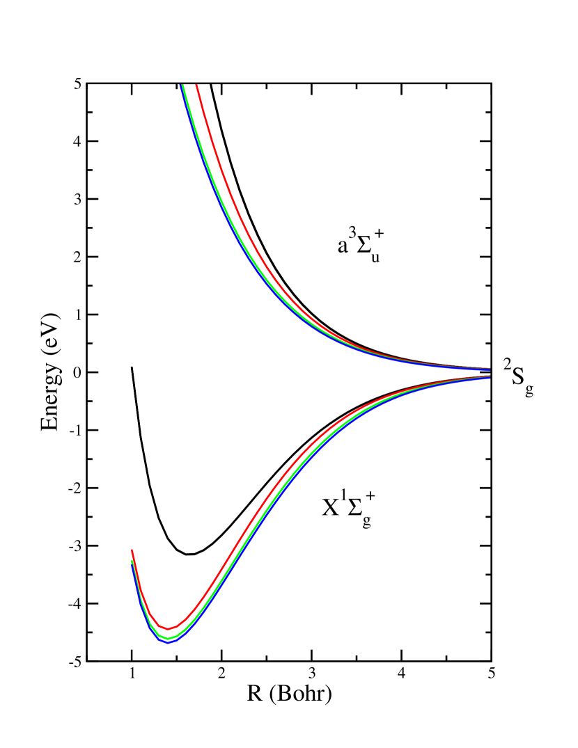
Figure 2: Diatomic-hydrogen interaction energies (lowest two states). Black, 1s-only solutions; Red, VB1-single-excit.; Green, VB2-single-excit.; Blue, VB3-single-excit. Asymptotic atomic state on the right.

Figure 3 shows some similar results for CH. The thicker lines (consistently less bound) are the VB3 no-excitation results. The thinner lines are for the VB3 basis with up to single excitation on each atom. It should be noted that these (and later reported polyatomic energies) are given in terms of a total, uncorrected atomization energy, an especially stringent test of theoretical methods, particular when used for homolytic bond cleavage.⁴⁴

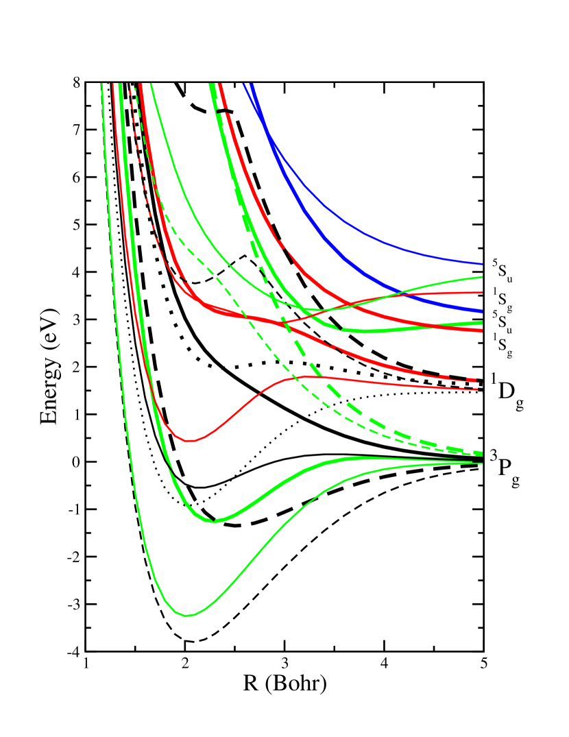
Figure 3: Diatomic CH interaction energies dissociating to the lowest four asymptotes in the VB3 basis. Thicker curves-no excitation; thinner curves-single excitation. Solid lines-$\Sigma$; dashed lines-$\Pi$, dotted lines-$\Delta$. Black-doublets (including ${}^{2}\Sigma^{-}$); green-quartets; blue-sextets; exception: red-${}^{2}\Sigma^{+}$. Asymptotic carbon asymptotes paired with $\mathrm{{}^{2}S_{g}}$ hydrogen are noted on the right; energy differences in the higher asymptotes can be noted in accord with the values in table 2.

The results calculated by more conventional orbital-based CI techniques in eq. 3 and those in the atomic state basis of eq. 12 are identical. Therefore comparison of the atomic state bases (tabs. 1 and 2) and the degree of diatomic binding supported by each, illustrate the perspective which the Spectral Theory provides on the importance of excited atomic states, even those above the ionization threshold, for molecular binding. This is true in the case of hydrogen where there is a one-to-one correspondence between orbitals and states as well as in carbon with its multi-electron character.

In moving from diatomic to polyatomic calculations, although all states are likely important to some degree, it might be supposed that aggregate binding may be mostly attributable to the most tightly bound diatomic states. Table 4 contains the energy minima for the low-lying diatomic curves for side-by-side comparison. (As in the previous table, the two additional columns in this and the following table will be discussed subsequently.) In lieu of experimental values the results of high-level calculations^{45, 46} are given for comparison.

It should be appreciated that although the underlying CI-based methods (eq.  3) are both size-consistent and variational, the variational discrepancies of a diatom at its equilibrium separation and at infinite separation may be different in magnitude. Thus the diatoms may be calculated to be over or underbound in a given finite basis.

Table 3: Diatomic binding energies (eV)

Basis	VB3*a	VB1	VB2	VB3	Cb	Db	Ref.
CH Multiplicityc	140	19,656	102,900	386,260	140	2856
Molec./State
$\mathrm{H_{2}\,^{1}\Sigma^{+}_{g}}$	3.2	4.4	4.6	4.7	4.7	4.7	4.7d
$\mathrm{CH\,^{2}\Pi}$	1.3	3.1	3.6	3.8	3.8	3.8	3.6e
$\mathrm{CH\,^{4}\Sigma^{-}}$	1.3	2.6	3.0	3.3	3.3	3.3	2.9e

^a Valence excitation only (see text) ^b Results included for comparison, not discussed until later section ^c See eq. 22 ^d Ref. 45 ^e Large basis MRCI, ref. 46

3.4 Polyatomic results

Figure 4 displays binding energies to total atomization calculated from the polyatomic matrix of eq. 20 for the four lowest states of the methylene molecule using the $\mathrm{H_{2}}$ and CH diatomic matrices calculated in the VB3 bases with limitation to valence-excitation. This system was an important touchstone in the demonstration of the qualitative and quantitative partnership of quantum chemistry with spectroscopy in the characterization of small molecules^{47, 48}. The optimization proceeds as follows. For a fixed HCH bond angle (ordinate) in the “V-shaped” $\mathrm{C_{2v}}$ molecule, the CH bond length is optimized and the binding energy (ordinate) is calculated. Thus, on the left, a ground-state diatomic hydrogen molecule is loosely associated with the indicated state of the carbon atom while on the right, the molecule takes on a symmetric collinear geometry and the states correlate with those of labeled electronic symmetry. The circles give high-level theoretical results (MRCI, ref. 49) for comparison. The evident underbinding in the Spectral Theory results is not surprising given the underbinding in the corresponding pair results in table 3 (first column) and is propagated to the polyatomic Hamiltonian matrix by the finite- and infinite-separation diatomic matrices. It is telling, however, that the subtle, qualitative angle-dependence is reproduced.

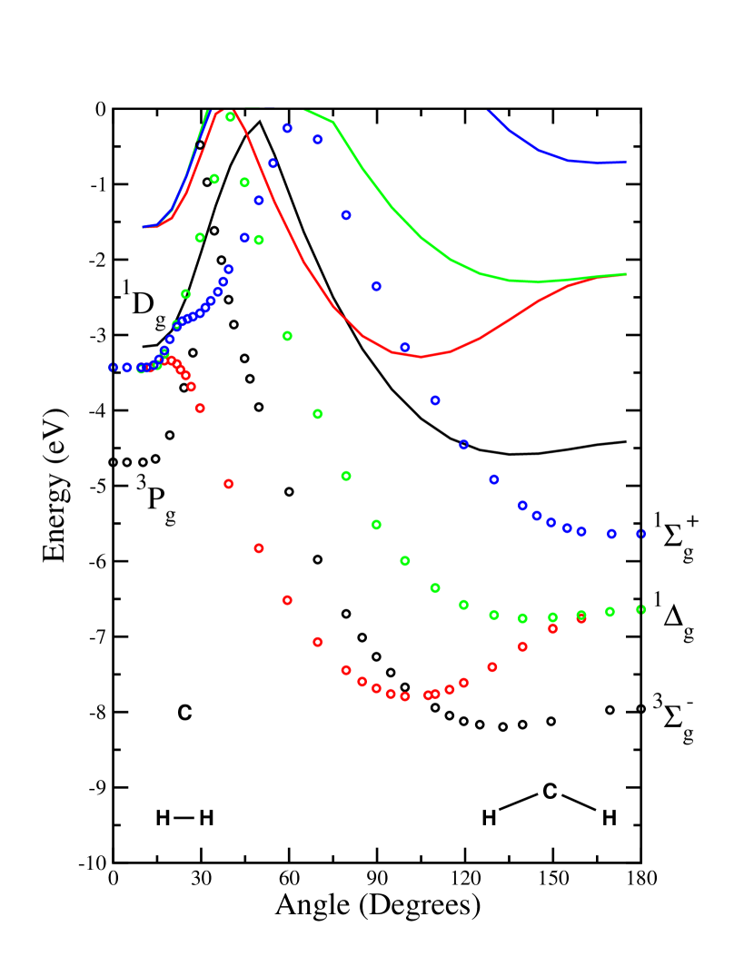
Figure 4: Optimized (see text for procedure and left and right asymptotic assignments) $\mathrm{CH_{2}}$ ($\mathrm{C_{2v}}$) total binding energies for fixed angles. Black-X$\mathrm{{}^{3}B_{1}}$; red-a$\mathrm{{}^{1}A_{1}}$; green-b$\mathrm{{}^{1}B_{1}}$; blue-c$\mathrm{{}^{1}A_{1}}$. Lines-Spectral Theory using the VB3 bases and only valence-excitation; circles-large-basis MRCI results, ref. 49.

For side-by-side comparison table 4 contains optimized (in all degrees of freedom) binding energies for a number of molecules containing a single carbon and a varying number of hydrogens using bases already discussed. Although the valence-excitation VB3 calculation is relatively primitive it is worth noting that the $\mathrm{CH_{5}}$ molecule (VB3* multiplicity 2,240) is unbound with respect to methane and hydrogen atom, at least initially alleviating concerns that a polyatomic theory build only from diatomic information may not observe chemical valence. (Because wave-function symmetry adaptation has not been implemented for all point groups $\mathrm{CH_{3}}$, $\mathrm{CH_{4}}$, and $\mathrm{CH_{5}}$ are calculated with $\mathrm{C_{2v}}$ electronic symmetry but with a higher symmetry nuclear geometry, as indicated in parentheses for each.)

Table 4: Polyatomic binding energies (eV)

Basis	VB3*a	VB1	Cb	Db	Ref.
$\mathrm{CH_{2}}$ Multiplicityc	280	235,872	280	34,272
Molec./State
$\mathrm{CH_{2}\,X:^{3}B_{1}}$	4.6	7.5	9.3	8.7	8.2d
$\mathrm{CH_{2}\,a:^{1}A_{1}}$	3.3	7.3	8.7	7.8	7.8d
$\mathrm{CH_{2}\,b:^{1}B_{1}}$	2.3		8.4	7.4	6.8d
$\mathrm{CH_{2}\,c:^{1}A_{1}}$	0.7		7.3	5.8	5.6d
$\mathrm{CH_{3}\,X(D_{3h})}$	6.5		14.9	13.4	12.6e
$\mathrm{CH_{4}\,X(T_{d})}$	10.4		19.6		17.1f
$\mathrm{CH_{5}\,X(D_{3h})}$	8.2		17.1

^a Valence excitation only ^b Results included for comparison, not discussed until later section ^c See eq. 22 ^d Ref. 49 ^e Ref. 50 ^f Ref. 51

4 Economization methods with results

The most direct method of increasing the fidelity of diatomic binding in the interacting pairs would be to increase the orbital and configuration bases going into the diatomic calculations of eq. 3, reducing the magnitude of the variational discrepancy for diatoms at finite and infinite separation and presumably reducing the difference between those discrepancies. The increase in the atomic state basis which would result would be disadvantageous because of the scaling in the size of the polyatomic problem (eq. 22). At least two alternate approximate approaches seem worth pursuing: sifting the configuration space for those expected to be most important to bonding and, at fixed atomic spectral size, directly injecting improved interaction energies into the pair matrices.

4.1 Reducing the size of the atomic spectrum

It is desirable to prune the atomic spectra (tabs.  1 and 2) by selecting or constructing only those states especially important for molecular binding. By way of example, consider the single-excitation, atomic-spectral basis for carbon labeled “VB3” in tab. 2) which has a multiplicity of 6230. The present focus is on describing low-lying polyatomic states and this search for a pruned atomic basis began with the presumption that low-lying atomic states are the most important. Initial efforts therefore eliminated altogether atomic states in the phase-consistent basis of eq. 5 with an energy above a fixed threshold (for example those above the $\mathrm{{}^{3}P_{g}(1)}$, $\mathrm{{}^{1}D_{g}(1)}$, $\mathrm{{}^{1}S_{g}(1)}$, and $\mathrm{{}^{5}S_{u}}$ states in carbon). This was surprisingly ineffective, presumably because of the total neglect of the above-threshold, valence-excited states.

The next attempt involved performing an initial atomic calculation in a large configuration set and examining the results of eq. 2. The Young tableaux supporting complete manifolds (right-hand side) were sifted based on their population-based contribution to a set of preselected lowest-energy atomic states (left-hand-side), for example the four lowest carbon state manifolds. Those with a contribution exceeding a threshold value were retaining for a second phase of atomic CI in a reduced configuration set. By adjusting the threshold, Young-tableau bases of varying size could be defined and carried forward into the construction of diatomic matrices. This was only partially successful as it seemed to still relatively devalue the valence-excited states which were not able to be isolated, but whose spectral density was spread among several of the higher energy states.

Finally a two-step procedure, completely within the atomic calculations, was employed to select the atomic-tableau functions. The orbitals of a large basis were divided into an inner set and an outer set. (In the frozen-core carbon example it was natural to put the 2s and 2p orbitals in the inner set.) A list of reference valence tableaux, indexed by r was then assembled from every allowable occupation of the inner orbitals. The vector-matrix form of eq. 2 is separated by components and every state, s on the left-hand-side was then assigned a “valence score,” $\mathrm{v_{s}}$, based upon the summed contributions of the reference configurations to it.

$$\mathrm{v_{s}}=\sum_{\mathrm{r}}\Phi_{\mathrm{r}}\mathrm{V_{rs}}$$ (23)

In a second step each of the tableau in the larger configuration set, indexed by k, was given a composite score, $\mathrm{t_{k}}$: the product of the contribution of the tableau to a state and the valence score of that state, summed over all the atomic states.

$$\mathrm{t_{k}}=\sum_{\mathrm{s}}\mathrm{v_{s}}\mathrm{V_{ks}}$$ (24)

This would quantify the relative importance of individual tableau, but as the Spectral Theory is founded upon using whole atomic manifolds (such as those listed, e.g in eqs. 17 and 18), a further manipulation is required. The tableaux can be partitioned into sets, indexed by q, which together support distinct manifolds. The collective importance of each set, $\mathrm{M_{q}}$ in number with each indexed by $\mathrm{k_{q}}$ can then be quantified by averaging the tableau weight over the set:

$$\mathrm{t_{q}}={1\over\mathrm{M_{q}}}\sum_{\mathrm{k_{q}}}\mathrm{t_{kq}}$$ (25)

Sets of tableaux with an averaged score above an adjustable threshold were then excluded or retained and this procedure provided configuration sets of varying size and fidelity to the original set. In this way, the variable valence-content of excited states could be flexibly accounted for, even while focusing on the lower, more energy-accessible states presumably most important for binding. For nonhydrogen atoms this procedure also allows a fine-tuning in the size of the atomic-state bases intermediate between the multiplicities (Tab. 2) which arise directly from the orbitals employed and the degree of excitation. Note that this basis reduction is propagated to the polyatomic dimension because of its polynomial scaling in the number of atomic states (eq. 22).

Table 2 shows term energies for two of these bases formed by selecting tableaux from all 6230 of those of the single-excitation VB3 calculation. That labeled “A” is obtained with a set threshold of 0.07, while the larger basis “B” uses 0.01. By way of example, basis “A” adds to the 70 states of eq. 17, 168 states of 22 new manifolds of term symmetries:

$$\mathrm{{}^{5}P_{g}},\mathrm{{}^{3}P_{g}},\mathrm{{}^{3}P_{u}},\mathrm{{}^{1}P_{u}},\mathrm{{}^{1}P_{g}},\mathrm{{}^{3}D_{g}},\mathrm{{}^{3}F_{u}},\mathrm{{}^{3}S_{g}},\mathrm{{}^{1}D_{g}},\mathrm{{}^{3}D_{g}},\mathrm{{}^{1}D_{u}},\\ \mathrm{{}^{3}P_{u}},\mathrm{{}^{3}D_{u}},\mathrm{{}^{1}F_{u}},\mathrm{{}^{3}S_{g}},\mathrm{{}^{1}P_{u}},\mathrm{{}^{3}P_{g}},\mathrm{{}^{3}P_{g}},\mathrm{{}^{1}S_{g}},\mathrm{{}^{1}P_{g}},\mathrm{{}^{1}D_{g}},\mathrm{{}^{1}S_{g}}$$ (26)

By making the threshold value sufficiently large, the valence-excited basis is recovered; setting it very low will give back the original, full single-excitation basis.

Figure 5 displays diatomic CH results for these reduced bases. For comparison the lines redisplay the single-excitation results of the VB3 basis from Fig. 3 (same color and line dash pattern so that symmetries can be assigned). In corresponding colors, and often difficult to distinguish, circles and squares show the results for the VB3 hydrogen basis paired with bases “A” and “B.” This procedure seems only partially successful in decreasing the size of the atomic spectrum while yielding sufficiently bound diatomic wells.

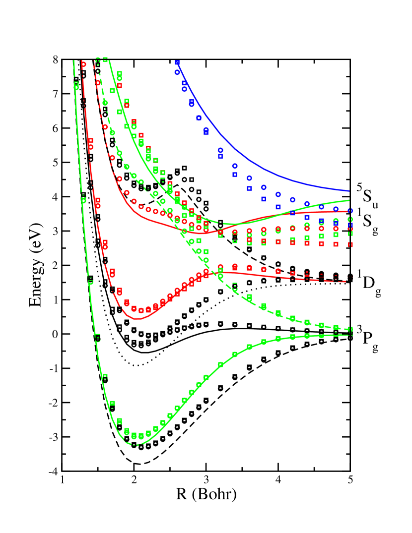
Figure 5: CH interaction energies with reduced carbon-atom spectral basis. Lines are identical to the thinner lines of Fig. 3, VB3, single excitation (same color and line dash pattern and labeled with asymptotic carbon state). Circles-basis “A”; squares-basis “B”; same color scheme as corresponding lines.

4.2 Injecting improved interaction energies

This means of improving the description of bonding in molecular aggregates for fixed atomic-spectral dimension can most easily be understood with reference to eq. 12. For a relatively small basis, the diatomic matrix ${\bf H}_{\bf d}^{(\alpha,\beta)}(R_{\alpha\beta})$ for each of the archived values of $R_{\alpha\beta}$ can be diagonalized, yielding ${\bf V}_{{\bf H}_{\bf d}}^{(\alpha,\beta)}(R_{\alpha\beta})$ and the interaction-energy eigenvalues along the diagonal of ${\bf E}^{(\alpha,\beta)}(R_{\alpha\beta})$. Selected, in this case low-energy, eigenvalues can then be replaced with values calculated using a larger configuration set (and shifted to reflect the difference in atomic ground-state energies). This combines a superior treatment of binding in the low-energy states with a reduced, but still complete (in the smaller basis), description of the excited states. The inverse of the original ${\bf V}_{{\bf H}_{\bf d}}^{(\alpha,\beta)}(R_{\alpha\beta})$ is right-multiplied on each side of eq. 12 yielding new “hybrid basis” diatomic matrices.

Figure 6 illustrates in more detail the components of these fused archive matrices. The black and green curves are all the diatomic curves which result from the smaller calculation with only valence excitation within the VB3 basis. The green curves are the (relatively underbound) curves already displayed in Fig. 3 as the thicker lines. The black curves are all the remaining diatomic states in this basis and have not been displayed heretofore. The significant break between the asymptotic energies of these two sets of curves should be noted and compared to the carbon-atom state energies of tab. 2.

The red curves are the diatomic results for states which dissociate to the four lowest carbon-atom asymptotes for single-excitation out of the valence reference space using the same basis. These were previously displayed in Fig. 3 as the thinner lines. Substituting the red curves in preference to their green counterparts gives increased binding in the lower diatomic states even if it may distort some of the higher interactions. (Note especially the avoided crossing prominent near R=2.5 Bohr.) In tables 3 and 4 the basis which results from this procedure is labeled “C.” Basis “D” is obtained from combining the same lower diatomic curves with the higher curves of the carbon basis labeled “A” in table 2 and described in the previous section.

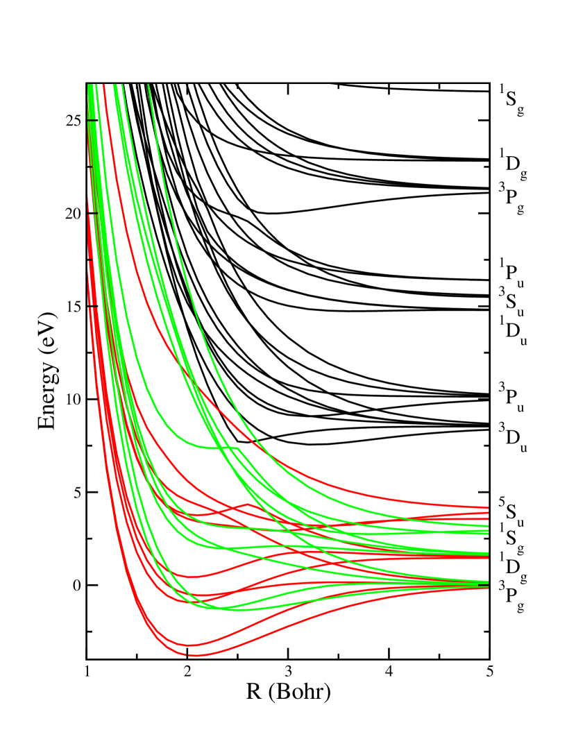
Figure 6: CH potential energy curves relevant for construction of the “A” fused-diatomic basis. For states dissociating to the lowest four asymptotes, the red curves (single-excitation VB3) are substituted for their valence-excitation analogues, the green curves to provide a basis with the same size as the no-excitation VB3, but increased binding in the low-energy states.

Figure 7 shows results for $\mathrm{CH_{2}}$, repeating the optimization procedure of Fig. 4 for bases “C” (solid lines) and “D” (dashed lines) (along with the same reference, high-level theoretical results). The injection of diatomic curves from higher-level calculations might seem somewhat artificial (especially if pursued too aggressively) but at least in this example does not seem to result in catastrophic distortion of the polyatomic results. These and the results in table 4 illustrate that fairly economical bases can furnish results in substantial agreement with more expensive theoretical methods.

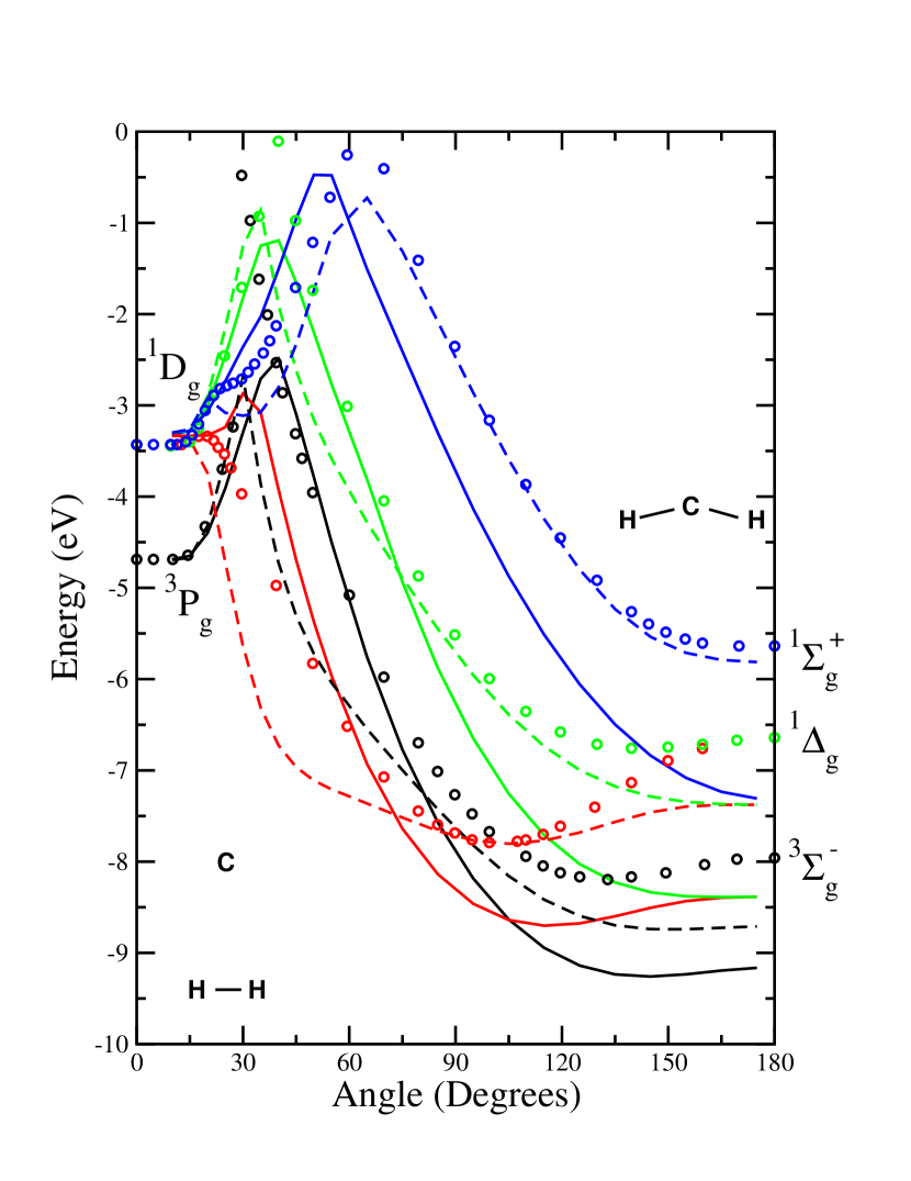
Figure 7: Optimized $\mathrm{CH_{2}}$($\mathrm{C_{2v}}$) binding energies for fixed angles (same optimization procedure, state colors and asymptotic channels as in Fig. 4). Solid lines-Spectral Theory using basis “C”; dashed lines-Spectral Theory using basis “D”; circles-large-basis MRCI results, ref. 49.

5 Continuing developments and conclusions

The finite-basis, pairwise-antisymmetrized form of the Spectral Theory of chemical bonding has been described and applied to the ground and low-excited states of some prototypical small hydrocarbons to illustrate its characteristics. Progress has also been reported on approximations to minimize the number of atomic states necessary to faithfully describe atomic and diatomic contributions. As the total polyatomic basis dimension is polynomial in atomic-state number but exponential in the number of atoms, application of this theory to larger molecules will require further attention to breaking the exponential scaling. In particular, future reports will describe economizing approximations inspired by density-matrix renormalization group theory^{52, 53, 54} and utilizing some unique simplifications which result in application of these methods to pairwise Hamiltonians (eq. 20).

6 Acknowledgments

I would like to acknowledge Peter W. Langhoff for valuable discussions concerning this work and related approaches, Jerry Boatz for his ready ear and helpful comments, Wayne Kalliomaa and Stefan Schneider for their supporting encouragement, and Mike Berman for significant early funding.

References

- Ball 2011 Ball, P. Beyond the bond. Nature 2011, 469, 26–28
- Bader 1990 Bader, R. Atoms in molecules: A quantum theory; Clarendon: Oxford, 1990
- Blanco et al. 2005 Blanco, M.; Pendás, A.; Francisco, E. Interacting quantum atoms: A correlated energy decomposition scheme based on the quantum theory of atoms in molecules. J. Chem. Theory Comput. 2005, 1, 1096–1109
- Francisco et al. 2006 Francisco, E.; Pendás, A.; Blanco, M. A molecular energy decomposition scheme for atoms in molecules. J. Chem. Theory Comput. 2006, 2, 90–102
- Rychlewski and Parr 1986 Rychlewski, J.; Parr, R. The atom in a molecule: A wave function approach. J. Chem. Phys. 1986, 84, 1696–1703
- Parr et al. 2005 Parr, R.; Ayers, P.; Nalewajski, R. What is an atom in a molecule? J. Phys. Chem. A 2005, 109, 3957–3959
- Ruedenberg and Schwarz 2013 Ruedenberg, K.; Schwarz, W. In Pioneers of quantum chemistry; Strom, E., Wilson, A., Eds.; Amer. Chem. Soc.: Washington DC, 2013; pp 1–45
- Ruedenberg 2022 Ruedenberg, K. Atoms and interatomic bonding synergism inherent in molecular electronic wave functions. J. Chem. Phys. 2022, 157, 024111
- Herbert 2019 Herbert, J. Fantasy versus reality in fragment-based quantum chemistry. J. Chem. Phys. 2019, 151, 170901–170938
- Langhoff 1996 Langhoff, P. Spectral theory of physical and chemical binding. J. Phys. Chem. 1996, 100, 2974–2984
- Langhoff et al. 2002 Langhoff, P.; Hinde, R.; Boatz, J.; Sheehy, J. Spectral theory of the chemical bond. Chem. Phys. Lett. 2002, 358, 231–236
- Langhoff et al. 2002 Langhoff, P.; Boatz, J.; Hinde, R.; Sheehy, J. In Low-lying potential energy surfaces; Hoffmann, M., Dyall, K., Eds.; Amer. Chem. Soc.: Washington DC, 2002
- Langhoff et al. 2004 Langhoff, P.; Boatz, J.; Hinde, R.; Sheehy, J. Atomic spectral methods for molecular electronic structure calculations. J. Chem. Phys. 2004, 121, 9323–9342
- Langhoff et al. 2004 Langhoff, P.; Boatz, J.; Hinde, R.; Sheehy, J. In Fundamental world of quantum chemistry; E.J. Brändas, E. K., Ed.; Kluwer: Amsterdam, 2004; Vol. III; pp 97–114
- Langhoff et al. 2008 Langhoff, P.; Hinde, R.; Mills, J.; Boatz, J. Spectral-product methods for electronic structure calculations. Theoret. Chem. Acc. 2008, 120, 199–213
- Ben-Nun et al. 2009 Ben-Nun, M.; Mills, J.; Hinde, R.; Winstead, C.; Boatz, J.; Gallup, G.; Langhoff, P. Atomic spectral-product representations of molecular electronic structure: metric matrices and atomic-product composition of molecular eigenfunctions. J. Phys. Chem. A 2009, 113, 7687–7697
- Mills et al. 2016 Mills, J.; Ben-Nun, M.; Rollin, K.; Bromley, M.; Li, J.; Hinde, R.; Winstead, C.; Sheehy, J.; Boatz, J.; Langhoff, P. Atomic spectral methods for ab initio molecular electronic energy surfaces: transition from small-molecule to biomolecular-suitable approaches. J. Phys. Chem. B 2016, 120, 8321–8337
- Langhoff et al. 2018 Langhoff, P.; Mills, J.; Boatz, J. Atomic-pair theorem for universal matrix representatives of molecules and atomic clusters in non-relativistic Born-Oppenheimer approximation. J. Math. Phys. 2018, 59, 072105
- Mills et al. 2018 Mills, J.; Boatz, J.; Langhoff, P. Quantum-mechanical definition of atoms and their mutual interactions in Born-Oppenheimer molecules. Phys. Rev. A 2018, 98, 012506
- Moffitt 1951 Moffitt, W. Atoms in molecules and crystals. Proc. Royal Soc. A. 1951, 210, 245–268
- Moffitt 1954 Moffitt, W. Atomic valence states and chemical binding. Reports Prog. Phys. 1954, 17, 173–200
- Ellison 1963 Ellison, F. A method of diatomics in molecules. I. General theory and application to . J. Amer. Chem. Soc. 1963, 85, 3540–3544
- Ellison et al. 1963 Ellison, F.; Huff, N.; Patel, J. A method of diatomics in molecules. II. and . J. Amer. Chem. Soc. 1963, 85, 3544–3547
- Ellison and Patel 1964 Ellison, F.; Patel, J. A method of diatomics in molecules. III. and (X = H, F, Cl, Br, and I). J. Amer. Chem. Soc. 1964, 86, 2115–2119
- Gallup 2002 Gallup, G. Valence bond methods: Theory and applications; Cambridge Univ. Press: Cambridge, 2002
- Chisholm 1976 Chisholm, C. Group Theoretical Techniques in Quantum Chemistry; Academic: London, 1976
- Wilson 2003 Wilson, S. In Handbook of Molecular Physics and Quantum Chemistry; Wilson, S., Ed.; Wiley: Chichester UK, 2003; Vol. 1; pp 369–379
- Edmonds 1974 Edmonds, A. Angular momentum in quantum mechanics, corrected and revised, second ed.; Princeton Univ.: Princeton, 1974
- Lomont 1959 Lomont, J. Applications of finite groups; Academic: New York, 1959
- Claverie 1971 Claverie, P. Theory of intermolecular forces. I. On the inadequacy of the usual Rayleigh-Schrödinger perturbation method for the treatment of intermolecular forces. Intern. J. Quantum Chem. 1971, 5, 273–296
- McWeeny 1989 McWeeny, R. Methods of molecular quantum mechanics, 2nd ed.; Academic: London, 1989; Chapter 4
- Löwdin 1970 Löwdin, P. On the nonorthogonality problem. Adv. Quantum Chem. 1970, 5, 185–199
- Srivastava 2000 Srivastava, V. A unified view of the orthogonalization methods. J. Phys. A: Math. Gen. 2000, 32, 6219–6222
- Hamermesh 1964 Hamermesh, M. Group theory and its application to physical problems, corrected second ed.; Addison-Wesley: Reading Mass., 1964
- Ema et al. 2003 Ema, I.; de la Vega, J.; Ramírez, G.; López, R.; Rico, J.; Meissner, H.; Paldus, J. Polarized basis sets of slater-type orbitals: H to Ne atoms. J. Comput. Chem. 2003, 24, 859–868
- Rico et al. 2001 Rico, J.; López, R.; Aguado, A.; Ema, I.; Ramírez, G. New program for molecular calculations with Slater-type orbitals. Intern. J. Quantum Chem. 2001, 81, 148–153
- 37 \urlhttp://sourceforge.net/projects/molcrunch, accessed, 5 Jan. 2023
- Gallup 1982 Gallup, G. Iterative calculation of eigenvalues and eigenvectors of large, real matrix systems with overlap. J. Comput. Chem. 1982, 3, 127–129
- Stathopoulos and McCombs 2010 Stathopoulos, A.; McCombs, J. PRIMME: PReconditioned Iterative MultiMethod Eigensolver: Methods and software descriptions. ACM Transact. Math. Software 2010, 37, 1–30
- 40 \urlhttp://www.cs.wm.edu/ andreas/software, accessed, 5 Jan. 2023
- Press et al. 2007 Press, W.; Teukolsky, S.; Vetterling, W.; Flannery, B. Numerical recipes: The art of scientific computing; Cambridge Univ. Press: Cambridge, 2007
- 42 \urlhttp://www.mcs.anl.gov/petsc, accessed, 5 Jan. 2023
- 43 \urlhttp://www.nist.gov/pml/atomic-spectra-database, accessed, 5 Jan. 2023
- Dutta and Sherrill 2003 Dutta, A.; Sherrill, C. Full configuration interaction potential energy curves for breaking bonds to hydrogen: An assessment of single-reference correlation methods. J. Chem. Phys. 2003, 118, 1610–1619
- Kolos and Wolniewicz 1968 Kolos, W.; Wolniewicz, L. Improved theoretical ground-state energy of the hydrogen molecule. J. Chem. Phys. 1968, 49, 404–410
- Kalemos et al. 1999 Kalemos, A.; Mavridis, A.; Metropoulos, A. An accurate description of the ground and excited states of CH. J. Chem. Phys. 1999, 111, 9536–9548
- Goddard III 1985 Goddard III, W. Theoretical chemistry comes alive: Full partner with experiment. Science 1985, 227, 917–923
- Schaefer 1986 Schaefer, H. Methylene: A paradigm for computational quantum chemistry. Science 1986, 231, 1100–1107
- Kalemos et al. 2004 Kalemos, A.; Jr., T. D.; Mavridis, A.; Harrison, J. revisited. Canadian J. Chem. 2004, 82, 684–693
- A. Zanchet 2016 A. Zanchet, M. S. A. G.-V., L. Bañares An ab initio study of the ground and excited electronic states of the methyl radical. Phys. Chem. Chem. Phys. 2016, 18, 33195–33203
- van Harrevelt 2006 van Harrevelt, R. Photodissociation of methane: Exploring potential energy surfaces. J. Chem. Phys. 2006, 125, 124302
- White and Noack 1992 White, S.; Noack, R. Real-space quantum renormalization groups. Phys. Rev. Lett. 1992, 68, 3487–3490
- White 1992 White, S. Density matrix formulation for quantum renormalization groups. Phys. Rev. Lett. 1992, 69, 2863–2866
- White 1993 White, S. Density-matrix algorithms for quantum renormalization groups. Phys. Rev. B 1993, 48, 10345–10356