Equivariance with Learned Canonicalization Functions

Abstract

Symmetry-based neural networks often constrain the architecture in order to achieve invariance or equivariance to a group of transformations. In this paper, we propose an alternative that avoids this architectural constraint by learning to produce canonical representations of the data. These canonicalization functions can readily be plugged into non-equivariant backbone architectures. We offer explicit ways to implement them for some groups of interest. We show that this approach enjoys universality while providing interpretable insights. Our main hypothesis, supported by our empirical results, is that learning a small neural network to perform canonicalization is better than using predefined heuristics. Our experiments show that learning the canonicalization function is competitive with existing techniques for learning equivariant functions across many tasks, including image classification, $N$-body dynamics prediction, point cloud classification and part segmentation, while being faster across the board.

1 Introduction

The problem of designing machine learning models that properly exploit the structure and symmetry of the data is becoming more important as the field is broadening its scope to more complex problems. In multiple applications, the transformations with respect to which we require a model to be invariant or equivariant are known and provide a strong inductive bias (e.g.,  Bronstein et al., 2021; Bogatskiy et al., 2022; van der Pol et al., 2020; Mondal et al., 2020; Celledoni et al., 2021).

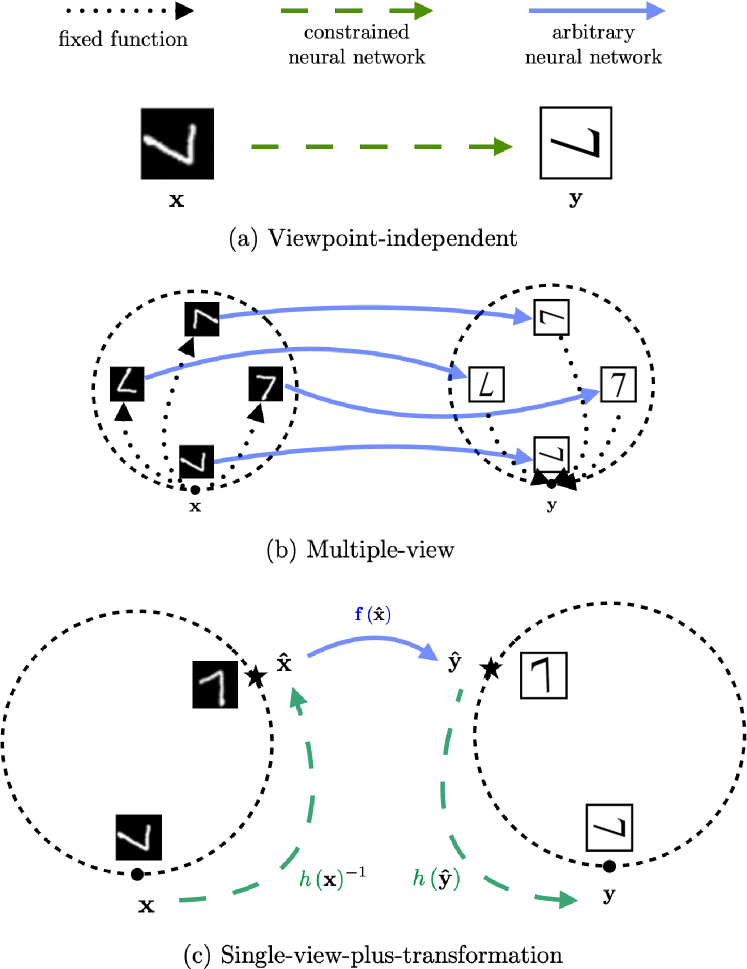
Figure 1: A classification of different frameworks for equivariant predictions. In this example, the task is to restyle an MNIST digit in a rotation equivariant way. We propose a class of models that falls in the single-view-plus-transformation framework.

As is often the case, taking a step back and drawing analogies with human cognition is fruitful here. Human pattern recognition handles some symmetries with relative ease. When data is transformed in a way that preserves its essential characteristics, we precisely know if and how we should adapt our response.

One context in which this has been particularly well-studied in cognitive science is visual shape recognition. Experiments have shown that subjects can accurately distinguish between different orientations of an object and actual modifications to the structure of an object (Shepard & Metzler, 1971; Carpenter & Eisenberg, 1978).

There are multiple ways in which this could be achieved. According to Tarr & Pinker (1989), theories of invariant shape recognition broadly fall into three categories: viewpoint-independent models, in which object representations depend only on invariants features, multiple-view models in which an object is represented as a set of representations corresponding to different orientations, and single-view-plus-transformation models in which an object is converted to a canonical orientation by a transformation process.

Correspondingly, similar ideas have been explored in deep learning to achieve equivariance; see Figure 1. Models that impose equivariance through constraints in the architecture (Shawe-Taylor, 1989; Cohen & Welling, 2016a; Ravanbakhsh et al., 2017) or that only use invariants as inputs (Villar et al., 2021) can be seen as belonging to the viewpoint-independent type since the dependence of the model on symmetry transformations is trivial. The multiple-view approach includes models that symmetrize the input by averaging over all the transformations or a subset of them (Manay et al., 2006; Benton et al., 2020; Yarotsky, 2022; Puny et al., 2022). By contrast, the transformation approach has seen less interest. This is all the more surprising considering that evidence from cognitive science suggests that this approach is used in human visual cognition (Shepard & Metzler, 1971; Carpenter & Eisenberg, 1978; Hinton & Parsons, 1981). When presented with a rotated version of an original pattern, the time taken by humans to do the association is proportional to the rotation angle, which is more consistent with the hypothesis that we perform a mental rotation.

Present work

We introduce a systematic and general method for equivariant machine learning based on learning mappings to canonical samples. We hypothesize that among all valid canonicalization functions, some will lead to better downstream performance than others. Rather than trying to hand-engineer these functions, we may let them be learned in an end-to-end fashion with a prediction neural network. Our method can readily be used as an independent module that can be plugged into existing architectures to make them equivariant to a wide range of groups, discrete or continuous. Our approach enjoys similar expressivity advantages to methods like frame averaging by Puny et al. (2022), but has several added benefits. It is simpler, more efficient, and replaces hand-engineered frames for each group by a systematic end-to-end learning approach.

Our contributions are as follows:

Novel Framework

We introduce a general framework for equivariance to a variety of groups based on mappings to canonical samples. This framework can be plugged into any existing non-equivariant architecture.

Theoretical Guarantees

We prove that in some settings, such models are universal approximators of equivariant functions.

Practical Performance

We perform experiments that show that the proposed method achieves excellent results on images, physical dynamical systems and point clouds. We also support our hypothesis that learning the canonicalization function is a better strategy than designing it by hand.

Efficient Implementations

We provide multiple variants of efficient implementations of this framework to specific domains.

2 Related Works

Methods based on heuristics to standardize inputs have been around for a long time (Yüceer & Oflazer, 1993; Lowe, 2004). However, these approaches require significant hand-engineering and are difficult to generalize. An important early work is the Spatial Transformer Network (Jaderberg et al., 2015) which learns input transformations to facilitate processing in a downstream vision task. PointNet (Qi et al., 2017a) also proposed to learn an alignment network to encourage invariance for point cloud analysis. However, these approaches are closer to regularizers and provide no equivariance guarantees. The works of (Esteves et al., 2018b; Tai et al., 2019) provided equivariant versions of the Spatial Transformer using an approach based on canonical coordinates. One limitation of this approach is that it does not exactly handle equivariance to groups that are larger in dimension than the dimension of the data grid. Some recent works have proposed using learned coordinate frames for point clouds (Kofinas et al., 2021; Luo et al., 2022; Du et al., 2022). We provide theoretical and experimental evidence that the neural networks for canonicalization can be made much shallower and simpler without affecting performance. Bloem-Reddy & Teh (2020), introduce the concept of representative equivariant, which is similar to what we implement in this work. Finally, other recent works (Winter et al., 2022; Vadgama et al., 2022) have proposed to use canonicalization in an autoencoding setup.

3 Canonicalization Functions

3.1 Problem Setting

We are interested in learning functions $\mbox{\boldmath$\phi$}:\mathcal{X}\to\mathcal{Y}$ with inputs $\mathbf{x}\in\mathcal{X}$ and outputs $\mathbf{y}\in\mathcal{Y}$ belonging to finite-dimensional normed vector spaces. We will consider a set of linear symmetry transformations $T\subset\mathrm{GL}\left(\mathcal{X}\right)$, where $\mathrm{GL}\left(\mathcal{X}\right)$ is the set of invertible matrices over the vector space $\mathcal{X}$. This is described by a group representation $\rho:G\to T$, where $G$ is an abstract group. Without loss of generality, we can assume that $\rho$ is a group isomorphism. Therefore, the inverse $\rho^{-1}:T\to G$ is defined. In this context, a function $\phi$ is $G$-equivariant if

$$\mbox{\boldmath$\phi$}\left(\rho\left(g\right)\mathbf{x}\right)=\rho^{\prime}\left(g\right)\mbox{\boldmath$\phi$}\left(\mathbf{x}\right),\ \forall\ g,\mathbf{x}\in G\times\mathcal{X},$$ (1)

where the group action $\rho$ on the input and the group action $\rho^{\prime}$ on the output will be clear from the context. In particular, when $\rho^{\prime}\left(g\right)=I$, we say that $\phi$ is invariant. We use $\rho\left(H\right)$ to denote the image of the subset $H$ under $\rho$.

The set $\rho\left(G\right)\mathbf{x}=\left\{\rho\left(g\right)\mathbf{x}\mid\forall\ g\in G\right\}$ is the orbit of the element $\mathbf{x}$. It is the set of elements to which $\mathbf{x}$ can be mapped by the group action. The set of orbits denoted by $\mathcal{X}/G$ forms a partition of the set $\mathcal{X}$.

3.2 General Formulation

The invariance requirement on a function $\phi$ amounts to having all the members of a group orbit mapped to the same image by $\phi$. It is thus possible to achieve invariance by appropriately mapping all elements to a canonical orbit representative before applying any function. For equivariance, elements can be mapped to a canonical sample and, after a function is applied, transformed back according to their original position in the orbit. This can be formalized by writing the equivariant function $\phi$ in canonicalized form as

$$\mbox{\boldmath$\phi$}\left(\mathbf{x}\right)=h^{\prime}\left(\mathbf{x}\right)\mathbf{f}\left(h\left(\mathbf{x}\right)^{-1}\mathbf{x}\right),$$ (2)

where the function $\mathbf{f}:\mathcal{X}\to\mathcal{Y}$ is called the prediction function and the function $h:\mathcal{X}\to\rho\left(G\right)$ is called the canonicalization function. Here $h\left(\mathbf{x}\right)^{-1}$ is the inverse of the representation matrix and $h^{\prime}\left(\mathbf{x}\right)=\rho^{\prime}\left(\rho^{-1}\left(h\left(\mathbf{x}\right)\right)\right)$ is the counterpart of $h\left(\mathbf{x}\right)$ on the output.

Equivariance in Equation 2 is obtained for any prediction function if the canonicalization function is itself $G$-equivariant, $h\left(\rho\left(g\right)\mathbf{x}\right)=\rho\left(g\right)h\left(\mathbf{x}\right)\ \forall\ g,x\in G\times\mathcal{X}$.

It may seem like the problem of obtaining an equivariant function has merely been transferred in this formulation. This is, however, not the case: in Equation 2, the equivariance and prediction components are effectively decoupled. The canonicalization function $h$ can therefore be chosen as a simple and inexpressive equivariant function, while the heavy-lifting is done by the prediction function $\mathbf{f}$.

3.3 Partial Canonicalization and Lattice of Subgroups

A more general condition can be formulated, such that the decoupling is partial. This enables us to impose part of the symmetry constraint on the prediction network and use canonicalization for “additional” symmetries. This could, for example, be used to imbue a translation equivariant architecture, like a CNN, with rotation equivariance.

Theorem 3.1.

For some subgroup $K\leq G$, if $\forall\ g,\mathbf{x}\in G\times\mathcal{X}$ there exists a $k\in K$ such that

$$h\left(\rho\left(g\right)\mathbf{x}\right)=\rho\left(g\right)h\left(\mathbf{x}\right)\rho\left(k\right),$$ (3)

and the prediction function $\mathbf{f}$ is $K$-equivariant, then $\phi$ defined in Equation 2 is $G$-equivariant.

The proof follows in Appendix C. This is equivalent to saying that the canonicalization function should output a coset in $G/K$ in an equivariant way, the applied transformation being chosen arbitrarily within the coset.

This can be simplified when the group factors into a semi-direct product using the following result.

Theorem 3.2.

If $K$ is a normal subgroup such that $G\simeq J\ltimes K$, condition Equation 3 can be realized with a canonicalization function with image $\rho\left(J\right)$, and that is $J$-equivariant and $K$-invariant.

The proof follows in Appendix D. Going back to the example of using rotation canonicalization with a CNN, Theorem 3.1 says that the canonicalization function should output an element of the Euclidean group transforming equivariantly under rotations of the input. Since the translation subgroup is normal, Theorem 3.2 can be used to guarantee that the canonicalization network can always simply output a rotation.

In general, when $K=\left\{e\right\}$, only the canonicalization function is constrained, which is the case described at the beginning of the section. In the image domain, this would correspond to canonicalizing with respect to the full Euclidean group and using an MLP as a prediction function. The other extreme, given by $K=G$, corresponds to transforming the input in an arbitrary way and constraining the prediction function as is usually done in equivariant architectures like Group Equivariant Convolutional Neural Networks (G-CNNs) (Cohen & Welling, 2016b). These are, respectively, the single-view-plus-transformation and the viewpoint-independent implementations described in the introduction. Subgroups $\left\{e\right\}<K<G$ offer intermediary options; the lattice of subgroups of $G$, therefore, defines a family of models. Since equivariance to a smaller group is less constraining for the prediction function, set inclusion in the subgroup lattice is equivalent to increased expressivity for the corresponding models.

3.4 Universality Result

We can now introduce a more formal result on the expressivity of equivariant functions obtained with canonicalization functions. A parameterized function $\phi$ is a universal approximator of $G$-equivariant functions if for any $G$-equivariant continuous function $\psi$, any compact set $\mathcal{K}\subseteq\mathcal{X}$ and any $\epsilon>0$, there exists a choice of parameters such that $\norm{\mbox{\boldmath$\psi$}\left(\mathbf{x}\right)-\mbox{\boldmath$\phi$}\left(\mathbf{x}\right)}<\epsilon\ \forall\ \mathbf{x}\in\mathcal{K}$.

Theorem 3.3.

Let $\phi$ be a $G$-equivariant parameterized function given by Equation 2 and satisfying Equation 3 with $K\leq G$. Suppose that the canonicalization functions $h$ and $h^{\prime}$ are continuous. Then $\phi$ is a universal approximator of $G$-equivariant functions if the prediction function $\mathbf{f}$ is a universal approximator of $K$-equivariant functions.

The proof follows in Appendix E. The following corollary is especially relevant.

Corollary 3.4.

A $G$-equivariant parameterized function $\phi$ written as Equation 2 with a $G$-equivariant continuous canonicalization function and a multilayer perceptron (MLP) as a prediction function is a universal approximator of $G$-equivariant functions.

This result can significantly simplify the design of universal approximators of equivariant functions since a non-universal equivariant architecture for the canonicalization function can be combined with an MLP. In particular, notice that the universality of this scheme does not hinge on the expressivity of the canonicalization network.

We note that the framework encompasses a large space of design choices, with partial canonicalization to an arbitrary subgroup $K$. It may be useful in some cases to opt for partial canonicalization and defer some equivariance to the prediction function. This reduces the number of independent parameters of the prediction function, which can help with generalization and efficiency. A useful design pattern would therefore be to find the maximal subgroup $K$ of $G$, such that a universal approximator of $K$-equivariant functions can be efficiently implemented for the prediction function. Following Theorem 3.3, this allows universal approximation of $G$-equivariant functions.

4 Design of Canonicalization Functions

The canonicalization function can be chosen as any existing equivariant neural network architecture with the output being a group element; we call this the direct approach (figure 2(a)). For permutation groups and Lie groups, an equivariant multilayer perceptron (Shawe-Taylor, 1989; Finzi et al., 2021) can be used. We provide examples of implementations in the next section.

We also introduce an alternative method, which we call the optimization approach (Figure 2(b)). The canonicalization function can be defined as

$$h\left(\mathbf{x}\right)\in\operatornamewithlimits{arg\,min}_{\rho\left(g\right)\in\rho\left(G\right)}s\left(\rho\left(g\right),\mathbf{x}\right),$$ (4)

where $s:\rho\left(G\right)\times\mathcal{X}\to\mathbb{R}$ can be a neural network. When a set of elements minimize $s$, one is chosen arbitrarily. $s$ has to satisfy the following equivariance condition

$$s\left(\rho\left(g\right),\rho\left(g_{1}\right)\mathbf{x}\right)$$ (5)

$$=s\left(\rho\left(g_{1}\right)^{-1}\rho\left(g\right),\mathbf{x}\right),\ \forall g_{1}\in G,$$

and has to be such that argmin is a subset of a coset of the stabilizer of $\mathbf{x}$. This last condition essentially means that the minimum in each orbit should be unique up to input symmetry. In Appendix B, we prove that these are sufficient conditions to have a suitable canonicalization function.

The equivariance condition on $s$ can be satisfied using an equivariant architecture. Remarkably, it can also be satisfied using a non-equivariant function $E:\mathcal{X}\to\mathbb{R}$ and defining

$$s\left(\rho\left(g\right),\mathbf{x}\right)=E\left(\rho\left(g\right)^{-1}\mathbf{x}\right).$$ (6)

We will call the function $E$ energy. Intuitively, $E$ represents a distance between the input and the canonical sample of the orbit and is therefore minimized when $\rho\left(g\right)$ is the transformation that maps to the canonical sample.

This implementation presents a close analogy with the mental rotation phenomenon described in the introduction, as humans try to minimize the distance between their representation of an object and the canonical one. As such, it is expected that the optimization process will take more iterations when the input sample is farther away in orbit from the canonical sample. This is consistent with the experimental evidence for mental rotation (Shepard & Metzler, 1971; Carpenter & Eisenberg, 1978).

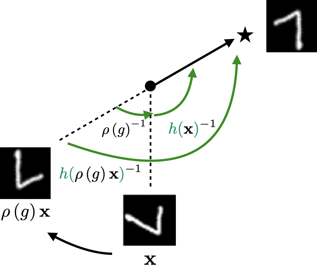
(a) Direct approach

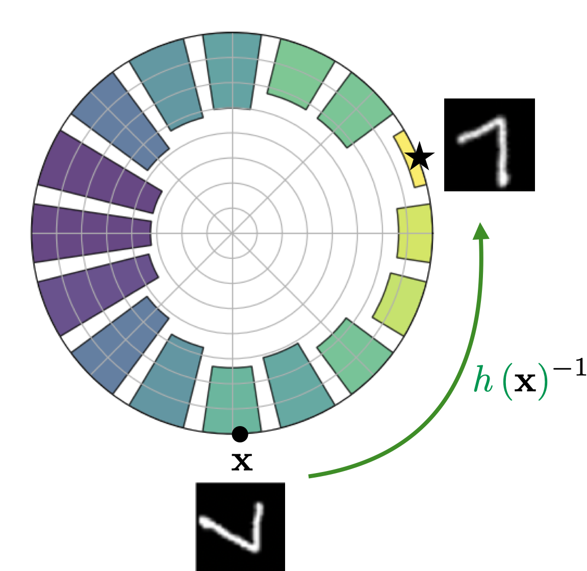
(b) Optimization approach

Figure 2: Two general approaches to canonicalization. In the direct approach, an equivariant neural network outputs the transformation. In the optimization approach, a function of the input is minimized to obtain the canonical sample.

Simultaneous minimization and learning of $s$ results in a bi-level optimization problem (Gould et al., 2016; Liu et al., 2021). This can be performed in a variety of ways, including using implicit methods (Blondel et al., 2022). Next, we elaborate on how suitable canonicalization functions can be obtained in different settings.

4.1 Euclidean Group

The Euclidean group $E\left(d\right)$ describes rotation, translation, and reflection symmetry. Domains in which this type of symmetry is especially relevant include computer vision, point cloud modelling and physics applications. Below we give design principles to obtain equivariant models for image and point cloud inputs.

Image Input.

Elements of the Euclidean group can be written as $\left(\mathbf{O},\mathbf{t}\right)$, where $\mathbf{O}\in\mathbb{R}^{n\times n}$ is an orthogonal matrix and $\mathbf{t}\in\mathbb{R}^{n}$ is an arbitrary translation vector. We consider the space of image inputs $I\in\mathcal{X}$ as given by a $2$ dimensional signal $I:\mathbb{R}^{2}\to\mathbb{R}^{C}$, where $C$ is the number of input channels. We adopt a continuous description to facilitate exposition, but in practice, all the operations are discretized using interpolation (Riba et al., 2020). This thus reduces to the $pnm$ group, which is the group of $n$-fold discrete rotations, reflections and discrete translations. The action of the representation on image inputs is defined by the following linear operator

$$[\rho\left(\mathbf{O},\mathbf{t}\right)\cdot I](\mathbf{p})=I(\mathbf{O}^{-1}(\mathbf{p}-\mathbf{t})),\quad\forall\mathbf{p}\in\mathbb{R}^{2},$$

where $\mathbf{p}$ is pixel position. The canonicalization function should output an element of the $E\left(2\right)$. It should also be $E\left(2\right)$-equivariant, such that $h\left(\rho\left(\mathbf{O},\mathbf{t}\right)\cdot{I}\right)={\rho\left(\mathbf{O},\mathbf{t}\right)}\cdot h\left(I\right)$.

This condition can be satisfied by using a Group Equivariant CNN (G-CNN) (Cohen & Welling, 2016a) and the optimization approach described above. To do this, we define the function to be optimized as $s:O\left(2\right)\times\mathbb{R}^{2}\times\mathcal{X}\to\mathbb{R}$. This can be reinterpreted as $s:\mathcal{X}\to\mathbb{R}^{O\left(2\right)\times\mathbb{R}^{2}}$, which means where the first dimension, a.k.a. the fiber, encodes rotation angles and $\mathbb{R}^{2}$ is associated with pixel positions. If $s$ is a G-CNN, it correctly satisfies the condition Equation 5, as image rotations act on the fiber and Euclidean transformations on the pixel positions. The canonicalization is then obtained by taking the $\operatornamewithlimits{arg\,min}$ over pixel positions and fibers

$$h\left(\mathbf{x}\right)\in\operatornamewithlimits{arg\,min}_{\left(\mathbf{O},\mathbf{t}\right)\in E(2)}s\left(\mathbf{x}\right)_{\left(\mathbf{O},\mathbf{t}\right)}.$$ (7)

This approach can be further simplified if we use a translation equivariant prediction network, such as a CNN-based architecture. As the translation group $T(2)$ is a normal subgroup of the Euclidean group $E(2)$, using Theorem 3.2, we only require the canonicalization function to be equivariant to $O(2)$. This means we can average over the spatial dimension in the output feature map of the canonicalization function and only need to take an $\operatornamewithlimits{arg\,min}$ along the rotation fiber dimension to identify the orientation of the image.

There are two potential problems with this approach. First, extending G-CNNs to a higher number of finer discrete rotations is computationally expensive, and it leads to artifacts. Second, we cannot backpropagate through the canonicalization function as the $\arg\min$ operation is not differentiable.

We can avoid the first problem by using a shallower network with a larger filter size. We empirically show why this is a sound choice for canonicalization function in Section 5. We use the straight-through gradient estimator (Bengio et al., 2013) to solve the second problem. Appendix I contains a PyTorch code snippet to perform the canonicalization function of images in a differentiable way using a G-CNN.

Point Cloud Input.

The $n+1$ dimensional representation of the Euclidean group (defined by concatenating a constant 1 to the original vectors) is defined in the following way

$$\rho{\left(\mathbf{O},\mathbf{t}\right)}=\begin{pmatrix}\mathbf{O}&\mathbf{t}\\ \mathbf{t}^{T}&1\end{pmatrix}.$$ (8)

We seek to define an $E\left(d\right)$-equivariant canonicalization function for point clouds. This can be done by defining it as $h\left(\mathbf{x}\right)=\rho{\left(h^{O}\left(\mathbf{x}\right),h^{t}\left(\mathbf{x}\right)\right)}$, where the function $h^{O}:\mathcal{X}\to\mathbb{R}^{n\times n}$ outputs the rotation and reflection and $h^{t}:\mathcal{X}\to\mathbb{R}^{n}$ the translation. Since the product of elements of $E\left(n\right)$ is given by $\left(\mathbf{O}_{1},\mathbf{t}_{1}\right)\left(\mathbf{O}_{2},\mathbf{t}_{2}\right)=\left(\mathbf{O}_{1}\mathbf{O}_{2},\mathbf{O}_{2}\mathbf{t}_{1}+\mathbf{t}_{2}\right)$, the equivariance condition requires that we have

$${h^{O}\left(\rho{\left(\mathbf{O},\mathbf{t}\right)}\mathbf{x}\right)}=\mathbf{O}h^{O}\left(\mathbf{x}\right),$$ (9)

$$h^{t}\left(\rho{\left(\mathbf{O},\mathbf{t}\right)}\mathbf{x}\right)={\mathbf{O}h^{t}\left(\mathbf{x}\right)+\mathbf{t}}.$$ (10)

This means that $h^{O}$ must be $O\left(d\right)$-equivariant and translation invariant, and that $h^{t}$ must be $E\left(d\right)$-equivariant. These constraints can be satisfied by using already existing equivariant architectures. Since most of the work will be done by a prediction function that can be very expressive, like Pointnet (Qi et al., 2017a), a simple and efficient architecture can be used for the canonicalization function, for example, Vector Neurons (Deng et al., 2021). The output of $h^{O}$ can be made an orthogonal matrix by having it output $n$ vectors and orthonormalizing them with the Gram-Schmidt procedure, which is itself equivariant (Appendix F).

Using Deep Sets (Zaheer et al., 2017a) as a backbone architecture would result in a universal approximator of $E\left(d\right)$ and permutation equivariant functions, following Theorem 3.3 and Theorem 1 of (Segol & Lipman, 2020).

4.2 Symmetric Group

The symmetric group $S_{n}$ over a finite set of $n$ elements contains all the permutations of that set. This group captures the inductive bias that input order should not matter. Domains for which $S_{n}$-equivariance is desirable include object modelling and detection, graph representation learning, and applications in language modelling.

$S_{n}$-equivariant canonicalization functions can be obtained with a direct approach using existing optimal transport solvers (Villani, 2009). For example, the Sinkhorn algorithm (Sinkhorn, 1964; Mena et al., 2018) solves the entropy-regularized optimal transport problem (Cuturi, 2013), which results in convex combinations of permutations (doubly-stochastic matrices) that are equivariant. In practice, this is an example of the implementation of canonicalization with the direct approach. Obtaining a permutation can also be framed as an optimization problem, which makes our optimization approach in Equation 4 relevant; problems like sorting (Blondel et al., 2020) and optimal transport (Blondel et al., 2018) are often formulated like this, which shows that this is a powerful paradigm.

5 Experiments

5.1 Image classification

We first perform an empirical analysis of the proposed framework in the image domain. We selected the Rotated MNIST dataset (Larochelle et al., 2007), often used as a benchmark for equivariant architectures. The task is to classify randomly rotated digits. In Table 1, we compare our method with different CNN and G-CNN (Cohen & Welling, 2016a) baselines. We denote the networks equivariant to $pn$ by putting it with the network’s name (e.g. G-CNN(p4)). The training and architecture details are provided in Section G.1. For the canonicalization function, we choose a shallow G-CNN with three layers. The first layer is a lifting layer which maps the signal in the pixel space to the group with filters that are the same size as the input image. This is followed by ReLU nonlinearity and group equivariant layers with $1\times 1$ filters.

Table 1: Comparison with the existing work for Rotated-MNIST.

Method Error % $\downarrow$ CNN (base) 4.90 $\pm$ 0.20 G-CNN (p4) 2.28 $\pm$ 0.00 G-CNN (p4 & = params) 2.36 $\pm$ 0.15 G-CNN (p64 & = params) 2.28 $\pm$ 0.10 Ours CN(PCA)-CNN 3.35 $\pm$ 0.21 CN(p4 & frozen)-CNN 3.91 $\pm$ 0.12 CN(OPT)-CNN 3.35 $\pm$ 0.00 CN(p4)-CNN 2.41 $\pm$ 0.10 CN(p64)-CNN 1.99 $\pm$ 0.10

We learn the canonicalization function end-to-end with a CNN as the prediction function (CN($pn$)-CNN). We also implement Equation 6 as CN(OPT)-CNN. Our $E$ converts the input image into a point cloud representation, which is fed into a PointNet that produces the energy. We use gradient descent to optimize this energy with respect to the input rotation for a small number of steps. This procedure is visualized in Figure 2(b).

For the pure G-CNN-based baseline, we provide the value reported by Cohen & Welling (2016a) and design a variant which has similar architecture to CNN (base) while matching the number of parameters of our CN(p4)-CNN. We call this G-CNN (p4 & = params).

Lastly, we consider variants where the canonicalization function is not learned. The first one is a G-CNN similar to CN($pn$) but with weights frozen at initialization. We call them CN(p4 & frozen)-CNN and CN(p64 & frozen)-CNN. For the second one, canonicalization is performed by finding the orientation of the digits using Principal Component Analysis (PCA) and we refer to it as CN(PCA)-CNN.

Results

As reported in Table 1 the direct canonicalization approach outperforms the CNN-based baseline and is comparable to G-CNNs. The optimization version does not perform as well, even if it is still better than the non-equivariant baseline. We have found that this is because gradient descent can get stuck in flat regions. We see that using a fixed canonicalization function technique like PCA or canonicalization function with frozen parameters improves performance over the CNN baseline. Learning the canonicalization function provides a significant performance improvement.

Table 2: Ablation study on the effect of augmentation.

Method Error % $\downarrow$ CNN (base) 4.90 $\pm$ 0.20 CNN (rotation aug.) 3.30 $\pm$ 0.20 CN(pretrained)-CNN 2.05 $\pm$ 0.15 CN(p64)-CNN 1.99 $\pm$ 0.10

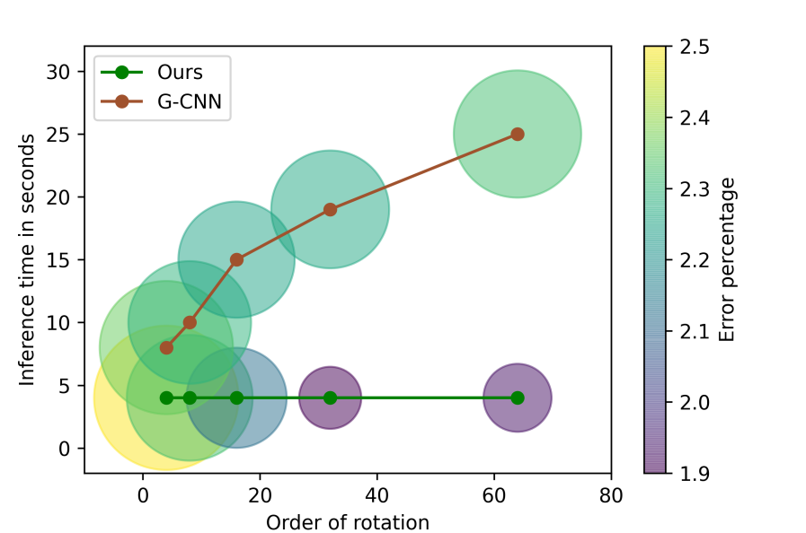
Figure 3: Inference time comparison of our method with G-CNN with increasing order of rotations.

Ablation study

We further seek to understand if learning the canonicalization performs better mainly because a meaningful function is learned, or because this implicitly augments the prediction CNN with rotations during training. We perform an ablation study to investigate this. First, we compare with a CNN trained with random rotation augmentations. Second, we compare with a setup we call CN(pretrained), in which canonicalization is learned along with a CNN prediction network. Then the prediction function is reinitialized and trained from scratch while the canonicalization function is fixed. If a meaningful canonicalization is learned, this setup should perform close to the one where the canonicalization is learned end-to-end. We see from the results of Table 2 that this is the case. The pretrained canonicalization performs almost as close as the end-to-end one and significantly better than data augmentation. We also visualize the canonicalized samples for different canonicalization techniques and order of rotation in Section H.1, confirming that meaningful canonicalization is learned.

Inference time

Next, we compare the inference time of our model with pure G-CNN-based architectures. For this experiment, we take the CNN architecture of our predictor network and replace the convolutions with group convolutions. As increasing the rotation order in G-CNN requires more copies of rotated filters in the lifting layer and more parameters in the subsequent group convolution layers, we decreased the number of channels to keep the number of parameters the same as our model. Figure 3 shows that although G-CNN’s performance is slightly better for the p4 group, increasing the order of discrete rotations improves our model’s performance significantly compared to G-CNN. In addition to performance gain, our model’s inference speed remains more or less constant while encoding invariance to higher-order rotations due to the shallow canonicalization network. This makes our approach more suitable for building equivariance for bigger groups and network architectures.

5.2 $N$-body dynamics prediction

Simulation of physical dynamics is an important class of $E(3)$-equivariant problems due to the symmetry of physical laws under rotations and translations. We evaluate our framework in this setting with the $N$-body dynamics prediction task proposed by (Kipf et al., 2018) and (Fuchs et al., 2020). In this task, the model has to predict the future positions of 5 charged particles interacting with Coulomb force given initial positions and velocities. We use the same version of the dataset and setup as (Satorras et al., 2021).

Table 3: Test MSE for the N-body dynamics prediction task.

Method	MSE
Linear	0.0819
SE(3) Transformer	0.0244
TFN	0.0155
GNN	0.0107
Radial Field	0.0104
EGNN	0.0071
FA-GNN	0.0057
CN-GNN	0.0043 ${\pm}$ 0.0001
CN-GNN-$O(3)$	0.0045 $\pm$ 0.0001
CN-GNN (frozen)	0.0085 $\pm$ 0.0002

For this experiment, our architecture uses a simple 2-layer Vector Neurons version of the Deep Sets architecture for the canonicalization function (Deng et al., 2021; Zaheer et al., 2017a). The prediction function is a 4-layer Graph Neural Network (GNN) with the same hyperparameters as the one used in (Satorras et al., 2021), and (Puny et al., 2022) for a fair comparison. The architecture of the prediction network was, therefore, not optimized. The canonicalization network is much smaller than the prediction GNN, with around 20 times fewer parameters. This allows us to test the hypothesis again that only a simple canonicalization function is necessary to achieve good performance. Section G.2 contains more details on the architecture and training setup.

Results

Table 3 shows that we obtain state-of-the-art results. The improvement with respect to Frame Averaging is significant, showing that learning the canonicalization provides an important advantage. Our approach also does better than all the intrinsically equivariant (or viewpoint-independent) baselines both in accuracy and efficiency. This shows that canonicalization can be used to obtain equivariant models with high generalization abilities without sophisticated architectural choices.

Ablation study

We also test variants of the model. First, we test on a variant of the model where the canonicalization is only learned for the $O\left(3\right)$ part of the transformation and where the translation part is given by the centroid. Since, for this system, all the masses are identical, this is the same as the center of mass of the system. The result is reported in Table 3 as CN-GNN-$O(3)$. We obtain only marginally worse performance compared to the fully trained canonicalization function. This shows that, in this setting, the centroid provides an already suitable canonicalization function, which is expected given the physical soundness of choosing the center of mass as the origin of the reference frame. Since the learned translation canonicalization performs on par with this physically motivated canonicalization, this also validates the method.

The comparison with Frame Averaging is also insightful. PCA-based Frame Averaging can also be motivated from a physical point of view since this method is equivalent to identifying the principal axes using the tensor of inertia. It is, therefore, a physical heuristic for $O\left(3\right)$ canonicalization. By contrast with the translation canonicalization with the centroid, for orthogonal transformations learning, the canonicalization performs significantly better.

Second, we compare with a version of the model where the weights of the canonicalization function are frozen at initialization. This canonicalization still provides $E(n)$-equivariance and, as expected, provides a significant improvement of more than 20% with respect to the GNN prediction function alone. However, the learned canonicalization function provides a close to 50% improvement in performance compared to this fixed canonicalization.

5.3 Point cloud classification and segmentation

We use the ModelNet40 (Wu et al., 2015) and ShapeNet (Chang et al., 2015) datasets for experiments on point clouds. The ModelNet40 dataset consists of 40 classes of 3D models, with a total of 12,311 models. 9,843 models were used for training, and the remaining models were used for testing in the classification task. The ShapeNet dataset was used for part segmentation with the ShapeNet-part subset, which includes 16 categories of objects and more than 30,000 models. In the classification and segmentation task, the train/test rotation setup adhered to the conventions established by (Esteves et al., 2018a) and adopted by (Deng et al., 2021). Three settings were implemented: $z/z$, $z/SO(3)$, and $SO(3)/SO(3)$. The notation $z$ denotes data augmentation with rotations around the z-axis during training, while $SO(3)$ represents arbitrary rotations. The notation $x/y$ denotes that transformation $x$ is applied during training and transformation $y$ is applied during testing.

Table 4: Test classification accuracy of different point cloud models on the ModelNet40 dataset (Wu et al., 2015) in three train/test scenarios. This table is borrowed from (Deng et al., 2021). $z$ here stands for aligned data augmented by random rotations around the vertical axis, and $\mathrm{SO}(3)$ indicates data augmented by random 3D rotations.

Method	$z/z$	$z/\mathrm{SO}(3)$	$\mathrm{SO}(3)/\mathrm{SO}(3)$
Point / mesh inputs
PointNet (Qi et al., 2017a)	85.9	19.6	74.7
DGCNN (Wang et al., 2019)	90.3	33.8	88.6
VN-PointNet	77.5	77.5	77.2
VN-DGCNN	89.5	89.5	90.2
PCNN (Atzmon et al., 2018)	92.3	11.9	85.1
ShellNet (Zhang et al., 2019b)	93.1	19.9	87.8
PointNet++ (Qi et al., 2017b)	91.8	28.4	85.0
PointCNN (Li et al., 2018)	92.5	41.2	84.5
Spherical-CNN (Esteves et al., 2018a)	88.9	76.7	86.9
$a^{3}$S-CNN (Liu et al., 2018)	89.6	87.9	88.7
SFCNN (Rao et al., 2019)	91.4	84.8	90.1
TFN (Thomas et al., 2018)	88.5	85.3	87.6
RI-Conv (Zhang et al., 2019a)	86.5	86.4	86.4
SPHNet (Poulenard et al., 2019)	87.7	86.6	87.6
ClusterNet (Chen et al., 2019)	87.1	87.1	87.1
GC-Conv (Zhang et al., 2020)	89.0	89.1	89.2
RI-Framework (Li et al., 2020)	89.4	89.4	89.3
Ours
CN(frozen)-PointNet	78.9 $\pm$ 2.1	78.7 $\pm$ 2.2	78.4 $\pm$ 2.5
CN(L)-PointNet	79.8 $\pm$ 1.4	79.6 $\pm$ 1.3	79.6 $\pm$ 1.4
CN(NL)-PointNet	79.9 $\pm$ 1.3	79.6 $\pm$ 1.3	79.7 $\pm$ 1.3
CN(frozen)-DGCNN	88.3 $\pm$ 2.1	88.3 $\pm$ 2.1	88.3 $\pm$ 2.1
CN(L)-DGCNN	88.9 $\pm$ 1.8	88.6 $\pm$ 1.9	88.6 $\pm$ 2.0
CN(NL)-DGCNN	88.7 $\pm$ 1.8	88.8 $\pm$ 1.9	90.0 $\pm$ 1.1

We design our Canonicalization Network (CN) using layers from Vector Neurons (Deng et al., 2021), where the final output contains three 3D vectors that are obtained by pooling over the entire point cloud. We then orthonormalize the three vectors using the Gram-Schmidt orthonormalization process to define a 3D ortho-normal coordinate frame or a rotation matrix. We canonicalize the point cloud by acting on it using this rotation matrix. We use a two-layered Vector Neuron network followed by global pooling, which we call CN(NL). To support our hypothesis that the canonicalization function can be inexpressive, we use a single linear layer of Vector neuron followed by pooling and call this model CN(L). Furthermore, to understand the significance of learning canonicalization, we freeze the weights of the CN and call this variant CN(frozen). We use PointNet and DGCNN (Wang et al., 2019) as the prediction networks in our experiments.

Results

Table 4 contains the results of the ShapeNet experiment, showing the classification accuracy for different augmentation strategies during training and evaluation: $z/z$, $z/\mathrm{SO}(3)$, and $\mathrm{SO}(3)/\mathrm{SO}(3)$. Our method, which includes CN(frozen)-PointNet, CN(L)-PointNet, CN(NL)-PointNet, CN(frozen)-DGCNN, CN(L)-DGCNN, and CN(NL)-DGCNN, demonstrates competitive results across all rotation types. We achieve similar results in the ShapeNet part segmentation task as presented in Table 5. In particular, we observe three trends in our results. First, learning canonicalization slightly improves the performance, except in the case where the test point clouds are already aligned ($z/z$ column of Table 4). Second, using shallow linear canonicalization achieves good results. Third, the performance of the prediction network bottlenecks the model’s performance. This verifies our hypothesis that decoupling the equivariance using a simple canonicalization network results in a better and more expressive non-equivariant prediction network to improve the performance of the task while still being equivariant. In Table 6, we also show that the inference time of our algorithm is dominated by the prediction network’s inference time. The overhead of canonicalization is negligible, which makes our method faster than existing methods that modify the entire architecture like Vector Neurons (Deng et al., 2021).

Table 5: ShapeNet part segmentation results. Overall average category mean IoU over 16 categories in two train/test scenarios are reported. $z$ here stands for aligned data augmented by random rotations around the vertical axis, and $\mathrm{SO}(3)$ indicates data augmented by random 3D rotations

Methods	$z/\mathrm{SO}(3)$	$\mathrm{SO}(3)/\mathrm{SO}(3)$
Point / mesh inputs
PointNet (Qi et al., 2017a)	38.0	62.3
DGCNN (Wang et al., 2019)	49.3	78.6
VN-PointNet(Deng et al., 2021)	72.4	72.8
VN-DGCNN(Deng et al., 2021)	81.4	81.4
PointCNN (Li et al., 2018)	34.7	71.4
PointNet++ (Qi et al., 2017b)	48.3	76.7
ShellNet (Zhang et al., 2019b)	47.2	77.1
RI-Conv (Zhang et al., 2019a)	75.3	75.3
TFN (Thomas et al., 2018)	76.8	76.2
GC-Conv (Zhang et al., 2020)	77.2	77.3
RI-Framework (Li et al., 2020)	79.2	79.4
Ours
CN(frozen)-PointNet	72.1 $\pm$ 0.8	72.3 $\pm$ 1.1
CN(L)-PointNet	73.4 $\pm$ 1.2	73.2 $\pm$ 0.9
CN(NL)-PointNet	73.5 $\pm$ 0.8	73.6 $\pm$ 1.1
CN(frozen)-DGCNN	78.1 $\pm$ 1.2	78.2 $\pm$ 1.2
CN(L)-DGCNN	78.5 $\pm$ 1.1	78.3 $\pm$ 1.2
CN(NL)-DGCNN	78.4 $\pm$ 1.0	78.5 $\pm$ 0.9

Table 6: Inference time (in seconds) of the networks for ModelNet40 classification test split in 1 A100 and 8 CPUs with a batch size of 32. Vanilla denotes no modification to the base network, while Vector Neuron and Canonicalization denote that the base network is redesigned/enhanced with them to be equivariant.

Base Network	Vanilla	Vector Neuron	Canonicalization
PointNet	18s	30s	20s
DGCNN	23s	39s	25s

5.4 Discussion

Experimental results have shown the usefulness of our proposed method across different domains: images, $N$-body physical systems and point clouds. This supports the hypothesis that learning a canonicalization tends to perform better than using predefined heuristics to define it. This could be due to a combination of two factors. First, the learned canonicalizations have some consistency and help the prediction network perform the task. This is shown explicitly for our results in the image domain. Second, the process of learning the canonicalization induces an implicit augmentation of the data. This should help the prediction function generalize better and be more robust to potential failings of the canonicalization function. The method therefore combines some of the advantages of data augmentation with exact equivariance.

6 Conclusion

In this work, we propose using a learned canonicalization function to obtain equivariant machine-learning models. These canonicalization functions can conveniently be plugged into existing architectures, resulting in highly expressive models. We have described general approaches to obtain canonicalization functions and specific implementation strategies for the Euclidean group (for images and point clouds) and the symmetric group.

We performed experimental studies in the image, dynamical systems and point cloud domains to test our hypotheses. First, we show that our approach achieves comparable or better performance than baselines on invariant tasks. Importantly, learning the canonical network is a better approach than using a fixed mapping, either a frozen neural network or a heuristic approach. Our results also show that the canonicalization function can be realized with a shallow equivariant network without hindering performance. Finally, we show that this approach reduces inference time and is more suitable for bigger groups than G-CNNs on images.

One limitation of our method is that there are no guarantees that the canonicalization function is smooth. This may be detrimental to generalization as small changes in the input could lead to large variations in the input to the prediction function. Another limitation could arise in domains in which semantic content is lacking to identify a meaningful canonicalization, for example, some types of astronomical images or biological images.

Multiple extensions of this framework are possible. Future work could include experimentation on canonicalization for the symmetric group. Other ways to build canonicalization functions could also be investigated, such as using steerable networks for images. The function would output an orientation fibre that transforms by the irreducible representation of the special orthogonal group. Understanding how design choices for canonicalization functions (for example, the subgroup $K$) affect downstream performance could also be a fruitful research direction. Finally, making large pretrained architectures equivariant using this framework could be an exciting extension.

Appendix

Appendix A Symmetric inputs and relaxed equivariance

An input $\mathbf{x}\in\mathcal{X}$ is symmetric if its stabilizer subgroup $G_{\mathbf{x}}=\left\{g\in G\mid\rho\left(g\right)\mathbf{x}=\mathbf{x}\right\}$ is non-trivial. In other words, symmetric inputs are fixed by multiple group elements.

Given any $g_{1},g_{2}\in G$, we have $\rho\left(g_{1}\right)\mathbf{x}=\rho\left(g_{2}\right)\mathbf{x}$ if and only if $g_{1}$ and $g_{2}$ are part of the same coset for the stabilizer, e.g. $g_{1},g_{2}\in gG_{\mathbf{x}}$. This follows from the well-known relation between orbits and stabilizers.

Symmetric inputs are problematic when using the standard definition of equivariance for the canonicalization function because for $g_{1},g_{2}\in gG_{\mathbf{x}}$, we have

$$h\left(\rho\left(g_{1}\right)\mathbf{x}\right)=h\left(\rho\left(g_{2}\right)\mathbf{x}\right),$$ (11)

$$\rho\left(g_{1}\right)h\left(\mathbf{x}\right)=\rho\left(g_{2}\right)h\left(\mathbf{x}\right).$$ (12)

If $g_{1}\neq g_{2}$, there cannot exist a $h\left(\mathbf{x}\right)\in\rho\left(G\right)$ such that the last equality is satisfied.

We define a relaxed version of equivariance to address this.

Definition A.1 (Relaxed equivariance).

Given group representations $\rho:G\to\mathrm{GL}\left(\mathcal{X}\right)$ and $\rho^{\prime}:G\to\mathrm{GL}\left(\mathcal{Y}\right)$, a function $h:\mathcal{X}\to\mathcal{Y}$ satisfies relaxed equivariance if $\forall g_{1},\mathbf{x}\in G\times X$ there exists a $g_{2}\in g_{1}G_{\mathbf{x}}$ such that

$$h\left(\rho\left(g_{1}\right)\mathbf{x}\right)=\rho^{\prime}\left(g_{2}\right)h\left(\mathbf{x}\right).$$ (13)

Note that relaxed invariance coincides with standard invariance. It is possible to build canonicalization functions that satisfy this condition as we show in the next appendix.

We also prove the following important result.

Theorem A.2.

A function $\phi$ defined by Equation 2 satisfies the relaxed equivariance condition if the canonicalization function $h$ satisfies the relaxed equivariance condition.

Proof.

We start with:

$$\mbox{\boldmath$\phi$}\left(\rho\left(g_{1}\right)\mathbf{x}\right)=h^{\prime}\left(\rho\left(g_{1}\right)\mathbf{x}\right)\mathbf{f}\left(h\left(\rho\left(g_{1}\right)\mathbf{x}\right)^{-1}\rho\left(g_{1}\right)\mathbf{x}\right)$$ (14)

Using the definition of relaxed equivariance A.1, we obtain the following, where $g_{2}\in g_{1}G_{\mathbf{x}}$ :

$$\mbox{\boldmath$\phi$}\left(\rho\left(g_{1}\right)\mathbf{x}\right)=\rho^{\prime}\left(g_{2}\right)h^{\prime}\left(\mathbf{x}\right)\mathbf{f}\left(h\left(\mathbf{x}\right)^{-1}\rho\left(g_{2}\right)^{-1}\rho\left(g_{1}\right)\mathbf{x}\right)$$ (15)

$$\mbox{\boldmath$\phi$}\left(\rho\left(g_{1}\right)\mathbf{x}\right)=\rho^{\prime}\left(g_{2}\right)h^{\prime}\left(\mathbf{x}\right)\mathbf{f}\left(h\left(\mathbf{x}\right)^{-1}\rho\left({g_{2}}^{-1}g_{1}\right)\mathbf{x}\right)$$ (16)

Using the fact that ${g_{2}}^{-1}g_{1}\in G_{\mathbf{x}}$,

$$\mbox{\boldmath$\phi$}\left(\rho\left(g_{1}\right)\mathbf{x}\right)=\rho^{\prime}\left(g_{2}\right)h^{\prime}\left(\mathbf{x}\right)\mathbf{f}\left(h\left(\mathbf{x}\right)^{-1}\mathbf{x}\right)$$ (17)

$$\mbox{\boldmath$\phi$}\left(\rho\left(g_{1}\right)\mathbf{x}\right)=\rho^{\prime}\left(g_{2}\right)\mbox{\boldmath$\phi$}\left(\mathbf{x}\right)$$ (18)

Therefore, $\phi$ satisfies relaxed equivariance and this completes the proof. ∎

We provide more discussion on relaxed equivariance. Standard equivariance requires that symmetric inputs are mapped to symmetric inputs. This is a limitation in many situations others than canonicalization that relxed equivariance allows to bypass.

Aside from its importance for canonicalization, relaxed equivariance is thus a very useful concept in itself. It generalizes the idea of multiset-equivariance from Zhang et al. (2022) to arbitrary groups. The relaxation captures the idea of equivariance up to symmetry and solves the inability of equivariant functions to break symmetry (Smidt et al., 2021; Satorras et al., 2021). It should therefore be more desirable than standard equivariance in many instances. For example, in physics, it allows to model symmetry breaking phenomenons or in graph representation learning, it allows to map nodes that are part of the same orbit to different embeddings.

The fact that we obtain relaxed equivariance for the canonicalized function is therefore a feature rather than a bug. This captures the desideratum that a function should be able to output asymmetric outputs from symmetric inputs.

Figure 4 shows simple examples of function that cannot be approximated by equivariant functions. In Figure 4(a) assuming that the input is an image with uniform pixel values (fully symmetric), a translation equivariant function cannot output any image with non-uniform pixel values. In Figure 4(b), the input could be the symmetric graph of a molecule, with nodes $1$ and $3$ part of the same orbit. It is impossible for a permutation equivariant function to give different outputs (for example charge polarization) for these nodes. Yet, it is clear that in many situations such functions should not be excluded.

(a) Translation or rotation equivariant function on images

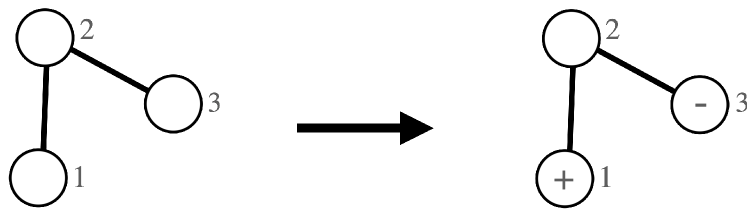
(b) Permutation equivariant function on graphs

Figure 4: Example of task that cannot be performed by equivariant functions.

Appendix B Optimization approach to canonicalization

In this appendix, we provide a more formal description of canonicalization functions obtained with the optimization approach of section 4.

We prove a theorem providing a sufficient condition for a canonicalization function to satisfy the relaxed equivariance condition A.1.

Theorem B.1.

Let $h\left(\mathbf{x}\right)\in\operatornamewithlimits{arg\,min}_{\rho\left(g\right)\in\rho\left(G\right)}s\left(\rho\left(g\right),\mathbf{x}\right)$ for some $s:\rho\left(G\right)\times\mathcal{X}\to\mathbb{R}$. If the conditions

1. $\forall g,g_{1}\in G,\forall\mathbf{x}\in\mathcal{X},\ s\left(\rho\left(g\right),\rho\left(g_{1}\right)\mathbf{x}\right)=s\left(\rho\left(g_{1}\right)^{-1}\rho\left(g\right),\mathbf{x}\right)$

2. $\forall\mathbf{x},\exists g_{1}\in G$, such that $\operatornamewithlimits{arg\,min}_{\rho\left(g\right)\in\rho\left(G\right)}s\left(\rho\left(g\right),\mathbf{x}\right)\subseteq\rho\left(G_{\mathbf{x}}g_{1}\right)$ where $G_{\mathbf{x}}$ is the stabilizer subgroup of $\mathbf{x}$

are satisfied then $h\left(\mathbf{x}\right)$ satisfies the relaxed equivariance condition A.1.

Proof.

Let us introduce the shorthand notation $\rho\left(H_{\mathbf{x}}\right)=\operatornamewithlimits{arg\,min}_{\rho\left(g\right)\in\rho\left(G\right)}s\left(\rho\left(g\right),\mathbf{x}\right)$. We define $H_{\mathbf{x}}$ as a subset of $G$ such that its image under $\rho$ is the argmin.

We have

$$\rho\left(H_{\rho\left(g_{1}\right)\mathbf{x}}\right)=\operatornamewithlimits{arg\,min}_{\rho\left(g\right)\in\rho\left(G\right)}s\left(\rho\left(g\right),\rho\left(g_{1}\right)\mathbf{x}\right)$$ (19)

Using condition 1, we have

$$\rho\left(H_{\rho\left(g_{1}\right)\mathbf{x}}\right)=\operatornamewithlimits{arg\,min}_{\rho\left(g\right)\in\rho\left(G\right)}s\left(\rho\left(g_{1}\right)^{-1}\rho\left(g\right),\mathbf{x}\right)$$ (20)

We can use the fact that left multiplication by $\rho\left(g_{1}\right)$ of the elements of $\rho\left(H_{\mathbf{x}}\right)$ will give the argmin in the previous equation. Therefore we have $\rho\left(H_{\rho\left(g_{1}\right)\mathbf{x}}\right)=\rho\left(g_{1}H_{\mathbf{x}}\right)$.

Next, using condition 2, there exists a $g_{3}\in G$ such that $\rho\left(H_{\mathbf{x}}\right)\subseteq\rho\left(G_{\mathbf{x}}g_{3}\right)$ and $\rho\left(g_{1}H_{\mathbf{x}}\right)\subseteq\rho\left(g_{1}G_{\mathbf{x}}g_{3}\right)$.

Finally, we can show that for any $h\left(\mathbf{x}\right)\in\rho\left(G_{\mathbf{x}}g_{3}\right)$ and $h\left(\rho\left(g_{1}\right)\mathbf{x}\right)\in\rho\left(g_{1}G_{\mathbf{x}}g_{3}\right)$, there is a $g_{2}\in g_{1}G_{\mathbf{x}}$ such that

$$h\left(\rho\left(g_{1}\right)\mathbf{x}\right)=\rho\left(g_{2}\right)h\left(\mathbf{x}\right)$$ (21)

The left-hand side can be expressed as $h\left(\rho\left(g_{1}\right)\mathbf{x}\right)=\rho\left(g_{1}\right)h^{\prime}\left(\mathbf{x}\right)$, where $h^{\prime}\left(\mathbf{x}\right)\in\rho\left(G_{\mathbf{x}}g_{3}\right)$. We then find

$$\rho\left(g_{2}\right)=\rho\left(g_{1}\right)h^{\prime}\left(\mathbf{x}\right)h\left(\mathbf{x}\right)^{-1}$$ (22)

Since $h\left(\mathbf{x}\right)$ and $h^{\prime}\left(\mathbf{x}\right)$ are part of the same coset of the stabilizer, $h^{\prime}\left(\mathbf{x}\right)h\left(\mathbf{x}\right)^{-1}$ must be part of the stabilizer. This completes the proof.

∎

Now let us discuss how the conditions of Theorem B.1 can be met.

One way to satisfy the first condition is by using an equivariant function. Notice that the function $s:\rho\left(G\right)\times\mathcal{X}\to\mathbb{R}$ can be reinterpreted as $s:\mathcal{X}\to\mathbb{R}^{\rho\left(G\right)}$. Therefore $s$ can be seen as a function of the input outputting a vector for which the components index the group representation. This vector should transform equivariantly for condition 1 to be satisfied, e.g. $s\left(\rho\left(g_{1}\right)\mathbf{x}\right)_{\rho\left(g\right)}=s\left(\mathbf{x}\right)_{\rho\left(g\right)_{1}^{-1}\rho\left(g\right)}$.

Another way to satisfy condition 1 is to define $s\left(\rho\left(g\right),\mathbf{x}\right)=u\left(\rho\left(g\right)^{-1}\mathbf{x}\right)$. It is easy to verify that this will indeed satisfy the condition.

Finally, as stated in the main text, condition 2 amounts to having a unique minimum in each orbit up an element of the stabilizer of the input. We will not show formally how this can be satisfied, but this is not expected to be a problem in practice. We conjecture that under weak assumptions, following the result of (Cox, 2020), neural network functions can be obtained such that this condition is satisfied almost surely. In addition, for continuous groups, optimization can be made easier by making these neural network functions convex, which can be done using the framework of ICNN (Amos et al., 2017).

Appendix C Proof of Theorem 3.1

We prove Theorem 3.1 which shows equivariance for a general subgroup $K$.

Proof.

We have

$$\mbox{\boldmath$\phi$}\left(\rho\left(g\right)\mathbf{x}\right)=h^{\prime}\left(\rho\left(g\right)\mathbf{x}\right)\mathbf{f}\left(h\left(\rho\left(g\right)\mathbf{x}\right)^{-1}\rho\left(g\right)\mathbf{x}\right)$$ (23)

If equation 3 is satisfied, then $\forall\ g,\mathbf{x}\in G\times\mathcal{X}$ there is a $k\in K$ such that

$$\mbox{\boldmath$\phi$}\left(\rho\left(g\right)\mathbf{x}\right) =\rho^{\prime}\left(g\right)h^{\prime}\left(\mathbf{x}\right)\rho^{\prime}\left(k\right)\mathbf{f}\left(\left[\rho\left(g\right)h\left(\mathbf{x}\right)\rho\left(k\right)^{-1}\right]^{-1}\rho\left(g\right)\mathbf{x}\right)$$ (24)

$$\mbox{\boldmath$\phi$}\left(\rho\left(g\right)\mathbf{x}\right) =\rho^{\prime}\left(g\right)h^{\prime}\left(\mathbf{x}\right)\rho^{\prime}\left(k\right)\mathbf{f}\left({\rho\left(k\right)^{-1}h\left(\mathbf{x}\right)^{-1}\rho\left(g\right)^{-1}}\rho\left(g\right)\mathbf{x}\right)$$ (25)

Using the $K$-equivariance of $\mathbf{f}$, we obtain

$$\mbox{\boldmath$\phi$}\left(\rho\left(g\right)\mathbf{x}\right) =\rho^{\prime}\left(g\right)h^{\prime}\left(\mathbf{x}\right)\rho^{\prime}\left(k\right)\rho^{\prime}\left(k\right)^{-1}\mathbf{f}\left({h\left(\mathbf{x}\right)^{-1}}\mathbf{x}\right)$$ (26)

$$\mbox{\boldmath$\phi$}\left(\rho\left(g\right)\mathbf{x}\right) =\rho^{\prime}\left(g\right)h^{\prime}\left(\mathbf{x}\right)\mathbf{f}\left({h\left(\mathbf{x}\right)^{-1}}\mathbf{x}\right)$$ (27)

∎

Appendix D Proof of Theorem 3.2

Proof.

We consider the special case where $K$ is a normal subgroup of $G$ such that the group can be taken to be isomorphic to a semidirect product $G\simeq K\rtimes J$. Then, group elements can be written as $g=\left(k,j\right)$, where $k\in K$ and $j\in J$. The product is defined as $g_{1}g_{2}=\left(k_{1},j_{1}\right)\left(k_{2},j_{2}\right)=\left(k_{1}\varphi\left[j_{1}\right]\left(k_{2}\right),j_{1}j_{2}\right)$, where $\varphi:J\to\mathrm{Aut}\left(K\right)$ is a group homomorphism. Setting $k_{2}=e$ and $j_{1}=e$, we get any group element as $\left(k_{1},e\right)\left(e,j_{2}\right)=\left(k_{1},j_{2}\right)$.

If the canonicalization function is $J$-equivariant and $K$-invariant, we have

$$h\left(\rho\left(k,j\right)\mathbf{x}\right) =h\left(\rho\left(k,e\right)\rho\left(e,j\right)\mathbf{x}\right)$$ (28)

$$h\left(\rho\left(k,j\right)\mathbf{x}\right) =\rho\left(e,j\right)h\left(\mathbf{x}\right)$$ (29)

We then show that there is a $k^{\prime}\in K$ such that equation 3 is satisfied. Multiplying by $\rho\left(e\right)=\rho\left(k,e\right)\rho\left(e,j\right)h\left(\mathbf{x}\right)h\left(\mathbf{x}\right)^{-1}\rho\left(e,j\right)^{-1}\rho\left(k,e\right)^{-1}$ on the left, we have

$$\rho\left(e,j\right)h\left(\mathbf{x}\right) =\rho\left(k,e\right)\rho\left(e,j\right)h\left(\mathbf{x}\right)h\left(\mathbf{x}\right)^{-1}\rho\left(e,j\right)^{-1}\rho\left(k,e\right)^{-1}\rho\left(e,j\right)h\left(\mathbf{x}\right)$$ (30)

Using the fact that conjugation of an element of $K$ by an element of $G$ preserves $K$ membership, we define $\rho\left(k^{\prime},e\right)=h\left(\mathbf{x}\right)^{-1}\rho\left(e,j\right)^{-1}\rho\left(k,e\right)^{-1}\rho\left(e,j\right)h\left(\mathbf{x}\right)$

$$\rho\left(e,j\right)h\left(\mathbf{x}\right) =\rho\left(k,e\right)\rho\left(e,j\right)h\left(\mathbf{x}\right)\rho\left(k^{\prime},e\right)$$ (31)

which shows that equation 3 is satisfied.

Finally, we show that in this case, the image of $h$ can be chosen to be $\rho\left(J\right)$. We first remark that in each orbit $\mathcal{X}/G$ of the group action, the canonical sample $\hat{\mathbf{x}}$ can be obtained from any orbit member $\mathbf{x}$, as $\hat{\mathbf{x}}=h\left(\mathbf{x}\right)^{-1}\mathbf{x}$. For the canonical sample, we must have a $k\in K$ such that

$$h\left(h\left(\mathbf{x}\right)^{-1}\mathbf{x}\right)=h\left(\mathbf{x}\right)^{-1}h\left(\mathbf{x}\right)\rho\left(k,e\right)$$ (32)

If we impose $k=e$ to satisfy this condition, we have $h\left(\hat{\mathbf{x}}\right)=\rho\left(e,e\right)$.

Since any orbit member can conversely be written as $\mathbf{x}=\rho\left(k,j\right)\hat{\mathbf{x}}$ for some $k\in K$ and $j\in J$, if the canonicalization function is $J$-equivariant and $K$-invariant, we have

$$h\left(\mathbf{x}\right) =h\left(\rho\left(k,j\right)\hat{\mathbf{x}}\right)$$ (33)

$$h\left(\mathbf{x}\right) =\rho\left(e,j\right)h\left(\hat{\mathbf{x}}\right)$$ (34)

$$h\left(\mathbf{x}\right) =\rho\left(e,j\right)$$ (35)

which completes the proof. ∎

Appendix E Proof of Theorem 3.3

Proof.

The proof is inspired by the symmetrization approach of (Yarotsky, 2022) and (Puny et al., 2022).

We first claim that given a compact set $\mathcal{K}\subseteq\mathcal{X}$, the set $\widetilde{\mathcal{K}}=\left\{h\left(\mathbf{x}\right)^{-1}\mathbf{x}:\mathbf{x}\in\mathcal{K}\right\}$ is also compact.

To see this, we notice that the map $\mathbf{x}\mapsto h\left(\mathbf{x}\right)^{-1}$ is continuous, since it is the composition of the continuous function $h$ and of the inverse map $L\mapsto L^{-1}$. We use the fact that linear operators on $\mathcal{X}$ form a Banach algebra and that the inverse map on Banach algebras is continuous. The map $\mathbf{x}\mapsto h\left(\mathbf{x}\right)^{-1}$ is then composed with the evaluation map $\left(L,\mathbf{x}\right)\mapsto L\mathbf{x}$. The latter is continuous since $\mathcal{X}$ is locally compact and Hausdorff.

Then, let $\psi$ be an arbitrary $G$-equivariant function, and $\phi$ be defined by equation 2. We have

$$\norm{\mbox{\boldmath$\psi$}\left(\mathbf{x}\right)-\mbox{\boldmath$\phi$}\left(\mathbf{x}\right)} =\norm{\mbox{\boldmath$\psi$}\left(\mathbf{x}\right)-h^{\prime}\left(\mathbf{x}\right)\mathbf{f}\left(h\left(\mathbf{x}\right)^{-1}\mathbf{x}\right)}.$$ (36)

By the equivariance of $\psi$, we obtain

$$\norm{\mbox{\boldmath$\psi$}\left(\mathbf{x}\right)-\mbox{\boldmath$\phi$}\left(\mathbf{x}\right)} =\norm{h^{\prime}\left(\mathbf{x}\right)\mbox{\boldmath$\psi$}\left(h\left(\mathbf{x}\right)^{-1}\mathbf{x}\right)-h^{\prime}\left(\mathbf{x}\right)\mathbf{f}\left(h\left(\mathbf{x}\right)^{-1}\mathbf{x}\right)}.$$ (37)

We have that $\norm{h^{\prime}\left(\mathbf{x}\right)}$ is bounded on $\mathcal{K}$ from continuity of $h^{\prime}$ and of the induced operator norm. We therefore define $c=\sup_{\mathbf{x}\in\mathcal{K}}\norm{h^{\prime}\left(\mathbf{x}\right)}>0$ and obtain

$$\norm{\mbox{\boldmath$\psi$}\left(\mathbf{x}\right)-\mbox{\boldmath$\phi$}\left(\mathbf{x}\right)} \leq\norm{h\left(\mathbf{x}\right)}\norm{\mbox{\boldmath$\psi$}\left(h\left(\mathbf{x}\right)^{-1}\mathbf{x}\right)-\mathbf{f}\left(h\left(\mathbf{x}\right)^{-1}\mathbf{x}\right)},$$ (38)

$$\norm{\mbox{\boldmath$\psi$}\left(\mathbf{x}\right)-\mbox{\boldmath$\phi$}\left(\mathbf{x}\right)} \leq c\norm{\mbox{\boldmath$\psi$}\left(h\left(\mathbf{x}\right)^{-1}\mathbf{x}\right)-\mathbf{f}\left(h\left(\mathbf{x}\right)^{-1}\mathbf{x}\right)},\ \forall\ \mathbf{x}\in\mathcal{K}.$$ (39)

Using the assumption that $\mathbf{f}$ is a universal approximator of $K$-equivariant functions, we know that it is also a universal approximator of $G$-equivariant functions. We therefore have for any $\delta>0$,

$$\norm{\mbox{\boldmath$\psi$}\left(\tilde{\mathbf{x}}\right)-\mathbf{f}\left(\tilde{\mathbf{x}}\right)}\leq\delta,\ \forall\ \tilde{\mathbf{x}}\in\widetilde{\mathcal{K}}.$$ (40)

In particular, we consider $\delta=\epsilon/c$. Replacing in Equation 39, we obtain the desired result

$$\norm{\mbox{\boldmath$\psi$}\left(\mathbf{x}\right)-\mbox{\boldmath$\phi$}\left(\mathbf{x}\right)} \leq\epsilon,\ \forall\ \mathbf{x}\in\mathcal{K}.$$ (41)

∎

Appendix F Proof of Theorem 5

Theorem F.1.

The Gram-Schmidt process is $O\left(n\right)$-equivariant.

Proof.

Given $n$ linearly independent input vectors $\mathbf{v}_{1},\dots,\mathbf{v}_{n}$, the Gram-Schmidt process first produces the orthogonal vectors $\mathbf{u}_{1},\dots,\mathbf{u}_{n}$, with

$$\mathbf{u}_{i}\left(\mathbf{v}_{1},\dots,\mathbf{v}_{n}\right)=\mathbf{v}_{i}-\sum_{j=1}^{i-1}\frac{\mathbf{u}_{j}\cdot\mathbf{v}_{i}}{\norm{\mathbf{u}_{j}}^{2}}\mathbf{u}_{j}$$ (42)

The orthonormal basis $\mathbf{e}_{1},\dots,\mathbf{e}_{n}$ is then given by

$$\mathbf{e}_{i}\left(\mathbf{v}_{1},\dots,\mathbf{v}_{n}\right)=\frac{\mathbf{u}_{i}}{\norm{\mathbf{u}_{i}}}$$ (43)

We wish to prove that $\forall i\leq n,\mathbf{O}\in O\left(n\right)$, we have

$$\mathbf{e}_{i}\left(\mathbf{O}\mathbf{v}_{1},\dots,\mathbf{O}\mathbf{v}_{n}\right)=\mathbf{O}\mathbf{e}_{i}\left(\mathbf{v}_{1},\dots,\mathbf{v}_{n}\right)$$ (44)

We first prove equivariance of (42) by strong induction. Consider the base case with $i=1$. We have $\mathbf{u}_{1}\left(\mathbf{v}_{1},\dots,\mathbf{v}_{n}\right)=\mathbf{v}_{1}$, which is trivially equivariant. Then, we make the induction hypothesis that (42) is equivariant for $1\leq i\leq k$. We can show that this implies equivariance for $i=k+1$. We have

$$\mathbf{u}_{k+1}\left(\mathbf{v}_{1},\dots,\mathbf{v}_{n}\right)=\mathbf{v}_{k+1}-\sum_{j=1}^{k}\frac{\mathbf{u}_{j}\cdot\mathbf{v}_{k+1}}{\norm{\mathbf{u}_{j}}^{2}}\mathbf{u}_{j}$$ (45)

Using the induction hypothesis, we obtain

$$\mathbf{u}_{k+1}\left(\mathbf{O}\mathbf{v}_{1},\dots,\mathbf{O}\mathbf{v}_{n}\right)=\mathbf{O}\mathbf{v}_{k+1}-\sum_{j=1}^{k}\frac{\mathbf{O}\mathbf{u}_{j}\cdot\mathbf{O}\mathbf{v}_{k+1}}{\norm{\mathbf{O}\mathbf{u}_{j}}^{2}}\mathbf{O}\mathbf{u}_{j}$$ (46)

Since the dot product and the Euclidean norm are $O\left(n\right)$-invariant, we obtain

$$\mathbf{u}_{k+1}\left(\mathbf{O}\mathbf{v}_{1},\dots,\mathbf{O}\mathbf{v}_{n}\right)=\mathbf{O}\mathbf{v}_{k+1}-\sum_{j=1}^{k}\frac{\mathbf{u}_{j}\cdot\mathbf{v}_{k+1}}{\norm{\mathbf{u}_{j}}^{2}}\mathbf{O}\mathbf{u}_{j}$$ (47)

$$\mathbf{u}_{k+1}\left(\mathbf{O}\mathbf{v}_{1},\dots,\mathbf{O}\mathbf{v}_{n}\right)=\mathbf{O}\left(\mathbf{v}_{k+1}-\sum_{j=1}^{k}\frac{\mathbf{u}_{j}\cdot\mathbf{v}_{k+1}}{\norm{\mathbf{u}_{j}}^{2}}\mathbf{u}_{j}\right)$$ (48)

which completes the induction.

We finally see that by $O\left(n\right)$-invariance of the Euclidean norm, (43) is also equivariant. Since the composition of equivariant functions is equivariant, we find that the Gram-Schmidt process is equivariant and this completes the proof.

∎

Appendix G Implementation details

G.1 Image classification experiments

Training details.

In all our image experiments, we train the models by minimizing the cross entropy loss for 100 epochs using Adam (Kingma & Ba, 2014) with a learning rate of 0.001. We perform early stopping based on the classification performance of the validation dataset with a patience of 20 epochs.

CNN architecture.

For CNN (base), we choose an architecture with 7 layers where layer 1 to 3 has 32, 4 to 6 has 64, and layer 7 has 128 channels, respectively. Instead of pooling, we use convolution filters of size $5\times 5$ with a stride 2 at layers 4 and 7. The remaining convolutions have filters of size $3\times 3$ and stride 1. All the layers are followed by batch-norm (Ioffe & Szegedy, 2015) and ReLU activation with dropout(p=0.4) only at layers 4 and 7.

G-CNN architecture.

We took the same CNN architecture as above and replaced the standard convolutions with group convolutions (Cohen & Welling, 2016b).

Optimization approach.

For the energy function $E$, the image is transformed to a point cloud and fed into a Deep Sets (Zaheer et al., 2017b) architecture. Then, $E$ is optimized by 5-steps of gradient descent (learning rate 0.1) using implicit differentiation.

G.2 $N$-body dynamics prediction experiments

Training details.

We train on mean square error (MSE) loss between predicted and ground truth using the Adam optimizer. We train for 10.000 epochs and use early stopping. We use weight decay $10^{-8}$ and dropout in the canonicalization function with $p=0.5$.

Canonicalization network architecture.

We use a Vector Neurons version of the Deep Sets architecture for the canonicalization network in this task. The network has two layers with hidden dimension size of 32.

Prediction network architecture.

The GNN prediction network uses the same architecture as (Satorras et al., 2021).

G.3 Point Cloud Classification and Segmentation experiments

Training Details

We use cross entropy loss and Stochastic Gradient Descent (SGD) optimizer to train the network for $200$ epochs in all of our pointcloud experiments. We use a initial learning rate of $0.1$ and cosine annealing schedule with an end learning rate of $0.001$.

Canonicalization network architecture.

We design our Canonicalization Network (CN) using layers from Vector Neurons (Deng et al., 2021), where the final output contains three 3D vectors that are obtained by pooling over the entire point cloud. We then orthonormalize the three vectors using the Gram-Schmidt orthonormalization process to define a 3D ortho-normal coordinate frame or a rotation matrix.

Prediction network architecture.

We use PointNet and DGCNN (Wang et al., 2019) as the prediction networks in our experiments.

Appendix H Additional results

H.1 Image classification

Table 7: Impact of the number of layers in canonicalization function network and order of the discrete rotations to which it is equivariant on the performance.

#lyrs Order of the discrete rotation group p4 p8 p16 p32 p64 1 2.52 $\pm$ 0.12 2.37 $\pm$ 0.09 2.20 $\pm$ 0.08 2.05 $\pm$ 0.15 2.01 $\pm$ 0.09 2 2.44 $\pm$ 0.06 2.31 $\pm$ 0.05 2.16 $\pm$ 0.09 2.00 $\pm$ 0.07 2.02 $\pm$ 0.12 3 2.41 $\pm$ 0.11 2.28 $\pm$ 0.09 2.11 $\pm$ 0.06 1.98 $\pm$ 0.09 1.99 $\pm$ 0.10

First, we vary the number of layers of the canonicalization network and the number of rotations it is equivariant to. For this, we extend the layers of G-CNN to any arbitrary rotations. As we noticed that using a larger filter leads to better performance for higher order rotations, we stick to architecture with a lifting layer with image-sized filters followed by $1\times 1$ filters. From Table 6, we notice that adding equivariance to higher order rotation in the canonicalization function leads to significant performance improvement compared to adding more layers. Figure 5 shows the canonical orientation resulting from the learnt canonicalization function with a single lifting layer on 90 randomly sampled images of class 7 from the test dataset. This suggests that a shallow network is sufficient to achieve good results with a sufficiently high order of discrete rotations. For p64, we see that all the similar-looking samples are aligned in one particular orientation. In contrast, although techniques like PCA or freezing parameters of the canonicalization function find the correct canonicalization function for simple digits like 1, they struggle to find stable mappings for more complicated digits like $7$.

(a) Original

(b) p4

(c) p8

(d) p16

(e) p32

(f) p64

(g) p64 (frozen)

(h) PCA

(i) Original

(j) p4

(k) p8

(l) p16

(m) p32

(n) p64

(o) p64 (frozen)

(p) PCA

Figure 5: Canonicalized images from different canonicalization functions for digit 7.

Appendix I Algorithm for Image Inputs

Algorithm 1 Differentiable Canonicalization for Image Inputs

⬇

import torch.nn.functional as F

import kornia as K

def get_canonicalized_images(images, fibre_features, use_reflection=True):

"""

␣␣␣␣images:␣Tensor␣with␣shape␣(batch_size,␣in_channels,␣height,␣width)

␣␣␣␣fibres_features:␣Tensor␣with␣shape:␣(batch_size,␣num_group_elements)

␣␣␣␣use_reflection:␣Boolean

␣␣␣␣:return:␣(batch_size,␣in_channels,␣height,␣width)

␣␣␣␣"""

num_group_elements = fibre_features.shape[-1]

num_rotations = num_group_elements // 2 if use_reflection else num_group_elements

fibre_features_one_hot = F.one_hot(

torch.argmax(fibre_features, dim=-1),

num_group_elements

).float()

fibre_features_soft = F.softmax(fibre_features, dim=-1)

ref_angles = torch.linspace(0., 360., num_rotations+1)[:num_rotations]

if use_reflection:

ref_angles = torch.cat([ref_angles, ref_angles], dim=0)

angles = torch.sum((

fibre_features_one_hot + fibre_features_soft - fibre_features_soft.detach()

) * ref_angles, dim=-1)

if use_reflection:

reflect_one_hot = torch.cat(

[torch.zeros(num_rotations), torch.ones(num_rotations)]

, dim=0)

reflect_indicator = torch.sum((

fibre_features_one_hot + fibre_features_soft - fibre_features_soft.detach()

) * reflect_one_hot, dim=-1)

images_reflected = K.geometry.hflip(images)

reflect_indicator = reflect_indicator[:,None,None,None]

images = (1 - reflect_indicator) * images + reflect_indicator * images_reflected

return K.geometry.rotate(images, -angles)

# Use a shallow G-CNN as a canonicalization_network

feature_map = canonicalization_network(images)

# feature_map shape: (batch_size, num_channels, num_group_elements, height, width)

fibre_features = feature_map.mean(dim=(1, 3, 4))

# fibre_features shape: (batch_size, num_group_elements)

canonicalized_images = get_canonicalized_images(images, fibre_featuresr)

References

- Amos et al. (2017) Amos, B., Xu, L., and Kolter, J. Z. Input convex neural networks. In Precup, D. and Teh, Y. W. (eds.), Proceedings of the 34th International Conference on Machine Learning, volume 70 of Proceedings of Machine Learning Research, pp. 146–155. PMLR, 06–11 Aug 2017.
- Atzmon et al. (2018) Atzmon, M., Maron, H., and Lipman, Y. Point convolutional neural networks by extension operators. arXiv preprint arXiv:1803.10091, 2018.
- Bengio et al. (2013) Bengio, Y., Léonard, N., and Courville, A. Estimating or propagating gradients through stochastic neurons for conditional computation. arXiv preprint arXiv:1308.3432, 2013.
- Benton et al. (2020) Benton, G., Finzi, M., Izmailov, P., and Wilson, A. G. Learning invariances in neural networks from training data. Advances in neural information processing systems, 33:17605–17616, 2020.
- Bloem-Reddy & Teh (2020) Bloem-Reddy, B. and Teh, Y. W. Probabilistic symmetries and invariant neural networks. The Journal of Machine Learning Research, 21(1):3535–3595, 2020.
- Blondel et al. (2018) Blondel, M., Seguy, V., and Rolet, A. Smooth and sparse optimal transport. In International conference on artificial intelligence and statistics, pp. 880–889. PMLR, 2018.
- Blondel et al. (2020) Blondel, M., Teboul, O., Berthet, Q., and Djolonga, J. Fast differentiable sorting and ranking. In III, H. D. and Singh, A. (eds.), Proceedings of the 37th International Conference on Machine Learning, volume 119 of Proceedings of Machine Learning Research, pp. 950–959. PMLR, 13–18 Jul 2020. URL https://proceedings.mlr.press/v119/blondel20a.html.
- Blondel et al. (2022) Blondel, M., Berthet, Q., marco cuturi, Frostig, R., Hoyer, S., Llinares-López, F., Pedregosa, F., and Vert, J.-P. Efficient and modular implicit differentiation, 2022. URL https://openreview.net/forum?id=TQ75Md-FqQp.
- Bogatskiy et al. (2022) Bogatskiy, A., Ganguly, S., Kipf, T., Kondor, R., Miller, D. W., Murnane, D., Offermann, J. T., Pettee, M., Shanahan, P., Shimmin, C., et al. Symmetry group equivariant architectures for physics. arXiv preprint arXiv:2203.06153, 2022.
- Bronstein et al. (2021) Bronstein, M. M., Bruna, J., Cohen, T., and Veliković, P. Geometric deep learning: Grids, groups, graphs, geodesics, and gauges. arXiv preprint arXiv:2104.13478, 2021.
- Carpenter & Eisenberg (1978) Carpenter, P. A. and Eisenberg, P. Mental rotation and the frame of reference in blind and sighted individuals. Perception & Psychophysics, 23(2):117–124, 1978. doi: 10.3758/BF03208291. URL https://doi.org/10.3758/BF03208291.
- Celledoni et al. (2021) Celledoni, E., Ehrhardt, M. J., Etmann, C., Owren, B., Schönlieb, C.-B., and Sherry, F. Equivariant neural networks for inverse problems. Inverse Problems, 37(8):085006, 2021.
- Chang et al. (2015) Chang, A. X., Funkhouser, T., Guibas, L., Hanrahan, P., Huang, Q., Li, Z., Savarese, S., Savva, M., Song, S., Su, H., Xiao, J., Yi, L., and Yu, F. ShapeNet: An Information-Rich 3D Model Repository. Technical Report arXiv:1512.03012 [cs.GR], 2015.
- Chen et al. (2019) Chen, C., Li, G., Xu, R., Chen, T., Wang, M., and Lin, L. Clusternet: Deep hierarchical cluster network with rigorously rotation-invariant representation for point cloud analysis. pp. 4994–5002, 2019.
- Cohen & Welling (2016a) Cohen, T. and Welling, M. Group equivariant convolutional networks. In International conference on machine learning, pp. 2990–2999, 2016a.
- Cohen & Welling (2016b) Cohen, T. and Welling, M. Group equivariant convolutional networks. pp. 2990–2999, 2016b.
- Cox (2020) Cox, G. Almost sure uniqueness of a global minimum without convexity. The Annals of Statistics, 48(1):584 – 606, 2020. doi: 10.1214/19-AOS1829. URL https://doi.org/10.1214/19-AOS1829.
- Cuturi (2013) Cuturi, M. Sinkhorn distances: Lightspeed computation of optimal transport. In NeurIPS, 2013.
- Deng et al. (2021) Deng, C., Litany, O., Duan, Y., Poulenard, A., Tagliasacchi, A., and Guibas, L. J. Vector neurons: A general framework for so (3)-equivariant networks. In Proceedings of the IEEE/CVF International Conference on Computer Vision, pp. 12200–12209, 2021.
- Du et al. (2022) Du, W., Zhang, H., Du, Y., Meng, Q., Chen, W., Zheng, N., Shao, B., and Liu, T.-Y. SE(3) equivariant graph neural networks with complete local frames. In Chaudhuri, K., Jegelka, S., Song, L., Szepesvari, C., Niu, G., and Sabato, S. (eds.), Proceedings of the 39th International Conference on Machine Learning, pp. 5583–5608, 2022. URL https://proceedings.mlr.press/v162/du22e.html.
- Esteves et al. (2018a) Esteves, C., Allen-Blanchette, C., Makadia, A., and Daniilidis, K. Learning SO(3) equivariant representations with spherical cnns. pp. 52–68, 2018a.
- Esteves et al. (2018b) Esteves, C., Allen-Blanchette, C., Zhou, X., and Daniilidis, K. Polar transformer networks. In International Conference on Learning Representations, 2018b. URL https://openreview.net/forum?id=HktRlUlAZ.
- Finzi et al. (2021) Finzi, M., Welling, M., and Wilson, A. G. A practical method for constructing equivariant multilayer perceptrons for arbitrary matrix groups. arXiv preprint arXiv:2104.09459, 2021.
- Fuchs et al. (2020) Fuchs, F. B., Worrall, D. E., Fischer, V., and Welling, M. Se(3)-transformers: 3d roto-translation equivariant attention networks. In Advances in Neural Information Processing Systems 34 (NeurIPS), 2020.
- Gould et al. (2016) Gould, S., Fernando, B., Cherian, A., Anderson, P., Cruz, R. S., and Guo, E. On differentiating parameterized argmin and argmax problems with application to bi-level optimization. arXiv preprint arXiv:1607.05447, 2016.
- Hinton & Parsons (1981) Hinton, G. E. and Parsons, L. M. Frames of reference and mental imagery. Attention and performance IX, pp. 261–277, 1981.
- Ioffe & Szegedy (2015) Ioffe, S. and Szegedy, C. Batch normalization: Accelerating deep network training by reducing internal covariate shift. In International conference on machine learning, pp. 448–456. PMLR, 2015.
- Jaderberg et al. (2015) Jaderberg, M., Simonyan, K., Zisserman, A., et al. Spatial transformer networks. Advances in neural information processing systems, 28, 2015.
- Kingma & Ba (2014) Kingma, D. P. and Ba, J. Adam: A method for stochastic optimization. arXiv preprint arXiv:1412.6980, 2014.
- Kipf et al. (2018) Kipf, T., Fetaya, E., Wang, K.-C., Welling, M., and Zemel, R. Neural relational inference for interacting systems. In International Conference on Machine Learning, pp. 2688–2697. PMLR, 2018.
- Kofinas et al. (2021) Kofinas, M., Nagaraja, N. S., and Gavves, E. Roto-translated local coordinate frames for interacting dynamical systems. In Beygelzimer, A., Dauphin, Y., Liang, P., and Vaughan, J. W. (eds.), Advances in Neural Information Processing Systems, 2021. URL https://openreview.net/forum?id=c3RKZas9am.
- Larochelle et al. (2007) Larochelle, H., Erhan, D., Courville, A., Bergstra, J., and Bengio, Y. An empirical evaluation of deep architectures on problems with many factors of variation. In Proceedings of the 24th International Conference on Machine Learning, ICML ’07, pp. 473–480, 2007.
- Li et al. (2020) Li, X., Li, R., Chen, G., Fu, C.-W., Cohen-Or, D., and Heng, P.-A. A rotation-invariant framework for deep point cloud analysis. arXiv preprint arXiv:2003.07238, 2020.
- Li et al. (2018) Li, Y., Bu, R., Sun, M., Wu, W., Di, X., and Chen, B. PointCNN: Convolution on x-transformed points. pp. 820–830, 2018.
- Liu et al. (2018) Liu, M., Yao, F., Choi, C., Sinha, A., and Ramani, K. Deep learning 3d shapes using alt-az anisotropic 2-sphere convolution. 2018.
- Liu et al. (2021) Liu, R., Gao, J., Zhang, J., Meng, D., and Lin, Z. Investigating bi-level optimization for learning and vision from a unified perspective: A survey and beyond. IEEE Transactions on Pattern Analysis and Machine Intelligence, 44(12):10045–10067, 2021.
- Lowe (2004) Lowe, D. G. Distinctive image features from scale-invariant keypoints. International journal of computer vision, 60(2):91–110, 2004.
- Luo et al. (2022) Luo, S., Li, J., Guan, J., Su, Y., Cheng, C., Peng, J., and Ma, J. Equivariant point cloud analysis via learning orientations for message passing. In Proceedings of the IEEE/CVF Conference on Computer Vision and Pattern Recognition (CVPR), pp. 18932–18941, June 2022.
- Manay et al. (2006) Manay, S., Cremers, D., Hong, B.-W., Yezzi, A. J., and Soatto, S. Integral invariants for shape matching. IEEE Transactions on pattern analysis and machine intelligence, 28(10):1602–1618, 2006.
- Mena et al. (2018) Mena, G., Belanger, D., Linderman, S., and Snoek, J. Learning latent permutations with gumbel-sinkhorn networks. In International Conference on Learning Representations, 2018. URL https://openreview.net/forum?id=Byt3oJ-0W.
- Mondal et al. (2020) Mondal, A. K., Nair, P., and Siddiqi, K. Group equivariant deep reinforcement learning. arXiv preprint arXiv:2007.03437, 2020.
- Poulenard et al. (2019) Poulenard, A., Rakotosaona, M.-J., Ponty, Y., and Ovsjanikov, M. Effective rotation-invariant point cnn with spherical harmonics kernels. In IEEE International Conference on 3D Vision, pp. 47–56, 2019.
- Puny et al. (2022) Puny, O., Atzmon, M., Smith, E. J., Misra, I., Grover, A., Ben-Hamu, H., and Lipman, Y. Frame averaging for invariant and equivariant network design. In International Conference on Learning Representations, 2022. URL https://openreview.net/forum?id=zIUyj55nXR.
- Qi et al. (2017a) Qi, C. R., Su, H., Mo, K., and Guibas, L. J. Pointnet: Deep learning on point sets for 3d classification and segmentation. In Proceedings of the IEEE conference on computer vision and pattern recognition, pp. 652–660, 2017a.
- Qi et al. (2017b) Qi, C. R., Yi, L., Su, H., and Guibas, L. J. Pointnet++: Deep hierarchical feature learning on point sets in a metric space. pp. 5099–5108, 2017b.
- Rao et al. (2019) Rao, Y., Lu, J., and Zhou, J. Spherical fractal convolutional neural networks for point cloud recognition. pp. 452–460, 2019.
- Ravanbakhsh et al. (2017) Ravanbakhsh, S., Schneider, J., and Poczos, B. Equivariance through parameter-sharing. In International Conference on Machine Learning, pp. 2892–2901. PMLR, 2017.
- Riba et al. (2020) Riba, E., Mishkin, D., Ponsa, D., Rublee, E., and Bradski, G. Kornia: an open source differentiable computer vision library for pytorch. In Winter Conference on Applications of Computer Vision, 2020. URL https://arxiv.org/pdf/1910.02190.pdf.
- Satorras et al. (2021) Satorras, V. G., Hoogeboom, E., and Welling, M. E (n) equivariant graph neural networks. arXiv preprint arXiv:2102.09844, 2021.
- Segol & Lipman (2020) Segol, N. and Lipman, Y. On universal equivariant set networks. In International Conference on Learning Representations, 2020. URL https://openreview.net/forum?id=HkxTwkrKDB.
- Shawe-Taylor (1989) Shawe-Taylor, J. Building symmetries into feedforward networks. In 1989 First IEE International Conference on Artificial Neural Networks, (Conf. Publ. No. 313), pp. 158–162, 1989.
- Shepard & Metzler (1971) Shepard, N. and Metzler, J. Mental rotation of three-dimensional objects. Science, pp. 701–703, 1971.
- Sinkhorn (1964) Sinkhorn, R. A relationship between arbitrary positive matrices and doubly stochastic matrices. The Annals of Mathematical Statistics, 35(2):876–879, 1964. ISSN 00034851. URL http://www.jstor.org/stable/2238545.
- Smidt et al. (2021) Smidt, T. E., Geiger, M., and Miller, B. K. Finding symmetry breaking order parameters with euclidean neural networks. Phys. Rev. Research, 3:L012002, Jan 2021. doi: 10.1103/PhysRevResearch.3.L012002. URL https://link.aps.org/doi/10.1103/PhysRevResearch.3.L012002.
- Tai et al. (2019) Tai, K. S., Bailis, P., and Valiant, G. Equivariant transformer networks. In Chaudhuri, K. and Salakhutdinov, R. (eds.), Proceedings of the 36th International Conference on Machine Learning, volume 97 of Proceedings of Machine Learning Research, pp. 6086–6095. PMLR, 09–15 Jun 2019. URL https://proceedings.mlr.press/v97/tai19a.html.
- Tarr & Pinker (1989) Tarr, M. J. and Pinker, S. Mental rotation and orientation-dependence in shape recognition. Cognitive Psychology, 21(2):233–282, 1989. ISSN 0010-0285. doi: https://doi.org/10.1016/0010-0285(89)90009-1. URL https://www.sciencedirect.com/science/article/pii/0010028589900091.
- Thomas et al. (2018) Thomas, N., Smidt, T., Kearnes, S., Yang, L., Li, L., Kohlhoff, K., and Riley, P. Tensor field networks: Rotation-and translation-equivariant neural networks for 3d point clouds. arXiv preprint arXiv:1802.08219, 2018.
- Vadgama et al. (2022) Vadgama, S., Tomczak, J. M., and Bekkers, E. J. Kendall shape-VAE : Learning shapes in a generative framework. In NeurIPS 2022 Workshop on Symmetry and Geometry in Neural Representations, 2022. URL https://openreview.net/forum?id=nzh4N6kdl2G.
- van der Pol et al. (2020) van der Pol, E., Worrall, D., van Hoof, H., Oliehoek, F., and Welling, M. Mdp homomorphic networks: Group symmetries in reinforcement learning. Advances in Neural Information Processing Systems, 33:4199–4210, 2020.
- Villani (2009) Villani, C. Optimal transport: old and new, volume 338. Springer, 2009.
- Villar et al. (2021) Villar, S., Hogg, D. W., Storey-Fisher, K., Yao, W., and Blum-Smith, B. Scalars are universal: Equivariant machine learning, structured like classical physics. In Beygelzimer, A., Dauphin, Y., Liang, P., and Vaughan, J. W. (eds.), Advances in Neural Information Processing Systems, 2021. URL https://openreview.net/forum?id=ba27-RzNaIv.
- Wang et al. (2019) Wang, Y., Sun, Y., Liu, Z., Sarma, S. E., Bronstein, M. M., and Solomon, J. M. Dynamic graph CNN for learning on point clouds. ACM Transactions on Graphics, 38(5):1–12, 2019.
- Winter et al. (2022) Winter, R., Bertolini, M., Le, T., Noe, F., and Clevert, D.-A. Unsupervised learning of group invariant and equivariant representations. In Oh, A. H., Agarwal, A., Belgrave, D., and Cho, K. (eds.), Advances in Neural Information Processing Systems, 2022. URL https://openreview.net/forum?id=47lpv23LDPr.
- Wu et al. (2015) Wu, Z., Song, S., Khosla, A., Yu, F., Zhang, L., Tang, X., and Xiao, J. 3d shapenets: A deep representation for volumetric shapes. pp. 1912–1920, 2015.
- Yarotsky (2022) Yarotsky, D. Universal approximations of invariant maps by neural networks. Constructive Approximation, 55(1):407–474, 2022.
- Yüceer & Oflazer (1993) Yüceer, C. and Oflazer, K. A rotation, scaling, and translation invariant pattern classification system. Pattern recognition, 26(5):687–710, 1993.
- Zaheer et al. (2017a) Zaheer, M., Kottur, S., Ravanbakhsh, S., Poczos, B., Salakhutdinov, R. R., and Smola, A. J. Deep sets. In Guyon, I., Luxburg, U. V., Bengio, S., Wallach, H., Fergus, R., Vishwanathan, S., and Garnett, R. (eds.), Advances in Neural Information Processing Systems 30, pp. 3391–3401. Curran Associates, Inc., 2017a. URL http://papers.nips.cc/paper/6931-deep-sets.pdf.
- Zaheer et al. (2017b) Zaheer, M., Kottur, S., Ravanbakhsh, S., Poczos, B., Salakhutdinov, R. R., and Smola, A. J. Deep sets. pp. 3391–3401, 2017b.
- Zhang et al. (2022) Zhang, Y., Zhang, D. W., Lacoste-Julien, S., Burghouts, G. J., and Snoek, C. G. M. Multiset-equivariant set prediction with approximate implicit differentiation. In International Conference on Learning Representations, 2022. URL https://openreview.net/forum?id=5K7RRqZEjoS.
- Zhang et al. (2019a) Zhang, Z., Hua, B.-S., Rosen, D. W., and Yeung, S.-K. Rotation invariant convolutions for 3d point clouds deep learning. In IEEE International Conference on 3D Vision, pp. 204–213, 2019a.
- Zhang et al. (2019b) Zhang, Z., Hua, B.-S., and Yeung, S.-K. Shellnet: Efficient point cloud convolutional neural networks using concentric shells statistics. pp. 1607–1616, 2019b.
- Zhang et al. (2020) Zhang, Z., Hua, B.-S., Chen, W., Tian, Y., and Yeung, S.-K. Global context aware convolutions for 3d point cloud understanding. arXiv preprint arXiv:2008.02986, 2020.