Continuum kinetic investigation of the impact of bias potentials in the current saturation regime on sheath formation

Abstract

In this work, we examine sheath formation in the presence of bias potentials in the current saturation regime for pulsed power fusion experiments. It is important to understand how the particle and heat fluxes at the wall may impact the wall material and affect electrode degradation. Simulations are performed using the 1X-1V Boltzmann-Poisson system for a proton-electron plasma in the presence of bias potentials ranging from 0 to 10 kV. The results indicate that the sheath near the anode remains generally the same as that of a classical sheath without the presence of a bias potential. However, the sheath near the cathode becomes more prominent with a larger potential drop, a significant decrease of electron density, and larger sheath lengths. The spatially constant current density increases to a saturation value with increasing bias potential. For high bias potentials, the material choice needs to consider that the anode faces significantly larger particle and heat fluxes compared to the cathode. In general, the results trend with theory with differences attributed to the simplified assumptions in the theory and the kinetic effects considered in the simulations. Due to the significant computational cost of a well resolved 1X-2V simulation, only one such simulation is performed for the 5 kV case showing higher current.

I Introduction

Plasma-material interactions (PMI) are an important area of research for any plasma facing surface. Such examples are ubiquitous in many plasma applications such as semiconductor etching, efficiency and wall erosion in fusion experiments and electric thrusters, understanding of sensors such as Langmuir probes, and the impact of space charging on a spacecraft.[1, 2, 3]

When a plasma interacts with a solid wall, a potential barrier forms that slows electrons and accelerates ions. This localized region of net positive charge is called the plasma, ion, or Debye sheath; its length is on the order of a few Debye lengths, $\lambda_{D}=\sqrt{\epsilon_{0}T_{e}/ne^{2}}$.[4] The ion and electron particle fluxes into the wall are equilibrated such that there is no net current.

However, for a plasma bounded by two walls with an electric potential bias between them, a net current forms at the walls and within the bulk plasma.[1, 3] This is a common configuration for many devices such as arcjets,[5] gas puff Z-pinches,[6], edge biasing in tokamaks,[7] and shear flow stabilized Z-pinches.[8] For this work, we study sheath formation for bias potentials ranging from 0 to 10 kV, well into the current saturation regime for shear-flow stabilized Z-pinches. While this work is motivated by the shear-flow stabilized Z-pinch experiments, it is generally applicable to plasma sheaths in the presence of biased wall potentials.

Z-pinches are considered a commercially viable path to an intermediate-scale thermonuclear fusion reactor. A Z-pinch forms when a plasma with an axial current becomes cylindrically confined by its self-generated magnetic field.[9, 8] The radius of the resulting column of plasma is called the pinch radius. In this configuration, increasing the axial, or pinch, current decreases the pinch radius while increasing the plasma density and temperature;[10] thus, the probability of nuclear reactions within the plasma significantly increases.[8] These Z-pinch configurations are unstable to plasma instabilities, such as the sausage and kink instabilities,[11] which cause losses in nuclear fusion energy output. Experiments such as ZAP[12, 13, 14, 15] and FuZE[16, 17, 18, 19] show that these instabilities are stabilized by shear flow.[20]

The pinch current is generated by two electrodes with a bias potential between them. Understanding how the Z-pinch affects the electrodes, and vice versa, is an open area of research; this can provide useful insight on electrode degradation. Depending on ratios of the effective areas of the electrode and the ground wall, different types of sheath behaviors can form, such as the plasma or ion sheath, the reverse or electron sheath, the double sheath, anode glows, or fireballs.[3] Eq. 4 from Ref. 3 is a theoretical criterion based on effective area ratios between an electrode and a grounding surface that can determine the type of sheath that develops. In our case, we assume that the Z-pinch profile at the cathode and anode is the same. Therefore, based on the criterion, an ion or plasma sheath is expected to develop. Thus, we can simplify the geometry into one spatial dimension since the plasma sheath is what naturally develops in this approximation.

Plasma sheaths have been simulated using particle-in-cell (PIC) methods,[21, 22, 23] fluid methods, [24, 25] and continuum kinetic methods.[25, 26, 27] In this paper, we use the continuum kinetic approach for the following reasons. Firstly, much of the physics of sheath formation lie at kinetic scales which fluid models cannot resolve. Secondly, PIC methods produce noisy results compared to continuum kinetic methods. This can cause difficulties in analyzing the results and makes finding accurate representations of higher order moment calculations, such as heat flux, more difficult. Lastly, continuum kinetic methods can more easily be used for multi-scale hybrid fluid-kinetic solvers.

This work aims to model plasma-material interactions in the presence of bias potential walls using continuum kinetic methods in 1X-1V (one spatial dimension and one velocity dimension) and 1X-2V (one spatial dimension and two velocity dimensions). We work in the parameter regime for Z-pinch fusion reactor electrodes, such as FuZE.[16] The results presented here provide insight into important wall parameters, such as particle and heat flux, that will inform electrode design. Sec. II provides theory for sheath formation with biased walls. Sec. III discusses the mathematical and numerical framework used to study the sheaths. Sec. IV describes the setup of the sheath simulations. Sec. V presents the results of the simulations with comparison to theory and discussions on how they relate to the broader literature. Sec. VI provides the summary and conclusions of this paper.

II Theory of Sheaths in the Presence of a Bias Potential

Consider an isothermal plasma that is doubly bounded between two perfectly absorbing walls with no electric potential bias between them. If the electrons are assumed to be Boltzmann distributed and the ion particle flux is assumed to remain approximately constant within the sheath, then the plasma potential, or the potential in the center of the domain, $\phi_{p_{0}}$, is

$$\tilde{\phi}_{p_{0}}=-\frac{1}{2}\ln\bigg{[}\Big{(}2\pi\frac{m_{e}}{m_{i}}\Big{)}\Big{(}1+\frac{T_{i}}{T_{e}}\Big{)}\bigg{]},$$ (1)

where $T$ is the temperature in energetic units.[1] The tilde above $\phi_{p_{0}}$ denotes that it is a normalized potential, defined as $\tilde{\phi}=e\phi/T_{e}$. Eq. 1 assumes that the electric potential at the walls are the ground potential; therefore, $\tilde{\phi}_{p_{0}}$ will be positive for realistic values of ion mass. In this case, the ion and electron particle fluxes cancel such that there is no current at the walls and throughout the plasma. This case without a bias potential will hereafter be referred to as the classical sheath.

Suppose instead there exists an applied bias potential between the two walls, or electrodes. In this case, we define the higher potential wall (positively-biased wall) as the anode and the lower potential wall (negatively-biased wall) as the cathode. Thus, the potential difference between the anode and the cathode is defined as $\phi_{b}=\phi_{A}-\phi_{C}$, where the subscripts $A$ and $C$ denote the anode and cathode, respectively. If we consider the electric potential at the cathode as the ground potential, the anode and cathode potentials become $\phi_{A}=\phi_{b}$ and $\phi_{C}=0$, respectively. The resulting plasma potential is[1]

$$\tilde{\phi}_{p}=\tilde{\phi}_{b}-\ln\Bigg{[}\frac{2\exp\big{(}-\tilde{\phi}_{p_{0}}\big{)}}{1+\exp\big{(}-\tilde{\phi}_{b}\big{)}}\Bigg{]}.$$ (2)

Unlike a classical sheath, a current develops throughout the plasma when a nonzero bias potential exists. Under the additional assumption that the electrons are Maxwellian with a constant temperature, the ion and electron particle fluxes at the electrodes are[1]

$$n_{i}u_{i}\big{|}_{A} =\frac{1}{2}n_{0}c_{s}$$ (3)

$$n_{e}u_{e}\big{|}_{A} =\frac{1}{8}n_{0}\bar{c}_{e}\exp\big{(}-\tilde{\phi}_{p}+\tilde{\phi}_{b}\big{)}$$ (4)

$$n_{i}u_{i}\big{|}_{C} =\frac{1}{2}n_{0}c_{s}$$ (5)

$$n_{e}u_{e}\big{|}_{C} =\frac{1}{8}n_{0}\bar{c}_{e}\exp\big{(}-\tilde{\phi}_{p}\big{)},$$ (6)

where $c_{s}=\sqrt{(\gamma_{e}T_{e}+\gamma_{i}T_{i})/m_{i}}$ is the Bohm speed and $\bar{c}_{e}=\sqrt{8T_{e}/\pi m_{e}}$ is the mean speed of the electrons. The ion particle fluxes, Eqs. 3 and  5, are the same for both electrodes because the ions are much more massive than the electrons; therefore, they are negligibly affected by changing bias potential. The current density at the electrodes is found through clever use of Eq. 1 and either Eqs. 3 and 4 or Eqs. 5 and 6. The resulting current density, which is the same at both electrodes, is[1]

$$j_{A,C}=\frac{1}{2}en_{0}c_{s}\Big{[}1-\exp\big{(}\tilde{\phi}_{p_{0}}-\tilde{\phi}_{p}\big{)}\Big{]}.$$ (7)

As the bias potential increases, the current saturates to[1]

$$j_{sat}=\lim_{\phi_{b}\rightarrow\infty}=\frac{1}{2}en_{0}c_{s}.$$ (8)

Therefore, the saturation current increases with higher background density and temperature.

III Model

The plasma is modeled kinetically using the Boltzmann-Poisson system for a two species plasma. The distribution function, $f$, is evolved through the Boltzmann equation, which is

$$\frac{\partial f_{\alpha}}{\partial t}+\nabla_{\mathbf{x}}\cdot(f_{\alpha}\mathbf{v})+\frac{q_{\alpha}}{m_{\alpha}}\nabla_{\mathbf{v}}\cdot(f_{\alpha}\mathbf{E})=\sum\Big{(}\frac{\partial f_{\alpha}}{\partial t}\Big{)}_{c}+S_{\alpha},$$ (9)

where $q$ is the electric charge and $m$ is the mass for species $\alpha$, ions or electrons. The term $\sum(\partial f_{\alpha}/\partial t)_{c}$ is the Dougherty collision operator,[28, 29, 30] which includes the effects of all inter- and intra-species collisions. The term $S_{\alpha}$ is a source term to ensure particle conservation within the domain. The source term is of the form from Ref. 27 with an included reflection to account for two walls instead of just one.

For this work, magnetic field effects are not considered; therefore, the acceleration term in Eq. 9 depends solely on the electric field. The electric field is calculated using the electrostatic potential, $\phi$, as $\mathbf{E}=-\nabla\phi$. The electric potential is found using the Poisson equation,

$$\nabla^{2}\phi=-\frac{e(n_{i}-n_{e})}{\epsilon_{0}},$$ (10)

where $n$ is the number density.

Simulating the the entire axial length of a Z-pinch fusion reactor experiment, such as FuZE, is computationally expensive when using kinetic models. For perspective, the FuZE assembly region is $50\text{\,}\mathrm{cm}$ or almost $5\times 10^{5}\lambda_{D}$,[16] which is much larger than can feasibly be simulated with present technology using the continuum kinetic method. The larger length can be approximated by artificially increasing the collision frequencies, resulting in smaller mean free paths. This allows for greater thermalization of the plasma. An added bonus is that the larger collision frequencies also help mitigate any transient waves launched by the initial conditions. The collision frequencies included in the numerical model are

$$\nu_{ee} =\frac{v_{th_{e}}}{\lambda_{MFP}}$$ (11)

$$\nu_{ei} =\nu_{ee}$$ (12)

$$\nu_{ii} =\frac{v_{th_{i}}}{\lambda_{MFP}}$$ (13)

$$\nu_{ie} =\frac{m_{e}}{m_{i}}\nu_{ee},$$ (14)

where $\lambda_{MFP}$ is the mean free path and $v_{th_{\alpha}}$ is the thermal velocity (defined as $v_{th_{\alpha}}=\sqrt{T_{\alpha}/m_{\alpha}}$). For all simulations performed in this paper, the mean free path is set to $50\lambda_{D}$. Despite the mean free path being larger than sheath scales, it is found that using a constant collision frequency in the lower temperature sheath region results in an effectively smaller mean free path.[27] Therefore, we must multiply the collision frequencies from Eqs. 11 to 14 by some function $h(x)$, defined as

$$h(x)=h_{0}(-x+128\lambda_{D})+h_{0}(x-L_{D}+128\lambda_{D})-1,$$ (15)

where $L_{D}$ is the domain length and

$$h_{0}(x)=\bigg{[}1+\exp\Big{(}\frac{x}{12\lambda_{D}}-\frac{16}{3}\Big{)}\bigg{]}.$$ (16)

The choice of this profile is somewhat arbitrary, but critically has more collisions in the center of the domain sufficient to maintain a Maxwellian presheath, while dropping rapidly as it approaches the wall in order to preserve an approximately collisionless sheath condition.

We use Dirichlet boundary conditions for the Poisson equation, Eq. 10. For the Boltzmann equation, Eq. 9, we use perfectly absorbing walls in configuration space and zero gradient in velocity space.

The model outputs are the particle distribution function (from the Boltzmann equation, Eq. 9) for each species (ions and electrons) and the electric potential (from the Poisson equation, Eq. 10). The bulk properties of the plasma can be found by taking the moments of the distribution function. The density is the zeroth moment of the distribution function, $n=\int fd\textbf{v}$. The particle flux is the first moment of the distribution function, $nu_{i}=\int v_{i}fd\textbf{v}$. The temperature in the $x$ direction, can be found from the second moment of the distribution function, $M_{2_{ij}}=\int v_{i}v_{j}fd\textbf{v}$, as

$$T_{x}=m\bigg{(}\frac{M_{2_{xx}}}{n}-u_{x}^{2}\bigg{)}.$$ (17)

For the $y$ direction temperature, simply replace $x$ with $y$. For a 2V output, the heat flux, $q$, in the $x$ direction can be calculated from a subset of the third moment of the distribution function, $M_{3_{iix}}=\int v^{2}v_{x}fd\textbf{v}$, as[31]

$$q_{x}=\underbrace{m\Bigg{[}\frac{1}{2}M_{3_{iix}}-u_{x}\bigg{(}\frac{3}{2}M_{2_{xx}}-nu_{x}^{2}\bigg{)}}_{\text{1V}}\\ -\frac{1}{2}u_{x}M_{2_{yy}}-u_{y}\bigg{(}M_{2_{xy}}-nu_{x}u_{y}\bigg{)}\Bigg{]}.$$ (18)

For the 1V simulations, only the part in the underbrace is needed to calculate the heat flux.

IV Simulation Setup and Numerical Methods

This section describes the simulation setup for studying sheaths in the presence of biased potential walls in 1X-1V and 1X-2V. The Boltzmann equation, Eq. 9, solves the distribution function which uses space and velocity as coordinates.

The plasma is modeled as a proton-electron plasma. The background density and temperature values are $n_{0}=$1.1\text{\times}{10}^{23}\text{\,}\mathrm{m}^{-3}$$ and $T_{0}=$2\text{\,}\mathrm{keV}$$, respectively. These values are based on the upper range of measured values in FuZE,[16] and therefore are expected to yield a higher current and saturation current, according to Eqs. 7 and 8, respectively.

The domain length in configuration space, $L$, is $256\lambda_{D}$ with 512 cells. The velocity space domain spans $\pm 6v_{th_{\alpha}}$ with 64 cells, where $v_{th_{\alpha}}$ uses $T_{0}$ as the temperature, for the respective species $\alpha$.

The plasma is initialized isothermally such that $T_{i}=T_{e}=T_{0}=$2\text{\,}\mathrm{keV}$$. The ions and electrons are initialized as Maxwellian distributions,

$$f_{\alpha}=\frac{n_{\alpha,0}(x)}{\big{(}2\pi\big{)}^{N/2}\prod_{i=1}^{N}v_{th_{i_{\alpha,0}}}}\exp\bigg{(}-\sum_{i=1}^{N}\frac{\big{[}v_{i}-u_{i_{\alpha,0}}(x)\big{]}^{2}}{v_{th_{i_{\alpha}}}^{2}}\bigg{)},$$ (19)

where $n_{\alpha}(x)$ and $u_{\alpha}(x)$ are, respectively, the position dependent density and drift velocities for species $\alpha$ and $N$ is the number of velocity dimensions considered in the simulation. For this work, $N$ is either 1 or 2. Additionally, note that we do not consider a magnetic field in these simulations.

Initializing spatially constant densities and drift velocities would yield the same general quasi-steady state solution. However, the large difference between the initial conditions and the final solution would launch Langmuir waves in the system;[32] this would require running to a longer end time to reach quasi-steady state as these waves decay. Ref. 4 provides a method that calculates approximate solutions that can be used as initial conditions. A detailed explanation is found in Appendix A. The electron drift velocity is initialized to be 0, $u_{e,0}(x)=0$. The ion density, electron density, and ion drift velocity are initialized based on the profiles calculated using Eqs. 20-22. The initial profiles used in the simulations for bias potentials from 0 to $10\text{\,}\mathrm{kV}$ are shown in Fig. 1. The regions near the electrodes use the respective profile based on the theory and calculations from Appendix A. The center plasma region uses constant values such that the ion and electron density are $n_{0}=$1.1\text{\times}{10}^{23}\text{\,}\mathrm{m}^{-3}$$ and the ion drift velocity is $0\text{\,}\mathrm{m}\mathrm{/}\mathrm{s}$. Note how Fig. 1(f) shows that the ion velocity at the cathode increases with bias potential. Another utility of using these initial conditions is that the ion velocity estimate provides an a priori guess to what the velocity space domain should be for the ions.

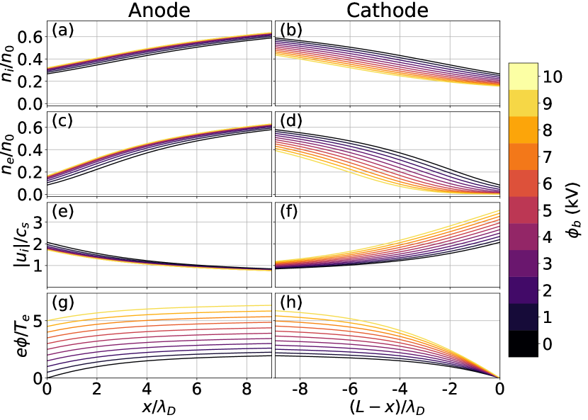
Figure 1: Normalized sheath profiles of the ion density (a,b), electron density (c,d), ion drift velocity (e,f), and electric potential (g,h) near the anode and the cathode are found by solving Eqs. 20-22 for bias potentials of 0 to 10 $\mathrm{kV}$. These profiles are used as the initial conditions for the simulations. See Appendix A for more information on how these profiles are calculated.

Eqs. 9 and 10 are solved using the code Gkeyll.[33, 34, 35] They are discretized using the discontinuous Galerkin method with an orthonormal modal serendipity basis with a polynomial order of 2. Eq. 9 is integrated in time using a 3-stage $3^{\text{rd}}$-order strong stability preserving Runge-Kutta method.[36] Eq. 10 is solved using a direct matrix inversion.

The Dirichlet boundary conditions for the Poisson equation are defined such that the electric potential at the anode and cathode are $\phi_{b}$ and 0, respectively. 1X-1V simulations are performed with bias potentials ranging from 0 to $10\text{\,}\mathrm{kV}$ in increments of $1\text{\,}\mathrm{kV}$ based on observations from FuZE.[19]

In addition, one 1X-2V simulation is performed for $5\text{\,}\mathrm{kV}$ to obtain an understanding of how the additional velocity dimension impacts the solution.

V Results and Discussion

All of the results in this section are taken from simulations that have reached a quasi-steady state at $t=20000\omega_{pe}$ where $\omega_{pe}=\sqrt{n_{0}e^{2}/m_{e}\epsilon_{0}}$ is the plasma frequency.

V.1 1X-1V Results

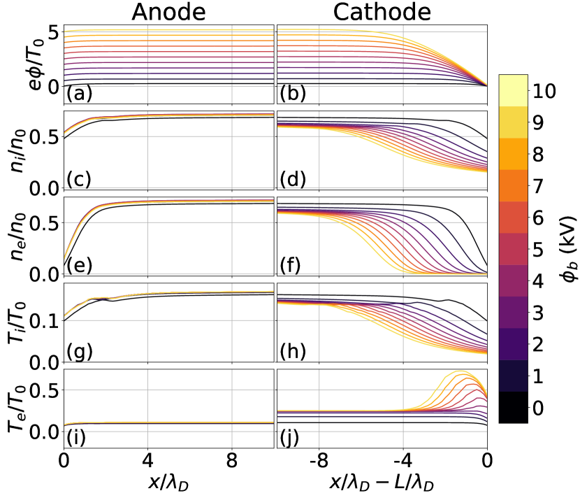
Figure 2: Plots of the normalized electric potential (a,b), ion density (c,d), electron density (e,f), ion temperature (g,h), and electron temperature (i,j) profiles near the anode and cathode for bias potentials from 0 to $10\text{\,}\mathrm{kV}$.

Fig. 2 shows the profiles of the normalized electric potential, ion density, electron density, ion temperature, and electron temperature in the region of $10\lambda_{D}$ near the anode and cathode for varying bias potentials.

The electric potential near the anode, Fig. 2(a), retains the same general shape and visually appears to translate upward with increasing bias potential. In other words, the potential drop at the anode does not change significantly with bias potential. Therefore, the ion density, electron density, ion temperature, and electron temperature at the anode minimally change with bias potential, as shown in Figs. 2(c,e,g,i), respectively.

In contrast, the electric potential drop near the cathode gets larger with increasing bias potential, as seen in Fig. 2(b), resulting in substantially different profiles for the other variables. The ion and electron density profiles, Figs. 2(d,f), respectively, show a reduction in density with increasing bias potential. In addition, the point at which the densities begin to decrease substantially moves further away from cathode (to the left) with increasing bias potential. In other words, as will be shown later in Fig. 6(l), the sheath length increases with bias potential. The potential barrier is large enough to drive the electron density to 0 at large bias potentials. Furthermore, the region in which the electrons have a near zero density becomes larger with increasing bias potential. The ion temperature, Fig. 2(h) shows a similar trend to the ion density. The electron temperature, Fig. 2(j), however, behaves differently. In general, the electron temperature near the cathode increases with bias potential. However, for bias potentials starting at around $4\text{\,}\mathrm{kV}$, a local maximum develops near the cathode. As the bias potential continues to increase, this local maximum gets larger and shifts further away from the cathode (to the left). This is partly due to the electron density tending to zero at higher bias potentials; note how the density is in the denominator in Eq. 17.

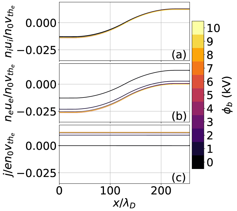
Figure 3: Plots of the normalized ion particle flux (a), electron particle flux (b), and current density (c) for varying bias potentials. The ion particle flux changes minimally with bias potential. The electron particle flux and current density reach an asymptotic limit as bias potential increases.

Unlike a classical sheath where there is expected to be no current within the plasma, the inclusion of a bias potential causes a current to develop across the entire domain. Fig. 3 shows the normalized ion particle flux, electron particle flux, and current density. All of these quantities use the electron thermal velocity as one of their normalization factors to make fair comparisons. The ion particle flux, Fig. 3(a), does not change with bias potential retaining its antisymmetry about the center of the domain. Therefore, the ion drift velocity in the sheath near the cathode increases with bias potential because the ion density near the cathode decreases, as shown in Fig. 2(d). The electron particle flux, Fig. 3(b), stays the same shape, but is translated in the negative direction as bias potential increases. The result is that the current density is constant in space for all bias potentials, as shown in Fig. 3(c). Furthermore, as the bias potential increases the electron particle flux, and therefore the current density, converge to asymptotic profiles. Figs. 3(a,b) show that, at high bias potentials, the current is entirely ion driven near the cathode, whereas it is predominantly electron driven toward the anode.

In addition, the electron particle flux tends to 0 near the cathode. This is a direct result of the chosen boundary condition: the perfectly absorbing wall. By definition, any electron particle flux that flows into the cathode (positive $x$ direction) must leave the domain. Therefore, directly at the cathode, the minimum possible value of the electron particle flux is 0. Thus, with increasing bias potential, the current density must saturate to the value of the ion particle flux at the cathode, as is shown theoretically in Eq. 8. The current density saturation and how it compared to theory from Eq. 8 is examined more closely in the discussion around Fig. 5. Future work will examine what impact wall emissions may have on the current density and the sheath dynamics.[26, 27]

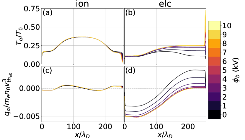
Figure 4: Plots of the normalized temperature (a,b) and heat flux (c,d) of the ions (a,c) and electrons (b,d) for varying bias potentials. The 0 value for the heat fluxes is highlighted with a dashed black line. The ion properties do not change much with bias potential whereas the electron properties change substantially.

Fig. 4 shows that the electrons, unlike the ions, change significantly with bias potential. Near the anode and in the center of the domain, the ions remain generally unaffected by the bias potential due to their significantly larger mass than the electrons. Near the cathode, however, the ion temperature and heat flux decrease with bias potential.

The electron temperature, Fig. 4(b), toward the anode is minimally affected by bias potential. However, this is not the case in the center of the domain and much less toward the cathode where the electron temperature increases with increasing bias potential. Except for near the cathode, the electron temperature profile reaches an asymptotic limit by about $3\text{\,}\mathrm{kV}$. Near the cathode, the local maximum that develops continues to increase with increasing bias potential, as also shown in Fig. 2(j).

The electron heat flux, Fig. 4(d), becomes more negative with increasing bias potential. This matches the trend seen in the electron particle flux, as shown in Fig. 3(b). As expected, for the zero bias potential case, the electron heat flux is antisymmetric about the center. However, as the bias potential increases, the location where the heat flux is zero (dashed black line) moves towards the cathode indicating that higher potential increases electron heat flux at the anode. Eventually, the electron heat flux reaches an asymptotic profile with the heat flux becoming significant at the anode and negligible at the cathode at larger bias potentials. The saturation of the electron heat flux is what causes the saturation of the electron temperature. The spikes in electron temperature near the cathode are attributed to a significantly decreasing density and a non-Maxwellian distribution.

It is important to note how the temperatures, Figs. 4(a-b), are significantly lower than what was initialized ($T_{0}=$2\text{\,}\mathrm{keV}$$). Lower temperatures are expected in simuations of sheaths in the absence of a high temperature source that does not replenish the energy that is lost to decompressional cooling. The impact of a high temperature source will be explored in subsequent work. Furthermore, the simulation results shown thus far are in only one velocity dimension. This inherently assumes that the plasma temperature is isotropic, which is not the case for a plasma sheath.[25] The inclusion of more velocity dimensions, as discussed in Sec. V.2, allows for better thermalization through collisions with the hotter perpendicular temperature.

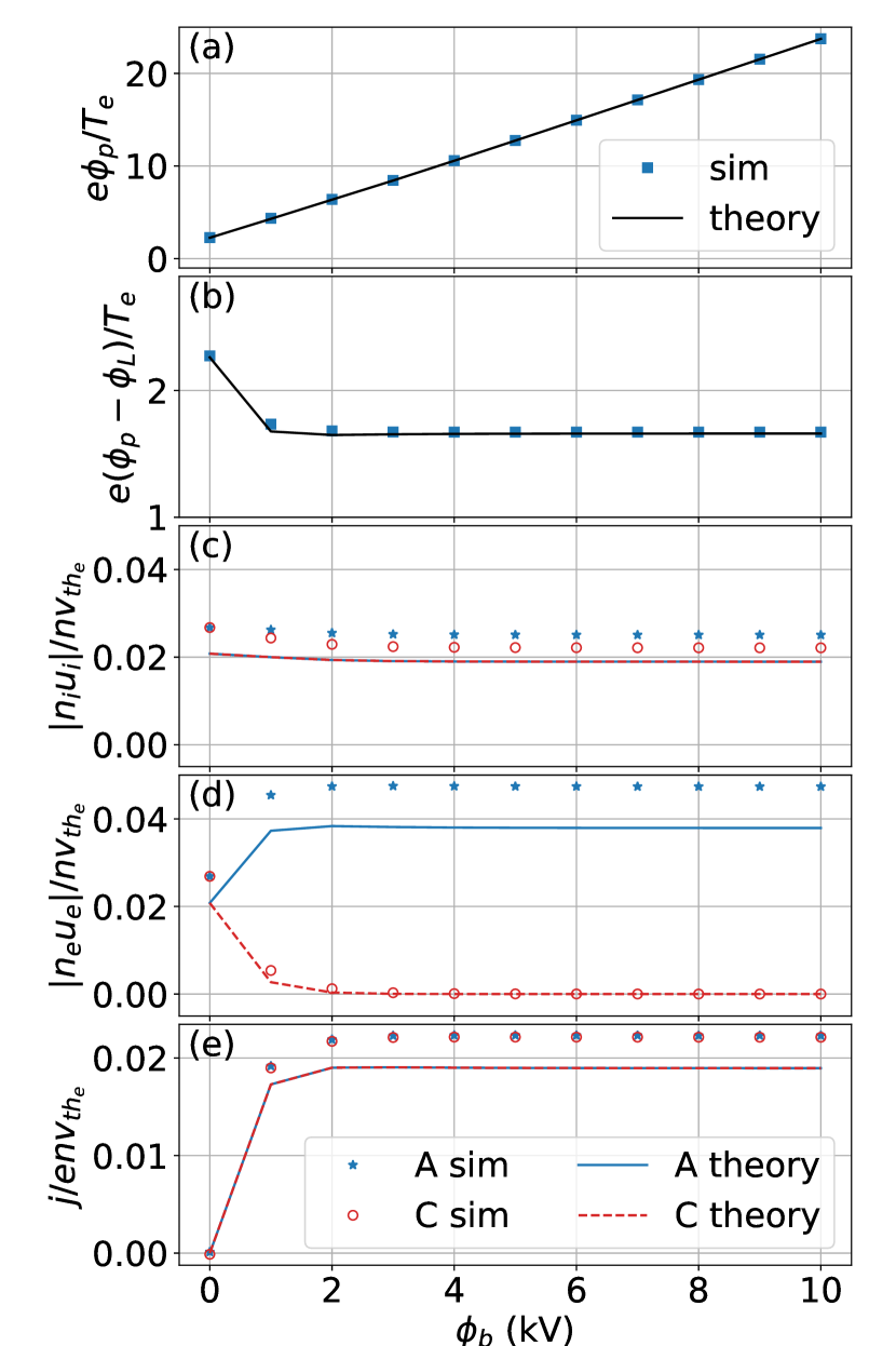
Figure 5: A comparison of the simulaton results to theory[1] on the effect of bias potential. Panel (a) shows the normalized plasma potential, defined as the potential at the center of the domain. Panel (b) shows the normalized difference between the plasma potential and the potential at the anode. For Panels (a-b), the squares represent the simulation values whereas the solid black line represents the theory. Panels (c-e) show the normalized ion particle flux, electron particle flux, and current density, respectively, at the anode (A) and cathode (C). The blue stars and red circles correspond to the simulation results at the anode and cathode, respectively. The blue solid line and the red dashed line correspond to the theory at the anode and cathode, respectively. Note that Panels (c-d) show absolute values to more easily convey the data; the particle fluxes at the anode are negative (going into the wall). Unlike the other plots, all normalizations in this plot use the values at the center of the domain.

Fig. 5 shows how well certain values from simulation compare with the theory from Sec. II. The theory, denoted by the lines, is calculated using the densities and temperatures at the center of the domain. The axis normalizations also use the center values.

Fig. 5(a) shows the comparison of the plasma potential, defined as the electric potential in the center of the domain, between simulation (blue squares) and theory (solid black line) based on Eq. 2. The simulation is well predicted by the theory. Since the ground potential is defined to be at the cathode, the plasma potential is equivalent to the potential drop between the center of the domain and cathode. Fig. 5(b) shows how the potential drop at the anode changes with bias potential. In corroboration with Fig. 2(a), the potential difference at the anode remains relatively constant with bias potential. The simulation results are compared to the theoretical difference, which is calculated as $\tilde{\phi}_{p}-\tilde{\phi}_{b}$, or the difference between Eq. 2 and $\tilde{\phi}_{b}$. Again, the simulation results agree well with theory.

Fig. 5(c) compares the ion particle flux at the electrodes with theory, Eqs. 3 and 5, respectively. The flux at the anode changes slightly with bias potential, whereas the flux at the cathode remains constant; both are higher than predicted by theory. Fig. 5(d) compares the electron particle flux at the anode and cathode with theory, Eqs. 4 and 6, respectively. The electrons follow the general trend of the theory, but saturate to a higher value than predicted. The electron particle flux at the cathode decreases with bias potential and asymptotes to 0, matching theory. Fig. 5(e) compares the current density at the electrodes with theory, Eq. 7. As also shown in Fig. 3(c), the current density at the electrodes are the same, with the points lying on top of each other. For the classical sheath case, the theoretical result is exactly met with there being no current in the plasma. For every other case, the current density is larger than predicted by theory.

The potential differences match well with theory. However, there are differences between theory and simulation for the particle fluxes, and therefore the current density. The theory assumes an isothermal fluid plasma with Boltzmann distributed electrons.[1] As shown in Figs. 2(g-j) and 4(a-b), the temperature is not isothermal. Therefore the Bohm speed used in Eq. 3 and 5 is expected to have $\gamma_{e}=\gamma_{i}=3$ (for a 1D plasma) instead of 1, which would increase the current.[22] Furthermore, the simulation model is fully kinetic and evolves the entire distribution function. Thus, there are additional kinetic physics that are not captured within the theory, such as the impact of heat flux. Therefore, the simplified theory underpredicts the actual particle fluxes and current density.

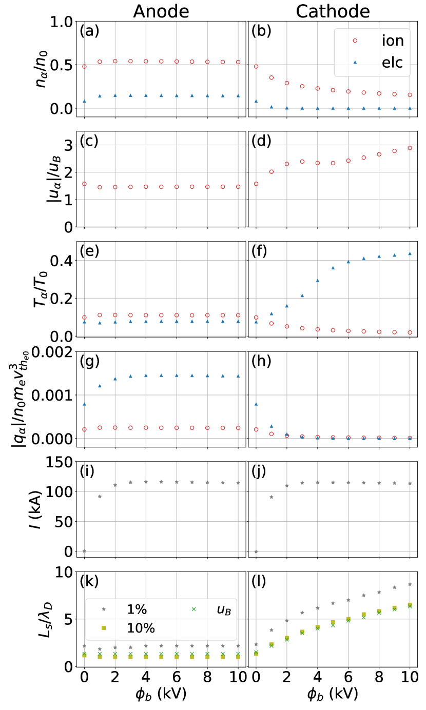
Figure 6: Plots of normalized densities (a,b), particle fluxes (c,d), temperatures (e,f), heat fluxes (g,h), current (i,j), and sheath lengths (k,l) at the electrodes as functions of the bias potential. Note that the absolute value of the particle and heat fluxes are plotted; at the anode, these are negatively valued. The red circles and blue triangles correspond to the ions and electrons, respectively. All values except for the current, Panels (i-j), are normalized. Note that the drift velocity, Panels (c-d) are normalized by the local Bohm speed.

Fig. 6 shows the values of the normalized density, ion drift velocity, temperature, heat flux, current, and sheath length at the electrodes as functions of the bias potential. These are reported to provide insight into the conditions the electrodes face which can inform future design choices. In line with the findings of the anode profiles in Fig. 2, the density, drift velocity, and temperature for the ions and electrons, Figs. 6(a,c,e), change minimally with bias potential. While the ion heat flux negligibly changes with bias potential, the electron heat flux slightly increases with bias potential, reaching an asymptotic value, as shown in Fig. 6(g).

The story is different at the cathode for Figs. 6(b,d,f,h). The ion density and temperature both decrease with increasing bias potential. The ion drift velocity increases significantly with bias potential, which should be expected based on ion particle flux remaining constant but the ion density decreasing. The ion heat flux tends to zero at the cathode. The electron properties at the cathode show much larger changes. The electron density and heat flux tend to zero at the cathode with increasing bias potential. The electron temperature at the cathode, however, increases with bias potential; it increases quickly at first, but then the rate slows down suggesting the possibility of an asymptotic limit at even higher bias potentials. Both the ion and electron heat fluxes decrease significantly with bias potential with both of them approaching 0 by approximately $3\text{\,}\mathrm{kV}$.

Thus, based on Figs. 5(c-d) and 6(g-h), the particle and heat fluxes that the anode and cathode face are different. For high bias potentials, both electrodes face the same ion particle flux. However, the anode faces approximately twice hte amount of electron particle flux while the cathod faces almost no electron particle flux. Additionally, at the anode, the ion heat flux remains approximately constant with bias potential while the electron heat flux increases significantly. However, the ion and electron heat fluxes both tend to zero at the cathode for high bias potentials. Therefore, the material choice for the anode needs to account for larger particle and heat fluxes, whereas this is less of a design concern for the cathode.

Figs. 6(i-j) show the current in $\mathrm{kA}$ at the anode and cathode, respectively. The current is calculated assuming it is perfectly uniform across a cylindrical Z-pinch. In other words, the current is $I=j\pi a^{2}$, where $a$ is the pinch radius. For the FuZE parameter regime,[16] the pinch radius is $3\text{\,}\mathrm{mm}$. As expected from Fig. 3(c), the currents at both electrodes are identical. FuZE reports a current of about $200\text{\,}\mathrm{kA}$,[16] whereas the simulation current asymptotes to about $115\text{\,}\mathrm{kA}$. The differences are largely explained by the lower temperature in the domain and assumptions made for the radial current profile. A similar calculation based purely on the simplified theory of Eq. 8 using the initial parameters yields a current of $154\text{\,}\mathrm{kA}$. If instead we use the simulation density and temperature at the center of the domain, we obtain a current of $97\text{\,}\mathrm{kA}$, which is lower than the simulation current as is also shown in Fig. 5(e); the theory underpredicts the current that develops. Therefore, it is anticipated that in a case with less decompressional cooling in the domain such that the steady state temperature is closer to the initialized temperature, the current output will be higher than the predicted $154\text{\,}\mathrm{kA}$.

Figs. 6(k-l) show how the sheath lengths change with bias potential. The sheath lengths are calculated in three ways: 1% fractional charge density, 10% fractional charge density, and Bohm speed. The fractional charge density is defined as $|n_{i}-n_{e}|/(n_{i}+n_{e})$. While more sophisticated theory has been developed for the Bohm speed accounting for transport and anisotropies,[22, 23] a simplified Bohm speed is used here: $u_{B}=\sqrt{\gamma(T_{i}+T_{e})/m_{i}}$, where $\gamma$ is the ratio of specific heats. For one velocity dimension (or degree of freedom), $\gamma$ is 3. The sheath length is determined based on the location where the ratio of the ion velocity to the Bohm speed, $u_{i}/u_{B}$, is 1 or where the the fractional charge density is either 1% or 10%. The results for the anode show that the sheath length does not change significantly with bias potential. For the cathode, the sheath length increases with bias potential as expected based on Figs. 2(d,f). This is because the electrons, being much less massive, are impacted more heavily by the larger bias potentials creating a larger region of positive charge.

V.2 Comparison with 1X-2V

Due to the large computational expense, one 1X-2V simulation is performed with a $5\text{\,}\mathrm{kV}$ bias potential to understand how the additional velocity dimension impacts the solution. The results presented here are at $t=20000\omega_{pe}$, by which point the plasma has reached a quasi-steady state.

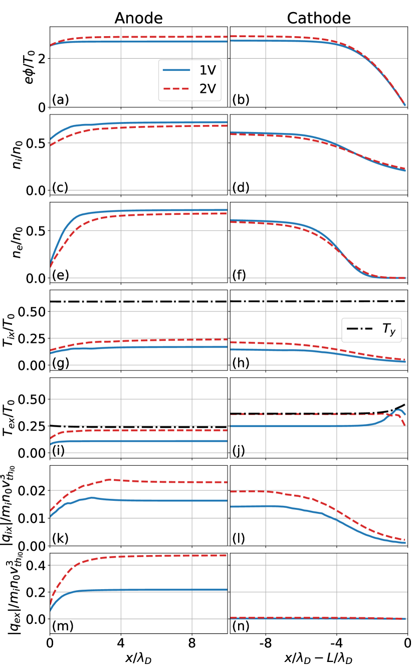
Figure 7: Comparison of normalized sheath profiles for the electric potential (a,b), densities (c-f), temperatures (g-j), and heat fluxes (k-n) between a 1X-1V (solid blue line) and 1X-2V (dashed red line) simulation for $\phi_{b}=$5\text{\,}\mathrm{kV}$$. The black dash-dot line in Panels (e-h) represents the $y$, or perpendicular, direction temperature from the 1X-2V simulations. In general, the differences between the profiles near the cathode are minimal, whereas they are more substantial at the anode.

Fig. 7 shows a comparison of the 1X-1V results to the 1X-2V results for sheath profiles near the electrodes of the electric potential, densities, temperatures, and heat fluxes. This plot is directly analagous to Fig. 2. Figs. 7(a-b) show the electric potential near the electrodes. For about 1 Debye length near the anode and about 4 Debye lengths near the cathode, the electric potential for the 1X-1V and 1X-2V cases are approximately the same. However, the electric potential towards the center of the domain, or the plasma potential, of the 1X-2V case is larger than that of the 1X-1V case. Therefore, the potential drop is larger at both electrodes, which results in sharper sheath phenomena. Relatively, the difference in the potential drop is larger at the anode than at the cathode. In other words, the potential difference between the center of the domain and cathode is already large for the 1X-1V case and only increases in the 1X-2V case by 9.4%. The potential difference between the center of the domain and the anode is comparatively small for the 1X-1V case and increases in the 1X-2V case by 71.9%. Therefore, the anode sheath is affected more prominently than the cathode sheath.

Following the pattern of the electric potential, the ion and electron density near the cathode, Figs. 7(d,f), only show a minimal decrease while the densities near the anode, Figs. 7(c,e), show a more notable decrease.

The temperatures in the domain are generally larger, as seen in Figs. 7(g-j). In addition, due to considering kinetic physics, the particle distribution, unlike in the fluid approximation, is not required to be isotropically Maxwellian. Therefore, temperature, as defined by Eq. 17, can be different in each direction. Here, we define parallel ($x$) as in the direction of the flow. Therefore the $y$ direction is the perpendicular direction. In the parallel direction, there exists a heat sink with the perfectly absorbing wall boundary condition. In the perpendicular direction, however, there is no such heat sink. Therefore, an anisotropy develops in the temperature. The dash-dot black line depicts the temperature in the $y$ or perpendicular direction. Unlike the parallel temperature, the perpendicular temperature increases in the sheath; this increase is much larger at the cathode than at the anode. This is due to the gradient of the parallel heat flux of the perpendicular degrees of freedom.[37]

The ion heat fluxes are larger in the 1X-2V simulation, as shown in Figs. 7(k-l). The electron heat flux, Figs. 7(m-n), is only larger near the anode; near the cathode, it remains close to zero as with the 1X-1V case.

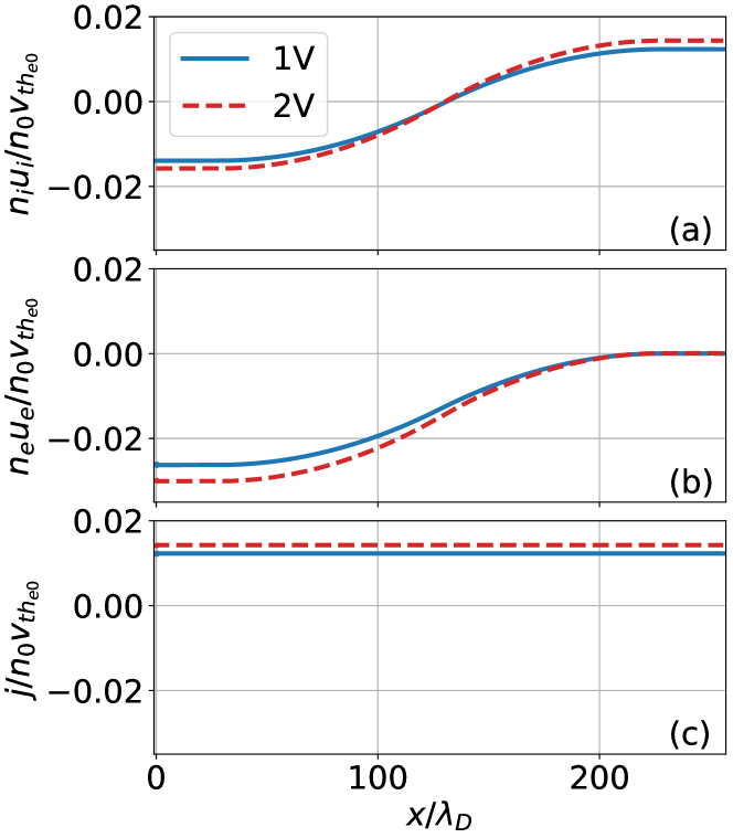
Figure 8: Comparisons of the normalized ion particle flux (a), electron particle flux (b), and current density (c) between a 1X-1V (solid blue line) and 1X-2V (dashed red line) simulation with $\phi_{b}=$5\text{\,}\mathrm{kV}$$.

Fig. 8 shows the comparison of the normalized particle flux and current between the 1X-1V and 1X-2V simulations. This figure is directly analogous to Fig. 3. The ion particle flux, Fig. 8(a), is 13.1% larger in magnitude in the 1X-2V case. This is due to the higher general temperature in the domain. The electron particle flux, Fig. 8(b), still goes to zero at the right wall, but is 14.4% larger in magnitude at the anode. The result is that the current density, Fig. 8(c), is 15.9% larger in the 1X-2V case. The current density is still spatially constant. If a similar calculation is done as that in Figs. 6(i-j) to obtain an estimated current assuming a perfectly uniform Z-pinch, we find that the 1X-2V case yields a current of $134\text{\,}\mathrm{kA}$.

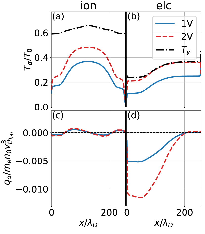
Figure 9: Comparisons of normalized temperature (a,b) and heat flux (c,d) for ions (a,c) and electrons (b,d) between the 1X-1V (solid blue line) and 1X-2V (dashed red line) simulations with $\phi_{b}=$5\text{\,}\mathrm{kV}$$. The black dash-dot line represents the temperature in the $y$ (perpendicular) direction.

Fig. 9 compares how the temperatures and heat fluxes vary between the 1X-1V and 1X-2V simulations. The inclusion of the second velocity dimension allows for an anisotropy to develop in the sheath region for the temperature. Note that there is still cooling in 1X-2V, but since decompressional cooling primarily impacts the parallel temperature, the presence of the perpendicular temperature with presheath collisions permits higher temperatures in the domain (compared to 1X-1V) late in time. This is the primary reason why the plasma potential and the ion particle flux are larger for the 1X-2V simulations. The electron temperature shows anisotropy only near the electrodes, with the parallel and perpendicular temperatures being the same in the center of the domain. However, an anisotropic equilibrium develops for the ion temperature due to the energy loss in the parallel direction being larger than that of the perpendicular direction and the collisional isotropization.

The ion heat flux does not change much with the inclusion of the second velocity dimension compared to how much the electron heat flux changes for the 1X-2V case. Near the cathode, the electron heat flux remains close to zero. However, it increases sharply towards the anode and has a much larger drop at the anode. This suggests that the 1X-1V simulations underpredicts the electron heat flux for the entire domain apart from near the cathode. Therefore, even more care needs to be taken in material choice at the anode due to the higher fluxes.

VI Summary and Conclusions

Continuum kinetic simulations of a proton-electron plasma are performed solving the Boltzmann-Poisson system to model the sheath formation of a plasma bounded between two walls, or electrodes, with an electric potential bias between them. The parameter regime is chosen to be relevant to Z-pinch fusion experiments.

1X-1V simulations are performed with bias potentials ranging from 0 to $10\text{\,}\mathrm{kV}$. The results suggest that the sheath formation at the left wall, or anode, does not change greatly with bias potential. The right wall, or cathode, however, exhibits a much steeper potential drop, resulting in greater differences in sheath formation. Near the cathode, the ion and electron densities, ion temperature, and ion and electron heat fluxes decrease with bias potential. The electron temperature, however, increases with bias potential.

The ion particle flux does not change significantly within the entire domain with varying bias potential. The electron particle flux becomes more negative with increasing bias potential, reaching an asymptotic limit when the particle flux at the cathode reaches zero. For all cases, the current density is spatially constant and increases with bias potential. Because the ion particle flux does not change and the electron particle flux reaches an asymptotic limit, the current density also reaches a limit with increasing bias potential. The current is predominantly carried by the electrons at the anode and by the ions at the cathode.

The 1X-1V simulations match well with theory for the plasma potential. The simulation trends well with the theory for the particle fluxes. However, the theory underpredicts the simulation results for current and fluxes. The differences are explained by additional kinetic physics and fewer assumptions considered in the simulations.

Particle and heat fluxes for the ions and electrons at both electrodes are provided. Assuming the current is carried uniformly in the Z-pinch with FuZE parameters, the current from the simulations asymptote to $115\text{\,}\mathrm{kA}$ with increasing bias potential, as compared to the $200\text{\,}\mathrm{kA}$ measured in FuZE.

At the anode, the ion particle and heat fluxes remain relatively constant with bias potential; the electron particle and heat fluxes increases by a factor of approximately 2 at high bias potentials. At the cathode, however, the electron particle flux, electron heat flux, and ion heat flux tend to zero at higher bias potentials, whereas the ion particle flux remains constant. Therefore for high bias potentials, the material choice for the anode needs to consider higher fluxes from the ions and electrons; for the cathode, only the ion particle flux needs to be considered.

A 1X-2V simulation is run for the $5\text{\,}\mathrm{kV}$ bias potential case. The results show a temperature anisotropy develop in the sheath region. In general, the sheath effects are more stark than those from the 1X-1V simulations. The increase is attributed to the second velocity dimension causing less overall cooling in the system due to collisions involving the perpendicular temperature. The increased overall temperature of the plasma also contributes to a 15.9% increase in the current. Simulations performed with higher velocity dimensions produce reduced cooling and larger currents, which are closer to the experimental values.

Future work will leverage recent developments that may permit computationally-efficient calculations using higher velocity dimensions. Additionally, the impact of physical wall materials on sheaths will be studied with biased potentials in subsequent work.

Data Availability Statement

Readers may reproduce our results and also use Gkeyll for their applications. The code and input files used here are available online. Full installation instructions for Gkeyll are provided on the Gkeyll website.[33] The code can be installed on Unix-like operating systems (including Mac OS and Windows using the Windows Subsystem for Linux) either by installing the pre-built binaries using the conda package manager (https://www.anaconda.com) or building the code via sources. The input files used here are under version control and can be obtained from the repository at https://github.com/ammarhakim/gkyl-paper-inp/tree/master/2022_PoP_BiasedWallSheaths.

Appendix A 1D Initial Sheath Approximation

The initial conditions used in the simulations (see Fig. 1) are calculated based on theory from Ref. 4. With some a priori predictions of the electric potential drop near the wall and the ion particle flux at the wall, theoretical profiles can be obtained of the ion density, electron density, ion velocity, and electric potential.

The system of ordinary differential equations (ODEs) that describe the steady state sheath behavior are[4]

$$\frac{d\tilde{\phi}}{d\tilde{x}} =-\tilde{E}$$ (20)

$$\frac{d\tilde{E}}{d\tilde{x}} =\frac{\tilde{R}\tilde{x}}{\tilde{u}_{i}}-\exp\tilde{\phi}$$ (21)

$$\frac{d\tilde{u}_{i}}{d\tilde{x}} =\frac{\tilde{E}}{\tilde{u}_{i}}-\frac{\tilde{u}_{i}}{\tilde{x}},$$ (22)

where $R$ is an ionization source term and the tildes denote normalized variables. These ODEs must be solved numerically. The Python package odeint is used for the numerical integration and uses a combination of the nonstiff Adams method and the stiff backwards difference method.[39]

Consider a domain that spans from 0 to $\tilde{L}=L/\lambda_{D}$ where $L$ is the domain length. At $\tilde{x}=0$, the normalized ion and electron densities are 1 and the normalized electric potential, electric field, and ion velocity are 0. The starting point for the integration, however, cannot be $\tilde{x}=0$ due to division by zero (see Eq. 22). Instead, the integration begins at $\tilde{x}=\Delta\tilde{x}$ where $\Delta\tilde{x}=\tilde{L}/N$ where $N$ is the number of points considered in the domain. Thus, the initial conditions for the electric potential, electric field, and velocity are $-\tilde{R}^{2}\Delta\tilde{x}^{2}$, $2\tilde{R}\Delta\tilde{x}$, and $\tilde{R}\Delta\tilde{x}$, respectively.[4]

Ref. 4 suggests integrating in $\tilde{x}$ until the potential drop at the wall reaches a pre-defined value. The a priori value can be calculated as the difference between the plasma potential, Eq. 2, and the potential at the wall. However, there is a second constraint at the wall that must also be met; based on the steady state continuity equation, the ion particle flux at the wall must be $\tilde{n}_{i}\tilde{u}_{i}|_{w}=\tilde{R}\tilde{L}$.[4] If we just solve the system of ODEs until the potential drop is reached, the ion particle flux constraint is not necessarily met. This issue is resolved by iterating on $\tilde{L}$ until both the potential and particle flux constraints are met.

The inputs of the developed algorithm are the potential drop and the ion particle flux at the wall. Note that this algorithm assumes that the plasma potential (the potential in the center of the domain) is the ground potential. Therefore, the input potential drop should be negative. Parts of this algorithm are adapted from a code in Sec. 5.1.3 of Ref. 32. An arbitrarily small $\tilde{L}$ is chosen as the initial domain length. Therefore, the ionization source term must be $\tilde{R}=\tilde{n}_{i}\tilde{u}_{i}|_{w}/\tilde{L}$. The ODEs are numerically integrated across the entire domain using odeint. Then the value at the wall is tested for the electric potential constraint; note that the ion particle flux constraint is automatically satisfied through the definition of $\tilde{R}$. The domain length is iterated on systematically to reach the correct solution. Additionally, define a switch, $r$, to note when the electric potential at the wall first becomes less than the input potential. Due to the assumed monotonicity of the potential profile, this is equivalent to the tested domain length being larger than the final converged domain length. Alg. A describes how we iteratively converge to the solution.

[!htb] Algorithm to solve Eqs. 20-22 iteratively by changing domain length

1:$\Delta\tilde{\phi}$ and $\tilde{n}_{i}\tilde{u}_{i}|_{w}$

2:Initial condition profiles for $\tilde{n}_{i}$, $\tilde{n}_{e}$, $\tilde{u}_{i}$, and $\tilde{\phi}$

3:Set initial arbitrarily small $\tilde{L}_{0}$

4:for $i\leftarrow 0$ to max_iter do

5:     Build $\tilde{x}$ grid

6:     $\tilde{R}\leftarrow\tilde{n}_{i}\tilde{u}_{i}|_{w}/\tilde{L}_{i}$

7:     Set ODE initial conditions

8:     Solve ODEs using odeint

9:     if $\Delta\tilde{\phi}-TOL\leq\tilde{\phi}_{w}\leq\Delta\tilde{\phi}+TOL$ then

10:         break

11:     else if $\tilde{\phi}_{w}>\Delta\tilde{\phi}$ and $r=0$ then

12:         $\tilde{L}_{i+1}\leftarrow 2\tilde{L}_{i}$

13:     else if $\tilde{\phi}_{w}>\Delta\tilde{\phi}$ and $r=1$ then

14:         $\tilde{L}_{i+1}\leftarrow\tilde{L}+\Delta\tilde{L}_{i}/2$

15:     else if $\tilde{\phi}_{w}<\Delta\tilde{\phi}$ then

16:         $r\leftarrow 1$

17:         $\tilde{L}_{i+1}\leftarrow\tilde{L}-\Delta\tilde{L}_{i}/2$

18:     end if

19:     $\Delta\tilde{L}\leftarrow|\tilde{L}_{i+1}-\tilde{L}_{i}|$

20:end for

There are two known failure modes for this algorithm. It is possible that the solution converges to some $\tilde{L}$ at which the electric potential is not within the tolerance ($TOL$) of the input potential. In this case, if $\Delta\tilde{L}$ is less than the tolerance, then the solution is assumed to have converged to the best possible solution. The other failure mechanism is that the solution can diverge and the electric potential constraint will never be satisfied; therefore, no solution can be found. These failure modes arise based on the inputs of the ion particle flux and electric potential at the wall. For ion particle fluxes that are too low (generally lower than 0.51), the solution diverges. Additionally, the electric potential at the wall must be negative.

The profiles in Fig. 1 are found by using Alg. A. The ion particle flux input is set as $\tilde{n}_{i}\tilde{u}_{i}|_{w}=0.55$. The potential input is set based on the definitions in Sec. II; the potential drops used for the anode and cathode are $\Delta\tilde{\phi}|_{A}=\tilde{\phi}_{b}-\tilde{\phi}_{p}$ and $\Delta\tilde{\phi}|_{C}=-\tilde{\phi}_{p}$, respectively. To calculate the plasma potential, additional inputs of the ion mass, ion temperature, and electron temperature are needed. For these cases, we use the proton mass and $T_{i}=T_{e}=$2\text{\,}\mathrm{keV}$$.

References

- Stangeby [2000] P. C. Stangeby, The plasma boundary of magnetic fusion devices, Vol. 224 (Institute of Physics Pub. Philadelphia, Pennsylvania, 2000).
- Lieberman and Lichtenberg [2005] M. A. Lieberman and A. J. Lichtenberg, Principles of plasma discharges and materials processing (John Wiley & Sons, 2005).
- Baalrud et al. [2020] S. D. Baalrud, B. Scheiner, B. T. Yee, M. M. Hopkins, and E. Barnat, “Interaction of biased electrodes and plasmas: sheaths, double layers, and fireballs,” Plasma Sources Science and Technology 29, 053001 (2020).
- Robertson [2013] S. Robertson, “Sheaths in laboratory and space plasmas,” Plasma Physics and Controlled Fusion 55, 093001 (2013).
- Wollenhaupt, Le, and Herdrich [2018] B. Wollenhaupt, Q. H. Le, and G. Herdrich, “Overview of thermal arcjet thruster development,” Aircraft Engineering and Aerospace Technology (2018).
- Giuliani and Commisso [2015] J. L. Giuliani and R. J. Commisso, “A review of the gas-puff -pinch as an x-ray and neutron source,” IEEE Transactions on Plasma Science 43, 2385–2453 (2015).
- Weynants and Van Oost [1993] R. Weynants and G. Van Oost, “Edge biasing in tokamaks,” Plasma physics and controlled fusion 35, B177 (1993).
- Shumlak [2020] U. Shumlak, “Z-pinch fusion,” Journal of Applied Physics 127, 200901 (2020).
- Hartman et al. [1977] C. Hartman, G. Carlson, M. Hoffman, R. Werner, and D. Cheng, “A conceptual fusion reactor based on the high-plasma-density z-pinch,” Nuclear Fusion 17, 909 (1977).
- Bennett [1934] W. H. Bennett, “Magnetically self-focussing streams,” Physical Review 45, 890 (1934).
- Haines et al. [2000] M. Haines, S. Lebedev, J. Chittenden, F. Beg, S. Bland, and A. Dangor, “The past, present, and future of z pinches,” Physics of Plasmas 7, 1672–1680 (2000).
- Shumlak et al. [2001] U. Shumlak, R. Golingo, B. Nelson, and D. Den Hartog, “Evidence of stabilization in the z-pinch,” Physical review letters 87, 205005 (2001).
- Shumlak et al. [2003] U. Shumlak, B. Nelson, R. Golingo, S. Jackson, E. Crawford, and D. Den Hartog, “Sheared flow stabilization experiments in the zap flow z pinch,” Physics of Plasmas 10, 1683–1690 (2003).
- Shumlak et al. [2009] U. Shumlak, C. Adams, J. Blakely, B.-J. Chan, R. Golingo, S. Knecht, B. Nelson, R. Oberto, M. Sybouts, and G. Vogman, “Equilibrium, flow shear and stability measurements in the z-pinch,” Nuclear Fusion 49, 075039 (2009).
- Shumlak et al. [2017] U. Shumlak, B. Nelson, E. Claveau, E. Forbes, R. Golingo, M. Hughes, R. Oberto, M. Ross, and T. Weber, “Increasing plasma parameters using sheared flow stabilization of a z-pinch,” Physics of Plasmas 24, 055702 (2017).
- Zhang et al. [2019] Y. Zhang, U. Shumlak, B. Nelson, R. Golingo, T. Weber, A. Stepanov, E. Claveau, E. Forbes, Z. Draper, J. Mitrani, et al., “Sustained neutron production from a sheared-flow stabilized z pinch,” Physical review letters 122, 135001 (2019).
- Mitrani et al. [2019] J. M. Mitrani, D. P. Higginson, Z. T. Draper, J. Morrell, L. A. Bernstein, E. L. Claveau, C. M. Cooper, E. G. Forbes, R. P. Golingo, B. A. Nelson, et al., “Measurements of temporally-and spatially-resolved neutron production in a sheared-flow stabilized z-pinch,” Nuclear Instruments and Methods in Physics Research Section A: Accelerators, Spectrometers, Detectors and Associated Equipment 947, 162764 (2019).
- Claveau et al. [2020] E. Claveau, U. Shumlak, B. Nelson, E. Forbes, A. Stepanov, T. Weber, Y. Zhang, and H. McLean, “Plasma exhaust in a sheared-flow-stabilized z pinch,” Physics of Plasmas 27, 092510 (2020).
- Stepanov et al. [2020] A. Stepanov, U. Shumlak, H. McLean, B. Nelson, E. Claveau, E. Forbes, T. Weber, and Y. Zhang, “Flow z-pinch plasma production on the fuze experiment,” Physics of Plasmas 27, 112503 (2020).
- Shumlak et al. [2012] U. Shumlak, J. Chadney, R. Golingo, D. Den Hartog, M. Hughes, S. Knecht, W. Lowrie, V. Lukin, B. Nelson, R. Oberto, et al., “The sheared-flow stabilized z-pinch,” Fusion Science and Technology 61, 119–124 (2012).
- Scheiner et al. [2016] B. Scheiner, S. D. Baalrud, M. M. Hopkins, B. T. Yee, and E. V. Barnat, “Particle-in-cell study of the ion-to-electron sheath transition,” Physics of Plasmas 23, 083510 (2016).
- Li et al. [2022a] Y. Li, B. Srinivasan, Y. Zhang, and X.-Z. Tang, “Bohm criterion of plasma sheaths away from asymptotic limits,” Physical Review Letters 128, 085002 (2022a).
- Li et al. [2022b] Y. Li, B. Srinivasan, Y. Zhang, and X.-Z. Tang, “Transport physics dependence of bohm speed in presheath–sheath transition,” Physics of Plasmas 29, 113509 (2022b).
- Shumlak et al. [2011] U. Shumlak, R. Lilly, N. Reddell, E. Sousa, and B. Srinivasan, “Advanced physics calculations using a multi-fluid plasma model,” Computer Physics Communications 182, 1767–1770 (2011).
- Cagas et al. [2017] P. Cagas, A. Hakim, J. Juno, and B. Srinivasan, “Continuum kinetic and multi-fluid simulations of classical sheaths,” Physics of Plasmas 24, 022118 (2017).
- Cagas, Hakim, and Srinivasan [2020] P. Cagas, A. Hakim, and B. Srinivasan, “Plasma-material boundary conditions for discontinuous galerkin continuum-kinetic simulations, with a focus on secondary electron emission,” Journal of Computational Physics 406, 109215 (2020).
- Bradshaw et al. [2022] K. Bradshaw, P. Cagas, A. Hakim, and B. Srinivasan, “Plasma sheath studies using a physical treatment of electron emission from a dielectric wall,” (2022).
- Dougherty [1964] J. Dougherty, “Model fokker-planck equation for a plasma and its solution,” The Physics of Fluids 7, 1788–1799 (1964).
- Francisquez et al. [2020] M. Francisquez, T. N. Bernard, N. R. Mandell, G. W. Hammett, and A. Hakim, “Conservative discontinuous galerkin scheme of a gyro-averaged dougherty collision operator,” Nuclear Fusion 60, 096021 (2020).
- Hakim et al. [2020] A. Hakim, M. Francisquez, J. Juno, and G. W. Hammett, “Conservative discontinuous galerkin schemes for nonlinear dougherty–fokker–planck collision operators,” Journal of Plasma Physics 86 (2020).
- Wang et al. [2015] L. Wang, A. H. Hakim, A. Bhattacharjee, and K. Germaschewski, “Comparison of multi-fluid moment models with particle-in-cell simulations of collisionless magnetic reconnection,” Physics of Plasmas 22, 012108 (2015).
- Cagas [2018] P. Cagas, Continuum Kinetic Simulations of Plasma Sheaths and Instabilities, Ph.D. thesis, Virginia Polytechnic Institute and State University (2018).
- Gkeyll [2022] Gkeyll, (2022), https://gkeyll.readthedocs.io.
- Juno et al. [2018] J. Juno, A. Hakim, J. TenBarge, E. Shi, and W. Dorland, “Discontinuous galerkin algorithms for fully kinetic plasmas,” Journal of Computational Physics 353, 110–147 (2018).
- Hakim and Juno [2020] A. Hakim and J. Juno, “Alias-free, matrix-free, and quadrature-free discontinuous galerkin algorithms for (plasma) kinetic equations,” in SC20: International Conference for High Performance Computing, Networking, Storage and Analysis (IEEE, 2020) pp. 1–15.
- Gottlieb [2005] S. Gottlieb, “On high order strong stability preserving runge-kutta and multi step time discretizations,” Journal of scientific computing 25, 105–128 (2005).
- Zhang et al. [2022] Y. Zhang, Y. Li, B. Srinivasan, and X.-Z. Tang, “Resolving the mystery of electron perpendicular temperature spike in the plasma sheath,” arXiv preprint arXiv:2210.16711 (2022).
- Note [1] Https://docs.scipy.org/doc/scipy/reference/generated/scipy.integrate.odeint.html.
- Petzold [1983] L. Petzold, “Automatic selection of methods for solving stiff and nonstiff systems of ordinary differential equations,” SIAM journal on scientific and statistical computing 4, 136–148 (1983).