A complete spectroscopic catalogue of local galaxies in the Northern spring sky - Gas properties and nuclear activity in different environments

With the aim of providing the complete demography of galaxies in the local Universe, including their nuclear properties, we present SPRING, a complete census of local galaxies limited to the spring quarter of the Northern sky ($10\mathrm{h}<\mathrm{RA}<16\mathrm{h}$; $0^{\circ}<\mathrm{Dec}<65^{\circ}$). The SPRING catalogue is a flux- and volume-limited sample ($r<17.7$ mag, $cz<10000\ \mathrm{km\ s}^{-1}$) of 30597 galaxies, including the Virgo, Coma and A1367 clusters. Images and spectra were individually examined to clear the sample from unwanted entries.
To inspect possible secular and environmental dependencies of the various nuclear excitation properties (SF vs. AGN), we perform a multidimensional analysis by dividing the total sample according to (i) their position in the $(\mathrm{NUV}-i)$ vs. $M_{\rm star}$ diagram, (ii) local galaxy density, (iii) stellar-mass, (iv) halo-mass of the group to which galaxies belong, and (v) neutral Hydrogen content. We present a new calibration of the optical diameter-based H I-deficiency parameter $\mathrm{H}\thinspace\scriptsize{\text{I}}_{\mathrm{def}}$ employing a reference sample of isolated galaxies extracted from SPRING. At intermediate distances between Virgo and Coma, we identify a ring-like structure of galaxies constituted by three large filaments, each with approximately 20$h^{-1}$ Mpc length, mostly composed of blue-cloud galaxies with stellar-mass $M_{\rm star}\lesssim 10^{10}$ M_⊙. The fraction of H I-deficient galaxies within the filament ($\sim$30%) suggests that filaments are a transitioning environment between field and cluster in terms of H I content, as we find a clear progression from field galaxies to filament and cluster galaxies for increasing $\mathrm{H}\thinspace\scriptsize{\text{I}}_{\mathrm{def}}$ parameter.
We classify the nuclear spectra according to the four-line BPT and the two-line WHAN diagnostic diagrams, and investigate the variation in the fraction of active nuclei hosts with stellar-mass, as well as their colours and environments. We observe that the fraction of LINERs is a steep function of stellar-mass, e.g., it is consistent with zero up to $M_{\rm star}\lesssim 10^{9.5}$ M_⊙ and becomes $\sim$ 40 % for $M_{\rm star}\gtrsim 10^{10.5}$ M_⊙, whereas, for $M_{\rm star}\lesssim 10^{9-9.5}$ M_⊙, almost the entire spectroscopic sample is constituted of galaxies with star-forming nuclei. We investigate whether the nuclear-excitation fractions depend predominantly on the stellar-mass or, conversely, on the galaxy environment. In general, we observe that the mass-dependency of the fraction of Seyfert nuclei is little sensitive to the galaxy environment, whereas the fraction of star-forming nuclei is a steeper function of stellar-mass in lower-density environments and in blue-cloud galaxies. We find that the fraction of LINERs depends on galaxy colour and, for $M_{\rm star}\gtrsim 10^{9.5-10}$ M_⊙, increases in galaxies belonging to the green valley.

1 Introduction

The spring sky, comprised between 10 and 16 hours of right ascension in the Northern hemisphere, has hosted most of the near-field cosmology studies in the history of astrophysics, due to several unique characteristics. It contains (i) the Northern Galactic Pole, the area less crowded by the Milky Way, which is thus less susceptible to dust extinction; (ii) the Local Supercluster, including (iii) the Virgo cluster, and (iv) the Coma cluster (with the “Great Wall”).

Starting from the 1950s, when the Palomar sky survey became available, a large number of astronomers interested in near-scale cosmology (e.g., Fritz Zwicky, Allan Sandage, Gerard de Vaucouleurs, and collaborators) focused their work in this region of the sky using photographic material taken at 1.5-2.5 meter-class telescopes (see, e.g., Zwicky et al. 1961; Tully 1982; Einasto et al. 1983; Binggeli et al. 1985). Their goal was to shed light onto the physical mechanisms that govern the structure of the Universe on local scale (within the distance of the Coma cluster, i.e., $\sim$100$h^{-1}$ Mpc). Among the early studies, many efforts aimed to establish the scale relations that govern the evolution of galaxies, such as, for example, the “downsizing” law Gavazzi et al. (1996).

At the turn of the millennium, the digital revolution took place with the announcement of the Sloan Digital Sky Survey (SDSS, York et al. 2000). The SDSS combined five-band ($u,g,r,i,z$) photometry from digital imaging with exquisite medium resolution ($R\approx 2000$) spectroscopy taken (except for few cases) in the nuclei of external galaxies brighter than $17.7$ mag in the $r$-band. However, instead of reforming the study of the Local Supercluster, the SDSS shifted the focus of near-field cosmology to a slightly higher redshift ($0.1\lesssim z\lesssim 0.5$). This turn was owing to the difficulty of extracting precise photometric parameters from digital images in areas crowded with extended galaxies using automatic algorithms because of significant overestimate of the sky background; another consequence of this effect is the so-called “shredding” that affects the SDSS photometry and spectroscopy of nearby galaxies Blanton et al. (2005a, b, c).

Because of these difficulties, the vast majority of near-field-cosmology works based on the SDSS are at $0.1\lesssim z\lesssim 0.5$ (see, e.g., Kauffmann et al. 2003b; Gómez et al. 2003; Blanton et al. 2017; Peng et al. 2010). Alternatively, a number of studies employed versions of the SDSS with improved background determination in case of very extended galaxies (e.g., the NASA-Sloan Atlas catalogue of Blanton et al. 2011), or with the limitation $z>0.01$ (which, anyway, excludes the Local Supercluster and the Virgo cluster). This is, for example, the case of Yang et al. (2007, 2008, 2009), who, despite limiting their sample (in this case, the DR4) to $0.01<z<0.2$, retain more than 360.000 galaxies in it. This number is sufficiently large to ensure a satisfactory statistical coverage of the sky, but is too large to allow the firsthand inspection of all galaxies (images and spectra) in search for errors (e.g., false objects caused by diffraction spikes of bright stars, duplicates, spectroscopy not taken at the centre of galaxies). Such mistakes do not affect the sample statistically, but pollute the catalogue with unwanted individual objects.

Besides the SDSS, another outcome of the third millennium digital revolution was the availability of multi-wavelength photometry (from the ultraviolet to the far-infrared bands) based on space missions such as GALEX Martin et al. (2005); Morrissey et al. (2007) and WISE Wright et al. (2010). Multi-wavelength data have proven to be very effective in the investigation of the role of the environment in galaxy evolution (see, e.g., Gavazzi et al. 2013b, c). This is the case of the extensive work on the Virgo cluster carried out by Boselli et al. (2014) (built upon the pioneering work by Binggeli et al. 1985, which, in spite of being a fully analogical work, represented a breakthrough for the study of the Virgo cluster). The work of Boselli et al. (2014) set up a new standard for the study of galaxy evolution in the Virgo cluster by dividing galaxies into red sequence, green valley, and blue cloud according to their $\mathrm{NUV}-i$ colour, where both $\mathrm{NUV}$ and $i$ magnitudes are corrected for extinction by the Milky Way and for dust attenuation taking advantage of $22\mu$m photometry from WISE Wright et al. (2010). This colour range contains all galaxies, with red galaxies separated by approximately 5 mag from blue ones. This new standard has opened a new method for studying the influence of the environment (e.g., ram pressure) on the transition between the blue cloud and the red sequence, passing through the green valley due to the progressive ablation of H I gas necessary for the formation of new stars. With the present work, we apply the new standards of Boselli et al. (2014) to the entire spring sky, expanding from $\sim$1000 Virgo galaxies to $\sim$30000 galaxies analysed here. We aim to provide a census of galaxies in the local Universe, including their nuclear classification.

It is possible to disentangle the variety of galactic nuclear activities in diverse ways: at optical wavelengths owing to a number of emission-line ratios, e.g., [NII]/$\rm H\alpha$ and [OIII]/$\rm H\beta$ (see Baldwin et al. 1981; Cid Fernandes et al. 2010, 2011), Kauffmann et al. (2003a); Kewley et al. (2001, 2006); Decarli et al. (2007); Gavazzi et al. (2011, 2013a, 2018); Reines et al. (2013); by the detection of nuclear radio continuum Bregman (1990); by X-ray sources Dewangan et al. (2008); or by a combination of the two Ballo et al. (2012); Agostino & Salim (2019).

This work also aims to provide a bridge between the empirical analysis carried out by Peng et al. (2010), who examined the statistical dependence of star-formation quenching on stellar-mass and environmental density, and other local studies of selected clusters, such as Virgo, where the perturbing mechanisms are identified using multi-frequency observations, tuned models, and simulations of representative galaxies (see Boselli et al. 2014, 2022).

Despite the impressive statistics of the SDSS ($\sim$1.5 $\times$ 10⁶ galaxies extracted with photometric and spectroscopic data in the redshift range 0.02$<$ $z$ $<$ 0.085), which makes Peng et al. (2010) a reference for years to come, the identification of the dominant perturbing mechanisms is hampered by the lack of multi-frequency data covering the whole electromagnetic spectrum necessary to quantify the effects of the perturbations on the different galaxy components (stars, gas, dust) and the star-formation process. Furthermore, the lack of multi-frequency data (such as X-rays data) necessary to describe the properties of the intracluster medium in high-density regions is also a major limit in identifying the dominant perturbing mechanisms. Despite its limited statistics, the sample analysed in the present work has a broad multi-frequency coverage (from the UV to the infrared). It includes well-known structures such as the Local Supercluster with Virgo, the most studied cluster in the sky, but also the Coma Supercluster – including the two massive clusters Coma and A1367 – and the Great Wall, the closest filamentary structure linking high-density regions in the Universe (see, e.g., Gavazzi et al. 2010; Cybulski et al. 2014).

The outline of the Paper is as follows. Section $\S$ 2 presents our flux- and volume-limited sample ($r<17.7$ mag, $cz<10000\ \mathrm{km\ s}^{-1}$) and describes the galaxy characterization based on their photometry (§2.1), nuclear spectra (§2.2), and environment (§2.3). The nuclear spectra are analysed and classified in Section $\S$ 3 using the BPT ($\S$3.1) and WHAN ($\S$3.2) diagnostic schemes. This classification is adopted to investigate the relation between nuclear excitation properties, galaxy stellar-mass, and environment in Section $\S$ 3.3. A critical feature of the method we adopted is that we checked all $\sim$30000 images and spectra individually using the visualization tool provided by SDSS. This enabled us to disregard targets that are, in fact, duplicates of galaxies observed in peripheral positions (spiral arms or H II regions) not corresponding to galaxy nuclei. Finally, we summarise our results and conclude in Section $\S$ 4. Throughout the Paper, we assume a $\Lambda$CDM cosmology with $\Omega_{\mathrm{M}}=0.3$, $\Omega_{\Lambda}=0.7$, $H_{0}=73h_{73}\ \mathrm{km\ s}^{-1}\mathrm{Mpc}^{-1}$.

To mitigate the incompleteness of the SDSS nuclear spectroscopy at the bright luminosity end, in 2014-2020 we took 302 nuclear spectra with the Loiano 1.5m telescope. Appendix A provides the spectra obtained at Loiano. Appendix B contains a one-page sample of the SPRING dataset, containing the first 30 of 30597 galaxies. The full table is available electronically at the CDS.

2 The sample

The sample analysed in this work is based on the SDSS Portsmouth emission-line catalogue (“emissionLinesPort”, ELP henceforth, see Thomas et al. 2013), which was queried via SQL with the SDSS Catalogue Archive Server Jobs System (CasJobs). Photometric data were obtained cross-correlating our sample with the NASA-Sloan Atlas (NSA, Blanton et al. 2011) that, being limited to $z>0.01$, excludes the Local Supercluster and the Virgo cluster. Across this work, our matching criteria is $\delta\theta<5^{{}^{\prime\prime}}$ and $c\delta z<200$ km s^-1 unless stated otherwise. All non-unique associations have been visually inspected. Our sample comprises ($i$) local galaxies in the spring quarter of the Northern sky ($10\mathrm{h}<\mathrm{RA}<16\mathrm{h}$; $0^{\circ}<\mathrm{Dec}<65^{\circ}$), ($ii$) within a distance of $cz<10000$ km s^-1, and ($iii$) selected to have Petrosian magnitudes $r<17.7$ mag (i.e., the spectroscopic completeness limit of the SDSS).

We find 28190 galaxies meeting criteria ($i$)-($iii$) in the ELP table. However, adopting identical criteria to select galaxies in the NSA table of Blanton et al. (2011) (who claims to have solved some of the incompleteness problems of bright galaxies) we find 28440 galaxies, among which 26966 are in both catalogues, 1474 are only in the NSA table and 1224 only in the ELP table. The differences between the NSA and the ELP may be due to a number of factors. The NSA was built on the basis of several catalogs: Sloan Digital Sky Server (DR8), NASA Extragalactic Database, Six-degree Field Galaxy Redshift Survey, Two-degree Field Galaxy Redshift Survey, ZCAT and ALFALFA, while the ELP table (DR12) is built from SDSS and BOSS galaxies. Our analysis considers all (29590) targets found in either of the two catalogues. We further integrate this sample with the updated Zwicky catalogue (UZC, Zwicky et al. 1961; Falco et al. 1999), the VCC catalogue Binggeli et al. (1985), the UGC catalogue Nilson (1973), the ALFALFA survey $\alpha.100$ Durbala et al. (2020), the optical spectroscopic survey by Ho, Filippenko and Sargent Ho et al. (1993, 1995, 1997), the spectra taken by us with the Loiano 1.5m telescope (e.g., Gavazzi et al. 2013a), and the spectra taken with the MUSE IFU by Consolandi et al. (2017); Fossati et al. (2019); Pedrini et al. (2022). We dub the database obtained in this way as the “SPRING” database, which amounts to 30597 unique objects. Its sky distribution is given in Fig. 1.

We claim that our SPRING catalogue is a robust and exhaustive compilation of all galaxies in the Northern spring sky, including the brightest ones. For example, all 29 galaxies in the Messier catalogue projected in this region are listed in our database; also, we cross-correlated our catalogue with the Updated Zwicky Catalogue Falco et al. (1999) and found that in the window 150 ¡ RA ¡ 240, 0 ¡ Dec ¡ 65, cz ¡ 10000, Falco lists 5904 galaxies, among which 5878 are found in the SPRING sample (99.5%). We manually inspected the remaining 29 objects by means of the SDSS navigator tool, finding that they are constituted by fake detections such as diffraction spikes (7), faint and diffused local objects (14), objects which are not covered by the SDSS (8). Nontheless, this is not a suitable criteria for establishing completeness, since by construction our catalogue includes the UZC. Thus, we cross-matched our sample with the RC3 catalogue Corwin et al. (1994) which we did not use in the construction of our sample. We found 94 objects in RC3 that are missing in SPRING. We manually inspected the 94 entries, and found that only 5 objects are indeed missing galaxies, while the remaining are either targets with wrong coordinates, or faint (r $>$ 17.7 mag) objects, or errors in RC3.

2.1 Photometry

Photometric optical data are available for all galaxies in the sample. We take Petrosian ($u,g,r,i,z$) magnitudes from the SDSS. The GALEX ultraviolet (NUV and FUV) data Martin et al. (2005); Morrissey et al. (2007) are taken from Voyer et al. (2014) for Virgo galaxies and from the Revised Catalog of GALEX Ultraviolet Sources Bianchi et al. (2017) otherwise; 25526 galaxies have NUV magnitudes, 24545 have FUV, and 24405 have both. For six galaxies, for which SDSS Petrosian $u,g,r,i,z$ magnitudes are not available, we take B and V magnitudes from the NASA/IPAC Extragalactic Database (NED).

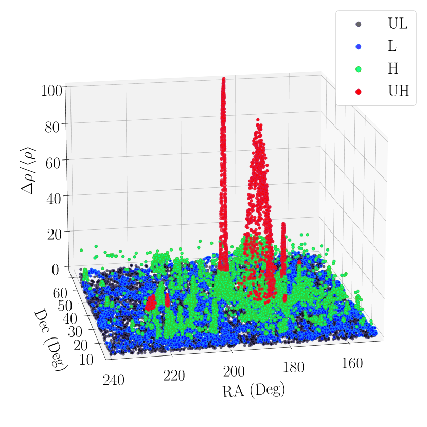
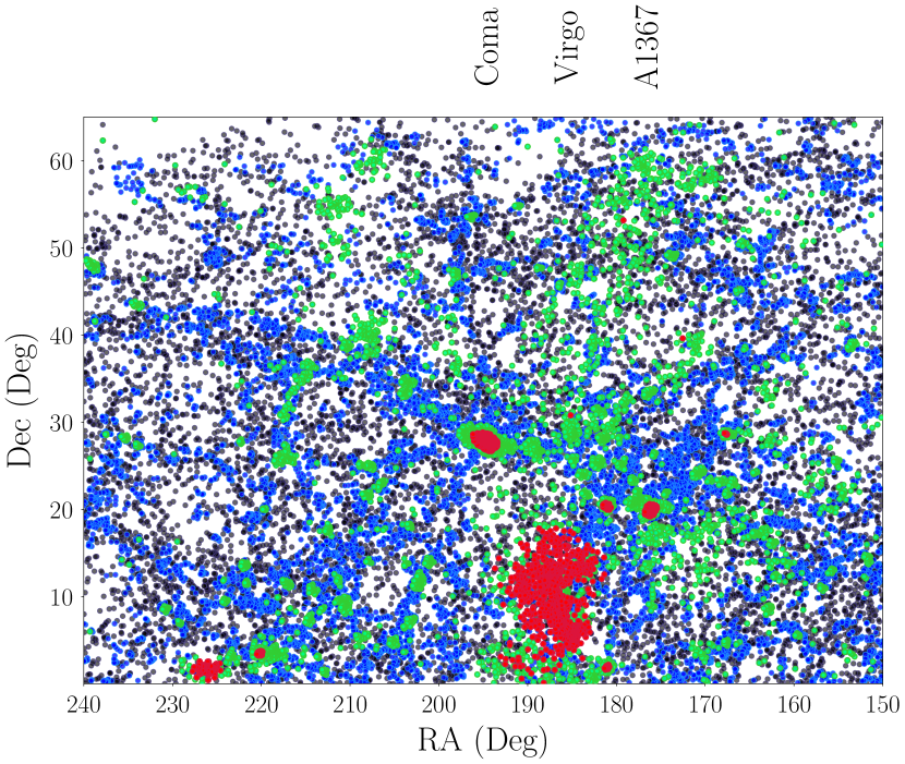
Figure 1: Celestial distribution of the 30597 galaxies analysed in the SPRING catalogue, distributed over nearly one-fourth of the Northern sky. They represent the totality of galaxies in the spring sky within $cz<10000\ \mathrm{km\ s}^{-1}$ and $r<17.7$ mag. The colors represent the overdensity parameter $\Delta\rho/\langle\rho\rangle$ (defined in Sec. $\S$ 2.3.1) for galaxies in four bins of local galaxy overdensity (red = UH, green = H, blue = L, black = UL). On the left panel, the third dimension emphasizes the overdensity parameter. The highest narrow peak represents the Coma cluster, the second narrow peak is A1367, and the broader peak is Virgo.

Since a number of galaxies in the ELP/NSA tables have their photometry taken in off-nuclear positions, their given magnitudes are sometimes not representative of the whole galaxy. For those objects, we re-measure the $u,g,r,i,z$ magnitudes at the central position using the SDSS navigator. For a small subsample of the SPRING catalogue (6764, 22%), we collect information on the precise morphological type from Gavazzi et al. (2003), which were determined after the visual inspection of GOLDMine images.

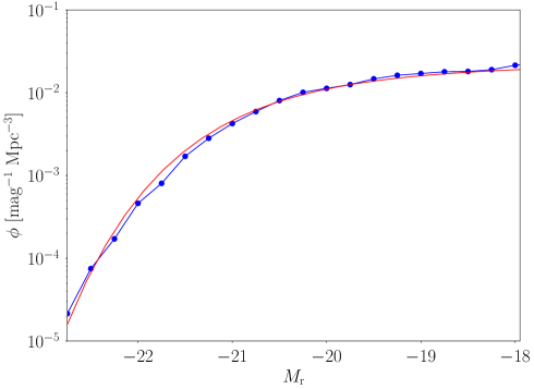
Figure 2: Luminosity function of SPRING galaxies in the $r$-band (blue dots and line). Our best-fitting Schechter function (red line) agrees well with the data points.

The optical and UV data are corrected for Galactic extinction and dust attenuation. For this purpose, we cross-correlate the SPRING sample with the NASA’s Wide-field Infrared Survey Explorer (WISE, Wright et al. 2010) and extracted 22 $\mu$m W4 band data to quantify the attenuation in the FUV and NUV bands following the methods of Boselli et al. (2014) (see also Hao et al. 2011). W4 band data are available for 30373 objects. For galaxies without WISE 22$\mu$m data (224 objects), we estimated the internal attenuation using the mean value derived for objects of similar stellar mass using the relation:

$$A_{\mathrm{NUV}}[\mathrm{mag}]=0.111\times(\log M_{\mathrm{star}})^{2}-1.555\times\log M_{\mathrm{star}}+5.444$$ (1)

calibrated for the star forming galaxies on the rest of the sample. This relation was applied to the blue galaxies ($FUV-i$ $<$ 6) without WISE data, whereas we assumed $A(NUV)$ = 0 mag for the red (presumebly early-type) systems.

The adopted values of the stellar-mass are calculated by the $g$ and $i$ (corrected) magnitudes and the $i$-band luminosity assuming a Chabrier IMF Chabrier (2003) and following the prescription of Zibetti et al. (2009) as:

$$\log(M_{\mathrm{star}}/\mathrm{M}_{\odot})=-0.963+1.032(g-i)+\log l_{I},$$ (2)

where $g$, $i$ are the corrected $g$-band and $i$-band magnitudes, $l_{I}$ is the $i$-band luminosity computed as $\log l_{I}=(I-4.56)/(-2.5)$, and $I$ is the absolute $i$-band magnitude (since our catalog is limited to very low redshift ($z\lesssim 0.03$, no $K$-correction is applied). When the $g$ and $i$ magnitudes are not available, we employ the B and V magnitudes instead, and calculate the stellar-mass as

$$\log(M_{\mathrm{star}}/\mathrm{M}_{\odot})=-1.075+1.837(B-V)+\log l_{V}.$$ (3)

The SPRING catalogue has been cross-matched with H I-data from the GOLDMine database (GM, Gavazzi et al. 2003), the Westerbork Coma Survey (WCS, Molnár et al. 2022), the ALFALFA survey (AA, Haynes et al. 2011; Durbala et al. 2020), and the HyperLeda catalogue Makarov et al. (2014). We cross-match our sample by coordinates separation with the criteria $c\delta z<200$ km s^-1 (for all datasets), $\delta\theta<5^{{}^{\prime\prime}}$ for GM, AA, and WSB and $\delta\theta<10^{{}^{\prime\prime}}$ for LEDA. This choice was motivated by the lower accuracy of LEDA celestial coordinates; non-unique associations were visually inspected. H I data are available for 9461 objects ($\sim$30%). If H I-data from more than one source are available, we select data taken from GM over WCS, AA, and LEDA, respectively. This choice is motivated by (i) the higher sensitivity of GM/WCS over AA, and (ii) the inhomogeneity in LEDA sources, which were listed across a wide time span with diverse methodology.

A widely adopted method to identify galaxies at different evolutionary stages is the colour-stellar-mass relation Boselli et al. (2008, 2014); Hughes & Cortese (2009); Cortese & Hughes (2009); Gavazzi et al. (2010). We use the $\mathrm{NUV}-i$ vs $M_{\mathrm{star}}$ relation Kennicutt (1998) as a tracer of the mean age of the stellar population of galaxies in our sample, which we separate into three “chromatic” classes: (i) a red sequence, composed of quiescent ETGs; (ii) a blue cloud of star-forming LTGs Gil de Paz et al. (2007); (iii) and a green valley separating these two sequences Martin et al. (2007). We identify the red sequence as the region in the $(\mathrm{NUV}-i)$ vs $M_{\mathrm{star}}$ plane for which $\mathrm{NUV}-i>0.47\log M_{\mathrm{star}}+0.1$; the blue cloud is the region for which $\mathrm{NUV}-i<0.47\log M_{\mathrm{star}}-1.0$; the green valley is the region between the former two. This representation, chosen by Boselli et al. (2014) to study the Virgo cluster, is here extended to a much larger ($\sim 30\times$) sample.

2.2 Nuclear spectra

Besides the SDSS, several other sources of nuclear spectroscopy are available in the literature; we integrate the SDSS spectroscopic data (available for 28971 targets) with two extensive spectral surveys: the one by Ho et al. (1993, 1995, 1997) undertaken with the Palomar 200 inch telescope (224 spectra added), and the one by Falco et al. (1999) using the Tillinghast 1.5m telescope (366 spectra added).

On our side, since 2005 we undertook a spectroscopic project using the $\mathrm{Cassini}1.5\mathrm{m}$ telescope of the Loiano Observatory aiming at integrating the SDSS with the nuclear spectroscopy of galaxies in the local Universe Gavazzi et al. (2011, 2013a). In 2014-2020, we obtained 302 new nuclear spectra (see Appendix A). These spectra are generally taken with the red-channel of the spectrograph, namely between 6000 and 8000 Å; only a dozen galaxies were observed also with the blue grism. In addition, five spectra were taken with the MUSE IFU by Consolandi et al. (2017); Fossati et al. (2019); Pedrini et al. (2022). Altogether, the total number of galaxies with nuclear spectra observed independently from SDSS is 884.

All entries (images and spectra) in the SPRING catalogue were individually inspected in search of errors (e.g., false objects caused by diffraction spikes of bright stars, duplicates, misclassified objects). This initial iterative examination led us to clear $\sim$1% of the objects in our sample; also, the direct inspection of all targets using the SDSS navigator tool (DR13 version) allowed us to eliminate 74 (less than 0.3 %) targets with more than one spectrum available (i.e., galaxies with two or more nuclear spectra and galaxies with non-nuclear spectra). We leave two entries for the same object only in obvious post-merger targets where two nuclei are visible.

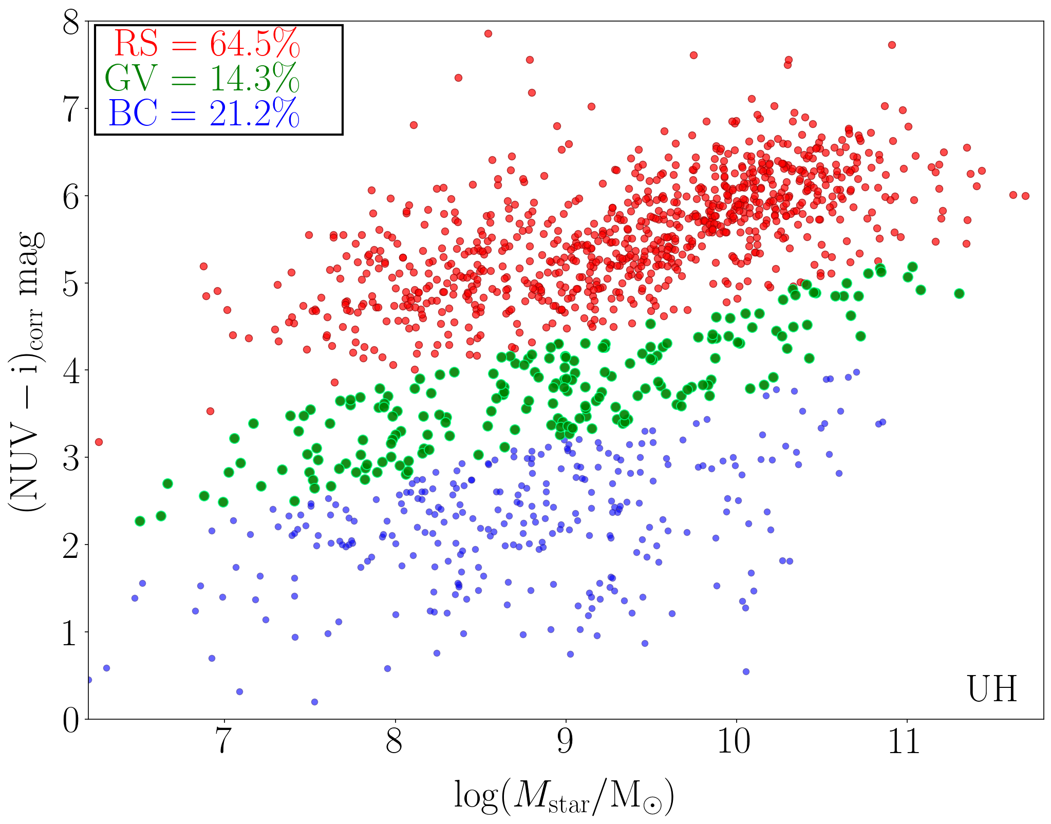
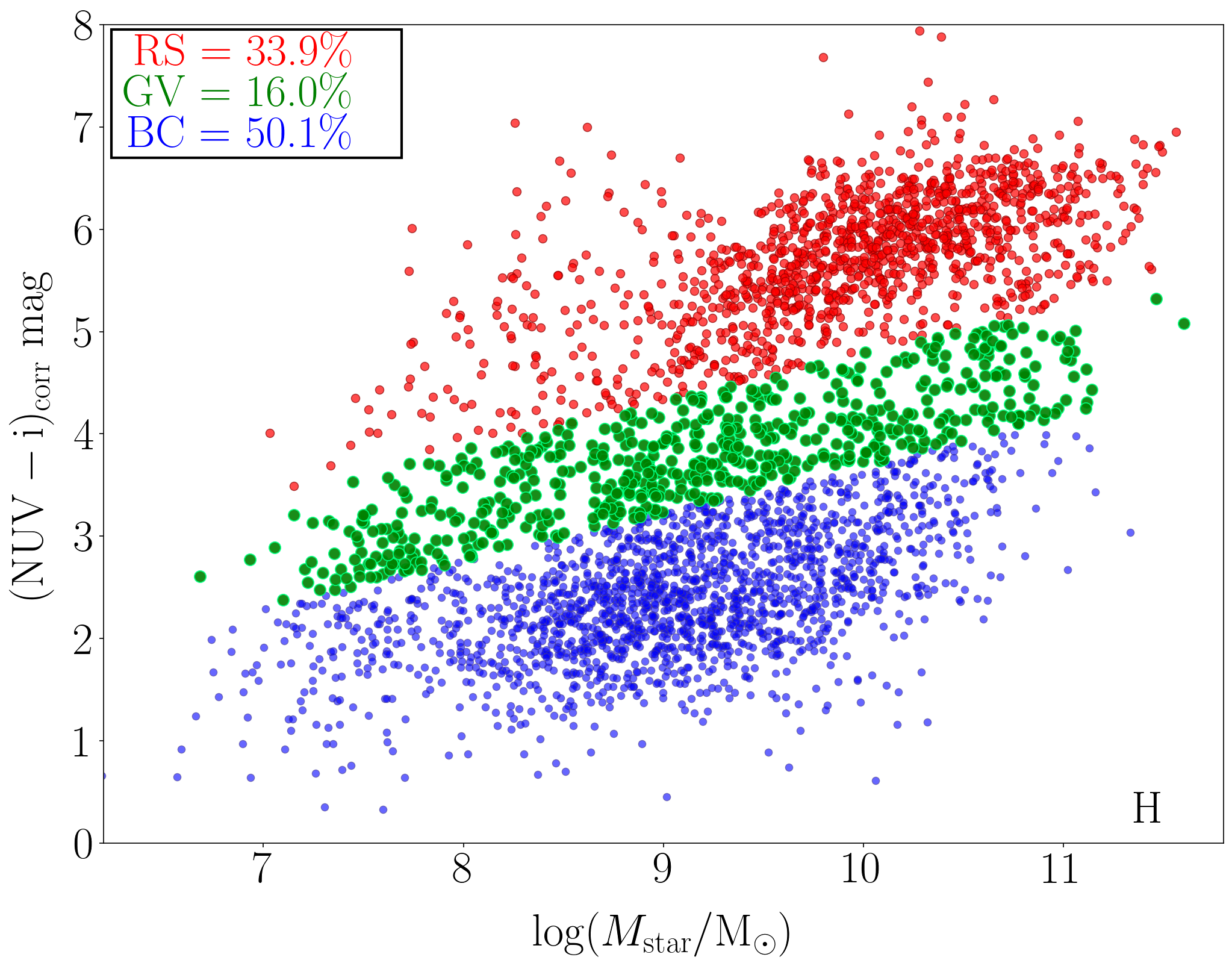
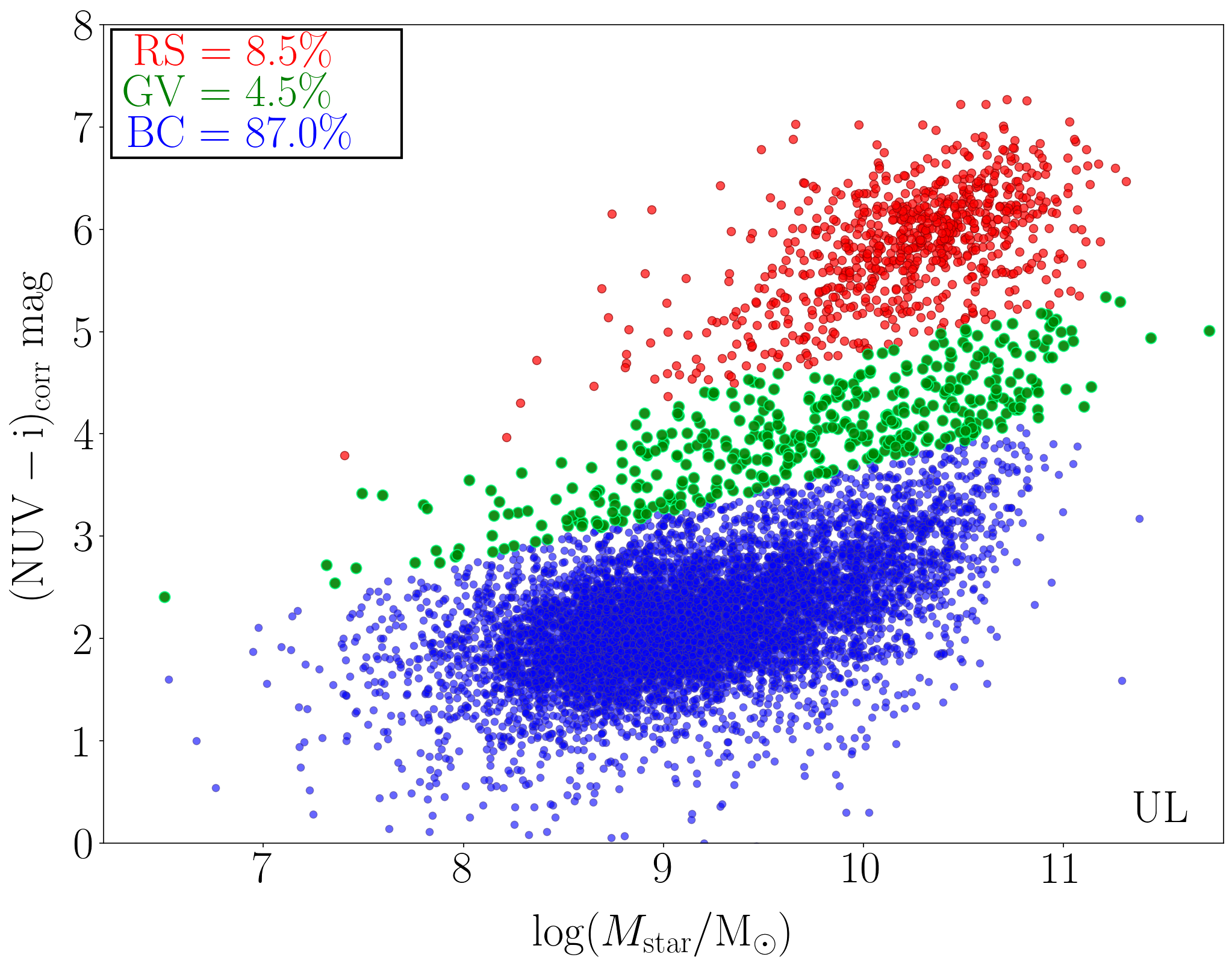
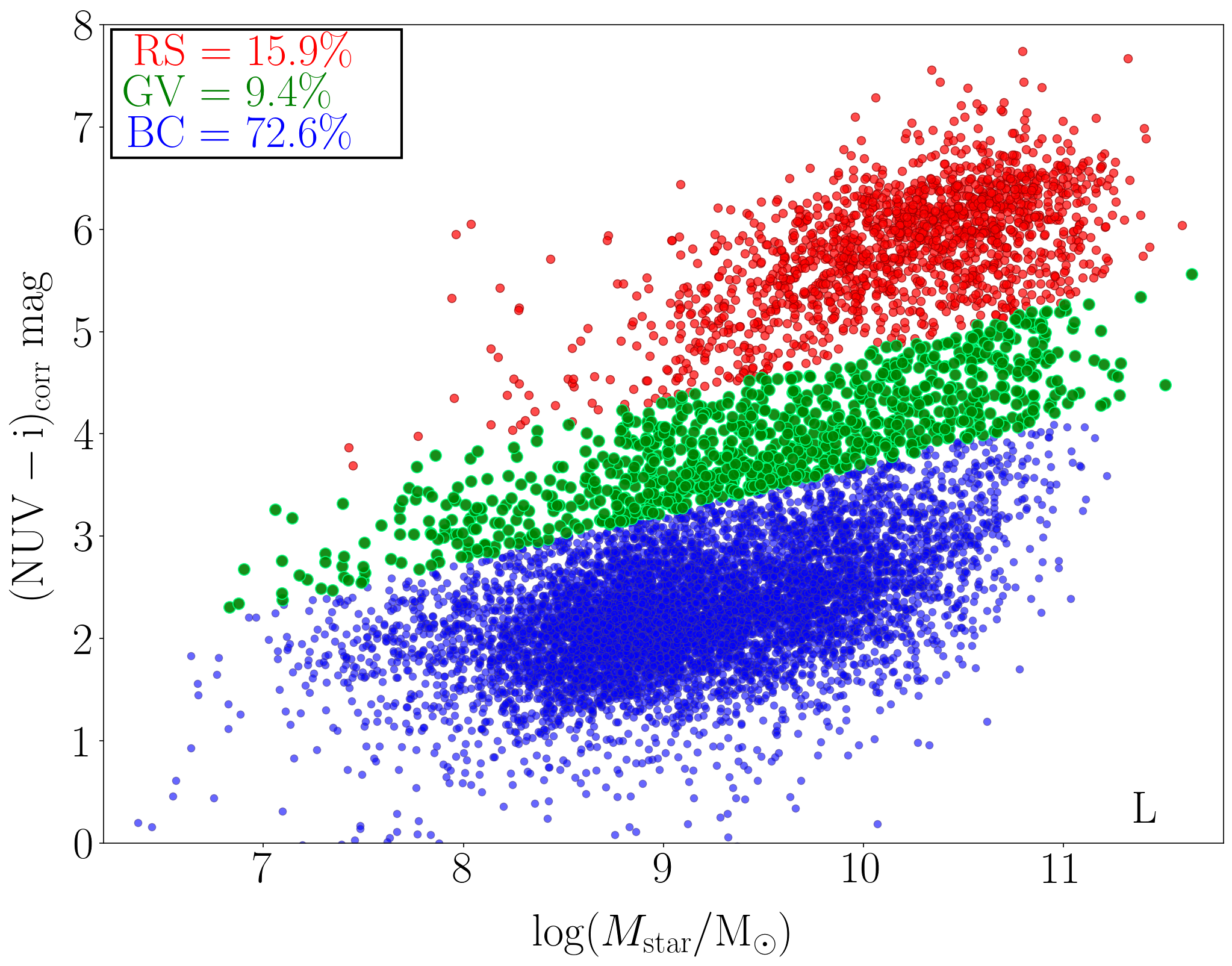
Figure 3: Corrected $\mathrm{NUV}-i$ colour versus stellar-mass diagram relation of all galaxies in this sample divided in blue cloud (BC), green valley (GV), and red sequence (RS), according to the chromatic criterion of Boselli et al. (2014) (see Sec. $\S$ 2.1), in four bins of galaxy overdensity (from UH to UL clockwise from top left). In each panel (corresponding to the four overdensities) are reported the fractions of galaxies in the three chromatic classes with respect to the total number of galaxies in the corresponding overdensity bin.

The SPRING catalogue is limited to $cz<$10000 km s^-1. Up to this redshift, corresponding to a distance of $\sim$137$h^{-1}$ Mpc and embracing a volume of 780000$h^{-3}$ Mpc³, the sample is volume- and magnitude-limited, thus the number counts in bins of $M_{\mathrm{star}}<10^{9}\ \mathrm{M}_{\odot}$ (or $r<-17.7$ mag) can be converted into mass/luminosity functions. We verify that the $r$–band luminosity function (LF) of our sample matches that derived by Blanton et al. (2001) (including normalization, $M_{\mathrm{knee}}$ and slope). To this extent, we compare our galaxy distribution in the $r$-band magnitude space to a galaxy LF model using a maximum likelihood model (Fig. 2). We adopt a Schechter function Schechter (1976) and find the best-fit parameters $\alpha=-1.08,M^{*}=20.64,\phi_{*}=2.1\cdot 10^{-2}$; the normalized mean residual between the fit and out data is $\sim 0.28$ dex.

2.3 Probing the galaxy environment

Our analysis of the environmental properties of SPRING galaxies relies on differing techniques: in §2.3.1, we reconstruct the 3D distribution of $\sim$30000 galaxies in 5400 square degrees of the spring sky and determine the density around each galaxy measuring the number of neighbors within fixed cylindrical volumes; in §2.3.2, we adopt the halo-mass as a tracer of the galaxy environment; in §2.3.3, we employ the H I-deficiency parameter to investigate the H I-content distribution of galaxies.

2.3.1 Galaxy density

The local galaxy density around each object is quantified according to the method of Gavazzi et al. (2010) which we briefly summarise in the following. After reducing the fingers of God of the three major clusters by collapsing the individual galaxy velocities to the average cluster velocity $\langle cz\rangle$, the density $\rho$ was determined in cylinders of 1$h^{-1}$ Mpc radius and 1000 km s^-1 half-length. Given an average density $\langle\rho\rangle$ of 0.04 gal $h^{3}$ $\text{Mpc}^{-3}$, the resulting overdensity parameter $(\rho-\langle\rho\rangle)/\langle\rho\rangle\equiv\Delta\rho/\langle\rho\rangle$ is estimated. This procedure is applied to all galaxies with a distance greater than 15$h^{-1}$ Mpc, to exclude very local galaxies which can be subject to large distance uncertainties due to peculiar velocities; 879 local galaxies are thus excluded from our overdensity determination. Following Gavazzi et al. (2010), we define four arbitrary overdensity thresholds which are chosen to highlight increasing levels of aggregation:

1. Ultra low (UL): $\ \ \ \ \ \ \ \ \ \ \ \ \ \ \ \ \Delta\rho/\langle\rho\rangle\leq 0$

2. Low (L): $\ \ \ \ \ \ \ \ \ \ \ \ \ \ \ \ \ \ \ \ 0<\Delta\rho/\langle\rho\rangle\leq 4$

3. High (H): $\ \ \ \ \ \ \ \ \ \ \ \ \ \ \ \ \ \ \ 4<\Delta\rho/\langle\rho\rangle\leq 20$

4. Ultra High (UH): $\ \ \ \ \ \ \ \ \ \ \ \ \ \ \Delta\rho/\langle\rho\rangle>20$.

The UL density bin describes the underlying cosmic web; the L density bin is for the loose groups and the filaments in the Great Wall; the H bin includes the significant groups and cluster outskirts; the UH bin represents the cores of the clusters. Figure 1 shows the overdensity parameter distribution in the whole sample.

To check the qualitative consistency with the morphology-segregation effect observed by Dressler (1980), we derive that the fraction of galaxies in the red sequence over the total in the four different density bins is 7% in UL, 14% in L, 29% in H and 59% in UH. In addition, to check consistency with Gavazzi et al. (2010) (see Fig. 8 therein), we use the colour-stellar-mass relation to study the variation of the chromatic distribution with increasing overdensity parameter. Figure 3 displays four NUV-$i$ vs stellar-mass diagrams, highlighting the chromatic distributions of galaxies in the four overdensity bins. For each panel, the fractions of galaxies in the blue cloud, green valley, and red sequence are reported.

We observe that low-mass galaxies in the blue cloud dominate the population of galaxies in the UL bin ($\sim$86%); still, there is a significant contribution of galaxies in the red sequence (and, to a lesser extent, in the green valley) which is, however, restricted to the larger ($M_{\rm star}>10^{9.5}$ M_⊙) masses. Conversely, in the UH bin, there is a minimal contribution of blue-cloud galaxies altogether ($\sim$20%), and the red sequence includes a significant population of dwarf galaxies.

2.3.2 Halo-mass

An alternative, widely used method to evaluate a galaxy’s environment is by the halo-mass of the group to which it belongs (see, e.g., Muldrew et al. 2012; Fossati et al. 2015). The halo-mass is obtained from abundance matching techniques between the halo-mass function and the stellar-mass (or luminosity) of the most-massive galaxy identified within the group (see e.g., Yang et al. 2007, 2008, 2009). We correlate our $cz<10000$ km s^-1 catalogue with the one by Yang et al. (2007), which extends much further out than our local sample, however excluding the Local Supercluster and the Virgo cluster ($cz>3000$ km s^-1). We find 21608 matches in the shared redshift range between the two catalogues.

Only 427 galaxies in the Yang catalogue have no counterpart in our database, and a visual inspection revealed them to be primarily extranuclear H II regions, not galactic nuclei. For the galaxies in common, we take the group halo-mass estimate obtained from the total stellar-mass in the group. For the Virgo cluster, which is not present in Yang et al. (2007) and thus does not have an estimate of the virial mass, we use the estimate ($M_{200}=10^{14.4}\rm{M}_{\odot}$) reported by Boselli & Gavazzi (2006).

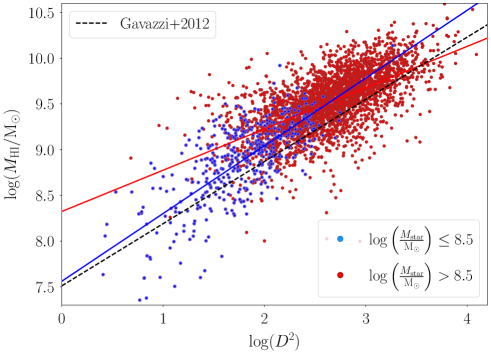
Figure 4: $\log(M(\mathrm{H}\thinspace\scriptsize{\text{I}}))$ vs $\log(D^{2})$ distribution of galaxies belonging to the UL overdensity bin and with $\log(M_{\mathrm{star}}/\mathrm{M}_{\odot})\leq 8.5$ (blue dots), and $\log(M_{\mathrm{star}}/\mathrm{M}_{\odot})>8.5$ (red dots). The colour straight lines denote the best-fit linear regression in each mass bin, whose coefficients are given in Table 1. The black dashed line denotes the linear fit given in Gavazzi et al. (2013b).

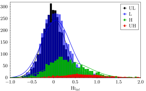
Figure 5: Distribution of the newly calibrated $\mathrm{H}\thinspace\scriptsize{\text{I}}_{\mathrm{def}}$ parameter in four bins of galaxy overdensity. The mean values and standard deviations for each overdensity bin are given in Table 2.

In analogy with the overdensity parameter, we define 3 halo-mass ranges:

1. Low (L): $\ \ \ \ \ \ \ \ \ \ \ \ \ \ \ \ \ \ \ \ \ \ \ \ \ \ \ \ \ \ \ \ \log(M_{\mathrm{halo}}/\mathrm{M}_{\odot})\leq 12.5$

2. Intermediate (M): $\ \ \ \ \ \ 12.5<\log(M_{\mathrm{halo}}/\mathrm{M}_{\odot})\leq 13.5$

3. High (H): $\ \ \ \ \ \ \ \ \ \ \ \ \ \ \ \ \ \ \ \ \ \ \ \ \ \ \ \ \ \ \ \log(M_{\mathrm{halo}}/\mathrm{M}_{\odot})>13.5$

2.3.3 H I-deficiency

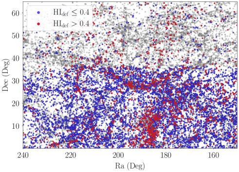
Figure 6: Sky distribution of galaxies in the SPRING sample in classes of HI-deficiency parameter. The horizontal line at $\mathrm{Dec}=36\ \mathrm{deg}$ traces the limiting pointing declination of the Arecibo dish. Grey circles stand for galaxies for which the H I content is unknown. Blue dots denote galaxies with H I${}_{\mathrm{def}}\leq 0.4$, while red dots are for galaxies with H I${}_{\mathrm{def}}>0.4$. The latter class is distributed consistently around (in) the Coma cluster and the Virgo cluster, with a small number of entries belonging to the A1367 cluster. It is noticeable that our knowledge of the H I properties of local galaxies in such an extended stretch of the sky depends on the availability of Arecibo data, which are limited to Declination $\lesssim$ 36^∘.

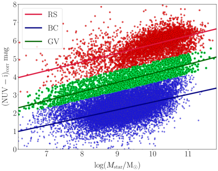
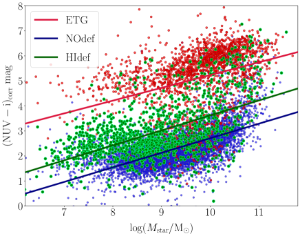
Figure 7: Left: corrected $\mathrm{NUV}-i$ colour versus stellar-mass diagram relation of all galaxies in this sample divided according to the chromatic criterion of Boselli et al. (2014) (see Fig. 2 therein) whether they belong to the red sequence (RS), the green valley (GV) or the blue cloud (BC). For each class, the linear regression analysis is given. Right: the same relation for the subsample of ETGs with detailed morphological classification available (red); of deficient (H I$>0.4$, green) and non-deficient galaxies (H I$\leq 0.4$, blue). The slopes of the linear regressions for the ETGs and the H I-deficiency classes are consistent with the ones corresponding to the three chromatic classes. The NUV and $i$ magnitudes are corrected for dust attenuation (see Boselli et al. 2014).

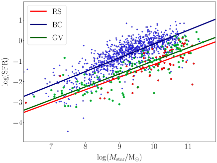
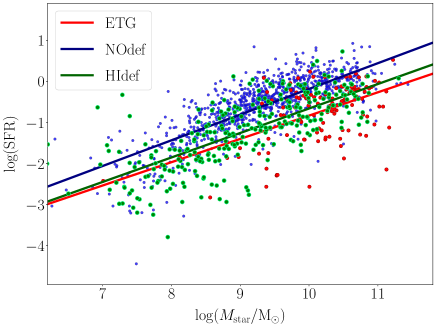
Figure 8: Left: main sequence relation of all galaxies in this sample divided according to the chromatic criterion of Boselli et al. (2014) (see Fig. 2 therein) whether they belong to the red sequence (RS), the green valley (GV) or the blue cloud (BC). For each class, the linear regression analysis is given. Right: the same relation for the subsample of ETGs with detailed morphological classification available (red); of deficient (H I$>0.4$, green) and non-deficient galaxies (H I$\leq 0.4$, blue). The slopes of the linear regressions for the ETGs and the H I-deficiency classes are consistent with the ones corresponding to the three chromatic classes.

A third method for investigating environmental effects is studying the atomic Hydrogen (H I) content of galaxies, because galaxies in clusters are H I-deficient compared to galaxies in lower density environments. H I-observations provide powerful diagnostics of the role of the environment in regulating the evolution of late-type galaxies in the local Universe Gavazzi et al. (2012, 2013b, 2013c); Fossati et al. (2013); Gavazzi et al. (2015b, a). In the present work, we employ ALFALFA (AA, Durbala et al. 2020), GOLDMine (GM, Gavazzi et al. 2003), the Westerbork Coma Survey (WCS, Molnár et al. 2022), and the HyperLeda catalogue (LEDA, Makarov et al. 2014) H I 21 cm line data to estimate the H I-deficiency parameter $\mathrm{H}\thinspace\scriptsize{\text{I}}_{\mathrm{def}}$, defined as Haynes & Giovanelli (1984); Giovanelli & Haynes (1985); Gavazzi et al. (2003)

$$\mathrm{H}\thinspace\scriptsize{\text{I}}_{\mathrm{def}}=\log M(\mathrm{H}\thinspace\scriptsize{\text{I}})_{D}-\log M(\mathrm{H}\thinspace\scriptsize{\text{I}})_{\mathrm{obs}},$$ (4)

where $\log M(\mathrm{H}\thinspace\scriptsize{\text{I}})_{D}$ is the H I-mass computed as a function of the optical linear diameter $D$ Meyer et al. (2017) as

$$\log M(\mathrm{H}\thinspace\scriptsize{\text{I}})_{D}=C_{1}+C_{2}\log(D^{2}).$$ (5)

The coefficients $C_{1}$ and $C_{2}$ are empirically determined by studying a control sample of isolated objects (see, e.g., Haynes & Giovanelli 1984; Gavazzi et al. 2013b). The SPRING catalogue includes 9461 galaxies with H I data from GM, WCS, AA, and LEDA. When data from more than one catalogue are available, we choose GM data over WCS, AA, and LEDA, respectively. The diameters of this subset of galaxies are retrieved from NED. Since our HI data are taken from surveys with different limiting sensitivities, our HI-mass determination only includes detections and no upper limits.

As discussed in Cortese et al. (2021), there are different methods which can be employed to quantify the H I-deficiency parameter. We perform a recalibration of the optical diameter-based H I-deficiency parameter employing a reference sample of isolated galaxies corresponding to the UL overdensity bin of our catalogue containing 11051 objects, among which 3416 have H I data. We find that the slope of the $\log(M(\mathrm{H}\thinspace\scriptsize{\text{I}}))$ vs $\log(D^{2})$ relation is strongly dependent on the galaxy stellar-mass; in contrast, no significant discrepancy in the linear fits for different morphological types is observed. To further investigate the stellar-mass dependence, we divide the galaxies in our sample in six bins of stellar-mass (dubbed as M1,…,M6) defined as

• M1:             log($M_{\mathrm{star}}/\mathrm{M}_{\odot})\leq 8.5$;

• M2:  8.5 $<$ log($M_{\mathrm{star}}/\mathrm{M}_{\odot})\leq 9$;

• M3:     9 $<$ log($M_{\mathrm{star}}/\mathrm{M}_{\odot})\leq 9.5$;

• M4:  9.5 $<$ log($M_{\mathrm{star}}/\mathrm{M}_{\odot})\leq 10$;

• M5:    10 $<$ log($M_{\mathrm{star}}/\mathrm{M}_{\odot})\leq 10.5$;

• M6:             log($M_{\mathrm{star}}/\mathrm{M}_{\odot})>10.5$.

For each stellar-mass bin, we study individually the $\log(M(\mathrm{H}\thinspace\scriptsize{\text{I}}))$ vs $\log(D^{2})$ relation and find that the slope of M1 galaxies ($\log\left(M_{\mathrm{star}}/\mathrm{M}_{\odot}\right)\leq 8.5$) is significantly steeper than that of galaxies in larger stellar-mass bins (see Fig. 4). The values of the best-linear fit coefficients $C_{1}$ and $C_{2}$ in the two mass bins are reported in Table 1. The histogram in Fig. 5 displays the distribution of our parametrization for the H I-deficiency parameter of the galaxies in our sample divided in overdensity bins. In Table 2 we give the mean values and the standard deviations of Gaussian fits to the $\mathrm{H}\thinspace\scriptsize{\text{I}}_{\mathrm{def}}$ distribution in each overdensity bin. We observe that the mean value of $\mathrm{H}\thinspace\scriptsize{\text{I}}_{\mathrm{def}}$ increases as we move from isolated galaxies (UL bin, $\langle\mathrm{H}\thinspace\scriptsize{\text{I}}_{\mathrm{def}}\rangle\sim 0$) to galaxies in the centre of clusters (UH bin, $\langle\mathrm{H}\thinspace\scriptsize{\text{I}}_{\mathrm{def}}\rangle\sim 0.7$).

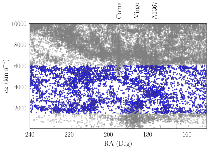
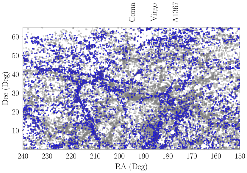
Figure 9: Left: Distribution of the Hubble velocity $cz$ as a function of RA in the spring sky to illustrate the criterion discussed in Sec. §2.4 (1500 ¡ $cz/\mathrm{km\ s}^{-1}$¡ 6000, excluding objects belonging to the fingers of God of either Coma or Virgo). Right: sky distribution of galaxies in the 1500 ¡ $cz/\mathrm{km\ s}^{-1}$¡ 6000 range displaying the existence of a filamentary structure that we dub the Spring Ring.

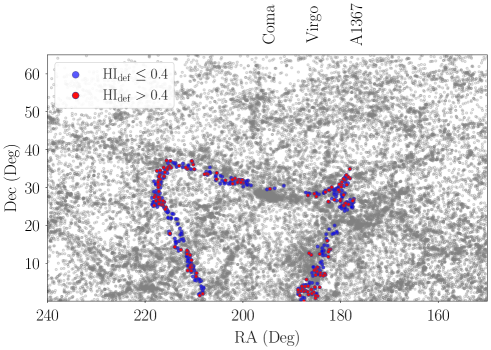
Figure 10: The sky distribution of galaxies belonging to the Spring Ring in two bins of H I deficiency parameter $\mathrm{H}\thinspace\scriptsize{\text{I}}_{\mathrm{def}}\leq 0.4$ (blue) and $\mathrm{H}\thinspace\scriptsize{\text{I}}_{\mathrm{def}}>0.4$ (red).

Figure 11: The sky distribution of the 515 galaxies belonging to the Spring ring and having H I data. The third dimension is given by the Hubble velocity $cz$. The color map displays the $\mathrm{H}\thinspace\scriptsize{\text{I}}_{\mathrm{def}}$ parameter.

Table 1: Coefficients of the $\log(M(\mathrm{H}\thinspace\scriptsize{\text{I}}))$ vs $\log(D^{2})$ relation for the two stellar-mass bins M1 ($\log\left(M_{\mathrm{star}}/\mathrm{M}_{\odot}\right)\leq 8.5$) and M2-M6 ($\log\left(M_{\mathrm{star}}/\mathrm{M}_{\odot}\right)>8.5$).

Stellar-mass		$C_{1}$	$C_{2}$
$\log\left(M_{\mathrm{star}}/\mathrm{M}_{\odot}\right)\leq 8.5$		5.10	0.73
$\log\left(M_{\mathrm{star}}/\mathrm{M}_{\odot}\right)>8.5$		6.98	0.42

We classify galaxies as deficient (non-deficient) if $\mathrm{H}\thinspace\scriptsize{\text{I}}_{\mathrm{def}}>0.4$ ($\mathrm{H}\thinspace\scriptsize{\text{I}}_{\mathrm{def}}\leq 0.4$). The $\mathrm{H}\thinspace\scriptsize{\text{I}}_{\mathrm{def}}$ parameter is a proxy for the influence of the environment on the neutral Hydrogen content of galaxies (in fact, it significantly correlates with our overdensity parameter $\Delta\rho/\langle\rho\rangle$).

Table 2: Mean value and standard deviation of the Gaussian fits for the H I-deficiency distributions in each overdensity bin.

Overdensity		Mean	$\sigma$
UL		0.00	0.26
L		0.04	0.32
H		0.24	0.41
UH		0.64	0.52

Our sample contains three rich clusters (Coma, A1367 and Virgo, see Figure 1), thus it includes a significant number of H I-deficient objects (see Figure 6). Since the deficiency parameter depends on the distance, AA detects galaxies with $\mathrm{H}\thinspace\scriptsize{\text{I}}_{\mathrm{def}}\gtrsim 0.3$ in the Local Supercluster, but it only manages to detect galaxies with normal H I content at the distance of Coma. The detection of deficient galaxies in Coma and A1367 requires more sensitive observations than those by AA, such as those by GM or WCS.

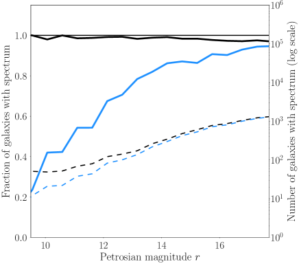
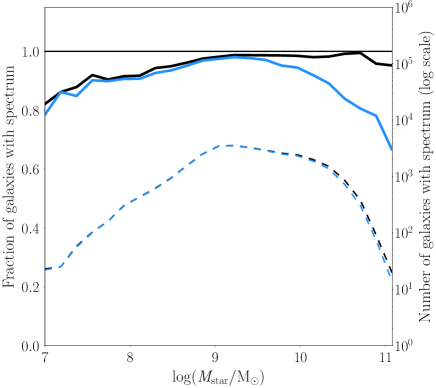
Figure 12: Completeness (defined as the fraction of galaxies with nuclear spectra over the total number of galaxies, left axis and thick straight lines) and actual number of galaxies with nuclear spectra (right axis and dashed lines) as a function of $r$ apparent magnitude (top) and as a function of stellar-mass (bottom). The blue lines represent SDSS-only spectra, the black lines include spectra taken from the SDSS and other sources.

Using different symbols (and colours) for the non-deficient galaxies ($\mathrm{H}\thinspace\scriptsize{\text{I}}_{\mathrm{def}}\leq 0.4$, blue), for the deficient galaxies ($\mathrm{H}\thinspace\scriptsize{\text{I}}_{\mathrm{def}}>0.4$, green) and for early-type galaxies whose detailed morphological information is available from Gavazzi et al. (2003) (red), we show the dependence of the $\mathrm{NUV}-i$ colour on the stellar-mass (see Fig. 7, right panel).

Along with the subsets of galaxies coded by H I-content, we chose to display ETGs to highlight the correspondence between the three classes (ETGs, HIdef, non-HIdef) and the chromatic classification (red sequence, green valley, blue cloud).

We observe that our chromatic classification is closely related to the content of H I, as the slopes of the H I-deficient and H I-normal galaxies in the color-mass diagram (Fig. 7, right) parallel those of the three colour classes representation (Fig. 7, left) which was chosen by Boselli et al. (2014) to study the Virgo cluster. The similarity between the classes of H I-content and the BC and GV chromatic classes is visible also in the main sequence (i.e., SFR vs stellar-mass) relation. We cross-match our catalogue with the $H\alpha 3$ catalogue (Gavazzi et al. 2012, 1396 galaxies in common), from which we extract the star formation rate which is derived from observed, integrated $H\alpha$ flux after applying correction for (i) Galactic extinction (assuming the extinction law by Cardelli et al. 1989), (ii) [NII] contamination in the narrow-band imaging filter, and (iii) internal extinction, this last estimated as described in Gavazzi et al. (2012) (see also Fossati et al. 2013; Gavazzi et al. 2015b, a). Figure 8 shows the main sequence relation for this subset of galaxies coded according to their H I-content (right) and their chromatic classification (left). We observe that H I-deficient galaxies display lower SFR than H I-normal objects of the same stellar-mass, suggesting that the lack of H I gas leads to a reduction in the activity of star formation Boselli et al. (2022).

2.4 The Spring Ring

As shown in Fig. 6, deficient objects are mostly distributed in clusters. The fraction of objects with $\mathrm{H}\thinspace\scriptsize{\text{I}}_{\mathrm{def}}>0.4$ in the three clusters Virgo, Coma, and A1367 is $\sim 62.4\%$. In addition, we observe that a consistent fraction of deficient galaxies is distributed in filamentary structures. To further investigate the significance of this finding, we select galaxies at intermediate distances (velocities) between Virgo and Coma (1500 ¡ $cz/\mathrm{km\ s}^{-1}$¡ 6000), excluding objects belonging to the fingers of God of either Coma or Virgo (see Fig. 9, left panel). A total of 6095 objects are selected this way. In addition, we remove from this selection 194 objects belonging to the highest (UH) overdensity bin. The celestial distribution of 5911 galaxies selected with this criterion is given in Fig. 9 (right panel), showing the existence of a definite filamentary structure which we dub the “Spring Ring” (SR). We manually isolate galaxies in the ring to study their H I-content. Two- and three-dimensional sky distributions of this structure are given in Figs. 10-11. We identify four main branches within the SR, denoted with fA, fB, fC, and fD in the figures. The fA branch displays evidence of gravitational influence from the Virgo cluster; fB is made by galaxies which show hints of gravitational attraction from A1367; fC comprises galaxies infalling toward the Coma cluster; fD does not exhibit signs of influence from one of the three clusters considered in the present work.

The Spring Ring is mostly composed of blue-cloud galaxies ($\sim 80\%$) with stellar-mass $M_{\rm star}\lesssim 10^{10}$ M_⊙. Remarkably, when we divide galaxies with H I data belonging to the SR (515 entries) among H I-deficient and H I-normal objects, we find that 158 ($\sim$30.7%) of them are H I-deficient (see Figs. 10-11). Conversely, the fraction of H I-deficient objects among field galaxies (i.e., SPRING galaxies that do not belong to the UH overdensity bin) is $\sim$12%. We cross-matched these 515 SR galaxies with the recent catalogue by Castignani et al. (2022b). We find that 143 galaxies in the SR are reported also in Castignani et al. (2022b). Among these, the most noticeable fractions are found among galaxies belonging to the W-M sheet (57 entries), the NGC5353_4 filament (41), and the Coma Berenices filament (29). It is noticeable that the majority of the left branch of the SR is not identified in Castignani et al. (2022b).

To accurately compare the fraction of H I-deficient objects in the filament to the general population, we randomly select a sample of 515 objects from the galaxies in the SPRING sample which have H I data, and count the fraction of H I-deficient objects. We repeat this procedure ten thousand times, and find that the fraction of $\mathrm{H}\thinspace\scriptsize{\text{I}}_{\mathrm{def}}$ galaxies is (16.7 $\pm$ 1.6)%.

In addition, we investigate whether the fraction of H I-deficient objects in the SR is related to the distribution of galaxy overdensity within the filamentary structure; to this end, we randomly select ten thousand overdensity-matched samples of 515 galaxies with H I data (i.e., the overdensity parameter distribution of each random sample matches the overdensity distribution within the SR). We find that (20.2 $\pm$ 1.6)% galaxies in the matched-samples are H I-deficient. This value is larger than the fraction found in the random samples with no restriction on the overdensity distribution (20.2% vs 16.7%). Still, it is considerably smaller than the fraction of deficient objects found within the SR (30.7%). This result suggests that (i) local galaxies in filamentary structures are more H I-deficient than field galaxies, and (ii) their H I-content does not depend (only) on their local galaxy overdensity.

In the literature, there is controversial evidence regarding the H I-content of filament galaxies. Lee et al. (2021) claims that the H I-content of galaxies in filaments is normal, whereas Castignani et al. (2022a) finds a higher incidence of H I-deficient galaxies in filaments (see, e.g., Fig. 17 in Castignani et al. 2022a). Since galaxies in the SR are mostly low-mass, they have low binding energies and thus can be easily affected by perturbations as they move along the filament. This scenario is consistent with Crone Odekon et al. (2018), who examined a sample of $\sim$4000 LTGs with H I data and found that galaxy H I-content decreases with distance from a filament spine. Multiple mechanisms (e.g., gas-stripping, tidal interaction) may affect filament galaxies before they enter higher-density regions; in Fig. 11, we see that most SR galaxies at the early stage of gas stripping (yellow dots) are found in the fD branch, while galaxies with higher H I-deficiency (purple dots) mostly appear to be falling towards the core of a cluster. In addition, a high fraction of deficient objects is found in the proximity of the intersection between the fD and fC branches.

3 Nuclear Spectral classification

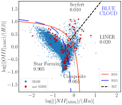
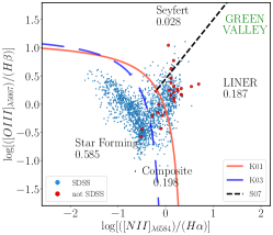
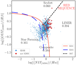
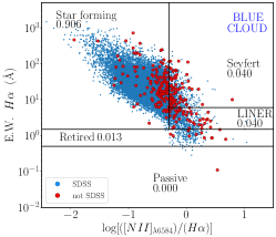
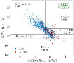
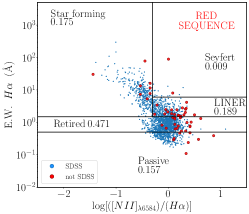
Figure 13: (Top row): The BPT diagnostic diagram for galactic nuclei in the blue cloud, green valley and red sequence (left, centre and right respectively). The SDSS galaxies are given with blue points. Measurements from other sources are given with larger red dots. For each spectral category is given the associated percentage of galaxies. The red straight line represents the model of Kewley et al. (2001) to identify AGN. The blue long-dashed line gives the model of Kauffmann & Haehnelt (2000) above which AGN are found. Composite nuclei fall between these two models. The black dashed line (Schawinski et al. (2007)) separates Seyfert from LINERs. (Bottom row): The WHAN diagnostic diagram for galactic nuclei in the blue cloud, green valley and red sequence (left, centre and right respectively). The SDSS galaxies are given with blue points. Measurements from other sources are given with larger red dots. For each spectral category is given the associated percentage of galaxies.

In this Section, we aim to link the photometric and environmental properties of the galaxies in the SPRING sample with the spectral features of their nuclei. We provide nuclear-emission classification by optical spectra based on two ionisation diagnostic diagrams: (i) the Baldwin-Phillips-Terlevich diagnostic (BPT diagram, Baldwin et al. 1981), and the EWH$\alpha$ vs. [NII]/H$\alpha$ diagram (WHAN, Cid Fernandes et al. 2010, 2011). These diagnostics aim to identify the main ionizing mechanisms in galactic nuclei (e.g., young/old stars, AGN). Out of the total of 30597 entries, we restrict our classification of nuclear activity to spectra having all lines with signal to noise ratio $>3$: we classify 22564 (74%) galaxies of the SPRING catalogue using the BPT, and 24559 galaxies (80%) using the WHAN. To investigate the impact of the inclusion of non-SDSS spectra to our sample, we define the spectral completeness as the fraction of galaxies with nuclear spectra over the total number of galaxies. In Fig. 12, we show the completeness as a function of the $r$-band magnitude (top panel) and of the stellar-mass $\log(M_{\mathrm{star}}/\mathrm{M}_{\odot})$ (bottom panel). The blue lines represent SDSS-only spectra, the black lines include spectra taken from the SDSS and other sources. Along with the completeness of the SPRING catalogue compared to SDSS-only data (thick straight lines, left $y$-axis), the actual numbers of galaxies with nuclear spectra for both samples is displayed as well (dashed lines, right $y$-axis).

The addition of non-SDSS spectra to our flux- and volume-limited sample dramatically increases the completeness at the high-mass end of the catalogue (or, similarly, at the bright end), which is known to suffer a residual incompleteness in the SDSS database. Only 361 targets ($\sim$1%) in the SPRING catalogue remain without nuclear spectra.

3.1 BPT Diagnostic

The BPT diagnostic relies on four optical emission-line intensity ratios ([OIII]$\lambdaup$5007/H$\beta$ vs. [NII]$\lambdaup$6584/H$\alpha$) to classify galaxy nuclear spectra into four independent classes of nuclear activity:

• Star-Forming nuclei (SF) are characterised by intense star-formation activity;

• Seyfert (SEY) or strong AGN contain a powerful galactic nucleus, likely triggered by a supermassive black hole;

• LINERs (Low-Ionisation Nuclear Emitting Regions, LIN) or weak AGN display a milder nuclear activity than SEY, possibly triggered by a mixture of stellar and true AGN processes Cid Fernandes et al. (2004);

• Composite regions (star-formation + AGN) are transition objects with spectra intermediate between “pure” SF and “pure” SEY/LIN.

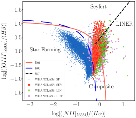
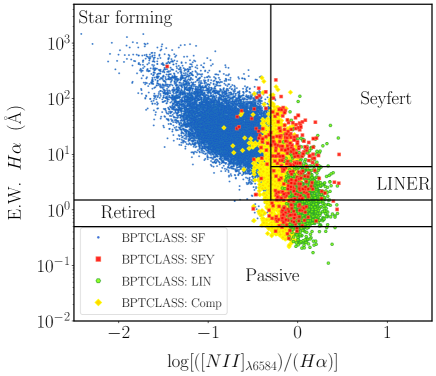
Figure 14: Left: BPT diagram of galaxies grouped according to their WHAN classification (blue=SF, red==SEY, green= LIN, violet=RET). Right: WHAN diagram of galaxies grouped according to their BPT classification (blue=SF, red==SEY, green= LIN, yellow=Comp).

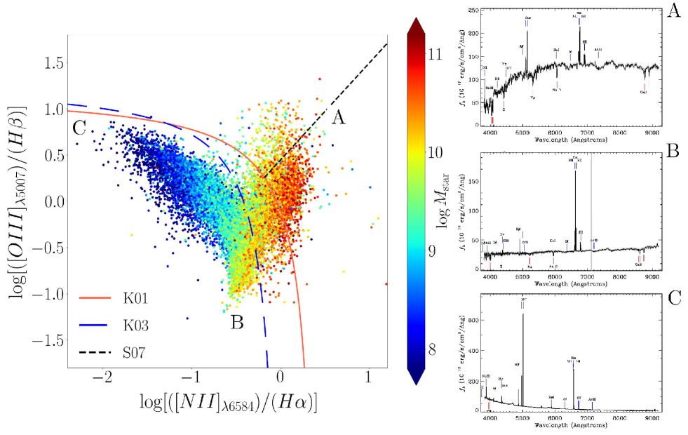
Figure 15: The BPT diagnostic diagrams for galaxies in the SPRING catalogue. Three examples of spectra are given. Colours provide the logarithm of $M_{\mathrm{star}}$ in solar-mass units.

The prominent left wing of the BPT is traced by pure SF nuclei, lying below the empirical line included in the BPT scheme by Kauffmann et al. (2003a) (K03, red straight line in Fig. 13, top panels). Active nuclei (SEY+LIN) are defined as those galaxies which lie on the right wing above the “maximum starburst line” determined by Kewley et al. (2001) (K01, blue long-dashed line). Composite nuclei lie in between AGN and SF nuclei. Seyfert and LINERs are divided by the empirical separation line defined by Schawinski et al. (2007) (S07, black dashed line).

In the top row of Fig. 13, we display the BPT diagnostic diagrams separately for the three chromatic classes (blue cloud, green valley, and red sequence) defined in Sec. $\S$ 2.1.

• In the blue cloud, most galactic nuclei are classified as star-forming ($\sim$90%). Approximately 7% objects are composite, and only few percent are LINERs and Seyfert nuclei ($\sim$2% LIN and $\sim$1% SEY).

• In the green valley, the majority of targets is still found in the SF wing of the BPT, although fewer than in the blue cloud ($\sim$60%). A substantial amount of nuclei falls in the composite and LINERs branches ($\sim$20% and $\sim$16%, respectively). As in the blue cloud, only a small fraction of objects is classified as SEY ($\sim$ 2%).

• Star-forming nuclei in the red sequence decrease to less than a fifth of the total ($\sim$19%), whereas composite and LINERs account for more than half of the RS nuclei ($\sim$38% each). Seyfert nuclei are $\sim$6%.

We point out that our nuclear classification of galaxies belonging to the SPRING sample considers only emission-line galaxies whose nuclear spectra have all four lines with signal-to-noise ratio $>$ 2. This selection introduces a noticeable bias in our classification as far as the RS concerns, since only $\sim$30% of galaxies in the RS (1572 out of 5258) satisfies our criteria, opposite to the BC and the GV, whose majority of galaxies show all four lines in emission, and therefore are classified with the BPT diagram ($\sim$90% and $\sim$70%, respectively).

The mass metallicity relation (cf. Fig. 3 in Thomas et al. 2019) is partly responsible for the pattern in the star-formation arm of the BPT. From $12+\log(\mathrm{O/H})=7.7$ to $12+\log(\mathrm{O/H})=9.2$, most star-forming galaxies with stellar-mass between $10^{8.5}$M_⊙ and $10^{11}$M_⊙ are found, due to the well known correlation between $12+\log(\mathrm{O/H})$ and $\log\mathrm{([NII]/H}\alpha)$ (see, e.g., Yates et al. 2012). However, it does not fully explain the two orders of magnitude decrease in log[OIII]/H$\beta$ over the entire SF branch, a fact that is hinting to a dependence of the ionisation properties on stellar-mass. With increasing stellar-mass, galaxies have decreasing fraction of OB associations in their arms. OB stars are the only stars capable of ionizing Hydrogen and their fraction is a steep function of mass Kennicut-1994; Kennicutt (1998); Boselli et al. (2009). Since OB stars have the shortest lives of all stars this implies that low-mass galaxies have “younger” stellar population than higher mass. This is consistent with the picture of Gavazzi et al. (2002).

3.2 WHAN diagnostic

In addition to the BPT diagnostics, the classification of the nuclear activity based on optical emission-lines is also performed following the two-line WHAN classification scheme. It is a less demanding diagnostic than the BPT, as it only requires the intensities of two lines (H$\alpha$ and [NII]$\lambdaup$6584), and is based on the $\rm[NII]/H\alpha$ ratio combined with the strength of the $\rm H\alpha$ line corrected for underlying stellar absorption. Owing to this two-line diagnostic, even the red-channel spectra such as the majority of those obtained at Loiano Gavazzi et al. (2011, 2013a, 2018) contribute to increasing the number of known AGN, especially those associated with nearby bright galaxies, most affected by the residual incompleteness of the SDSS spectral database.

The WHAN diagnostic was introduced by Cid Fernandes et al. (2010, 2011) to disentangle “true” active nuclei, believed to be triggered by supermassive black holes, from “fake AGN” (retired galaxies), i.e., galaxies with low SFR that are ionised by the hot low-mass evolved stars (HOLMES) within them Trinchieri & di Serego Alighieri (1991); Binette et al. (1994); Macchetto (1996); Cid Fernandes et al. (2004); Stasińska et al. (2008); Sarzi et al. (2010); Capetti & Baldi (2011). We identify five classes of nuclear activity adopting the modified WHAN classification of Gavazzi et al. (2011):

• Star-Forming nuclei (SF): $\log\mathrm{[NII]}/\mathrm{H}\alpha<-0.3$ and EWH$\alpha>1.5$ Å;

• Seyfert (SEY): $\log\mathrm{[NII]}/\mathrm{H}\alpha>-0.3$ and EWH$\alpha>6$ Å;

• LINERs (LIN): $\log\mathrm{[NII]}/\mathrm{H}\alpha>-0.3$ and $6<$ EWH$\alpha$/Å$<1.5$;

• Retired galaxies (RET): EWH$\alpha<1.5$Å;

• Passive galaxies (PAS): EWH$\alpha$, EW[NII] $<0.5$Å.

Table 3: Fractions of the nuclear excitation classes classified with the WHAN diagram (SF, LIN, SEY, RET) calculated in four samples defining the BPT-classified nuclear activity (SF, LIN, SEY, Comp).

	SF (%)	LIN (%)	SEY (%)	RET (%)
SF	99.3	0.1	0.3	0.1
LIN	0.0	34.6	6.3	48.6
SEY	8.9	25.0	40.3	19.7
Comp	16.1	38.3	21.8	17.1

Table 4: Fractions of the nuclear excitation classes classified with the BPT diagram (SF, LIN, SEY, Comp) calculated in four samples defining the WHAN-classified nuclear activity (SF, LIN, SEY, RET).

	SF (%)	LIN (%)	SEY (%)	Comp (%)
SF	93.1	0.0	0.2	2.2
LIN	1.1	26.5	4.8	55.6
SEY	5.6	10.0	15.9	65.7
RET	12.2	40.8	4.1	27.1

Analogously to the BPT, we display the WHAN diagnostic diagrams separately for the three chromatic classes (Fig. 13, bottom panels).

• Star-forming nuclei are the majority of objects in the blue cloud (90%). The fraction of AGN is larger than in the BPT-classification, as both LIN and SEY account for $\sim$4% of the total each. Retired objects are $\sim$1%. Less than 1% of nuclei are passive.

• Approximately 64% nuclei in the green valley are star-forming. LINERs increase to $\sim$20%, whereas the fraction of Seyfert nuclei mildly dereases ($\sim$3%). Retired objects are $\sim$10%. Again, less than 1% of nuclei are passive.

• In the red sequence, star-forming nuclei drop to $\sim$20%. The fraction of LINERs is $\sim$20%. The fractions of retired and passive objects both increase to $\sim$45% and $\sim$16%, respectively. Finally, SEY only account for $\sim 1\%$ of nuclei.

In general, there is a satisfactory agreement between the BPT and the WHAN classification among Star-Forming systems. A visual comparison between the two classification schemes is given in Fig. 14, displaying the BPT (WHAN) diagram of galaxies classified according to the WHAN (BPT).

We observe that the two diagnostics display some noticeable deviations in the classification of non-star-forming nuclei (see Tables 3-4): there are significant overlaps between the classification of Seyfert and LINERs; e.g., most BPT-classified LINERs are identified as Retired by the WHAN diagnostic (48.6%); similarly, most WHAN-classified LINERs are classified as composite nuclei by the BPT (55.6%); the majority of galaxies classified as Seyfert by the BPT are marked the same way by the WHAN (40.3%); conversely, WHAN-classified Seyfert are mostly classified as composite nuclei (65.7%) by the BPT.

The disparity between the BPT and WHAN classifications of AGN (and, especially, LINERs) is not surprising. The two schemes employ a different number of emission-lines, and were proposed following different theoretical and empirical criteria Baldwin et al. (1981); Kewley et al. (2001); Kauffmann et al. (2003a); Cid Fernandes et al. (2011). In addition, there is no clear consensus yet on the ionisation source of LINERs. Heckman (1980) proposed that gas shocks are mainly responsible for LINER-like emission. Halpern & Steiner (1983) and Ferland & Netzer (1983) suggested that the primary mechanism behind the ionisation of LINERs is the accretion of gas onto a central massive black hole. Later, Terlevich & Melnick (1985) and Shields (1992) proposed that the excitation of these nuclei is produced by photoionisation due to hot stars. Recently, Oliveira et al. (2022) argued that a sample of 43 LINERs is probably ionised by post-AGB (asymptotyc giant branch) stars. The uncertainty on the mechanisms driving LINER-like emission could be a major factor for the differences between the BPT and WHAN classifications.

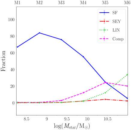
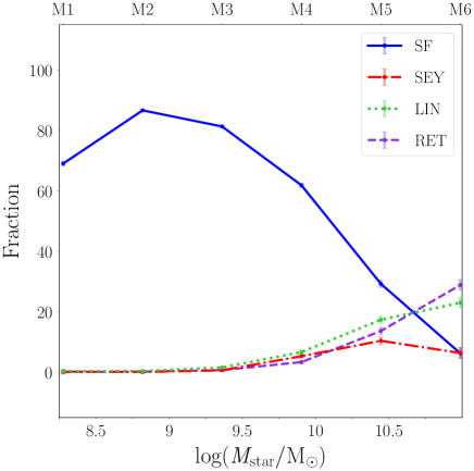
Figure 16: Frequency of BPT (top) and WHAN (bottom) excitation classes as a function of $\log(M_{\mathrm{star}}/\mathrm{M}_{\odot})$ (represented by the six bins M1, … , M6). The binomial errors are computed following Wilson (1927).

3.3 Stellar-mass and environment vs nuclear activity

The ionisation diagnostics considered here are sensitive to the stellar-mass of the targets (see, e.g., Kauffmann et al. 2003a). To explore the relation between nuclear activity and stellar-mass, we classify the galaxy nuclear properties with the BPT and WHAN diagnostics separately in each stellar-mass bin (M1, …, M6). In Fig. 15, we show the BPT diagnostic diagram for the emission-line galaxies in our catalogue. Using different colours to represent different mass bins, we see the characteristic dependence of the nuclear excitation properties on the stellar-mass: in accordance with Kauffmann et al. (2003a), the nuclei of lowest-mass galaxies are SF regions, progressively filling the left-wing of the BPT from top-left to bottom-centre with decreasing ionisation strength (top-bottom) and increasing metallicity (left-right). For three representative regions of the BPT diagram, a typical spectrum is also reported showing the progressive decrease of H$\alpha$ over [NII], and of [OIII] over H$\beta$. Only in the two highest stellar-mass bins (i.e., $10^{10}$ to $\gtrsim 10^{10.5}\ M_{\mathrm{star}}/\mathrm{M}_{\odot}$) a higher fraction of ionised nuclei (LINERs, and, to a lower extent, Seyfert nuclei) is found.

In Fig. 16, we show the incidence of the BPT- and WHAN-classified SPRING emission-line galaxies as a function of their stellar-mass. We see that up to $M_{\mathrm{star}}=10^{9-9.5}\ \mathrm{M}_{\odot}$ (mass bin M3), almost the entire spectroscopic sample is constituted of galaxies with SF nuclei, whose incidence is highest in the M2 bin. The fraction of LINERs becomes non-negligible in the M4 bin ($M_{\mathrm{star}}=10^{9.5-10}\ \mathrm{M}_{\odot}$) and turns out to be dominant over the SF fraction ($\sim 30\%$ over $\sim 10\%$, respectively) for $M_{\mathrm{star}}\gtrsim 10^{10.5}\ \mathrm{M}_{\odot}$ (M6 bin) (see Kauffmann et al. 2003a).

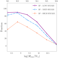
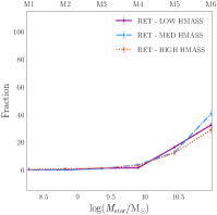
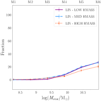
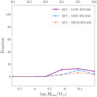
Figure 22: The WHAN-computed frequencies (criteria of Gavazzi et al. (2011)) of star-forming (SF), AGN (SEY), LINER (LIN) and retired (RET) as a function of $\log(M_{\mathrm{star}}/\mathrm{M}_{\odot})$ (represented by the six bins M1, …, M6) in the three halo-mass bins defined in Sec. $\S$ 2.3.2).

To verify if the incidence of the nuclear excitation properties is a general feature of high/low-mass galaxies or, conversely, depends on other environmental features, we replicate Fig. 16 dividing the sample according to $(i)$ the galaxy chromatic class (RS, BC, and GV, Sec. $\S$2.1), $(ii)$ the overdensity parameter (Sec. $\S$2.3.1) and $(iii)$ the halo-mass (Sec. $\S$2.3.2). Our results are reported in Figures 17-22 and summarised in the following:

• (Star-forming): In general, the frequency of SF nuclei is highest in the lower-mass bins M1 - M3 ($M_{\mathrm{star}}\leq 10^{9.5}\ \mathrm{M}_{\odot}$), and decreases as the stellar-mass increases. For a fixed bin of stellar-mass, it diminishes migrating from isolated galaxies to galaxies in clusters, indicating that star-forming systems live in relatively lower-density environments (see also Constantin & Vogeley 2006). A similar decrease is observed as we increase the halo-mass or we move from the blue cloud (BC) to the red sequence (RS). For example, in the M5 bin we find that the BPT-computed SF nuclei are $\sim$45% in the BC, $\sim$10% in the GV, and $\sim$5% in the RS (see Fig. 20, left panel).
  The BPT and WHAN classifications for SF nuclei are in good agreement.

• (LINER): The frequency of LINERs computed with the BPT diagram results little sensitive to the galaxy overdensity and halo-mass (Figs. 18-19 and 21-22). It exhibits the same strong dependence on the stellar-mass in each overdensity and halo-mass bin, as it is consistent with $\sim$0% for $M_{\mathrm{star}}<10^{10}\ \mathrm{M}_{\odot}$, and increases up to $\sim$30%-40% for $M_{\mathrm{star}}>10^{10.5}\ \mathrm{M}_{\odot}$. We find a dependence of the LIN fraction on the chromatic class in the mass range $M_{\mathrm{star}}>10^{10}\ \mathrm{M}_{\odot}$, where it is $\sim$20% higher in the GV than in the BC and RS (Fig. 17, third panel), whereas LIN fractions in the BC and RS are consistent with each other across the whole mass range.
  Conversely, the LIN fraction computed with the WHAN scheme exhibits mild overdensity and halo-mass dependence for $M_{\mathrm{star}}>10^{9.5}\ \mathrm{M}_{\odot}$, increasing by $\sim$5%-10% as galaxies move from high to low overdensity/halo-mass. Consistent with the BPT-computed fraction, we find a similar chromatic dependence of the LIN frequency on the chromatic class in the mass range $M_{\mathrm{star}}>10^{9.5}\ \mathrm{M}_{\odot}$, where galaxies in the GV show a steep increase up to $\sim$50% in the M5 and M6 bins; the fractions of LIN galaxies in the BC and RS are consistent with each other up to $M_{\mathrm{star}}\sim 10^{9.5}\ \mathrm{M}_{\odot}$; in the M5-M6 bins, the LIN fraction in the BC increases to $\sim$30%, whereas the RS fraction settles to less than 10% (Fig. 20, third panel).

• (Seyfert): Unlike the frequency of LINERs, which is found to be increasing with stellar-mass up to 40-50%, the BPT-computed fraction of Seyfert galaxies shows a much milder increase with the stellar-mass and, in general, reaches its maximum ($\sim$5%) in the M5 bin ($10^{10}<M_{\mathrm{star}}/\mathrm{M}_{\odot}<10^{10.5}$). We find a similar dependence of the SEY fraction on the overdensity and halo-mass indicators (i.e., it decreases moving from high to low overdensity/halo-mass, see Figs. 18-19, right panels). Conversely, it does not show considerable dependence on the chromatic class.
  The WHAN-computed SEY fraction displays significant variations with respect to the BPT counterpart. In general, it is consistent with $\sim$0% for $M_{\mathrm{star}}<10^{9.5}\ \mathrm{M}_{\odot}$, and increases for higher masses, reaching a peak in the M5 bin which rises up to $\sim$15% as we move from high to low overdensity/halo-mass galaxies. These results are consistent with Constantin & Vogeley (2006), who observed that Seyfert galaxies reside in less massive halos than those that host LINERs (see Figs. 19 and 22). The fraction of SEY among galaxies in the BC furtherly increases for masses $M_{\mathrm{star}}>10^{10.5}\ \mathrm{M}_{\odot}$ reaching $\sim$18% and $\sim$25% in bins M5 and M6, respectively.

• (Composite): As the LINERs frequency, the frequency of composite (Comp) galaxies reaches its maximum in the highest-stellar-mass bins M5 or M6 and shows a mild dependence on the galaxy overdensity and the halo-mass; i.e., the fraction of composite nuclei in the M4-M6 bins moderately increases migrating from galaxies in clusters (UH) to isolated (UL) galaxies; similarly, the Comp fraction in the higher stellar-mass range is $\sim 5\%$ higher in lower halo-mass galaxies (Fig. 19, second panel). A higher fraction of Comp galaxies is found in galaxies belonging to the GV for all but one (M6) mass bins (Fig. 17, second panel). The Comp frequency in the GV reaches its maximum ($\sim$40%) in the M5 bin.

• (Retired): The fractions of RET in the three overdensity and four halo-mass bins display similar trends, steadily increasing for $M_{\mathrm{star}}>10^{9.5}\ \mathrm{M}_{\odot}$ up to $\sim$30% in the M5 and M6 bins and showing little dependence on the overdensity and the halo-mass; For $10^{9}<M_{\mathrm{star}}\mathrm{M}_{\odot}<10^{9.5}$, it is is few percent higher in the RS than in the BC/GV. For masses $M_{\mathrm{star}}>10^{9.5}\ \mathrm{M}_{\odot}$, it follows similar trends for RS and GV galaxies and is about $\sim$15% lower for galaxies in the BC.

Again, the disparities in the features of non-star-forming nuclei may be attributed to deviations among the BPT and WHAN classifications (Tables 3-4). In general, our results show that one of the most (if not the most) important factor that affects the triggering of nuclear activity is the galaxy stellar-mass Kauffmann et al. (2003a). The dependence of the prevalence of nuclear activity on the local galaxy density and halo-mass appears to indicate that the fraction of Seyfert nuclei decreases towards the highest-density regions and highest halo-masses (see also Sabater et al. 2013, 2015; Li et al. 2019; Lopes et al. 2017), as well as the fraction of star-forming nuclei. The fraction of LINERs displays minor dependencies on the galaxy density and halo-mass, but appears to be related to the galaxy colour in the mass range $M_{\mathrm{star}}>10^{10}\ \mathrm{M}_{\odot}$, where it is $\sim$20% higher in the green valley.

4 Summary

In this work we present the SPRING catalogue, a complete photometric database ($r<17.7$ mag) of local galaxies in the Northern spring sky ($10^{h}<\mathrm{RA}<16^{h}$; $0^{\circ}<\mathrm{Dec}<65^{\circ}$, $cz<10000\ \mathrm{km\ s}^{-1}$) by merging the Portsmouth emission-line table by Thomas et al. (2013) extracted from the SDSS and the NASA-Sloan atlas Blanton et al. (2011). To further reduce the bright-end incompleteness, we complement our sample with the updated Zwicky catalogue (UZC) Zwicky et al. (1961); Falco et al. (1999), and with the UGC catalogue Nilson (1973). We get the available nuclear spectroscopy in the SDSS, and integrate it with optical spectra taken by other surveys Zwicky et al. (1961); Nilson (1973); Ho et al. (1993, 1995, 1997); Falco et al. (1999); Gavazzi et al. (2011, 2013a), and with the spectroscopy obtained by us in 2014-2020 using the Cassini 1.5m telescope of the Loiano Observatory. The SPRING catalogue includes 891 galaxies with optical spectra observed independently from SDSS. We claim that the resulting sample of 30597 targets constitutes the cleanest and most complete catalogue of galaxies available so far for the Northern spring sky limited to $r<17.7$ mag and $cz<10000\ \mathrm{km\ s}^{-1}$. The construction of such a sample constitutes the first goal of the present work (Sec. $\S$ 2).

We study the extensive properties (colours, stellar-mass, H I content) of galaxies in such a sample, confirming that galaxy colour ($\mathrm{NUV}-i$) is a steep function of stellar-mass, with the red sequence well separated from the blue cloud by the green valley (Boselli et al. 2014, Sec. $\S$ 2.1).

We perform a recalibration of the optical diameter-based H I-deficiency parameter employing a reference sample of 3416 isolated galaxies extracted from our catalogue, and find that the slope of the $\log(M(\mathrm{H}\thinspace\scriptsize{\text{I}}))$ vs $\log(D^{2})$ relation is strongly dependent on the galaxy stellar-mass (Sec. $\S$ 2.3.3). We observe that most green-valley objects are consistent with galaxies with deficient H I content, stressing the role of gas in fuelling (and quenching) star-formation, as claimed by Gavazzi et al. (2013c).

Remarkably, we find that a filamentary structure of galaxies extending in the spring sky at intermediate distances between Virgo and Coma contains $\sim$30.7% of H I-deficient galaxies, which significantly exceeds the average H I-deficiency fraction ($\sim$12%) of field galaxies. To probe the relevance of the deficiency of H I in filaments, we construct ten thousand overdensity-matched samples and investigate their H I content. We find that the average fraction of H I-deficient galaxies in the matched-samples is (20.2 $\pm$ 1.6)%. This could point out that galaxies in filaments are more H I-deficient than field galaxies.

The nuclear classification of galaxies in our sample (Sec. $\S$ 3) is based on the four-lines BPT and the two-lines WHAN diagnostic diagrams. We confirm that the fraction of AGN (especially LINERs) over SF nuclei is a steep function of stellar-mass Kauffmann et al. (2003a), i.e., the fraction of AGN (Seyfert and LINERs) is consistent with zero up to $M_{\mathrm{star}}<10^{9.5}$ M_⊙, and becomes $\sim$ 40 % for $M_{\mathrm{star}}>10^{10.5}$ M_⊙. A general agreement between the BPT and WHAN classifications is observed. We investigate the mass-dependency of the excitation properties determined with both diagnostics, and find that star-forming nuclei, Seyfert and LINERs display similar trends (Sec. $\S$ 3.1-3.2).

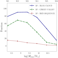
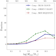
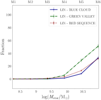
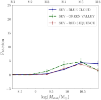
Figure 17: The BPT-computed frequencies of star-forming (SF), AGN (SEY), LINER (LIN) and composite (Comp) as a function of $\log(M_{\mathrm{star}}/\mathrm{M}_{\odot})$ (represented by the six bins M1, …, M6) in the three chromatic regimes (blue cloud, green valley, red sequence, see Sec. $\S$ 2.1). The $y$-axis scale on the right panel (SEY) is magnified to highlight the differences between the three chromatic classes.

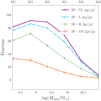
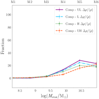
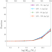
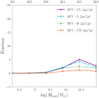
Figure 18: The BPT-computed frequencies of star-forming (SF), AGN (SEY), LINER (LIN) and composite (Comp) as a function of $\log(M_{\mathrm{star}}/\mathrm{M}_{\odot})$ (represented by the six bins M1, …, M6) in the four overdensity bins defined in Sec. $\S$ 2.3.1). The $y$-axis scale on the right panel (SEY) is magnified to highlight the differences between the four overdensity classes.

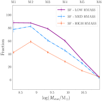
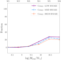
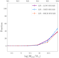
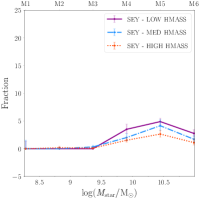
Figure 19: The BPT-computed frequencies of star-forming (SF), AGN (SEY), LINER (LIN) and composite (Comp) as a function of $\log(M_{\mathrm{star}}/\mathrm{M}_{\odot})$ (represented by the six bins M1, …, M6) in the three halo-mass bins defined in Sec. $\S$ 2.3.2). The $y$-axis scale on the right panel (SEY) is magnified to highlight the differences between the three halo-mass classes.

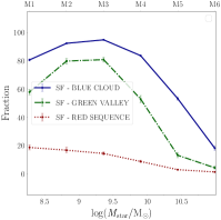
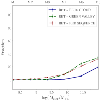
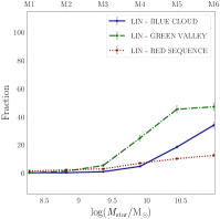
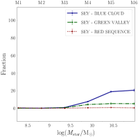
Figure 20: The WHAN-computed frequencies (criteria of Gavazzi et al. (2011)) of star-forming (SF), AGN (SEY), LINER (LIN) and retired (RET) as a function of $\log(M_{\mathrm{star}}/\mathrm{M}_{\odot})$ (represented by the six bins M1, …, M6) in the three chromatic regimes (blue cloud, green valley, red sequence, see Sec. $\S$ 2.1).

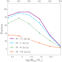
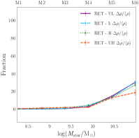
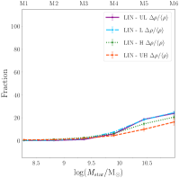
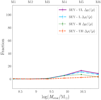
Figure 21: The WHAN-computed frequencies (criteria of Gavazzi et al. (2011)) of star-forming (SF), AGN (SEY), LINER (LIN) and retired (RET) as a function of $\log(M_{\mathrm{star}}/\mathrm{M}_{\odot})$ (represented by the six bins M1, …, M6) in the four overdensity bins defined in Sec. $\S$ 2.3.1).

In addition, we investigate whether the nuclear-excitation fractions depend predominantly on the stellar-mass or on other environmental related indicators (Sec. $\S$ 3.3). To this end, we examine the connection between the mass-dependence of the galaxy excitation properties and their environment, which we determine using three different indicators, i.e., (i) a chromatic criterion, (ii) the local galaxy density, and (iii) the halo-mass of the group to which galaxies belong. In general, we observe that the mass-dependency of the fraction of Seyfert nuclei is little sensitive to the galaxy environment (with noticeable variations in the SEY percentage depending on the adopted diagnostic scheme), while the fraction of star-forming nuclei is a steeper function of stellar-mass in lower-density environments and in blue-cloud galaxies. The fraction of LINERs exhibits a dependence on the galaxy colour and, for $M_{\rm star}\gtrsim 10^{9.5-10}$ M_⊙, is significantly larger in galaxies belonging to the green valley.

5 Discussion

The analysis presented in this work –based on a statistically-significant sample– points out that the main parameter driving the level of nuclear activity is the galaxy stellar-mass Kauffmann et al. (2003a); Decarli et al. (2007); Juneau et al. (2011); Rodríguez del Pino et al. (2017a) and shows that the fraction of AGN does not vary significantly with the galaxy density, the mass of the hosting halo, or the colour of galaxies (see Sec. §3.3). This result overall agrees with the results of Kauffmann et al. (2004) based on a larger SDSS optically-selected sample of galaxies, and with Constantin & Vogeley (2006). They also agree with the results gathered by other teams which analyse optically- and X-rays-selected clusters Vollmer et al. (2001, 2004); Vollmer, B. et al. (2008); Steyrleithner et al. (2020).

Interesting is the fact that the highest density regions in our sample are those within well known clusters of galaxies such as Coma, A1367, and Virgo. Detailed multi-frequency studies of these clusters clearly indicate that the dominant perturbing mechanism affecting the evolution of the infalling, gas-rich spiral population is ram-pressure. This mechanism has been identified without ambiguity by the presence of long cometary tails in H I Gavazzi (1989); Dickey & Gavazzi (1991); Bravo-Alfaro et al. (2001); Scott et al. (2010, 2012); Chung et al. (2007), radio continuum Gavazzi (1978); Gavazzi & Jaffe (1985, 1987); Gavazzi et al. (1995); Miller et al. (2009); Chen et al. (2020); Lal (2020); Vollmer et al. (2004, 2010); Crowl et al. (2005); Kantharia et al. (2008), and H$\alpha$ Yoshida et al. (2002); Boselli et al. (2018); Fossati et al. (2018); Yagi et al. (2007, 2010, 2017), by detailed multifrequency studies of large statistical samples (e.g., Vollmer et al. 2001; Boselli et al. 2014; Gavazzi et al. 2012), and of individual objects Boselli et al. (2016); Kenney & Koopmann (1999); Kenney et al. (2004, 2008); Vollmer (2003); Vollmer et al. (2004); Vollmer, B. et al. (2008).

A relation between the incidence rate of galaxies hosting an AGN and the density of the environment in which they reside has been looked for in several statistical studies, since it is expected in different evolutionary scenarios (e.g., Kauffmann et al. 2004). In a starvation scenario (e.g., Larson et al. 1980), in which the hot halo surrounding galaxies is removed once galaxies become satellites of larger structures, the feedback mechanism induced by a strong nuclear activity easily removes most of the cold-gas component host on the galaxy disc as indicated by the most recent hydrodynamical simulations Stevens et al. (2021); Tonnesen & Bryan (2009); Boselli et al. (2021). For this reason, the activity of star formation of the host galaxies is strongly reduced, producing quiescent systems. Recently, it has also been claimed that the loss of angular momentum which follows a ram-pressure-stripping event might induce gas infall in the galaxy centre, feeding nuclear activity (e.g., Schulz & Struck 2001; Tonnesen & Bryan 2009; Poggianti et al. 2017b; Ramos-Martínez et al. 2018).

Our analysis of the nuclear properties of galaxies in different environments and stellar-mass ranges shows that the incidence of Seyfert nuclei in galaxies within the core of a cluster (UH overdensity) is minimum (Figs. 18-21). This result agrees with a number of recent works aimed at studying the incidence of strong AGN in different environments Sabater et al. (2013, 2015); Li et al. (2019); Lopes et al. (2017). Conversely, the incidence of nuclei with BPT-classified LINER-like emission-line ratios displays no dependence on the local galaxy overdensity (Fig. 18, third panel), but is strongly connected with the galaxy stellar-mass and reaches $\sim 40\%$ for $M_{\mathrm{star}}>10^{10.5}\ \mathrm{M}_{\odot}$ (similar results yield for LINERs classified by the WHAN diagnostic). This evidence is at odds with the results of Poggianti et al. (2017b), who found an enhanced AGN (Seyfert) fraction in a sample of ram-pressure-stripped (jellyfish) objects (5/7). However, such results were not confirmed by the follow-up analysis of Peluso et al. (2022) on a larger selection of jellyfish galaxies. The recent analysis by Roman-Oliveira et al. (2019) of a sample of ram-pressure-stripped galaxies did not find a high incidence of AGN (5/70). The disparities between these studies may be attributed to the different nuclear-activity classification schemes which they adopt. Poggianti et al. (2017b) and Peluso et al. (2022) use the BPT diagnostic, while the classification of the sample analysed in Roman-Oliveira et al. (2019) employs the WHAN (see also Rodríguez del Pino et al. (2017b)). As we point out in Sec. §3.2, the two diagrams display noticeable deviations in the classification of non-star-forming nuclei (e.g., among the galaxies classified as Seyfert by the BPT, only $\sim 16\%$ are classified as SEY by the WHAN).

Another potential element of discrepancy among different analyses of the nuclear activity vs environment relation is the characterization of AGN. Poggianti et al. (2017b) denotes as AGN those galaxies which are classified as Seyfert by the BPT diagram; Peluso et al. (2022) classifies a galaxy as an AGN if its nuclear region has a Seyfert or LINER BPT-classification; similarly, Rodríguez del Pino et al. (2017b) labels as AGN those galaxies which are classified as Seyfert or LINERs by the WHAN. As we see in Figs. 17-19, active nuclei classified with the BPT diagnostic diagram are dominated by the LINERs, suggesting that more lenient AGN definitions are biased toward LINER-like behavior. LINERs differ from Seyferts in many of their characteristics; also, the ionisation source of LINER-like objects is still uncertain. Thus, caution should be exercised when investigating the interplay between the galaxy environmental properties (e.g., being subject to ram-pressure-stripping) and the triggering of nuclear activity.

As extensively discussed in Boselli et al. (2022), the results of Poggianti et al. (2017b) may be due to the fact that their sample of 7 galaxies was composed of very massive objects ($M_{\mathrm{star}}>4\times 10^{10}\ \mathrm{M}_{\odot}$) which are more likely to host an active nucleus. The sample examined by Poggianti et al. (2017b) has been further expanded in Peluso et al. (2022), who considered a total of 51 galaxies observed in the context of the GASP survey Poggianti et al. (2017a) along with additional 82 galaxies retrieved from the literature and found that the fraction of galaxies which host a AGN (Seyfert or LINER) is $\sim 27\%$ at masses $M_{\mathrm{star}}>10^{9}\ \mathrm{M}_{\odot}$, and $\sim 51\%$ at masses $M_{\mathrm{star}}>10^{10}\ \mathrm{M}_{\odot}$. The majority of objects considered by Peluso et al. (2022) are high-mass galaxies (all galaxies hosting a AGN in GASP have $M_{\mathrm{star}}>10^{10.5}\ \mathrm{M}_{\odot}$). In contrast to Poggianti et al. (2017b), the AGN fractions considered by Peluso et al. (2022) include both Seyfert and LINERs. Also, the AGN fractions are calculated with respect to a sample of emission-line galaxies only, introducing possible bias. For comparison, the BPT-computed SEY+LIN fraction $f_{\mathrm{(SEY+LIN)}}/f_{\mathrm{ELG}}$ of SPRING galaxies in the M6 bin (i.e., with stellar-mass $M_{\mathrm{star}}>10^{10.5}\ \mathrm{M}_{\odot}$) calculated over all emission-line galaxies in the same stellar-mass bin is $\sim 58.2\%$, whereas the fraction $f_{\mathrm{(SEY+LIN)}}/f_{\mathrm{TOT}}$ in the same mass range (where $f_{\mathrm{TOT}}$ accounts for both emission-line and passive galaxies) is $\sim 37\%$. In general, our analysis suggests that the investigation of the occurrence of AGN in different galaxy environments requires care, as one needs to take into account possible biases that may arise due to (i) the particular diagnostic adopted (BPT vs WHAN vs other diagnostics), (ii) the characterization of AGN (are LINERs true AGN?), and (iii) the sample which defines the underlying galaxy population.

Finally, our analysis suggests that the incidence of LINERs is higher in galaxies belonging to the green-valley (Figs. 17 and 20). In a future companion paper, we aim to further investigate the nuclear activity vs environment relation of a sample of SPRING galaxies which are subject to ram-pressure-stripping in the cluster environment.

Appendix A Loiano observations

We used the Bologna Faint Object Spectrograph and Camera (BFOSC, Gualandi & Merighi 2001) attached to the 152cm F/8 Cassini Telescope locatedin Loiano, which belongs to the Observatory of Bologna, to obtain optical spectra of the nuclei of 376 galaxies. The observations took place from 2014 to 2020. The long-slit spectra were taken through a slit of 2 or 2.5 arcsec width (depending on the seeing conditions), with a intermediate-resolution red-channel grism (R $\sim$ 2200) that covers the 6100 - 8200 Å portion of the spectrum, which contains H$\alpha$, [NII], and [SII] lines (three galaxies were observed also using a blue-channel grism covering H$\beta$ and [OIII]).

The detector used by BFOSC is an EEV LN/1300-EB/1 CCD of 1300x1340 pixels, with 90% quantum efficiency near 5500 Å. Its spatial scale of 0.58 arcsec/pixel results in a field of view of $12.6^{\prime}\times 13^{\prime}$. The dispersion of the red-channel grism is 8.8 nm/mm and results in spectra with 1.6  Å/pix. The instrumental broadening is typically 6 Å full-width-half-maximum (FWHM), as checked on the 6300.3 Å sky line. We obtained exposures of 3-5 minutes, repeated typically three-six times per run (to remove the cosmic rays), but several galaxies were re-observed in more than one run (see Table LABEL:data2). The seeing at Loiano is typically 1.5 - 2.5 arcsec. The slit was mostly set in the E-W direction, except when it was positioned along the galaxy major axis or along the direction connecting two adjacent objects to accommodate both in one exposure.

The wavelength was calibrated using frequent exposures of a He-Ar hollow-cathode lamp. We used several sky lines to check a posteriori the wavelength calibration. The spectrograph response was obtained by daily exposures of the star Feige-34.

Table LABEL:data2 summarises the spectra obtained at Loiano (2014-2020) as follows:

1. Column 1: Galaxy name;
   

2. Column 2,3: Right Ascension; Declination (J2000);
   

3. Column 4: redshift $cz$ (km/s);
   

4. Column 5: $r$-band magnitude;
   

5. Column 6: duration of the individual exposures;
   

6. Column 7: number of individual exposures;
   

7. Column 8: observing date;
   

8. Column 9: slit orientation (counterclockwise from N) 270 corresponds to East-West;
   

9. Column 10: measured EW of the H$\alpha$ line (negative EW values represent emission);
   

10. Column 11: measured EW of [NII]$\mathrm{\lambdaup}\ 6584$ line;
    

11. Column 12: measured EW of H$\beta$ line;
    

12. Column 13: measured EW of [OIII]$\mathrm{\lambdaup}\ 5007$ line.

Table 5: List of 302 galaxies whose spectra have been taken at Loiano between 2014 and 2020.

ID	RA	DEC	$cz$	$r$	Tint	N	Obs date	PA slit	EW $H\alpha$	EW NII	EW $H\beta$	EW [OIII]
	Deg	Deg	$\rm kms^{-1}$	mag	sec		Y-M-D	Deg	Å	Å	Å	Å
(1)	(2)	(3)	(4)	(5)	(6)	(7)	(8)	(9)	(10)	(11)	(12)	(13)
J073637+3175303	114.15417	17.88417	5037	11.65	300	3	2014-02-27	270	0	-0.97	-	-
CGCG 119-029	124.35751	21.68547	3566	13.55	600	3	2014-02-27	290	-20.59	-7.62	-	-
CGCG 119-057	124.95133	22.03145	3584	13.55	600	3	2014-02-27	345	0	-1.18	-	-
NGC-3065	150.47922	72.17047	2000	-	300	3	2014-03-27	336	0	-2.16	-	-
NGC-3066	150.54463	72.12587	2049	-	300	3	2014-03-27	336	-29.33	-12.84	-	-
NGC-3094	150.35809	15.77007	2404	14.41	300	3	2014-03-29	270	-20.79	-16.15	-	-
NGC-3098	150.56956	24.71110	1387	12.04	300	3	2014-02-27	268	-0.39	0	-	-
NGC-3119S	151.71613	14.37298	8825	12.47	300	3	2014-02-27	209	0	0	-	-
NGC-3119N	151.71738	14.37540	9090	16.64	300	3	2014-02-27	209	0.36	-1.19	-	-
MRK-26	152.96463	58.88997	9122	15.43	420	3	2014-02-27	330	-76.22	-13.84	-	-
UGC-5491	152.99252	58.86464	9100	14.48	420	3	2014-02-27	270	0	0	-	-
NGC-3163	153.52959	38.65255	6258	13.00	300	3	2014-03-28	270	0	-1.72	-	-
J101408+383908.6	153.53553	38.65239	6190	15.79	300	3	2014-03-28	270	0	0	-	-
NGC-3222	155.64379	19.88703	5585	12.62	180	3	2014-02-27	270	0	0	-	-
LSBCF-568-09	157.05006	18.60652	8062	14.20	300	3	2014-03-29	270	-14.60	-6.70	-	-
NGC-3303NED02	159.25038	18.13590	6176	12.42	300	3	2014-03-28	270	-9.46	-17.33	-	-
MRK-723	159.42479	23.67333	5456	14.96	300	3	2014-03-29	195	-45.05	-10.75	-	-
UGC-5798	159.94508	47.93169	1517	14.41	600	3	2014-03-28	225	-64.91	-6.57	-	-
CGCG-155-021NED02	162.29193	29.81590	9465	13.86	600	5	2014-03-29	195	0	-2.14	-	-
NGC-3419N	162.82608	13.94722	3035	13.35	300	3	2014-03-28	244	0.38	-1.06	-	-
NGC-3419S	162.82393	13.94599	3035	13.86	300	3	2014-03-28	244	2.75	-2.75	-	-
NGC-3415	162.92748	43.71262	3303	12.11	600	3	2014-03-28	270	0	-1.84	-	-
ARK-271	164.69537	59.48680	6935	15.73	300	3	2014-03-28	272	-37.64	-7.09	-	-
UGC-6073NED01	164.93826	17.65014	8813	14.77	600	3	2014-03-28	240	-9.66	-6.27	-	-
UGC-6073NED02	164.94362	17.65314	8813	14.83	600	3	2014-03-28	240	-20.75	-7.36	-	-
UGC-6106	165.54664	45.88900	6552	13.44	600	4	2014-03-29	336	-10.07	-7.57	-	-
UGC-6127	166.01419	49.82160	7186	14.80	420	3	2014-05-28	270	-11.97	-4.32	-	-
UGC-6173	166.83094	23.48373	6599	13.74	600	3	2014-03-29	336	-40.97	-22.06	-	-
MRK-0423-N	171.70211	35.25086	9674	14.17	300	3	2014-03-29	270	-81.70	-37.05	-	-
MRK-0423-S	171.70272	35.24803	9674	15.48	300	3	2014-03-29	270	-9.38	-17.16	-	-
NGC-3682	171.92165	66.58984	1515	11.93	300	3	2014-05-28	272	-5.45	-3.42	-	-
NGC-3683	172.299 0	57.13233	2427	12.58	300	4	2014-05-28	260	-1.50	-1.40	-	-
UGC-6527NED3	173.14710	52.94710	8346	15.73	300	2	2014-03-29	253	-21.09	-16.07	-	-
UGC-6527NED2	173.15293	52.94767	8110	14.38	300	2	2014-03-29	253	0	0	-	-
UGC-6527NED1	173.16732	52.95000	7919	14.12	300	3	2014-03-29	253	-47.30	-20.30	-	-
NGC-3762	174.34931	61.75936	3463	12.51	300	1	2014-05-28	270	0	0	-	-
NGC-3822	175.54629	10.27779	6267	12.73	300	3	2014-03-29	351	-21.18	-23.64	-	-
CGCG-97-092	177.00042	20.19003	6487	14.93	300	3	2014-03-29	351	-74.13	-23.47	-	-
NGC-3894	177.20983	59.41566	3223	11.45	300	2	2014-05-29	270	-1.32	-5.54	-	-
NGC-3990	179.39816	55.45867	696	12.31	300	3	2014-03-29	275	-4.96	-5.86	-	-
NGC-3998	179.48388	55.45350	1048	11.47	300	3	2014-03-29	275	0	0.	-	-
NGC-4085	181.34463	50.35295	746	12.48	600	4	2014-03-30	257	-43.46	-14.88	-	-
NGC-4278	185.02843	29.28075	620	10.28	300	3	2014-03-29	239	-5.21	-7.48	-	-
NGC-4283	185.08686	29.31094	984	12.04	300	3	2014-03-29	239	0	0.	-	-
NGC-4301	185.61337	04.56628	1273	13.40	300	4	2014-05-31	287	-24.48	-3.29	-	-
NGC-4474	187.47311	14.06859	1588	11.35	300	3	2014-02-28	270	0	0.	-	-
NGC-4528	188.52531	11.32126	1342	11.98	300	3	2014-05-29	270	0	0.	-	-
NGC-4550	188.87742	12.22082	459	11.47	180	3	2014-03-29	270	0	-1.50	-	-
NGC-4551	188.90814	12.26398	1172	11.55	180	3	2014-03-29	215	0	0.	-	-
UGC-7905NED01	190.94974	54.89597	4933	14.10	300	3	2014-03-29	201	-65.71	-12.76	-	-
UGC-7905NED02	190.95591	54.90495	4875	15.16	300	3	2014-03-29	201	-103	-10.87	-	-
NGC-4774NED02	193.27735	36.81983	8341	14.57	300	3	2014-02-28	346	-137.0	-46.88	-	-
NGC-4774NED01	193.27513	36.82632	8373	16.58	300	3	2014-02-28	346	-39.58	-15.33	-	-
NGC-4774NED03	193.27742	36.81887	8374	14.50	300	3	2014-02-28	346	-80.5	-27.15	-	-
NGC-4861	194.75975	34.85944	835	13.71	300	3	2014-02-28	204	-660.7	-12.93	-	-
NGC-4868	194.78708	37.31033	4665	12.03	300	3	2014-02-28	270	-19.13	-8.36	-	-
UGC-8451	201.72473	32.19320	5275	13.44	180	5	2014-04-29	270	0	0.	-	-
NGC-5243	204.06229	38.34392	4205	13.16	300	3	2014-04-29	270	-12.96	-5.76	-	-
NGC-5278	205.41508	55.67065	7541	13.40	300	3	2014-03-29	252	-12.68	-15.51	-	-
NGC-5279	205.43229	55.67381	7580	14.17	300	3	2014-03-29	252	-14.44	-12.78	-	-
NGC-5351	208.36547	37.91497	3610	12.12	420	3	2014-05-29	278	-4.90	-3.72	-	-
NGC-5389	209.02636	59.74204	1842	11.70	300	3	2014-04-29	270	0.60	-1.35	-	-
NGC-5380	209.23620	37.61038	3173	12.51	300	3	2014-05-31	270	0	0.	-	-
NGC-5394	209.64022	37.45349	3448	13.36	300	3	2014-05-31	270	-46.74	-27.87	-	-
NGC-5422	210.17516	55.16448	1820	11.92	300	3	2014-04-30	270	0.18	-1.69	-	-
NGC-5440	210.75434	34.75787	3689	11.91	300	3	2014-05-29	270	-1.71	-5.45	-	-
NGC-5480	211.58971	50.72486	1856	12.37	300	3	2014-05-31	273	-44.71	-15.7	-	-
NGC-5481	211.67197	50.72333	2132	12.37	300	3	2014-05-31	273	0	-0.65	-	-
IC-983	212.51822	17.73385	5443	13.16	300	3	2014-05-28	279	0	0.	-	-
UGC-9098NED01	213.11052	45.69041	8406	14.40	600	3	2014-03-30	266	-31.39	-15.08	-	-
UGC-9098NED02	213.122375	45.69097	8156	14.30	600	3	2014-03-30	266	-46.19	-15.22	-	-
NGC-5533	214.03226	35.34383	3866	11.77	300	3	2014-04-30	270	-1.70	-4.44	-	-
NGC-5614	216.03162	34.85885	3892	11.73	300	3	2014-05-28	271	-0.79	-3.77	-	-
NGC-5752	221.309 0	38.72885	4539	14.58	300	3	2014-03-30	262	-86.32	-30.16	-	-
NGC-5754	221.33186	38.73121	4561	12.99	300	3	2014-03-30	262	0	0.	-	-
NGC-5784	223.56854	42.55791	5370	12.31	300	3	2014-05-29	270	0	-2.14	-	-
NGC-5820	224.66592	53.88608	3335	11.96	300	3	2014-05-31	270	0	0.	-	-
NGC-5839	226.36454	1.634810	1225	12.34	300	3	2014-02-28	270	0	0.	-	-
NGC-5845	226.50338	1.633800	1450	12.25	300	3	2014-02-28	270	0	0.	-	-
UGC-9794	229.04528	10.50965	6464	13.03	420	3	2014-05-30	206	-2.68	-4.59	-	-
NGC-5908	229.18008	55.40925	3306	12.04	300	3	2014-04-30	270	-1.18	-2.16	-	-
NGC-5953	233.63492	15.19377	1965	12.08	300	3	2014-03-30	239	-19.59	-24.45	-	-
NGC-5954	233.64592	15.20006	1959	13.21	300	3	2014-03-30	239	-79.27	-31.21	-	-
NGC-5981	234.47271	59.39175	1764	13.14	300	3	2014-04-30	270	-2.02	-2.06	-	-
NGC-5987	234.98904	58.07953	3010	11.77	180	3	2014-02-28	244	0	0.	-	-
CGCG-166-030	235.14696	28.36066	9805	13.68	300	3	2014-05-31	270	0	0.	-	-
NGC-5992	236.08963	41.08636	9518	14.01	300	3	2014-03-30	209	-51.73	-18.41	-	-
NGC-5993	236.11508	41.12081	9565	13.81	300	3	2014-03-30	209	-34.42	-23.68	-	-
UGC-10070	237.80363	47.25490	5958	12.99	300	3	2014-05-30	289	-3.73	-5.72	-	-
NGC-6012	238.55808	14.60125	1854	12.42	300	5	2014-03-30	331	-2.5	-2.90	-	-
UGC-10097	238.93023	47.86728	5962	12.30	300	3	2014-05-30	270	-0.39	-2.89	-	-
NGC-6014	238.98917	5.931890	2491	12.67	300	3	2014-06-01	270	-56.49	-27.27	-	-
NGC-6018	239.37406	15.87262	5218	13.46	300	3	2014-04-30	270	-4.72	-4.94	-	-
NGC-6027b	239.79514	20.76219	4053	14.84	420	3	2014-06-01	286	0	0.	-	-
J10001207+0938549	150.05021	9.648730	5411	13.91	300	3	2015-04-13	270	-1.78	-3.58	-	-
UGC-5501	153.04896	4.923390	8517	13.99	300	3	2015-04-13	270	-16.10	-7.38	-	-
CGCG-037-092	159.14919	5.910580	3505	13.82	240	3	2015-03-23	270	-26.03	-17.05	-	-
NGC-3405NED01	162.43045	16.23883	6439	13.53	300	3	2015-04-13	270	0	0	-	-
UGC-5928	162.44644	51.89419	7393	13.46	300	3	2015-04-14	270	0	0	-	-
NGC-3388	162.85636	8.567150	6627	13.22	300	3	2015-04-13	270	0	0	-	-
UGC-6003	163.26601	4.631850	5819	14.00	300	4	2015-04-13	270	-77.92	-24.00	-	-
UGC-6117	165.79055	50.20620	7262	13.53	300	3	2015-04-14	270	-2.86	-6.61	-	-
UGC-6175NED01	166.83146	18.42989	8231	14.39	300	3	2015-04-13	270	0	-1.90	-	-
UGC-6175NED02	166.83692	18.43291	7959	14.42	300	3	2015-04-13	270	-5.00	-2.90	-	-
NGC-3599	168.86231	18.11039	839	12.07	180	5	2015-05-20	270	-0.93	-3.19	-	-
UGC-6361NED01	170.19406	0.470610	7237	13.94	300	3	2015-04-15	270	0	-2.79	-	-
UGC-6361NED02	170.20006	0.468579	7295	13.99	300	3	2015-04-15	270	0	0	-	-
NGC-3641	170.28673	3.194590	1755	13.20	300	3	2015-04-15	270	0	0	-	-
NGC-3658	170.99277	38.56234	2045	12.14	300	3	2015-04-14	270	0	0	-	-
NGC-3697	172.20990	20.79501	6261	12.97	300	3	2015-04-15	270	-0.86	-2.34	-	-
NGC-3712	172.78814	28.56794	1580	12.58	420	3	2015-04-15	270	-30.40	-4.49	-	-
UGC-6545	173.43358	32.63364	2619	13.46	300	3	2015-04-15	270	-2.00	-3.29	-	-
NGC-3764NED01	174.22759	17.88860	3432	13.91	300	3	2015-04-13	270	0	0	-	-
NGC-3767	174.31482	16.87717	6362	13.12	300	3	2015-04-13	270	-0.55	-1.90	-	-
NGC-4008	179.57100	28.19250	3620	11.73	300	3	2015-04-14	270	0	0	-	-
IC-3014	182.15417	38.83177	6333	13.62	300	3	2015-04-14	270	-19.45	-13.44	-	-
IC-3014-HII	182.15556	38.83871	6333	16.59	300	3	2015-04-14	270	-123.7	-40.07	-	-
NGC-4227	184.14040	33.52207	6450	12.47	300	3	2015-04-15	270	0	-1.51	-	-
NGC-4296	185.36829	6.653560	4099	12.69	300	3	2015-04-15	270	0	0	-	-
NGC-4377	186.30128	14.76221	1338	11.69	240	3	2015-05-20	270	0	0	-	-
NGC-4410E	186.62290	9.019030	7566	13.06	300	3	2015-04-14	270	0	-2.45	-	-
NGC-4410W	186.61784	9.019970	7218	13.22	300	3	2015-04-14	270	-22.64	-13.38	-	-
NGC-4434	186.90285	8.154340	1071	11.85	300	3	2015-04-14	270	-13.41	-3.93	-	-
NGC-4458	187.23985	13.24189	635	11.92	300	3	2015-04-15	270	0	0	-	-
NGC-4544	188.90239	3.034530	1154	13.00	300	3	2015-04-14	270	-13.80	-4.21	-	-
IC-3617	189.85417	7.965830	2075	14.37	420	3	2015-04-15	270	-47.08	-4.71	-	-
NGC-5100NED02	200.24829	8.978310	9576	13.50	300	3	2015-05-20	270	-22.17	-14.22	-	-
UGC-8471	202.21713	38.57769	7943	13.61	300	3	2015-04-16	270	-5.57	-3.14	-	-
NGC-5223	203.60508	34.69043	7205	12.14	300	4	2015-04-14	270	0	0	-	-
NGC-5331NED01	208.06729	2.100917	9833	14.12	300	3	2015-04-16	270	-37.7	-15.37	-	-
NGC-5331NED02	208.06843	2.108630	9910	14.06	300	3	2015-04-16	270	-17.95	-9.98	-	-
NGC-5386	209.59307	6.339100	4289	13.39	300	3	2015-05-20	270	-3.93	-4.79	-	-
NGC-5611	216.01990	33.04739	1968	12.45	240	3	2015-05-20	270	0	0	-	-
UGC-9241	216.33580	32.48237	4175	13.91	300	3	2015-05-20	270	-22.19	-7.59	-	-
NGC-5639	217.19396	30.41294	3553	13.45	300	3	2015-05-21	270	-4.60	-2.38	-	-
NGC-5674	218.46768	5.458240	7474	13.22	300	3	2015-04-15	270	-21.65	-18.89	-	-
UGC-9412	219.09195	58.79427	9430	13.68	300	4	2015-04-15	270	-235	-85	-	-
UGC-9454	220.09933	6.307200	7148	14.06	300	5	2015-04-16	270	-2.87	-2.17	-	-
NGC-5770	223.31257	3.959730	1491	12.02	240	3	2015-05-20	270	0	0	-	-
UGC-9622	224.33885	19.67294	4838	13.43	300	3	2015-04-16	270	-14.75	-6.97	-	-
NGC-5854	226.94874	2.568640	1737	11.82	240	3	2015-05-20	270	0	0	-	-
NGC-5864	227.38983	3.052750	1885	14.40	240	3	2015-05-20	270	0	0	-	-
NGC-5869	227.45605	00.46996	2085	11.70	240	3	2015-05-20	270	0	0	-	-
NGC-5869E	227.47467	00.46980	27116	-	240	3	2015-05-20	270	0	0	-	-
UGC-9755	227.80470	10.45145	9024	13.81	300	3	2015-04-16	270	0	0	-	-
NGC-5926	230.85375	12.71528	6189	14.00	300	3	2015-04-14	270	-37.47	-17.26	-	-
NGC-5954	233.64656	15.19824	1959	13.21	300	3	2015-04-15	270	-13.99	-5.78	-	-
CGCG-166-011	233.81141	27.32497	9631	13.68	240	3	2015-05-21	270	0	0	-	-
NGC-5987	234.98909	58.07954	3010	11.77	300	3	2015-04-15	270	0	0	-	-
IC-4569	235.20156	28.29209	9821	13.56	240	3	2015-05-21	270	0	0	-	-
IC-4572	235.47580	28.13401	9959	13.43	240	3	2015-05-21	270	-2.9	-8.09	-	-
J154427.40+410718.4	236.11418	41.12180	9687	14.91	300	3	2015-05-21	270	-30.00	17.76	-	-
CGCG-166-064	237.64212	28.63852	9612	14.28	240	4	2015-05-21	270	0	0	-	-
UGC-10074	238.19940	24.39021	9613	14.33	300	3	2015-04-15	270	-4.70	-2.23	-	-
NGC-6010	238.57980	0.543050	1889	12.12	300	3	2015-04-16	270	0	-0.69	-	-
NGC-2444	116.721060	39.03197	4048	13.14	600	3	2016-02-11	270	0	0	-	-
NGC-2445	116.729592	39.01512	4002	13.51	600	3	2016-02-11	270	-52.00	23.90	-	.-
NGC-2481	119.307183	23.76769	2157	12.37	300	3	2016-02-11	270	0	-0.60	-	-
NGC-2577	125.681041	22.55309	2062	11.91	300	3	2016-02-11	270	0	0	-	-
NGC-2592	126.783547	25.97031	1979	12.12	300	3	2016-02-13	270	0	-0.33	-	-
NGC-2594	126.821501	25.87880	2362	13.27	300	3	2016-02-13	270	0	0	-	-
NGC-2764	137.072924	21.44333	2706	12.53	420	3	2016-02-13	200	-38.40	-17.66	-	.-
NGC-2778	138.101560	35.02753	2049	12.25	300	3	2016-02-13	270	0	0	-	-
NGC-2962	145.224716	05.16584	1967	11.89	420	1	2016-02-13	270	0	-2.38	-	-
NGC-3032	148.033953	29.23622	1562	12.34	300	1	2016-02-13	270	-9.00 .	-5.49	-	.-
NGC-3248	156.939160	22.84694	1481	12.22	300	3	2016-03-07	270	0	0	-	-
NGC-3605	169.194170	18.01694	661	12.57	300	3	2016-03-07	270	0	0	-	-
NGC-3630	170.070830	2.964444	1499	11.83	300	3	2016-03-07	270	0	0	-	-
NGC-4078	181.198750	10.59583	2546	12.75	420	3	2016-03-07	270	0	0	-	-
UGC-3596	103.898775	39.76462	5049	12.49	360	3	2017-02-22	270	0	-1.40	-	-
NGC-2388	112.222720	33.81904	4134	13.12	300	3	2017-02-21	270	-20.39	-7.53	-	-
UGC-3876	112.322886	27.90048	854	13.17	480	3	2017-02-25	360	0	0	-	-
NGC-2411	113.651475	18.28151	5073	12.86	300	3	2017-02-25	270	0	0	-	-
UGC-3995	116.038040	29.24744	4750	12.56	300	4	2017-02-22	286	-5.45	-8.49	-	-
NGC-2435	116.056601	31.65113	4189	12.59	300	3	2017-03-23	270	0	0	-	-
NGC-2445	116.729592	39.01512	4002	13.51	300	3	2017-02-21	270	-42.15	-20.86	-	-
NGC-2476	119.188277	39.92787	3729	12.42	300	4	2017-03-23	270	0	0	-	-
NGC-2485	119.188590	7.479154	9826	15.30	300	3	2017-02-21	270	-25.46	-15.79	-	-
NGC-2485	119.202072	7.478494	4610	12.45	300	3	2017-02-21	270	-4.44	-5.94	-	-
NGC-2481	119.307183	23.76769	2157	12.37	300	3	2017-02-22	276	0	-1.14	-	-
NGC-2496N	119.655620	08.02966	9562	12.52	300	3	2017-04-20	357	0	0	-	-
NGC-2496S	119.655847	08.02785	9562	12.52	300	3	2017-04-20	357	0	0	-	-
NGC-2493	120.098617	39.83040	3910	11.86	300	3	2017-03-30	270	0	-1.93	-	-
NGC-2507	120.405183	15.70987	4563	11.95	300	3	2017-02-25	270	0	0	-	-
NGC-2513	120.602730	09.41359	4665	11.51	300	3	2017-03-30	270	0	0	-	-
UGC-4203	121.024424	05.11383	4046	13.32	400	3	2017-02-21	270	-167.00	-23.20	-	-
UGC-4228	121.699754	05.30944	4481	12.54	300	3	2017-03-30	270	0	0	-	-
NGC-2532	122.563325	33.95649	5252	12.98	420	3	2017-02-21	270	-6.63	-4.20	-	-
NGC-2554	124.472817	23.47210	4158	11.72	300	3	2017-02-22	270	-1.08	-2.87	-	-
NGC-2577	125.681041	22.55309	2062	11.91	300	3	2017-04-22	270	0	0	-	-
NGC-2592	126.783547	25.97031	1979	12.12	300	3	2017-04-22	270	0	-0.63	-	-
NGC-2661	131.498130	12.61992	4108	14.43	420	3	2017-02-25	270	-32.50	-10.10	-	-
NGC-2672	132.341233	19.07496	4343	11.51	300	3	2017-04-21	270	0	0	-	-
NGC-2672E	132.350660	19.07397	3758	13.26	300	3	2017-04-21	270	0	0	-	-
NGC-2720	134.783708	11.14908	8895	12.64	300	3	2017-04-08	270	0	0	-	-
NGC-2749	136.338804	18.31312	4190	11.89	300	3	2017-04-08	270	-0.89	-2.50	-	-
NGC-2764	137.072924	21.44333	2706	12.53	300	3	2017-04-08	270	-36.80	-18.7	-	-
NGC-2778	138.101560	35.02753	2049	12.25	300	3	2017-04-08	270	0	-0.73	-	-
NGC-2894	142.376037	07.71881	2146	12.42	300	3	2017-04-19	270	0	-0.91	-	-
NGC-2906	143.026029	08.44190	2140	12.36	300	3	2017-04-19	270	0	-1.71	-	-
NGC-2962	145.224716	05.16583	1967	11.89	300	3	2017-04-19	270	0	-1.62	-	-
NGC-2955	145.319242	35.88226	7013	12.60	300	3	2017-02-25	335	-8.30	-3.80	-	-
NGC-2964	145.726046	31.84721	1328	11.46	300	3	2017-02-22	277	-33.50	-16.80	-	-
NGC-2990	146.571746	05.70884	3088	12.81	300	3	2017-02-25	270	-31.70	-10.90	-	-
NGC-2991	146.708800	22.01401	7455	12.84	300	3	2017-04-19	270	0	-0.49	-	-
NGC-3003	147.150208	33.42148	1478	12.42	300	3	2017-02-22	256	-67.90	-23.8	-	-
NGC-3032	148.033953	29.23622	1562	12.34	300	3	2017-02-25	270	-8.10	-4.90	-	-
NGC-3130	152.051420	9.976990	8191	13.63	300	3	2017-02-22	270	0	0	-	-
NGC-3226	155.862530	19.89852	1315	11.28	300	3	2017-02-21	336	-1.14	-2.85	-	-
NGC-3227	155.877410	19.86505	1157	12.27	300	3	2017-02-21	270	-5.36	-10.99	-	-
UGC-5947	162.626250	19.64500	1251	18.12	600	3	2017-02-25	205	0	0	-	-
NGC-3651W	170.617250	24.29542	7532	13.19	420	3	2017-04-19	270	0	0	-	-
NGC-3651E	170.627670	24.29945	7529	13.18	420	3	2017-04-19	270	0	0	-	-
UGC-6588	174.306350	15.43253	4047	14.14	600	3	2017-02-21	270	-7.86	-4.61	-	-
UGC-6617	174.823470	9.962400	6228	13.11	300	3	2017-02-21	270	0	0	-	-
NGC-4458	187.239850	13.24189	635	11.92	300	3	2017-02-21	270	0	0	-	-
IC-3499	188.437490	10.99573	1212	13.02	300	3	2017-02-23	270	0	0	-	-
NGC-4565	189.086580	25.98767	1230	12.19	600	3	2017-02-22	314	-0.58	-1.18	-	-
NGC-4627	190.498650	32.57355	542	13.26	420	3	2017-02-25	270	0	0	-	-
NGC-4623	190.544540	7.676940	1807	12.03	300	3	2017-02-22	270	0	0	-	-
IC-3754	191.564740	8.348450	6456	13.28	300	3	2017-02-22	270	0	0	-	-
NGC-4810	193.713330	2.640280	912	15.36	600	3	2017-02-22	332	-25.00	-1.40	-	-
NGC-4898NED01	195.073620	27.95539	6903	13.76	300	3	2017-02-25	270	0	-1.40	-	-
UGC-8155	195.811160	7.802210	2925	13.67	300	3	2017-04-07	270	-2.48	-1.36	-	-
NGC-4956	196.253930	35.17803	4750	12.10	300	3	2017-02-22	270	0	0	-	-
IC-858	198.716430	17.22678	6867	12.97	300	3	2017-02-23	270	0	0	-	-
UGC-8383	200.116160	14.53387	8624	14.09	300	3	2017-02-25	270	-7.31	-4.92	-	-
NGC-5107	200.352830	38.53761	946	14.51	300	3	2017-02-22	303	-80.06	-4.87	-	-
CGCG-131-003NED01	200.466580	22.42913	9293	13.63	300	3	2017-02-26	270	0	-2.05	-	-
NGC-5166	202.062670	32.03239	4647	12.93	300	6	2017-02-23	247	-2.00	-6.27	-	-
NGC-5180	202.362330	16.82583	6712	13.22	300	3	2017-04-07	270	0	0	-	-
CGCG-045-023	203.477010	3.283550	6633	12.65	300	3	2017-02-22	270	0	0	-	-
CGCG-102-023	204.221490	17.38698	6808	13.64	300	3	2017-02-23	270	0	0	-	-
UGC-8619	204.379000	38.62143	4146	13.55	300	3	2017-02-22	270	0	0	-	-
NGC-5329	208.042050	2.325120	7109	12.48	300	3	2017-02-23	270	0	0	-	-
MRK-797	208.926150	12.19457	6112	15.26	420	3	2017-04-19	270	-71.80	-18.68	-	-
NGC-5421NED02	210.425450	33.82150	7630	13.48	360	3	2017-02-26	270	0	0	-	-
NGC-5424	210.732090	9.420680	5951	12.72	300	3	2017-02-26	270	0	-1.20	-	-
UGC-09103	213.424970	8.220950	7481	15.00	600	3	2017-04-22	270	-0.91	-1.82	-	-
CGCG-163-009	213.432390	29.42906	9255	13.61	300	3	2017-04-07	270	0	0	-	-
UGC-09103NOTES02	213.443700	8.220890	7040	14.21	600	3	2017-04-22	270	0	0	-	-
NGC-5580	215.410030	35.20487	3208	12.11	300	3	2017-02-23	270	0	0	-	-
NGC-5583	215.418740	13.23239	5018	13.16	300	3	2017-04-07	270	0	-0.95	-	-
UGC-9291	217.153720	38.99915	2895	13.15	300	6	2017-02-23	281	-6.75	-4.04	-	-
NGC-5654E	217.505540	36.36093	8589	12.76	300	3	2017-04-08	270	-0.77	-1.75	-	-
NGC-5654W	217.507130	36.35803	8994	12.76	300	3	2017-04-08	270	0	0	-	-
NGC-5679W	218.776630	5.356820	7676	18.00	420	3	2017-02-22	257	-20.14	-7.40	-	-
NGC-5679E	218.786560	5.358900	8654	13.55	420	3	2017-02-22	257	-3.92	-3.42	-	-
UGC-9401	219.038570	21.79352	5628	13.05	300	3	2017-02-26	236	-0.50	-2.24	-	-
IC-4475	219.596930	23.33357	9177	13.47	200	3	2017-02-22	270	0	0	-	-
LCSBS-2068P	220.026630	13.38603	8532	14.80	360	3	2017-04-22	270	-15.50	-8.95	-	-
UGC-9504NED01	221.366380	31.43855	1554	15.92	600	3	2017-04-19	185	-428.6	-12.60	-	-
CGCG-164-031NED02	222.366250	27.78083	9170	13.75	300	3	2017-04-20	270	0	0	-	-
NGC-5798	224.408210	29.96850	1788	13.55	420	3	2017-02-26	235	-28.67	-6.15	-	-
NGC-5857	226.863740	19.59775	4828	12.81	300	3	2017-05-26	296	0	-2.34	0	0
NGC-5859	226.892220	19.58409	4764	12.47	300	3	2017-05-26	296	-2.54	-4.32	0	0
J15084264+2810161	227.177570	28.17115	7937	22.28	300	3	2017-04-22	270	-82	-28.24	-	-
UGC-9781	228.705380	5.548330	9949	14.14	300	3	2017-02-26	260	0	-2.7	-	-
NGC-5899	228.763440	42.04985	2562	12.06	300	3	2017-05-25	270	-6.69	-17.2	-1.64	-40.7
CGCG–077-100	230.780880	8.528390	9873	14.43	300	3	2017-03-30	270	0	0	-	-
UGC-9841	231.392 00	18.27722	4392	13.60	300	5	2017-02-26	270	-3.55	-2.80	-	-
IC-4580	235.809330	28.35682	9567	14.27	360	3	2017-04-20	270	0	-3.00	-	-
ARK-485	237.015200	17.80764	9047	14.18	360	3	2017-04-20	270	0	0	-	-
UGC-10046NED01	237.366850	0.228610	9757	13.84	300	3	2017-04-20	176	0	0	-	-
UGC-10046N	237.367199	0.233090	9859	13.79	300	3	2017-04-20	176	0	0	-	-
CGCG–166-062	237.439990	28.54706	9176	14.02	300	3	2017-04-20	270	0	0	-	-
UGC-10087W	238.498340	41.61519	10152	15.11	360	3	2017-02-26	260	-26.16	-10.76	-	-
UGC-10087	238.519 00	41.61797	7059	14.39	360	3	2017-02-26	260	-7.30	4.70	-	-
NGC-6027b	239.795040	20.76206	4053	14.84	300	3	2017-05-25	284	0	0.	-	-
NGC-6027d	239.803630	20.75986	19880	15.38	300	3	2017-05-25	284	-15.51	-7.77.	-	-
NGC-6267	254.536086	22.98510	2893	13.08	300	3	2017-05-26	270	-1.11	-2.51	-	-
NGC-6372	261.882917	26.47472	4796	12.98	300	3	2017-05-26	270	-9.83	-4.17	-	-
NGC-6389	263.165708	16.40177	3119	-	300	3	2017-05-26	270	-1.09	-1.53	-	-
NGC-6632	276.262920	27.53583	4765	-	300	5	2017-05-25	342	0	-0.87.	-	-
NGC-5107	200.352830	38.53761	946	14.51	300	3	2018-04-10	270	-48.53	-4.53	-	-
NGC-5112	200.485 00	38.73469	975	12.27	420	3	2018-04-10	270	-24.52	0	-	-
SBS-1551+593B	238.048478	59.24879	8904	14.55	600	2	2018-05-18	179	-0.83	-1.46	0	0
SBS-1551+593A	238.049181	59.24307	9384	15.93	600	2	2018-05-18	179	-79.5	-23.21	-21.96	-8.98
SBS-1553+537	238.698400	57.15962	3610	14.81	300	3	2018-05-18	270	-20.68	-9.1	-	-
J100618+134313-G8	151.5785700	13.72039	8627	14.41	600	3	2019-03-04	270	0	0	-	-
J103113+042821-G78	157.8054400	4.472000	1176	14.01	900	3	2019-03-05	346	-45.5	-4.4	-7.78	-25.82
J103438+101743-G8	158.6607000	10.29540	9797	14.71	600	3	2019-03-04	270	0	0	-	-
J104943+161419-G8	162.4304590	16.23881	6439	13.48	600	3	2019-03-04	270	0	0	-	-
UGC-6141-G78	166.1624200	5.200470	7090	14.12	600	3	2019-03-05	270	-11.52	-6.59	-3.85	-1.61
J112827+191105-G8	172.1148 00	19.18494	5790.	14.21	600	3	2019-03-05	270	-12	-4.2	-	-
UGC-6578-G8	174.1531600	0.815430	1072	14.80	600	3	2019-03-05	340	-116.9	-5.45	-	-
NGC-3991-S-G78	179.3766000	32.33383	3148	13.76	226	3	2019-03-07	215	-93.44	-15.11	-13.09	-26.8
NGC-4251-G8	184.5350000	28.17527	1066	10.67	300	3	2019-03-07	270	0	0	-	-
J122006+291650-G8	185.0284340	29.28075	620	10.06	300	3	2019-03-07	239	0	0	-	-
J122020+291839-G8	185.0857400	29.31070	984	12.02	300	3	2019-03-07	239	0	0	-	-
J122953+140406-G8	187.4731000	14.06855	1588	11.44	300	3	2019-03-07	270	0	0	-	-
NGC-4747-G78	192.9414700	25.77700	1189	12.12	420	3	2019-03-05	214	-13.89	-3.85	-1.7	-2.66
NGC-5100-G8	200.2484200	8.978190	9564	13.57	420	3	2019-03-05	270	-19.05	-11.58	-	-
J140601+124659-G78	211.5049600	12.78320	5376	14.02	420	3	2019-03-07	270	-40.5	-15.5	-5.8	-3.68
UGC-9098-E-G8	213.1244200	45.69110	8533	14.24	420	3	2019-03-05	266	-40.77	-12.68	-	-
UGC-9098-W-G8	213.1105000	45.69040	8209	14.34	420	3	2019-03-05	266	-33.33	-15.32	-	-
NGC-5739-G8	220.6204200	41.84222	5377	11.96	300	3	2019-03-07	270	0	-5.55	-	-
CGCG-126-049	171.37547	22.71397	6620	13.98	600	3	2020-02-24	270	0	0	-	-
NGC-3800	175.05629	15.34236	3812	12.17	600	3	2020-02-24	226	-16.59	-8.30	-	-
NGC-4360	186.09084	9.292778	7019	12.63	300	3	2020-02-24	270	0	-0.50	-	-
UGC-8507_nuc	202.74333	19.43694	997	13.81	480	3	2020-02-24	198	-22.6	-12.7	-6.68	-14.5
UGC-8507_HII	202.74231	19.43144	997	13.81	480	3	2020-02-24	198	-94.8	-13.6	-14.65	-49.5
UGC-9274_nuc	217.01148	21.30381	1146	13.66	900	3	2020-02-24	217	-6.8	-3.7	0	0
UGC-9274_HII	217.00656	21.29906	1146	13.66	900	3	2020-02-24	217	-128.7	-17.6	-26.04	-54.94
NGC-5739	220.62042	41.84222	5377	11.96	300	3	2020-02-24	270	0	-3.11	-	-

Appendix B the Local Spring database

A sample of the SPRING database containing the first 30 of 30597 galaxies is given in Table LABEL:tab:springsample (full table available at the CDS) as follows:

• Column 1: Right Ascension (in degrees);
  

• Column 2: Declination (in degrees);
  

• Column 3-6: corrected magnitudes FUV, NUV, $g,i$;
  

• Column 7: recessional velocity (in $\mathrm{km\ s}^{-1}$);
  

• Column 8: adopted distance in $h^{-1}$ Mpc;
  

• Column 9: origin of the line measurement (SL=SDSS, HO=Ho et al. (1995, 1997), ZW = Falco et al. (1999), LOI=Loiano (Gavazzi et al. 2011, 2013a, this work), NO=no nuclear spectrum available);
  

• Column 10-13: Equivalent width (Å) of H$\alpha$, N[II], H$\beta$ , O[III];
  

• Column 14-15: adopted nuclear classification according to the BPT and WHAN diagnostic diagrams;
  

• Column 16: adopted stellar-mass $\log(M_{\mathrm{star}}/\mathrm{M}_{\odot})$ calculated following Zibetti et al. (2009);
  

• Column 17: local galaxy overdensity $(\rho-\langle\rho\rangle/\langle\rho\rangle$;
  

• Column 18: halo-mass $M_{\mathrm{Halo}}$;
  

• Column 19: H I-deficiency parameter.

Table 6: The first 30 among 30597 galaxies analysed in this work, The full table is available at CDS

RA	Dec	FUVcorr	NUVcorr	$g_{\mathrm{corr}}$	$i_{\mathrm{corr}}$	$cz$	Dist	Dbase	$H\alpha$EW	[NII]EW	$H\beta$EW	[OIII]EW	BPT	WHAN	$M_{\rm star}$	$\Delta\rho/\langle\rho\rangle$	$M_{\mathrm{Halo}}$	$\mathrm{H}\thinspace\scriptsize{\text{I}}_{\mathrm{def}}$
Deg	Deg	mag	mag	mag	mag	$\rm kms^{-1}$	$h^{-1}$ Mpc		Å	Å	Å	Å			$\log M_{\odot}$		$\log M_{\odot}$
(1)	(2)	(3)	(4)	(5)	(6)	(7)	(8)	(9)	(10)	(11)	(12)	(13)	(14)	(15)	(16)	(17)	(18)	(19)
150.00089	59.79984	18.63	18.14	16.51	15.95	9457.6	128.67	SL	-19.52	-5.11	-5.80	-2.96	SF	SF	9.28	-0.72	-	-
150.00138	12.93467	-	-	18.09	17.05	7190.1	97.83	SL	-0.06	-0.27	0.29	-0.19	-	-	9.09	0.42	12.61	-
150.00229	35.35190	18.34	17.99	16.60	16.11	5161.9	70.23	SL	-17.11	-3.10	-5.99	-4.07	SF	SF	8.61	-0.43	11.88	-
150.01284	17.58867	18.89	18.57	17.04	16.35	7808.3	106.23	SL	-49.10	-10.50	-14.60	-15.20	SF	SF	9.08	-0.43	-	-
150.01395	64.41458	19.46	19.30	17.60	17.30	5648.0	76.84	SL	-15.96	-1.31	-5.83	-8.44	-	-	8.00	-1.00	-	-
150.01643	4.812521	-	21.94	17.49	16.41	4137.8	56.30	SL	-0.26	0.055	0.09	-0.80	-	-	8.92	0.43	-	-
150.02130	45.52088	17.04	16.79	15.25	14.75	1797.2	24.45	SL	-96.57	-7.45	-23.22	-40.67	SF	SF	8.26	0.43	-	-
150.02407	43.19282	17.92	17.79	16.63	16.46	1678.7	22.84	SL	-97.09	-3.53	-22.14	-38.35	SF	SF	7.18	-0.15	-	-
150.02437	1.91106	19.94	19.69	17.67	17.20	1903.5	25.90	SL	-7.79	-0.62	-3.38	-1.86	-	-	7.29	2.42	-	-
150.02705	38.17220	16.64	16.22	14.74	14.19	7022.8	95.55	SL	-17.15	-7.87	-5.50	-2.28	SF	SF	9.72	-0.15	-	-
150.02710	34.17198	-	18.20	16.37	15.67	5212.3	70.92	SL	-8.64	-1.84	-3.05	-2.99	SF	SF	9.01	-0.15	-	0.36
150.03106	13.55048	17.72	16.82	15.11	14.46	9705.6	132.05	SL	-7.86	-3.18	-3.47	-1.16	SF	SF	9.99	-0.15	11.78	-
150.03378	2.765159	17.04	16.18	15.17	14.62	8742.9	118.95	SL	-43.11	-21.50	-11.10	-1.24	SF	SF	9.74	-0.72	-	-
150.03499	0.98479	16.95	16.32	15.68	15.33	9539.5	129.79	SL	-61.18	-34.80	-15.70	-20.90	Comp	SEY	9.32	-0.15	-	-
150.03706	38.45670	17.95	17.55	15.60	14.83	8146.0	110.82	SL	-13.42	-4.76	-4.12	-1.22	SF	SF	9.82	-1.00	-	-
150.03863	2.71320	18.62	18.08	16.85	16.36	9837.4	133.84	SL	-49.86	-10.30	-13.10	-8.51	SF	SF	9.08	-1.00	-	-0.37
150.04333	2.15583	-	18.96	14.40	13.30	1793.0	24.39	ZW	10.0	-	-	-	-	-	9.45	2.42	-	-
150.05021	9.64873	19.42	18.02	13.82	15.61	5411.0	73.62	LOI	-1.78	-5.38	-	-	-	LIN	6.51	-0.72	-	0.16
150.05336	13.56379	18.95	18.09	17.18	16.90	9649.2	131.28	SL	-36.41	-1.95	-7.70	-18.40	SF	SF	8.62	-0.15	11.78	-
150.05906	15.64372	19.43	19.42	17.68	17.17	9996.0	134.41	SL	-9.74	-2.66	-2.46	-2.87	SF	SF	8.78	-0.15	-	-
150.06091	9.61748	20.62	20.07	17.82	18.47	5375.1	73.13	SL	-49.27	-4.89	-12.6	-17.50	SF	SF	6.53	-0.72	-	-
150.06597	0.51725	20.26	19.65	17.65	16.97	9955.6	135.45	SL	-6.981	-1.11	-2.68	-3.94	SF	SF	9.04	0.71	-	-
150.06851	24.81398	18.81	18.29	16.53	16.14	6630.8	90.22	SL	-12.77	-2.11	-5.09	-5.24	SF	SF	8.72	-1.00	-	-
150.06854	60.72017	17.67	17.57	16.47	16.16	7258.5	98.76	SL	-29.84	-3.96	-9.16	-12.90	SF	SF	8.71	-1.00	-	-
150.07132	4.88875	19.66	19.50	16.25	15.39	4032.2	54.86	SL	-93.62	-13.90	-29.10	-15.90	SF	SF	9.22	0.42	-	-
150.07878	54.53856	16.52	16.13	14.11	13.40	1645.6	22.39	SL	-30.97	-7.28	-9.63	-5.67	SF	SF	8.93	1.28	-	0.58
150.08479	0.50598	19.56	18.44	14.54	13.68	9943.2	132.74	SL	-2.26	-2.87	-0.72	-2.43	LIN	LIN	10.52	0.71	-	-
150.08620	15.97847	-	21.15	16.59	15.43	8190.3	111.43	SL	-0.42	-0.06	-0.11	-0.24	-	-	9.99	-0.15	-	-
150.08645	15.95577	17.64	17.47	16.43	16.15	8171.6	111.17	SL	-60.72	-10.60	-14.30	-15.40	SF	SF	8.78	-0.15	-	-
150.08708	11.33583	-	-	15.52	14.66	7160.0	97.41	SL	-4.01	-1.55	-0.46	-0.62	-	SF	9.86	-0.43	-	-0.24