Using machine learning to compress the matter transfer function $T(k)$

Abstract

The linear matter power spectrum $P(k,z)$ connects theory with large scale structure observations in cosmology. Its scale dependence is entirely encoded in the matter transfer function $T(k)$, which can be computed numerically by Boltzmann solvers, and can also be computed semi-analytically by using fitting functions such as the well-known Bardeen-Bond-Kaiser-Szalay (BBKS) and Eisenstein-Hu (EH) formulae. However, both the BBKS and EH formulae have some significant drawbacks. On the one hand, although BBKS is a simple expression, it is only accurate up to $10\%$, which is well above the $1\%$ precision goal of forthcoming surveys. On the other hand, while EH is as accurate as required by upcoming experiments, it is a rather long and complicated expression. Here, we use the Genetic Algorithms (GAs), a particular machine learning technique, to derive simple and accurate fitting formulae for the transfer function $T(k)$. When the effects of massive neutrinos are also considered, our expression slightly improves over the EH formula, while being notably shorter in comparison.

I Introduction

Almost two decades ago, the $\Lambda$CDM model was designated as the standard model of cosmology Peebles2020 . The concordance model is supported by several observations including the angular power spectrum of the cosmic microwave background Planck:2018vyg , the distribution of galaxies at large scales DES:2017qwj ; Abbott:2018xao ; DES:2021wwk , the late-time accelerated expansion of the Universe Riess:1998cb ; perlmutter:1998np ; SupernovaSearchTeam:2004lze , the acoustic peaks as a fingerprint of the baryon acoustic oscillations in the early Universe Percival_2010 ; Blake_2011 ; Aubourg:2014yra . These are just some of the many observational tests the $\Lambda$CDM model has overcome deBernardis:2000sbo ; Jaffe:2003it ; Planck:2018jri ; Planck:2019evm ; DES:2018ekb .

However, it is fair to mention that there exist some discrepancies in $\Lambda$CDM, such as the $H_{0}$ and $\sigma_{8}$ tensions Riess:2019cxk ; Abdalla:2022yfr . In general, alleviation of any of these tensions and others (see Refs. Joyce:2016vqv ; diValentino:2021izs ; Heisenberg:2022lob ; Abdalla:2022yfr ; Perivolaropoulos:2021jda ; Cardona:2022pwm ) requires either the introduction of non-standard matter fields guo:2018ans ; Agrawal:2019lmo ; Heisenberg:2020xak , or modifications to gravity Clifton:2011jh ; Heisenberg:2018mxx ; Cardona:2022lcz . Nonetheless, these theoretical alternatives, although physically viable in light of observations, usually introduce additional parameters, and hence they are not preferred over $\Lambda$CDM which is described by only six-parameters and provides an excellent fit to most of available data. In summary, $\Lambda$CDM is the simplest and most accurate model we currently have, given that no extensions to this paradigm have been detected so far heavens:2017hkr ; singh:2021mxo ; arjona:2021mzf ; Euclid:2022ucc ; Cardona:2020ama .

One of the most important cosmological probes we have in favor of the concordance model is the distribution of galaxies at large scales SDSS:2003tbn ; BOSS:2016wmc . In order to contrast our theoretical predictions against these observational data, it is necessary to extract the statistical information in the distribution of the large scale structure by computing the matter power spectrum, $P(k,z)$, which depends on the scale $k$ and the redshift $z$. It can be shown that at first order in cosmological perturbations, and neglecting neutrinos, the dependence of $P(k,z)$ on $k$ is encoded in the so-called matter transfer function $T(k)$, while the dependence on $z$ is encoded in the growth factor $D_{+}(z)$ dodelson2020modern . Therefore, for a fixed redshift, the matter power spectrum is a function only of the scale and its form is mostly described by the matter transfer function (see Sec. II).

The calculation of $P(k,z)$ generally requires to solve the multi-species Boltzmann equations, which can be done numerically in a matter of seconds using Boltzmann solvers, like the codes CLASS Blas_2011 and CAMB Lewis:1999bs . However, to have an accurate analytical description for specific quantities is always desirable. Following this line of thought, Bardeen, Bond, Kaiser, and Szalay found a fitting function for the transfer function considering radiation, baryons, and cold dark matter Bardeen:1985tr . This BBKS formula is accurate up to $10\%$ which is well-below the precision of current data Turner:2022gvw . A better alternative is the fitting formula given by Eisenstein and Hu (EH) in Ref. Eisenstein:1997ik . The EH formula achieves a precision of around $1$-$2\%$, however it is given in terms of around 30 different, complicated expressions. These fitting formulae have been extensively used in the literature Boyanovsky:2008he ; Dvornik:2022xap ; Schoneberg:2022ggi .

Machine learning has long been exploited in physics (see Ref. carleo:2019ptp for a review). In particular, machine learning has been used to address symbolic regression problems, i.e., finding an analytical expression that accurately describe a given data set schmidt:2019doi ; brunton:2016dac ; dcGP ; Udrescu:2019mnk ; cranmer:2020wew ; Liu:2021azq . In this work, we use a specific machine learning technique known as Genetic Algorithms (GAs). GAs are loosely based on biological evolution concepts. In a nutshell, they attempt to improve the goodness of fit of the candidate expressions by randomly combining them and/or modifying some parts of them koza1992genetic . This approach seems to be suitable for finding analytical formulae for quantities of interest in cosmology Arjona:2020kco ; EUCLID:2020syl ; Arjona:2021hmg ; Euclid:2021cfn ; Aizpuru:2021vhd ; Euclid:2021frk ; Alestas:2022gcg . Here, we use GAs to find analytical functions for the matter transfer function with accuracy of around 1% while being significantly shorter and thus easier to handle than other available formulae.

The organization of this paper is as follows. In Sec. III, we discuss existing fitting functions for the matter transfer function, while some generalities on the GA are given in Sec. IV. Then, we present our results in Sec. V, and in Sec. VI we summarize our conclusions.

II The Matter Transfer Function

As mentioned in Sec. I, on large scales where non-linearities are negligible, the linear matter power spectrum can be compared against observations of galaxy clustering, and gravitational lensing, among others Reid_2010 ; DiazRivero:2018oxk ; Chabanier:2019eai . In the concordance model, the primordial curvature perturbations generated during inflation are related to the gravitational potential at late times by means of two functions: $i)$ the matter transfer function $T(k)$ which encodes its scale dependence and describes the evolution of perturbations during horizon crossing and transition from radiation to matter domination, $ii)$ the growth factor $D_{+}(a)$ which describes the time-dependent growth of matter density perturbations at late times. Thus, the gravitational potential can be written as

$$\Phi(k,a)\propto\mathcal{R}(k)T(k)D_{+}(a),$$ (1)

where $\mathcal{R}$ is the primordial curvature perturbation, and $a$ is the scale factor. At late times, for sub-horizon modes, and neglecting massive neutrinos, this gravitational potential can be related to the matter contrast $\delta_{m}$ by means of the Poisson equation:

$$k^{2}\Phi(k,a)\propto\rho_{m}a^{2}\delta_{m}(k,a),$$ (2)

where $\rho_{m}$ is the background density of pressure-less matter. Taking into account that the primordial perturbations are nearly Gaussian with zero mean Planck:2018jri , the linear matter power spectrum can be written as dodelson2020modern

$$P(k,a)\propto\frac{k^{n_{s}}}{\Omega_{m}^{2}}D_{+}^{2}(a)T^{2}(k),$$ (3)

where $n_{s}$ is the scalar spectral index of primordial fluctuations, and $\Omega_{m}$ is the density parameter of pressure-less matter. Therefore, for a fixed redshift, the power spectrum is given by

$$P(k)\propto k^{n_{s}}T^{2}(k),$$ (4)

namely, it is fully determined by the transfer function. In this work, we present a very accurate fitting formula for $T(k)$ as a function of the density of baryons and matter, such that it is straightforward to compute the linear matter power spectrum.

As it is well-known from experiments, neutrinos are massive Lesgourgues:2013sjj ; KATRIN:2021uub . At sufficiently small scales, free streaming massive neutrinos imprint their effects on the cosmological evolution, which translates to a further suppression of the matter power spectrum. In this case, the growth factor acquires a scale dependency, making non-trivial a similar separation as in Eq. (3). However, for a fixed redshift, it is possible to absorb all the scale dependent effects in an effective matter transfer function, as shown in Ref. Eisenstein:1997jh .

III Previous Fitting Formulae

Before the advent of fast and accurate Boltzmann solvers, several attempts were made to describe analytically the matter transfer function. One of the most remarkable results of this pursuit is the BBKS formula which is based on previous fitting formulae by Bardeen, Bond, Efstathiou, and Szalay 83ApJ…274..443B ; 84ApJ…285L..45B ; Kolb:1990vq . In the case that $\Omega_{b}\ll\Omega_{m}$, that is, the main contribution to the matter content is in the form of Cold Dark Matter (CDM), the BBKS formula reads

$$T_{c,\text{BBKS}}(k) \equiv\frac{\ln(1+2.34q)}{2.34q}\Big{[}1+3.89q$$

$$+(16.1q)^{2}+(5.46q)^{3}+(6.71q)^{4}\Big{]}^{-1/4},$$ (5)

where

$$q(k)\equiv\frac{k\theta^{1/2}}{(\omega_{m}-\omega_{b})\text{Mpc}^{-1}},\qquad\theta\equiv\frac{\rho_{r}}{1.68\rho_{\gamma}},$$ (6)

and $\omega_{X}\equiv\Omega_{X}h^{2}$ the reduced density parameter ($\Omega_{X}$ being the density parameter of species $X$), $h$ the reduced Hubble constant, $\rho_{X}$ the background density, and $X=b$, $c$, $m$, $r$, $\nu$, $\gamma$ denotes baryons, CDM, pressure-less matter, radiation, neutrinos, photons, respectively. When $\omega_{b}$ is not negligible, the transfer function is modified as

$$T_{\text{BBKS}}(k;\omega_{b},\omega_{m})\equiv T_{c,\text{BBKS}}(k)\left[1+\frac{\left(kR_{\text{Jr}}\right)^{2}}{2}\right]^{-1},$$ (7)

where $R_{\text{Jr}}\equiv 1.6(\omega_{m}-\omega_{b})^{-1/2}\,\text{kpc}$.

A more accurate formula was presented by Eisenstein and Hu in Ref. Eisenstein:1997ik . This formula is constructed from several physically motivated terms, such as acoustic oscillations, Compton drag, velocity overshoot, baryon in-fall, adiabatic damping, Silk damping, CDM suppression. These terms accurately describe, for instance, the suppression in the transfer function on small scales due to the presence of baryons, and the amplitude and location of baryonic oscillations Eisenstein:1997ik . All the mentioned effects are taken into account in the EH formula by around 30 expressions, which we present in Appendix A.

The free-streaming scale of massive neutrinos is imprinted in the transfer function, which translates to a further suppression on the smallest scales. In Ref. Eisenstein:1997jh , Eisenstein and Hu provided a fitting formula when baryons, CDM and massive neutrinos are considered. The latter formulation also requires around 30 expressions, which we write in Appendix B.

Although accurate and based on known physics, the EH expressions are, at the end, fitting formulae and not a fundamental result. As we will show, our GA fitting formulae are notably shorter, as accurate as the EH expression when only baryons and CDM are considered, and slightly more accurate when the effects of massive neutrinos are non-negligible. Therefore, our GA provides compelling alternatives to other available fitting formulae.

IV Genetic Algorithms

Here we briefly review the GA, which can be used as a stochastic symbolic regression approach. Basically, the symbolic regression problem consists in finding a fitting function for a given dataset, and thus defining a non-parametric approach to describe data. There are several free and commercial codes to perform symbolic regression schmidt:2019doi ; brunton:2016dac ; dcGP ; Udrescu:2019mnk ; cranmer:2020wew ; Liu:2021azq . The GAs have been widely used in several branches of physics, like particle physics Allanach:2004my ; Akrami:2009hp ; Abel:2018ekz , astrophysics Luo:2019qbk ; ho:2019zap , and cosmology Bogdanos:2009ib ; Nesseris:2010ep ; Nesseris:2012tt ; Nesseris:2013bia ; Sapone:2014nna ; Arjona:2019fwb .

In the GA, which is a machine learning technique inspired by concepts in evolutionary biology koza1992genetic , a population composed by several individuals (mathematical expressions in this case) evolves expecting to optimize the goodness of fit of next generations to a given dataset, which can be measured by a goodness of fit function, usually taken to be a $\chi^{2}$. Each individual is in turn composed by a selected set of basic operations, i.e., the grammar, which are randomly selected depending on the “nucleotides”. These nucleotides are random numbers which in group form the genes setting the mathematical expression of an individual. Once the initial population is created, i.e., the progenitors, the goodness of fit of each individual is measured and, using a tournament scheme, a set containing the best prospects is selected for reproduction and survival to contribute to the next generation.

The reproduction is carried out by the so-called genetic operators, namely, crossover and mutation. In the crossover stage, two individuals are randomly combined to produce new individuals sharing characteristics of both parents. In the mutation stage, one nucleotide of an individual is randomly selected and modified. This process is repeated for a given number of generations.

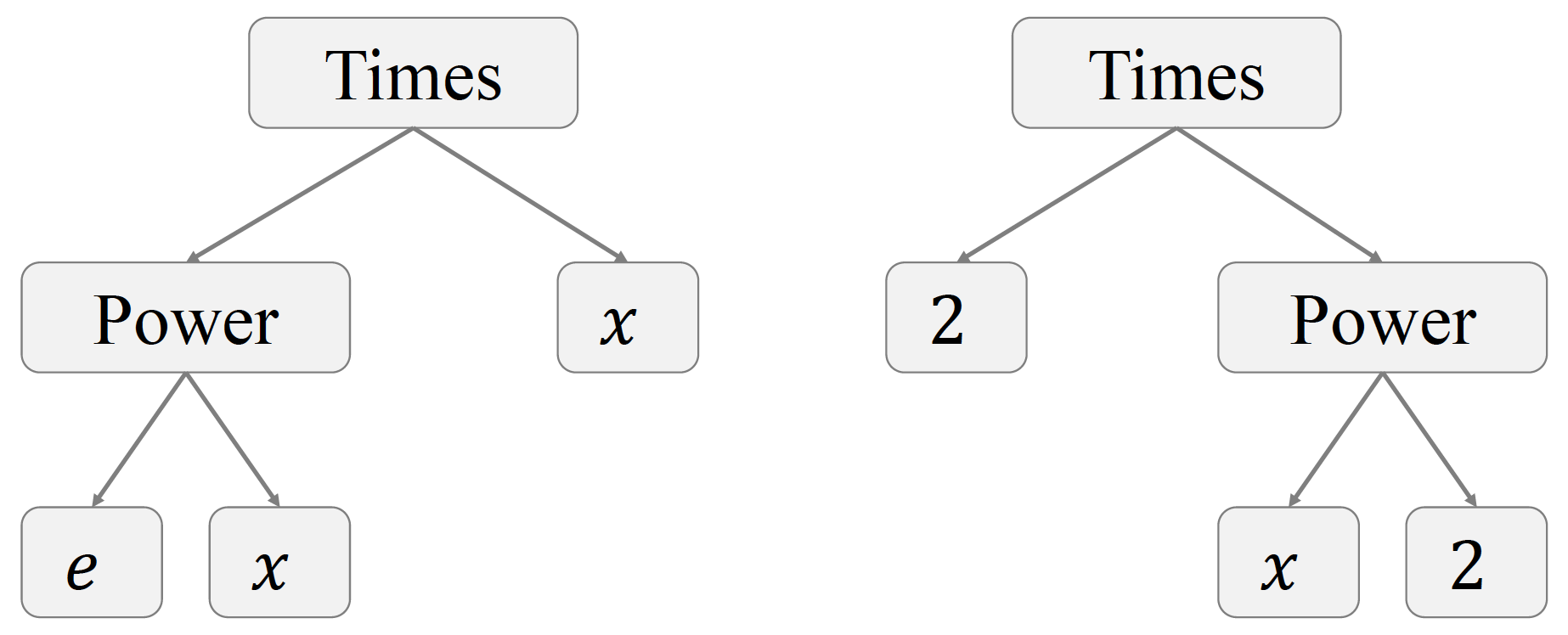
Figure 1: Two exemplifying grammatical expressions corresponding to the individuals $xe^{x}$ and $2x^{2}$.

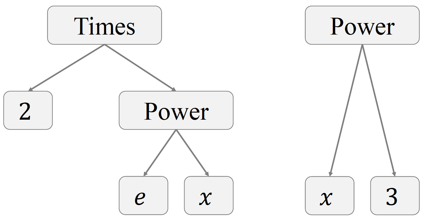
Figure 2: The two selected individuals have been combined to produce two new individuals: $2e^{x}$ and $x^{3}$.

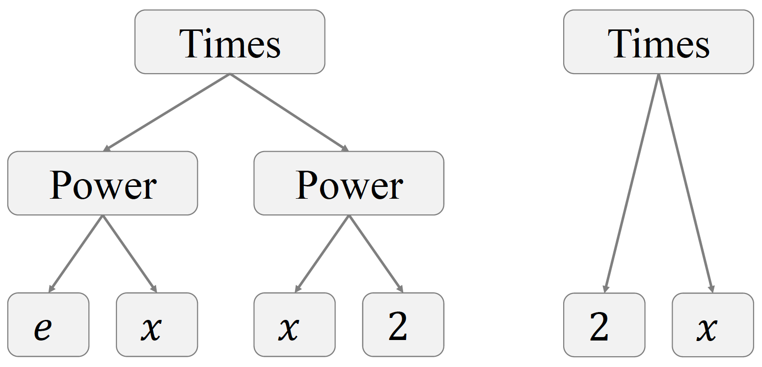
Figure 3: The two selected individuals have suffered a mutation to become two new individuals: $x^{2}e^{x}$ and $2x$.

Now, we describe the way reproduction works in GA with an example. In Fig. 1, there are two expressions in tree representation, i.e., two individuals $xe^{x}$ and $2x^{2}$. Let us assume that these individuals were selected for reproduction. Figure 2 shows possible combinations of the two individuals, while Fig. 3 shows their possible mutations. For instance, the new individual in the left-hand side of Fig. 2 is born from the combination of the expressions $e^{x}$ and $2$ from its parents, while the other individual is made from the remaining parts, $x$ and $x^{2}$, using the proper basic operation “Times” or product. During the mutation stage, a selected individual is altered randomly. As shown in Fig. 3, for instance, the individual $xe^{x}$ mutated to $x^{2}e^{x}$, and the individual $2x^{2}$ mutated to $2x$.

V Results

In this section, we present our fitting formulae for the matter transfer function. We firstly consider the case when $T(k)$ depends only on the amount of baryons and matter, and then we add the effects of massive neutrinos. For both cases, we start describing how the data for the fitting process was gathered using CLASS, and later we proceed to introduce the simple fitting function we found using the GA.

V.1 Baryons and Matter

V.1.1 Data

We use the Boltzmann solver CLASS to compute the linear matter transfer function $T(k)$. In this code, each pair of parameters $\{\omega_{b},\omega_{m}\}$ defines a cosmology for which we can compute the gravitational potential $\Phi$ as a function of the scale $k$ at a fixed redshift. Hence, to see the dependence of the transfer function on these parameters, we make a grid of $4\times 4$ pairs of $\{\omega_{b},\omega_{m}\}$ and compute the gravitational potential for each pair. We consider that $\omega_{b}\in[0.0214,0.0234]$, and $\omega_{m}\in[0.13,0.15]$, which are around $10\sigma$ from the best-fit values found by the Planck Collaboration Planck:2018vyg . For each considered cosmology (16 in total), CLASS retrieves $114$ points $\{k,\Phi\}$. Therefore, our preliminary dataset is composed by 1824 points whose rows are given as $\{k,\omega_{b},\omega_{m},\Phi\}$. Now, since the transfer function is basically the normalized potential, we normalize each of the 16 sub-datasets to get $T(k;\omega_{b},\omega_{m})$. At the end, our final dataset is a table of dimensions $1824\times 4$ with data points given as $\{k,\omega_{b},\omega_{m},T\}$.

	Expression	$\%$ Accuracy
BBKS	Eq. (7)	8.70957
EH	Appendix A	0.777504
GA	Eq. (11)	0.815012

Table 1: Expression and accuracy of the fitting formulae for the matter transfer function as a function of $k$, $\omega_{b}$, and $\omega_{m}$. Although the GA does not provide a more accurate formula than the EH formula, the simplicity of the former [Eq. (11)] is a major improvement over the EH formula (Appendix A).

We quantify the goodness of fit of a given analytical expression by the following function

$$\text{\%Acc}=\frac{100}{N}\sum_{i=1}^{N}\left|\frac{T_{i,\text{CLASS}}-T_{i,\text{analytical}}}{T_{i,\text{CLASS}}}\right|,$$ (8)

where $N=1824$ is the number of data points in our dataset, and $T_{i}$ is a simplified notation for the transfer function evaluated at $k_{i}$, $\omega_{b_{i}}$, and $\omega_{m_{i}}$.

V.1.2 Fitting Formula from the GA

Here, we give a few details concerning the specific GA configuration we used and present our fitting formula.

As explained in Sec. IV, the GA looks for a fitting formula to a dataset by evolving the population, which is composed by expressions combining specific operations (grammar) and coefficients. Schematically, our GA is searching for a function of the form

$$T_{\text{GA}}(x)\equiv\left[1+f_{\text{GA}}(x)\right]^{-1/4},$$ (9)

where

$$x\equiv\frac{k\,\text{Mpc}}{\omega_{m}-\omega_{b}},\quad f_{\text{GA}}\equiv\sum_{i=1}^{4}a_{i}g_{i}\left((b_{i}x)^{c_{i}}\right).$$ (10)

We see that $x$ is a dimensionless quantity since $k$ is given in units $[h\,\text{Mpc}^{-1}]$, $h$ the reduced Hubble parameter. The constants $a_{i}$, $b_{i}$, $c_{i}$ are non-negative random numbers, and $g_{i}$ is an operation in the grammar set, which we consider to be simply of the form $\{x\}$. The quantities $a_{i}$, $g_{i}$, $b_{i}$, and $c_{i}$ are the 4 nucleotides. The sum goes from 1 to 4 because we are considering that the genome of the individuals is formed by 4 genes, each one composed by the 4 nucleotides, such that the chromosomes are $4\times 4$ matrices.

It should be noted that the number of genes has to be fixed before the code starts running and we have chosen the number four for two reasons: i) first, from experience we have found that a number of four genes is a compromise (found by trial and error) on the length of the function, as less than is not enough to fit the data, while a much larger number slows down the code considerably, ii) second, if the number of genes is too high, then this could obviously lead to overfitting or instabilities in the fitting. Furthermore, even though at first sight it seems so, the parameters $a_{i}$ and $b_{i}$, in general are not degenerate as $b_{i}$ appears inside the grammar function, however there may be some degeneracies only when the grammar is linear.

Overall, this configuration, although restrictive, fixes the length of the expressions, thus avoiding over-fitting problems. A couple of reasons motivate the specific forms of Eqs. (9) and (10): $i)$ the transfer function has specific limits: $T\rightarrow 0$ when $k\rightarrow\infty$, and $T\rightarrow 1$ when $k\rightarrow 0$, $ii)$ the transfer function only takes on non-negative values, and $iii)$ $T(k)$ is smooth.

Now, we present our fitting formula when only baryons and matter are considered. Using the configuration of the GA as explained, the stochastic search ended up with the function

$$T_{\text{GA}}(k;\omega_{b},\omega_{m}) =\left[1+59.0998\,x^{1.49177}+4658.01\,x^{4.02755}+3170.79\,x^{6.06}+150.089\,x^{7.28478}\right]^{-1/4},$$ (11)

whose goodness of fit, as measured by Eq. (8), is $\%\text{Acc}_{\text{GA}}=0.815012$. The accuracy of the BBKS formula in Eq. (7) is $\%\text{Acc}_{\text{BBKS}}=8.70957$, and for the EH formula is $\%\text{Acc}_{\text{EH}}=0.777504$. We compile these results in Table 1. In Fig. 4, we compare the performance of the fitting formulae. As it can be seen in the left panel of this figure, the three formulae are very accurate on the large scales ($k<0.01h\,\text{Mpc}^{-1}$), while for smaller scales ($k>0.01h\,\text{Mpc}^{-1}$), where the effects of baryons are most prominent on the cosmological evolution, the accuracy of the three formulae decrease. However, we note that our GA formula and the EH formula can be accurate up to 5%, while the BBKS formula is accurate up to 18% in these scales. We would like to emphasize that our GA formula in Eq. (11) is remarkably simpler than the EH formula which is described by around 30 expressions which occupy the whole Appendix A, while their difference in accumulative accuracy is just about 0.04. We also want to stress that, in principle, the GA could get even better results if some modifications are introduced. For instance, a larger grammar set and a more complex $f_{\text{GA}}$ function [instead of Eq. (10)]. Nonetheless, our choices avoid over-fitting while yielding a smooth transfer function with the correct limits in $k$.

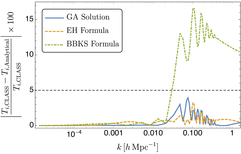
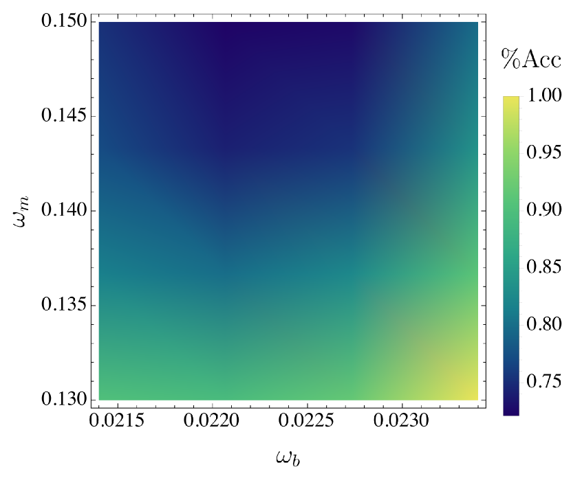
Figure 4: (Left) Accuracy of the BBKS (green dot-dashed line), EH (mustard dashed line), and the GA (blue solid line) fitting formulae as a function of the scale $k$ and fixed $\{\omega_{m},\omega_{b}\}$. The parameters for these plots are: $\omega_{b}=0.02273$, and $\omega_{m}=0.1366$. Note that the accuracy of the three formulae notably decrease on the scales where the effects of baryons are most prominent on the cosmological evolution. However, the accuracy of the EH and GA formulae are below 5% in this scale. (Right) Average accuracy of the GA fitting formula for all $k$ as a function of $\{\omega_{m},\omega_{b}\}$. As it can be seen, the formula is up to $1\%$ accurate in overall.

V.2 Baryons, Matter and Massive Neutrinos

V.2.1 Data

Apart of baryons and cold dark matter, massive neutrinos can contribute to the matter content once they are freely streaming. We can take into account the effects of massive neutrinos in the matter transfer function using CLASS. We compute $T(k)$ at redshift zero as a function of $\omega_{b}$, $\omega_{m}$ in the same ranges as in Sec. V.1, and $\omega_{\nu}\equiv 0.0107(\sum_{\nu}m_{\nu}/1.0\,\text{eV})$, assuming just one massive neutrino, and that the total mass of massive neutrinos is in the range $0.06\,\text{eV}\leq\sum m_{\nu}\leq 0.12\,\mathrm{eV}$. The lower bound of the later constraint corresponds to the minimum mass allowed from neutrino flavour oscillation experiments Lesgourgues:2013sjj , and the upper bound is the maximum mass value allowed by Planck Planck:2018vyg . In this case, we get a grid of $4\times 4\times 4$ data points for $\{\omega_{b},\omega_{m},\omega_{\nu}\}$ and compute the gravitational potential for each triad. Again, for each considered cosmology (64 in total), CLASS retrieves $114$ points $\{k,\Phi\}$. Normalizing the potential to get the transfer function, our final data set is a table of dimensions $7296\times 5$ with data points given as $\{k,\omega_{b},\omega_{m},\omega_{\nu},T\}$. We use Eq. (8) to quantify the goodness of fit of the analytical expressions, but now $N=7296$ is the number of data points in our dataset, and $T_{i}$ is the transfer function evaluated at $k_{i}$, $\omega_{b_{i}}$, $\omega_{m_{i}}$, and $\omega_{\nu_{i}}$.

V.2.2 Fitting Formula from the GA

Based on the success of the GA in finding an accurate formula for $T(k)$ when neutrinos are massless, this time our GA is looking for a function of the form

$$T_{\text{GA}}(y)\equiv\left[1+f_{\text{GA}}(y)\right]^{-1/4},$$ (12)

where

$$y\equiv\frac{k\,\text{Mpc}}{\omega_{m}-\omega_{b}+\omega_{\nu}},\quad f_{\text{GA}}\equiv\sum_{i=1}^{4}a_{i}g_{i}\left((b_{i}y)^{c_{i}}\right).$$ (13)

Now, we present our fitting formula which considers baryons, matter, and one massive neutrino:

$$T_{\text{GA}}(k;\omega_{b},\omega_{m}) =\left[1+56.4933\,y^{1.48261}+3559.23\,y^{3.76407}+4982.44\,y^{5.68246}+374.167\,y^{7.14558}\right]^{-1/4},$$ (14)

whose goodness of fit, as measured by Eq. (8), is $\%\text{Acc}_{\text{GA}}=0.993916$. The accuracy of the extended EH formula considering massive neutrinos is $\%\text{Acc}_{\text{EH}}=1.23449$. We compile these results in Table 2. In Fig. 5, we compare the performance of the fitting formulae. Similar to the last section, the formulae are more accurate on large scales ($k<0.01h\,\text{Mpc}^{-1}$) than on the smaller scales ($k>0.01h\,\text{Mpc}^{-1}$). Note in the left panel of this figure that the accuracy of the GA formula is below the $5\%$ in the whole range of $k$. Furthermore, the GA formula (14) is significantly simpler than the EH formula, whose description requires around 30 expression which we give in full in Appendix B. Our result is a compelling analytical alternative to compute the matter transfer function.

	Expression	$\%$ Accuracy
EH	Appendix B	1.23449
GA	Eq. (14)	0.993916

Table 2: Expression and accuracy of the fitting formulae for the matter transfer function as a function of $k$, $\omega_{b}$, $\omega_{m}$, and $\omega_{\nu}$. Although the accuracy of both formulations are similar, the simplicity of the GA function in Eq. (14) is a major improvement over the EH formula, which is fully displayed in Appendix B.

VI Conclusions

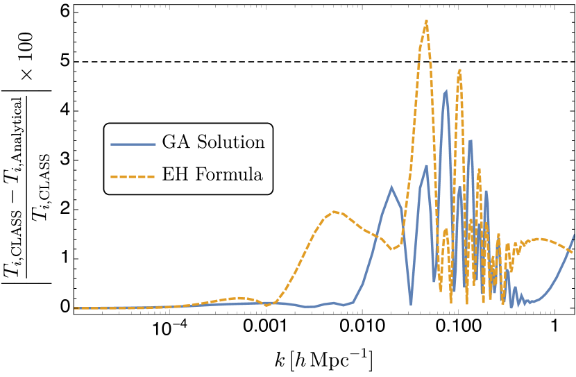
Figure 5: (Left) Accuracy of the EH (mustard dashed line), and the GA (blue solid line) fitting formulae as a function of the scale $k$ for fixed $\{\omega_{m},\omega_{b}\,\omega_{\nu}\}$. The parameters for these plots are: $\omega_{b}=0.02206$, $\omega_{m}=0.1499$, and $\omega_{\nu}=0.0008599$ which corresponds to a mass of $\sum_{\nu}m_{\nu}=0.08\,\text{eV}$. As can be seen, the accuracy of the GA formula is below 5% on the whole range of $k$ considered here. (Right) Average accuracy of the GA fitting formula for all $k$ and $\omega_{\nu}$ as a function of $\{\omega_{m},\omega_{b}\}$. As it can be seen, the formula is around $1\%$ accurate in overall.

Genetic Algorithms (GAs), a machine learning technique, have been previously used to obtain improved formulation of cosmological quantities of interest such as the redshift at recombination and the sound horizon at drag epoch Aizpuru:2021vhd , and also to perform consistency tests to probe for deviations from $\Lambda$CDM Renzi:2020bvl ; EUCLID:2020syl ; Arjona:2020axn ; arjona:2021mzf ; Euclid:2021frk ; Arjona:2021hmg ; Alestas:2022gcg . Here we used the GA to find analytical alternatives to existing fitting functions for the matter transfer function, such as the BBKS and the EH formulae.

When the transfer function depends only on $\omega_{b}$ and $\omega_{m}$, the GA finds a very simple fitting formula for $T(k)$ [see Eq. (11)], which is as accurate as the EH formula, while being significantly shorter (see Appendix A). In a more realistic scenario, at least one neutrino should be massive. In this case, our GA finds a fitting function which is both more accurate and notably simpler [see Eq. (14)] than the EH formula in Appendix B. The simplicity of the GA fitting formulae and their accuracy represent a major improvement over other existing analytical formulations of the matter transfer function which are extensively used in the literature Boyanovsky:2008he ; Dvornik:2022xap ; Schoneberg:2022ggi . Therefore, the GA formulae in Eqs. (11) and (14) are compelling semi-analytic alternatives to easily and accurately compute the matter power spectrum.

Numerical Codes

The genetic algorithm code used here can be found in the GitHub repository https://github.com/BayronO/Transfer-Function-GA of BOQ. This code is based on the GA code by SN which can be found at https://github.com/snesseris/Genetic-Algorithms.

Appendix A EH Formula

The transfer function given by Eisenstein and Hu Eisenstein:1997ik has the following form:

$$T(k)=\frac{\Omega_{b}}{\Omega_{0}}T_{b}(k)+\frac{\Omega_{c}}{\Omega_{0}}T_{c}(k),$$ (15)

where $\Omega_{0}=\Omega_{b}+\Omega_{c}$. The terms involved in this formula are the following:

$$T_{b}=\Bigg{[}\frac{\tilde{T}_{0}(k;1,1)}{1+\left(ks/5.2\right)^{2}}+\frac{\alpha_{b}}{1+\left(\beta_{b}/ks\right)^{3}}e^{-\left(\frac{k}{k_{\mathrm{Silk}}}\right)^{1.4}}\Bigg{]}j_{0}(k\tilde{s}),$$ (16)

$$T_{c}=f\tilde{T}_{0}(k,1,\beta_{c})+(1-f)\tilde{T}_{0}(k,\alpha_{c},\beta_{c}),$$ (17)

$$\tilde{T}_{0}(k,\alpha_{c},\beta_{c})=\frac{\ln(e+1.8\beta_{c}q)}{\ln(e+1.8\beta_{c}q)+Cq^{2}},$$ (18)

$$f =\frac{1}{1+(ks/5.4)^{4}},$$ (19)

$$C =\frac{14.2}{\alpha_{c}}+\frac{386}{1+69.9q^{1.08}},$$ (20)

$$q =\frac{k}{13.41k_{\mathrm{eq}}},$$ (21)

$$R \equiv 3\rho_{b}/4\rho_{\gamma}=31.5\omega_{b}\Theta_{2.7}^{-4}(z/10^{3})^{-1},$$ (22)

$$k_{\mathrm{Silk}} =1.6\omega_{b}^{0.52}\omega_{0}^{0.73}\left[1+\left(10.4\,\omega_{0}\right)^{-0.95}\right]\,\mathrm{Mpc}^{-1},$$ (23)

$$k_{\mathrm{eq}} =7.46\times 10^{-2}\omega_{0}\Theta_{2.7}^{-2}\,\mathrm{Mpc}^{-1},$$ (24)

$$\alpha_{b} =2.07k_{\mathrm{eq}}s(1+R_{d})^{-3/4}G\left(\frac{1+z_{\mathrm{eq}}}{1+z_{d}}\right),$$ (25)

$$\beta_{b} =0.5+\frac{\Omega_{b}}{\Omega_{0}}+\left(3-2\frac{\Omega_{b}}{\Omega_{0}}\right)\sqrt{\left(17.2\,\omega_{0}\right)^{2}+1},$$ (26)

$$\beta_{\mathrm{node}} =8.41\omega_{0}^{0.435},$$ (27)

$$s =\frac{2}{3k_{\mathrm{eq}}}\sqrt{\frac{6}{R_{\mathrm{eq}}}}\ln\frac{\sqrt{1+R_{d}}+\sqrt{R_{d}+R_{\mathrm{eq}}}}{1+\sqrt{R_{\mathrm{eq}}}},$$ (28)

$$\tilde{s} =s\left[1+\left(\frac{\beta_{\mathrm{node}}}{ks}\right)^{3}\right]^{-1/3},$$ (29)

$$G(y) =-6y\sqrt{1+y}$$

$$+y(2+3y)\ln\left(\frac{\sqrt{1+y}+1}{\sqrt{1+y}-1}\right),$$ (30)

$$y \equiv\frac{1+z_{\text{eq}}}{1+z},$$ (31)

$$\alpha_{c} =a_{1}^{-\Omega_{b}/\Omega_{0}}a_{2}^{-(\Omega_{b}/\Omega_{0})^{3}},$$ (32)

$$a_{1} =(46.9\omega_{0})^{0.670}[1+(32.1\omega_{0})^{-0.532}],$$ (33)

$$a_{2} =(12.0\omega_{0})^{0.424}[1+(45.0\omega_{0})^{-0.582}],$$ (34)

$$\beta_{c}^{-1} =1+b_{1}[(\Omega_{c}/\Omega_{0})^{b_{2}}-1],$$ (35)

$$b_{1} =0.944[1+(458\omega_{0})^{-0.708}]^{-1},$$ (36)

$$b_{2} =(0.395\omega_{0})^{-0.0266}.$$ (37)

$$z_{\mathrm{eq}} =2.50\times 10^{4}\omega_{0}\Theta_{2.7}^{-4},$$ (38)

$$z_{d} =1291\frac{\omega_{0}^{0.251}}{1+0.659\omega_{0}^{0.828}}\left[1+b_{1,z}\omega_{b}^{b_{2,z}}\right],$$ (39)

$$b_{1,z} =0.313\omega_{0}^{-0.419}\left[1+0.607\omega_{0}^{0.674}\right],$$ (40)

$$b_{2,z} =0.238\omega_{0}^{0.223},$$ (41)

where we have defined $\omega_{0}=(\Omega_{c}+\Omega_{b})h^{2}$, and $T_{\text{CMB}}\equiv 2.7\Theta_{2.7}\,\text{K}$, $R_{d}\equiv R(z_{d})$ and $R_{\text{eq}}\equiv R(z_{\text{eq}})$

Appendix B EH Formula with Massive Neutrinos

The transfer function given by Eisenstein and Hu considering massive neutrinos has the following form Eisenstein:1997jh :

$$T_{cb\nu}(k,z)=T_{\text{master}}(k)\frac{D_{cb\nu}(k,z)}{D_{1}(z)},$$ (42)

The terms involved in this formula are the following:

$$T_{\text{master}}(k) =T_{\text{sup}}(k)B(k),$$ (43)

$$D_{cb\nu}(z,q) =\left[f_{cb}^{0.7/p_{cb}}+\left(\frac{D_{1}(z)}{1+y_{\text{fs}}(q;f_{\nu})}\right)^{0.7}\right]^{p_{cb}/0.7}$$

$$\times D_{1}(z)^{1-p_{cb}},$$ (44)

$$D_{1}(z) =\left(\frac{1+z_{eq}}{1+z}\right)\frac{5\Omega(z)}{2}\Big{\{}\Omega(z)^{4/7}$$ (45)

$$-\Omega_{\Lambda}(z)+\left[1+\frac{\Omega(z)}{2}\right]\left[1+\frac{\Omega_{\Lambda}(z)}{70}\right]\Big{\}}^{-1},$$

$$\Omega(z) =\Omega_{0}(1+z)^{3}g^{-2}(z),$$ (46)

$$\Omega_{\Lambda}(z) =\Omega_{\Lambda}g^{-2}(z),$$ (47)

$$g^{2}(z) =(1-\Omega_{0}-\Omega_{\Lambda})(1+z)^{2}+\Omega_{0}(1+z)^{3}$$

$$+\Omega_{\Lambda},$$ (48)

$$T_{\text{sup}}(k) =\frac{L}{L+Cq^{2}_{\text{eff}}},$$ (49)

$$L =\ln(e+1.84\beta_{c}\sqrt{\alpha_{\nu}}q_{\text{eff}}),$$ (50)

$$C =14.4+\frac{325}{1+60.5q_{\text{eff}}^{1.08}},$$ (51)

$$\beta_{c} =(1-0.949f_{\nu b})^{-1},$$ (52)

$$y_{\rm fs}(q) =17.2f_{\nu}(1+0.488f_{\nu}^{-7/6})(qN_{\nu}/f_{\nu})^{2},$$ (53)

$$q =\frac{k}{\text{Mpc}^{-1}}\Theta_{2.7}^{2}\omega_{0}^{-1},$$ (54)

$$B(k) =1+\frac{1.24f_{\nu}^{0.64}N_{\nu}^{0.3+0.6f_{\nu}}}{q_{\nu}^{-1.6}+q_{\nu}^{0.8}},$$ (55)

$$q_{\nu} =3.92q\sqrt{\frac{N_{\nu}}{f_{\nu}}}$$ (56)

$$f_{c} =\frac{\Omega_{b}}{\Omega_{m}+\Omega_{\nu}},\quad f_{\nu}=\frac{\Omega_{\nu}}{\Omega_{m}+\Omega_{\nu}},$$

$$f_{cb} =\frac{\Omega_{m}}{\Omega_{m}+\Omega_{\nu}},\quad f_{\nu b}=\frac{\Omega_{b}+\Omega_{\nu}}{\Omega_{m}+\Omega_{\nu}},$$ (57)

$$q_{\text{eff}} =\frac{k\Theta_{2.7}^{2}}{\Gamma_{\text{eff}}\,\text{Mpc}^{-1}},$$ (58)

$$\Gamma_{\text{eff}} =\omega_{0}\left[\sqrt{\alpha_{\nu}}+\frac{1-\sqrt{\alpha_{\nu}}}{1+(0.43ks)^{4}}\right],$$ (59)

$$\alpha_{\nu} =\frac{f_{c}}{f_{cb}}\frac{5-2(p_{c}+p_{cb})}{5-4p_{cb}}$$ (60)

$$\times\frac{1-0.553f_{\nu b}+0.126f_{\nu b}^{3}}{1-0.193\sqrt{f_{\nu}N_{\nu}}+0.169f_{\nu}N_{\nu}^{0.2}}(1+y_{d})^{p_{cb}-p_{c}}$$

$$\times\Big{[}1+\frac{p_{c}-p_{cb}}{2}\left(1+\frac{1}{(3-4p_{c})(7-4p_{cb})}\right)$$

$$\times(1+y_{d})^{-1}\Big{]},$$ (61)

$$p_{c} \equiv\frac{1}{4}\left[5-\sqrt{1+24f_{c}}\right],$$ (62)

$$p_{cb} \equiv\frac{1}{4}\left[5-\sqrt{1+24f_{cb}}\right],$$ (63)

$$z_{\mathrm{eq}} =2.50\times 10^{4}\omega_{0}\Theta_{2.7}^{-4},$$ (64)

$$z_{d} =1291\frac{\omega_{0}^{0.251}}{1+0.659\omega_{0}^{0.828}}\left[1+b_{1,z}\omega_{b}^{b_{2,z}}\right],$$ (65)

$$b_{1} =0.313\omega_{0}^{-0.419}\left[1+0.607\omega_{0}^{0.674}\right],$$ (66)

$$b_{2} =0.238\omega_{0}^{0.223},$$ (67)

$$y \equiv\frac{1+z_{\text{eq}}}{1+z},$$ (68)

$$s =\frac{44.5\ln(9.83\omega_{0})}{\sqrt{1+10\omega_{b}^{3/4}}}\,\text{Mpc},$$ (69)

where $N_{\nu}$ is the number of massive neutrinos, $\Omega_{\Lambda}$ is the density parameter of cosmological constant, and we have redefine some terms like $\Omega_{0}=\Omega_{c}+\Omega_{b}+\Omega_{\nu}$, and $\omega_{0}=\Omega_{0}h^{2}$.

References

- (1) P. J. E. Peebles, Cosmology’s Century: An Inside History of Our Modern Understanding of the Universe. Princeton University Press, 2020.
- (2) Planck Collaboration, N. Aghanim et al., “Planck 2018 results. VI. Cosmological parameters,” Astron. Astrophys. 641 (2020) A6, arXiv:1807.06209 [astro-ph.CO]. [Erratum: Astron.Astrophys. 652, C4 (2021)].
- (3) DES Collaboration, M. A. Troxel et al., “Dark Energy Survey Year 1 results: Cosmological constraints from cosmic shear,” Phys. Rev. D 98 no. 4, (2018) 043528, arXiv:1708.01538 [astro-ph.CO].
- (4) DES Collaboration, T. M. C. Abbott et al., “Dark Energy Survey Year 1 Results: Constraints on Extended Cosmological Models from Galaxy Clustering and Weak Lensing,” Phys. Rev. D 99 no. 12, (2019) 123505, arXiv:1810.02499 [astro-ph.CO].
- (5) DES Collaboration, T. M. C. Abbott et al., “Dark Energy Survey Year 3 results: Cosmological constraints from galaxy clustering and weak lensing,” Phys. Rev. D 105 no. 2, (2022) 023520, arXiv:2105.13549 [astro-ph.CO].
- (6) Supernova Search Team Collaboration, A. G. Riess et al., “Observational evidence from supernovae for an accelerating universe and a cosmological constant,” Astron. J. 116 (1998) 1009–1038, arXiv:astro-ph/9805201.
- (7) Supernova Cosmology Project Collaboration, S. Perlmutter et al., “Measurements of and from 42 high redshift supernovae,” Astrophys. J. 517 (1999) 565–586, arXiv:astro-ph/9812133.
- (8) Supernova Search Team Collaboration, A. G. Riess et al., “Type Ia supernova discoveries at z 1 from the Hubble Space Telescope: Evidence for past deceleration and constraints on dark energy evolution,” Astrophys. J. 607 (2004) 665–687, arXiv:astro-ph/0402512.
- (9) W. percival et al., “Baryon acoustic oscillations in the Sloan Digital Sky Survey Data Release 7 galaxy sample,” Monthly Notices of the Royal Astronomical Society 401 no. 4, (2010) 2148–2168.
- (10) C. Blake et al., “The WiggleZ Dark Energy Survey: mapping the distance-redshift relation with baryon acoustic oscillations,” Monthly Notices of the Royal Astronomical Society 418 no. 3, (2011) 1707–1724.
- (11) E. Aubourg et al., “Cosmological implications of baryon acoustic oscillation measurements,” Phys. Rev. D 92 no. 12, (2015) 123516, arXiv:1411.1074 [astro-ph.CO].
- (12) Boomerang Collaboration, P. de Bernardis et al., “A Flat universe from high resolution maps of the cosmic microwave background radiation,” Nature 404 (2000) 955–959, arXiv:astro-ph/0004404.
- (13) A. H. Jaffe et al., “Recent results from the maxima experiment,” New Astron. Rev. 47 (2003) 727–732, arXiv:astro-ph/0306504.
- (14) Planck Collaboration, Y. Akrami et al., “Planck 2018 results. X. Constraints on inflation,” Astron. Astrophys. 641 (2020) A10, arXiv:1807.06211 [astro-ph.CO].
- (15) Planck Collaboration, Y. Akrami et al., “Planck 2018 results. VII. Isotropy and Statistics of the CMB,” Astron. Astrophys. 641 (2020) A7, arXiv:1906.02552 [astro-ph.CO].
- (16) DES Collaboration, T. M. C. Abbott et al., “Cosmological Constraints from Multiple Probes in the Dark Energy Survey,” Phys. Rev. Lett. 122 no. 17, (2019) 171301, arXiv:1811.02375 [astro-ph.CO].
- (17) A. G. Riess et al., “Large Magellanic Cloud Cepheid Standards Provide a 1% Foundation for the Determination of the Hubble Constant and Stronger Evidence for Physics beyond CDM,” Astrophys. J. 876 no. 1, (2019) 85, arXiv:1903.07603 [astro-ph.CO].
- (18) E. Abdalla et al., “Cosmology intertwined: A review of the particle physics, astrophysics, and cosmology associated with the cosmological tensions and anomalies,” JHEAp 34 (2022) 49–211, arXiv:2203.06142 [astro-ph.CO].
- (19) A. Joyce, L. Lombriser, and F. Schmidt, “Dark Energy Versus Modified Gravity,” Ann. Rev. Nucl. Part. Sci. 66 (2016) 95–122, arXiv:1601.06133 [astro-ph.CO].
- (20) E. Di Valentino et al., “In the realm of the Hubble tension — a review of solutions,” Class. Quant. Grav. 38 no. 15, (2021) 153001, arXiv:2103.01183 [astro-ph.CO].
- (21) L. Heisenberg, H. Villarrubia-Rojo, and J. Zosso, “Simultaneously solving the and tensions with late dark energy,” arXiv:2201.11623 [astro-ph.CO].
- (22) L. Perivolaropoulos and F. Skara, “Challenges for CDM: An update,” New Astron. Rev. 95 (2022) 101659, arXiv:2105.05208 [astro-ph.CO].
- (23) W. Cardona and M. A. Sabogal, “Holographic energy density, dark energy sound speed, and tensions in cosmological parameters: and ,” arXiv:2210.13335 [astro-ph.CO].
- (24) R.-Y. Guo, J.-F. Zhang, and X. Zhang, “Can the tension be resolved in extensions to CDM cosmology?,” JCAP 02 (2019) 054, arXiv:1809.02340 [astro-ph.CO].
- (25) P. Agrawal, F.-Y. Cyr-Racine, D. Pinner, and L. Randall, “Rock ’n’ Roll Solutions to the Hubble Tension,” arXiv:1904.01016 [astro-ph.CO].
- (26) L. Heisenberg and H. Villarrubia-Rojo, “Proca in the sky,” JCAP 03 (2021) 032, arXiv:2010.00513 [astro-ph.CO].
- (27) T. Clifton, P. G. Ferreira, A. Padilla, and C. Skordis, “Modified Gravity and Cosmology,” Phys. Rept. 513 (2012) 1–189, arXiv:1106.2476 [astro-ph.CO].
- (28) L. Heisenberg, R. Kase, and S. Tsujikawa, “Cosmology in scalar-vector-tensor theories,” Phys. Rev. D 98 no. 2, (2018) 024038, arXiv:1805.01066 [gr-qc].
- (29) W. Cardona, J. B. Orjuela-Quintana, and C. A. Valenzuela-Toledo, “An effective fluid description of scalar-vector-tensor theories under the sub-horizon and quasi-static approximations,” JCAP 08 no. 08, (2022) 059, arXiv:2206.02895 [astro-ph.CO].
- (30) A. Heavens et al., “No evidence for extensions to the standard cosmological model,” Phys. Rev. Lett. 119 no. 10, (2017) 101301, arXiv:1704.03467 [astro-ph.CO].
- (31) S. Singh et al., “On the detection of a cosmic dawn signal in the radio background,” arXiv:2112.06778 [astro-ph.CO].
- (32) R. Arjona, A. Melchiorri, and S. Nesseris, “Testing the CDM paradigm with growth rate data and machine learning,” JCAP 05 no. 05, (2022) 047, arXiv:2107.04343 [astro-ph.CO].
- (33) Euclid Collaboration, D. Camarena et al., “Euclid: Testing the Copernican principle with next-generation surveys,” arXiv:2207.09995 [astro-ph.CO].
- (34) W. Cardona, R. Arjona, A. Estrada, and S. Nesseris, “Cosmological constraints with the Effective Fluid approach for Modified Gravity,” JCAP 05 (2021) 064, arXiv:2012.05282 [astro-ph.CO].
- (35) SDSS Collaboration, M. Tegmark et al., “The 3-D power spectrum of galaxies from the SDSS,” Astrophys. J. 606 (2004) 702–740, arXiv:astro-ph/0310725.
- (36) BOSS Collaboration, S. Alam et al., “The clustering of galaxies in the completed SDSS-III Baryon Oscillation Spectroscopic Survey: cosmological analysis of the DR12 galaxy sample,” Mon. Not. Roy. Astron. Soc. 470 no. 3, (2017) 2617–2652, arXiv:1607.03155 [astro-ph.CO].
- (37) S. Dodelson and F. Schmidt, Modern Cosmology. Elsevier Science, 2020.
- (38) D. Blas, J. Lesgourgues, and T. Tram, “The Cosmic Linear Anisotropy Solving System (CLASS). Part II: Approximation schemes,” Journal of Cosmology and Astroparticle Physics 2011 no. 07, 034–034.
- (39) A. Lewis, A. Challinor, and A. Lasenby, “Efficient computation of CMB anisotropies in closed FRW models,” Astrophys. J. 538 (2000) 473–476, arXiv:astro-ph/9911177.
- (40) J. M. Bardeen, J. R. Bond, N. Kaiser, and A. S. Szalay, “The Statistics of Peaks of Gaussian Random Fields,” Astrophys. J. 304 (1986) 15–61.
- (41) M. S. Turner, “The Road to Precision Cosmology,” arXiv:2201.04741 [astro-ph.CO].
- (42) D. J. Eisenstein and W. Hu, “Baryonic features in the matter transfer function,” Astrophys. J. 496 (1998) 605, arXiv:astro-ph/9709112.
- (43) D. Boyanovsky, H. J. de Vega, and N. G. Sanchez, “The dark matter transfer function: free streaming, particle statistics and memory of gravitational clustering,” Phys. Rev. D 78 (2008) 063546, arXiv:0807.0622 [astro-ph].
- (44) A. Dvornik et al., “KiDS-1000: Combined halo-model cosmology constraints from galaxy abundance, galaxy clustering and galaxy-galaxy lensing,” arXiv:2210.03110 [astro-ph.CO].
- (45) N. Schöneberg, L. Verde, H. Gil-Marín, and S. Brieden, “BAO+BBN revisited – Growing the Hubble tension with a 0.7km/s/Mpc constraint,” arXiv:2209.14330 [astro-ph.CO].
- (46) G. Carleo et al., “Machine learning and the physical sciences,” Rev. Mod. Phys. 91 no. 4, (2019) 045002, arXiv:1903.10563 [physics.comp-ph].
- (47) M. Schmidt and H. Lipson, “Distilling Free-Form Natural Laws from Experimental Data,” Science 324 (2009) 81–85.
- (48) S. L. Brunton, J. L. Proctor, and J. N. Kutz, “Discovering governing equations from data by sparse identification of nonlinear dynamical systems,” Proceedings of the National Academy of Sciences 113 no. 15, (2016) 3932–3937, arXiv:1509.03580 [math.DS].
- (49) D. Izzo, F. Biscani, and A. Mereta, “Differentiable Genetic Programming,” arXiv e-prints (2016) , arXiv:1611.04766 [cs.NE].
- (50) S.-M. Udrescu and M. Tegmark, “AI Feynman: a Physics-Inspired Method for Symbolic Regression,” Sci. Adv. 6 no. 16, (2020) eaay2631, arXiv:1905.11481 [physics.comp-ph].
- (51) M. Cranmer et al., “Discovering Symbolic Models from Deep Learning with Inductive Biases,” arXiv:2006.11287 [cs.LG].
- (52) Z. Liu and M. Tegmark, “Machine Learning Hidden Symmetries,” Phys. Rev. Lett. 128 no. 18, (2022) 180201, arXiv:2109.09721 [cs.LG].
- (53) J. Koza and J. Koza, Genetic Programming: On the Programming of Computers by Means of Natural Selection. Bradford, 1992.
- (54) R. Arjona and S. Nesseris, “Hints of dark energy anisotropic stress using Machine Learning,” JCAP 11 (2020) 042, arXiv:2001.11420 [astro-ph.CO].
- (55) EUCLID Collaboration, M. Martinelli et al., “Euclid: Forecast constraints on the cosmic distance duality relation with complementary external probes,” Astron. Astrophys. 644 (2020) A80, arXiv:2007.16153 [astro-ph.CO].
- (56) R. Arjona and S. Nesseris, “Novel null tests for the spatial curvature and homogeneity of the Universe and their machine learning reconstructions,” Phys. Rev. D 103 no. 10, (2021) 103539, arXiv:2103.06789 [astro-ph.CO].
- (57) Euclid Collaboration, M. Martinelli et al., “Euclid: Constraining dark energy coupled to electromagnetism using astrophysical and laboratory data,” Astron. Astrophys. 654 (2021) A148, arXiv:2105.09746 [astro-ph.CO].
- (58) A. Aizpuru, R. Arjona, and S. Nesseris, “Machine learning improved fits of the sound horizon at the baryon drag epoch,” Phys. Rev. D 104 no. 4, (2021) 043521, arXiv:2106.00428 [astro-ph.CO].
- (59) Euclid Collaboration, S. Nesseris et al., “Euclid: Forecast constraints on consistency tests of the CDM model,” Astron. Astrophys. 660 (2022) A67, arXiv:2110.11421 [astro-ph.CO].
- (60) G. Alestas, L. Kazantzidis, and S. Nesseris, “Machine learning constraints on deviations from general relativity from the large scale structure of the Universe,” arXiv:2209.12799 [astro-ph.CO].
- (61) B. A. Reid. et al., “Cosmological constraints from the clustering of the Sloan Digital Sky Survey DR7 luminous red galaxies,” Mon. Not. Roy. Astron. Soc. 404 no. 1, (2010) 60–85, arXiv:0907.1659 [astro-ph.CO].
- (62) A. Díaz Rivero, C. Dvorkin, F.-Y. Cyr-Racine, J. Zavala, and M. Vogelsberger, “Gravitational Lensing and the Power Spectrum of Dark Matter Substructure: Insights from the ETHOS N-body Simulations,” Phys. Rev. D 98 no. 10, (2018) 103517, arXiv:1809.00004 [astro-ph.CO].
- (63) S. Chabanier, M. Millea, and N. Palanque-Delabrouille, “Matter power spectrum: from Ly forest to CMB scales,” Mon. Not. Roy. Astron. Soc. 489 no. 2, (2019) 2247–2253, arXiv:1905.08103 [astro-ph.CO].
- (64) J. Lesgourgues, G. Mangano, G. Miele, and S. Pastor, Neutrino Cosmology. Cambridge University Press, 2, 2013.
- (65) KATRIN Collaboration, M. Aker et al., “Direct neutrino-mass measurement with sub-electronvolt sensitivity,” Nature Phys. 18 no. 2, (2022) 160–166, arXiv:2105.08533 [hep-ex].
- (66) D. J. Eisenstein and W. Hu, “Power spectra for cold dark matter and its variants,” Astrophys. J. 511 (1997) 5, arXiv:astro-ph/9710252.
- (67) J. R. Bond and A. S. Szalay, “The collisionless damping of density fluctuations in an expanding universe,” Astrophys. J., Lett. Ed. 274 (1983) 443–468.
- (68) J. R. Bond and G. Efstathiou, “Cosmic background radiation anisotropies in universes dominated by nonbaryonic dark matter,” Astrophys. J., Lett. Ed. 285 (1984) L45–L48.
- (69) E. W. Kolb and M. S. Turner, The Early Universe, vol. 69. Front. Phys., 1990.
- (70) B. C. Allanach, D. Grellscheid, and F. Quevedo, “Genetic algorithms and experimental discrimination of SUSY models,” JHEP 07 (2004) 069, arXiv:hep-ph/0406277.
- (71) Y. Akrami, P. Scott, J. Edsjo, J. Conrad, and L. Bergstrom, “A Profile Likelihood Analysis of the Constrained MSSM with Genetic Algorithms,” JHEP 04 (2010) 057, arXiv:0910.3950 [hep-ph].
- (72) S. Abel, D. G. Cerdeño, and S. Robles, “The Power of Genetic Algorithms: what remains of the pMSSM?,” arXiv:1805.03615 [hep-ph].
- (73) X.-L. Luo, J. Feng, and H.-H. Zhang, “A genetic algorithm for astroparticle physics studies,” Comput. Phys. Commun. 250 (2020) 106818, arXiv:1907.01090 [astro-ph.HE].
- (74) M. Ho et al., “A Robust and Efficient Deep Learning Method for Dynamical Mass Measurements of Galaxy Clusters,” Astrophys. J. 887 (2019) 25, arXiv:1902.05950 [astro-ph.CO].
- (75) C. Bogdanos and S. Nesseris, “Genetic Algorithms and Supernovae Type Ia Analysis,” JCAP 05 (2009) 006, arXiv:0903.2805 [astro-ph.CO].
- (76) S. Nesseris and A. Shafieloo, “A model independent null test on the cosmological constant,” Mon. Not. Roy. Astron. Soc. 408 (2010) 1879–1885, arXiv:1004.0960 [astro-ph.CO].
- (77) S. Nesseris and J. Garcia-Bellido, “A new perspective on Dark Energy modeling via Genetic Algorithms,” JCAP 11 (2012) 033, arXiv:1205.0364 [astro-ph.CO].
- (78) S. Nesseris and J. García-Bellido, “Comparative analysis of model-independent methods for exploring the nature of dark energy,” Phys. Rev. D 88 no. 6, (2013) 063521, arXiv:1306.4885 [astro-ph.CO].
- (79) D. Sapone, E. Majerotto, and S. Nesseris, “Curvature versus distances: Testing the FLRW cosmology,” Phys. Rev. D 90 no. 2, (2014) 023012, arXiv:1402.2236 [astro-ph.CO].
- (80) R. Arjona and S. Nesseris, “What can Machine Learning tell us about the background expansion of the Universe?,” Phys. Rev. D 101 no. 12, (2020) 123525, arXiv:1910.01529 [astro-ph.CO].
- (81) VIRGO Consortium Collaboration, R. E. Smith, J. A. Peacock, A. Jenkins, S. D. M. White, C. S. Frenk, F. R. Pearce, P. A. Thomas, G. Efstathiou, and H. M. P. Couchmann, “Stable clustering, the halo model and nonlinear cosmological power spectra,” Mon. Not. Roy. Astron. Soc. 341 (2003) 1311, arXiv:astro-ph/0207664.
- (82) F. Renzi, N. B. Hogg, M. Martinelli, and S. Nesseris, “Strongly lensed supernovae as a self-sufficient probe of the distance duality relation,” Phys. Dark Univ. 32 (2021) 100824, arXiv:2010.04155 [astro-ph.CO].
- (83) R. Arjona, H.-N. Lin, S. Nesseris, and L. Tang, “Machine learning forecasts of the cosmic distance duality relation with strongly lensed gravitational wave events,” Phys. Rev. D 103 no. 10, (2021) 103513, arXiv:2011.02718 [astro-ph.CO].