Abstract

In this paper, we extend Mazet’s Maximum Principle at infinity for parabolic, two-sided, properly embedded minimal hypersurfaces, up to ambient dimension seven. Parabolicity is a necessary condition in dimension $n\geq 4$, even in Euclidean space, as the example of the higher-dimensional catenoid shows. Next, inspired by the Tubular Neighborhood Theorem of Meeks-Rosenberg in Euclidean three-space we focus on the existence of an embedded $\epsilon-$tube when the ambient manifold $\mathcal{M}$ has non-negative Ricci curvature. These results will allow us to establish Frankel-type properties and to extend the Anderson-Rodríguez Splitting Theorem under the existence of an area-minimizing ${\rm mod}(2)$ hypersurface $\Sigma$ in these manifolds $\mathcal{M}$ (up to dimension seven), the universal covering space of $\mathcal{M}$ is isometric to $\Sigma\times\hbox{\bb R}$ with the product metric. Also, using the recent classification of complete orientable stable hypersurfaces in $\hbox{\bb R}^{4}$ by Chodosh-Li, we are able to show a splitting theorem for $4-$manifolds with non-negative Ricci curvature, scalar curvature bigger than a positive constant and the existence of a non-separating, proper, quasi-embedded hypersurface.

1 Introduction

In this paper we study complete minimal hypersurfaces $\Sigma$ in Riemannian $n-$manifolds $\mathcal{M}^{n}$, $4\leq n\leq 7$, and we obtain some results in the spirit of work we know when $n\leq 3$. The recent papers [12, 13] inspired this endeavor (see also [7] for an alternative proof).

In 1897, J. Hadamard [23] proved two geodesics on a strictly convex $2-$sphere must intersect if one of them is compact. The closure of an embedded complete geodesic is a geodesic lamination. In the Appendix, we prove a geodesic lamination of a strictly convex $2-$sphere is one embedded compact geodesic (recall a lamination is closed). Hence an embedded complete geodesic on such a $2-$sphere (e.g., an ellipsoid) is a compact (circle) geodesic. When $n=3$, we have:

Theorem [45]. Let $\mathcal{M}^{3}$ be a closed orientable manifold with positive Ricci curvature, $\overline{Ric}>0$. If $\Sigma$ is an injectively immersed complete orientable minimal surface of bounded curvature in $\mathcal{M}^{3}$, then $\Sigma$ is compact.

The idea behind these theorems is when the closure of a minimal hypersurface $\Sigma$ is a minimal lamination $\mathcal{L}$, then $\Sigma$ is properly embedded or there is a limit leaf $L\in\mathcal{L}$ ($L$ may be $\Sigma$) that is stable. The ambient geometry and knowledge of stable minimal hypersurfaces exclude the existence of $L$.

To exclude $L$ there are two problems that arise:

• When do two minimal hypersurfaces of $\mathcal{M}^{n}$ necessarily intersect?

• When do two minimal hypersurfaces satisfies a Maximum Principle at Infinity: if $\Sigma_{1}\cap\Sigma_{2}=\emptyset$ then ${\rm dist}_{\mathcal{M}}(\Sigma_{1},\Sigma_{2})>0$?

T. Frankel [21] considered a complete $n-$manifold $\mathcal{M}^{n}$ with positive Ricci curvature, and two minimal hypersurfaces $\Sigma_{1}$ and $\Sigma_{2}$ in $\mathcal{M}^{n}$, $\Sigma_{1}$ closed, $\Sigma_{2}$ immersed and $\overline{\Sigma}_{2}=\Sigma_{2}$. He proved $\Sigma_{1}\cap\Sigma_{2}\neq\emptyset$. C. Croke and B. Kleiner [15] considered two closed orientable embedded minimal hypersurfaces in an orientable complete $\mathcal{M}^{n}$ with non-negative Ricci curvature. They proved that if $\Sigma_{1}$ does not intersect $\Sigma_{2}$ then they are both totally geodesic and (i) or (ii) holds:

1. either $\Sigma_{1}\cup\Sigma_{2}$ bounds a domain in $\mathcal{M}$ isometric to $\Sigma_{1}\times[0,{\bf d}]$, with the product metric, ${\bf d}:={\rm dist}_{\mathcal{M}}(\Sigma_{1},\Sigma_{2})$;

2. or $\mathcal{M}$ is a mapping torus; i.e., $\mathcal{M}$ is isometric to $\Sigma\times[0,{\bf d}]$, with the product metric, where $\Sigma\times\left\{0\right\}$ is identified with $\Sigma\times\left\{{\bf d}\right\}$ by an isometry.

A property that obliges submanifolds to intersect is now known as a Frankel property. Thus the space of closed minimal hypersurfaces in $\mathcal{M}^{n}$ with positive Ricci curvature satisfies the Frankel property and, nowadays, this is well understood if the ambient manifold has non-negative Ricci curvature, $\overline{Ric}\geq 0$, and one of the minimal hypersurfaces is compact (see [14] for a detailed exposition and references therein). When the minimal hypersurfaces are complete and non-compact we refer to the papers [22, 45].

Let $\Sigma$ be a properly immersed minimal surface in $\hbox{\bb R}^{3}$. Then, when $S$ is a properly immersed minimal surface in $\hbox{\bb R}^{3}\setminus\Sigma$, then $\Sigma$ and $S$ are parallel planes (see [39]). A special case of this is the Half-space Theorem of Hoffman-Meeks [25], where $\Sigma$ is a plane of $\hbox{\bb R}^{3}$. An important tool for these questions is a Maximum Principle at Infinity for minimal hypersurfaces. Many people have proved such Maximum Principles (see [28, 33, 39, 43, 47] and references therein), and the most general for us was done by L. Mazet; he proved

Theorem A ([33]): Let $\mathcal{M}^{3}$ be a complete manifold of bounded geometry. Suppose $\Sigma^{2}\subset\mathcal{M}^{3}$ is a two-sided properly embedded minimal surface that has an $\epsilon-$tubular neighborhood ${\rm Tub}_{\epsilon}(\Sigma)$ that is embedded, well-oriented and of bounded extrinsic geometry. If $\Sigma$ is parabolic then the Maximum Principle at Infinity holds for $\Sigma$; i.e., if $S$ is a proper minimal surface such that $\Sigma\cap S=\emptyset$ and $S\cap{\rm Tub}_{\epsilon}(\Sigma)\neq\emptyset$, then $S$ is an equidistant of $\Sigma$.

Remark 1.1.

In fact, L. Mazet proved a mean curvature such theorem. The questions we posed have also been studied for constant mean curvature hypersurfaces with much success. See [33] and references therein.

Here, some definitions are in order.

Definition 1.1.

Let $\mathcal{M}$ be a complete manifold and $\Sigma\subset\mathcal{M}$ be a two-sided embbeded hypersurface. An $\epsilon-$tube is the set of points in $\mathcal{M}$ at distance at most $\epsilon$, that is,

$${\rm Tub}_{\epsilon}(\Sigma)=\left\{p\in\mathcal{M}\,:\,\,{\rm dist}_{\mathcal{M}}(p,\Sigma)\leq\epsilon\right\}.$$

Moreover, ${\rm Tub}_{\epsilon}(\Sigma)$ is:

1. $\epsilon-$Embedded: If the map $F:\Sigma\times[-\epsilon,\epsilon]\to{\rm Tub}_{\epsilon}(\Sigma)$ given by $F(p,t):={\rm exp}_{p}(tN(p))$ is an embedding. Here, ${\rm exp}$ is the exponential map of $\mathcal{M}$ and $N$ is a unit normal along $\Sigma$.

2. Well-oriented: Each equidistant, $\Sigma(\epsilon^{\prime})=\left\{p\in\mathcal{M}\,:\,\,{\rm dist}_{\mathcal{M}}(p,\mathcal{M})=\epsilon^{\prime}\right\}$, at distance $\epsilon^{\prime}\in[-\epsilon,\epsilon]\setminus\left\{0\right\}$ is mean convex (non-negative mean curvature) with the orientation that points away from $\Sigma$.

3. Bounded extrinsic geometry: There exist constants $C,k>0$ so that $\Sigma(\epsilon^{\prime})$ is $k-$quasi-isometric to $\Sigma$ with second fundamental form uniformly bounded by $C$ for all $\epsilon^{\prime}\in[-\epsilon,\epsilon]$.

The idea to prove Theorem A goes as follows. If $S\cap{\rm Tub}_{\epsilon}(\Sigma)\neq\emptyset$ one finds a component $S_{1}\subset S\cap{\rm Tub}_{\epsilon}(\Sigma)$ below $\Sigma(\epsilon_{1})$ and $\partial S_{1}\subset\Sigma(\epsilon_{1})$ for some $\epsilon_{1}<\epsilon$. Then, one has three possibilities:

1. $S_{1}$ is compact: Then the Maximum Principle at the lowest point of $S_{1}$ shows that $S_{1}$ is the equidistant through this point.

2. $S_{1}$ is non-compact and stable: In this case, we have curvature estimates away from the boundary [54] and hence, we can find $\epsilon_{2}\in(0,\epsilon_{1})$, so that a (non-compact) connected component $S_{2}\subset S_{1}\cap{\rm Tub}_{\epsilon_{2}}(\Sigma)$, $\partial S_{2}\subset\Sigma(\epsilon_{2})$, is a graph (in Fermi coordinates) of bounded slope over $\Sigma$. This implies that $S_{2}$ is quasi-isometric to $\Sigma$ and, since $\Sigma$ is parabolic, $S_{2}$ is parabolic with boundary. One then constructs a superharmonic function $h$ on $S_{2}$ of the form $f\circ d$, where $d:={\rm dist}_{\mathcal{M}}(\cdot,\Sigma)$. Then, $h$ must be constant, a contradiction. So $S$ is an equidistant to $\Sigma$.

3. $S_{1}$ is non-compact and not stable: Then, one shows there is a stable surface $\tilde{S}$ below $S_{1}$ in some ${\rm Tub}_{\epsilon_{3}}(\Sigma)\setminus\Sigma$ such that $\partial\tilde{S}\subset\Sigma(\epsilon_{3})$. As above, this gives that the original $S$ is an equidistant to $\Sigma$.

In $\hbox{\bb R}^{3}$ we have the following Maximum Principle at Infinity:

Theorem [39]. Let $\Sigma_{1}$ and $\Sigma_{2}$ be properly immersed minimal surfaces in $\hbox{\bb R}^{3}$, and $\partial\Sigma_{1}\neq\emptyset$. Then

$${\rm dist}_{\hbox{\bbp R}^{3}}(\Sigma_{1},\Sigma_{2})={\rm min}\left\{{\rm dist}_{\hbox{\bbp R}^{3}}(\Sigma_{1},\partial\Sigma_{2}),{\rm dist}_{\hbox{\bbp R}^{3}}(\Sigma_{2},\partial\Sigma_{1})\right\}.$$

Hence if $\partial\Sigma_{1}=\partial\Sigma_{2}=\emptyset$, remove a small disk $D$ from $\Sigma_{1}$ and consider $\tilde{\Sigma}_{1}=\Sigma_{1}\setminus D$ and $\Sigma_{2}$. We conclude: if $\Sigma_{1}\cap\Sigma_{2}=\emptyset$ then ${\rm dist}_{\hbox{\bbp R}^{3}}(\Sigma_{1},\Sigma_{2})>0$. In other words, they are not asymptotic at infinity. Hoffman and Meeks [25] proved $\Sigma_{1}$ and $\Sigma_{2}$ are two properly immersed minimal surfaces such that $\partial\Sigma_{1}=\partial\Sigma_{2}=\emptyset$, then they are parallel planes; their Strong Half-space Theorem. They construct an orientable complete least area surface $L$ between $\Sigma_{1}$ and $\Sigma_{2}$; $L$ is stable hence a plane and they conclude with their Half-space Theorem.

There are many very interesting papers on the Frankel Property and a Maximum Principle at Infinity (see [14] for a detailed exposition and references therein). Understanding stable minimal hypersurfaces is the foundation of the subject.

A complete orientable stable minimal surface in $\hbox{\bb R}^{3}$ is a flat plane [6, 20, 42]. R. Schoen [49] used this to prove an oriented stable complete minimal surface $\Sigma$ in a complete $3-$manifold $\mathcal{M}^{3}$ of bounded geometry has bounded curvature. That is, there exists a constant $\Lambda>0$, depending on $\mathcal{M}^{3}$, such that if $\Sigma$ is as above then

$$|A(x)|{\rm dist}_{\Sigma}(x,\partial\Sigma)\leq\Lambda,\text{ for all }x\in\Sigma,$$

here $|A|$ is the norm of the second fundamental form of $\Sigma$. Thus, $\Sigma$ has bounded curvature at any point of fixed positive distance from $\partial\Sigma$.

Remark 1.2.

Schoen’s curvature estimate depends also on an upper bound on the covariant derivate of the curvature tensor. H. Rosenberg, R. Souam and E. Toubiana [48] obtained such a curvature estimate assuming only a bound on the sectional curvature.

These results are, we believe, of the upmost importance for the study of complete minimal surfaces in $3-$manifolds. To construct examples we can solve Plateau problems for a compact cycle boundary and pass to the limit as the boundaries tend to infinity. The curvature estimates for the Plateau solutions (they are stable) are fundamental to make this work. To understand the global geometry of complete minimal surfaces we use stable surfaces to control the asymptotic geometry. A Maximum Principle at Infinity for two ends of minimal surfaces depends on the curvature estimates.

Recently O. Chodosh and C. Li [12] proved that an orientable, complete, stable, minimal hypersurface in $\hbox{\bb R}^{4}$ is a flat ($\hbox{\bb R}^{3}$) hyperplane. Then, in joint work with D. Stryker, they proved:

Theorem [13]. Let $\mathcal{M}^{4}$ be a complete Riemannian $4-$manifold of bounded geometry. Assume the sectional curvatures of $\mathcal{M}$ are non-negative and the scalar curvature is strictly positive and away from zero. If $\Sigma$ is a two-sided, complete, stable minimal hypersurface in $\mathcal{M}^{4}$ then $\Sigma$ is totally geodesic and the Ricci curvature of the ambient manifold vanishes along $\Sigma$ in the normal direction.

An important consequence of the above result is that such a stable minimal hypersurface must be parabolic; this follows from [41, Theorem 1.2].

Chodosh, Li and Stryker [13] used this to study stable minimal hypersurfaces in certain complete Riemannian $4-$manifolds $\mathcal{M}^{4}$ (not the same manifolds as the theorem above). When the sectional curvatures, $\overline{K}_{ij}$, of $\mathcal{M}^{4}$ satisfy $|\overline{K}_{ij}|\leq C$; for some $C>0$, then one has curvature estimates for two sided stable minimal hypersurfaces $\Sigma^{3}\subset\mathcal{M}^{4}$, applying the “stable implies flat” theorem in $\hbox{\bb R}^{4}$ and a blow-up argument to obtain

$$|A(x)|{\rm dist}_{\Sigma}(x,\partial\Sigma)\leq\Lambda(C),\text{ for all }x\in\Sigma,$$

in particular, a two-sided, complete, stable minimal hypersurface in such $\mathcal{M}^{4}$ has bounded curvature, the bound depending on the geometry of $\mathcal{M}^{4}$ and the distance to the boundary (if the boundary exists). Previous results on curvature estimates in dimensions greater than three were obtained assuming volume growth hypothesis [50, 52]. Examples of such manifolds can be found in [13, 53] and properly embedded minimal hypersurfaces in manifolds of non-negative Ricci curvature were constructed in [17, 18].

We first observe that Theorem A can be extended up to dimension seven with the same techniques, thanks to the Schoen-Simon-Yau’s curvature estimates [50, 52] and the regularity theory for area-minimizers developed by the combined works of De Giorgi, Federer, Fleming, Hardt and Simon (cf. [56, Section 3]), specifically:

Theorem $\tilde{{\rm\bf A}}$: Let $\mathcal{M}^{n}$ , $3\leq n\leq 7$, be a complete manifold of bounded geometry. Suppose $\Sigma^{n-1}\subset\mathcal{M}^{n}$ is a two-sided properly embedded minimal hypersurface that has an $\epsilon-$tubular neighborhood ${\rm Tub}_{\epsilon}(\Sigma)$ that is embedded, well-oriented and of bounded extrinsic geometry. If $\Sigma$ is parabolic then the Maximum Principle at Infinity holds for $\Sigma$; i.e., if $S$ is a proper minimal hypersurface such that $\Sigma\cap S=\emptyset$ and $S\cap{\rm Tub}_{\epsilon}(\Sigma)\neq\emptyset$, then $S$ is an equidistant of $\Sigma$.

In order to prove the Theorem $\tilde{{\rm A}}$ one must prove that area-minimizing ${\rm mod}(2)$ hypersurfaces have curvature estimates only depending on the ambient manifold and distance to the boundary when $n\leq 7$. This is done in detail in Section 3. Parabolicity is a necessary condition in dimension $n\geq 4$, even in Euclidean space, as the example of the catenoid shows.

In Section 4, inspired by the Tubular Neighborhood Theorem of Meeks-Rosenberg in Euclidean three-space [39, 45], we focus on the existence of an embedded $\epsilon-$tube when the ambient manifold has non-negative Ricci curvature.

Theorem 4.1 (Tubular Neighborhood Theorem): Let $(\mathcal{M}^{n},g)$, $3\leq n\leq 7$, be a complete orientable manifold of bounded geometry and $\overline{Ric}\geq 0$. Let $\Sigma\subset\mathcal{M}$ be a properly embedded, orientable, parabolic, minimal hypersurface of bounded second fundamental form. Then, there exists $\epsilon>0$ (depending only on the bounds for the sectional curvatures and the second fundamental form) such that ${\rm Tub}_{\epsilon}(\Sigma)$ is embedded. Moreover, ${\rm Tub}_{\epsilon}(\Sigma)$ is well-oriented and of bounded extrinsic geometry (cf. Definition 1.1).

In Euclidean $n-$space, $n\geq 4$, there are no parabolic, complete, minimal hypersurfaces by the monotonicity formula.

In Section 5 we restrict to $4-$manifolds of non-negative sectional curvatures and scalar curvature bounded below by a positive constant. Under these conditions, stable, two-sided minimal hypersurfaces are totally geodesic and parabolic (cf. [13]). The existence of a non-separating, properly quasi-embedded minimal hypersuface in such manifolds implies a local splitting. We shall explain the meaning of quasi-embedded:

Definition 1.2.

Let $\Sigma\subset\mathcal{M}$ be a properly immersed, two-sided, hypersurface in a complete manifold $\mathcal{M}$. $\Sigma$ is said properly quasi-embedded if there exists a compact set $\mathcal{K}\subset\mathcal{M}$ such that $\Sigma\setminus\mathcal{K}$ is embedded.

The above definition leads us to:

Definition 1.3.

Let $\Sigma\subset\mathcal{M}$ be a properly quasi-embedded hypersurface. We say that $\Sigma$ is non-separating if for $p\in\Sigma\setminus\mathcal{K}$, the embedded part of $\Sigma$, there exists a simple closed curve $\gamma\subset\mathcal{M}$ intersecting $\Sigma$ transversally in the one point $p$.

The above results imply that, when a two-sided, complete, stable minimal hypersurface in such an $\mathcal{M}^{4}$ is parabolic; such parabolic minimal hypersurfaces satisfy the Maximum Principle at Infinity (Theorem $\tilde{\text{A}}$), and this enable us to prove a Splitting Theorem.

Theorem 5.1: Let $(\mathcal{M}^{n},g)$, $n=4$, be a complete orientable manifold of bounded geometry, $\overline{K}_{ij}\geq 0$ and $\overline{Sc}\geq c>0$. Let $\Sigma\subset\mathcal{M}$ be a properly quasi-embedded, orientable, minimal hypersurface. Assume $\Sigma$ does not separate, then:

• $\Sigma$ is embedded.

• $\mathcal{M}$ is a mapping torus; i.e., $\mathcal{M}$ is isometric to $\Sigma\times[0,{\bf d}]$, with the product metric, where $\Sigma\times\left\{0\right\}$ is identified with $\Sigma\times\left\{{\bf d}\right\}$ by an isometry.

• If $\tilde{\Sigma}$ is an orientable, properly immersed minimal hypersurface in $\mathcal{M}\setminus\Sigma$, then $\tilde{\Sigma}=\Sigma\times\left\{t\right\}$ for some $t\in[0,{\bf d}]$.

This also enable us to prove a Frankel-type property in these manifolds:

Corollary 5.2: Let $(\mathcal{M}^{n},g)$, $n=4$, be a complete orientable manifold of bounded geometry, $\overline{K}_{ij}\geq 0$ and $\overline{Sc}\geq c>0$. Let $\Sigma_{1},\Sigma_{2}\subset\mathcal{M}$ be two properly quasi-embedded, orientable, minimal hypersurfaces. Then, either $\Sigma_{1}$ intersects $\Sigma_{2}$ or they are embedded and parallel.

We shall explain here the meaning of parallel in a Riemannian manifold.

Definition 1.4.

Let $\mathcal{M}^{n}$ be a complete Riemannian manifold. We say that two disjoint properly embedded hypersurfaces $\Sigma_{1},\Sigma_{2}\subset\mathcal{M}$ are parallel if there exists a domain $\mathcal{U}\subset\mathcal{M}\setminus\left(\Sigma_{1}\cup\Sigma_{2}\right)$ such that $\partial\mathcal{U}=\Sigma_{1}\cup\Sigma_{2}$ and $\overline{\mathcal{U}}$ is a product manifold over $\Sigma_{1}$ (or $\Sigma_{2}$); i.e, $\overline{\mathcal{U}}=\Sigma_{1}\times[0,{\bf d}]$ endowed with the product metric. Here ${\bf d}:={\rm dist}_{\mathcal{M}}(\Sigma_{1},\Sigma_{2})>0$ and $\Sigma_{2}=\Sigma_{1}\times\left\{{\bf d}\right\}$.

Remark 1.3.

Usually, parallel means that the distance between the two hypersurfaces is constant. For us, to be parallel is a stronger condition, we also ask that between the hypersurfaces the manifold has a product structure.

An interesting subject of future research is the study of properly embedded minimal (and CMC) hypersurfaces in $\hbox{\bb S}^{2}\times\hbox{\bb R}^{2}$ with the product metric, $\hbox{\bb S}^{2}$ the standard $2-$sphere of curvature one, and $\hbox{\bb T}^{2}\times\hbox{\bb R}^{2}$ with the product metric, $\hbox{\bb T}^{2}$ the standard flat $2-$torus. There are many examples of minimal hypersurfaces in these spaces. We know a great deal about properly embedded minimal surfaces $\Sigma$ in $\hbox{\bb S}^{2}\times\hbox{\bb R}$ and $\hbox{\bb T}^{2}\times\hbox{\bb R}$ [36, 38, 46]. If $\Sigma$ has bounded curvature then $\Sigma$ has linear area growth. When $\Sigma$ has finite topology, $\Sigma$ has bounded curvature. Hence when $\Sigma$ has finite topology, $\Sigma\times\hbox{\bb R}$ has quadratic area growth in $\hbox{\bb S}^{2}\times\hbox{\bb R}^{2}$ or $\hbox{\bb T}^{2}\times\hbox{\bb R}^{2}$, thus is parabolic

Let $l\subset\hbox{\bb R}^{2}$ be a line. Thus $\Sigma=\hbox{\bb S}^{2}\times l$ or $\Sigma=\hbox{\bb T}^{2}\times l$ is a properly embedded parabolic minimal hypersurface to which the techniques of our theorems apply. For example, suppose $\Sigma$ is a properly embedded minimal hypersurface of bounded curvature in $\mathcal{M}^{4}:=\hbox{\bb T}^{2}\times\hbox{\bb R}^{2}$, if $\Sigma$ does not separate $\mathcal{M}$, then $\mathcal{M}$ splits, i.e., $\mathcal{M}$ is isometric to $\Sigma\times[0,{\bf d}]$ with the product metric; where $\Sigma\times\left\{0\right\}$ is identified with $\Sigma$ by an isometry. This is proved in the spirit of our Theorem 5.1. Cut open $\mathcal{M}$ along $\Sigma$ to get a manifold with two boundary components, each a copy of $\Sigma$, call this new manifold $\tilde{\mathcal{M}}$. In $\tilde{\mathcal{M}}$ we find a least-area minimal hypersurface $F$ that is orientable that separates $\tilde{\mathcal{M}}$ in two components; each component contains a boundary component of $\tilde{\mathcal{M}}$. Then, the universal cover of $F$ is a flat hyperplane by Chodosh-Li’s Theorem [12], therefore $F$ is flat as well. Now, proceed as in the proof of the Theorem 5.1 to conclude that $\tilde{\mathcal{M}}$ is isometric to $\Sigma\times[0,{\bf d}]$; where ${\rm d}:={\rm dist}_{\tilde{\mathcal{M}}}(\mathcal{S}_{1},\mathcal{S}_{2})$. The Half-space theorem applies to $\Sigma$. This convinced us that the study of properly embedded minimal (and CMC’s) hypersurfaces in these $4-$manifolds is an interesting subject.

M. Anderson and L. Rodríguez [3] proved that the existence of an area-minimizing surface in a complete three-manifold of non-negative Ricci curvature splits the manifold. The idea behind [3] is to construct a sequence of area-minimizing surfaces with two boundary components, one boundary on the original area-minimizing surface and the other boundary small and on a close equidistant surface, using the Douglas Criterion for the Plateau Problem. Then, taking limits when the boundary component on the original area-minimizing goes to infinity and the other component shrinks to a point on the equidistant, they are able to construct another area-minimizing smooth surface, passing through this point. Finally, they prove that this gives a local, and then global, foliation of the manifold. O. Chodosh, M. Eichmair and V. Moraru extended the above result under the weaker condition of non-negative scalar curvature of the ambient three-manifold (see [11] for a state of the art and references therein). In higher dimension, see also [40] when the area-minimizer is compact.

In Section 6 we focus on area-minimizing hypersurfaces extending the Anderson-Rodríguez Splitting Theorem [3] up to dimension seven:

Theorem 6.1: Let $\mathcal{M}^{n}$, $3\leq n\leq 7$, be a complete, orientable manifold of bounded geometry with $\overline{Ric}\geq 0$. Let $\Sigma\subset\mathcal{M}$ be a proper, orientable area-minimizing hypersurface ${\rm mod}(2)$. Then, the universal convering $\widetilde{\mathcal{M}}$ of $\mathcal{M}$ is isometric to $\Sigma\times\hbox{\bb R}$ with the product metric.

2 Notation and conventions

Let $(\mathcal{M},g)$ be a complete $n-$dimensional manifold, where $g$ (or $\langle\cdot,\cdot\rangle$) denotes the Riemannian metric on $\mathcal{M}$. Let $\overline{\nabla}$ be the Levi-Civita connection on $\mathcal{M}$. First, let us fix the notation. Set

$$\overline{R}(X,Y)Z:=\overline{\nabla}_{X}\overline{\nabla}_{Y}Z-\overline{\nabla}_{Y}\overline{\nabla}_{X}Z-\overline{\nabla}_{[X,Y]}Z,\,\,X,Y,Z\in\mathfrak{X}(\mathcal{M}),$$ (2.1)

the Riemann Curvature Tensor. Let $\left\{e_{i}\right\}\in\mathfrak{X}(U)$, $U\subset\mathcal{M}$ open and connected, be a local orthonormal frame of the tangent bundle $TU\subset T\mathcal{M}$, then we denote $\overline{R}_{ijkl}=\langle\overline{R}(e_{i},e_{j})e_{k},e_{l}\rangle$, and the sectional curvatures are given by $\overline{K}_{ij}:=\langle\overline{R}(e_{i},e_{j})e_{j},e_{i}\rangle=\overline{R}_{ijji}$.

Moreover, we define the Ricci curvature, $\overline{Ric}$, as the trace of the Riemann curvature tensor; and the scalar curvature, $\overline{Sc}$, as the trace of the Ricci tensor. Specifically:

$$\overline{Ric}(e_{i},e_{j})=\sum_{k=1}^{n}\overline{R}_{ikkj}\text{ and }\overline{Sc}(p)=\sum_{k=1}^{n}\overline{Ric}_{p}(e_{k},e_{k}).$$

We denote by ${\rm inj}(\mathcal{M})$ the infimum of the injectivity radius of any $p\in\mathcal{M}$; where ${\rm inj}_{\mathcal{M}}(p)$ is the biggest $R>0$ so that the exponential map ${\rm exp}_{p}:B(R)\subset T_{p}\mathcal{M}\to\mathcal{M}$ is a diffeomorphism onto its image. For $p\in\mathcal{M}$ and $r>0$, we also denote by $\mathcal{B}_{p}(r)$ the geodesic ball in $\mathcal{M}$ centered at the point $p\in\mathcal{M}$ of radius $r>0$, $\mathcal{B}_{p}(r):=\left\{q\in\mathcal{M}\,:\,\,{\rm dist}_{\mathcal{M}}(p,q)<r\right\}$. Henceforth, $\mathcal{H}^{l}$ denotes the $l-$dimensional Hausdorff measure (with respect to the standard Riemannian measure).

2.1 Hypersurfaces in manifolds

Let $\Sigma^{n-1}\subset\mathcal{M}^{n}$ be a two-sided compact (possibly with boundary $\partial\Sigma$) hypersurface immersed in a Riemannian manifold $\mathcal{M}$. Let $\sigma$ denote the Riemannian metric induced on $\Sigma$. Let $\overline{\nabla}$ and $\nabla$ be the Levi-Civita connection in $\mathcal{M}$ and $\Sigma$ respectively. Let us denote by $\mathcal{N}\Sigma$ the unit normal bundle; that is,

$$\mathcal{N}\Sigma=\left\{(p,v)\,:\,v\in\mathcal{N}_{p}\Sigma=T_{p}\Sigma^{\perp}\subset T_{p}\mathcal{M},\,|v|=1\right\}.$$

Since we are assuming that $\Sigma$ is two-sided, $\mathcal{N}\Sigma$ is trivial and set $N:\Sigma\to\mathcal{N}\Sigma$ a fixed unit normal. Thus, by the Gauss Formula, we obtain

$$\overline{\nabla}_{X}Y=\nabla_{X}Y+\langle A(X),Y\rangle N\,\text{ for all }\,X,Y\in\mathfrak{X}(\Sigma),$$

where $A:T\Sigma\to T\Sigma$ is the Weingarten (or shape) operator and it is given by $A(X):=-\overline{\nabla}_{X}N$. We denote the mean curvature and extrinsic curvature, respectively, as

$$(n-1)H={\rm Trace}(A)\,\,\,\text{ and }\,\,\,K_{e}={\rm det}(A).$$

Let $\overline{R}$ and $R$ denote the Riemann Curvature tensors of $\mathcal{M}$ and $\Sigma$ respectively. Then, the Gauss Equation says that for all $X,Y,Z,W\in\mathfrak{X}(\Sigma)$ we have

$$\langle R(X,Y)Z,W\rangle=\langle\overline{R}(X,Y)Z,W\rangle+\langle A(X),W\rangle\langle A(Y),Z\rangle-\langle A(X),Z\rangle\langle A(Y),W\rangle.$$ (2.2)

In particular, if $K(X,Y)=\langle R(X,Y)Y,X\rangle$ and $\overline{K}(X,Y)=\langle\overline{R}(X,Y)Y,X\rangle$ denote the sectional curvatures in $\Sigma$ and $\mathcal{M}$, respectively, of the plane generated by the orthonormal vectors $X,Y\in\mathfrak{X}(\Sigma)$, the Gauss Equation becomes

$$K(X,Y)=\overline{K}(X,Y)+\langle A(X),X\rangle\langle A(Y),Y\rangle-\langle A(X),Y\rangle^{2}.$$ (2.3)

We also denote by $Ric$ and $Sc$ the Ricci tensor and scalar curvature of $\Sigma$ with the induced metric. For $p\in\Sigma$ and $r>0$, let $\mathcal{D}_{p}(r)$ be the geodesic ball in $\Sigma$ centered at the point $p\in\Sigma$ of radius $r>0$, $\mathcal{D}_{p}(r):=\left\{q\in\Sigma\,:\,\,{\rm dist}_{\Sigma}(p,q)<r\right\}$.

2.2 Minimal hypersurfaces

Let $\Sigma\subset\mathcal{M}$ be a compact (two-sided) hypersurface with boundary $\partial\Sigma$ (possibly empty), and $0\in\mathcal{I}\subset\hbox{\bb R}$ an interval. Let $\mathcal{T}:\Sigma\times\mathcal{I}\to\mathcal{M}$ be an immersion defining a deformation of $\Sigma(0)=\mathcal{T}\left(\Sigma\times\left\{0\right\}\right)$. Let $X(p)=\left.\frac{d}{dt}\right|_{t=0}\mathcal{F}(p,t)$ denote the variation vector field of this variation, then:

Theorem 2.1 (First variation Formula).

In the above conditions, if $\eta$ denotes the inward unit normal along $\partial\Sigma$ and $\vec{H}$ the mean curvature vector along $\Sigma$, then

$$\left.\frac{d}{dt}\right|_{t=0}{\rm Area}\left(\Sigma(t)\right)=\int_{\partial\Sigma}\langle X,\eta\rangle ds-2\int_{\Sigma}\langle X,\vec{H}\rangle dv_{g}.$$ (2.4)

From the First Variation Formula (2.4), $\Sigma$ is minimal if, and only if, it is a critical point of the area functional for any compactly supported variation fixing the boundary.

We continue this section deriving the second variation formula of the area for minimal hypersurfaces. We focus on specially interesting variational vector fields $X$, those which are normal, i.e., $X(p)=f(p)N(p)$ and $f\in C^{\infty}_{0}(\Sigma)$, where $C^{\infty}_{0}(\Sigma)$ denotes the linear space of piecewise smooth function compactly supported on $\Sigma$ that vanishes at the boundary $\partial\Sigma$, i.e., $f_{|\partial\Sigma}\equiv 0$.

Remark 2.1.

In fact, we only need $f\in H^{1,2}_{0}(\Sigma)=\left\{f\in H^{1,2}(\Sigma):\,f_{|\partial\Sigma}\equiv 0\right\}$. If $\Sigma$ is not compact, we will consider $f$ as a compactly supported function.

A minimal hypersurface is said stable if for any relatively compact domain $\Omega\subset\Sigma$, the area cannot be decreased up to second order by a variation $\Omega$ of the domain leaving the boundary $\partial\Omega$ fixed. In other words, if

$$\left.\frac{d^{2}}{dt^{2}}\right|_{t=0}{\rm Area}(\Sigma(t))\geq 0,$$

for any variation of the domain leaving the boundary fixed. We can write the Second Variation Formula as

$$\left.\frac{d^{2}}{dt^{2}}\right|_{t=0}{\rm Area}(\Sigma(t))=-\int_{\Sigma}fLf\,dv_{g},$$ (2.5)

where $L:C_{0}^{\infty}(\Sigma)\to C_{0}^{\infty}(\Sigma)$ is the linearized operator of mean curvature or Jacobi operator (see [44]), that is,

$$Lf:=\left.\frac{d}{dt}\right|_{t=0}H(t)=\Delta f+(|A|^{2}+\overline{Ric}(N,N))f,$$ (2.6)

where $H(t)$ is the mean curvature of the variational hypersurface $\Sigma(t)$ and $|A|^{2}$ denotes the square of the length of the second fundamental form of $\Sigma$. The above formula (2.6) is also referred as the First Variation Formula for the Mean Curvature. It is well-known (cf. [31]) that:

Proposition 2.1.

Assume that $(\mathcal{M}^{n},g)$ has nonnegative Ricci curvature $\overline{Ric}\geq 0$ and $\Sigma\subset\mathcal{M}$ is a complete, two-sided, parabolic, stable minimal hypersurface. Then, $\Sigma$ is totally geodesic and $\overline{Ric}(N,N)\equiv 0$ along $\Sigma$.

3 Area-minimizing hypersurfaces

In this section, we will use several deep results in GMT to solve the problems we consider. We will not discuss the techniques involved in the proof of these theorems but we will give exact references whenever this comes up. We are particularly grateful to Brian White for explaining several of the important subtleties of GMT and very patiently answering our questions. His lectures in 2012 on GMT ([10] written by Otis Chodosh), are an inspiring presentation of GMT, and we will often reference this text (cf. also [16, 35, 56]).

Theorem 3.1.

Let $(\mathcal{M}^{n},g)$, $3\leq n\leq 7$, be a complete, orientable Riemannian manifold and $\mathcal{C}\subset\mathcal{M}$ be a relatively compact domain with piecewise, mean convex, $C^{1}$ boundary. Let $W\subset\partial\mathcal{C}$ be a compact domain such that $\partial W:=\Gamma$ is a disjoint union of embedded hypersurfaces in $\partial\mathcal{C}$. Then, there exists a compact hypersurface $\mathcal{F}\subset C$, $\partial\mathcal{F}=\Gamma$, that minimizes area among hypersurfaces with boundary $\Gamma$, homologous to $W$, with $\hbox{\bb Z}_{2}-$coefficients (${\rm mod}(2)$).

First observe that the Compactness Theorem [10, Section 3.4] guarantees a convergent subsequence $F_{i}$ bounding $\Gamma$ whose masses approach the infimum of the mass of integral currents spanning $\Gamma$. Such subsequence converge to a minimizer $\mathcal{F}$ [10, Theorem 8.1]. Regularity theory ${\rm mod}(2)$ (cf. Theorem [10, Theorem 9.14]) implies that $\mathcal{F}$ is smooth, embedded and orientable for $3\leq n\leq 7$.

Definition 3.1.

Let $\mathcal{F}\subset\mathcal{N}$ be an orientable properly embedded minimal hypersurface. We say that $\mathcal{F}$ is area-minimizing ${\rm mod}(2)$ if for any compact domain $C\subset\mathcal{F}$ with $C^{1}$ boundary and $\mathcal{S}\subset\mathcal{N}$ a compact hypersurface with $\partial\mathcal{S}=\partial C$ (not as oriented hypersurfaces) and homologous to $C$, $\mathcal{H}^{n-1}(C)\leq\mathcal{H}^{n-1}(\mathcal{S})$.

3.1 Construction of area-minimizers

Let $(\mathcal{N}^{n},g)$ be an oriented complete manifold with boundary. Moreover, its boundary $\partial\mathcal{N}$ is said to be a good barrier if it is the disjoint union of smooth hypersurfaces meeting at interior angles less than or equal to $\pi$ along their boundaries and such that the mean curvature of these hypersurfaces with respect to the inward orientation is non-negative.

Lemma 3.1.

Let $(\mathcal{N}^{n},g)$, $3\leq n\leq 7$, be a connected, orientable, of bounded geometry, complete manifold with boundary $\partial\mathcal{N}$ which is a good barrier and has two connected components, $\mathcal{S}_{1}$ and $\mathcal{S}_{2}$. Assume there exists an exhaustion by compact domains $\left\{C_{i}\right\}_{i\in\hbox{\bbp N}}$, $C_{i}\subset C_{i+1}$ for all $i\in\hbox{\bb N}$, whose boundaries are good barriers. Then, $\mathcal{N}$ contains a properly embedded, orientable, stable minimal hypersurface $\mathcal{F}$. In fact, $\mathcal{F}$ is area-minimizing ${\rm mod}(2)$ and homologous to one of the boundary components, say $\mathcal{S}_{1}$.

Proof.

Let $\gamma\subset\mathcal{N}$ be a geodesic joining a point $p_{1}\in\mathcal{S}_{1}$ to a point $p_{2}\in\mathcal{S}_{2}$. Without lost of generality, we can assume that $\gamma\subset C_{i}$ for all $i\in\mathbb{N}$. Denote by $W_{i}$ the connected component of $C_{i}\cap\mathcal{S}_{1}$ that contains $p_{1}\in W_{i}$; set $\Gamma_{i}=\partial W_{i}$. Since $\partial C_{i}$ leaves any compact set of $\mathcal{N}$ for $i$ large; ${\rm dist}_{\mathcal{N}}(\gamma,\Gamma_{i})\to+\infty$ as $i\to+\infty$.

Fix $j\in\mathbb{N}$ and let $i>j$. Let $F_{i}\subset C_{i}$ be an embedded hypersurface in $\mathcal{N}$ such that $\partial F_{i}=\Gamma_{i}$ and $F_{i}$ minimizes area ${\rm mod}(2)$ relative to $(\mathcal{C}_{i},W_{i},\Gamma_{i})$ given by Theorem 3.1. Orient $F_{i}$ by the normal pointing in the domain bounded by $F_{i}\cup W_{i}$ (cf. [35, Section 5.7, page 66]). Let $F_{ij}$ be the component of $F_{i}\cap C_{j}$ such that $F_{ij}\cap\gamma\neq\emptyset$; this component exists since the intersection number of $W_{i}$ and $\gamma$ is one ($p_{1}\in W_{i}$). Let $x_{ij}\in F_{ij}\cap\gamma$ be the highest point of $F_{ij}\cap\gamma$, so the arc of $\gamma$ joining $x_{ij}$ to $p_{1}$ is in the domain bounded by $F_{i}\cup W_{i}$, the normal to $F_{ij}$ at $x_{ij}$ points into this domain (cf. Figure 4).

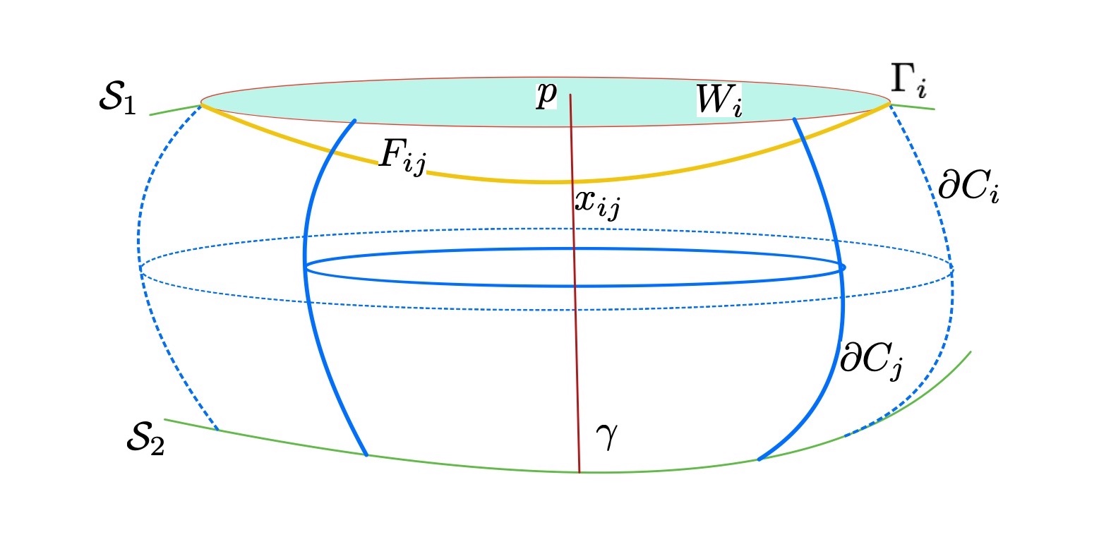
Figure 1: Construction of $F_{ij}$

We now wish to show the curvature of $F_{ij}$ is bounded independently of $i$ and to prove this we will show they have good area bounds to which the curvature estimates of Schoen-Simon-Yau [50, 52] apply. Cover $C_{j}$ by small balls $\mathcal{B}_{x_{k}}(2\delta)$ such that the balls $\mathcal{B}_{x_{k}}(\delta)$ already cover $C_{j}$. We choose $\delta$ sufficiently small so that each $\mathcal{B}_{x_{k}}(2\delta)$ is strictly convex and diffeomorphic to a unit ball of $\hbox{\bb R}^{n}$. We will use the topology of $\mathcal{B}_{x_{k}}(2\delta)$ to know a closed embedded piecewise smooth hypersurface in $\mathcal{B}_{x_{k}}(2\delta)$ bounds a domain in $\mathcal{B}_{x_{k}}(2\delta)$. $C_{j}$ is compact and $\mathcal{N}$ has bounded geometry so a finite number of $\mathcal{B}_{x_{k}}(\delta)$ suffice to cover $C_{j}$ and their number depends on the volume of $C_{j}$ and curvature bounds of $\tilde{\mathcal{N}}$. The balls are sufficiently small so the volume of their boundaries is at most $c\delta^{n-1}$ for some constant $c$ independent of $i$. For later use, we will cover $\mathcal{N}$ by a countable number of such small balls.

Claim A: The volume of $F_{ij}$ in each ball $\mathcal{B}_{x_{k}}(2\delta)$ is bounded by half the volume of $\partial\mathcal{B}_{x_{k}}(2\delta)$.

Proof of Claim A.

This statement can be found in [10, Example 8.9] however, we prefer to include it for the reader’s convenience.

We will suppose first $\mathcal{B}_{x_{k}}(2\delta)\equiv\mathcal{B}$ is the unit ball of $\hbox{\bb R}^{3}$ and $F_{ij}\cap\mathcal{B}=S_{1}\cup\ldots S_{m}$ are pairwise disjoint embedded surfaces, each $S_{l}$ meeting $\partial\mathcal{B}$ transversally in a finite number of (topological) circles. The reader can easily check the proof works as well with $\mathcal{B}$ replaced by $\mathcal{B}_{x_{k}}(2\delta)$ and the $S_{l}\mbox{}^{\prime}s$ replaced by the connected components of $F_{ij}\cap\mathcal{B}_{x_{k}}(2\delta)$, each connected component meeting $\partial\mathcal{B}_{x_{k}}(2\delta)$ transversally in pairwise disjoint closed embedded hypersurfaces in $\mathcal{B}_{x_{k}}(2\delta)$ (playing the role of the circles).

Let $S:=S_{1}\cup\ldots S_{m}$ and let $\beta_{1},\ldots,\beta_{r}$ be the pairwise disjoint circles of $S\cap\partial\mathcal{B}$. The complementary components of these circles in $\partial\mathcal{B}$ can be painted with two colors, which we will denote by ${\color[rgb]{1,0,0}\blacksquare}$ and ${\color[rgb]{0,0,1}\blacklozenge}$. So if $D$ is one such component labeled ${\color[rgb]{1,0,0}\blacksquare}$ say, then each circle in $\partial D$ is two-sided, with the label ${\color[rgb]{1,0,0}\blacksquare}$ on the $D$ side, and the label ${\color[rgb]{0,0,1}\blacklozenge}$ on the other side (a closed embedded hypersurface of $\partial\mathcal{B}_{x_{k}}(2\delta)$ separates it into two components and is orientable). Now label one component ${\color[rgb]{1,0,0}\blacksquare}$, then label the components of the other side of each circle in its boundary by ${\color[rgb]{0,0,1}\blacklozenge}$, and continue labeling until each component is assigned a ${\color[rgb]{1,0,0}\blacksquare}$ or ${\color[rgb]{0,0,1}\blacklozenge}$. So each circle is labeled ${\color[rgb]{1,0,0}\blacksquare}$ on one side and ${\color[rgb]{0,0,1}\blacklozenge}$ on the other side.

The reader can convince himself that this labeling works as follows. Choose some circle $\beta_{1}$ that bounds a domain $D_{1}$ on $\partial\mathcal{B}$ that contains no other circle. Label $D_{1}$ by ${\color[rgb]{1,0,0}\blacksquare}$. Let $D_{2}$ be the connected component of $\partial\mathcal{B}\setminus\left(D_{1}\cup\beta_{2}\cup\ldots\cup\beta_{r}\right)$ containing $\beta_{1}$ in its boundary and let $\beta_{2},\ldots,\beta_{\bar{r}}$, $\bar{r}\leq r$ and (relabeling if necessary) the remaining circles of $\partial D_{2}$. Label $D_{2}$ by ${\color[rgb]{0,0,1}\blacklozenge}$. Each $\beta_{2},\ldots,\beta_{\bar{r}}$ bounds a disk in $\partial\mathcal{B}\setminus D_{1}$, they are pairwise disjoint, and we continue the labeling in each disk bounded by the $\beta_{2},\ldots,\beta_{\bar{r}}$. So the labeling is an increasing sequence of domains of $\partial\mathcal{B}$ and terminates after a finite number of steps.

Now, $S$ is a disjoint union of the $S_{1},\ldots,S_{l}$. We attach the ${\color[rgb]{1,0,0}\blacksquare}$ domains $D_{\alpha}$ of $\partial\mathcal{B}$ to $S$ by gluing each circle in $\partial D_{\alpha}$ to the circle from which it came in $S$; i.e., in $\partial S_{\alpha}$ for some $S_{\alpha}$. This gives a finite number of piecewise smooth closed embedded surfaces $M_{1},\ldots,M_{r^{\prime}}$, $r^{\prime}\leq r$, in $\mathcal{B}$; smooth except along the circles. Each $M_{\nu}$ bounds a compact domain in $\mathcal{B}$ and the domains are pairwise disjoint. Each $M_{\nu}\cap{\rm int}(\mathcal{B})$ is homologous ${\rm mod}(2)$ to the ${\color[rgb]{1,0,0}\blacksquare}$ domains in $\partial M_{\nu}$.

Since $S$ is area-minimizing ${\rm mod}(2)$, the area of $M_{\nu}\cap{\rm int}(\mathcal{B})$ is at most the area of the ${\color[rgb]{1,0,0}\blacksquare}$ or ${\color[rgb]{0,0,1}\blacklozenge}$ domains in $\partial M_{\nu}$. Thus, the area of $S$ is less than half the area of $\partial\mathcal{B}$, which proves Claim A. ∎

Then, we can assert:

Claim B: The curvature estimates of Schoen-Simon-Yau [50, 52] apply, i.e., $F_{ij}$ has bounded curvature independent of $i$.

Proof of Claim B.

Since $C_{j}$ is covered by a finite number of small balls $\mathcal{B}_{x_{k}}(2\delta)$, with $\mathcal{B}_{x_{k}}(\delta)$ already covering $C_{j}$, and in each such ball $\mathcal{H}^{n-1}\left(F_{ij}\cap\mathcal{B}_{x_{k}}(2\delta)\right)\leq c\delta^{n-1}$, where $c$ depends on geometry of the ball and $c$ is the same for all $\delta$ sufficiently small. In fact, the bounded geometry of $\mathcal{N}$ will give the same estimate in each of the countable $\mathcal{B}_{x_{k}}(2\delta)$ of the covering of $\mathcal{N}$ for any properly embedded area-minimizing hypersurface ${\rm mod}(2)$ in $\mathcal{N}$ by Claim B. Thus, for any such hypersurface $\mathcal{F}$ one has (cf. [50, 52])

$${\rm sup}_{\mathcal{F}\cap\mathcal{B}_{x_{k}}(\delta)}|A_{\mathcal{F}}|^{2}\leq C(n,c)\delta^{-2},$$

for some constant $C(n.c)$ that only depends on the dimension $n\leq 7$ and $c$ above, $c$ depends on the bounds of the geometry of $\mathcal{N}$. Therefore, $F_{ij}$ has bounded curvature independent of $i$ greater than $j$ and Claim B is proved. ∎

The $F_{ij}$ have bounded curvature by Claim B thus (locally) they are graphs of bounded geometry over some $\tau$ ball in their tangent hyperplane at each point and $\tau$ only depends on curvature bounds. More precisely, the intrinsic ball of radius $\tau$ of $p\in F_{ij}$, $\mathcal{D}^{ij}_{p}(\tau)$, is the graph (in normal geodesic coordinates) of a function $u^{ij}_{p}$ defined on ${\rm exp}(D^{ij}_{p})$, $D^{ij}_{p}\subset T_{p}F_{ij}$ an open set of the tangent space centered at the origin ${\bf 0}\in T_{p}F_{ij}$, such that

$$u^{ij}_{p}({\bf 0})=0=|\nabla u^{ij}_{p}({\bf 0})|$$

and

$$|\nabla u^{ij}_{p}(y)|^{2}\leq\Lambda\tau^{2}\text{ and }|\nabla^{2}u^{ij}_{p}(y)|^{2}\leq\Lambda\tau^{2}\text{ for all }y\in D^{ij}_{p};$$

which implies that $\partial\mathcal{D}^{ij}_{p}(\tau)\cap\mathcal{B}_{p}(\tau/2)=\emptyset$. Since $\partial\mathcal{D}^{ij}_{p}(\tau)\cap\mathcal{B}_{p}(\tau/2)=\emptyset$, monotonicity of the area ratios gives a strictly positive lower bound for the area for all these local graphs $\mathcal{D}^{ij}_{p}(\tau)$ for all $p\in F_{ij}$ and $i>j$.

An important remark is that if $q\in F_{ij}\setminus\mathcal{D}^{ij}_{p}(2\tau)$, then $q$ can not be too close (in the extrinsic distance) to $p$. For when $q$ is close to $p$, $\mathcal{D}^{ij}_{p}(\tau)$ and $\mathcal{D}^{ij}_{q}(\tau)$ are disjoint since $F_{ij}$ is embedded. Then, by compacity of minimal graphs, $\mathcal{D}^{ij}_{p}(\tau/2)$ and $\mathcal{D}^{ij}_{q}(\tau/2)$, if $p$ and $q$ are sufficiently close, are graphs over the same domain ${\rm exp}(U_{p})$, $U_{p}\subset T_{p}F_{ij}$, that are $C^{2}-$close. Also $\partial\mathcal{D}^{ij}_{p}(\tau/2)$ and $\partial\mathcal{D}^{ij}_{q}(\tau/2)$ are $C^{2}-$close and they are the boundary of a (annular) hypersurface $\mathcal{A}$ of small volume. Replace $F_{ij}$ by removing $\mathcal{D}^{ij}_{p}(\tau/2)\cup\mathcal{D}^{ij}_{q}(\tau/2)$ and adding $\mathcal{A}$. This is congruent to $F_{ij}\,{\rm mod}(2)$ and of less volume if $q$ is sufficiently close to $p$. This is impossible since $F_{ij}$ is area-minimizing ${\rm mod}(2)$.

Now, $F_{ij}$ has finite volume independent of $i$ so can be covered by a finite number of the $\mathcal{D}^{ij}_{p}(\tau)$, $\mathcal{D}^{ij}_{p}(\tau)\subset F_{ij}$ is the graph (in normal geodesic coordinates) of a function $u^{ij}_{p}$ defined on an open set of the tangent space $D^{ij}_{p}\subset T_{p}F_{ij}$ centered at the origin ${\bf 0}\in T_{p}F_{ij}$ of bounded geometry controlled by $\tau$. Thus, each $F_{ij}$, for $j<i$, has an embedded tubular neighborhood of some fixed size independent of $i$, the size of the intrinsic graph neighborhood depends on the curvature estimate and area estimates.

Next we construct a limit $\mathcal{F}_{j}$ of a subsequence of $F_{ij}$ which will be an oriented embedded area-minimizing ${\rm mod}(2)$ hypersurface and $\mathcal{F}_{j}\cap\gamma\neq\emptyset$. Let $i\to\infty$ and choose a subsequence of the $x_{ij}$ that converges to a point $x_{j}\in\gamma$ and also their tangent hyperplanes at the points of the subsequence converge to a hyperplane $P_{j}\subset T_{x_{j}}\mathcal{N}$. The $\tau-$graphs $\mathcal{D}_{x_{ij}}(\tau)\subset F_{ij}$ of the subsequence converge to a minimal $(\tau/2)-$graph $\mathcal{G}_{j}$ (in normal geodesic coordinates over $P_{j}$) at $x_{j}$.

Since the tubular neighborhoods of the $F_{ij}$ have a fixed size, and the $x_{ij}$ are the highest points of intersection of $F_{ij}$ with $\gamma$, the convergence of the $\mathcal{D}_{x_{ij}}(\tau)$ to $\mathcal{G}_{j}$ is multiplicity one. So the normal of $F_{ij}$ at $x_{ij}$ pointing up, defines an orientation of the limit surface $\mathcal{G}_{j}$. Recall that $F_{i}$ and $W_{i}$ are homologous, they bound a domain $\Omega_{i}$. Along the converging subsequence (also called $F_{ij}$), the normal points into $\Omega_{i}$. The sequence converges $C^{2}$ to $\mathcal{F}_{j}$ ($\mathcal{F}_{j}$ compact) so $\mathcal{F}_{j}$ together with a compact domain on $\partial C_{j}$ is homologous to $C_{j}\cap\mathcal{S}_{1}$.

Each point of $\partial\mathcal{G}_{j}$ is also a limit of points in the graphs $\mathcal{D}_{x_{ij}}(\tau)$ and the normals converge to the normal at the boundary point of $\mathcal{G}_{j}$. The same limiting process at the boundary points of $\mathcal{G}_{j}$ extends $\tau/2$ further from its boundary. Continuing this by extending the boundary, we obtain an embedded minimal hypersurface $\mathcal{F}_{j}$ (with boundary) in $C_{j}$; which is a limit of the components of the $F_{ij}$ of the subsequence in $C_{j}$ as $i\to\infty$; let us explain such construction in more detail (cf. [37, Lemma 1.1] for a detailed proof in dimension three).

What follows is a standard way to get a convergent subsequence. Cover each $F_{ij}$ by a maximal number of pairwise disjoint local graphs $\mathcal{D}^{ij}_{p_{k}}(\tau/5)$, $k=1,\ldots,\nu$, $\nu$ is bounded by monotonicity and the uniform area bound of the $F_{ij}$ independently of $i$. We can suppose $\nu$ is fixed. Choose points $y_{ki}\in\mathcal{D}^{ij}_{p_{k}}(\tau/5)$ such that, up to subsequence, $y_{ki}\to y_{k}$ and the tangent hyperplanes of $\mathcal{D}^{ij}_{p_{k}}(\tau/5)$ at $y_{ki}$ converge to a hyperplane $P_{k}\subset T_{y_{k}}\mathcal{N}$, $k=1,\ldots,\nu$. Then, the minimal graphs $\mathcal{G}_{ki}(\tau/5):=\mathcal{D}^{ij}_{y_{ki}}(\tau/5)$ converge to minimal hypersurfaces $M^{\prime}_{1},\ldots M^{\prime}_{\nu}$ as $i\to\infty$, recall that $j$ is fixed.

By Vitali’s Covering Lemma, there exists a maximal pairwise disjoint subcollection $\mathcal{D}^{ij}_{y_{ki}}(\tau/5)$, $k=1,\ldots,\alpha\leq\nu$ up to re-ordering, such that

$$F_{ij}\subset\bigcup_{k=1}^{\alpha}\mathcal{D}^{ij}_{y_{ki}}(\tau)$$

and each $\mathcal{D}^{ij}_{y_{ki}}(\tau)$ converges to a minimal hypersurface $M_{k}$, $k=1,\ldots,\alpha$, as $i\to\infty$, recall that $j$ is fixed. Hence the limit hypersurface of these subsequences exists in $C_{j}$ if

$$\mathcal{F}_{j}=\bigcup_{k=1}^{\alpha}M_{k}$$

is a smooth embedded hypersurface.

Each $M_{k}$, $k=1,\ldots,\alpha$, is embedded since $F_{ij}$ is embedded. So it suffices to show if $M_{a}\cap M_{b}\neq\emptyset$, $a\neq b$, then $M_{a}=M_{b}$. If $M_{a}$ touches $M_{b}$ at a point (at one side) then $M_{a}=M_{b}$ by the Maximum Principle. Otherwise $M_{a}$ is transverse to $M_{b}$. Since

$$M_{a}:=\lim_{i\to\infty}\mathcal{D}^{ij}_{y_{ai}}(\tau)\text{ and }M_{b}:=\lim_{i\to\infty}\mathcal{D}^{ij}_{y_{bi}}(\tau),$$

for $i$ large, $\mathcal{D}^{ij}_{y_{ai}}(\tau)\cap\mathcal{D}^{ij}_{y_{bi}}(\tau)\neq\emptyset$ and meet transversally; this contradicts $F_{ij}$ is embedded. Thus, $\mathcal{F}_{j}$ is the desired limit.

Notice that when $M_{a}=M_{b}$, $a\neq b$, the convergence to $\mathcal{F}_{j}$ is with multiplicity greater than $1$ and less or equals to $\alpha$. Since $F_{ij}$ is area-minimizing ${\rm mod}(2)$, we know the multiplicity is one, i.e., two local graphs can not be disjoint and uniformly close to each other since one could reduce the area by a cut and paste argument. Moreover, $\mathcal{F}_{j}$ is oriented since there is only one local graph of $F_{ij}$ converging to $\mathcal{F}_{j}$ ($F_{ij}$ has an embedded tubular neighborhood of fixed size), and $\mathcal{F}_{j}\cap\gamma\neq\emptyset$.

Now repeat this process starting with the above subsequence of the $F_{i}\mbox{}^{\prime}s$ and look at the components intersecting $C_{2j}$ (so $i>2j$) that equal the components in $C_{j}$ we made limit to $P_{j}\subset T_{x_{j}}\mathcal{N}$. A subsequence of this family converges to a limit $\mathcal{F}_{2j}$ that equals $\mathcal{F}_{j}$ in $C_{j}$; we have the same local area and curvature estimates in the balls $\mathcal{B}_{x_{k}}(2\delta)$ covering $C_{2j}$. Then, letting $j\to\infty$, we obtain the complete, embedded, orientable, area-minimizing ${\rm mod}(2)$ hypersurface $\mathcal{F}$. Moreover, $\mathcal{F}$ is homologous to $\mathcal{S}_{1}$ since $\mathcal{F}\cap C_{j}$ together with a compact domain on $\partial C_{j}$ is homologous to $C_{j}\cap\mathcal{S}_{1}$ for all $j\in\hbox{\bb N}$. When $j$ goes to infinity, the limit $\mathcal{F}$ is homologous to $\mathcal{S}_{1}$.

∎

We showed above that if $q\in F_{ij}\setminus\mathcal{D}_{p}(2\tau)$, then $q$ can not be too close (in the extrinsic distance) to $p$. This argument also proves:

Theorem 3.2 (Tubular Neighborhood Theorem for ${\rm mod}(2)-$minimizers).

Let $(\mathcal{M}^{n},g)$, $3\leq n\leq 7$, be a complete, orientable manifold of bounded geometry. If $\mathcal{F}\subset\mathcal{M}$ is a complete, orientable, embedded hypersurface that is area-minimizing ${\rm mod}(2)$, then $\mathcal{F}$ is proper. Moreover, there exists $\epsilon>0$ (depending only on the bounds for the sectional curvatures and the second fundamental form) such that ${\rm Tub}_{\epsilon}(\mathcal{F})$ is embedded.

Proof.

By Claims A and B in Lemma 3.1, $\mathcal{F}$ has bounded second fundamental form. Hence, there exists $\tau>0$ (depending on the curvature bounds) such that the intrinsic ball of radius $\tau$ of $p\in F$, $\mathcal{D}_{p}(\tau)$, is the graph (in normal geodesic coordinates) of a function $u_{p}$ defined on ${\rm exp}(D_{p})$, $D_{p}\subset T_{p}\mathcal{F}$ an open set of the tangent space centered at the origin ${\bf 0}\in T_{p}\mathcal{F}$, such that $\partial\mathcal{D}_{p}(\tau)\cap\mathcal{B}_{p}(\tau/2)=\emptyset$. The result will be proven if we show:

Claim A: There exists $\epsilon>0$ (depending on $\tau$) such that for any two points $p,q\in\mathcal{F}$ with ${\rm dist}_{\mathcal{F}}(p,q)>2\tau$, then ${\rm dist}_{\mathcal{M}}(p,q)>\epsilon$.

Proof of Claim A.

By contradiction, assume there exists $p\in\mathcal{F}$ and a sequence $\left\{p_{n}\right\}_{n\in\hbox{\bbp N}}\subset\mathcal{F}$ such that ${\rm dist}_{\mathcal{F}}(p,p_{n})>2\tau$ and ${\rm dist}_{\mathcal{M}}(p,p_{n})<1/n$. By compacity of minimal graphs, $\mathcal{D}_{p_{n}}(\tau/2)$ and $\mathcal{D}_{p}(\tau/2)$ are graphs over the same domain ${\rm exp}(U_{p})$, $U_{p}\subset T_{p}F$ for $n$ large enough, that are $C^{2}-$close. Also $\mathcal{D}_{p_{n}}(\tau/2)\cap\mathcal{B}_{p}(\tau/4)$ and $\mathcal{D}_{p}(\tau/2)\cap\mathcal{B}_{p}(\tau/4)$ are $C^{2}-$close and they are the boundary of a (annular) hypersurface $\mathcal{A}\subset\partial\mathcal{B}_{p}(\tau/4)$ of small volume. Replace $\mathcal{F}$ by removing $\left(\mathcal{D}^{ij}_{p}(\tau/2)\cup\mathcal{D}^{ij}_{q}(\tau/2)\right)\cap\mathcal{B}_{p}(\tau/4)$ and adding $\mathcal{A}$. This is congruent to $\mathcal{F}\,{\rm mod}(2)$ and of less volume if $p_{n}$ is sufficiently close to $p$. This is impossible since $\mathcal{F}$ is area-minimizing ${\rm mod}(2)$. This proves Claim A. ∎

Then, Claim A above proves the theorem. ∎

Now, we can outline the proof of:

Theorem $\tilde{{\rm\bf A}}$: Let $\mathcal{M}^{n}$ , $3\leq n\leq 7$, be a complete manifold of bounded geometry. Suppose $\Sigma^{n-1}\subset\mathcal{M}^{n}$ is a two-sided properly embedded minimal hypersurface that has an $\epsilon-$tubular neighborhood ${\rm Tub}_{\epsilon}(\Sigma)$ that is embedded, well-oriented and of bounded extrinsic geometry. If $\Sigma$ is parabolic then the Maximum Principle at Infinity holds for $\Sigma$; i.e., if $S$ is a proper minimal hypersurface so that $\Sigma\cap S=\emptyset$ and $S\cap{\rm Tub}_{\epsilon}(\Sigma)\neq\emptyset$, then $S$ is an equidistant of $\Sigma$.

The Theorem A of L. Mazet is valid in dimensions $3\leq n\leq 7$ for constant mean curvature hypersurfaces exactly as he stated. The proof is simpler for minimal hypersurfaces; there are fewer terms in the calculations and inequalities to verify, but the idea of the proof is the same. We suggest an interested reader study his proof for minimal surfaces first.

We remark on a small change in the proof of Mazet in dimension $n>3$. Let $S$ be the properly immersed minimal hypersurface entering the $\epsilon-$tubular neighborhood of the parabolic minimal hypersurface $\Sigma$. Mazet begins by explaining that if $S$ is stable his proof will proceed in a manner he will consider later. So, he first discusses his proof when $S$ is not stable.

The proof he then gives, when $S$ is not stable, yields a stable $S^{\prime}$ to work with in the place of the original $S$. Then he proceeds the proof with this new $S^{\prime}$. The important property used of $S^{\prime}$ is the curvature estimates for stable minimal surfaces in dimension three: they only depend on the bounded ambient geometry and the distance to the boundary, not on local area bounds. In higher dimensions such curvature estimates are known when one has local area bounds; e.e., as we described in Lemma 3.1 for area minimizers in homology classes ${\rm mod}(2)$.

The stable $S^{\prime}$ Mazet obtains does have local area bounds and is smoothly embedded. He considers certain open sets in a compact region with rectifiable boundaries and minimizes the area functional of their boundaries. Geometric Measure Theory gives the existence and regularity of a minimizer and thus one has local area estimates for this type of minimizer, as we did in Lemma 3.1. Hence, one has curvature estimates (bounded curvature) at points at fixed positive distance from $\partial S^{\prime}$. Mazet then proceeds with his proof using this $S^{\prime}$

Now the proof to obtain $S^{\prime}$ began assuming $S$ was unstable; he then foliated a neighborhood of $S$ by constant mean curvature surfaces whose mean curvature vectors pointed away from $S$ (all this in a compact ambient domain).

For us, we must explain what to do in higher dimensions if the $S$ one started with was stable; $S$ may not have local area bounds. Here, we use a trick discovered by A. Song [55, Lemma 17].

Let $p\in S$ be a point where a neighborhood of $S$ is embedded. There is a small extrinsic ball $\mathcal{B}_{p}(\delta)$ of $\Sigma\times[0,\epsilon]$, centered at $p$ of radius $\delta>0$ small, and a smooth Riemannian metric on $\Sigma\times[0,\epsilon]$ equal to the original metric on the complement of $\mathcal{B}$ and there is a minimal unstable hypersurface $\tilde{S}$ with $\partial\tilde{S}=\partial S$ in the compact cylinder $K_{n}\times[0,\epsilon]$; $K_{n}$ a compact of $\Sigma$.

Finally, proceed with Mazet’s proof with this unstable $\tilde{S}$.

4 Embedded $\epsilon-$tube

Let $\Sigma^{n-1}\subset\mathcal{M}^{n}$ be a proper two-sided embedded hypersurface. Define the map $F:\Sigma\times\hbox{\bb R}\to\mathcal{M}$ given by

$$F(p,t):={\rm exp}_{p}(tN(p))$$ (4.1)

and, since $\Sigma$ is at least $C^{2}$, there exists a tubular neighborhood $\Omega$ of $\Sigma$ in $\mathcal{M}$ formed by non-intersecting, minimal geodesics starting normally from $\Sigma$. Hence, by possible choosing a smaller tubular neighborhood that we still denote by $\Omega$, the map $F^{-1}$ is well-defined and smooth in $\Omega\setminus\Sigma$ and there exists an open subset $\Lambda\subset\Sigma\times\left(\hbox{\bb R}\setminus\left\{0\right\}\right)$ with the property that if $(p,t)\in\Lambda$ then also $(p,s)\in\Lambda$ for all $0<|s|<|t|$. Hence, the map $F_{|\Lambda}:\Lambda\to\Omega\setminus\Sigma$ is a diffeomorphism and for every point $p\in\Omega$ there exists a unique point of minimum distance to $\Sigma$; that is, $\Omega$ has the unique projection property (see [2, 4]). Let $\left\{K_{i}\right\}_{i\in\mathbb{N}}$ be a compact exhaustion of $\Sigma$ so that $K_{i}\subset K_{i+1}$ and define

$$\epsilon_{i}:={\rm inf}_{K_{i}}{\rm sup}\left\{t>0\,:\,\,(p,s)\in\Lambda\text{ for all }0<|s|<t\text{ and }p\in K_{i}\right\}.$$ (4.2)

Observe that if $\epsilon:={\rm inf}\left\{\epsilon_{i}>0\,:\,\,i\in\hbox{\bb N}\right\}>0$, the above construction gives an embedded $\epsilon-$tube. The existence of an embedded $\epsilon-$tube is crucial when we want to apply Maximum Principles at Infinity. In this sense, following ideas of [39, 45], we can assert:

Theorem 4.1 (Tubular Neighborhood Theorem).

Let $(\mathcal{M}^{n},g)$, $3\leq n\leq 7$, be a complete manifold of bounded geometry and $\overline{Ric}\geq 0$. Let $\Sigma\subset\mathcal{M}$ be a properly embedded, two-sided, parabolic, minimal hypersurface of bounded second fundamental form. Then, there exists $\epsilon>0$ (depending only on the bounds for the sectional curvatures and the second fundamental form) such that ${\rm Tub}_{\epsilon}(\Sigma)$ is embedded. Moreover, ${\rm Tub}_{\epsilon}(\Sigma)$ is well-oriented and of bounded extrinsic geometry (cf. Definition 1.1).

Remark 4.1.

An ideal triangle in the hyperbolic plane shows the hypothesis Ricci non negative is necessary.

Proof of Theorem 4.1.

Since there exists a constant $C>0$ so that ${\rm inj}(\mathcal{M})\geq 1/C$, $\left|\overline{K}_{ij}\right|\leq C$ and $\left|A\right|\leq C$; there exists $\delta^{\prime}>0$ (depending only on $C$) such that the map $F:\Sigma\times(-\delta^{\prime},\delta^{\prime})\to\mathcal{M}$, given by (4.1), is smooth and for each $p\in\Sigma$, $F:D_{p}(\delta^{\prime})\times(-\delta^{\prime},\delta^{\prime})\to\mathcal{M}$ is injective. Also, $F^{*}g$ denotes the pullback metric on $\Sigma\times(-\delta,\delta)$ induced by the map $F:\Sigma\times(-\delta^{\prime},\delta^{\prime})\to(\mathcal{M},g)$.

Observe that $(\Sigma\times[-\delta,\delta],F^{*}g)$, for any $\delta\in(0,\delta^{\prime})$, defines an embedded $\delta-$tube for $\Sigma(0)\equiv\Sigma\times\left\{0\right\}$. Moreover, by the First Variation Formula for the Mean Curvature (2.6) and the fact that the Ricci curvature is non-negative, the mean curvature of $\Sigma(t)=\Sigma\times\left\{t\right\}$ satisfies $H^{\prime}(t)\geq 0$ for all $t\in(-\delta,\delta)$; this implies that $(\Sigma\times[-\delta,\delta],F^{*}g)$ is well-oriented. Also, by [27, pages 179-180] and the fact that the geometry of $\mathcal{M}$ and $\Sigma$ are bounded by $C$ above; all the equidistants $\Sigma(t)$ have bounded second fundamental form and are quasi-isometric to $\Sigma$ (depending on $C$ and $\delta$). That is, $(\Sigma\times[-\delta,\delta],F^{*}g)$ has bounded extrinsic geometry (cf. Definition 1.1). Now, $\Sigma(0)\subset F^{-1}(\Sigma)$ and $F_{|\Sigma(0)}$ is injective.

Claim A: If there are componentes of $F^{-1}(\Sigma)$ other than $\Sigma_{0}$, then $\mathcal{M}$ is a mapping torus over $\Sigma$; i.e., there exists $\tau>0$ such that $\mathcal{M}$ is isometric to $\Sigma\times[0,\tau]$, with the product metric, where $\Sigma\times\left\{0\right\}$ is identified with $\Sigma\times\left\{\tau\right\}$ by an isometry. In this case, ${\rm Tub}_{\epsilon}(\Sigma)$ is embedded, well-oriented and of bounded extrinsic geometry (cf. Definition 1.1) for any $\epsilon<\tau/2$.

Proof of Claim A.

Let $E\subset F^{-1}(\Sigma)\setminus\Sigma_{0}$ be such a component, $E$ is a proper minimal hypersurface in $(\Sigma\times[-\delta,\delta],F^{*}g)$ disjoint from $\Sigma\times\left\{0\right\}$. Since $\Sigma$ is proper, for some $p\in\Sigma$, we can suppose $E$ is the highest component of $F^{-1}\left(\Sigma\right)\setminus\Sigma_{0}$ below $\Sigma_{0}$ (cf. Figure 1).

By Theorem ${\rm\tilde{A}}$, such a component $E\subset F^{-1}(\Sigma)$ is an equidistant of $\Sigma(0)$; so $E=\Sigma(\tau)$ for some $\tau\in(0,\delta)$. Thus, by the First Variation Formula of the Mean Curvature (2.6), $\Sigma(t)\subset(\Sigma\times[-\delta,\delta],F^{*}g)$ is totally geodesic for each $t\in[0,\tau]$. By Lemma 7.1, the metric on $\Sigma\times[0,\tau]$ is a product metric $F^{*}g=\sigma+dt^{2}$.

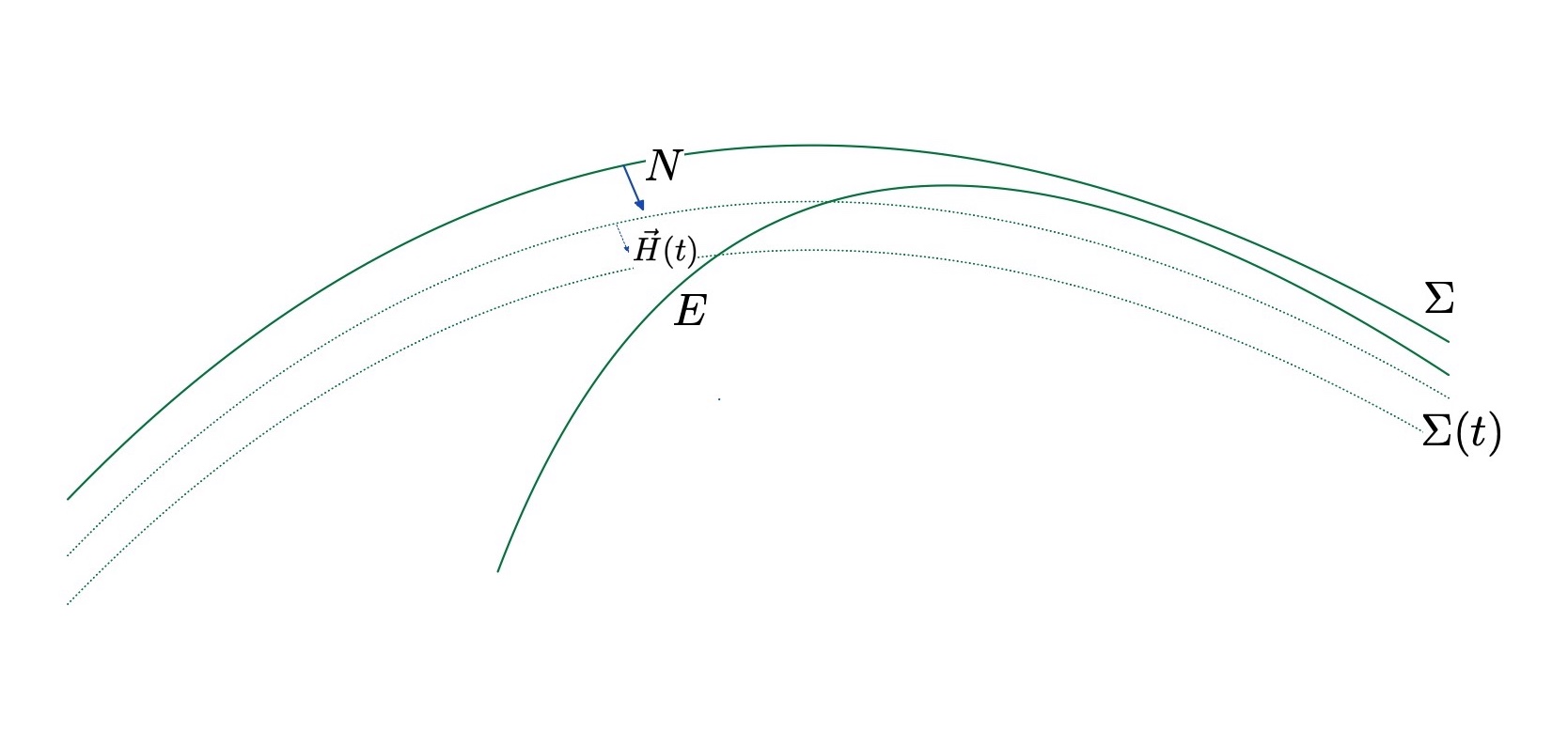
Figure 2: $E$ is a proper minimal hypersurface in $(\Sigma\times[-\delta,\delta],F^{*}g)$

Moreover, $F(\Sigma(0))=\Sigma=F(\Sigma(\tau))$ and, hence, $F(\Sigma\times[0,\tau])$ is open and closed in $\mathcal{M}$, which means that $\mathcal{M}$ is a torus manifold over $\Sigma$. ∎

So suppose from now on that $F^{-1}(\Sigma)=\Sigma_{0}$. Let $0<\tau<\delta$ and assume $F:\Sigma\times(-\tau,\tau)\to\mathcal{M}$ is not an embedding. We will show this gives a contradiction if $\tau$ is sufficiently small.

Let $z_{1},z_{2}\in\Sigma\times(-\tau,\tau)$, $F(z_{1})=F(z_{2})$, $z_{1}\neq z_{2}$. We have $z_{k}=(x_{k},t_{k})$, $k=1,2$, with $|t_{k}|<\tau$. Since $F:D_{p}(\delta)\times(-\tau,\tau)\to\mathcal{M}$ is injective for all $p\in\Sigma$, we have $x_{i}\not\in D_{x_{j}}(\delta)$ for $i\neq j$. Also,

$$\begin{split}{\rm dist}_{\mathcal{M}}(F(x_{1},0),F(x_{2},0))&\leq{\rm dist}_{\mathcal{M}}(F(x_{1},0),F(z_{1}))+{\rm dist}_{\mathcal{M}}(F(z_{1}),F(x_{2},0))\\[5.69054pt] &={\rm dist}_{\mathcal{M}}(F(x_{1},0),F(z_{1}))+{\rm dist}_{\mathcal{M}}(F(z_{2}),F(x_{2},0))\\[5.69054pt] &=|t_{1}|+|t_{2}|\leq 2\tau.\end{split}$$ (4.3)

Now, $\bar{F}:=F_{|B_{x_{1}}(\delta)\times(-\delta,\delta)}$ is an isometry onto an open neighborhood $\mathcal{U}\subset\mathcal{M}$ of $x_{1}$. Choose a large integer $k\in\hbox{\bb N}$ so that for $\tau=\delta/k$, the geodesic ball of $\mathcal{M}$ centered at the point $x_{1}=F(x_{1},0)\in\mathcal{M}$ of radius $2\tau>0$, $\mathcal{B}_{x_{1}}(2\tau)$, is contained in $\mathcal{U}$. So, $x_{2}=F(x_{2},0)\in\mathcal{B}_{x_{1}}(2\tau)\cap\Sigma$ by (4.3). The point $y:=\bar{F}^{-1}(F(x_{2},0))$ is in $D_{x_{1}}(\delta)\times(-\delta,\delta)$ and on a connected component of $F^{-1}(\Sigma)$ disjoint from $D_{x_{1}}(\delta)\times(-\delta,\delta)$. This is a contradiction.

∎

5 Splitting and non-separating hypersurfaces

We deal first with quasi-embedded non-separating hypersurfaces $\Sigma\subset\mathcal{M}$, loosely speaking, those that do not separate $\mathcal{M}$ into two components. When $\Sigma$ is embedded and compact, we can cut-open the manifold $\mathcal{M}$ through $\Sigma$ using a locally invertible map to obtain a new manifold with two boundary components, each one diffeomorphic to $\Sigma$, and in the interior isometric to $\mathcal{M}\setminus\Sigma$ (see [34] for details). We will extend this for properly embedded hypersurfaces, not necessarily compact.

Proposition 5.1.

Let $\Sigma^{n-1}\subset\mathcal{M}^{n}$ be a non-separating two-sided properly embedded hypersurface. There is a manifold $\mathcal{N}$ with two boundary components $\Sigma_{1}$ and $\Sigma_{2}$ and a locally invertible smooth map $\varphi:\mathcal{N}\to\mathcal{M}$ such that $\varphi:\mathcal{N}\setminus(\Sigma_{1}\cup\Sigma_{2})\to\mathcal{M}\setminus\Sigma$ is a diffeomorphism and $\varphi:\Sigma_{i}\to\Sigma$ is a diffeomorphism for $i=1,2$.

Proof.

Take any exhaustion $\left\{K_{i}\right\}_{i\in\mathbb{N}}\subset\Sigma$ and define $\epsilon_{i}>0$ given by (4.2). Now, we can construct a positive smooth function $f:\Sigma\to\hbox{\bb R}^{+}$ so that $2f(p)<\epsilon_{1}$ for all $p\in K_{1}$ and $2f(p)<\epsilon_{i}$ for all $p\in K_{i}\setminus K_{i-1}$ and $i\geq 2$. Then, define the open sets

$$\mathcal{U}^{\pm}:=\left\{F(p,t)\in\mathcal{M}:\,(p,t)\in\Lambda\text{ so that }0<\pm t<f(p)\right\}$$

then $\mathcal{U}^{\pm}\subset\Omega\setminus\Sigma$ and, up to shrinking if necessary, we can assume that $\mathcal{U}^{-}\cap\mathcal{U}^{+}=\emptyset$. Set $\mathcal{M}_{f}:=\mathcal{M}\setminus\left(\overline{\mathcal{U}^{-}\cup\mathcal{U}^{+}}\right)$ and consider the open sets

$$\Lambda^{\pm}:=\left\{(p,t)\in\Sigma\times\hbox{\bb R}^{\pm}\,:\,\,f(p)<\pm t<2f(p)\right\}$$

and

$$\tilde{\Lambda}^{\pm}:=\left\{(p,t)\in\Sigma\times\hbox{\bb R}\,:\,\,0\leq\pm t<f(p)\right\}$$

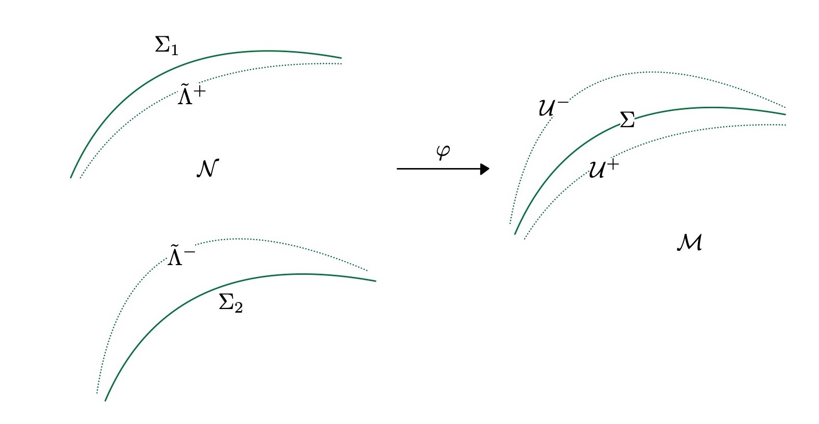
Figure 3: $\varphi:\mathcal{N}\setminus(\Sigma_{1}\cup\Sigma_{2})\to\mathcal{M}\setminus\Sigma$ is a diffeomorphism

Define $\mathcal{N}$ as the quotient of the disjoint union of $\mathcal{M}_{f}$, $\tilde{\Lambda}^{+}$ and $\tilde{\Lambda}^{-}$ by the identification $(p,t)\equiv F(p,t)\in\mathcal{M}_{f}$ for $(p,t)\in\Lambda^{\pm}$. The map $\varphi$ is the identity on $\mathcal{M}_{f}$ and $F$ on $\tilde{\Lambda}^{+}$ and $\tilde{\Lambda}^{-}$. $\Sigma_{1}$ and $\Sigma_{2}$ are the two copies of $\Sigma\times\left\{0\right\}$ (cf. Figure 3). ∎

Proposition 5.1 is a way to construct a new manifold with mean convex boundary. This is a good domain to construct (homologically) area-minimizing hypersurfaces. Thanks to the structure of stable hypersurfaces in manifolds of non-negative sectional curvature and scalar curvature bounded below that implies parabolicity [13], we can prove:

Theorem 5.1.

Let $(\mathcal{M}^{n},g)$, $n=4$, be a complete orientable manifold of bounded geometry, $\overline{K}_{ij}\geq 0$ and $\overline{Sc}\geq c>0$. Let $\Sigma\subset\mathcal{M}$ be a properly quasi-embedded, orientable, minimal hypersurface. Assume $\Sigma$ does not separate, then:

• $\Sigma$ is embedded.

• $\mathcal{M}^{4}$ is a mapping torus; i.e., $\mathcal{M}^{4}$ is isometric to $\Sigma\times[0,{\bf d}]$, with the product metric, where $\Sigma\times\left\{0\right\}$ is identified with $\Sigma\times\left\{{\bf d}\right\}$ by an isometry.

• If $\tilde{\Sigma}$ is an orientable, properly inmmersed minimal hypersurface in $\mathcal{M}\setminus\Sigma$, then $\tilde{\Sigma}=\Sigma\times\left\{t\right\}$ for some $t\in[0,{\bf d}]$.

Proof.

We will first prove the result assuming $\Sigma$ is embedded and stable.

Case 1: If $\Sigma$ is embedded and stable, then item ${\rm(ii)}$ and ${\rm(iii)}$ hold.

Proof of Case 1.

In this case, $\Sigma$ is totally geodesic and parabolic (cf. [13]). Hence, Theorem 4.1 implies that there exists $\epsilon>0$ so that ${\rm Tub}_{\epsilon}(\Sigma)$ is embedded, well-oriented and of bounded extrinsic geometry.

By Proposition 5.1, there is a manifold $\mathcal{N}$ with two boundary components $\Sigma_{1}$ and $\Sigma_{2}$ and a locally invertible smooth map $\varphi:\mathcal{N}\to\mathcal{M}$ such that $\varphi:\mathcal{N}\setminus(\Sigma_{1}\cup\Sigma_{2})\to\mathcal{M}\setminus\Sigma$ is a diffeomorphism and $\varphi:\Sigma_{k}\to\Sigma$ is a diffeomorphism for $k=1,2$. Since $\Sigma$ has an embedded $\epsilon-$tube, in the construction of $\varphi$ we can take $f\equiv\epsilon$. Consider the open sets

$$\Omega_{k}:=\left\{p\in\mathcal{N}\,:\quad d_{\mathcal{N}}(p,\Sigma_{k})<\epsilon\right\}\text{ for }k=1,2.$$

Fix $q_{1}\in\Sigma_{1}$, ${\bf d}:={\rm dist}_{\mathcal{N}}(q_{1},\Sigma_{2})$ and $\gamma:[0,{\bf d}]\to\mathcal{N}$ a minimizing geodesic such that $|\gamma|={\bf d}={\rm dist}_{\mathcal{N}}(q_{1},q_{2})$, $\gamma(0):=q_{2}\in\Sigma_{2}$, $\gamma$ is orthogonal to $\Sigma_{2}$ at $q_{2}$ and $\gamma([0,{\bf d}])\cap\left(\Sigma_{1}\cup\Sigma_{1}\right)=\left\{q_{1},q_{2}\right\}$.

Claim A: Either $\Omega_{1}\cap\Omega_{2}=\emptyset$ or $\mathcal{N}$ is isometric to the Riemannian product $\Sigma_{1}\times[0,{\bf d}]$.

Proof of Claim A.

Assume $\Omega_{1}\cap\Omega_{2}\neq\emptyset$. Set $\mathcal{S}_{k}=\partial\Omega_{k}\setminus\Sigma_{k}$, $k=1,2$, and assume $\mathcal{S}_{1}\cap\Omega_{2}\neq\emptyset$.

If some connected component of $\mathcal{S}_{1}\cap\Omega_{2}$ is compact, the Maximum Principle at the closest point to $\Sigma_{2}$ shows that $\mathcal{S}_{1}$ is an equidistant of $\Sigma_{2}$. Since the orientation of $\mathcal{S}_{1}\cap\Omega_{2}$ that makes the mean curvature non-negative points towards $\Sigma_{2}$ and the orientation of the equidistant to $\Sigma_{2}$ that makes the mean curvature non-negative points away from $\Sigma_{2}$ by (2.6); the only possibility is that $\mathcal{S}_{1}\cap\Omega_{2}$ is minimal. Hence, $\widetilde{\mathcal{S}}:=\mathcal{S}_{1}$ is minimal and equidistant of $\Sigma_{1}$ and $\Sigma_{2}$.

If all connected components of $\mathcal{S}_{1}\cap\Omega_{2}$ are non-compact. Then, reasoning as in Theorem ${\rm\tilde{A}}$, one shows there is a stable hypersurface $\mathcal{S}^{\prime}$ below $\mathcal{S}_{1}$ in $\Omega_{2}\setminus\Sigma_{2}$ such that $\partial\mathcal{S}^{\prime}\subset\Sigma_{2}(\epsilon^{\prime})$, $\epsilon^{\prime}<\epsilon/2$. This gives that the original $\widetilde{\mathcal{S}}:=\mathcal{S}_{1}\cap\Omega_{2}$ is an equidistant of $\Sigma_{2}$.

Thus, in any case, there exists a minimal hypersurface $\widetilde{\mathcal{S}}\subset\Omega_{1}\cap\Omega_{2}$ that is equidistant of $\Sigma_{1}$ and $\Sigma_{2}$. Hence, any point $p\in\mathcal{N}$ belongs either to $\widetilde{\mathcal{S}}$ or one of the the regions between $\widetilde{\mathcal{S}}$ and $\Sigma_{k}$ in $\Omega_{k}$ ($k=1,2$); that is, $\mathcal{N}=\Omega_{1}\cup\Omega_{2}$. Lemma 7.1 then implies that $\mathcal{N}$ is isometric to the Riemannian product $\Sigma_{1}\times[0,{\bf d}]$. Claim A is proved when $\Omega_{1}\cap\Omega_{2}\neq\emptyset$. ∎

Assume now that $\Omega_{1}\cap\Omega_{2}=\emptyset$. Consider the manifold with boundary $\widetilde{\mathcal{N}}=\mathcal{N}\setminus(\Omega_{1}\cup\Omega_{2})$, the boundary components denoted by $\mathcal{S}_{k}=\partial\Omega_{k}\setminus\Sigma_{k}$, $k=1,2$. Let $\tilde{\gamma}\subset\tilde{\mathcal{N}}$ be a geodesic segment of $\gamma$ joining a point $p_{1}\in\mathcal{S}_{1}$ to a point $p_{2}\in\mathcal{S}_{2}$; moreover, we know $|\tilde{\gamma}|\leq{\bf d}-\epsilon$. By Lemma 3.1, there is a two-sided properly embedded stable minimal hypersurface $\mathcal{F}_{1}\subset\tilde{\mathcal{N}}$ homologous to $\mathcal{S}_{1}$ and, by [13], $\mathcal{F}_{1}$ is parabolic. Denote by $\mathcal{N}_{1}$ the region of $\mathcal{N}$ between $\Sigma_{1}$ and $\mathcal{F}_{1}$.

If $\mathcal{F}_{1}$ touches $\mathcal{S}_{1}$ at a point $z$ at one side, then $\mathcal{F}_{1}=\mathcal{S}_{1}$ by the Maximum Principle; the mean curvature vector of $\mathcal{S}_{1}$ at $z$ points into $\tilde{\mathcal{N}}$. By the First Variation Formula for the Mean Curvature (2.6), the region of $\mathcal{N}_{1}\subset\mathcal{N}$ is foliated by totally geodesic hypersurfaces and Lemma 7.1 then says the region $\overline{\mathcal{N}_{1}}$ is isometric to the product manifold $\Sigma_{1}\times[0,\epsilon]$.

Recall that $\mathcal{S}_{1}=\Sigma_{1}(\epsilon)$ is the equidistant of $\Sigma_{1}$ at distance $\epsilon$. Theorem 4.1 implies that $\mathcal{F}_{1}$ has an embedded $\epsilon-$tube, observe that ${\rm Tub}_{\epsilon}(\mathcal{F}_{1})\subset\mathcal{N}$. Let $\mathcal{F}_{1}(\epsilon)$ denote the equidistant of $\mathcal{F}_{1}$ at distance $\epsilon$ that is in $\mathcal{N}_{1}$. If $\mathcal{F}_{1}(\epsilon)$ intersects $\Sigma_{1}(\epsilon)$ at a point $z$ then first observe that $\mathcal{F}_{1}(\epsilon)$ can not touch $\Sigma_{1}(\epsilon)$ at $z$ (locally on one side), since their mean curvature vectors would point in opposite directions at $z$ so $\mathcal{F}_{1}(\epsilon)=\Sigma_{1}(\epsilon)$. Then, by Lemma 7.1, $\mathcal{N}_{1}$ is a Riemannian product bounded by the parallel hypersurfaces $\Sigma_{1}$ and $\mathcal{F}_{1}$; which is what we want to prove.

So we can suppose $\mathcal{F}_{1}(\epsilon)$ traverses $\Sigma_{1}(\epsilon)$ locally near $z$. But then an equidistant of $\mathcal{F}_{1}$ has a component in ${\rm Tub}_{\epsilon}(\Sigma_{1})$. As we saw previously, this implies the component is also an equidistant of $\Sigma_{1}$, hence, again, $\mathcal{N}_{1}$ splits as a Riemannian product bounded by the parallel hypersurfaces $\Sigma_{1}$ and $\mathcal{F}_{1}$.

Now suppose ${\rm Tub}_{\epsilon}(\mathcal{F}_{1})\cap\overline{\Omega}_{1}=\emptyset$. Let $\tilde{\mathcal{N}}_{2}$ be the closure of $\mathcal{N}_{1}\setminus\left({\rm Tub}_{\epsilon}(\mathcal{F}_{1})\cup{\rm Tub}_{\epsilon}(\Sigma_{1})\right)$, $\tilde{\mathcal{N}}_{2}$ has boundary $\mathcal{F}_{1}(\epsilon)\cup\Sigma_{1}(\epsilon)$. Let $\tilde{\gamma}$ be the geodesic segment of $\gamma$ in the interior of $\tilde{\mathcal{N}}_{2}$, joining a point $z_{1}\in\mathcal{F}_{1}(\epsilon)$ to a point $x\in\Sigma_{1}(\epsilon)$.

Now we can construct a two-sided properly embedded stable minimal hypersurface $\mathcal{F}_{2}$ in $\tilde{\mathcal{N}}_{2}$, $\mathcal{F}_{2}$ homologous to $\Sigma_{1}(\epsilon)$, and $\mathcal{F}_{2}$ has non zero intersection number with $\tilde{\gamma}$. $\mathcal{F}_{2}$ is constructed in the same manner we constructed $\mathcal{F}_{1}$. The highest point of $\mathcal{F}_{2}\cap\tilde{\gamma}$, denoted by $z_{2}$, is at least $\epsilon$ higher than $z_{1}$, the highest point of $\mathcal{F}_{1}\cap\gamma$. Also, ${\rm dist}_{\mathcal{N}}(\mathcal{F}_{2},\Sigma_{1})\geq\epsilon$.

If ${\rm Tub}_{\epsilon}(\mathcal{F}_{2})\cap\Omega_{1}\neq\emptyset$, we conclude as before that the domain bounded by $\Sigma_{1}$ and $\mathcal{F}_{2}$ splits. If the intersection is empty, we construct a higher least area $\mathcal{F}_{3}$ in $\tilde{\mathcal{N}}_{3}$, the closure of $\tilde{\mathcal{N}}_{2}\setminus\left({\rm Tub}_{\epsilon}(\mathcal{F}_{2})\cup{\rm Tub}_{\epsilon}(\Sigma_{1})\right)$, and continue. After a finite number of steps, we must have ${\rm Tub}_{\epsilon}(\mathcal{F}_{k})\cap\Omega_{1}\neq\emptyset$. So, we can suppose $k=1$ and $\mathcal{N}_{1}$ is a product manifold over $\Sigma_{1}$.

Then, consider the manifold $\mathcal{N}_{2}=\overline{\mathcal{N}\setminus\mathcal{N}_{1}}$ bounded by $\mathcal{F}_{1}$ and $\Sigma_{2}$. They are both stable and parabolic so we can begin the proof again with $\Sigma_{1}$ replaced by $\mathcal{F}_{1}$ and $\Sigma_{2}$. The region $\mathcal{N}_{2}$ differs from the region $\mathcal{N}$ in the length of $\gamma$, which has been reduced by at least $\epsilon$. So the argument we did can be repeated a finite number of times to finally prove item ${\rm(ii)}$ when $\Sigma$ is stable and embedded. Item ${\rm(iii)}$ follows clearly from item ${\rm(ii)}$. This completes the proof of Case 1.

∎

Case 2: If $\Sigma$ is quasi-embedded, then $\Sigma$ is embedded and stable.

Proof of Case 2.

We will first prove:

Claim B: There exists a properly embedded, orientable, stable minimal hypersurface $\Sigma^{\prime}\subset\mathcal{M}$ that is non-separating.

Proof of Claim B.

Since $\overline{K}_{ij}\geq 0$ there exists an exhaustion $\left\{C_{i}\right\}_{i\in\mathbb{N}}\subset\mathcal{M}$ with mean convex boundary by the work of Cheeger-Gromoll [8]. Let $\mathcal{K}\subset\mathcal{M}$ be the compact set given in Definition 1.2 so that $\Sigma\setminus\mathcal{K}$ is embedded. Since $\Sigma$ is non-separating (cf. Definition 1.3), for any given $p\in\Sigma$ there exists a simple closed curve $\gamma:\hbox{\bb S}^{1}\to\mathcal{M}$ so that $\gamma\cap\Sigma=\left\{p\right\}$ transversally. We can assume that $\gamma\cup\mathcal{K}\subset C_{1}$.

Fix $j\in\mathbb{N}$ and let $i>j$. Let $\Sigma_{i}\subset\Sigma\cap C_{i}$ be a connected component so that the intersection number of $\gamma$ and $\Sigma_{i}$ is different from zero. Set $\Gamma_{i}=\partial\Sigma_{i}$ and $\Sigma_{i}\subset\Sigma_{l}$ for all $l>i$. Let $F_{i}$ be an embedded least-area hypersurface ${\rm mod}(2)$ relative to $(C_{i},\Sigma_{i},\Gamma_{i})$ given by Theorem 3.1. $F_{i}$ is in the compact mean convex region $C_{i}$ and $\gamma\cap F_{i}\neq\emptyset$.

For $i>j$, let $F_{ij}$ be the component of $C_{j}\cap F_{i}$ such that $F_{ij}\cap\gamma\neq\emptyset$; this component exists since the intersection number of $\Sigma_{i}$ and $\gamma$ is different from zero. Arguing as in Lemma 3.1 and letting first $i$ and then $j$ go to infinity, we obtain a two-sided properly embedded stable minimal hypersurface $\Sigma^{\prime}\subset\mathcal{M}$ that is area-minimizing ${\rm mod}(2)$, homologous to $\Sigma$ and intersects $\gamma$. This proves Claim B. ∎

Now, we apply items ${\rm(ii)}$ and ${\rm(iii)}$ to $\Sigma^{\prime}$ and we obtain that $\Sigma=\Sigma^{\prime}\times\left\{t\right\}$, for some $t\in[0,{\bf d}]$. This proves Case 2. ∎

Finally, Case 1 and Case 2 prove Theorem 5.1. ∎

Remark 5.1.

Until recently, curvature estimates for stable minimal hypersurfaces in dimensions greater than three depend not only on distance from the boundary but also on volume growth hypothesis. Thanks to a recent theorem of Chodosh and Li [12], where they proved that two-sided stable minimal hypersurfaces in $\hbox{\bb R}^{4}$ are hyperplanes, and a blow-up argument, we now have curvature estimates that only depend on the distance to the boundary when the ambient manifold has bounded geometry and dimension four [13, Lemma 2.4]. It is expected that two-sided stable minimal hypersurfaces in $\hbox{\bb R}^{n}$ are hyperplanes up to dimension $n\leq 7$, which would imply curvature estimates for stable hypersurfaces that only depend on the distance to the boundary in ambient manifolds of bounded geometry and dimension at most seven. If this were true, Theorem 5.1 would be valid for the dimensions $5$, $6$ and $7$ as well.

As a consequence of the above result, we have a Frankel type property in these manifolds:

Theorem 5.2.

Let $(\mathcal{M}^{4},g)$ be a complete orientable manifold of bounded geometry, $\overline{K}_{ij}\geq 0$ and $\overline{Sc}\geq c>0$. Let $\Sigma_{1},\Sigma_{2}\subset\mathcal{M}$ be two properly quasi-embedded, orientable, minimal hypersurfaces. Then, either $\Sigma_{1}$ intersects $\Sigma_{2}$ or they are parallel.

Proof.

Assume one of them is non-separating; say $\Sigma_{1}$. Then, by Theorem 5.1, $\mathcal{M}^{4}$ is a mapping torus over $\Sigma_{1}$, in particular $\Sigma_{1}$ is stable and hence parabolic [13]. In this case, if $\Sigma_{1}\cap\Sigma_{2}=\emptyset$, we can use Theorem ${\rm\tilde{A}}$ to show that $\Sigma_{2}$ is a leaf in the Riemannian product $\Sigma_{1}\times[0,{\bf d}]$.

From now on, we can assume that both are separating and disjoint. We first show:

Claim A: If $\Sigma_{1}$ and $\Sigma_{2}$ are stable and $\Sigma_{1}\cap\Sigma_{2}=\emptyset$, then $\Sigma_{1}$ and $\Sigma_{2}$ are parallel.

Proof of Claim A.

Since $\Sigma_{1}\cap\Sigma_{2}=\emptyset$, there exists a connected component $\mathcal{N}\subset\mathcal{M}\setminus\left(\Sigma_{1}\cup\Sigma_{2}\right)$ such that $\partial\mathcal{N}:=\mathcal{S}_{1}\cup\mathcal{S}_{2}\subset\Sigma_{1}\cup\Sigma_{2}$, where $\mathcal{S}_{1}\subset\Sigma_{1}$ and $\mathcal{S}_{2}\subset\Sigma_{2}$. $\mathcal{N}$ is piece-wise mean convex, the smooth pieces intersecting at angles less than $\pi$. At this point, we have few possibilities:

Fix $q_{1}\in\mathcal{S}_{1}$, ${\bf d}:={\rm dist}_{\mathcal{N}}(q_{1},\mathcal{S}_{2})$ and $\gamma:[0,{\bf d}]\to\mathcal{N}$ a minimizing geodesic such that $|\gamma|={\bf d}={\rm dist}_{\mathcal{N}}(q_{1},q_{2})$. We can assume that $q_{i}\in\mathcal{S}_{i}$ belong to the regular part, $i=1,2$. By Lemma 3.1, we obtain a two-sided properly embedded stable minimal hypersurface $\mathcal{F}\subset\mathcal{N}$ that is homologous to $\mathcal{S}_{1}$ and intersects $\gamma$. We distinguish the following possibilities:

• Either $\mathcal{F}=\mathcal{S}_{1}$ or $\mathcal{F}=\mathcal{S}_{2}$: We assume $\mathcal{F}=\mathcal{S}_{1}$. Then, $\Sigma_{1}=\mathcal{S}_{1}$ is embedded and stable, hence parabolic [13]. Theorem 4.1 implies that ${\rm Tub}_{\epsilon}(\mathcal{S}_{1})$ is an embedded, well-oriented, of bounded extrinsic geometry $\epsilon-$tube. If $\mathcal{S}_{2}\cap{\rm Tub}_{\epsilon}(\Sigma_{1})\neq\emptyset$, Theorem ${\rm\tilde{A}}$ show that $\mathcal{S}_{2}=\Sigma_{2}$ is an equidistant of $\Sigma_{2}$, in particular, $\Sigma_{2}$ is embedded. As in Claim A of Theorem 5.1, $\mathcal{N}$ is a Riemannian product $\Sigma_{1}\times[0,{\bf d}]$, where $\Sigma_{2}=\Sigma_{1}\times\left\{{\bf d}\right\}$ and ${\bf d}:={\rm dist}_{\mathcal{N}}(\Sigma_{1},\Sigma_{2})$. If $\mathcal{S}_{2}\cap{\rm Tub}_{\epsilon}(\Sigma_{1})=\emptyset$, we would start the proof again replacing $\mathcal{S}_{1}$ by $\Sigma_{1}(\epsilon)$, the equidistant of $\Sigma$ at distance $\epsilon$ in $\mathcal{N}$, and $\mathcal{N}$ by $\mathcal{N}\setminus\overline{{\rm Tub}_{\epsilon}(\mathcal{S}_{1})}$; in this new $\mathcal{N}$, the distance between the boundaries is $\epsilon$ smaller.

• $\mathcal{F}\cap(\mathcal{S}_{1}\cup\mathcal{S}_{2})=\emptyset$ and ${\rm Tub}_{\epsilon}(\mathcal{F})\cap(\mathcal{S}_{1}\cup\mathcal{S}_{2})\neq\emptyset$: We can assume that $\mathcal{S}_{1}\cap{\rm Tub}_{\epsilon}(\mathcal{F})\neq\emptyset$. Then, as we showed above, either $\mathcal{F}(\epsilon)$ is tangential to $\mathcal{S}_{1}$ at a (regular) point $z$ or they are transverse; in any case and using Theorem ${\rm\tilde{A}}$, an equidistant of $\mathcal{F}$ is also an equidistant of $\Sigma_{1}=\mathcal{S}_{1}$, hence, the region $\mathcal{N}_{1}$ of $\mathcal{N}$ between $\Sigma_{1}$ and $\mathcal{F}$ is isometric to a product manifold over $\Sigma_{1}$. Now, we would start the proof again replacing $\mathcal{N}$ by $\mathcal{N}\setminus\overline{\mathcal{N}_{1}}$; in this new $\mathcal{N}$, the distance between the boundaries is $\epsilon$ smaller.

• ${\rm Tub}_{\epsilon}(\mathcal{F})\cap(\mathcal{S}_{1}\cup\mathcal{S}_{2})\neq\emptyset$: Denote now by $\mathcal{N}_{1}$ the domain in $\mathcal{N}$ bounded by $\mathcal{S}_{1}$ and $\mathcal{F}$. Arguing as above; in a finite number of steps, $m$, depending on $\epsilon>0$ given in Theorem 4.1 and the length $\left|\gamma_{1}\right|$ where $\gamma_{1}$ geodesic segment of $\gamma$ in the interior of $\mathcal{N}_{1}$, we can construct $\mathcal{F}_{k}$, $k\in\left\{1,\ldots,m\right\}$, pairwise disjoint, orientable, properly embedded stable minimal hypersurfaces, each $\mathcal{F}_{k}$ with an embedded, well-oriented and of bounded extrinsic geometry $\epsilon-$tube, ${\rm Tub}_{\epsilon}(\mathcal{F}_{k})$; moreover, $\mathcal{S}_{1}\cap{\rm Tub}_{\epsilon}(\mathcal{F}_{m})\neq\emptyset$. So, we can suppose $m=1$ and $\mathcal{N}_{1}$ is a product manifold over $\Sigma_{1}$. Now, we would start the proof again replacing $\mathcal{N}$ by $\mathcal{N}\setminus\overline{\mathcal{N}_{1}}$; in this new $\mathcal{N}$, the distance between the boundaries is $\epsilon$ smaller.

Therefore, in a finite number of steps (depending on ${\bf d}$ and $\epsilon>0$ of Theorem 4.1), we can show that there exists a properly embedded stable hypersurface $\mathcal{F}\subset\mathcal{N}$ such that $\mathcal{N}\setminus\mathcal{F}=A\cup B$, where $B$ is a product manifold with boundaries $\mathcal{S}_{1}=\Sigma_{1}$ and $\mathcal{F}$; and $A$ is the region between $\mathcal{S}_{2}$ and $\mathcal{F}$ in $\mathcal{N}$ and such that ${\rm Tub}_{\epsilon}(\mathcal{F})\cap\mathcal{S}_{2}\neq\emptyset$. Therefore, as before, $A$ is also a product manifold over $\mathcal{S}_{2}$ (or $\mathcal{F}$). Hence, $\overline{\mathcal{N}}$ is isometric to the product manifold $\Sigma_{1}\times[0,{\bf d}]$ and $\Sigma_{2}=\Sigma_{1}\times\left\{{\bf d}\right\}$. This proves Claim A. ∎

Next, we focus when either one of them or both are not stable.

Claim B: If either $\Sigma_{1}$, $\Sigma_{2}$ or both are not stable; then $\Sigma_{1}\cap\Sigma_{2}\neq\emptyset$.

Proof.

We distinguish two cases:

Case 1: Either $\Sigma_{1}$ or $\Sigma_{2}$ is not stable.

Proof of Case 1..

Without lost of generality, we can assume that $\Sigma_{2}$ is not stable and $\Sigma_{1}$ is. Let $D\subset\Sigma_{2}$ be a geodesic ball large enough with smooth boundary centered at $x\in\mathcal{S}_{2}\subset\Sigma_{2}$ so that the first eigenvalue of the Jacobi operator of satisfies $\lambda_{1}\leq-\tau$, for some $\tau>0$. Denote by $\phi:D\to\hbox{\bb R}^{+}$ the first eigenfunction associated to $\lambda_{1}$ and extend it by zero, that is, $\Phi(p)=\phi(p)>0$ for $p\in D$ and $\Phi(p)=0$ for $p\in\Sigma_{2}\setminus D$. We can assume that $x$ belongs to the regular part of $\mathcal{S}_{2}$ and we orient $\Sigma_{2}$ such that its normal $N_{2}(x)$ points towards $\mathcal{N}$.

For $\tau^{\prime}>0$ small enough, define

$$\Sigma_{2}^{s}:=\left\{{\rm exp}_{p}(s\Phi(p)N_{2}(p))\,:\,\,p\in\Sigma_{2}\right\},$$

shrinking $\tau^{\prime}>0$ if necessary, we can assume that the set $\Omega_{2}:=\bigcup_{s\in[0,\tau^{\prime}]}\Sigma_{2}^{s}$ does not intersect $\Sigma_{1}$. Also, by the First Variation Formula for the Mean Curvature (2.6) and shrinking $\tau^{\prime}>0$ again if necessary, $\Sigma_{2}^{s}$ is mean convex (and strictly mean convex in some regions) in the smooth regions with respect to the orientation pointing toward $\mathcal{N}\setminus\Omega_{2}$. Consider $\tilde{\mathcal{N}}=\mathcal{N}\setminus\Omega_{2}$ where $\partial\tilde{\mathcal{N}}:=\mathcal{S}_{1}\cup\mathcal{S}_{2}\subset\Sigma_{1}\cup\partial\Omega_{2}$, where $\mathcal{S}_{1}\subset\Sigma_{1}$ and $\mathcal{S}_{2}\subset\Sigma_{2}\neq\emptyset$. $\tilde{\mathcal{N}}$ is piece-wise mean convex, the smooth pieces intersecting at angles less than $\pi$.

Fix $q_{1}\in\mathcal{S}_{1}$, ${\bf d}:={\rm dist}_{\mathcal{N}}(q_{1},\mathcal{S}_{2})$ and $\gamma:[0,{\bf d}]\to\mathcal{N}$ a minimizing geodesic such that $|\gamma|={\bf d}={\rm dist}_{\mathcal{N}}(q_{1},q_{2})$. We can assume that $q_{i}\in\mathcal{S}_{i}$ belong to the regular part, $i=1,2$.

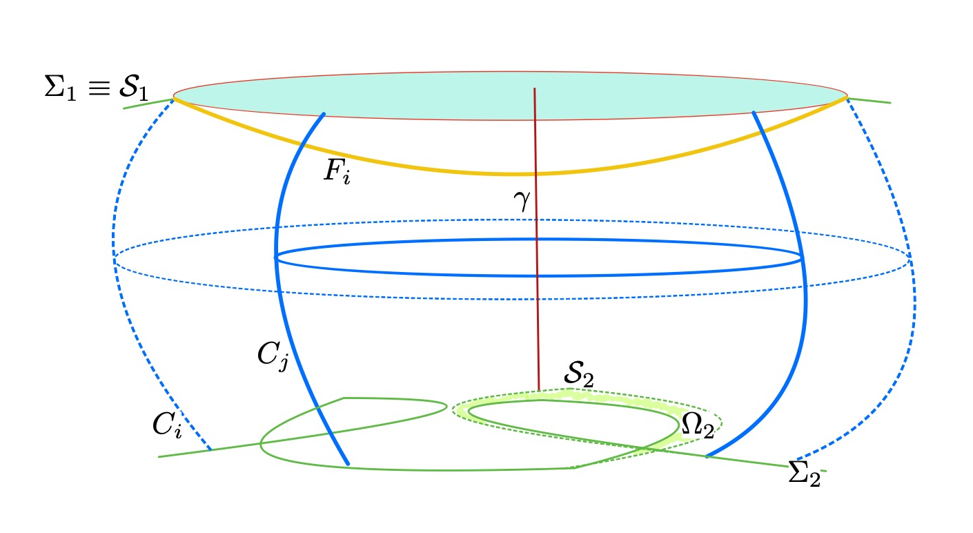
Figure 4: Quasi-embedded case

By Lemma 3.1, we obtain a two-sided properly embedded stable minimal hypersurface $\mathcal{F}\subset\mathcal{N}$ that is homologous to $\mathcal{S}_{1}$ and intersects $\gamma$. Observe that $\mathcal{F}\neq\mathcal{S}_{2}$ since $\mathcal{S}_{2}$ has strictly mean convex regions (cf. Figure 4). As in Case 1, in a finite number of steps (depending on ${\bf d}$ and $\epsilon>0$ of Theorem 4.1), we can show that there exists a properly embedded stable hypersurface $\mathcal{F}\subset\mathcal{N}$ such that $\mathcal{N}\setminus\mathcal{F}=\mathcal{N}_{1}\cup\mathcal{N}_{2}$, where $\mathcal{N}_{2}$ is a product manifold with boundaries $\mathcal{S}_{1}=\Sigma_{1}$ and $\mathcal{F}$; and $A$ is the region between $\mathcal{S}_{2}$ and $\mathcal{F}$ in $\mathcal{N}$ and such that ${\rm Tub}_{\epsilon}(\mathcal{F})\cap\mathcal{S}_{2}\neq\emptyset$. Therefore, as before, $\mathcal{N}_{1}$ is also a product manifold over $\mathcal{S}_{2}$ (or $\mathcal{F}$). Hence, $\overline{\mathcal{N}}$ is isometric to the product manifold $\Sigma_{1}\times[0,{\bf d}]$ and $\Sigma_{2}=\Sigma_{1}\times\left\{{\bf d}\right\}$; in particular $\Sigma_{2}$ must be stable, a contradiction. This proves Case 1. ∎

Case 2: $\Sigma_{1}$ and $\Sigma_{2}$ are not stable.

Proof of Case 2.

As in Case 2, we will construct strictly mean convex domains associated to the first eigenfunction of the Jacobi operator. Let $D_{k}\subset\Sigma_{k}$ be a geodesic ball large enough with smooth boundary centered at $x_{k}\in\Sigma_{k}$ so that the first eigenvalue of the Jacobi operator of satisfies $\lambda_{1}^{k}\leq-\tau$, for some $\tau>0$. Denote by $\phi_{k}:D_{k}\to\hbox{\bb R}^{+}$ the first eigenfunction associated to $\lambda_{1}^{k}$ and extend it by zero, that is, $\Phi_{k}(p)=\phi_{k}(p)>0$ for $p\in D_{k}$ and $\Phi_{k}(p)=0$ for $p\in\Sigma_{k}\setminus B_{k}$.

For $\tau^{\prime}>0$ small enough, define

$$\Sigma_{k}^{s}:=\left\{{\rm exp}_{p}(s\Phi_{k}(p)N_{k}(p))\,:\,\,p\in\Sigma_{k}\right\},$$

where $N_{k}$ is the unit normal along $\Sigma_{k}$ such that $N_{k}(x_{k})$ point towards $\mathcal{N}$, $k=1,2$. Shrinking $\tau^{\prime}>0$ if necessary, we can assume that the sets $\Omega_{k}:=\bigcup_{s\in[0,\tau^{\prime}]}\Sigma_{k}^{s}$, $k=1,2$, do not intersect. Also, by the First Variation Formula for the Mean Curvature (2.6) and shrinking $\tau^{\prime}>0$ again if necessary, $\Sigma_{k}^{s}$ is mean convex (and strictly mean convex in some regions) in the smooth regions with respect to the orientation pointing toward $\tilde{\mathcal{N}}:=\mathcal{N}\setminus(\Omega_{1}\cup\Omega_{2})$. Then, $\partial\tilde{\mathcal{N}}:=\mathcal{S}_{1}\cup\mathcal{S}_{2}\subset\Sigma_{1}\cup\partial\Omega_{2}$, where $\mathcal{S}_{1}\subset\partial\Omega_{1}$ and $\mathcal{S}_{2}\subset\Sigma_{2}\neq\emptyset$. $\tilde{\mathcal{N}}$ is piece-wise mean convex, the smooth pieces intersecting at angles less than $\pi$.

Fix $q_{1}\in\mathcal{S}_{1}$, ${\bf d}:={\rm dist}_{\mathcal{N}}(q_{1},\mathcal{S}_{2})$ and $\gamma:[0,{\bf d}]\to\mathcal{N}$ a minimizing geodesic such that $|\gamma|={\bf d}={\rm dist}_{\mathcal{N}}(q_{1},q_{2})$. We can assume that $q_{i}\in\mathcal{S}_{i}$ belong to the regular part, $i=1,2$. By Lemma 3.1, we obtain a two-sided properly embedded stable minimal hypersurface $\mathcal{F}\subset\mathcal{N}$ that is homologous to $\mathcal{S}_{1}$ and intersects $\gamma$. Observe that $\mathcal{F}\neq\mathcal{S}_{k}$ since $\mathcal{S}_{k}$ has strictly mean convex regions, $k=1,2$.

Thus, as in Case 1 and Case 2, we can construct a finite number (depending on ${\bf d}$ and $\epsilon>0$ of Theorem 4.1) $\mathcal{F}_{k}$, $k\in\left\{1,\ldots,m\right\}$, of pairwise disjoint, orientable, stable properly embedded minimal hypersurfaces, each one with an embedded, well-oriented and of bounded extrinsic geometry $\epsilon-$tube; $\epsilon>0$ is uniform, such that

• if $m>1$, then ${\rm Tub}_{\epsilon}(\mathcal{F}_{k})\cap{\rm Tub}_{\epsilon}(\mathcal{F}_{k-1})\neq\emptyset$ for all $k\in\left\{1,\ldots,m-1\right\}$;

• $\mathcal{S}_{1}\cap{\rm Tub}_{\epsilon}(\mathcal{F}_{1})\neq\emptyset$ and $\mathcal{S}_{2}\cap{\rm Tub}_{\epsilon}(\mathcal{F}_{m})\neq\emptyset$.

Thus, the second item above and Theorem ${\rm\tilde{A}}$ imply that $\mathcal{F}_{1}$ is parallel to $\mathcal{S}_{1}$; in particular $\Sigma_{1}$ must be stable, a contradiction. This proves Case 2. ∎

Hence, Case 1 and Case 2 prove Claim B. ∎

Finally, Claim A and Claim B prove Theorem 5.2. ∎

6 Parabolic area-minimizing hypersurfaces

Let $\mathcal{M}^{n}$, $3\leq n\leq 7$, be a complete orientable manifold of bounded geometry and $\Sigma^{n-1}\subset\mathcal{M}^{n}$ be a complete, orientable, non-compact hypersurface; $N$ a unit normal along $\Sigma$. Assume that $\overline{Ric}\geq 0$ and $\Sigma\subset\mathcal{M}$ is area-minimizing ${\rm mod}(2)$ and parabolic. Then, $\Sigma$ is properly embedded, has an embedded $\epsilon-$tubular neighborhood ${\rm Tub}_{\epsilon}(\Sigma)$ (cf. Theorem 3.2), is totally geodesic and $\overline{Ric}(N,N)\equiv 0$ along $\Sigma$ (cf. Proposition 2.1 and [56]).

Fix a point $p\in\Sigma$ and let $D_{p}(\epsilon)\subset\Sigma$ be the geodesic ball in $\Sigma$ centered at $p\in\Sigma$ of radius $\epsilon>0$. We might choose $\epsilon_{0}>0$ small enough so that $D_{p}(\epsilon)$ is topologically a ball and $\partial D_{p}(\epsilon)$ is smooth for all $0<\epsilon<\epsilon_{0}$. Let $\left\{K_{i}\right\}_{i\in\hbox{\bbp N}}$ be an exhaustion of $\Sigma$ by relatively compact sets so that $\overline{D_{p}(\epsilon_{0})}\subset K_{1}$, $K_{i}\subset K_{j}$, $i<j$, and $\partial K_{i}$ is smooth for all $i\in\hbox{\bb N}$.

Consider the embedding $F:\Sigma\times[-\epsilon,\epsilon]\to\mathcal{M}^{n}$ given by the exponential map $F(p,t)={\rm exp}_{p}(tN(p))$. Shrinking $\delta_{0}$ if necessary, we can assume that any normal geodesic starting at any point $q\in\overline{D_{p}(\epsilon_{0})}$ does not develop focal points (in any direction of the normal). For each $t\in[-\delta_{0},\delta_{0}]$ and $\epsilon\in(0,\epsilon_{0})$, denote by $\tilde{C}(\epsilon,t)$ the translation of $\partial D_{p}(\epsilon)$ by the exponential map at distance $t$; that is, $\tilde{C}(\epsilon,t)=F\left(\partial D_{p}(\epsilon),t\right)$.

Moreover, set $\mathcal{A}_{i}(\epsilon)=K_{i}\setminus\overline{D_{p}(\epsilon)}$ and consider the harmonic function $f_{i}^{\epsilon,t}:\mathcal{A}_{i}(\epsilon)\to\hbox{\bb R}$ given by

$$\left\{\begin{matrix}\Delta f_{i}^{\epsilon,t}=0&\text{ on }&\mathcal{A}_{i}(\epsilon),\\[2.84526pt] f_{i}^{\epsilon,t}=t&\text{ along }&\partial D_{p}(\epsilon),\\[2.84526pt] f_{i}^{\epsilon,t}=0&\text{ along }&\partial K_{i},\\ \end{matrix}\right.$$

and denote by $S_{i}^{\epsilon,t}$ the graph of $f_{i}^{\epsilon,t}$ under the exponential map; that is,

$$S_{i}^{\epsilon,t}=\left\{{\rm exp}_{q}(f_{i}^{\epsilon,t}(q)N(q))\,:\,\,q\in\mathcal{A}_{i}(\epsilon)\right\}.$$

Then, it is clear that $\partial S_{i}^{\epsilon,t}=\tilde{C}(\epsilon,t)\cup\partial K_{i}$. Denote by $\tilde{D}(\epsilon,t)$ the area-minimizing hypersurface with boundary $\tilde{C}(\epsilon,t)$. Now, we need to prove:

Lemma 6.1.

Fix $\epsilon\in(0,\epsilon_{0})$ and $t\in[-\delta_{0},\delta_{0}]$. Then, there exists $i_{0}\in\hbox{\bb N}$, depending on $\epsilon$, $t$ and the upper bound for the sectional curvature, so that

$$\mathcal{H}^{n-1}(S_{i}^{\epsilon,t})<\mathcal{H}^{n-1}(K_{i})+\mathcal{H}^{n-1}(\tilde{D}(\epsilon,t))\text{ for all }i\geq i_{0}.$$

Proof.

Consider the smooth map $F_{i}:\mathcal{A}_{i}(\epsilon)\to\mathcal{M}$ given by $F_{i}(q)={\rm exp}_{q}(f_{i}^{\epsilon,t}(q)N(q))$. Then,

$$\mathcal{H}^{n-1}(S_{i}^{\epsilon,t})=\int_{\mathcal{A}_{i}(\epsilon)}\left|{\rm Jac}F_{i}\right|d\Sigma,$$

where $d\Sigma$ is the volume element in $\Sigma$. Hence, we need to estimate the Jacobian $\left|{\rm Jac}F_{i}\right|$.

Let $q\in\mathcal{A}_{i}(\epsilon)$ and $\left\{e_{j}\right\}_{j=1,\ldots,n-1}\in T_{q}\mathcal{A}_{i}(\epsilon)$ be an orthonormal basis so that

$$e_{1}=\frac{\nabla f_{i}^{\epsilon,t}}{|\nabla f_{i}^{\epsilon,t}|}\text{ and }g\left(e_{j},\nabla f_{i}^{\epsilon,t}\right)=0\text{ for }j=2,\ldots,n-1;$$

we can do this choice for all $q\in\mathcal{A}_{i}(\epsilon)\setminus\mathcal{C}$, where $\mathcal{H}^{n-1}(\mathcal{C})=0$. Consider the geodesic $\alpha_{i}:(-\tau,\tau)\to\mathcal{A}_{i}(\epsilon)$ with initial conditions $\alpha_{j}(0)=q$ and $\alpha_{j}^{\prime}(0)=e_{j}$. Consider the variation by normal geodesics $g_{j}(s,r):={\rm exp}_{\alpha_{j}(s)}(rf_{i}^{\epsilon,t}(\alpha_{j}(s))N(\alpha_{j}(s)))$ and set

$$\tilde{J}_{j}(r):=\left.\frac{d}{ds}\right|_{s=0}g_{j}(s,r)$$

with initial condition $\tilde{J}_{j}(0)=e_{j}$. Consider also the Jacobi field associated to the variation $g^{0}_{j}(s,r):={\rm exp}_{\alpha_{j}(s)}(rN(\alpha_{j}(s)))$, that is,

$$J_{j}(r):=\left.\frac{d}{ds}\right|_{s=0}g^{0}_{j}(s,r)$$

with, also, initial condition $J_{j}(0)=e_{j}$. Observe that, since $\Sigma$ is totally geodesic and $\left\{e_{j}\right\}_{j=1,\ldots,n-1}$ is orthonormal then

$$\left\{\gamma_{q}^{\prime}(r),J_{1}(r),\ldots,J_{n-1}(r)\right\}$$

is orthogonal at $q_{r}:=\gamma_{q}(r)={\rm exp}_{q}(rN(q))$ for all $r>0$; in particular, it is a basis along $\gamma_{q}$. This follows from the fact that the tangential part (along the geodesic) of $J_{j}$ is a linear field (cf. [27, page 179]).

Set $\bar{r}:=(f_{i}^{\epsilon,t})(q)$ and $\bar{q}:=\gamma_{q}(\bar{r})\in S_{i}^{\epsilon,t}$. Then, $\left\{\tilde{J}_{j}(1)\right\}_{j=1}^{n-1}$ is a basis at $T_{\bar{q}}S_{i}^{\epsilon,t}$ and it can be orthogonally decomposed as

$$\tilde{J}_{j}(1)=J_{j}(\bar{r})+e_{j}(f_{i}^{\epsilon,t})\gamma_{q}^{\prime}(\bar{r})$$

and hence

$$\tilde{J}_{1}(1)\wedge\ldots\wedge\tilde{J}_{n-1}(1)=J_{1}(\bar{r})\wedge\ldots\wedge J_{n-1}(\bar{r})+e_{1}(f_{i}^{\epsilon,t})\gamma_{q}^{\prime}(\bar{r})\wedge J_{2}(\bar{r})\wedge\ldots\wedge J_{n-1}(\bar{r}),$$

and now, since $J_{1}(\bar{r})\wedge J_{2}(\bar{r})\wedge\ldots\wedge J_{n-1}(\bar{r})$ and $\gamma_{q}^{\prime}(\bar{r})\wedge J_{2}(\bar{r})\wedge\ldots\wedge J_{n-1}(\bar{r})$ are orthogonal, we obtain

$$\left|\tilde{J}_{1}(1)\wedge\ldots\wedge\tilde{J}_{n-1}(1)\right|^{2}=\left|J_{1}(\bar{r})\wedge\ldots\wedge J_{n-1}(\bar{r})\right|^{2}+\frac{\left|\nabla f_{i}^{\epsilon,t}\right|^{2}}{\left|J_{1}(\bar{r})\right|^{2}}\left|J_{1}(\bar{r})\wedge\ldots\wedge J_{n-1}(\bar{r})\right|^{2}.$$

Using now that $\overline{Ric}\geq 0$, it is well-known (see [24]) that

$$\left|J_{1}(\bar{r})\wedge\ldots\wedge J_{n-1}(\bar{r})\right|\leq\left|e_{1}\wedge\ldots\wedge e_{n-1}\right|=1$$

and hence

$$\mathcal{H}^{n-1}(S_{i}^{\epsilon,t})=\int_{\mathcal{A}_{i}(\epsilon)}\left|\tilde{J}_{1}(1)\wedge\ldots\wedge\tilde{J}_{n-1}(1)\right|\,d\Sigma\leq\int_{\mathcal{A}_{i}(\epsilon)}\sqrt{1+\frac{\left|\nabla f_{i}^{\epsilon,t}\right|^{2}}{\left|J_{1}(\bar{r})\right|^{2}}}d\Sigma.$$ (6.1)

Finally, we need to estimate the right-hand side of (6.1). First, since $|J_{1}(0)|=1$, then $\left|J_{1}\right|\geq\lambda>0$, for some $\lambda$ depending only on the upper bound of the sectional curvature. Second, using the inequality $\sqrt{1+x}\leq 1+x$ for all $x\geq 0$ applied to (6.1), we obtain

$$\begin{split}\mathcal{H}^{n-1}(S_{i}^{\epsilon,t})&\leq\mathcal{H}^{n-1}(\mathcal{A}_{i}(\epsilon))+\frac{1}{\lambda^{2}}\int_{\mathcal{A}_{i}(\epsilon)}\left|\nabla f_{i}^{\epsilon,t}\right|^{2}\,d\Sigma\\ &=\mathcal{H}^{n-1}(K_{i})+\frac{1}{\lambda^{2}}\int_{\mathcal{A}_{i}(\epsilon)}\left|\nabla f_{i}^{\epsilon,t}\right|^{2}\,d\Sigma-\mathcal{H}^{n-1}(D_{p}(\epsilon)).\end{split}$$

Thus, since $\Sigma$ is parabolic (see [30, Theorem 10.1]), there exists $i_{0}\in\hbox{\bb N}$ so that

$$\int_{\mathcal{A}_{i}(\epsilon)}\left|\nabla f_{i}^{\epsilon,t}\right|^{2}\,d\Sigma<\lambda^{2}\mathcal{H}^{n-1}(D_{p}(\epsilon))\text{ for all }i\geq i_{0}$$

and the proof is completed. ∎

The above lemma implies that if $\Sigma\subset\mathcal{M}$ is properly embedded, parabolic, orientable, area-minimzing ${\rm mod}(2)$ hypersurface; then it satisfies the Maximum Principle at Infinity. Actually, it proves more, a local splitting theorem as in [3].

Remark 6.1 (Douglas Criterion for the Plateau Problem).

When we want find area-minimizing hypersurfaces (currents) in $\mathcal{M}$ with two (disjoint) boundary components $\Gamma_{1}\cup\Gamma_{2}$ that is connected; we must ensure that there exists a comparison hypersurface $S\subset\mathcal{M}$, $\partial S=\Gamma_{1}\cup\Gamma_{2}$, of area less than $\mathcal{H}^{n-1}(\Sigma_{1})+\mathcal{H}^{n-1}(\Sigma_{2})$, where $\Sigma_{i}$ are least-area hypersurfaces bounding $\Gamma_{i}$, $i=1,2$. In such case, any area-minimizing hypersurface $\mathcal{A}\subset\mathcal{M}$ with $\partial\mathcal{A}=\Gamma_{1}\cup\Gamma_{2}$ must be connected.

Theorem 6.1.

Let $\mathcal{M}^{n}$, $3\leq n\leq 7$, be a complete orientable manifold of bounded geometry and $\overline{Ric}\geq 0$. Let $\Sigma\subset\mathcal{M}$ be complete, parabolic, oriented, area-minimizing ${\rm mod}(2)$ hypersurface. Then, the universal covering $\widetilde{\mathcal{M}}$ of $\mathcal{M}$ is isometric to $\Sigma\times\hbox{\bb R}$ with the product metric.

Proof.

As explained in the beginning of this section, $\Sigma$ is properly embedded and has an embedded $\epsilon-$tubular neighborhood. Consider the hypersurfaces $S_{i}^{\epsilon,t}$ constructed above. From Lemma 6.1 and using the Douglas Criterion for the Plateau Problem, for each $i\geq i_{0}$, there exists a compact connected area-minimizing hypersurface $\tilde{S}^{\epsilon,t}_{i}$, smooth up to $n\leq 7$ (see [54, 56]), so that $\partial\tilde{S}^{\epsilon,t}_{i}=\tilde{C}(\epsilon,t)\cup\partial K_{i}$. Moreover, by the Maximum Principle $\tilde{S}^{\epsilon,t}_{i}\subset\Sigma\times(0,t)$.

Since $\tilde{S}^{\epsilon,t}_{i}$ is area-minimizing we have area and curvature estimates on compact sets as we did in Section 3. Hence, we can follow the arguments in Section 3 to obtain a subsequence of $\left\{\tilde{S}^{\epsilon,t}_{i}\right\}_{i\in\hbox{\bbp N}}$ that converges to a connected area-minimizing hypersurface $\tilde{S}^{\epsilon,t}_{\infty}$ such that $\partial\tilde{S}^{\epsilon,t}_{\infty}=\tilde{C}(\epsilon,t)$. Next, letting $\epsilon\to 0$ and keeping $t\in(0,\delta_{0}]$ fixed, one obtains an area-minimizing hypersurface $\tilde{S}^{t}_{\infty}$ in $\mathcal{M}\setminus\left\{\gamma_{q}(t)\right\}$ such that:

• it is embedded;

• may a priori have infinite topological type;

• proper by construction;

• smooth outside $\gamma_{q}(t)$ and across $\gamma_{q}(t)$ up to $n\leq 7$ (see [56, Section 3.4]).

Then, following [3, page 464], we can show that the family $\left\{S^{t}_{\infty}\right\}_{t\in[-\delta,\delta]}$, for some $\delta\leq\delta_{0}$ if necessary, forms a $C^{0}$ foliation of a region of $\mathcal{M}$, where $S_{\infty}^{0}=\Sigma$ is a leaf of this foliation. In particular, all the $S_{\infty}^{t}$ are quasi-isometric to $\Sigma$ by Schoen-Simon-Yau Curvature Estimate, shrinking $\delta>0$ if necessary. Therefore, since all the $S_{\infty}^{t}$ are also stable, $\left\{S^{t}_{\infty}\right\}_{t\in[-\delta,\delta]}$ is a foliation by proper, totally geodesic hypersurfaces of a region of $\mathcal{U}\subset\mathcal{M}$. Hence, Lemma 7.1 implies that $\mathcal{U}$ is isometric to the Riemannian product $\Sigma\times[-\delta,\delta]$.

As in [3, page 465], we can also show that each leaf of the foliation is area-miminizing (and parabolic); thus we can iterate this process indefinitely to finally prove the result. ∎

7 Concluding remarks

The following lemma is well known in this subject and we welcome a reader to tell us to whom it should be atributed.

Lemma 7.1.

Let $\Sigma^{n-1}$ be a complete embedded orientable minimal hypersurface in a complete orientable manifold $\mathcal{M}^{n}$ of non-negative Ricci curvature. Suppose that for some $\delta>0$ the map $F:\Sigma\times[0,\delta]\to\mathcal{M}$, $F(p,t):={\rm exp}_{p}(tN(p))$, where $N$ is a unitary normal to $\Sigma=F(\Sigma\times\left\{0\right\})$, is an embedding.

If there is a $\bar{t}\in(0,\delta]$ such that the equidistant $\Sigma(\bar{t})=F(\Sigma\times\left\{\bar{t}\right\})$ is a minimal hypersurface, then $F:\Sigma\times[0,\bar{t}]\to\mathcal{M}$ is an isometry onto its image, where $\Sigma\times[0,\bar{t}]$ has the product metric $\sigma+dt^{2}$; $\sigma$ the induced metric on $\Sigma$.

Proof.

The geodesics $\gamma_{p}(t)=F(p,t)$, $t\in[0,\delta]$, are minimizing, $F$ has no critical points so there are no conjugate points on $\gamma_{p}$ and no two geodesics $\gamma_{p}$, $\gamma_{q}$ intersect if $p\neq q$.

Let $d={\rm dist}_{\mathcal{M}}\left(F(p,t),F(\Sigma\times\left\{0\right\})\right)=t$ denote the distance function on $F(\Sigma\times[0,\delta])\subset\mathcal{M}$ to $\Sigma=F(\Sigma\times\left\{0\right\})$; so $\overline{\nabla}d=N_{t}$ on $F(\Sigma\times[0,\delta])$ where $N_{t}$ is the unitary normal along the equidistant $\Sigma(t)=F(\Sigma\times\left\{t\right\})$, $t\in[0,\delta]$, such that $N_{0}=N$.

The First Variation Formula for the Mean Curvature (2.6) of the equidistant hypersurfaces $\Sigma(t)$, $t\in[0,\delta]$, is:

$$H^{\prime}(p,t)=|A_{t}(p)|^{2}+\overline{Ric}(\overline{\nabla}d_{F(p,t)},\overline{\nabla}d_{F(p,t)})\geq 0,$$

where $A_{t}(p)$ is the second fundamental of $\Sigma(t)$ at $\gamma_{p}(t)$; and the sign of $(n-1)H(p,t)={\rm Trace}\left(A_{t}(p)\right)$ is such that

$$A_{t}(p)(u)=-\overline{\nabla}_{u}\left(\overline{\nabla}d_{F(p,t)}\right),\,\,u\in T_{F(p,t)}\Sigma(t).$$

Thus, $H(p,0)=H(p,\bar{t})=0$ for all $p\in\Sigma$ and, since $H$ is non-decreasing on $t$, $H(p,t)=0$ for all $(p,t)\in\Sigma\times[0,\bar{t}]$. Each equidistant $\Sigma(t)$, $t\in[0,\bar{t}]$, is totally geodesic, $A_{t}\equiv 0$ for all $t\in[0,\bar{t}]$, and $\overline{Ric}(\overline{\nabla}d,\overline{\nabla}d)\equiv 0$ as well in this region $\mathcal{N}:=F(\Sigma\times[0,\bar{t}])$.

Observe that $\overline{\nabla}d$ is parallel in $\mathcal{N}$; $\overline{\nabla}_{v}\overline{\nabla}d=0$ for all $v\in T_{F(p,t)}\mathcal{M}$. To see this decompose a tangent vector $v\in T_{F(p,t)}\mathcal{N}$ into its part tangent to the equidistant $\Sigma(t)$ and normal to $\Sigma(t)$; i.e., parallel to $\overline{\nabla}d$. Since $A_{t}\equiv 0$, $\overline{\nabla}_{v}\overline{\nabla}d=0$ for all $v$ tangent to $\Sigma(t)$ and $\overline{\nabla}_{\overline{\nabla}d}\overline{\nabla}d=0$, so $\overline{\nabla}_{v}\overline{\nabla}d=0$ for all $v\in T_{F(p,t)}\mathcal{N}$.

Next, notice that $\overline{\nabla}d$ is a Killing field in $\mathcal{N}$:

$$\langle\overline{\nabla}_{X}\overline{\nabla}d,Y\rangle+\langle\overline{\nabla}_{Y}\overline{\nabla}d,X\rangle=0\text{ for any }X,Y\in T_{F(p,t)}\mathcal{N}.$$

To check the above equation again decompose $X$ and $Y$ into their tangent and normal parts. Hence the map $\Sigma(t)\to\Sigma(s)$ given by the integral curves $\gamma_{p}(t)$ of $\overline{\nabla}d$ is an isometry for $t,s\in[0,\bar{t}]$. Thus $F$ preserves the scalar product of the metric $\sigma+dt^{2}$, which proves the lemma. ∎

Finally, the results that contain this paper can be used to obtain topological obstructions to the existence of manifolds with non-negative Ricci curvature (see [53] and references therein).

Appendix

Theorem 7.1.

Let $(\hbox{\bb S}^{2},g)$ be endowed with a metric of positive curvature, then a complete embedded geodesic on $(\hbox{\bb S}^{2},g)$ is compact.

Proof.

Let $\gamma:\hbox{\bb R}\to(\hbox{\bb S}^{2},g)$ be a complete (parametrized by arc-length) embedded geodesic. If $\gamma$ is not compact then $\overline{\gamma}=\mathcal{L}$ is a geodesic lamination with a limit leaf $C$ (a geodesic embedded and complete) and there is a point $q\in C$ that is a limit of points $p_{n}\in\gamma$ that diverge on $\gamma$.

Let $\vec{n}$ be a unit vector field to $C$. The curvature of $(\hbox{\bb S}^{2},g)$ is bounded so there exists $\epsilon>0$ and $\delta>0$ such that for all $x=C(t_{0})$, then the map $\psi:[t_{0}-\delta,t_{0}+\delta]\times[-\epsilon,\epsilon]\to(\hbox{\bb S}^{2},g)$ given by

$$\psi(t,s):={\rm exp}_{C(t)}(s\vec{n}(C(t)))$$

is a diffeomorphism. $\psi$ extends to an immersion $\Psi:\hbox{\bb R}\times[-\epsilon,\epsilon]\to(\hbox{\bb S}^{2},g)$.

For each $s\in[-\epsilon,\epsilon]$, $C_{s}:\hbox{\bb R}\to(\hbox{\bb S}^{2},g)$, given by $C_{s}(t):=\Psi(t,s)$, is the equidistant (of distance $s$) from $C$. Its geodesic curvature vector points away from $C$.

Think locally of $C$ as horizontal and the $C_{s}$ as well, the vertical segments are the geodesics $\beta_{t}:[-\epsilon,\epsilon]\to(\hbox{\bb S}^{2},g)$, given by $\beta_{t}(s)=\Psi(t,s)$. Pull back the metric of $(\hbox{\bb S}^{2},g)$ to $\hbox{\bb R}\times[-\epsilon,\epsilon]$ by $\Psi$; call it $\tilde{g}$ (cf. Figure 5).

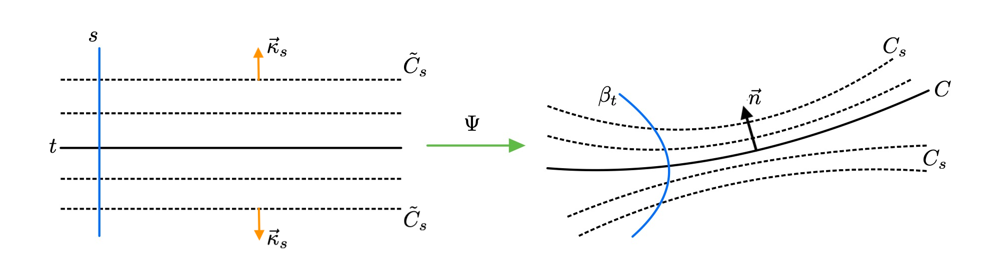
Figure 5: The immersion $\Psi$

Since $\gamma$ is embedded, the tangent lines to $\gamma$ at $p_{n}$ converge to the tangent line to $C$ at $q$ as $n\to\infty$. The neighborhood $W(q):=\left\{\beta_{t}(s)\,:\,\,t\in[\bar{t}-\delta,\bar{t}+\delta],\,s\in[0,\epsilon]\right\}$ lifts isometrically to $[\bar{t}-\delta,\bar{t}+\delta]\times[0,\epsilon]$ by $\Psi^{-1}$. Without lost of generality, we can assume $p_{n}\in W(q)$ and $p_{n}=\beta_{t_{n}}(s_{n})$ for some $t_{n}\in[\bar{t}-\delta,\bar{t}+\delta]$ and $s_{n}\in(0,\epsilon)$ such that $t_{n}\to\bar{t}$ and $s_{n}\to 0$ as $n\to\infty$.

Fix $n$ big enough and, for notational convenience, reparametrise $C$ such that $t_{n}=0$ and $s_{n}=s(0)\in(0,\epsilon)$. Let $\tilde{\gamma}$ be the component of $\Psi^{-1}(\gamma)$ containing $\Psi^{-1}(p_{n})=(0,s(0))$. $\tilde{\gamma}$ is a geodesic that intersects the vertical geodesic $\tilde{\beta}_{0}:=\left\{0\right\}\times[0,\epsilon]$ at the point $(0,s(0))$. Observe that $\tilde{\gamma}$ can not be locally above the equidistant $\tilde{C}_{s(0)}$ at $(0,s(0))$ since the geodesic curvature of the equidistant $\tilde{C}_{s(0)}$ is positive, the curvature vector is pointing up.

So, we can always choose one of the components of $\tilde{\gamma}\setminus\left\{(0,s(0))\right\}$ so that the tangent vector to the component at $(0,s(0))$ is going down. Orient this component, $\tilde{\gamma}^{+}(t)$, in the direction it is going down at $(0,s(0))$. Without lost of generality, we can assume $\tilde{\gamma}^{+}(t)$ goes down for $t\in(0,\omega)$, $\omega>0$ small.

Then, $\tilde{\gamma}^{+}(t)$ is a geodesic arc making an (exterior) angle $\theta\in[\pi/2,\pi)$ with the vertical geodesic $\tilde{\beta}_{0}:=\left\{0\right\}\times[0,\epsilon]$, it can not be equal $\pi$ since $\gamma$ is embedded. Using that the geodesic curvature of the equidistants $\tilde{C}_{s}$ is positive, the curvature vector is pointing up, it is easy to observe that, if we write $\tilde{\gamma}^{+}(t)=(t,s(t))$, $s(t)$ is monotonically decreasing in $[0,\delta]$. In fact, the above argument remains true for all $0<t$ and hence, we consider the half-geodesic $\tilde{\gamma}^{+}:[0,+\infty)\to\hbox{\bb R}\times[0,\epsilon]$.

$\tilde{\gamma}^{+}$ strictly descends for all time (since it can not become tangent from above to an equidistant), so it is defined for all time and is asymptotic to some $\hbox{\bb R}\times\left\{\bar{s}\right\}$, $\bar{s}\in[0,\epsilon)$, as $t$ diverges. Thus the exterior angle $\alpha(t)$, that $\tilde{\gamma}$ makes with the vertical can be made as close to $\pi/2$ as desired, for $t$ large.

Fix $L\geq\delta$ and let $D(L)$ be the disk bounded by $\left(\left\{0\right\}\times[0,s(0)]\right)\cup\tilde{\gamma}^{+}\left([0,L]\right)\cup\left(\left\{L\right\}\times[0,s(L)]\right)\cup\left([0,L]\times\left\{0\right\}\right)$, then by the Gauss-Bonnet Theorem, we get

$$\int_{D(L)}\tilde{K}+\theta+\alpha(L)=\pi,$$

where $\theta$ and $\alpha(L)$ are the exterior angles at $(0,s(0))$ and $(L,s(L))$, respectively, and $\tilde{K}$ the Gauss curvature in $\left(\hbox{\bb R}\times[-\epsilon,\epsilon],\tilde{g}\right)$ (cf. Figure 6). Therefore, using that $\tilde{K}\geq A>0$, we obtain

$$0<\int_{D(\delta)}\tilde{K}\leq\pi-\theta-\alpha(L)\leq\pi/2-\alpha(L)\to 0,$$

as $L\to+\infty$; which is a contradiction.

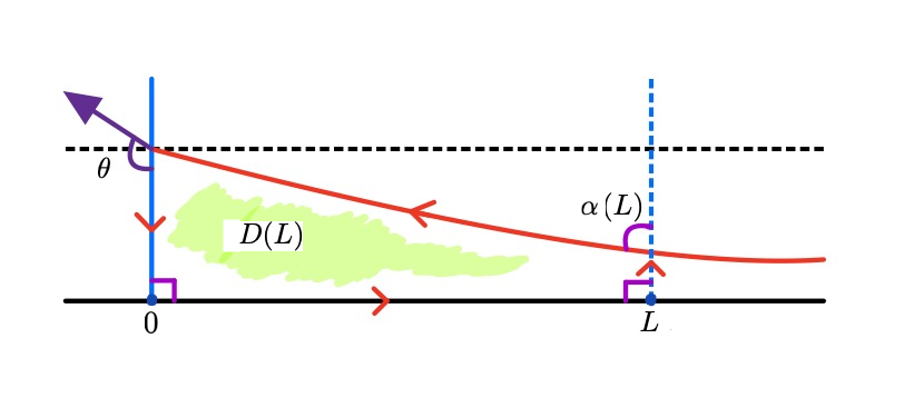
Figure 6: Disk bounded by $\left(\left\{0\right\}\times[0,s(0)]\right)\cup\tilde{\gamma}^{+}\left([0,L]\right)\cup\left(\left\{L\right\}\times[0,s(L)]\right)\cup\left([0,L]\times\left\{0\right\}\right)$

Remark 7.1.

We can extend this theorem to complete, non-compact, orientable surfaces $\mathcal{M}$ of positive curvature $\overline{K}>0$. Suppose $\gamma$ is a complete, non-compact, embedded geodesic of $\mathcal{M}$. It is not hard to show that there exists an $\epsilon>0$ such that $\epsilon-$tubular neighborhood ${\rm Tub}_{\epsilon}(\gamma)$ is embedded in $\mathcal{M}$. Our proof of Theorem 7.1 shows that if a geodesic $\tilde{\gamma}$ of $\mathcal{M}$ intersects ${\rm Tub}_{\epsilon}(\gamma)$, then $\tilde{\gamma}$ intersects $\gamma$.

In [29] the authors claim Theorem 7.1 extends to dimensions $n>2$: When $\mathcal{M}^{n}$ is closed, $\overline{K}>0$, a complete embedded geodesic $\gamma\subset\mathcal{M}$ must intersect every closed totally geodesic hypersurface of $\mathcal{M}$. However, the proof is not complete. We do not know if this holds for $n=3$.

∎

References

- [1]
- [2] L. Ambrosio, C. Mantegazza, Curvature and distance function from a manifold, J. Geom. Anal., 8 (1998) no. 5, 723–748. Dedicated to the memory of Fred Almgren.
- [3] M. Anderson, L. Rodríguez, Minimal surfaces and manifolds of non-negative Ricci curvature, Math. Ann., 284 (1989), 461–475.
- [4] L. Ambrosio, H. M. Soner, A level set approach to the evolution of surfaces of any codimension, J. Diff. Geom., 43 (1996), 693–737.
- [5] M. Anderson, curvature and volume renormalization of AHE metrics on manifolds, Math. Res. Lett., 8 (2001), no. 1-2, 171–188.
- [6] M. do Carmo, C.K. Peng, Stable complete minimal surfaces in are planes, Bull. Amer. Math. Soc. (N.S.) 1 (1979) no. 6, 903–906.
- [7] G. Catino, P. Mastrolia, A. Roncoroni, Two rigidity results for stable minimal hypersurfaces. arXiv:2209.10500.
- [8] J. Cheeger, D. Gromoll, On the Structure of Complete Manifolds of Nonnegative Curvature, Annals of Math., 96 (1972) no. 3, 413–443.
- [9] Q. Chen, Curvature estimates for stable minimal hypersurfaces in and , Annals of Global Anal. and Geom., 19 (2001), 177–184.
- [10] O. Chodosh, Brian White, Topics in GMT (math 258). https://web.stanford.edu/ ochodosh/GMTnotes.pdf.
- [11] O. Chodosh, M. Eichmair, V. Moraru, Splitting theorems for scalar curvature, Comm. Pure. Appl. Math., 72 (2019) no. 6, 1231–1242.
- [12] O. Chodosh, C. Li Stable minimal hypersurfaces in . arXiv:2108.11462v2.
- [13] O. Chodosh, C. Li, D. Stryker, Complete stable minimal hypersurfaces in positively curved 4-manifolds. arXiv:2202.07708.
- [14] J. Choe, A. Fraiser, Mean curvature in manifolds with Ricci curvature bounded from below, Comment. Math. Helv., 93 (2018), 55–69.
- [15] C. Croke, B. Kleiner, A warped product splitting theorem, Duke Math. J., 67 (1992) no. 3, 571–574.
- [16] C. De Lellis, J. Hirsch, A. Marchese, S. Stuvard, Regularity of area minimizing currents mod , Geom. Funct. Anal., 30 (2020), 1224–1336.
- [17] Q. Ding, Area-minimizing hypersurfaces in manifolds of Ricci curvature bounded below. arXiv:2017.11074v1.
- [18] Q. Ding, J. Jost, Y.L. Xin, Existence and non-existence of area minimizing hypersurfaces in manifolds of non-negative Ricci curvature, Amer. J. Math., 138 (2016) no. 2, 287–327.
- [19] R. Escobales, Riemannian submersions with totally geodesic fibers, J. Diff. Geom., 10 (1975), 253–276.
- [20] D. Fischer-Colbrie, R. Schoen, The structure of complete stable minimal surfaces in manifolds of nonnegative scalar curvature, Comm. Pure Appl. Math., 33 (1980) no. 2, 199–211.
- [21] T. Frankel, On the fundamental group of a compact minimal submanifold, Ann. ofMath., 83 (1966), 68–73.
- [22] G. Galloway, L. Rodríguez, Intersection of minimal surfaces, Geom. Ded., 39 (1991), 29–42.
- [23] J. Hadamard, Sur certaines propriètès des trajectoires en dynamique, J. Math. Pures Appl., 5 (1897) no. 3, 331–387.
- [24] E. Heintze, H. Karcher, A general comparison theorem with applications to volume estimates for submanifolds, Ann. Sci. l’E.N.S., 11 (1978) no. 4, 451–470.
- [25] D. Hoffman, W.H. Meeks III, The strong halfspace theorem for minimal surfaces, Invent. Math., 101 (1990), 373–377.
- [26] L. Jorge, F. Xavier, An inequality between exterior diameter and the mean curvature of bounded immersions, Math. Z., 112 (1981), 203–206.
- [27] H. Karcher, Riemannian comparison constructions, Volumen 5, Rheinische Friedrich-Wilhelms-Universität Bonn, Sonderforschungsbereich 256, Nichtlineare Partielle Differentialgleichungen (1987).
- [28] R. Langevin, H. Rosenberg, A Maximum Principle at Infinity for minimal surfaces and applications, Duke Math. J., 57 (1988) no. 3, 819–828.
- [29] R. Langevin, H. Rosenberg, Quand deux sous-variétés sont forcées par leur géométrie à se encontrer, Bulletin S.M.F., 120 (1992) no. 2, 227–235.
- [30] P. Li, Lectures on harmonic functions, (2004). http://citeseerx.ist.psu.edu/viewdoc/download?doi=10.1.1.77.1052.
- [31] P. Li, J. Wang, Stable minimal hypersurfaces in a nonnegatively curved manifold, J. Reine Ang. Math. (Crelles Journal), 566 (2004), 215–230.
- [32] G. Liu, 3-manifolds with non-negative Ricci curvature, Invent. Math., 193 (2013), 367–375.
- [33] L. Mazet, A general halfspace theorem for constant mean curvature surfaces, Amer. J. Math., 135 (2013) no. 3, 801–834.
- [34] L. Mazet, H Rosenberg, Minimal hypersurfaces of least area, J. Diff. Geom, 106 (2017) no. 2, 283–316.
- [35] F. Morgan, Geometric measure theory: A beginner’s guide, 5th ed., Academic Press, Inc., San Diego, CA, 2016.
- [36] W. Meeks, H. Rosenberg, The global theory of doubly periodic minimal surfaces, Invent. Math., 97 (1989), 351–379.
- [37] WH. Meeks, H. Rosenberg, The uniqueness of the helicoid, Annals of Math., 161 (2005), 727–758.
- [38] W. Meeks, H. Rosenberg The theory of minimal surfaces in , Comm. Math. Helvetici, 80 (2005), 811–858.
- [39] WH. Meeks, H. Rosenberg, Maximum Principles at infinity, J. Diff. Geom., 79 (2008) no. 1, 141–165.
- [40] V. Moraru, On area comparison and rigidity involving the scalar curvature, J. Geom. Anal., 26 (2014), 294–312.
- [41] O. Munteneau, J. Wang, Comparison Theorems for 3D manifolds with scalar curvature bound, II. Arxiv.
- [42] A. Pogorelov, On the stability of minimal surfaces, Soviet Math. Dokl., 24 (1981), 274–276.
- [43] A. Ros and H. Rosenberg, Properly embedded surfaces with constant mean curvature, Amer. J. Math., 132 (2010), 1429–1443.
- [44] H. Rosenberg, Hypersurfaces of constant curvature in space forms, Bull. Sc. Math. série, 117 (1993), 211–239.
- [45] H. Rosenberg, Intersection of minimal surfaces of bounded curvature, Bull. Sci. Math., 125 (2001) no. 2, 161–168.
- [46] H. Rosenberg, Minimal surfaces in , Illinois J. Math., 46 (2002) no. 4, 1177–1195.
- [47] H. Rosenberg, F. Schulze, J. Spruck, The Half-space property and entire positive minimal graphs in , J. Diff. Geom., 95 (2013), 321–336.
- [48] H. Rosenberg, R. Souam, E. Toubiana, General curvature estimates for stable surfaces in manifolds and applications, J. Diff. Geom., 84 (2010), 623–648.
- [49] R. Schoen, Estimates for stable minimal surfaces in three-dimensional manifolds, Seminar on minimal submanifolds, Ann. of Math. Stud., 103, Princeton Univ. Press (1983), 111-126.
- [50] R. Schoen, L. Simon, Regularity of stable minimal hypersurfaces, Comm. Pure and Appl. Math., 34 (1981), 742–797.
- [51] R. Schoen and S.T. Yau, Harmonic maps and the topology of stable hypersurfaces and manifolds of nonnegative Ricci curvature, Comm. Math. Helv. 39 (1976), 333–341.
- [52] R. Schoen, L. Simon, S.-T. Yau, Curvature estimates for minimal hypersurfaces. Acta Math., 134 (1975), 275–288.
- [53] Z. Shen, C. Sormani, On the topology of open manifolds with non-negative Ricci curvature, Comm. Math. Anal., Conference 1 (2008), 20–34. ISSN: 1938-9787.
- [54] L. Simon, Lectures on Geometric Measure Theory. Proc. Centre Math. Anal., Austral. Nat. Univ., Canberra 3 (1983).
- [55] A. Song, Embeddedness of least area minimal hypersurfaces, J. Diff. Geom., 110 (2018), 345–377.
- [56] N. Wickramasekera, Regularity of stable minimal hypersurfaces: Recent advances in the theory and applications, Surveys in differential geometry, 19 (2014), 231–301.