Qualitative analysis of strictly non-Volterra quadratic dynamical systems with continuous time
Abstract
In this article, a continuous analogue of strictly non-Volterra quadratic dynamical systems with continuous time and points of equilibrium is investigated, a phase portrait of the system is constructed, numerical solutions are found, and a comparative analysis is carried out with a particular solution of the system.
keywords:
quadratic stochastic operators, phase portrait, equilibrium positions, trajectory, qualitative analysis.34C05, 34C40, 34C60, 37C25 \VOLUME30 \NUMBER1 \DOIhttps://doi.org/10.46298/cm.10528 {paper}
1 Introduction
The main theoretical and practical studies on the study of the dynamics of a free population, various problems of physics and economics are reduced to dynamic systems. In this, a special role is played by the quadratic stochastic operators. In this regard, quadratic operators attract the attention of specialists in various fields of mathematics and its applications (see for example [Bern2], [Ulam21]). Therefore, studies of quadratical stochastic operators remain relevant. The concept of a quadratic stochastic operator was first formulated in the article [Bern2]. S. Ulam [Ulam21] posed the problem of studying the behavior of the trajectories of quadratic stochastic operators. This problem is mainly solved for Volterra operators (see [Gani5], [Gani6], [Gani7], [Gani8], [Mukh14], [Gani4]) of discrete time. In [Tian19], a definition of strictly non-Volterra quadratic stochastic operators is introduced, which is a subclass of non-Volterra operators. But the class of non-Volterra operators has been little studied. Depending on the problem, either continuous time can be considered (when the states of the system are of interest at each moment), or discrete (when the states of the system are of interest at separate isolated moments of time). System behavior depends on parameters, the exact values of which are often unknown. It is fundamentally impossible to solve such problems numerically for all possible parameter values. Therefore, methods are needed that will make it possible to analyze the behavior of solutions to a dynamical system without using a computer. As we noted above, quadratic stochastic operators of the Volterra class in discrete time have been studied quite deeply. Here are some of them [Rozi17], [Gani9], [Kest12], [Lyub13], [Rozi18]. Also, quadratic stochastic operators with continuous time, that is, various modifications of the predator and prey model and other models, have been studied by many authors in [Ange1], [Tian19] and [Huan10]. In turn, the class of strictly non-Volterra quadratic stochastic operators with continuous time (hereinafter referred to as quadratic dynamical systems) has been studied relatively less. Since there is no general theory studying such operators. Note the works [Rasu16]. The most useful aspect of the qualitative theory of dynamical systems, be more correct, dynamical systems with continuous time, is that many important properties of solutions can be predicted in advance without having explicit solutions of the equations. In this article, we study a qualitative analysis of a quadratic dynamical system, a continuous analogue of the non quadratic stochastic Volterra operator from [Mukh15]. The system is shown to come to a simple differential equation, solutions are found, and they are studied separately. Equilibrium points of the system are found and a phase portrait is given. Analytical solutions of the basic system in some assumptions have been found. In contrast to the results of the study of discrete time dynamic systems, the trajectory of the solutions is a clearly expresses of the aspiration to the equilibrium point at an exponential speed. With the help of computer calculations, numerical solutions were compared with analytical solutions, graphs were drawn, and trajectories were found to overlap over time.
2 Formulation of the problem
In this article, we study a continuous analogue of one quadratic stochastic operator from [Mukh15], which in our case has the form:
| (1) |
or in vector form , where is the state of some system at the instant of continuous time at and
3 Main results
Adding all the equations of system (1) and denoting we obtain an ordinary differential equation
| (2) |
which is a type with shared variables. Equation (2) has the following solution:
| (3) |
where For a fixed negative , formula (3) gives one solution located in the line . For a fixed positive , formula (3) defines two solutions, one of which, defined on the interval , is located in the half-plane , and the other, defined on the interval is located in the half-plane In addition to solutions located in these regions indicated above, equation (2) has two more solutions and , which are formally obtained from (3) with and . This means that the phase portrait of equation (2) consists of five phase curves: two singular points and , two rays and , and an interval . Here, the point is stable, and the point is an unstable equilibrium. Let’s take a look at each solution separately. Let us show that only one solution corresponds to the considered system (1). So, i.e., . From here, we find and put on the second and third equations of system (2)
| (4) |
After some transformations of the second and third equations of system (4), we obtain an ordinary Abel differential equation of the second kind with respect to which does not admit a solution in quadratures [Kamk11],[Tokm20], [Zait22]. Hence we can say that system (4) in the general case has no solution in the analytical form.
Definition 3.1.
System (4) has 4 equilibrium points: , , and , of which only is located on the border of the first octant. If , , and , for all , then the solution cannot describe the original problem. Although, the solution of the system located in the line
for a fixed negative C satisfies the condition for , , , , but does not satisfy the condition . And the solution of the system located on the lines and does not satisfy any condition which, for , , , and . We can conclude that only one solution of equation (2) describes the considered problem (1). From the condition we find and assuming the first and second equations of system (1) we get:
| (5) |
By substitution, the first two equations of the system (5)
are reduced to the system of equations:
Finding and, accordingly, from the second equation of this system and substituting into the first equation and setting we obtain the Abel equation of the second type:
which does not admit a solution by quadratures [Kamk11],[Tokm20], [Kest12]. Hence we can say that system (1) in the general case has no solution in the analytical form. Below, we show that system (1), under some assumptions about , , admits solutions in quadratures. We find the equilibrium positions of system (1), that is, consider the equation
This system has 8 points of equilibrium position: , , , , , , and , where c is an arbitrary constant. Considering the conditions of the problem , , and , then we obtain a single point of equilibrium position , corresponding to system (1). Let us investigate the stability of the solution at the point of system (1). We calculate at the point the Jacobian:
where . Linearized system (1) has the following form:
| (6) |
Assuming , , , we get
| (7) |
Here, the corresponding matrix is , its determinant is , and its eigenvalues are , . This means that the point of equilibrium position is an unstable rest point. Let be the number of eigenvalues of (taking into account their multiplicity) with positive, equal to zero and negative real parts, respectively (see [Brat3]).
Definition 3.2.
The equilibrium position of the dynamical system (7) is called hyperbolic if , that is, there are no eigenvalues located on the imaginary axis. A hyperbolic equilibrium is called a hyperbolic saddle if Hence, on the other hand, the equilibrium position is a hyperbolic saddle. The general solution of system (6) has the form:
| (8) |
where .
If , , and , then we have to put and the solution will look like:
| (9) |
It follows that, as the solution of system (5) tends to the point exponentially fast. There are two constants in (9) that cannot uniquely determine the solution to the Cauchy problem for system (6). If we put then the Cauchy problem for system (6) has a unique solution. In studying the Cauchy problem for equation (1), proceeding from the above, we assume . Substituting into the second and third equations of system (1), we obtain:
| (10) |
Assume . Then the second and third equations take the form:
| (11) |
The phase portrait of equation (11) consists of five phase curves: two singular points and , two rays and and an interval . Here, the point is stable, and the point is an unstable equilibrium. We solve equation (11) and put the solution in the first equation of system (10). Considering , , and , we find the general solution of the system (10). The solution of system (10) in the line , has the following form:
| (12) |
and in the line ,
| (13) |
where From (12) and (13) we obtain, respectively, that and . Hence it follows that the sum tends to unity exponentially fast as , and not separately (see [Mukh15]). Now, consider the case when . Substituting this in (2), taking into account the invariance of the equations of the system, we obtain the ordinary differential equation
| (14) |
which is of the shared variable type too. As above, it can be shown that equation (14) has the following solution:
| (15) |
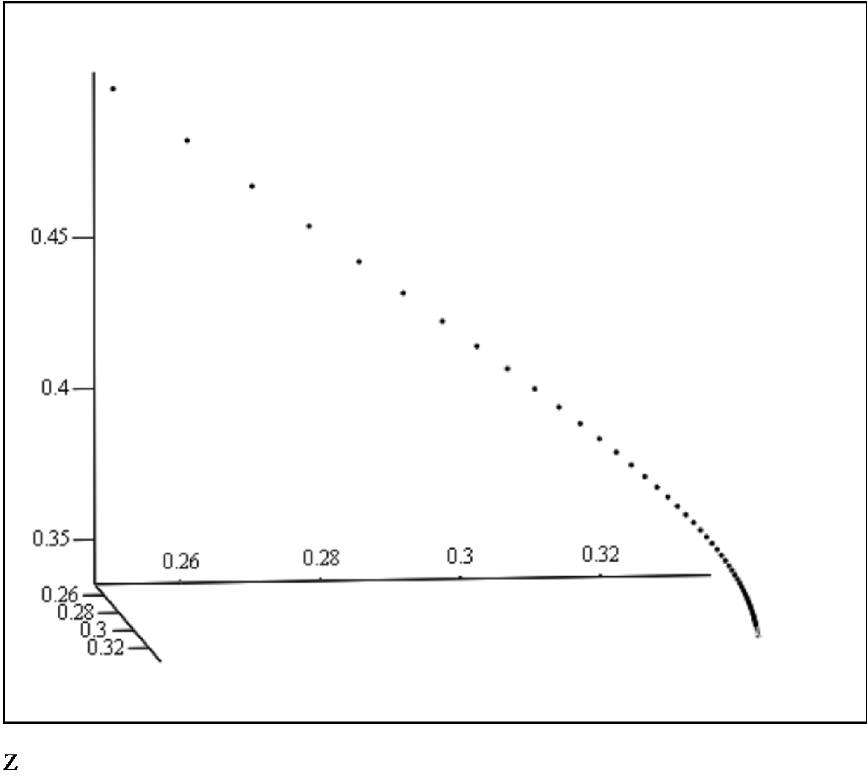
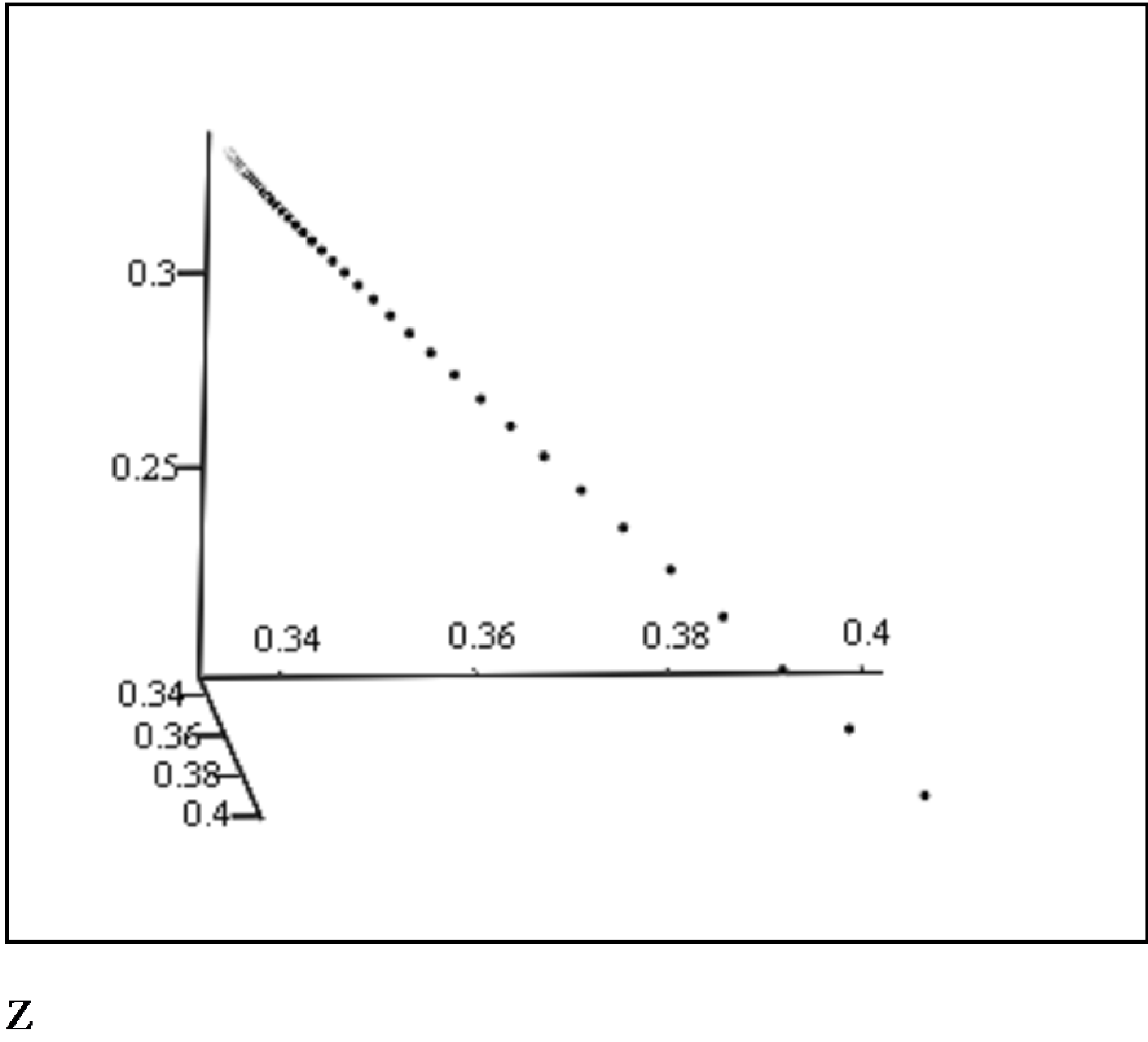
where For a fixed negative , formula (15) gives one solution located in the line . For a fixed positive , formula (15) defines two solutions, one of which, defined on the interval , is located in the half-plane , and the other, defined on the interval , is located in the half-plane . In addition to solutions located in these regions indicated above, equation (14) has two more solutions and which are formally obtained from (15) with and The phase portrait of equation (14) consists of five phase curves: two singular points 0 and , two rays and and an interval . Here, the point is stable, and the point is an unstable equilibrium. Taking into account, and , as above, we obtain that in this case i.e. the considered dynamical system is at rest. As mentioned above, we failed to find an analytical solution to the Cauchy problem for the system (1) in the general case. In this regard, with the help of the MathCAD program, solutions of the Cauchy problem for system (1) were found and the phase portrait of the trajectory (with an accuracy of 0.001) was compiled in fig. 1,2. The phase portrait of system (1) is as follows:
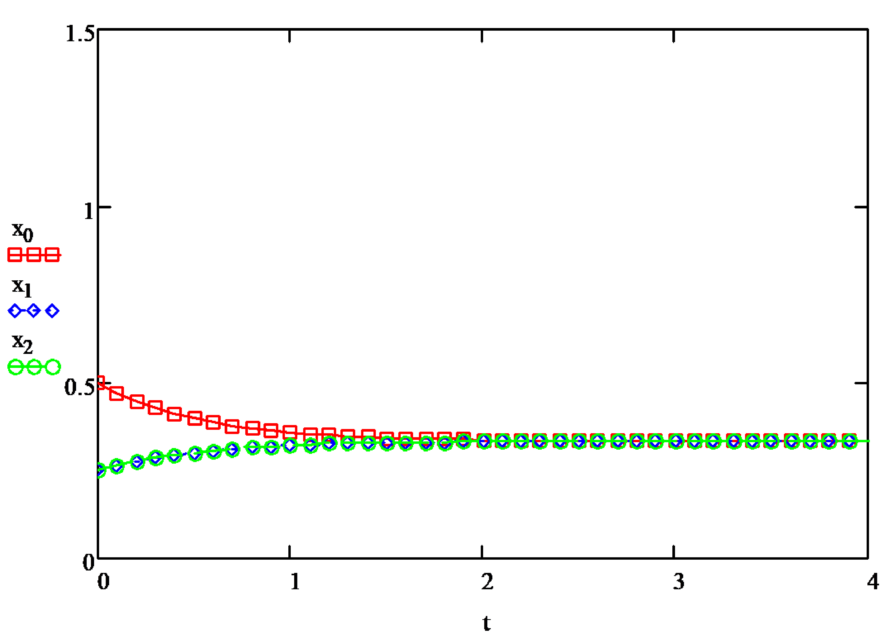
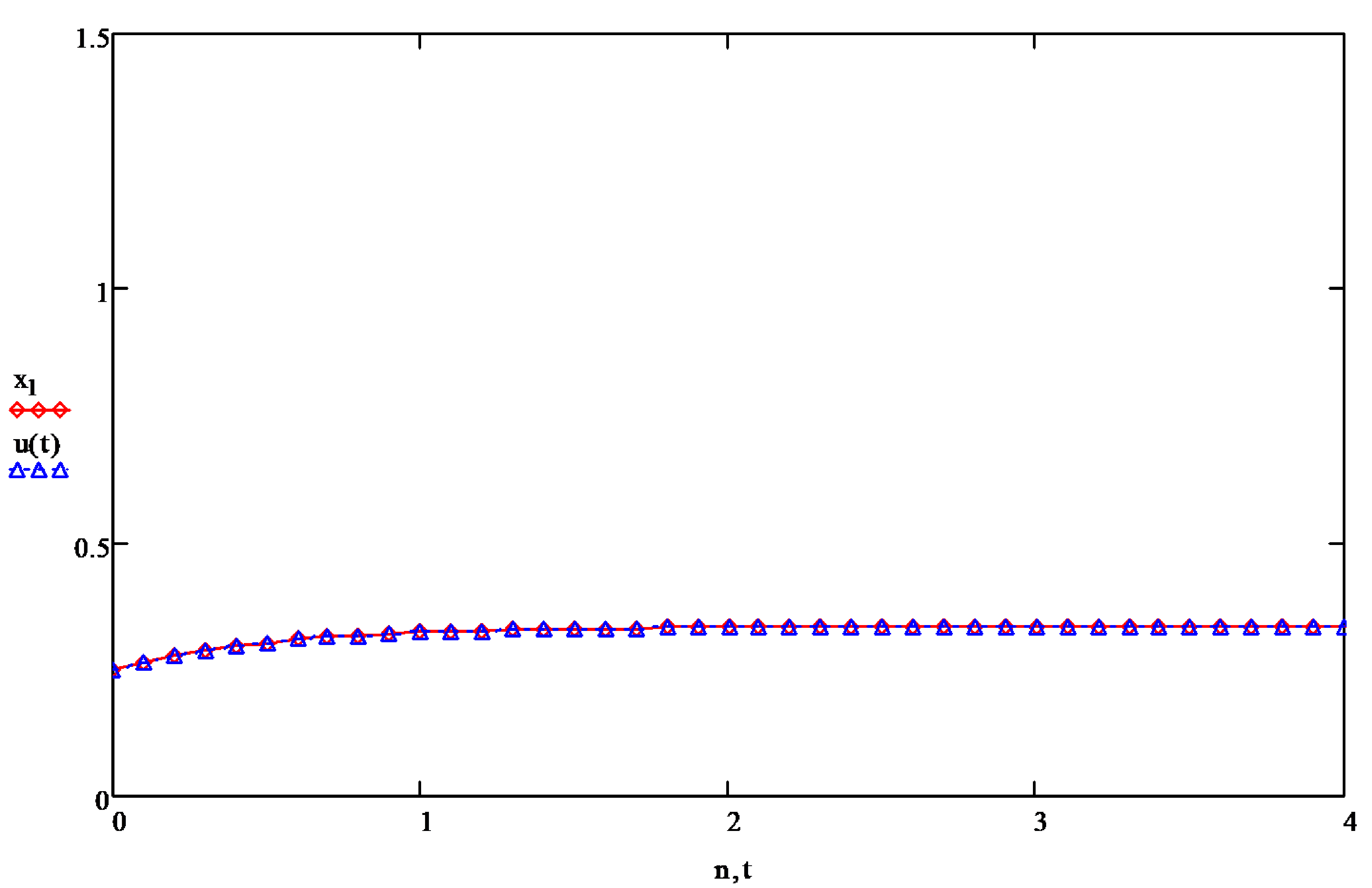
Also, for cases where and , and compared solutions of system (1), calculated using the MathCAD program with (12) and (13), respectively (fig. 3-6). To compare the numerical and analytical solutions (12) and (13) on the graph, we denote by numerical solutions, and by and analytic solutions from (12) and (13), respectively. As a result of the research, it was found that the difference between the numerical solutions (1) and (12), (13) does not exceed 0.001, and for , the numerical and analytical solutions almost coincide and together tend to the rest point .
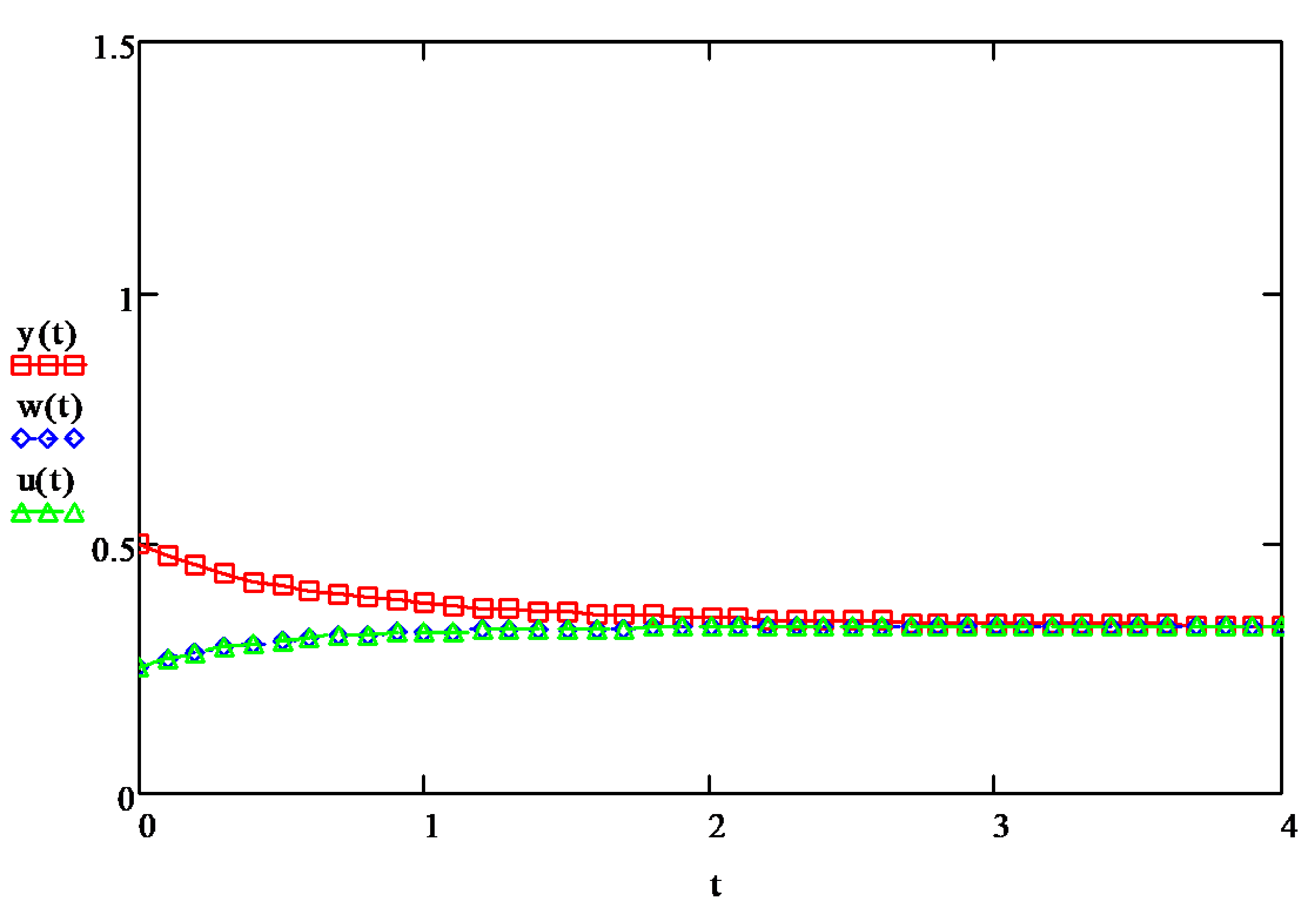

A similar picture takes place when comparing the solution of system (1) with analytical solutions (13) in the line , , , with the same initial conditions. Thereby, the following theorem has been proved. Theorem. System (1) with the conditions , , , and has a unique fixed point , which is a hyperbolic saddle. In addition, the solution (12) and (13) of system (10) exponentially tends to the solution of the system (1). The results of this paper show that the dynamics of an analogue of strictly non-Volterra operators with continuous time is much richer than the dynamics of non-Volterra operators with discrete time (see [Mukh15]). This is also seen from the phase portrait of system (1), which consists of five curves. It was found that tends to the equilibrium point according to formulas (12) and (13), and the sum tends to unity exponentially fast as . In addition, in the absence of conditions
the trajectory defined by system (1) in overall, has several curves. Each strictly non-Volterra quadratic operator is an interesting example in the theory of multidimensional nonlinear dynamical systems with various trajectory behavior. A comparative analysis of the results obtained in [Mukh15] and in the present paper shows that the equilibrium positions of system (1) coincide with the fixed point of the operator [Mukh15] only when , , and and both of these trajectories tend to the equilibrium position exponentially fast. In addition, we can say that considering an analog of a quadratic operator (studied in [Mukh15]) with continuous time gives some advantage. Since it has been established that on the basis of computer calculations it can be said that for solutions of system (1) obtained using MathCAD (more than 100 solutions with different initial values are calculated and compared) coincide with the solutions obtained analytically (12) and (13). The author thanks prof. U.A. Rozikov for useful discussions.
References
- [1] \referPaperAnge1 \RauthorAngelina M. L.,Melissa A.P.,Thomas S., Nakul Ch. \RtitleMathematical modeling of mosquito dispersal in a heterogeneous environment \RjournalMathematical Biosciences \Rvolume241 \Ryear2013 \Rpages198-216
- [2] \referPaperBern2 \RauthorBernshtein S. N. \RtitleSolution of one mathematical problem related to the theory of inheritance \RjournalScientific Notes of the Research Department of Ukraine. Department of Mathematics [in russian] \Ryear1924 \Rnumber1 \Rpages83-115
- [3] \referBookBrat3 \RauthorBratus A. S., Novozhilov A. S. and Platonov A. P. \RtitleDynamical systems and models of biology \RpublisherMoscow Fizmatlit [in russian] \Ryear2009 \Rpages400
- [4] \referPaperGani4 \RauthorGanikhodzhaev N. N. and Zanin D. V. \RtitleOn a necessary condition for the ergodicity of quadratic operators defined on the two-dimensional simplex \RjournalRussian Math. Surveys \Rvolume59 \Ryear2004 \Rnumber3 \Rpages571-572
- [5] \referPaperGani5 \RauthorGanikhodzhaev R. N. \RtitleQuadratic stochastic operators, Lyapunov functions, and tournaments \RjournalRussian Acad. Sci. Math. sb. [in russian] \Rvolume183 \Ryear1992 \Rnumber8 \Rpages119-140
- [6] \referPaperGani6 \RauthorGanikhodzhaev R. N. and Sarimsakov A. T. \RtitleMathematical model of the coalition of biological systems \RjournalDokl. AN UzSSR [in russian] \Ryear1992 \Rnumber3 \Rpages14-17
- [7] \referPaperGani7 \RauthorGanikhodzhaev R. N. \RtitleA family of quadratic stochastic operators, operating in S2 \RjournalDokl. AN UzSSR [in russian] \Ryear1989 \Rnumber1 \Rpages3-5
- [8] \referPaperGani8 \RauthorGanikhodzhaev R. N. and Eshmamatova D. B. \RtitleQuadratic automorphisms of a simplex and the asymptotic behavior of their trajectories \RjournalVladikavkaz. matem. zhurn., [in russian] \Rvolume8 \Ryear2006 \Rnumber2 \Rpages12-28
- [9] \referPaperGani9 \RauthorGanikhodzhaev R. N., Mukhamedov F. M. and Rozikov U. A. \RtitleQuadratic stochastic operators and processes: results and open problems \RjournalInf. Dim. Anal. Quant. Prob. Rel. Fields \Rvolume14 \Ryear2011 \Rnumber2 \Rpages279-335
- [10] \referPaperHuan10 \RauthorJicai Huang, Shigui Ruan and Jing Song \RtitleBifurcations in a predator-prey system of Leslie type with generalized Holling type III functional response \RjournalJ. Differential Equations \Ryear2014 \Rnumber257 \Rpages1721-1752
- [11] \referBookKamk11 \RauthorKamke E. \RtitleHandbook of ordinary differential equations. Moscow, publishing house \RpublisherMoscow, Nauka [in russian] \Ryear1976 \Rpages576
- [12] \referPaperKest12 \RauthorKesten H. \RtitleQuadratic transformations: a model for population growth \RjournalAdvances in Appl. Probability \Ryear1970 \Rnumber2 \Rpages1-82
- [13] \referBookLyub13 \RauthorLyubich Yu. I. \RtitleMathematical Structures in Population Genetics (Mathematics, 22) \RpublisherSpringer-Verlag, Berlin \Ryear1992 \Rpages383
- [14] \referPaperMukh14 \RauthorMukhamedov F. M. \RtitleInfinite-dimensional quadratic Volterra operators \RjournalRussian Math. Surveys \Rvolume55 \Ryear2000 \Rnumber6 \Rpages1161-1162
- [15] \referOtherMukh15 \RauthorMukhitdinov R. T. \RtitleOn a strictly non-Volterra quadratic operator. Abstracts of the international conference Operator algebras and quantum probability theory, University, Tashkent [in russian] \Ryear2005 \Rpages134-135
- [16] \referPaperRasu16 \RauthorRasulov Kh. R. \RtitleOn a continuous time F - quadratic dynamical system \RjournalUzbek mathematical journal \Ryear2018 \Rnumber4 \Rpages126-130
- [17] \referPaperRozi17 \RauthorRozikov U. A. and Zhamilov U. U. \RtitleThe dynamics of strictly non-Volterra quadratic stochastic operators on the 2-simplex \RjournalRussian Acad. Sci. Math. Sb. \Rvolume200 \Ryear2009 \Rnumber9 \Rpages1339-1351
- [18] \referPaperRozi18 \RauthorRozikov U. A. and Zhamilov U. U. \RtitleF-quadratic stochastic operators \RjournalMath. Notes \Rvolume83 \Ryear2008 \Rnumber4 \Rpages554-559
- [19] \referPaperTian19 \RauthorTianran Zhang, Wendi Wang \RtitleHopf bifurcation and bistability of a nutrient-phytoplankton-zooplankton model \RjournalApplied Mathematical Modeling \Rvolume36 \Ryear2012 \Rnumber12 \Rpages6225-6235
- [20] \referPaperTokm20 \RauthorTokmachev M. S. \RtitleAbel differential equations of the second kind \RjournalBulletin of Novgorod State University [in russian] \Ryear2002 \Rnumber22 \Rpages19-23
- [21] \referBookUlam21 \RauthorUlam S. M. \RtitleA collection of mathematical problems \RpublisherNew York-London, Interscience Publ. \Ryear1960 \Rpages150
- [22] \referBookZait22 \RauthorZaitsev V. F. and Polyanin A. D. \RtitleHandbook on ordinary differential equations \RpublisherMoscow, Fizmatlit house [in russian] \Ryear2001 \Rpages576
- [23]
December 13, 2020March 04, 2021Utkir Rozikov