Extended formulations via decision diagrams

Abstract

We propose a general algorithm of constructing an extended formulation for any given set of linear constraints with integer coefficients. Our algorithm consists of two phases: first construct a decision diagram $(V,E)$ that somehow represents a given $m\times n$ constraint matrix, and then build an equivalent set of $|E|$ linear constraints over $n+|V|$ variables. That is, the size of the resultant extended formulation depends not explicitly on the number $m$ of the original constraints, but on its decision diagram representation. Therefore, we may significantly reduce the computation time and space for optimization problems with integer constraint matrices by solving them under the extended formulations, especially when we obtain concise decision diagram representations for the matrices. Then, we consider the $1$-norm regularized soft margin optimization over the binary instance space $\{0,1\}^{n}$, a standard optimization problem in the machine learning literature. This problem is motivating since the naive application of our extended formulation produces decision diagrams of size $\Omega(m)$. For this problem, we give a modified formulation which works in practice and efficient algorithms whose time complexity depends on the size of the diagrams. This problem can be formulated as a linear programming problem with $m$ constraints with $\{-1,0,1\}$-valued coefficients over $n$ variables, where $m$ is the size of the given sample. We demonstrate the effectiveness of our extended formulations for mixed integer programming and the $1$-norm regularized soft margin optimization tasks over synthetic and real datasets.

Keywords Extend formulation  $\cdot$ Decision diagrams  $\cdot$ Mixed integer programs  $\cdot$ Soft margin optimization

1 Introduction

Large-scale optimization tasks appear in many areas such as machine learning, operations research, and engineering. Time/memory-efficient optimization techniques are more in demand than ever. Various approaches have been proposed to efficiently solve optimization problems over huge data, e.g., stochastic gradient descent methods (e.g.,Duchi et al. (2011)) and concurrent computing techniques using GPUs (e.g.,Raina et al. (2009)). Among them, we focus on the “computation on compressed data” approach, where we first compress the given data somehow and then employ an algorithm that works directly on the compressed data (i.e., without decompressing the data) to complete the task, in an attempt to reduce computation time and/or space. Algorithms on compressed data are mainly studied in string processing (e.g., Goto et al. (2013); Hermelin et al. (2009); Lifshits (2007); Lohrey (2012); Rytter (2004)), enumeration of combinatorial objects(e.g., Minato (2017)), and combinatorial optimization(e.g., Bergman et al. (2016)). In particular, in the work on combinatorial optimization, they compress the set of feasible solutions that satisfy given constraints into a decision diagram so that minimizing a linear objective can be done by finding the shortest path in the decision diagram. Although we can find the optimal solution very efficiently when the size of the decision diagram is small, the method can only be applied to specific types of discrete optimization problems where the feasible solution set is finite, and the objective function is linear.

Whereas, we mainly consider a more general form of discrete/continuous optimization problems that include linear constraints with integer coefficients:

$$\min_{\bm{x}\in X\subset\mathbb{R}^{n}}f(\bm{x})\quad\text{s.t.}\quad\bm{A}\bm{x}\geq\bm{b}$$ (1)

for some $\bm{A}\in C^{m\times n}$ and $\bm{b}\in C^{m}$, where $X$ denotes the constraints other than $\bm{A}\bm{x}\geq\bm{b}$, and $C$ is a finite subset of integers. This class of problems includes LP, QP, SDP, and MIP with linear constraints of integer coefficients. So our target problem is fairly general. Without loss of generality, we assume $m>n$, and we are particularly interested in the case where $m$ is huge.

In this paper, we propose a pre-processing method that "rewrites" integer-valued linear constraints with equivalent but more concise ones. More precisely, we propose a general algorithm that, when given an integer-valued constraint matrix $(\bm{A},\bm{b})\in C^{m\times n}\times C^{m}$ of an optimization problem (1), produces a matrix $(\bm{A}^{\prime},\bm{b}^{\prime})\in C^{m^{\prime}\times(n+n^{\prime})}\times C^{m^{\prime}}$ that represents its extended formulation, that is, it holds that

$$\exists\bm{s}\in\mathbb{R}^{n^{\prime}},\bm{A}^{\prime}\begin{bmatrix}\bm{x}\\ \bm{s}\end{bmatrix}\geq\bm{b}^{\prime}\Leftrightarrow\bm{A}\bm{x}\geq\bm{b}$$

for some $n^{\prime}$ and $m^{\prime}$, with the hope that the size of $(\bm{A}^{\prime},\bm{b}^{\prime})$ is much smaller than that of $(\bm{A},\bm{b})$ even at the cost of adding $n^{\prime}$ extra variables. Using the extended formulation, we obtain an equivalent optimization problem to (1):

$$\min_{\bm{x}\in X\subset\mathbb{R}^{n},\bm{s}\in\mathbb{R}^{n^{\prime}}}f(\bm{x})\quad\text{s.t.}\quad\bm{A}^{\prime}\begin{bmatrix}\bm{x}\\ \bm{s}\end{bmatrix}\geq\bm{b}^{\prime}.$$ (2)

Then, we can apply any existing generic solvers, e.g., MIP/QP/LP solvers if $f$ is linear or quadratic, to (2), combined with our pre-processing method, which may significantly reduce the computation time/space than applying them to the original problem (1).

To obtain a matrix $(\bm{A}^{\prime},\bm{b}^{\prime})$, we first construct a variant of a decision diagram called a Non-Deterministic Zero-Suppressed Decision Diagram (NZDD, for short) Fujita et al. (2020) that somehow represents the matrix $(\bm{A},\bm{b})$. Observing that the constraint $\bm{A}\bm{z}\geq\bm{b}$ can be restated in terms of the NZDD constructed as “every path length is lower bounded by 0” for an appropriate edge weighting, we establish the extended formulation $(\bm{A}^{\prime},\bm{b}^{\prime})\in C^{m^{\prime}\times(n+n^{\prime})}\times C^{m^{\prime}}$ with $m^{\prime}=|E|$ and $n^{\prime}=|V|$, where $V$ and $E$ are the sets of vertices and edges of the NZDD, respectively. One of the advantages of the result is that the size of the resulting optimization problem depends only on the size of the NZDD and the number $n$ of variables, but not on the number $m$ of the constraints in the original problem. Therefore, if the matrix $(\bm{A},\bm{b})$ is well compressed into a small NZDD, then we obtain an equivalent but concise optimization problem (2).

To clarify the differences between our work and previous work regarding optimization using decision diagrams, we summarize the characteristics of both results in Table 1. Notable differences are that (i) ours can treat optimization problems with any types of variables (discrete, or real), any types of objectives (including linear ones) but with integer coefficients on linear constraints, and (ii) ours uses decision diagrams for representing linear constraints while previous work uses them for representing feasible solutions of particular classes of problems. So, for particular classes of discrete optimization problems, the previous approach would work better with specific construction methods for decision diagrams. On the other hand, ours is suitable for continuous optimization problems or/and discrete optimization problems for which efficient construction methods for decision diagrams representing feasible solutions are not known. See the later section for more detailed descriptions of related work.

Table 1: Characteristics of previous work on optimization with decision diagrams (DDs) and ours.

	coeff. of lin. consts.	variables	objectives	DDs
Previous work	any type	binary/integer	linear	feasible solutions
Ours	binary/integer	any type	any type	lin. consts.

Among various linear optimization problems, we consider the $1$-norm regularized soft margin optimization as a non-trivial application of our method. This problem is a standard optimization problem in the machine learning literature, categorized as LP, for finding sparse linear classifiers given labeled instances. This problem is motivating and challenging in that it has $n+m$ variables and $m$ linear constraints, so the naive application of our method will not be successful as the size of the NZDD representing the constraints is $\Omega(m)$. For this problem, we propose a modified formulation that suffices to work well in practice, and we show efficient algorithms whose time complexity depends only on the size of the NZDD for the modified problem.

Furthermore, to realize succinct extended formulations, we propose practical heuristics for constructing NZDDs, which is our third contribution. Since it is not known to construct an NZDD of small size, we first construct a ZDD of minimal size, where the ZDD is a restricted form of the NZDD representation. To this end, we use a ZDD compression software called zcomp Toda (2013). Then, we give rewriting rules for NZDDs that reduce both the numbers of vertices and edges, and apply them to obtain NZDDs of smaller size of $V$ and $E$. Although the rules may increase the size of NZDDs (i.e., the total number of edge labels), the rules seem to work effectively since reducing $|V|$ and $|E|$ is more important for our purpose.

Experimental results on synthetic and real data sets show that our algorithms improve time/space efficiency significantly, especially when (i) $m\gg n$, and (ii) the set $C$ of integer coefficients is small, e.g., binary, where the datasets tend to have concise NZDD representations.

2 Related work

Various computational tasks over compressed strings or texts are investigated in algorithms and data mining literature, including, e.g., pattern matching over strings and computing edit distances or $q$-grams  Goto et al. (2013); Hermelin et al. (2009); Lifshits (2007); Lohrey (2012); Rytter (2004). The common assumption is that strings are compressed using the straight-line program, which is a class of context-free grammars generating only one string (e.g., LZ77 and +LZ78). As notable applications of string compression techniques to data mining and machine learning, Nishino et al. Nishino et al. (2014) and Tabei et al. Tabei et al. (2016) reduce the space complexity of matrix-based computations. So far, however, string compression-based approaches do not seem to be useful for representing linear constraints.

Decision diagrams are used in the enumeration of combinatorial objects, discrete optimization and so on. In short, a decision diagram is a directed acyclic graph with a root and a leaf, representing a subset family of some finite ground set $\Sigma$ or, equivalently, a boolean function. Each root-to-leaf path represents a set in the set family. The Binary Decision Diagram (BDD)Bryant (1986); Knuth (2011) and its variant, the Zero-Suppressed Binary Decision Diagram (ZDD)Knuth (2011); Minato (1993), are popular in the literature. These support various set operations (such as intersection and union) in efficient ways. Thanks to the DAG structure, linear optimization problems over combinatorial sets $X\subset\{0,1\}^{n}$ can be reduced to shortest/longest path problems over the diagrams representing $X$. This reduction is used to solve the exact optimization of NP-hard combinatorial problems (see, e.g., Bergman et al. (2016, 2011); Castro et al. (2019); Inoue et al. (2014); Morrison et al. (2016)) and enumeration tasks Minato (2017); Minato and Uno (2010); Minato et al. (2008). Among work on decision diagrams, the work of Fujita et al.Fujita et al. (2020) would be closest to ours. They propose a variant of ZDD called the Non-deterministic ZDD (NZDD) to represent labeled instances and show how to emulate the boosting algorithm AdaBoost^∗Rätsch and Warmuth (2005), a variant of AdaBoostFreund and Schapire (1997) that maximizes the margin, over NZDDs. We follow their NZDD-based representation of the data. But our work is different from Fujita et al. in that, they propose specific algorithms running over NZDDs, whereas our work presents extended formulations based on NZDDs, which could be used with various algorithms.

The notion of extended formulation arises in combinatorial optimization (e.g., Conforti et al. (2010); Yannakakis (1991)). The idea is to re-formulate a combinatorial optimization with an equivalent different form, so that the size of the problem is reduced. For example, a typical NP-hard combinatorial optimization problem has an integer programming formulation of exponential size. Then a good extended formulation should have a smaller size than the exponential. Typical work on extended formulation focuses on some characterization of the problem to obtain succinct formulations (see, e.g., Fiorini et al. (2021)). Our work is different from these in that we focus on the redundancy of the data and try to obtain succinct extended formulations for optimization problems described with data.

3 Preliminaries

The non-deterministic Zero-suppressed Decision Diagram (NZDD) Fujita et al. (2020) is a variant of the Zero-suppressed Decision Diagram(ZDD) Minato (1993); Knuth (2011) , representing subsets of some finite ground set $\Sigma$. More formally, NZDD is defined as follows.

Definition 1 (NZDD).

An NZDD $G$ is a tuple $G=(V,E,\Sigma,\Phi)$, where $(V,E)$ is a directed acyclic graph ($V$ and $E$ are the sets of nodes and edges, respectively) with a single root with no-incoming edges and a leaf with no outgoing edges, $\Sigma$ is the ground set, and $\Phi:E\to 2^{\Sigma}$ is a function assigning each edge $e$ a subset $\Phi(e)$ of $\Sigma$. More precisely, we allow $(V,E)$ to be a multigraph, i.e., two nodes can be connected with more than one edge.

Furthermore, an NZDD $G$ satisfies the following additional conditions. Let $\mathcal{P}_{G}$ be the set of paths in $G$ starting from the root to the leaf, where each path $P\in\mathcal{P}_{G}$ is represented as a subset of $E$, and for any path $P\in\mathcal{P}_{G}$, we abuse the notation and let $\Phi(P)=\cup_{e\in P}\Phi(e)$.

1. For any path $P\in\mathcal{P}_{G}$ and any edges $e,e^{\prime}\in P$, $\Phi(e)\cap\Phi(e^{\prime})=\emptyset$. That is, for any path $P$, an element $a\in\Sigma$ appears at most once in $P$.

2. For any paths $P,P^{\prime}\in\mathcal{P}_{G}$, $\Phi(P)\neq\Phi(P^{\prime})$. Thus, each path $P$ represents a different subset of $\Sigma$.

Then, an NZDD $G$ naturally corresponds to a subset family of $\Sigma$. Formally, let $L(G)=\{\Phi(P)\mid P\in\mathcal{P}_{G}\}$. Figure 1 illustrates an NZDD representing a subset family $\{\{a,b,c\},\{b\},\{b,c,d\},\{c,d\}\}$.

Figure 1: An NZDD representing $\{\{a,b,c\},\{b\},\{b,c,d\},\{c,d\}\}$.

A ZDD Minato (1993); Knuth (2011) can be viewed as a special form of NZDD $G=(V,E,\Sigma,\Phi)$ satisfying the following properties: (i) For each edge $e\in E$, $\Phi(e)=\{a\}$ for some $a\in\Sigma$ or $\Phi(e)=\emptyset$. (ii) Each internal node has at most two outgoing edges. If there are two edges, one is labeled with $\{a\}$ for some $a\in\Sigma$ and the other is labeled with $\emptyset$. (iii) There is a total order over $\Sigma$ such that, for any path $P\in\mathcal{P}_{G}$ and for any $e,e^{\prime}\in P$ labeled with singletons $\{a\}$ and $\{a^{\prime}\}$ respectively, if $e$ is an ancestor of $e^{\prime}$, $a$ precedes $a^{\prime}$ in the order.

We believe that that constructing a minimal NZDD for a given subset family is NP-hard since closely related problems are NP-hard. For example, constructing a minimal ZDD (over all orderings of $\Sigma$) is known to be NP-hard Knuth (2011), and construction of a minimal NFA which is equivalent to a given DFA is P-space hard Jiang and Ravikumar (1993). On the other hand, there is a practical construction algorithm of ZDDs given a subset family and a fixed order over $\Sigma$ using multi-key quicksort Toda (2013).

4 NZDDs for linear constraints with binary coefficients

In this section, we show an NZDD representation for linear constraints in problem (1) when linear constraints have $\{0,1\}$-valued coefficients, that is, $C=\{0,1\}$. We will discuss its extensions to integer coefficients in the later section. Let $\bm{a}_{i}\in\{0,1\}^{n}$ be the vector corresponding to the $i$-th row of the matrix $A\in\{0,1\}^{m\times n}$ (for $i\in[m]$). For $\bm{x}\in\{0,1\}^{n}$, let $\mathrm{idx}(\bm{x})=\{j\in[n]\mid x_{j}\neq 0\}$, i.e., the set of indices of nonzero components of $\bm{x}$. Then, we define $I=\{\mathrm{idx}(\bm{c}_{i})\mid\bm{c}_{i}=(\bm{a}_{i},b_{i}),i\in[m]\}$. Note that $I$ is a subset family of $2^{[n+1]}$. Then we assume that we have some NZDD $G=(V,E,[n+1],\Phi)$ representing $I$, that is, $L(G)=I$. We will later show how to construct NZDDs.

The following theorem shows the equivalence between the original problem (1) and a problem described with the NZDD $G$.

Theorem 1.

Let $G=(V,E,[n+1],\Phi)$ be an NZDD such that $L(G)=I$. Then the following optimization problem is equivalent to problem (1):

$$\min_{\bm{x}\in X\subset\mathbb{R}^{n},\bm{s}\in\mathbb{R}^{|V|}} f(\bm{x})$$ (3)

s.t. $$s_{e.u}+\sum_{j\in\Phi(e)}x^{\prime}_{j}\geq s_{e.v},\quad\forall e\in E,$$

$$s_{\mathrm{root}}=0,~{}s_{\mathrm{leaf}}=0,$$

$$\bm{x}^{\prime}=(\bm{x},-1),$$

where $e.u$ and $e.v$ are nodes that the edge $e$ is directed from and to, respectively.

Before going through the proof, let us explain some intuition on problem (3). Intuitively, each linear constraint in (1) is encoded as a path from the root to the leaf in the NZDD $G$, and a new variable $s_{v}$ for each node $v$ represents a lower bound of the length of the shortest path from the root to $v$. The inequalities in (3) reflect the structure of the standard dynamic programming of Dijkstra, so that all inequalities are satisfied if and only if the length of all paths is larger than zero. In Figure 2, we show an illustration of the extended formulation.

Proof.

Let $\bm{x}_{\star}$ and $(\hat{\bm{x}}^{\prime},\hat{\bm{s}})$ be the optimal solutions of problems (1) and (3), respectively. It suffices to show that each optimal solution can construct a feasible solution of the other problem.

Let $\hat{\bm{x}}$ be the vector consisting of the first $n$ components of $\hat{\bm{x}}^{\prime}$. For each constraint $\bm{a}_{i}^{\top}\bm{x}\geq b_{i}$ ($i\in[m]$) in problem (1), there exists the corresponding path $P_{i}\in\mathcal{P}_{G}$. By repeatedly applying the first constraint in (3 along the path $P_{i}$, we have $\sum_{e\in P_{i}}\sum_{j\in\Phi(e)}\hat{z}_{j}^{\prime}\geq\hat{s}_{\mathrm{leaf}}=0$. Further, since $\Phi(P_{i})$ represents the set of indices of nonzero components of $\bm{c}_{i}$, $\sum_{e\in P_{i}}\sum_{j\in\Phi(e)}\hat{z}_{j}^{\prime}=\bm{c}_{i}^{\top}\hat{\bm{x}}^{\prime}=\bm{a}_{i}^{\top}\hat{\bm{x}}-b_{i}$. By combining these inequalities, we have $\bm{a}_{i}^{\top}\hat{\bm{x}}-b_{i}\geq 0$. This implies that $\hat{\bm{x}}$ is a feasible solution of (1) and thus $f(\bm{x}_{\star})\leq f(\hat{\bm{x}})$.

Let $\bm{x}_{\star}^{\prime}=(\bm{x}_{\star},-1)$. Assuming a topological order on $V$(from the root to the leaf), we define $s_{\star,\mathrm{root}}=s_{\star,\mathrm{leaf}}=0$ and $s_{\star,v}=\min_{e\in E,e.v=v}s_{\star,e.u}+\sum_{j\in\Phi(e)}z_{\star,j}^{\prime}$ for each $v\in V\setminus\{\mathrm{root},\mathrm{leaf}\}$. Then, we have, for each $e\in E$ s.t. $e.v\neq\mathrm{leaf}$, $s_{\star,e.v}\leq s_{\star,e.u}+\sum_{j\in\Phi(e)}z_{\star,j}^{\prime}$ by definition. Now, $\min_{e\in E,e.v=\mathrm{leaf}}s_{\star,e.u}+\sum_{j\in\Phi(e)}z_{\star,j}^{\prime}$ is achieved by a path $P\in\mathcal{P}_{G}$ corresponding to $\arg\min_{i\in[m]}\bm{a}_{i}^{\top}\bm{x}_{\star}-b_{i}$, which is $\geq 0$ since $\bm{x}_{\star}$ is feasible w.r.t. (1). Therefore, $s_{\star,e.v}\leq s_{\star,e.u}+\sum_{j\in\Phi(e)}z_{\star,j}^{\prime}$ for $e\in E$ s.t. $e.v=\mathrm{leaf}$ as well. Thus, $(\bm{x}_{\star}^{\prime},s_{\star})$ is a feasible solution of (3) and $f(\hat{\bm{x}})\leq f(\bm{x}_{\star})$. ∎

Figure 2: An illustration of the extended formulation. Left: Original constraints as in (1). Middle: A NZDD representation of the left constraints. Right: The matrix form (3) of the middle diagram without constant terms. This example reduces the $13$ constraints to $9$ constraints by adding $2$ variables.

Given the NZDD $G=(V,E)$, problem (3) contains $n+|V|$ variables and $|E|$ linear constraints, where $|V|$ variables are real. In particular, if problem (1) is LP or IP, then problem (3) is LP, or MIP, respectively.

5 Extensions to integer coefficients

We briefly discuss how to extend our NZDD representation of linear constraints to the cases where coefficients of linear constraints belong to a finite set $C$ of integers. There are two ways to do so.

Binary encoding of integers

We assume some encoding of integers in $C$ with $O(\log|C|)$ bits. Then, each bit can be viewed as a binary-valued variable. Each integer coefficient can be also recovered with its binary representation. Under this attempt, the resulting extended formulation has $O(n\log|C|+|V|)$ variables and $O(|E|)$ linear constraints.

Extending $\Sigma$

Another attempt is to extend the domain $\Sigma$ of an NZDD $G=(V,E,\Sigma,\Phi)$. The extended domain $\Sigma^{\prime}$ consists of all pairs of integers in $C$ and elements in $\Sigma$. Again, integer coefficients are recovered through the new domain $\Sigma^{\prime}$. The resulting extended formulation has $O(n|C|+|V|)$ variables and $O(|E|)$ linear constraints. While the size of the problem is larger than the binary encoding, its implementation is easy in practice and could be effective for $C$ of small size.

6 $1$-norm regularized soft margin optimization

The $1$-norm regularized soft margin optimization is a standard linear programming formulation of finding a sparse linear classifier with large margin (see, e.g., Demiriz et al. (2002); Warmuth et al. (2007, 2008)). We are given a sequence $S$ of labeled instances $S=((\bm{x}_{1},y_{1}),\dots,(\bm{x}_{m},y_{m}))\in(\mathcal{X}\times\{-1,1\})^{m}$, where $\mathcal{X}\subset\mathbb{R}^{n}$ is the set of instances. For clarity, we assume that the domain is the set of binary vectors, i.e., $\mathcal{X}=\{0,1\}^{n}$. This is common in many applications when we employ the bag-of-words representation of instances. Given a parameter $\nu\in(0,1]$ and a sequence $S$ of labeled instances, the $1$-norm regularized soft margin optimization is defined as follows :

$$\max_{\rho,\bm{w},b,\bm{\xi}} \quad\rho-\frac{1}{\nu m}\sum_{i=1}^{m}\xi_{i}$$ (4)

s.t. $$\quad y_{i}(\bm{w}^{\top}\bm{x}_{i}-b)\geq\rho-\xi_{i}\quad\forall i=1,\dots,m,$$

$$\quad\sum_{j}w_{j}+b=1,\bm{w}\in\mathbb{R}^{n}_{+},b\geq 0,\bm{\xi}\in\mathbb{R}^{m}_{+}.$$

For the parameter $\nu\in(0,1]$ and the optimal solution $(\rho^{\star},\bm{w}^{\star},b^{\star},\bm{\xi}^{\star})$, by a duality argument, it can be verified that there are at least $(1-\nu)m$ instances that has margin larger than $\rho^{\star}$, i.e., $y_{i}(\bm{w}^{\star\top}\bm{x}_{i}-b^{\star})\geq\rho^{\star}$ Demiriz et al. (2002).

We formulate a variant of the $1$-norm reguralized soft margin optimization based on NZDDs and propose efficient algorithms. Our generic re-formulation of (3) can be applied to the soft margin problem (4) as well. However, a direct application is not successful since problem (4) contains $O(m)$ slack variables $\bm{\xi}$ and each $\xi_{i}$ appears only once in $m$ linear constraints. That implies a resulting NZDD contains $\Omega(m)$ edges. Therefore, we are motivated to formulate a soft margin optimization for which a succinct NZDD representation exists.

Our basic idea is as follows: Suppose that we have some NZDD $G=(V,E,\Phi,\Sigma)$ such that each path $P$ corresponds to a constraint $y_{i}(\bm{w}^{\top}\bm{x}_{i}+b)\geq\rho$. Our idea is to introduce a slack variable $\beta_{e}$ on each edge $e$ along the path $P$, instead of using a slack variable $\xi_{i}$ for each instance $i\in[m]$.

Given some NZDD $G=(V,E,\Sigma,\Phi)$,

$$\max_{\rho,b,\bm{w},\bm{\beta}}\quad \rho-\frac{1}{\nu m}\sum_{i=1}^{m}\sum_{e\in P_{i}}\beta_{e}$$ (5)

s.t. $$y_{i}(\bm{w}^{\top}\bm{x}_{i}-b)\geq\rho-\sum_{e\in P_{i}}\beta_{e},\;\forall i=1,\dots,m,$$

$$\sum_{j=1}^{n}w_{j}+b=1,\quad b\geq 0,\bm{w}\in\mathbb{R}^{n}_{+},\bm{\beta}\in\mathbb{R}^{E}_{+}.$$

Note that, the sum of the slack variables $\sum_{e\in P_{i}}\beta_{e}$ for each instance $\bm{x}_{i}$ is more restricted than the original slack variable $\xi_{i}$. This observation implies the following.

Proposition 1.

An optimal solution of problem (5) is a feasible solution of problem (4).

Although problem (5) is a restricted version of (4), we observe that this restriction does not decrease the generalization ability in our experiments, which is shown later.

Now we introduce an equivalent formulation of (5) which is fully described with an NZDD. To do so, we specify how to construct the input NZDD as follows.

NZDD $G$ representing the sample $S$

Let $I^{+}=\{\mathrm{idx}((\bm{x}_{i},1))\in 2^{[n+1]}\mid y_{i}=1,i\in[m]\}$ and $I^{-}=\{\mathrm{idx}((\bm{x}_{i},1))\in 2^{[n+1]}\mid y_{i}=-1,i\in[m]\}$ be the set families of indices of nonzero components of positive and negative instances, respectively. For $I^{+}$ and $I^{-}$, let $G^{+}=(V^{+},E^{+},[n+1],\Phi^{+})$ and $G^{-}=(V^{-},E^{-},[n+1],\Phi^{-})$, be corresponding NZDDs such that $L(G^{+})=I^{+}$ and $L(G^{-})=I^{-}$, respectively. Finally, we connect $G^{+}$ and $G^{-}$ in parallel; We denote the resulting NZDD as $G=(V,E,[n+1],\Phi)$, where $V=V^{+}\cup V^{-}\cup\{\mathrm{root},\mathrm{leaf}\}\setminus\{\mathrm{leaf}^{+},\mathrm{leaf}^{-}\}$ and $E=E^{+}\cup E^{-}\cup\{(\mathrm{root},\mathrm{root}^{+}),(\mathrm{root},\mathrm{root}^{-})\}$, such that (i) two leaf nodes $\mathrm{leaf}^{+},\mathrm{leaf}^{-}$ of $G^{+}$ and $G^{-}$ are merged into a new leaf node $\mathrm{leaf}$, (ii) there are two edges $e$ from a new root node $\mathrm{root}$ to root nodes of $G^{+}$ and $G^{-}$ with $\Phi(e)=\emptyset$, and (iii) for other edges $e\in E$, $\Phi(e)=\Phi^{+}(e)$ if $e\in E^{+}$ and $\Phi(e)=\Phi^{-}(e)$ if $e\in E^{-}$.

$$\max_{\rho,\bm{w},\bm{\beta},\bm{s}} \quad\rho-\frac{1}{\nu m}\sum_{e\in E}m_{e}\beta_{e}$$ (6)

s.t. $$s_{e.u}+\mathrm{sign}(e)\sum_{j\in\Phi(e)}w_{j}+\beta_{e}\geq s_{e.v},\quad\forall e\in E,$$

$$s_{\mathrm{root}}=0,~{}s_{\mathrm{leaf}}\geq\rho,$$

$$\sum_{j=1}^{n}w_{j}-w_{n+1}=1,$$

$$w_{j}\geq 0,\;i\in[n],w_{n+1}\leq 0,\bm{\beta}\geq\bm{0},$$

where $m_{e}$ is the number of paths going thorough the edge $e$, and $\mathrm{sign}(e)$ is defined as $\mathrm{sign}(e)=-1$ if $e\in E^{-}$ and $\mathrm{sign}(e)=1$, otherwise. The constants $m_{e}$ can be computed in time $O(|E|)$ a priori by a dynamic programming over $G$. Note that the bias term $-b$ correspond to $w_{n+1}$ for notatinal convenience. Then, by following the same proof argument of Theorem 1, we have the following corollary.

Corollary 1.

Problem (6) is equivalent to problem (5) .

Problem (6) has $O(n+|V|+|E|)$ variables and $O(|E|)$ linear constraints, whereas the original formulation (4) has $O(n+m)$ variables and $O(m)$ linear constraints. So, with a concise NZDD representation of the sample, we obtain an extended formulation whose size is independent of $m$ of the sample size. In later subsections, we propose two efficient solving methods for problem (6).

6.1 Column Generation

Algorithm 1 Column Generation

0:  NZDD $G=(V,E,\Sigma,\Phi)$.

1:  Let $\bm{d}_{1}\in[0,1]^{|E|}$ be any vector satisfying (9), (10), and (11). Let $J_{0}=\emptyset$.

2:  for $t=1,2,...$ do

3:     Let $j_{t}=\arg\max_{j\in[n+1]}\mathrm{sign}(j)\sum_{e:j\in\Phi(e)}\mathrm{sign}(e)d_{e}$ and let $\hat{\gamma}_{t}$ be its objective value.

4:     If $\hat{\gamma}_{t}\leq\gamma_{t}+\varepsilon$, let $T=t-1$ and break.

5:     Let $J_{t}=J_{t-1}\cup\{j_{t}\}$ and update $(\bm{d}_{t+1},\gamma_{t+1})$ as:

$$\min_{\bm{d},\gamma} \gamma$$ (7)

s.t. $$\mathrm{sign}(j)\sum_{e:j\in\Phi(e)}\mathrm{sign}(e)d_{e}\leq\gamma,\forall j\in J_{t},$$

$$\text{constraints (\ref{const:d1}), (\ref{const:d2}), and (\ref{const:d3})}.$$

6:  end for

6:  Output the Lagrangian coefficients $(\bm{w}_{T},\bm{\beta}_{T},\rho_{T})$ for the subproblem w.r.t. $J_{T}$.

In this subsection, we propose a column generation-based method for solving the modified $1$-norm soft margin optimization problem (6). Although the size of the extended formulation (6) does not depend on the size of linear constraints $m$ of the original problem, it still depends on $n$, the size of variables. The column generation is a standard approach of linear programming that tries to reduce either the size of linear constraints/variables by solving smaller subproblems. In our case, we try to avoid problems depending on the size of variables $n$.

By a standard dual argument of linear programming, the equivalent dual problem of (6) is given as follows.

$$\min_{\gamma,\bm{d}}\gamma$$ (8)

s.t. $$\mathrm{sign}(j)\sum_{e:j\in\Phi(e)}\mathrm{sign}(e)d_{e}\leq\gamma\quad(j\in[n+1])$$

$$\sum_{e:e.u=u}d_{e}=\sum_{e:e.v=u}d_{e},\;\forall u\in V\setminus\{\mathrm{root},\mathrm{leaf}\},$$ (9)

$$\sum_{e:e.u=\mathrm{root}}d_{e}=1,\sum_{e:e.v=\mathrm{leaf}}d_{e}=1,$$ (10)

$$0\leq d_{e}\leq\frac{m_{e}}{\nu m}\quad(e\in E),$$ (11)

where $\mathrm{sign}(j)=1$ for $j\in[n]$ and $sign(j)=-1$ for $j=n+1$. Here, the dual problem (6) has $|E|+1$ variables and $n$ linear constraints. Roughly speaking, this problem is to find a vector $\bm{d}$ that represents a “flow” from the root to the leaf in the NZDD optimizing some objective, where the total flow is $1$. The objective is $\gamma$, the upper bound of $\mathrm{sign}(j)\sum_{e:j\in\Phi(e)}\mathrm{sign}(e)d_{e}$ for each $j\in[n+1]$. The column generation-based algorithm is given in Algorithm 1. The algorithm repeatedly solves the subproblems whose constraints related to $\gamma$ are only restricted to a subset $J_{t}\subseteq[n+1]$. Then it adds $j_{t+1}$ to $J_{t}$ (updated as $J_{t+1}$), where $j_{t+1}$ corresponds to the constraint that violates condition (9) the most with respect to the current solution $(\gamma_{t},\bm{d}_{t})$. It can be shown that the column-generation algorithm finds an $\varepsilon$-approximate solution.

Theorem 2.

Algorithm 1 outputs an $\varepsilon$-approximate solution of (6).

Proof.

Let $(\bm{d}^{\star},\gamma^{\star})$ be an optimal solution of (8) and let $\pi^{\star}$ and $\pi_{T}$ be the optimum of (6) and the primal one of the dual subproblem for $T$, respectively. By the duality, we have $\gamma_{T}=\pi_{T}$ and $\gamma^{\star}=\pi^{\star}$. We show that $\pi_{T}\geq\pi^{\star}-\varepsilon$. By definition of $T$, for any $j\in[n+1]\setminus J_{T}$, $\mathrm{sign}(j)\sum_{e:j\in\Phi(e)}\mathrm{sign}(e)d_{e}\leq\hat{\gamma}_{T+1}\leq\gamma_{T+1}+\varepsilon$. Then, $(\bm{d}_{T+1},\gamma_{T+1}+\varepsilon)$ is a feasible solution of (8). So, $\mathrm{sign}(j_{T+1})\sum_{e:j\in\Phi(e)}\mathrm{sign}(e)d_{e}=\hat{\gamma}_{T+1}\geq\gamma^{\star}$. Combining these observations, $\pi_{T}=\gamma_{T}\geq\gamma^{\star}-\varepsilon=\pi^{\star}-\varepsilon$ as claimed. ∎

As for its time complexity analysis, similar to other column generation techniques, we do not have non-trivial iteration bounds. In the next section, we propose another algorithm with theoretical guarantee of an iteration bound.

6.2 Performing ERLPBoost over an NZDD

We can emulate ERLPBoost Warmuth et al. (2008) on an NZDD. The algorithm is the same as ERLPBoost except for the update rule. Let $d^{0}_{e}=\frac{m_{e}}{m}$ for all $e\in E$. In each iteration $t$, the compressed version of ERLPBoost solves the following sub-problem:

$$\min_{\gamma,\boldsymbol{d}}\quad \gamma+\frac{1}{\eta}\left[\sum_{e\in E}d_{e}\ln\frac{d_{e}}{d^{0}_{e}}-d_{e}+d^{0}_{e}\right]$$ (12)

s.t. $$\mathrm{sign}(j)\sum_{e:j\in\Phi(e)}\mathrm{sign}(e)d_{e}\leq\gamma,\quad\forall j\in J_{t},$$

$$\text{constraints~{}(\ref{const:d1}), (\ref{const:d2}), and~{}(\ref{const:d3})}.$$

Here, $\eta>0$ is some parameter. One can rewrite (12) in terms of $\bm{d}$ by introducing $\max$ function. We denote the resulting objective function as $P^{t}(\bm{d})$. Algorithm 2 shows ERLPBoost over an NZDD.

Algorithm 2 ERLPBoost over an NZDD

0:  NZDD $G=(V,E,\Sigma,\Phi)$

1:  Set $d^{0}_{e}=\frac{m_{e}}{m}$ for all $e\in E$. Let $J_{0}=\emptyset$.

2:  for $t=1,2,\dots$ do

3:      Find a hypothesis $j_{t}\in[n+1]$ that maximizes the edge w.r.t. $\bm{d}^{t-1}$.

4:     Set $\delta^{t}:=\min_{1\leq q\leq t}P^{q}(\bm{d}^{q-1})-P^{t-1}(\bm{d}^{t-1})$.

5:     If $\delta^{t}\leq\varepsilon/2$, Set $T=t-1$ and break.

6:     Compute the minimizer $\bm{d}^{t}$ of (12).

7:  end for

8:  Solve (8) over $J_{T}=\{j_{t}\}_{t=1}^{T}$ to get the optimal weights $\bm{w}^{T}$ on hypotheses.

8:  Output $f=\sum_{j\in J_{T}}w^{T}_{j}h_{j}$.

We can also obtain a similar iteration bound like ERLPBoost.

Theorem 3.

If $\eta=\frac{4}{\varepsilon}\mathop{\rm depth}(G)\max\{1,\ln\frac{1}{\nu}\}$, then Algorithm 2 finds an $\varepsilon$-approximate solution to (8) in $T\leq\frac{144}{\varepsilon^{2}}\mathop{\rm depth}(G)^{2}\max\left(1,\ln\frac{1}{\nu}\right)$ iterations.

Here, we prove Theorem 3 with weaker assumption; we assume that the weak learner returns a hypothesis $j_{t}\in\{1,2,\dots,n\}$ satisfying

$$\mathrm{sign}(j_{t})\sum_{e\in E}\mathrm{sign}(e)d^{t-1}_{e}\geq g$$ (13)

for some unknown value $g>0$. This assumption is similar to the one in ERLPBoost Warmuth et al. (2008). Under the above assumption, we state the iteration bound.

Theorem 4.

If $\eta=\frac{4}{\varepsilon}\mathop{\rm depth}(G)\max\{1,\ln\frac{1}{\nu}\}$, then Algorithm 2 outputs a solution whose value of (8) is at least $g-\varepsilon$. Algorithm 2 runs at most $T\leq\frac{144}{\varepsilon^{2}}\mathop{\rm depth}(G)^{2}\max\left(1,\ln\frac{1}{\nu}\right)$ iterations.

To prove Theorem 4, we give some technical lemmata.

Lemma 1.

Let $\mathop{\rm depth}(G)=\max_{P\in\mathcal{P}_{G}\subset 2^{E}}|P|$. Let $\bm{d}\in\mathbb{R}^{|E|}$ be any feasible solution of (12). Then, $\sum_{e\in E}d_{e}\leq\mathop{\rm depth}(G)$.

Proof.

Let $G^{\prime}$ be a layered NZDD of $G$ obtained by adding some redundant nodes. Since this operation only increases the number of edges, $\sum_{e\in E}d_{e}\leq\sum_{e\in E^{\prime}}d_{e}$ holds, where $E^{\prime}$ is the set of edges of $G^{\prime}$. let $E_{k}^{\prime}=\{e\in E^{\prime}\mid e\text{ is an edge at depth }k\}$. Then,

$$\sum_{e\in E}d_{e}\leq\sum_{e\in E^{\prime}}d_{e}=\sum_{k=1}^{K}\sum_{e\in E_{k}^{\prime}}d_{e}=\sum_{k=1}^{K}1=\mathop{\rm depth}(G),$$

where at the second equality, we used the fact that for a feasible $\bm{d}$, the total flow at any depth equals to $1$. ∎

The following lemma shows an upper bound of the unnormalized relative entropy for a feasible distribution.

Lemma 2.

Let $\bm{d}$ be a feasible solution to (12) for an NZDD $G$. Then, the following inequality holds.

$$\sum_{e\in E}d_{e}\ln\frac{d_{e}}{d^{0}_{e}}-d_{e}+d^{0}_{e}\leq\mathop{\rm depth}(G)\ln\frac{1}{\nu}$$

Proof.

Without loss of generality, we can assume that the NZDD is layered. Indeed, if the NZDD is not layered, we can add dummy nodes and dummy edges to make the NZDD layered. Further, we can increase the edges on the NZDD to make $m_{e}=1$ for all edge $e\in E$. Figure 4 and 4 depict these manipulations. With these conversions, the initial distribution $\bm{d}^{0}$ becomes $d^{0}_{e}=1/m$ for all $e\in E$ and the feasible region becomes Let $E_{k}\subset E$ be the set of edges at depth $k$.

$$\sum_{e\in E}d_{e}\ln\frac{d_{e}}{d^{0}_{e}}-d_{e}+d^{0}_{e}=\sum_{k=1}^{\mathop{\rm depth}(G)}\left(\sum_{e\in E_{k}}d_{e}\ln\frac{d_{e}}{d^{0}_{e}}-d_{e}+d^{0}_{e}\right)=\sum_{k=1}^{\mathop{\rm depth}(G)}\sum_{e\in E_{k}}d_{e}\ln\frac{d_{e}}{d^{0}_{e}},$$ (14)

where the last equality holds since in each layer, the total flow equals to one. For each edge $e\in E$ with $m_{e}>1$, define a set $\hat{E}(e)$ of duplicated edges of size $|\hat{E}(e)|=m_{e}$. Further, define

$$\forall\hat{e}\in\hat{E}(e),\quad\hat{d}_{\hat{e}}=\frac{d_{e}}{m_{e}},\quad\hat{d}^{0}_{\hat{e}}=\frac{d^{0}_{e}}{m_{e}}=\frac{1}{\nu m}.$$

Then,

$$\sum_{\hat{e}\in\hat{E}(e)}\hat{d}_{\hat{e}}\ln\frac{\hat{d}_{\hat{e}}}{\hat{d}^{0}_{\hat{e}}}=\sum_{\hat{e}\in\hat{E}(e)}\frac{d_{e}}{m_{e}}\ln\frac{d_{e}/m_{e}}{d^{0}_{e}/m_{e}}=d_{e}\ln\frac{d_{e}}{d^{0}_{e}}$$

holds. Thus, for any feasible solution $\bm{d}$, we can realize the same relative entropy value by $\hat{\bm{d}}$. Therefore, we can rewrite (14) as

$$\sum_{k=1}^{\mathop{\rm depth}(G)}\sum_{e\in E_{k}}d_{e}\ln\frac{d_{e}}{d^{0}_{e}}=\sum_{k=1}^{\mathop{\rm depth}(G)}\sum_{\hat{e}\in\bigcup_{e\in E}\hat{E}(e)}\hat{d}_{\hat{e}}\ln\frac{\hat{d}_{\hat{e}}}{\hat{d}^{0}_{\hat{e}}}.$$ (15)

By construction of $\hat{E}(e)$, $\hat{d}_{\hat{e}}\in[0,1/\nu m]$. Therefore, we can bound eq. (15) by

$$\sum_{k=1}^{\mathop{\rm depth}(G)}\sum_{e\in E_{k}}d_{e}\ln\frac{d_{e}}{d^{0}_{e}}\leq\sum_{k=1}^{\mathop{\rm depth}(G)}\ln\frac{m}{\nu m}=\mathop{\rm depth}(G)\frac{1}{\nu}.$$

∎

Figure 3: A conversion from an NZDD to a layered NZDD. The added nodes and edges are depicted with dotted lines. Note that this manipulation does not change the depth of the original NZDD.

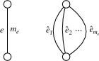
Figure 4: Edge duplication for an edge $e\in E$, i.e., duplicating the edge to the parallel edges of size $m_{e}$. With this manipulation, $m_{\hat{e}_{k}}$ becomes one for all duplicated edges $\hat{e}_{k}\in\hat{E}(e)$.

Let $\delta_{t}=\min_{k\in[t]}P^{k}(\bm{d}^{k-1})-P^{t-1}(\bm{d}^{t-1})$ be the optimality gap. The following lemma justificates the stopping criterion for algorithm 2.

Lemma 3.

Let $P^{T}_{\mathrm{LP}}$ be an optimal solution of (8) over $J_{T}=\{j_{1},j_{2},\dots,j_{T}\}$. If $\eta\geq\frac{2}{\varepsilon}\mathop{\rm depth}(G)\ln\frac{1}{\nu}$, then $\delta^{T+1}\leq\varepsilon/2$ implies $g-P^{T}_{\mathrm{LP}}\leq\varepsilon$, where $g$ is the guarantee of the base learner.

Note that if the algorithm always finds a hypothesis that maximizes the right-hand-side of (13), then this lemma guarantees the $\varepsilon$-accuracy to the optimal solution of (8).

Proof.

Let $P^{T}(\bm{d})$ be the objective function of (12) over $J_{T}=\{j_{1},j_{2},\dots,j_{T}\}$ obtained by algorithm 2 and let $\bm{d}^{T}$ be the optimal feasible solution of it. By the choice of $\eta$ and lemma 2, we get

$$\frac{1}{\eta}\sum_{e\in E}\left[d_{e}\ln\frac{d_{e}}{d^{0}_{e}}-d_{e}+d^{0}_{e}\right]\leq\frac{1}{\eta}\mathop{\rm depth}(G)\ln\frac{1}{\nu}\leq\frac{\varepsilon}{2}.$$

Thus, $P^{T}(\bm{d}^{T})\leq P^{T}_{\mathrm{L}P}+\varepsilon/2$. On the other hand, by the assumption on the weak learner, for any feasible solution $\bm{d}^{t-1}$, we obtain a $j_{t}\in[n+1]$ such that

$$g\leq\mathrm{sign}(j_{t})\sum_{e\in E}\mathrm{sign}(e)d^{t-1}_{e}.$$

Using the nonnegativity of the unnormalized relative entropy, we get

$$g\leq\min_{t\in[T+1]}\mathrm{sign}(j_{t})\sum_{e\in E}\mathrm{sign}(e)d^{t-1}_{e}\leq\min_{t\in[T+1]}P^{t}(\bm{d}^{t-1}).$$

Subtracting $P^{T}(\bm{d}^{T})$ from both sides, we get

$$g-P^{T}(\bm{d}^{T})\leq\min_{t\in[T+1]}P^{t}(\bm{d}^{t-1})-P^{t}(\bm{d}^{t})=\delta^{T+1}\leq\frac{\varepsilon}{2}.$$

Thus, $\delta_{T+1}\leq\varepsilon/2$ implies $g-P^{T}_{LP}\leq\varepsilon$. ∎

With lemma 3, We can obtain a similar iteration bound like ERLPBoost. To see that, we need to derive the dual problem of  (12). By standard calculation, you can verify that the dual problem becomes:

$$\max_{\bm{w},\bm{s},\bm{\beta}}\; \frac{1}{\eta}\sum_{e\in E}d^{0}_{e}\left(1-e^{-\eta A^{t}_{e}(\bm{w},\bm{s},\bm{\beta})}\right)+s_{\mathrm{root}}-s_{\mathrm{leaf}}-\frac{1}{\nu m}\sum_{e\in E}m_{e}\beta_{e}$$ (16)

sub. to. $$\sum_{j\in J_{t}}w_{j}=1,\bm{w}\geq\bm{0},\bm{\beta}\geq\bm{0}$$

$$A^{t}_{e}(\bm{w},\bm{s},\bm{\beta}):=\mathrm{sign}(e)\sum_{j\in J_{t}}\mathrm{sign}(j)I_{[j\in\Phi(e)]}w_{j}+s_{e.u}-s_{e.v}+\beta_{e},\quad\forall e\in E$$

Let $P^{t}(\bm{d})$, $D^{t}(\bm{w},\bm{s},\bm{\beta})$ be the objective function of the optimization sub-problems (12), (16), respectively. Let $\bm{d}^{t}$ be the optimal solution of (12) at round $t$ and similarly, let $(\bm{w}^{t},\bm{s}^{t},\bm{\beta}^{t})$ be the one of (16). Then, by KKT conditions, the following hold.

$$\sum_{j\in J_{t}}\mathrm{sign}(j)w^{t}_{j}\left[\sum_{e\in E:j\in\Phi(e)}\mathrm{sign}(e)d_{e}\right]=\max_{j\in J_{t}}\mathrm{sign}(j)\sum_{e\in E:j\in\Phi(e)}\mathrm{sign}(e)d_{e}$$ (17)

We will prove the following lemma, which corresponds to Lemma 2 in Warmuth et al. (2008).

Lemma 4.

If $\eta\geq 1/3$, then

$$P^{t}(\bm{d}^{t})-P^{t-1}(\bm{d}^{t-1})\geq\frac{1}{18\eta\mathop{\rm depth}(G)}\left[P^{t}(\bm{d}^{t-1})-P^{t-1}(\bm{d}^{t-1})\right]^{2},$$

where $\mathop{\rm depth}(G)$ denotes the max depth of graph $G$.

Proof.

First of all, we examine the right hand side of the inequality. By definition, $P^{t}(\bm{d}^{t-1})\geq P^{t-1}(\bm{d}^{t-1})$ and

$$P^{t}(\bm{d}^{t-1})-P^{t-1}(\bm{d}^{t-1})= \mathrm{sign}(j_{t})\sum_{e\in E:j_{t}\in\Phi(e)}\mathrm{sign}(e)d^{t-1}_{e}-\max_{j\in J_{t-1}}\mathrm{sign}(j)\sum_{e\in E:j\in\Phi(e)}\mathrm{sign}(e)d^{t-1}_{e}$$

$$= \mathrm{sign}(j_{t})\sum_{e\in E:j_{t}\in\Phi(e)}\mathrm{sign}(e)d^{t-1}_{e}-\sum_{j\in J_{t-1}}\mathrm{sign}(j)w^{t-1}_{j}\sum_{e\in E:j\in\Phi(e)}\mathrm{sign}(e)d^{t-1}_{e}$$

$$= \sum_{e\in E}\mathrm{sign}(e)d^{t-1}_{e}\left[\mathrm{sign}(j_{t})I_{[j_{t}\in\Phi(e)]}-\sum_{j\in J_{t-1}}\mathrm{sign}(j)I_{[j\in\Phi(e)]}w^{t-1}_{j}\right]$$

$$=: \sum_{e\in E}d^{t-1}_{e}x^{t}_{e},$$

where the second equality holds from (17).

Now, we will bound $P^{t}(\bm{d}^{t})-P^{t-1}(\bm{d}^{t-1})$ from below. For $\alpha\in[0,1]$, let

$$\bm{w}^{t}(\alpha):=(1-\alpha)\begin{bmatrix}\bm{w}^{t-1}\\ 0\end{bmatrix}+\alpha\begin{bmatrix}\bm{0}\\ 1\end{bmatrix}.$$ (18)

Since $(\bm{w}^{t},\bm{s}^{t},\bm{\beta}^{t})$ is the optimal solution of (12) at round $t$, $D^{t}(\bm{w}^{t},\bm{s}^{t},\bm{\beta}^{t})\geq D^{t}(\bm{w}^{t}(\alpha),\bm{s}^{t-1},\bm{\beta}^{t-1})$ holds. By strong duality,

$$P^{t}(\bm{d}^{t})-P^{t-1}(\bm{d}^{t-1})= D^{t}(\bm{w}^{t},\bm{s}^{t},\bm{\beta}^{t})-D^{t-1}(\bm{w}^{t-1},\bm{s}^{t-1},\bm{\beta}^{t-1})$$

$$\geq D^{t}(\bm{w}^{t}(\alpha),\bm{s}^{t-1},\bm{\beta}^{t-1})-D^{t-1}(\bm{w}^{t-1},\bm{s}^{t-1},\bm{\beta}^{t-1})$$

$$= \frac{1}{\eta}\sum_{e\in E}d^{0}_{e}\left(1-e^{-\eta A^{t}_{e}(\bm{w}^{t}(\alpha),\bm{s}^{t-1},\bm{\beta}^{t-1})}\right)-\frac{1}{\eta}\sum_{e\in E}d^{0}_{e}\left(1-e^{-\eta A^{t-1}_{e}(\bm{w}^{t-1},\bm{s}^{t-1},\bm{\beta}^{t-1})}\right)$$

$$= -\frac{1}{\eta}\sum_{e\in E}d^{0}_{e}\left(e^{-\eta A^{t}_{e}(\bm{w}^{t}(\alpha),\bm{s}^{t-1},\bm{\beta}^{t-1})}-e^{-\eta A^{t-1}_{e}(\bm{w}^{t-1},\bm{s}^{t-1},\bm{\beta}^{t-1})}\right).$$

By KKT conditions, we can write $\bm{d}^{t-1}$ in terms of the dual variables $(\bm{w}^{t-1},\bm{s}^{t-1},\bm{\beta}^{t-1})$:

$$d^{t-1}_{e}=d^{0}_{e}\exp\left[-\eta\left(\mathrm{sign}(e)\sum_{j\in J_{t-1}}\mathrm{sign}(j)I_{[j\in\Phi(e)]}w^{t-1}_{j}+s^{t-1}_{u}-s^{t-1}_{v}+\beta^{t-1}_{e}\right)\right]=d^{0}_{e}e^{-\eta A^{t-1}_{e}(\bm{w}^{t-1},\bm{s}^{t-1},\bm{\beta}^{t-1})}$$

Therefore,

$$P^{t}(\bm{d}^{t})-P^{t-1}(\bm{d}^{t-1})\geq-\frac{1}{\eta}\sum_{e\in E}d^{0}_{e}e^{-\eta A^{t-1}_{e}(\bm{w}^{t-1},\bm{s}^{t-1},\bm{\beta}^{t-1})}\left(e^{-\eta\alpha x^{t}_{e}}-1\right)=-\frac{1}{\eta}\sum_{e\in E}d^{t-1}_{e}\left(e^{-\eta\alpha x^{t}_{e}}-1\right).$$

Since $x^{t}_{e}\in[-2,+2]$, $\frac{3\pm x^{t}_{e}}{6}\in[0,1]$ and $\frac{3+x^{t}_{e}}{6}+\frac{3-x^{t}_{e}}{6}=1$. Thus, using Jensen’s inequality, we get

$$P^{t}(\bm{d}^{t})-P^{t-1}(\bm{d}^{t-1})\geq -\frac{1}{\eta}\sum_{e\in E}d^{t-1}_{e}\left(\exp\left[\frac{3+x^{t}_{e}}{6}(-3\eta\alpha)+\frac{3-x^{t}_{e}}{6}(3\eta\alpha)\right]-1\right)$$

$$\geq -\frac{1}{\eta}\sum_{e\in E}d^{t-1}_{e}\left(\frac{3+x^{t}_{e}}{6}e^{-3\eta\alpha}+\frac{3-x^{t}_{e}}{6}e^{3\eta\alpha}-1\right)=:R(\alpha).$$

The above inequality holds for all $\alpha\in[0,1]$. Here, $R(\alpha)$ is a concave function w.r.t. $\alpha$ so that we can choose the optimal $\alpha\in[0,1]$. By standard calculation, we get that the optimal $\alpha\in\mathbb{R}$ is

$$\alpha=\frac{1}{6\eta}\ln\frac{\sum_{e\in E}d^{t-1}_{e}(3+x^{t}_{e})}{\sum_{e\in E}d^{t-1}_{e}(3-x^{t}_{e})}$$ (19)

Since $x^{t}_{e}\leq 2$ for all $e\in E$, $\alpha\leq\frac{1}{6\eta}\ln\frac{\ln}{5}<\frac{1}{3\eta}$. Thus, $\alpha\leq 1$ holds. On the other hand, $\sum_{e\in E}d^{t-1}_{e}x^{t}_{e}\geq 0$ so that $\alpha\geq\frac{1}{6\eta}\ln 1=0$. Therefore, we can use (19) to lower-bound $P^{t}(\bm{d}^{t})-P^{t-1}(\bm{d}^{t-1})$.

$$P^{t}(\bm{d}^{t})-P^{t-1}(\bm{d}^{t-1})\geq -\frac{1}{\eta}\left[\frac{1}{3}\sqrt{\left(\sum_{e\in E}d^{t-1}_{e}(3+x^{t}_{e})\right)\left(\sum_{e\in E}d^{t-1}_{e}(3-x^{t}_{e})\right)}-\sum_{e\in E}d^{t-1}_{e}\right]$$

$$= -\frac{1}{\eta}\left[\frac{1}{3}\sqrt{9\left(\sum_{e\in E}d^{t-1}_{e}\right)^{2}-\left(\sum_{e\in E}d^{t-1}_{e}x^{t}_{e}\right)^{2}}-\sum_{e\in E}d^{t-1}_{e}\right]$$

By using the inequality

$$\forall a,b\geq 0,3a\geq b\implies\frac{1}{3}\sqrt{9a^{2}-b^{2}}-a\leq-\frac{b^{2}}{18a},$$

we get

$$P^{t}(\bm{d}^{t})-P^{t-1}(\bm{d}^{t-1})\geq \frac{1}{18\eta}\frac{\left(\sum_{e\in E}d^{t-1}_{e}x^{t}_{e}\right)^{2}}{\sum_{e\in E}d^{t-1}_{e}}$$

$$\geq \frac{1}{18\eta}\frac{\left(\sum_{e\in E}d^{t-1}_{e}x^{t}_{e}\right)^{2}}{\mathop{\rm depth}(G)}=\frac{1}{18\eta\mathop{\rm depth}(G)}\left[P^{t}(\bm{d}^{t-1})-P^{t-1}(\bm{d}^{t-1})\right]^{2},$$

which is the inequality we desire. ∎

We introduce the following lemma to prove the iteration bound of the compressed ERLPBoost.

Lemma 5 (Abe et al. (2001)).

Let $(\delta^{t})_{t\in\mathbb{N}}\subset\mathbb{R}_{\geq 0}$ be a sequence such that

$$\exists c>0,\forall t\geq 1,\delta^{t}-\delta^{t+1}\geq\frac{(\delta^{t})^{2}}{c}.$$

Then, the following inequality holds for all $t\geq 1$.

$$\delta^{t}\leq\frac{c}{t-1+\frac{c}{\delta^{1}}}$$

Proof of Theorem 4.

By definition of $\eta$, $\eta\geq 1/3$ holds. Thus, by lemma 4, we get

$$P^{t}(\bm{d}^{t})-P^{t-1}(\bm{d}^{t-1})\geq \frac{1}{18\eta\mathop{\rm depth}(G)}\left[P^{t}(\bm{d}^{t-1})-P^{t-1}(\bm{d}^{t-1})\right]^{2}$$

$$\geq \frac{1}{18\eta\mathop{\rm depth}(G)}\left[\min_{1\leq q\leq t}P^{q}(\bm{d}^{q-1})-P^{t-1}(\bm{d}^{t-1})\right]^{2}=\frac{(\delta^{t})^{2}}{18\eta\mathop{\rm depth}(G)}.$$

On the other hand,

$$P^{t}(\bm{d}^{t})-P^{t-1}(\bm{d}^{t-1})= \left(\min_{1\leq q\leq t}P^{q}(\bm{d}^{q-1})-P^{t-1}(\bm{d}^{t-1})\right)-\left(\min_{1\leq q\leq t}P^{q}(\bm{d}^{q-1})-P^{t}(\bm{d}^{t})\right)$$

$$\leq \left(\min_{1\leq q\leq t-1}P^{q}(\bm{d}^{q-1})-P^{t-1}(\bm{d}^{t-1})\right)-\left(\min_{1\leq q\leq t}P^{q}(\bm{d}^{q-1})-P^{t}(\bm{d}^{t})\right)$$

$$= \delta^{t-1}-\delta^{t}.$$

Thus, we get the following relation:

$$\delta^{t-1}-\delta^{t}\geq\frac{(\delta^{t})^{2}}{c\eta},\quad\text{where}\quad c=18\mathop{\rm depth}(G).$$

Lemma 5 gives us $\delta^{t}\leq\frac{c\eta}{t-1+\frac{c\eta}{\delta^{1}}}$. Rearranging this inequality, we get $T\leq\frac{c\eta}{\delta^{T}}-\frac{c\eta}{\delta^{1}}+1$. Since $\delta^{1}=\sum_{e\in E:j_{1}\in\Phi(e)}\mathrm{sign}(e)d^{0}_{e}\leq\mathop{\rm depth}(G)$, we have $\frac{c\eta}{\delta^{1}}\geq\frac{72}{\varepsilon}\mathop{\rm depth}(G)>1$. Therefore, the above inequality implies that $T\leq\frac{c\eta}{\delta^{T}}$. As long as the stopping criterion does not satisfy, $\delta^{t}>\varepsilon/2$ hold. Thus,

$$T\leq \frac{1}{\delta^{T}}\cdot 36\mathop{\rm depth}(G)\frac{2}{\varepsilon}\mathop{\rm depth}(G)\cdot\max\left(1,\ln\frac{1}{\nu}\right)$$

$$\leq \frac{144}{\varepsilon^{2}}\mathop{\rm depth}(G)^{2}\max\left(1,\ln\frac{1}{\nu}\right).$$

∎

7 Construction of NZDDs

We propose heuristics for constructing NZDDs given a subset family $S\subseteq 2^{\Sigma}$. We use the zcomp Toda (2013, 2015), developed by Toda, to compress the subset family $S$ to a ZDD. The zcomp is designed based on multikey quicksort Bentley and Sedgewick (1997) for sorting strings. The running time of the zcomp is $O(N\log^{2}|S|)$, where $N$ is an upper bound of the nodes of the output ZDD and $|S|$ is the sum of cardinalities of sets in $S$. Since $N\leq|S|$, the running time is almost linear in the input.

A naive application of the zcomp is, however, not very successful in our experiences. We observe that the zcomp often produces concise ZDDs compared to inputs. But, concise ZDDs do not always imply concise representations of linear constraints. More precisely, the output ZDDs of the zcomp often contains (i) nodes with one incoming edge or (ii) nodes with one outgoing edge. A node $v$ of these types introduces a corresponding variable $s_{v}$ and linear inequalities. Specifically, in the case of type (ii), we have $s_{v}\leq\sum_{j\Phi(e)}z^{\prime}_{j}+s_{e.u}$ for each $e\in E$ s.t. $e.v=v$, and for its child node $v^{\prime}$ and edge $e^{\prime}$ between $v$ and $v^{\prime}$, $s_{v^{\prime}}\leq\sum_{j\in\Phi(e^{\prime})}z^{\prime}_{j}+s_{v}$. These inequalities are redundant since we can obtain equivalent inequalities by concatenating them: $s_{v^{\prime}}\leq\sum_{j\in\Phi(e^{\prime})}z^{\prime}_{j}+\sum_{j\in\Phi(e)}z^{\prime}_{j}+s_{e.u}$ for each $e\in E$ s.t. $e.v=v$, where $s_{v}$ is removed.

Based on the observation above, we propose a simple reduction heuristics removing nodes of type (i) and (ii). More precisely, given an NZDD $G=(V,E)$, the heuristics outputs an NZDD $G^{\prime}=(V^{\prime},E^{\prime})$ such that $L(G)=L(G^{\prime})$ and $G^{\prime}$ does not contain nodes of type (i) or (ii). The heuristics can be implemented in O($|V^{\prime}|+|E^{\prime}|+\sum_{e\in E^{\prime}}|\Phi(e)|$) time by going through nodes of the input NZDD $G$ in the topological order from the leaf to the root and in the reverse order, respectively. The details of the heuristics is given in Appendix.

8 Experiments

We show preliminary experimental results on synthetic and real large data sets . We performed mixed integer programming and $1$-norm regularized soft margin optimization. Our experiments are conducted on a server with 2.60 GHz Intel Xeon Gold 6124 CPUs and 314GB memory. We use Gurobi optimizer 9.01, a state-of-the-art commercial LP solver. To obtain NZDD representations of data sets, we apply the procedure described in the previous section. The details of preprocessing of data sets and NZDD representations are shown in Appendix.

8.1 Mixed Integer programming on synthetic datasets

First, we apply our extended formulation (1) to mixed integer programming tasks over synthetic data sets. The problems are defined as the linear optimization with $n$ variables and $m$ linear constraints of the form $\bm{A}\bm{x}\geq\bm{b}$, where (i) each row of $\bm{A}$ has $k$ entries of $1$ and others are $0$s and nonzero entries are chosen randomly without repetition (ii) coefficients $a_{i}$ of linear objective $\sum_{i=1}^{n}{a_{i}x_{i}}$ is chosen from 1,…,100 randomly, and (iii) first $l$ variables take binary values in $\{0,1\}$ and others take real values in $[0,1]$. In our experiments, we fix $n=25,k=10$, $l=12$ and $m\in\{4\times 10^{5},8\times 10^{5}...,20\times 10^{5}\}$. We apply the Gurobi optimizer directly to the problem denoted as mip and the solver with pre-processing the problem by our extended formulation (denoted as nzdd_mip, respectively. The results are summarized in Figure 5. Our method consistently improves computation time for these datasets. This makes sense since it can be shown that when $m=O(n^{k})$ there exists an NZDD of size $O(nk)$ representing the constraint matrix. In addition, the pre-processing time is within 2 seconds in all cases.

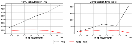
Figure 5: The comparison for synthetic datasets of a MIP problem. The horizontal axis represents the number of constraints of the original problem.

8.2 $1$-norm soft margin optimization on real data sets

Next, we apply our methods on the task of the $1$-norm soft margin optimization. This problem is a standard optimization problem in the machine learning literature, categorized as LP, for finding sparse linear classifiers given labeled instances. We compare the following methods using a naive LP solver.

1. a naive LP solver (denoted as naive),

2. LPBoost (Demiriz et al. (2002), denoted as lpb), a column generation-based method,

3. ERLPBoost (Warmuth et al. (2008), denoted as erlp), a modification of LPBoost with a non-trivial iteration bound.

4. a naive LP solver (denoted as nzdd_naive),

5. Algorithm 1 (denoted as nzdd_lpb),

6. Algorithm 2 (denoted as nzdd_erlpb).

Methods 1–3 solves the original soft margin optimization problem (4), while 4–6 solves the problem (6). We measure its computation time (CPU time) and maximum memory consumption, respectively, and compare their averages over parameters. Further, we performed $5$-fold cross validation to check the test error rates of our methods on real data sets. Table 2 shows that our formulation (6) is competitive with the original soft margin optimization.

We compare methods on some real data sets in the libsvm datasets Chang and Lin (2011) to see the effectiveness of our approach in practice. Generally, the datasets contain huge samples ($m$ varies from $3\times 10^{4}$ to $10^{7}$) with a relatively small size of features ($n$ varies from $20$ to $10^{5}$). The features of instances of each dataset is transformed into binary values. Note that these results exclude NZDD construction times since the compression takes around $1$ second, except for the HIGGS dataset (around $13$ seconds). Furthermore, the construction time of NZDDs can be neglected in the following reason: We often need to try multiple choices of the hyperparameters ($\nu$ in our case) and solve the optimization problem for each set of choices. But once we construct an NZDD, we can be re-use it for different values of hyperparameters without reconstructing NZDDs.

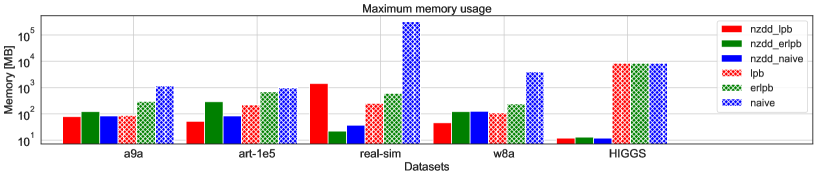
Figure 6: Comparison of maximum memory consumption of the soft margin optimization for real datasets. The y-axes are plotted in the logarithmic scale.

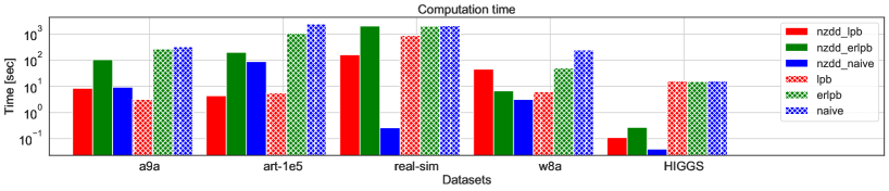
Figure 7: Comparison of running time of the soft margin optimization for real datasets. The y-axes are plotted in the logarithmic scale.

Table 2: Test error rates for real datasets

Data sets	lpb	nzdd_naive	nzdd_erlp
a9a	$0.174$	$0.159$	$0.157$
art-100000	$0.000$	$0.0004$	$0.004$
real-sim	$0.179$	$0.169$	$0.532$
w8a	$0.030$	$0.030$	$0.029$

$1$-norm soft margin optimization on synthetic datasets

We show experimental results for the $1$-norm soft margin optimization on synthetic datasets. We use a class of synthetic datasets that have small NZDD representations when the samples are large. First, we choose $m$ instances in $\{0,1\}^{n}$ uniformly randomly without repetition. Then we consider the following linear threshold function $f(\bm{x})=\mathrm{sign}(\sum_{j=1}^{k}x_{j}-r+1/2)$, where $k$ and $r$ are positive integers such that $1\leq r\leq k\leq n$). That is, $f(x)=1$ if and only if at least $r$ of the first $k$ components are $1$. Each label of the instance $\bm{x}\in\{0,1\}^{n}$ is labeled by $f(\bm{x})$. It can be easily shown that the whole labeled $2^{n}$ instances of $f$ is represented by an NZDD (or ZDD) of size $O(kr)$, which is exponentially small w.r.t. the sample size $m=2^{n}$. We fix $n=20$, $k=10$ and $r=5$. Then we use $m\in\{1\times 10^{5},2\times 10^{5}...,10^{6}\}$.

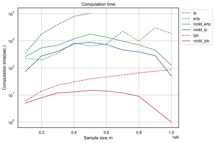
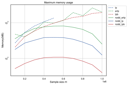
Figure 8: Comparison of computation times for synthetic datasets of the soft margin optimization. The y-axis is shown in the logarithmic scale. Results for naive w.r.t. $m\geq 6\times 10^{5}$ are omitted since it takes more than $1$ day $\approx 9\times 10^{4}$ seconds.

The results are given in Figure 8. As expected, our methods are significantly faster than comparators. Generally, our methods perform better than the standard counterparts. In particular, nzdd_lpb improves efficiency at least $10$ to $100$ times over others. Similar results are obtained for maximum memory consumption.

9 Conclusion

We proposed a generic algorithm of constructing an NZDD-based extended formulation for any given set of linear constraints with integer constraints as well as specific algorithms for the $1$-norm soft margin optimization and practical heuristics for constructing NZDDs. Our algorithms improve time/space efficiency on artificial and real datasets, especially when the datasets have concise NZDD representations.

10 Acknowledgements

We thank Mohammad Amin Mansouri for valuable discussions and initial development. This work was supported by JSPS KAKENHI Grant Numbers JP19H014174, JP19H04067,
JP20H05967, and JP22H03649, respectively.

Appendix A Details of heuristics for constructing NZDDs

A pseudo-code of the heuristics is given in Algorithm 3. Algorithm 3 consists of two phases. In the first phase, it traverses nodes in the topological order (from the leaf to the root), and for each node $v$ with one incoming edge $e$, it contracts $v$ with its parent node $u$ and $u$ inherits the edges $e^{\prime}$ from $v$. Label sets $\Phi(e)$ and $\Phi(e^{\prime})$ are also merged. The first phase can be implemented in $O(|V|+|E|)$ time, by using an adjacency list maintaining children of each node and lists of label sets for each edge. In the second phase, it does a similar procedure to simplify nodes with single outgoing edges. To perform the second phase efficiently, we need to re-organize lists of label sets before the second phase starts. This is because the lists of label sets could form DAGS after the first phase ends, which makes performing the second phase inefficient. Then, the second phase can be implemented in $O(|V^{\prime}|+|E^{\prime}|+\sum_{e\in E^{\prime}}|\Phi(e)|)$ time.

Algorithm 3 Reducing procedure

Input: NZDD $G=(V,E,\Phi,\Sigma)$

1. For each $u\in V$ in a topological order (from leaf to root) and for each child node $v$ of $u$,

   1. If indegree of $v$ is one,

      1. for the incoming edge $e$ from $u$ to $v$, each child node $v^{\prime}$ of $v$ and each outgoing edge $e^{\prime}$ from $v$ to $v^{\prime}$, add a new edge $e^{\prime\prime}$ from node $u$ to $v^{\prime}$ and set $\Phi(e^{\prime\prime})=\Phi(e)\cup\Phi(e^{\prime})$.

   2. Remove the incoming edge $e$ and all outgoing edges $e^{\prime}$.

2. For each $v\in V$ in a topological order (from root to leaf) and for each parent node $u$ of $v$,

   1. If outdegree of $u$ is one,

      1. for the outgoing edge $e$ of $u$, each parent node $u^{\prime}$ of $u$ and each outgoing edge $e^{\prime}$ from $u^{\prime}$ to $u$, add a new edge $e^{\prime\prime}$ from node $u^{\prime}$ to $v$ and set $\Phi(e^{\prime\prime})=\Phi(e)\cup\Phi(e^{\prime})$.

   2. Remove the outgoing edge $e$ and all incoming edges $e^{\prime}$.

3. Remove all nodes with no incoming and outgoing edges from $V$ and output the resulting DAG $G^{\prime}=(V^{\prime},E^{\prime})$.

Appendix B Details of experiments

Preprocessing of datasets

The datasets for the $1$-norm regularized soft margin optimization are obtained from the libsvm datasets. Some of them contain real-valued features. We convert them to binary ones by rounding them using $0.5$ as a threshold.

NZDD construction time and summary of datasets

Computation times for constructing NZDDs for the MIP synthetic datasets and synthetic and real datasets of the $1$norm regularized soft margin optimization are summarized in Table 3, 5 and 6, respectively. Note that the NZDD construction time is not costly and negligible in general because once we construct NZDDs, we can re-use those NZDDs for solving optimization problems with different objective functions or hyperparameters such as $\nu$ in the soft margin optimization.

Table 3: Computation time (seconds) of NZDD construction for synthetic MIP datasets, described in Table 4. All datasets have $n=25$ features and each instance have $k=10$ nonzero components.

$m$	zcomp	reducing procedure	Total
$4\times 10^{5}$	$0.39$	$1.02$	$1.41$
$8\times 10^{5}$	$0.76$	$1.38$	$2.14$
$12\times 10^{5}$	$1.08$	$1.41$	$2.49$
$16\times 10^{5}$	$1.36$	$1.10$	$2.46$
$20\times 10^{5}$	$1.60$	$0.33$	$1.93$

Table 4: Summary of synthetic datasets for MIP. The term “original” and “extended” mean the original and the extended formulations, respectively.

Data size		NZDD size		Variables		Constraints
$n$	$m$	$|V|$	$|E|$	Original	Extended	Original	Extended
$25$	$4\times 10^{5}$	$13,321$	$177,356$	$25$	$13,344$	$400,000$	$177,356$
$25$	$8\times 10^{5}$	$17,771$	$241,488$	$25$	$17,794$	$800,000$	$241,488$
$25$	$12\times 10^{5}$	$19,348$	$249,749$	$25$	$19,371$	$1,200,000$	$249,749$
$25$	$16\times 10^{5}$	$17,819$	$204,723$	$25$	$17,842$	$1,600,000$	$204,723$
$25$	$20\times 10^{5}$	$6,161$	$55,555$	$25$	$6,184$	$2,000,000$	$55,555$

Table 5: Computation times (seconds) for NZDD construction for the synthetic datasets, described in Table 7. all data have $n=20$ features.

$m$	zcomp	Reducing procedure	Total
$1\times 10^{5}$	$0.08$	$0.14$	$0.22$
$2\times 10^{5}$	$0.15$	$0.14$	$0.29$
$3\times 10^{5}$	$0.25$	$0.12$	$0.37$
$4\times 10^{5}$	$0.31$	$0.08$	$0.39$
$5\times 10^{5}$	$0.39$	$0.05$	$0.44$
$6\times 10^{5}$	$0.46$	$0.05$	$0.51$
$7\times 10^{5}$	$0.53$	$0.03$	$0.56$
$8\times 10^{5}$	$0.60$	$0.02$	$0.62$
$9\times 10^{5}$	$0.68$	$0.01$	$0.69$
$10\times 10^{5}$	$0.72$	$0.00$	$0.72$

Table 6: Computation times (seconds) for constructing NZDDs for real datasets of the soft margin optimization.

dataset	zcomp	Reducing procedure	Total
a9a	$0.04$	$0.20$	$0.24$
art-100000	$0.10$	$0.43$	$0.53$
real-sim	$0.24$	$0.99$	$1.23$
w8a	$0.27$	$4.20$	$4.47$
HIGGS	$13.13$	$0.00$	$13.13$

Table 8 summarizes the size of each problem for soft margin optimization. As this table shows, the extended formulations (6) have fewer variables and constraints. This is not surprising since the extended formulation has $O(n+|V|+|E|)$ variables and $O(|E|)$ constraints, while the original formulation (4) has $O(n+m)$ variables and $O(m)$ constraints.

Table 7: Summary of synthetic datasets for the soft margin optimization. The term “original” and “extended” mean the original and the extended formulations, respectively.

Data size		NZDD size		Variables		Constraints
$n$	$m$	$|V|$	$|E|$	Original	Extended	Original	Extended
$20$	$1\times 10^{5}$	$4,202$	$55,147$	$100,021$	$59,370$	$200,001$	$110,297$
$20$	$2\times 10^{5}$	$6,663$	$82,810$	$200,021$	$89,494$	$400,001$	$165,623$
$20$	$3\times 10^{5}$	$11,022$	$103,323$	$300,021$	$114,366$	$600,001$	$206,649$
$20$	$4\times 10^{5}$	$13,596$	$120,994$	$400,021$	$134,611$	$800,001$	$241,991$
$20$	$5\times 10^{5}$	$12,565$	$128,670$	$500,021$	$141,256$	$1,000,001$	$257,343$
$20$	$6\times 10^{5}$	$13,796$	$127,139$	$600,021$	$140,956$	$1,200,001$	$254,281$
$20$	$7\times 10^{5}$	$13,513$	$114,471$	$700,021$	$128,005$	$1,400,001$	$228,945$
$20$	$8\times 10^{5}$	$9,569$	$95,454$	$800,021$	$105,044$	$1,600,001$	$190,911$
$20$	$9\times 10^{5}$	$6,725$	$75,318$	$900,021$	$82,064$	$1,800,001$	$150,639$
$20$	$10\times 10^{5}$	$3,914$	$40,226$	$1,000,021$	$44,161$	$2,000,001$	$80,455$

Table 8: Summary of sizes of the real datasets of the soft margin optimization. The term “original” and “extended” mean the original and the extended formulations (4) and (6), respectively.

dataset	Data size		NZDD size		Variables		Constraints
	$n$	$m$	$|V|$	$|E|$	Original	Extended	Original	Extended
a9a	$123$	$32,561$	$775$	$20,657$	$32,685$	$21,556$	$65,123$	$41,317$
art-100000	$20$	$100,000$	$4,202$	$55,163$	$100,021$	$59,386$	$200,001$	$110,329$
real-sim	$20,955$	$72,309$	$38$	$7,922$	$93,265$	$28,916$	$144,619$	$15,847$
w8a	$300$	$49,749$	$209$	$34,066$	$50,050$	$34,576$	$99,499$	$68,135$
HIGGS	$28$	$11,000,000$	$151$	$989$	$11,000,029$	$1,169$	$22,000,001$	$1,981$

References

- Abe et al. [2001] N. Abe, J. Takeuchi, and M. K. Warmuth. Polynomial learnability of stochastic rules with respect to the KL-divergence and quadratic distance. IEICE Transactions on Information and Systems, E84-D(3):299–316, 2001.
- Bentley and Sedgewick [1997] J. L. Bentley and R. Sedgewick. Fast algorithms for sorting and searching strings. In Proceedings of the eighth annual ACM-SIAM symposium on Discrete algorithms (SODA’97), pages 360–369, 1997.
- Bergman et al. [2011] D. Bergman, W. J. van Hoeve, and J. N. Hooker. Manipulating MDD Relaxations for Combinatorial Optimization. In Proceedings of the 8th International Conference on Integration of AI and OR Techniques in Constraint Programming for Combinatorial Optimization Problems(CPAIOR 2011), volume 6697 of LNCS, pages 20–35, 2011.
- Bergman et al. [2016] D. Bergman, A. A. Cire, W.-J. van Hoeve, and J. Hooker. Decision Diagrams for Optimization. Springer Cham, 2016.
- Bryant [1986] R. E. Bryant. Graph-Based Algorithms for Boolean Function Manipulation. IEEE Transactions on Computers, C-35(8):677–691, aug 1986.
- Castro et al. [2019] M. P. Castro, A. A. Cire, and J. C. Beck. An MDD-Based Lagrangian Approach to the Multicommodity Pickup-and-Delivery TSP. INFORMS Journal on Computing, 32(2):263–278, sep 2019. ISSN 15265528. doi:10.1287/IJOC.2018.0881.
- Chang and Lin [2011] C.-C. Chang and C.-J. Lin. LIBSVM:a library for support vector machines. ACM Transactions on Intelligent Systems and Technology, 2(27):1–27, 2011.
- Conforti et al. [2010] M. Conforti, G. Cornuéjols, and G. Zambelli. Extended formulations in combinatorial optimization. 4OR, 8(1):1–48, 2010.
- Demiriz et al. [2002] A. Demiriz, K. P. Bennett, and J. Shawe-Taylor. Linear Programming Boosting via Column Generation. Machine Learning, 46(1-3):225–254, 2002.
- Duchi et al. [2011] J. Duchi, E. Hazan, and Y. Singer. Adaptive subgradient methods for online learning and stochastic optimization. Journal of machine learning research, 12(7):2121–2159, 2011.
- Fiorini et al. [2021] S. Fiorini, T. Huynh, and S. Weltge. Strengthening convex relaxations of 0/1-sets using Boolean formulas. Mathematical Programming, 190(1):467–482, 2021. ISSN 1436-4646. doi:10.1007/s10107-020-01542-w. URL https://doi.org/10.1007/s10107-020-01542-w.
- Freund and Schapire [1997] Y. Freund and R. E. Schapire. A Decision-Theoretic Generalization of On-Line Learning and an Application to Boosting. Journal of Computer and System Sciences, 55(1):119–139, 1997.
- Fujita et al. [2020] T. Fujita, K. Hatano, and E. Takimoto. Boosting over non-deterministic ZDDs. Theoretical Computer Science, 806:81–89, 2020.
- Goto et al. [2013] K. Goto, H. Bannai, S. Inenaga, and M. Takeda. Fast q-gram mining on SLP compressed strings. Journal of Discrete Algorithms, 18:89–99, 2013.
- Hermelin et al. [2009] D. Hermelin, G. M. Landau, S. Landau, and O. Weimann. A Unified Algorithm for Accelerating Edit-Distance Computation via Text-Compression. In Proceedings of the 26th International Symposium on Theoretical Aspects of Computer Science (STACS’09), volume LIPIcs, pages 529–540, 2009.
- Inoue et al. [2014] T. Inoue, K. Takano, T. Watanabe, J. Kawahara, R. Yoshinaka, A. Kishimoto, K. Tsuda, S.-i. Minato, and Y. Hayashi. Distribution Loss Minimization With Guaranteed Error Bound. IEEE Transactions on Smart Grid, 5(1):102–111, 2014.
- Jiang and Ravikumar [1993] T. Jiang and B. Ravikumar. Minimal NFA Problems are Hard. SIAM Journal on Computing, 22(6):1117–1141, 1993.
- Knuth [2011] D. E. Knuth. The Art of Computer Programming, Volume 4A, Combinatorial Algorithms,Part 1. Addison-Wesley Professional, 2011.
- Lifshits [2007] Y. Lifshits. Processing Compressed Texts: A Tractability Border. In Proceedings of the18th Annual Symposium on Combinatorial Pattern Matching (CPM’07), volume 4580 of LNCS, pages 228–240, 2007.
- Lohrey [2012] M. Lohrey. Algorithmics on SLP-compressed strings: A survey. Groups - Complexity - Cryptology, 4(2):241–299, 2012.
- Minato [1993] S.-i. Minato. Zero-Suppressed BDDs for Set Manipulation in Combinatorial Problems. In Proceedings of the 30th international Design Automation Conference (DAC’93), pages 272–277, 1993.
- Minato [2017] S.-i. Minato. Power of Enumeration — Recent Topics on BDD/ZDD-Based Techniques for Discrete Structure Manipulation. IEICE Transactions on Information and Systems, E100.D(8):1556–1562, 2017.
- Minato and Uno [2010] S.-i. Minato and T. Uno. Frequentness-Transition Queries for Distinctive Pattern Mining from Time-Segmented Databases. In Proceedings of the 2010 SIAM International Conference on Data Mining (SDM), pages 339–349, 2010.
- Minato et al. [2008] S.-i. Minato, T. Uno, and H. Arimura. LCM over ZBDDs: Fast Generation of Very Large-Scale Frequent Itemsets Using a Compact Graph-Based Representation. In Proceedings of the 12th Pacific-Asia Conference onKnowledge Discovery and Data Mining (PAKDD’08), volume 5012 of LNAI, pages 234–246, 2008.
- Morrison et al. [2016] D. R. Morrison, E. C. Sewell, and S. H. Jacobson. Solving the Pricing Problem in a Branch-and-Price Algorithm for Graph Coloring Using Zero-Suppressed Binary Decision Diagrams. INFORMS Journal on Computing, 28(1):67–82, jan 2016. ISSN 15265528. doi:10.1287/IJOC.2015.0667.
- Nishino et al. [2014] M. Nishino, N. Yasuda, S.-i. Minato, and M. Nagata. Accelerating Graph Adjacency Matrix Multiplications with Adjacency Forest. In Proceedings of the 2014 SIAM International Conference on Data Mining (SDM 14), pages 1073–1081, 2014.
- Raina et al. [2009] R. Raina, A. Madhavan, and A. Y. Ng. Large-scale deep unsupervised learning using graphics processors. In Proceedings of the 26th annual international conference on machine learning (ICML’09), pages 873–880, 2009.
- Rätsch and Warmuth [2005] G. Rätsch and M. K. Warmuth. Efficient Margin Maximizing with Boosting. Journal of Machine Learning Research, 6:2131–2152, 2005.
- Rytter [2004] W. Rytter. Grammar Compression, LZ-Encodings, and String Algorithms with Implicit Input. In Proceedings of the 31st International Colloquium of Automata, Languages and Programming (ICALP’04), volume 3142 of LNCS, pages 15–27, Berlin, Heidelberg, 2004.
- Tabei et al. [2016] Y. Tabei, H. Saigo, Y. Yamanishi, and S. J. Puglisi. Scalable Partial Least Squares Regression on Grammar-Compressed Data Matrices. In Proceedings of the 22nd ACM SIGKDD International Conference on Knowledge Discovery and Data Mining (KDD ’16), pages 1875–1884, 2016.
- Toda [2013] T. Toda. Fast Compression of Large-Scale Hypergraphs for Solving Combinatorial Problems. In Proceedings of 16th International Conference on Discovery Science (DS’13), volume 8140 of LNAI, pages 281–293, Berlin, Heidelberg, 2013. Springer Berlin Heidelberg. ISBN 978-3-642-40897-7.
- Toda [2015] T. Toda. ZCOMP: Fast Compression of Hypergraphs into ZDDs, 2015. URL http://www.sd.is.uec.ac.jp/toda/code/zcomp.html.
- Warmuth et al. [2007] M. Warmuth, K. Glocer, and G. Rätsch. Boosting Algorithms for Maximizing the Soft Margin. In Advances in Neural Information Processing Systems 20 (NIPS 2007), pages 1585–1592, 2007.
- Warmuth et al. [2008] M. Warmuth, K. Glocer, and S. V. N. Vishwanathan. Entropy Regularized LPBoost. In Proceedings of the 19th International Conference on Algorithmic Learning Theory (ALT’08), pages 256–271, 2008.
- Yannakakis [1991] M. Yannakakis. Expressing combinatorial optimization problems by Linear Programs. Journal of Computer and System Sciences, 43(3):441–466, 1991. ISSN 0022-0000. doi:https://doi.org/10.1016/0022-0000(91)90024-Y.