Coherent Equalization of Linear Quantum Systems

Abstract

This paper introduces the $H_{\infty}$-like methodology of coherent filtering for equalization of passive linear quantum systems to help mitigate degrading effects of quantum communication channels. For such systems, we seek to find a suboptimal equalizing filter which is itself a passive quantum system. The problem amounts to solving an optimization problem subject to constraints dictated by the requirement for the equalizer to be physically realizable. By formulating these constraints in the frequency domain, we show that the problem admits a convex $H_{\infty}$-like formulation. This allows us to derive a set of suboptimal coherent equalizers using $J$-spectral factorization. An additional semidefinite relaxation combined with the Nevanlinna-Pick interpolation is shown to lead to a tractable algorithm for the design of a suboptimal coherent equalizer.

and

1 Introduction

The main aim of this paper is to demonstrate an application of the optimization paradigm to the derivation of coherent filters for quantum systems, i.e., filters which themselves can be realized as a quantum system. Such filters are highly desirable in quantum engineering since they do not require conventional non-quantum measurement devices and hence are able to deliver technological advantages of quantum information processing. To be concrete, we focus on one type of the optimal coherent filtering problem concerned with equalization of distortions of quantum signals transmitted via a quantum communication channel to help mitigate degrading effects of the channel. Owing to the analogy with classical channel equalization, we call this problem the quantum equalization problem.

Optimization has proven to be an essential tool in the design of classical communication and signal processing systems. The Wiener filtering theory [29] is the best known demonstration of how degrading effects of noise and the channel can be mitigated using optimization techniques. While the Wiener’s solution is elegant and tractable in the case of stationary signals and perfectly known channels, additional properties and requirements on the signal, the channel or the filter impose further optimization constraints [2, 30]. This is precisely the situation encountered in the derivation of a coherent quantum filter, as such filter must satisfy the fundamental constraints of physical realizability, in order to represent a valid quantum physical system; see [13, 22, 20, 16] and references therein.

[width=0.7]bsplusbs

Figure 1: A quantum optical communication system consisting of two beam splitters acting as a channel and a filter, respectively.

Conditions for physical realizability of quantum control systems have received considerable attention in the control literature, in the context of coherent quantum control and estimation problems including problems of coherent $H_{\infty}$ control [13, 17], coherent quantum LQG control [19] and coherent filtering [27]. These conditions ensure that the controller/filter can be implemented as a quantum physical device. Fig. 1 illustrates this situation. The quantum optical beam splitter on the left represents a network of static quantum optical devices acting as a quantum communication channel. The channel transmits a message $\breve{u}$ which suffers from degradation due to the channel’s physical environment $\breve{w}$. The device on the right is another quantum physical device acting as a filter aiming to reduce this degradation while being subjected to its own degrading environment $\breve{z}$. The general aim of the coherent equalization problem is to design quantum systems able to recover the transmitted message with high fidelity and which are realizable as physical quantum devices. In this paper we develop a procedure for the synthesis of transfer functions for such equalizing filters.

Our focus is on the question whether distortions introduced by a passive quantum communication channel can be efficiently mitigated using another passive quantum system acting as a filter. Even restricted to passive filters, this question is meaningful and sufficiently rich. Indeed, transfer functions corresponding to passive coherent filters are easily implementable by cascading quantum optical components such as beam splitters, optical cavities and phase shift devices [18, 20]. Therefore, answering the question as to whether a (sub)optimal coherent equalizer can be obtained within the class of passive systems enables synthesis of physical devices which solve coherent equalization problems. The paper gives examples of such synthesis.

The requirement for physical realizability makes the task of finding an optimal coherent filter quite nontrivial [27]. In [27], this requirement led to nonconvex constraints on the state-space matrices of the filter which prohibited obtaining a closed form solution. In this paper, following [26, 25], we cast the coherent equalization problem in the frequency domain. It turns out that in the frequency domain the physical realizability constraints have a convenient structure. They can be partitioned so that the constraints on the ‘key’ variables which determine the filter performance can be separated from the constraints on the ‘slack variables’ responsible for the physical realizability of the filter. This leads us to adopt a two-step procedure for the design of coherent suboptimal filters which was originally proposed in [26]. In the first step of this procedure, only some of the physical realizability constraints are retained, and the filter performance is optimized over the ‘key’ variables subject to these constraints. We call this problem the auxiliary optimization problem. In the second step, the remaining variables of the filter are computed to fulfill the requirement of physical realizability. The rigorous justification of this procedure is one of the original contributions of the paper.

In contrast with the previous work [27, 26, 25] concerned with developing coherent Wiener and Kalman filters, we consider the problem in the vein of classical $H_{\infty}$ filtering [9, 23]. Also unlike the coherent $H_{\infty}$ control problem [13, 17], our approach is concerned with minimization of the largest eigenvalue of the power spectrum density (PSD) matrix of the equalization error. This allowed us to formulate the aforementioned auxiliary optimization problem as a convex optimization problem whose constraints are frequency dependent. This approach led to two contributions. Firstly, we characterize the class of causal suboptimal coherent filters in a manner similar to the Youla parameterization of $H_{\infty}$ suboptimal controllers [35], via the technique of $J$-spectral factorization [8, 12]. Secondly, we propose a Semidefinite Program (SDP) relaxation which reduces the number of optimization constraints to a finite number of constraints. Combined with the method of Nevanlinna-Pick interpolation [1, 3, 15] this gives a tractable algorithm to obtain a physically realizable suboptimal filter.

The optimization approach allows us to reveal some peculiar features of coherent equalizers which set them apart from measurement-based filters. It turns out that, unlike the classical equalization problem, the mean-square error between the input and output fields of a linear quantum system may not always be improved using a coherent linear equalizer. This is consistent with the earlier finding [26] that in the simplest case when both the input field and the thermal noise field have one degree of freedom and the channel is static, the coherent equalization is truly beneficial when the signal-to-noise ratio is below a certain threshold. The paper relates the existence of such threshold to the question whether a certain frequency dependent Linear Matrix Inequality (LMI) is feasible, as a sufficient condition in the general case.

The paper is organized as follows. In the next section we present the background on physically realizable open linear quantum systems. The coherent equalization problem is also introduced in Section 2 where it is posed as an $H_{\infty}$-like filtering problem subject to the physical realizability constraints. The justification of the two-step procedure for the design of coherent suboptimal filters and the auxiliary optimization problem are presented in Section 3. The relation between the feasibility sets of this auxiliary problem and the corresponding classical problem is also discussed in Section 3. A complete characterization of all suboptimal solutions for the auxiliary optimization problem is derived in Section 4. An alternative suboptimal solution to this auxilialry problem via semidefinite programming and Nevanlinna-Pick interpolation is presented in Section 5. Section 6 presents two examples which illustrate these results. In the first example, the results are applied to a single mode system consisting of static components. The second example is an optical cavity system. For both examples, we show how a suboptimal equalizer can be constructed via $J$-spectral factorization, and also illustrate the semidefinite programming approach undertaken in Section 5. In the first example, we also show that the bound on the performance delivered via the $J$-spectral factorization approach is in fact tight, and that an optimal equalizer can be obtained as a limit point of the set of suboptimal equalizers derived using the $J$-spectral factorization. This example also illustrates the threshold on the signal-to-noise ratio of the input fields that arises due to the requirement of physical realizability. Conclusions and suggestions for future work are given in Section 7.

Notation

For a collection of operators $\mathbf{a}_{1}$, …, $\mathbf{a}_{n}$ in a Hilbert space $\mathfrak{H}$, the notation $\mathrm{col}(\mathbf{a}_{1},\ldots,\mathbf{a}_{n})$ denotes the column vector of operators obtained by concatenating operators $\mathbf{a}_{j}$, i.e., the operator mapping $\mathfrak{H}$ into the cartesian product of $n$ copies of the space $\mathfrak{H}$, $\mathfrak{H}^{n}$. For an operator $\mathbf{a}:\mathfrak{H}\to\mathfrak{H}$, $\mathbf{a}^{*}$ denotes the adjoint operator, and when $\mathbf{a}=\mathrm{col}(\mathbf{a}_{1},\ldots,\mathbf{a}_{n})$, $\mathbf{a}^{\#}$ denotes the column vector of adjoint operators, $\mathbf{a}^{\#}=\mathrm{col}(\mathbf{a}_{1}^{*},\ldots,\mathbf{a}_{n}^{*})$, $\mathbf{a}^{T}=(\mathbf{a}_{1}~{}\ldots~{}\mathbf{a}_{n})$ (i.e, the row of operators), and $\mathbf{a}^{\dagger}=(\mathbf{a}^{\#})^{T}$. Also, we will use the notation $\breve{\mathbf{a}}=\mathrm{col}(\mathbf{a},\mathbf{a}^{\#})=\mathrm{col}(\mathbf{a}_{1},\ldots,\mathbf{a}_{n},\mathbf{a}_{1}^{*},\ldots,\mathbf{a}_{n}^{*})$. $[\mathbf{a},\mathbf{b}]$ denotes the commutator of the operators $\mathbf{a},\mathbf{b}$ in $\mathfrak{H}$, $[\mathbf{a},\mathbf{b}]=\mathbf{a}\mathbf{b}-\mathbf{b}\mathbf{a}$. The quantum expectation of an operator $\mathbf{v}$ of a quantum system in a state $\rho$ is denoted $\langle\mathbf{v}\rangle=\mathop{\rm tr}\nolimits[\rho\mathbf{v}]$ [21]. For a complex number $a$, $a^{*}$ is its complex conjugate and for a matrix $A=(A_{ij})$, $A^{\#}$, $A^{T}$, $A^{\dagger}$ denote, respectively, the matrix of complex conjugates $(A_{ij}^{*})$, the transpose matrix and the Hermitian adjoint matrix. $I$ is the identity matrix, and $J=\left[\begin{array}[]{rr}I&0\\ 0&-I\end{array}\right].$ We will also write $I_{n}$ when we need to specify that this is the $n\times n$ identity matrix. For two complex matrices $X_{-}$, $X_{+}$, we write $\Delta(X_{-},X_{+})=\left[\begin{array}[]{cc}X_{-}&X_{+}\\ X_{+}^{\#}&X_{-}^{\#}\end{array}\right].$ When $X_{-}=X_{-}(s)$, $X_{+}=X_{+}(s)$ are complex transfer function matrices, the stacking operation defines the transfer function matrix $\Delta(X_{-}(s),X_{+}(s))=\left[\begin{array}[]{cc}X_{-}(s)&X_{+}(s)\\ (X_{+}(s^{*}))^{\#}&(X_{-}(s^{*}))^{\#}\end{array}\right].$ For a transfer function matrix $X(s)$, $X(s)^{H}$ denotes its Hermitian para-conjugate, $X(s)^{H}=X(-s^{*})^{\dagger}$. Clearly, for a complex matrix $X$, $X^{H}=X^{\dagger}$. When the matrix $X$ is Hermitian, $\boldsymbol{\sigma}(X)$ is the largest eigenvalue of $X$. For a transfer function $X(s)$ in the Hardy space $H_{\infty}$ of matrix-valued functions which are analytic in the open right half-plane $\mathrm{Re}s>0$ and are bounded on the imaginary axis, $\|X\|_{\infty}$ denotes its $H_{\infty}$ norm, $\|X\|_{\infty}=\sup_{\mathrm{Re}s>0}\|X(s)\|=\mathrm{ess}\sup_{\omega\in\mathbf{R}}\|X(i\omega)\|$, where $\|\cdot\|$ is the induced 2-norm of a matrix [35].

2 Coherent equalization problem for linear quantum communication systems

2.1 Quantum noise processes

In the Heisenberg picture of quantum mechanics, an open quantum system can be modeled as a linear system describing evolution of $m$ harmonic modes driven by $n$ quantum input noise processes [11, 7, 34]. These quantum input processes are represented as annihilation and creation operators $\mathbf{b}(t)=\mathrm{col}(\mathbf{b}_{1}(t),\ldots,\mathbf{b}_{n}(t))$, $\mathbf{b}^{\#}(t)=\mathrm{col}(\mathbf{b}^{\#}_{1}(t),\ldots,\mathbf{b}^{\#}_{n}(t))$, acting in an appropriate Fock space [11] and satisfying canonical commutation relations $[\breve{\mathbf{b}}(t),\breve{\mathbf{b}}^{\dagger}(t^{\prime})]=J\delta(t-t^{\prime})$; here $\delta(t)$ is the delta function. However from the system theory viewpoint they can be treated as quantum random processes. When the input fields are in a Gaussian state with zero mean, which is the situation considered in this paper, these random processes can be regarded as stationary quantum Gaussian white noise processes with zero mean (i.e., $\langle\breve{\mathbf{b}}(t)\rangle=0$) and the correlation function

$$\langle\breve{\mathbf{b}}(t)\breve{\mathbf{b}}^{\dagger}(t^{\prime})\rangle=F_{\mathbf{b}}\delta(t-t^{\prime}),\quad F_{\mathbf{b}}\triangleq\left[\begin{array}[]{cc}I+\Sigma_{\mathbf{b}}^{T}&\Pi_{\mathbf{b}}\\ \Pi_{\mathbf{b}}^{\dagger}&\Sigma_{\mathbf{b}}\end{array}\right].$$ (3)

The matrix $F_{\mathbf{b}}$ symbolizes intensity of the process $\breve{\mathbf{b}}$; $\Sigma_{\mathbf{b}}$ is a nonnegative definite complex Hermitian matrix, $\Sigma_{\mathbf{b}}^{\dagger}=\Sigma_{\mathbf{b}}$, and $\Pi_{\mathbf{b}}$ is a complex symmetric matrix, $\Pi_{\mathbf{b}}^{T}=\Pi_{\mathbf{b}}$. In this paper, we will consider linear quantum systems in thermal state, therefore it will always be assumed that $\Pi_{\mathbf{b}}=0$.

2.2 A quantum communication system

We consider a general setup consisting of a linear quantum system representing a communication channel and a second linear quantum system acting as an equalizer, as shown in Fig. 2.

[width=0.7]general-e

Figure 2: A general quantum communication system. The transfer function $\Gamma(s)$ represents the channel, and $\Xi(s)$ represents an equalizing filter.

The $n$-dimensional input vector field $\breve{u}$ plays the role of a signal carrying a message transmitted through the channel, and the $n_{w}$-dimensional vector of operators $\breve{w}$ is comprised of operators describing the environment as well as noises introduced by the routing hardware such as beam splitters, etc. In what follows it is assumed that these operators commute, $[\breve{u},\breve{w}]=0,$ and the system is in a Gaussian thermal state, and $\langle\breve{u}(t)\rangle=0$, $\langle\breve{w}(t)\rangle=0$. Furthermore, it is assumed that the input fields $\breve{u}$ and $\breve{w}$ are not correlated, $\langle\breve{u}(t)\breve{w}^{\dagger}(t^{\prime})\rangle=0$.

To represent the communication channel as a linear quantum system, the annihilation and creation parts of $\breve{u}$, $\breve{w}$ are stacked together to form the vectors of operators $\mathbf{b}=\mathrm{col}(u,w)$ and $\mathbf{b}^{\#}=\mathrm{col}(u^{\#},w^{\#})$, which are then combined into the vector $\breve{\mathbf{b}}$. This combined vector of input operators $\breve{\mathbf{b}}$ is applied to a linear quantum system with the transfer function $\Gamma(s)$ which represents the communication channel . The annihilation and creation operators of the output field of this system form the vector $\breve{\mathbf{y}}=\mathrm{col}(y,d,y^{\#},d^{\#})$. The dimensions of the annihilation operators $y$ and $d$ (respectively, creation operators $y^{\#}$ and $d^{\#}$) of the output field are $n$ and $n_{w}$, respectively.

A coherent equalizer is another linear quantum system $\Xi(s)$ which takes the components $\breve{y}=\mathrm{col}(y,y^{\#})$ of the output $\breve{\mathbf{y}}$ as one of its inputs. Its second input $\breve{z}(t)=\mathrm{col}(z(t),z^{\#}(t))$ in Fig. 2 is comprised of $n_{z}$ annihilation and creation operators of the auxiliary noise input field introduced into the filter model to make it physically realizable [13, 28]. For simplicity, we assume that the filter environment is in a Gaussian vacuum state; that is, the filter’s quantum noise process $\breve{z}(t)$ has zero mean, $\langle\breve{z}(t)\rangle=0$, and the correlation function $\langle\breve{z}(t)\breve{z}^{\dagger}(t^{\prime})\rangle=\left[\begin{array}[]{cc}I_{n_{z}}&0\\ 0&0\end{array}\right]\delta(t-t^{\prime}),$ i.e., $\Sigma_{z}=0$, $\Pi_{z}=0$. The operator $\breve{z}$ commutes with $\breve{u}$ and $\breve{w}$.

The input into the equalizer, $\breve{\mathbf{b}}_{\textrm{eq}}=\mathrm{col}(\mathbf{b}_{\textrm{eq}},\mathbf{b}_{\textrm{eq}}^{\#})$, combines the output $\breve{y}$ of the channel and the filter environment noise $\breve{z}$, so that $\mathbf{b}_{\textrm{eq}}=\mathrm{col}(y,z)$. Its output is $\breve{\mathbf{y}}_{\textrm{eq}}=\mathrm{col}(\mathbf{y}_{\textrm{eq}},\mathbf{y}_{\textrm{eq}}^{\#})$, and each of the vectors of operators $\mathbf{y}_{\textrm{eq}},\mathbf{y}_{\textrm{eq}}^{\#}$ can be partitioned into operator vectors whose dimensions match the dimensions of $y$ and $z$, respectively: $\mathbf{y}_{\textrm{eq}}=\mathrm{col}(\hat{u},\hat{z})$, $\mathbf{y}_{\textrm{eq}}^{\#}=\mathrm{col}(\hat{u}^{\#},\hat{z}^{\#})$. We designate the first component of these partitions, namely $\hat{u}$ (respectively $\hat{u}^{\#}$), as the output field of the equalizing filter.

2.3 The coherent equalization problem

Let $e(t)$ be the difference between the channel input and the filter output fields, $e(t)=\hat{u}(t)-u(t)$. We refer to $e(t)$ as the equalization error of the filter $\Xi(s)$. Let $P_{e}(i\omega)$ denote the Fourier transform of the autocorrelation matrix $R_{e}(t)=\langle e(t)e(0)^{\dagger}\rangle$. $P_{e}(i\omega)$ represents the power spectrum density of the difference between the channel input and the filter output fields. The coherent equalization problem in this paper is to obtain a physically realizable passive filter transfer function $\Xi$ which minimizes (exactly or approximately) the largest eigenvalue of $P_{e}(i\omega)$:

$$\Xi=\mathrm{arg}\inf_{\Xi}\sup_{\omega}\boldsymbol{\sigma}(P_{e}(i\omega)).$$ (4)

A formal definition of the problem will be given in Section 2.6, after we present some necessary background on linear quantum systems and the notion of physical realizability.

2.4 Open quantum systems

This paper adopts linear quantum system models for quantum channels and equalizing filters [7, 20]. In the Heisenberg picture, dynamics of an open quantum linear system consisting of $m$ quantum oscillators interacting with the environment described by Gaussian input fields are represented using quantum stochastic differential equations [11] which describe evolution of annihilation and creation operators of the quantum system in the underlying Hilbert space $\mathfrak{H}$. The Heisenberg-Langevin form of these equations is as follows,

$$\dot{\breve{\mathbf{a}}}(t) = \breve{A}\breve{\mathbf{a}}(t)+\breve{B}\breve{\mathbf{b}}(t),$$

$$\breve{\mathbf{y}}(t) = \breve{C}\breve{\mathbf{a}}(t)dt+\breve{D}\breve{\mathbf{b}}(t).$$ (5)

Here, $\breve{\mathbf{b}}(t)$ denotes an $2n_{b}$-dimensional vector of quantum random processes defined in Section 2.1. The vector $\breve{\mathbf{a}}$ consists of the mode operators $\mathbf{a}=\mathrm{col}(\mathbf{a}_{1},\ldots\mathbf{a}_{m})$ and their adjoint operators $\mathbf{a}^{\#}=\mathrm{col}(\mathbf{a}_{1}^{*},\ldots\mathbf{a}_{m}^{*})$; at the initial time $t=t_{0}$ these operators represent initial annihilation and creation operators of the system $\mathbf{a}(t_{0})=\mathrm{col}(\mathbf{a}_{1}(t_{0}),\ldots,\mathbf{a}_{m}(t_{0}))$, $\mathbf{a}^{\#}(t_{0})=\mathrm{col}(\mathbf{a}_{1}^{*}(t_{0}),\ldots,\mathbf{a}_{m}^{*}(t_{0}))$, respectively. Without loss of generality, we assume throughout the paper that $[\mathbf{a}(t_{0}),\mathbf{a}^{\dagger}(t_{0})]=I$. Also, $\breve{\mathbf{y}}=\mathrm{col}(\mathbf{y},\mathbf{y}^{\#})$ denotes the output field of the system that carries away information about the system interacting with the input field $\breve{\mathbf{b}}$; the vectors of operators $\mathbf{y}=\mathscr{col}(\mathbf{y}_{1},\ldots,\mathbf{y}_{n_{b}})$, $\mathbf{y}^{\#}=\mathscr{col}(\mathbf{y}_{1}^{*},\ldots,\mathbf{y}_{n_{b}}^{*})$, have the same dimension $n_{b}$ as the dimension of the vectors $\mathbf{b}$, $\mathbf{b}^{\#}$ of the input field. The matrices $\breve{A}$, $\breve{B}$, $\breve{C}$, $\breve{D}$ are complex matrices partitioned in accordance with the structure of the vectors of operators $\breve{\mathbf{a}}$, $\breve{\mathbf{b}}$, as

$$\breve{A} = \Delta(A_{-},A_{+}),\quad\breve{B}=\Delta(B_{-},B_{+}),$$

$$\breve{C} = \Delta(C_{-},C_{+}),\quad\breve{D}=\Delta(D_{-},D_{+}).$$

A detailed discussion of open linear quantum systems can be found in [14, 7, 13, 34].

In the subsequent sections we will consider passive linear quantum systems. For such systems, $A_{+}=0$, $B_{+}=0$, $C_{+}=0$, $D_{+}=0$, i.e., the evolution of the ‘annihilation part’ of the system variable $\breve{\mathbf{a}}$ is governed only by the annihilation operators $\mathbf{b}(t)$ of the input field, and the ‘creation’ part of $\breve{\mathbf{a}}$ is driven by the creation operators $\mathbf{b}^{\#}(t)$ [14]. In this case, the matrices $\breve{A}$, $\breve{B}$, $\breve{C}$, $\breve{D}$ are block diagonal.

For a quantum stochastic differential equation of the form (2.4) to describe evolution of quantum physical system in the Heisenberg picture, its coefficients must satisfy certain additional conditions [22, 13, 16]. These conditions, known as the physical realizability conditions, ensure that the oscillator variables $\mathbf{a}_{j}(t)$ and the output field operators $\mathbf{y}_{j}(t)$ defined by equation (2.4) evolve unitarily,

$$\mathbf{a}_{j}(t)=\boldsymbol{\mathsf{U}}^{*}(t-t_{0})\mathbf{a}_{j}(t_{0})\boldsymbol{\mathsf{U}}(t-t_{0}),\quad j=1,\ldots m,$$

$$\mathbf{y}_{k}(t)=\boldsymbol{\mathsf{U}}^{*}(t-t_{0})\mathbf{y}_{k}(t_{0})\boldsymbol{\mathsf{U}}(t-t_{0}),\quad k=1,\ldots n.$$

Here $\boldsymbol{\mathsf{U}}(t)$ is an adapted process of unitary operators of the system. The physical realizability of the system amounts to the existence of such operators; more precisely the operator process $\boldsymbol{\mathsf{U}}(t)$ arises as a solution to a certain Ito quantum stochastic differential equation [11].

In the frequency domain, the input-output map defined by system (2.4) is expressed in terms of the $n_{b}\times n_{b}$ transfer function

$$\Gamma(s)=\breve{C}(sI_{2m}-\breve{A})^{-1}\breve{B}+\breve{D},$$

relating the bilateral Laplace transforms of $\breve{\mathbf{y}}(t)$ and $\breve{\mathbf{b}}(t)$  [7, 34]. According to the next lemma, physical realizability of the linear quantum system (2.4) dictates that the transfer function $\Gamma(s)$ must be $J$-symplectic; see [22, 7, 1]. The lemma is a straightforward combination of Theorem 4 in [22] and Theorem 6.1.1 in [1]. It requires the following assumption about the linear quantum system (2.4).

Assumption 1.

The pair $(\breve{A},\breve{B})$ is controllable, and the pair $(\breve{A},\breve{C})$ is observable.

Lemma 1.

Suppose Assumption 1 is satisfied. Then the following conditions are equivalent:

1. The linear quantum system (2.4) is physically realizable;

2. $\breve{D}=\Delta(S,0)$ where $S$ is a unitary matrix, and

   $$\Gamma(s)J\Gamma(s)^{H}=\Gamma(s)^{H}J\Gamma(s)=J;$$ (6)

3. $\breve{D}=\Delta(S,0)$ where $S$ is a unitary matrix, and

   $$\Gamma(i\omega)J\Gamma(i\omega)^{\dagger}=\Gamma(i\omega)^{\dagger}J\Gamma(i\omega)=J.$$ (7)

When the system (2.4) is a passive (annihilation only) system, its transfer function $\Gamma(s)$ is block-diagonal [7]

$$\Gamma(s)=\left[\begin{array}[]{cc}G(s)&0\\ 0&G(s^{*})^{\#}\end{array}\right],$$ (10)

where $G(s)$ is the transfer function of the annihilation part of the system, $G(s)=C_{-}(sI-A_{-})^{-1}B_{-}+S$. Assumption 1 reduces to the assumption that $(A_{-},B_{-})$ and $(A_{-},C_{-})$ are controllable and observable, respectively. It then follows from this assumption that the matrices $A_{-}$ and $\breve{A}=\Delta(A_{-},0)$ are Hurwitz and that $G(s)$ and $\Gamma(s)$ in (10) are stable rational proper transfer functions. Furthermore, the frequency domain physical realizability relations (6), (7) reduce to the condition that $G(s)$ is paraunitary and $G(i\omega)$ is unitary (also see [16]),

$$G(s)^{H}G(s)=G(s)G(s)^{H}=I,$$ (11)

$$G(i\omega)^{\dagger}G(i\omega)=G(i\omega)G(i\omega)^{\dagger}=I.$$ (12)

Then $G(i\omega)$ is bounded at infinity and analytic on the entire closed imaginary axis [32, Lemma 2].

Introduce the partition of the transfer function $G(s)$ compatible with the partition $\mathbf{b}=\mathrm{col}(u,w)$, $\mathbf{y}=\mathrm{col}(y,d)$,

$$G(s) = \left[\begin{array}[]{cc}G_{11}(s)&G_{12}(s)\\ G_{21}(s)&G_{22}(s)\\ \end{array}\right].$$ (15)

Using this partition, the physical realizability condition (11) reduces to the identities

$$G_{11}(s)G_{11}(s)^{H}+G_{12}(s)G_{12}(s)^{H}=I,$$ (16a)

$$G_{11}(s)G_{21}(s)^{H}+G_{12}(s)G_{22}(s)^{H}=0,$$ (16b)

$$G_{21}(s)G_{21}(s)^{H}+G_{22}(s)G_{22}(s)^{H}=I.$$ (16c)

We conclude this section by presenting a frequency domain relationship between power spectrum densities of the input and the stationary output fields of the linear quantum system (2.4). Since we focus on passive systems, we restrict attention to the autocorrelation matrix of $\mathbf{y}$, $R_{\mathbf{y}}(t)=\langle\mathbf{y}(t)\mathbf{y}^{\dagger}(0)\rangle$. The corresponding power spectrum density (PSD) matrix $P_{\mathbf{y}}(s)$ is the bilateral Laplace transform of $R_{\mathbf{y}}(t)$ [34]. It was shown in [34] that since the matrix $\breve{A}$ is Hurwitz, it holds that

$$P_{\mathbf{y}}(i\omega)=G(i\omega)(I+\Sigma_{\mathbf{b}}^{T})G(i\omega)^{\dagger}.$$ (17)

2.5 Physically realizable passive filters

Since the focus of this paper is on passive coherent filters, from now only the filters of the form $\Xi(s)=\Delta(H(s),0)$ will be considered, where $H(s)$ is an $(n+n_{z})\times(n+n_{z})$ transfer function. According to Lemma 1, physical realizability of the filter requires that $H(s)$ must be a paraunitary transfer function matrix and the matrix $H(i\omega)$ must be unitary; cf. (11), (12):

$$H(s)H(s)^{H}=I,\quad H(i\omega)H(i\omega)^{\dagger}=I.$$ (18)

The set of equalizers $\Xi(s)=\Delta(H(s),0)$, where $H(s)$ satisfies (18) will be denoted $\mathscr{H}_{p}$.

The transfer function matrix $H(s)$ can be further partitioned into the blocks compatible with dimensions of the filter inputs $\mathrm{col}(y,z)$ and outputs $\mathrm{col}(\hat{u},\hat{z})$:

$$H(s)=\left[\begin{array}[]{cc}H_{11}(s)&H_{12}(s)\\ H_{21}(s)&H_{22}(s)\end{array}\right].\qquad$$ (21)

Using this partition, the condition (18) can be expanded into conditions of the form (16) which provide an explicit set of constraints imposed on the transfer functions of each of the filter channels by the requirement for physical realizability

$$H_{11}(s)H_{11}(s)^{H}+H_{12}(s)H_{12}(s)^{H}=I,$$ (22a)

$$H_{11}(s)H_{21}(s)^{H}+H_{12}(s)H_{22}(s)^{H}=0,$$ (22b)

$$H_{21}(s)H_{21}(s)^{H}+H_{22}(s)H_{22}(s)^{H}=I.$$ (22c)

2.6 The formal problem statement

Let $e(t)=\hat{u}(t)-u(t)$ be the equalization error introduced in Section 2.3. We then write that $\breve{e}(t)=\mathrm{col}(e(t),e^{\#}(t))$. The transfer function from the combined ‘input plus channel and filter environment’ field $\breve{\mathbf{v}}=\mathrm{col}(u,w,z,u^{\#},w^{\#},z^{\#})$ to $\breve{e}$ is obtained by interconnecting the passive channel and passive filter systems as shown in Fig. 2,

$$E(s) = \Delta(E_{-}(s),0),$$

$$E_{-}(s) \triangleq \left[\begin{array}[]{c|c|c}H_{11}(s)G_{11}(s)-I{}&~{}H_{11}(s)G_{12}(s){}&~{}H_{12}(s)\end{array}\right].\qquad$$ (24)

Using this transfer function and (17), the Fourier transform of the autocorrelation matrix of the equalization error $R_{e}(t)=\langle e(t)e(0)^{\dagger}\rangle$ can be expressed as

$$P_{e}(i\omega) = \left[\begin{array}[]{cc}E_{-}(i\omega)&0\end{array}\right]F_{\mathbf{v}}\left[\begin{array}[]{c}E_{-}(i\omega)^{\dagger}\\ 0\end{array}\right].$$ (28)

Here $F_{\mathbf{v}}$ is the intensity matrix of the noise process $\breve{\mathbf{v}}$ when the system is in a thermal quantum state (cf. (3)),

$$F_{\mathbf{v}} = \left[\begin{array}[]{ccc|ccc}I+\Sigma_{u}^{T}&0&0&0&0&0\\ 0&I+\Sigma_{w}^{T}&0&0&0&0\\ 0&0&~{}I{}&0&0&0\\ \hline\cr 0&0&0&\Sigma_{u}&0&0\\ 0&0&0&0&~{}\Sigma_{w}{}&0\\ 0&0&0&0&0&0\end{array}\right].$$ (35)

Since $F_{\mathbf{v}}^{\dagger}=F_{\mathbf{v}}$, $P_{e}(i\omega)$ is an $n\times n$ Hermitian matrix where $n$ is the dimension of the ‘channel input’ $u$. Hence the eigenvalues of $P_{e}(i\omega)$ are real.

Using (24) and (35) an explicit expression for $P_{e}(i\omega)$ can be obtained [26],

$$P_{e}(i\omega)$$ (36)

$$= (H_{11}(i\omega)G_{11}(i\omega)-I)(I+\Sigma_{u}^{T})(G_{11}(i\omega)^{\dagger}H_{11}(i\omega)^{\dagger}-I)$$

$$+ H_{11}(i\omega)G_{12}(i\omega)(I+\Sigma_{w}^{T})G_{12}(i\omega)^{\dagger}H_{11}(i\omega)^{\dagger}$$

$$+ H_{12}(i\omega)H_{12}(i\omega)^{\dagger}.$$

Taking advantage of the properties (16a) and (22a) due to passivity of the channel and filter transfer functions, this expression can be simplified:

$$P_{e}(i\omega)=H_{11}(i\omega)\Psi(i\omega)H_{11}(i\omega)^{\dagger}$$ (37)

$$- H_{11}(i\omega)G_{11}(i\omega)(I+\Sigma_{u}^{T})-(I+\Sigma_{u}^{T})G_{11}(i\omega)^{\dagger}H_{11}(i\omega)^{\dagger}$$

$$+ \Sigma_{u}^{T}+2I$$

where we let

$$\Psi(s)\triangleq G_{11}(s)\Sigma_{u}^{T}G_{11}(s)^{H}+G_{12}(s)\Sigma_{w}^{T}G_{12}(s)^{H}.$$ (38)

In the sequel, we will also make use of the $n\times n$ matrix

$$P_{e}(s)=\left[\begin{array}[]{cc}E_{-}(s)&0\end{array}\right]F_{\mathbf{v}}\left[\begin{array}[]{c}E_{-}(s)^{H}\\ 0\end{array}\right]$$

$$= H_{11}(s)\Psi(s)H_{11}(s)^{H}-H_{11}(s)G_{11}(s)(I+\Sigma_{u}^{T})$$

$$- (I+\Sigma_{u}^{T})G_{11}(s)^{H}H_{11}(s)^{H}+\Sigma_{u}^{T}+2I.$$ (43)

Again, this expression is obtained using the identities (16a) and (22a). We will also write $P_{e}(s,H)$ when we need to stress that the expression for $P_{e}(s)$ corresponds to a specific filter $\Xi(s)=\Delta(H(s),0)$.

We now present a formal statement of the problem of coherent passive equalization posed in Section 2.3.

Problem 1.

The guaranteed cost passive equalization problem is to obtain a transfer function matrix $\Xi(s)=\Delta(H(s),0)\in\mathscr{H}_{p}$ which ensures a desired bound on the power spectrum density of the equalization error. That is, given $\gamma>0$, obtain $\Xi(s)=\Delta(H(s),0)\in\mathscr{H}_{p}$ such that

$$P_{e}(i\omega)<\gamma^{2}I_{n}\quad\forall\omega.$$ (44)

The optimal passive equalization problem is to minimize the bound (44) in the class of filters $\mathscr{H}_{p}$:

$$\gamma_{\circ}\triangleq\inf\gamma\mbox{ subject to $\gamma>0$ and (\ref{eq:6'.sub})}.$$ (45)

In Problem 1 we tacitly replaced optimization of $\sup_{\omega}\boldsymbol{\sigma}(P_{e}(i\omega))$ with (45). The two problems are equivalent. Indeed, given $\gamma>0$, define the set

$$\mathscr{H}_{\gamma}=\{H(s)\colon\sup_{\omega}\boldsymbol{\sigma}(P_{e}(i\omega,H))<\gamma^{2},H(s)H(s)^{H}=I\}.$$

Lemma 2.

$$\gamma_{\circ}=\bar{\gamma}\triangleq\inf\{\gamma>0\colon\mathscr{H}_{\gamma}\neq\emptyset\}.$$ (46)

Proof: From the definition of $\bar{\gamma}$, there exists a sequence $\{\gamma_{k}\}\subset\{\gamma>0\colon\mathscr{H}_{\gamma}\neq\emptyset\}$ such that $\gamma_{k}\geq\bar{\gamma}$ and $\lim_{k\to\infty}\gamma_{k}=\bar{\gamma}$. That is, for any $\epsilon>0$, one can choose a sufficiently large $k$ so that $\gamma_{k}<\bar{\gamma}+\epsilon$. Also, since $\mathscr{H}_{\gamma_{k}}\neq\emptyset$, there exists a passive $H_{k}(s)$ such that $\sup_{\omega}\boldsymbol{\sigma}(P_{e}(i\omega,H_{k}))<\gamma_{k}^{2}$. Consequently, $P_{e}(i\omega,H_{k})<\gamma_{k}^{2}I_{n}$ for any $\omega$, therefore $\gamma_{\circ}\leq\gamma_{k}<\bar{\gamma}+\epsilon$. Letting $\epsilon\to 0$ implies that $\gamma_{\circ}\leq\bar{\gamma}$.

Conversely, according to the definition of $\gamma_{\circ}$, there exists a sequence of constants $\{\gamma_{l}^{\prime}\}$, $\gamma_{l}^{\prime}\geq\gamma_{\circ}$, which converges to $\gamma_{\circ}$ and such that for each $\gamma_{l}^{\prime}$ there exists a physically realizable $H_{l}(s)$ such that $P_{e}(i\omega,H_{l})<(\gamma_{l}^{\prime})^{2}I_{n}$ for any $\omega$. Then $\sup_{\omega}\boldsymbol{\sigma}(P_{e}(i\omega,H_{l}))\leq(\gamma_{l}^{\prime})^{2}<(\gamma_{l}^{\prime}+\epsilon)^{2}$, where $\epsilon>0$ is an arbitrarily small constant. Thus, $\mathscr{H}_{\gamma_{l}^{\prime}+\epsilon}\neq\emptyset$, which means that $\bar{\gamma}\leq\gamma_{l}^{\prime}+\epsilon$. Letting $l^{\prime}\to\infty$, $\epsilon\to 0$ leads to the conclusion that $\bar{\gamma}\leq\gamma_{\circ}$. Thus, $\bar{\gamma}=\gamma_{\circ}$. $\Box$

Lemma 2 indicates that Problem 1 is analogous to the classical $H_{\infty}$ filtering problem [9]. However, instead of the singular value of the disturbance-to-error transfer function, we seek to optimize the largest eigenvalue of the PSD function $P_{e}$. Importantly, Problem 1 belongs to the class of constrained optimization problems since the class of admissible filters is restricted to physically realizable passive filters.

3 The framework for solving Problem 1

3.1 The procedure for the synthesis of coherent equalizers

The expression for $P_{e}$ obtained in (37) depends only on $H_{11}$ and does not depend explicitly on other blocks of the matrix $H$. Therefore we adopt a two-step procedure to solve Problem 1 which was originally proposed in [26]. In the first step of this procedure, the power spectrum density of the equalization error will be optimized with respect to $H_{11}(s)$ subject to some of the constraints implied by the paraunitarity of $H$. Next, the blocks $H_{12}(s)$, $H_{21}(s)$, $H_{22}(s)$ of the equalizer transfer function will be computed to fulfill the constraint (22). However, [26] did not explain how causal $H_{12}(s)$, $H_{21}(s)$, $H_{22}(s)$ can be computed. This problem is solved in this section. For this, we recall the notion of spectral factors of a rational para-Hermitian transfer function matrix [32].

Lemma 3 (Youla, Theorem 2 of [32]).

Suppose a rational para-Hermitian $n\times n$ transfer function matrix $X(s)$ is positive semidefinite on the imaginary axis, $X(i\omega)\geq 0$, and has normal rank $r$, $r\leq n$. Then the following statements hold.

1. There exists an $r\times n$ rational matrix $N(s)$ such that $X(s)=N(s)^{H}N(s)$. $N(s)$ is a spectral factor of $X(s)$.

2. $N(s)$ and its right inverse $N^{-1}(s)$ are both analytic in the open right half-plane $\mathrm{Re}s>0$.

3. $N(s)$ is unique up to a constant unitary $r\times r$ matrix multiplier on the left; i.e., if $N_{1}(s)$ also satisfies (a) and (b), then $N_{1}(s)=TN(s)$ where $T$ is an $r\times r$ constant unitary matrix.

4. If $X(s)$ is analytic on the finite $i\omega$ axis, then $N(s)$ is analytic in a right half-plane $\mathrm{Re}s>-\tau$, $\exists\tau>0$. If in addition, the normal rank of $X(s)$ is invariant on the finite $i\omega$ axis, then $N^{-1}(s)$ is also analytic in a right half plane $\mathrm{Re}s>-\tau_{1}$, $\exists\tau_{1}>0$.

5. By applying claims (a)-(d) to $X(s)^{T}$, one can obtain the factorization $X(s)=M(s)M(s)^{H}$, where the spectral factor $M(s)$ has the dimension $n\times r$ and has the same analiticity properties as $N(s)$.

Consider a proper rational transfer function $H_{11}(s)$ with the properties

1. $H_{11}(s)$ has poles in the open left half-plane of the complex plane, and is analytic in a right half-plane $\mathrm{Re}s>-\tau$ ($\exists\tau>0$);

2. $H_{11}(i\omega)H_{11}(i\omega)^{\dagger}\leq I_{n}$; and

3. The normal rank of the following matrices does not change on the finite imaginary axis $i\omega$:

   $$X_{1}(s) = I_{n}-H_{11}(s)H_{11}(s)^{H},$$

   $$X_{2}(s) = I_{n}-H_{11}(s)^{H}H_{11}(s).$$ (47)

The transfer functions $X_{1}(s)$ and $X_{2}(s)$ defined in (3) are para-Hermitian, and according to (H1), $X_{1}(i\omega)$ and $X_{2}(i\omega)$ are positive semidefinite. Therefore, according to Lemma 3 these matrices admit spectral factorizations

$$X_{1}(s)=H_{12}(s)H_{12}(s)^{H},\quad X_{2}(s)=\tilde{H}_{21}(s)^{H}\tilde{H}_{21}(s).\quad$$ (48)

Also, let $\tilde{H}_{21}^{-1}(s)$ denote the right inverse of $\tilde{H}_{21}(s)$, $\tilde{H}_{21}(s)\tilde{H}_{21}^{-1}(s)=I_{r},$ where $r$ is the normal rank of $X_{2}(s)$.

Theorem 1.

Given a proper rational transfer function $H_{11}(s)$ which satisfies conditions (H1)–(H3), let $H_{12}(s)$ and $\tilde{H}_{21}(s)$ be the spectral factors from (48). Define

$$H_{21}(s)=U(s)\tilde{H}_{21}(s),$$

$$H_{22}(s)=-U(s)(\tilde{H}_{21}^{-1}(s))^{H}H_{11}(s)^{H}H_{12}(s),\quad$$ (49)

where $U(s)$ is a stable causal paraunitary $r\times r$ transfer function matrix, chosen to cancel unstable poles of $(\tilde{H}_{21}^{-1}(s))^{H}H_{11}(s)^{H}H_{12}(s)$; cf. [23]. The corresponding $(n+r)\times(n+r)$ transfer function $H(s)$ in (21) is stable, causal and satisfies (18).

Proof: For simplicity of notation, we drop the argument $s$ of the transfer functions.

Since $H_{11}$ is a proper rational stable transfer function, it is causal according to the Paley-Wiener Theorem [31]. Furthermore since $H_{11}$ is analytic in a right half-plane $\mathrm{Re}s>-\tau$ ($\exists\tau>0$), it is analytic on the imaginary axis. Together with the condition that the normal rank of $H_{11}$ does not change along the imaginary axis, this guarantees that the spectral factors $H_{12}$, $\tilde{H}_{21}$ and the right inverse $\tilde{H}_{21}^{-1}$ are analytic in a right half-plane $\mathrm{Re}s>-\tau$, $\exists\tau>0$; see claim (d) of Lemma 3. These properties ensure that the rational transfer functions $H_{12}$, $\tilde{H}_{21}$ and $\tilde{H}_{21}^{-1}$ are stable and causal; the latter conclusion follows from the Paley-Wiener Theorem. Stability and causality of $H_{21}$, $H_{22}$ now follow from their definitions expressed in terms of stable causal $H_{11}$, $H_{12}$, $\tilde{H}_{21}$ and $\tilde{H}_{21}^{-1}$.

We now show that $H$ is paraunitary. The identity (22a) follows directly from the first identity in (48). Also, using (48), the identity (22b) can be verified:

$$H_{11}H_{21}^{H}+H_{12}H_{22}^{H}$$ (50)

$$= (H_{11}\tilde{H}_{21}^{H}-H_{12}H_{12}^{H}H_{11}(s)\tilde{H}_{21}^{-1})U^{H}$$

$$= (H_{11}\tilde{H}_{21}^{H}-H_{11}(I-H_{11}^{H}H_{11})\tilde{H}_{21}^{-1})U^{H}$$

$$= (H_{11}\tilde{H}_{21}^{H}-H_{11}\tilde{H}_{21}^{H}\tilde{H}_{21}\tilde{H}_{21}^{-1})U^{H}=0.$$

Furthermore, (22c) also holds:

$$H_{21}H_{21}^{H}+H_{22}H_{22}^{H}$$ (51)

$$= U(\tilde{H}_{21}\tilde{H}_{21}^{H}+(\tilde{H}_{21}^{-1})^{H}H_{11}^{H}H_{12}H_{12}^{H}H_{11}\tilde{H}_{21}^{-1})U^{H}$$

$$= U(\tilde{H}_{21}\tilde{H}_{21}^{H}$$

$$+(\tilde{H}_{21}^{-1})^{H}(H_{11}^{H}H_{11}-H_{11}^{H}H_{11}H_{11}^{H}H_{11})\tilde{H}_{21}^{-1})U^{H}$$

$$= U(\tilde{H}_{21}\tilde{H}_{21}^{H}+(\tilde{H}_{21}^{-1})^{H}(I-\tilde{H}_{21}^{H}\tilde{H}_{21}$$

$$-(I-\tilde{H}_{21}^{H}\tilde{H}_{21})(I-\tilde{H}_{21}^{H}\tilde{H}_{21}))\tilde{H}_{21}^{-1})U^{H}$$

$$= UU^{H}=I.$$

$\Box$

Remark 1.

Theorem 1 shows that the number of noise channels $z$, $z^{\#}$ necessary to ensure that the equalizing filter is physically realizable is determined by the normal rank of $I_{n}-H_{11}(s)^{H}H_{11}(s)$. In particular, when $H_{11}(s)^{H}H_{11}(s)=I$, the transfer function $H_{11}(s)$ is physically realizable, and additional noise channels are not required. $\Box$

3.2 The auxiliary optimization problem

In the remainder of the paper, the two-step procedure described in the previous section will pave the way to developing optimization approaches to solving the quantum equalizer design problem. For a constant $\gamma>0$, define the feasible set $\mathscr{H}_{11,\gamma}$ consisting of proper rational $n\times n$ transfer function matrices $H_{11}(s)$, which satisfy conditions (H1), (H2) and (44). For convenience, we summarize the two latter conditions as

$$P_{e}(i\omega,H_{11})<\gamma^{2}I_{n},$$ (52)

$$H_{11}(i\omega)H_{11}(i\omega)^{\dagger}\leq I_{n}\quad\forall\omega\in\mathbf{R}.$$ (53)

In (52), we slightly abuse the notation and write $P_{e}(i\omega,H_{11})$ for the expression on the right hand side of (37), to emphasize that the independent variable of this function is $H_{11}(s)$. Note that feasible $H_{11}$ are elements of the Hardy space $H_{\infty}$ and  (53) implies $\|H_{11}\|_{\infty}\leq 1$.

Theorem 1 leads us to replace Problem 1 with the following auxiliary optimization problem.

Problem 1’.

The auxiliary guaranteed cost problem is to obtain, for a given $\gamma>0$, a feasible $H_{11}(s)\in\mathscr{H}_{11,\gamma}$. The corresponding auxiliary optimal filtering problem is to determine an optimal level of guaranteed performance

$$\gamma_{\circ}^{\prime}=\inf\{\gamma>0\colon\mathscr{H}_{11,\gamma}\neq\emptyset\}.$$ (54)

Formally, one must distinguish between $\gamma_{\circ}$ defined in (45) and $\gamma_{\circ}^{\prime}$ defined in Problem 1’. Solutions of the latter problem are not guaranteed to satisfy condition (H3) of Theorem 1, therefore $\gamma_{\circ}^{\prime}\leq\gamma_{\circ}$. Nevertheless, the remainder of the paper focuses on the auxiliary Problem 1’. We will observe later in Section 6 that the (sub)optimal transfer functions $H_{11}(s)\in\mathscr{H}_{11,\gamma}$ obtained in the examples considered in that section also satisfy (H3). Therefore, the gap between $\gamma_{\circ}^{\prime}$ and $\gamma_{\circ}$ vanishes in those examples.

Note that when $\gamma^{2}\geq\boldsymbol{\sigma}(\Sigma_{u}^{T}+2I)$ (equivalently, $\gamma^{2}I\geq\Sigma_{u}^{T}+2I$), the auxiliary guaranteed cost problem has a trivial solution since for such $\gamma$, the set $\mathscr{H}_{11,\gamma}$ contains $H_{11}(s)=0$. In this case, a trivial suboptimal filter in $\mathscr{H}_{\gamma}$ can be readily constructed using Theorem 1, e.g., $H(s)=\left[\begin{array}[]{cc}0&I\\ I&0\end{array}\right]$. Therefore, the standing assumption in the remainder of the paper is that

$$\gamma^{2}<\boldsymbol{\sigma}(\Sigma_{u}^{T}+2I).$$ (55)

3.3 Relation to the classical $H_{\infty}$-like equalization

The constraint (53) reflects the distinction between the coherent equalization problem and its classical $H_{\infty}$-like counterpart. The latter involves optimization of the bound on the PSD matrix $P_{e}$ but does not include condition (53):

$$\gamma_{*}=\inf\gamma,$$ (56)

$$\mbox{subject to }\gamma>0,\quad P_{e}(i\omega,H_{11})<\gamma^{2}I_{n}\quad\forall\omega\in\mathbf{R}.$$

Clearly, for every $\gamma>0$, the set $\mathscr{H}_{11,\gamma}$ of feasible optimizers $H_{11}$ of Problem 1’ is a subset of the feasible set of the problem (56). On the other hand, later in the paper we will encounter a situation in which a suboptimal filter of problem (56) also satisfies (53). Via the S-procedure, such situation can be related to feasibility of a semidefinite program.

Theorem 2.

Suppose $\gamma\geq\gamma_{*}$. If there exists $\theta>0$ such that $\forall\omega\in\mathbf{R}$

$$\theta\left[\begin{array}[]{cc}\Psi(i\omega)&-G_{11}(i\omega)(I_{n}+\Sigma_{u}^{T})\\ -(I_{n}+\Sigma_{u}^{T})G_{11}(i\omega)^{\dagger}&~{}~{}\Sigma_{u}^{T}+(2-\gamma^{2})I_{n}\end{array}\right]-J\geq 0,$$ (57)

then the feasible set of problem (56) is equal to the feasible set of Problem 1’ $\mathscr{H}_{11,\gamma}$.

Proof: After pre- and postmultyping (57) by $[H_{11}(i\omega)~{}I_{n}]$ and $\left[\begin{array}[]{c}H_{11}(i\omega)^{\dagger}\\ I_{n}\end{array}\right]$, respectively, (57) becomes

$$\theta(P_{e}(i\omega,H_{11})-\gamma^{2}I_{n})-(H_{11}(i\omega)H_{11}(i\omega)^{\dagger}-I_{n})\geq 0.$$

Now let $H_{11}(s)$ be a feasible transfer function of problem (56), such that $P_{e}(i\omega,H_{11})<\gamma^{2}I$ $\forall\omega$. Then

$$H_{11}(i\omega)H_{11}(i\omega)^{\dagger}\leq I_{n}+\theta(P_{e}(i\omega,H_{11})-\gamma^{2}I_{n})\leq I_{n}.$$

That is, $H_{11}(s)\in\mathscr{H}_{11,\gamma}$. This shows that under the conditions of the theorem, the feasible set of problem (56) is a subset of $\mathscr{H}_{11,\gamma}$. Thus, the claim of the theorem follows, due to the previous observation that the converse inclusion also holds. $\Box$

From Theorem 2, it follows that under condition (57), the constraint (53) of problem (54) is inactive and any suboptimal filter of problem (56) is also a guaranteed cost filter for Problem 1’.

4 Parameterization of suboptimal causal physically realizable filters

In this section, we will derive a parametric representation of the set $\mathscr{H}_{11,\gamma}$ of feasible optimizers of Problem 1’, given a $\gamma>\gamma_{\circ}^{\prime}$.

The problem of characterizing all causal rational proper transfer functions which satisfy (52), (53) is similar to the problem of describing suboptimal $H_{\infty}$ filters for a linear uncertain system, with the additional constraint that $\|H_{11}\|_{\infty}\leq 1$. We apply the technique of $J$-spectral factorization [8, 12] to solve this problem under the following technical assumption.

Assumption 2.

The matrix $\Psi(s)$ in (38) has full normal rank.

Next, we note that $\Psi(s)$ and its transpose $\Psi(s)^{T}$ are proper rational para-Hermitian matrices, $\Psi(s)^{H}=\Psi(s)$, $\Psi(-s^{*})^{\#}=\Psi(s)^{T}$. Therefore, according to Lemma 3, applied to $\Psi(s)^{T}$, there exists a rational matrix $M(s)$ such that

$$\Psi(s)=M(s)M(s)^{H}.$$ (58)

Under Assumption 2, the matrix $M$ is a square $n\times n$ matrix, and its left inverse $M^{-1}(s)$ is the same as its right inverse. Since the matrix $\breve{A}$ of the channel system is assumed to be stable (Assumption 1), $G_{11}(s)$, $G_{12}(s)$ are analytic on the imaginary axis. Therefore $\Psi(s)$ is also analytic on the imaginary axis and $\Psi(i\omega)\geq 0$ for all $\omega$. Then according to Lemma 3, $M(s)$ and $M^{-1}(s)$ are analytic in a right half-plane $\mathrm{Re}s>-\tau$, $\exists\tau>0$. These observations allow us to express the expression for $P_{e}(s,H_{11})-\gamma^{2}I$ as

$$P_{e}(s,H_{11})-\gamma^{2}I_{2n}=\left[\begin{array}[]{cc}Y(s)&I_{n}\end{array}\right]\Phi(s)\left[\begin{array}[]{c}Y(s)^{H}\\ I_{n}\end{array}\right],\quad$$ (62)

where $Y(s)=H_{11}(s)M(s)$, and

$$\Phi(s)=\left[\begin{array}[]{cc}I_{n}&Q(s)\\ Q(s)^{H}&~{}~{}\Sigma_{u}^{T}+(2-\gamma^{2})I_{n}\end{array}\right],$$ (65)

$$Q(s)\triangleq-M^{-1}(s)G_{11}(s)(I_{n}+\Sigma_{u}^{T}),$$ (66)

$Q(s)$ is analytic in a right half-plane $\mathrm{Re}s>-\tau$, $\exists\tau>0$.

Recall that $(2n)\times(2n)$ rational matrix transfer function $\Phi(s)$ is said to admit a (left-standard) $J$-spectral factorization if it can be represented as

$$\Phi(s)=\Upsilon(s)J\Upsilon(s)^{H},$$ (67)

where a $(2n)\times(2n)$ rational transfer matrix $\Upsilon(s)$ has all its poles in the left half-plane $\mathrm{Re}s<-\tau_{2}$ ($\exists\tau_{2}>0$)  [12, 8].

The following theorem adapts Theorem 1 of [12] to the left-standard factorization setting of this paper.

Theorem 3.

Suppose there exists a spectral factor $M(s)$ defined in (58) such that the $(2n)\times(2n)$ transfer matrix $\Phi(s)$ in (66) has a $J$-spectral factorization (67), where

$$\Upsilon(s)=\left[\begin{array}[]{cc}\Upsilon_{1}(s)&\Upsilon_{2}(s)\\ \Upsilon_{3}(s)&\Upsilon_{4}(s)\end{array}\right],$$ (68)

$\Upsilon_{j}(s)$, $j=1,2,3,4$, and also the inverses $\Upsilon(s)^{-1}$, $\Upsilon_{1}(s)^{-1}$ are analytic in a right half-plane $\mathrm{Re}s>-\tau_{2}$ and have their poles in the half-plane $\mathrm{Re}s<-\tau_{2}$ ($\exists\tau_{2}>0$). Then $H_{11}(s)\in\mathscr{H}_{11,\gamma}$ if and only if

$$H_{11}(s)=S_{2}^{-1}(s)S_{1}(s)M^{-1}(s),$$ (69)

where

$$\left[\begin{array}[]{cc}S_{1}(s)&S_{2}(s)\end{array}\right]=\left[\begin{array}[]{cc}\Theta(s)&I_{n}\end{array}\right]\Upsilon(s)^{-1}$$ (70)

for a rational stable $n\times n$ transfer function matrix $\Theta(s)\in H_{\infty}$ analytic in a right half-plane $\mathrm{Re}s>-\tau$ ($\exists\tau>0$), such that $\|\Theta\|_{\infty}<1$, and also

$$S_{1}(i\omega)M(i\omega)^{-1}(M(i\omega)^{-1})^{\dagger}S_{1}(i\omega)^{\dagger}$$

$$\leq S_{2}(i\omega)S_{2}(i\omega)^{\dagger} \quad\forall\omega\in\mathbf{R}.\quad$$ (71)

Proof: The ‘only if’ claim: The statement $H_{11}\in\mathscr{H}_{11,\gamma}$ reads that the transfer function matrix $H_{11}(s)$ is a rational transfer function matrix which is stable, analytic in a right half-plane $\mathrm{Re}s>-\tau$ ($\exists\tau>0$) and satisfies conditions (52) and (53). Then the matrix $Y(s)=H_{11}(s)M(s)$ is also stable and analytic in a right half-plane $\mathrm{Re}s>-\tau_{1}$, $\exists\tau_{1}>0$, and from (52) we have

$$\left[\begin{array}[]{cc}Y(i\omega)&I_{n}\end{array}\right]\Phi(i\omega)\left[\begin{array}[]{c}Y(i\omega)^{\dagger}\\ I_{n}\end{array}\right]<0\quad\forall\omega\in\mathbf{R}.$$ (72)

Following the same lines that were used to prove Theorem 1 in [12], one can show that the matrices $\Theta_{1}(s)$, $\Theta_{2}(s)$ defined by the equation

$$\left[\begin{array}[]{cc}\Theta_{1}(s)&\Theta_{2}(s)\end{array}\right]=\left[\begin{array}[]{cc}Y(s)&I_{n}\end{array}\right]\Upsilon(s)$$

are analytic in a right half-plane $\mathrm{Re}s>-\tau$ ($\exists\tau>0$), stable and that

$$\Theta_{1}(i\omega)\Theta_{1}(i\omega)^{\dagger}<\Theta_{2}(i\omega)\Theta_{2}(i\omega)^{\dagger}\quad\forall\omega\in\mathbf{R}.$$ (73)

In particular, it follows from (73) that $\Theta_{2}(s)$ is invertible on the imaginary axis, and that $\|\Theta\|_{\infty}<1$ where $\Theta(s)=\Theta_{2}(s)^{-1}\Theta_{1}(s)$. Furthermore, $\Theta_{2}^{-1}(s)$ has all its poles in the left half-plane [12], thus $\Theta(s)$ is analytic in a right half-plane $\mathrm{Re}s>-\tau$ ($\exists\tau>0$). Also

$$\left[\begin{array}[]{cc}\Theta_{2}(s)^{-1}Y(s){}&\Theta_{2}(s)^{-1}\end{array}\right]=\left[\begin{array}[]{cc}\Theta(s)&I\end{array}\right]\Upsilon^{-1}(s).$$

Letting $S_{1}(s)=\Theta_{2}(s)^{-1}Y(s)=\Theta_{2}(s)^{-1}H_{11}(s)M(s)$, $S_{2}(s)=\Theta_{2}(s)^{-1}$ yields (70). We also can express $H_{11}(s)$ as $H_{11}(s)=S_{2}(s)^{-1}S_{1}(s)M(s)^{-1}$. This gives (69). Substituting this expression into (53) results in (3).

The ‘if’ claim: This part of the proof also replicates the proof of the corresponding statement in Theorem 1 of [12]. Using the same reasoning as in that theorem, one can show that $S_{2}(s)$ in equation (70) is invertible and that its inverse is stable and analytic in a right half-plane $\mathrm{Re}s>-\tau$, $\exists\tau>0$. Also, since $\|\Theta\|_{\infty}<1$, then using (67) we obtain

$$\left[\begin{array}[]{cc}S_{1}(i\omega)&S_{2}(i\omega)\end{array}\right]\Phi(i\omega)\left[\begin{array}[]{c}S_{1}(i\omega)^{\dagger}\\ S_{2}(i\omega)^{\dagger}\end{array}\right]$$

$$=\left[\begin{array}[]{cc}S_{1}(i\omega)&S_{2}(i\omega)\end{array}\right]\Upsilon(i\omega)J\Upsilon(i\omega)^{\dagger}\left[\begin{array}[]{c}S_{1}(i\omega)^{\dagger}\\ S_{2}(i\omega)^{\dagger}\end{array}\right]$$

$$=\left[\begin{array}[]{cc}\Theta(i\omega)&I\end{array}\right]J\left[\begin{array}[]{c}\Theta(i\omega)^{\dagger}\\ I\end{array}\right]<0.$$

Therefore, we conclude that $Y(s)=S_{2}(s)^{-1}S_{1}(s)$ satisfies (72). Therefore, $H_{11}(s)=Y(s)M^{-1}(s)$ satisfies (52). Also, (3) implies that this $H_{11}$ satisfies (53). Furthermore, this transfer function matrix $H_{11}(s)$ has the required stability and analiticity properties to be an element of $\mathscr{H}_{11,\gamma}$. $\Box$

Adding the inequality (57) from Theorem 2 to the condition of Theorem 3 will render the inequality (3) redundant. As a result, we have the following corollary.

Corollary 1.

Suppose that the conditions of Theorem 3 hold and, in addition, the inequality (57) from Theorem 2 also holds for some $\theta>0$. Then $H_{11}\in\mathscr{H}_{11,\gamma}$ if and only if it can be represented in the form (69), where $S_{1}(s)$, $S_{2}(s)$ are determined as in (70) using a stable rational transfer function matrix $\Theta(s)$ analytic in a right half-plane $\mathrm{Re}s>-\tau$ ($\exists\tau>0$) and such that $\|\Theta\|_{\infty}<1$.

The following corollary is concerned with a special case of Theorem 3 where $\Upsilon_{4}(s)=0$ in $\Upsilon(s)$. The corollary shows that in this special case, the transfer function $H_{11}(s)$ can be expressed in the form resembling the celebrated Youla parameterization of all stabilizing controllers in the classical $H_{\infty}$ control problem [35]. This special case will prove useful in the examples considered in Section 6.

Corollary 2.

Suppose that the conditions of Theorem 3 hold and, in addition, the spectral factor $\Upsilon(s)$ has $\Upsilon_{4}(s)=0$, and $\Upsilon_{2}(s)$, $\Upsilon_{3}(s)$ are invertible in the right half-plane $\mathrm{Re}s>-\tau$ ($\exists\tau>0$). Then every feasible $H_{11}(s)$ has the form

$$H_{11}(s) = -\Upsilon_{3}(s)(I-\Upsilon_{1}^{-1}(s)\Upsilon_{2}(s)\Theta(s))^{-1}$$ (77)

$$\times\Upsilon_{1}^{-1}(s)M^{-1}(s).$$

where $\Theta(s)$ is a stable rational $n\times n$ transfer function matrix analytic in a right half-plane $\mathrm{Re}s>-\tau$ ($\exists\tau>0$) such that $\|\Theta\|_{\infty}<1$ and

$$M(i\omega)^{-1}(M(i\omega)^{-1})^{\dagger}\leq(\Upsilon_{2}(i\omega)\Theta(i\omega)-\Upsilon_{1}(i\omega))$$ (78)

$$\times\Upsilon_{3}(i\omega)^{-1}(\Upsilon_{3}i\omega)^{-1})^{\dagger}(\Upsilon_{2}(i\omega)\Theta(i\omega)-\Upsilon_{1}(i\omega))^{\dagger}$$

$$\qquad\qquad\forall\omega\in\mathbf{R}.$$

Proof: The statement of the corollary follows directly from (69) and (70) using the fact that

$$\Upsilon(s)^{-1}=\left[\begin{array}[]{cc}0&\Upsilon_{3}^{-1}(s)\\ \Upsilon_{2}^{-1}(s)&~{}~{}-\Upsilon_{2}^{-1}(s)\Upsilon_{1}(s)\Upsilon_{3}^{-1}(s)\end{array}\right].$$

With this expression for $\Upsilon(s)^{-1}$, (70) reduces to

$$S_{1}(s) = \Upsilon_{2}^{-1}(s),$$

$$S_{2}(s) = -\Upsilon_{2}^{-1}(s)\Upsilon_{1}(s)(I-\Upsilon_{1}^{-1}(s)\Upsilon_{2}(s)\Theta(s))\Upsilon_{3}^{-1}(s).\quad\quad$$ (79)

Substituting these expressions in (69), (3) leads to (77), (78), respectively. $\Box$

We conclude this section by stressing that combining Theorem 3 with Theorem 1 allows one to obtain a suboptimal coherent equalizing filter $H(s)$ for which the power spectral density of the equalization error is guaranteed to be bounded from above as in (52). To obtain such a filter, $\Theta(s)$ must be chosen to ensure that $H_{11}(s)$ defined in (69) also satisfies condition (H3) of Theorem 1. Furthermore, it is also possible to obtain the smallest $\gamma^{2}$ for which conditions of Theorem 3 hold. The examples in Section 6 illustrate these points. The following expansion of the $J$-spectral factorization formula (67) will be used in these examples

$$\Upsilon_{1}(s)\Upsilon_{1}(s)^{H}-\Upsilon_{2}(s)\Upsilon_{2}(s)^{H}=I,$$

$$\Upsilon_{3}(s)\Upsilon_{3}(s)^{H}-\Upsilon_{4}(s)\Upsilon_{4}(s)^{H}=\Sigma_{u}^{T}+(2-\gamma^{2})I,$$

$$\Upsilon_{1}(s)\Upsilon_{3}(s)^{H}-\Upsilon_{2}(s)\Upsilon_{4}(s)^{H}=Q(s).$$ (80)

5 Suboptimal solution via Semidefinite Programming and Nevanlinna-Pick interpolation

Theorem 3 reduces the coherent passive equalization problem to finding the smallest constant $\gamma^{2}$ for which the matrix $\Phi(s)$ admits a $J$-spectral decomposition and for which a matrix $\Theta(s)$ can be found which satisfies (3). In general, finding $J$-spectral factors is known to be a difficult problem. Therefore in this section we consider an alternative approach in which we seek to construct a physically realizable equalizer which is suboptimal in the sense that it minimizes the power spectrum density $P_{e}(i\omega,H_{11})$ at selected frequency points.

The proposed approach is based on the observation that Problem 1’ is equivalent to the semidefinite program (SDP)

$$\inf\gamma^{2}$$ (81)

$$\mbox{s.t. }\left[\begin{array}[]{cc}Z_{11}(i\omega)&H_{11}(i\omega)M(i\omega)\\ M(i\omega)^{\dagger}H_{11}(i\omega)^{\dagger}&-I_{q}\end{array}\right]<0,\quad$$ (84)

$$\phantom{\mbox{s.t. }}\left[\begin{array}[]{cc}I_{n}&H_{11}(i\omega)\\ H_{11}(i\omega)^{\dagger}&I_{n}\end{array}\right]\geq 0\quad\forall\omega\in\mathbf{R},$$ (87)

where

$$Z_{11}(s) \triangleq (2-\gamma^{2})I+\Sigma_{u}^{T}-H_{11}(s)G_{11}(s)(I+\Sigma_{u}^{T})$$

$$-(I+\Sigma_{u}^{T})G_{11}(s)^{H}H_{11}(s)^{H}.$$

Indeed, (84), (87) follow from (52), (53) using the Schur complement [10].

The LMI constraints of the problem (81)–(87) are parameterized by the frequency parameter $\omega$. Unless a closed form solution to this problem can be found, to obtain a numerical solution one has to resort to a relaxation of the constraints. One such relaxation involves a grid of frequency points $\omega_{l}$, $l=1,\ldots,L$:

$$\inf\gamma^{2}$$ (88)

$$\mbox{s.t. }\left[\begin{array}[]{cc}Z_{11}(i\omega_{l})&H_{11,l}M(i\omega_{l})\\ M(i\omega_{l})^{\dagger}H_{11,l}^{\dagger}&-I_{q}\end{array}\right]<0,$$ (91)

$$\phantom{\mbox{s.t. }}\left[\begin{array}[]{cc}I_{n}&H_{11,l}\\ H_{11,l}^{\dagger}&I_{n}\end{array}\right]\geq 0,\quad l=1,\ldots,L.$$ (94)

While this relaxation of the constraints makes the SDP problem more tractable, it also needs to be complemented with interpolation, to obtain a transfer function $H_{11}(s)$ from which a physically realizable equalizer $\Delta(H(s),0)$ can be obtained. This requires that the resulting transfer function matrix $H_{11}(s)$ must satisfy (87) at every $\omega\in\mathbf{R}$. To accomplish this, we use the Nevanlinna-Pick interpolation of the solution of the relaxed problem (88)–(94).

Recall the formulation of the matrix Nevanlinna-Pick interpolation problem [1, 3, 15]. Our formulation follows [15], which gives a solution of the kind of the Nevanlinna-Pick problem which is most convenient for application to the problem considered in this section. Given a set of distinct points $\{s_{l},l=1,\ldots,L\}$ located in the open right half-plane $\mathrm{Re}s>0$, and a collection of $n\times n$ matrices $\{\mathbf{X}_{l},l=1,\ldots,L\}$ , the matrix Nevanlinna-Pick interpolation consists in finding a rational $n\times n$ matrix-valued function $\mathbf{X}(s)$ which is analytic in the open right half-plane $\mathrm{Re}s>0$, satisfies $\mathbf{X}(s_{l})=\mathbf{X}_{l}$ and such that $\|\mathbf{X}(s)\|\leq 1$ for $\mathrm{Re}s>0$. Here $\|\mathbf{X}(s)\|$ is the spectral norm of the matrix $\mathbf{X}(s)$, i.e., the largest singular value of $\mathbf{X}(s)$.

We now summarize the algorithm for finding a suboptimal solution to Problem 1’ which is based on the results of [15]. Given a collection of frequencies $\omega_{l}$, $l=1,\ldots,L$, let $\tilde{\gamma}>0$ and $H_{11,l}$, $l=1,\ldots,L$, be a (subotimal) solution of the LMI optimization problem (88)–(94). Let $\tau$ be a sufficiently small positive constant, and define $s_{l}=i\omega_{l}+\tau$. Furthermore, suppose that the $nL\times nL$ block-Pick matrix $\mathbf{P}$ consisting of the blocks

$$\mathbf{P}_{l,k}=\frac{I-H_{11,l}H_{11,k}^{\dagger}}{s_{l}+s_{k}^{*}},\quad l,k=1,\ldots L,$$ (95)

is posititve definite. The matrix version of the Nevanlinna criterion [15] states that this is necessary and sufficient for the existence of a rational matrix $\hat{H}_{11}(s)$ which is analytic in $\{s:\mathrm{Re}s>0\}$, satisfies $\|\hat{H}_{11}(s)\|\leq 1$ in that domain and such that $\hat{H}_{11}(s_{l})=H_{11,l}$. A rational interpolant $\hat{H}_{11}(s)$ can be obtained using the matrix extension of the Nevanlinna algorithm [15]; also see [3, 6]. Namely, $\hat{H}_{11}(s)$ is representable as a linear fractional transformation of an arbitrary rational stable transfer function $\Theta(s)$ which is analytic in $\mathrm{Re}s>0$ and satisfies $\|\Theta\|_{\infty}<1$:

$$\hat{H}_{11}(s) = (W_{11}(s)\Theta(s)+W_{12}(s))$$ (96)

$$\times(W_{21}(s)\Theta(s)+W_{22}(s))^{-1}.$$

The coefficient matrix of this transformation

$$W(s)=\left[\begin{array}[]{cc}W_{11}(s)&W_{12}(s)\\ W_{21}(s)&W_{22}(s)\end{array}\right]$$ (97)

is constructed from the matrix $\mathbf{P}>0$:

$$W(s) = I-\left[\begin{array}[]{ccc}\frac{I}{s+s_{1}^{*}}&\ldots&\frac{I}{s+s_{L}^{*}}\\ \frac{H_{11,1}^{*}}{s+s_{1}^{*}}&\ldots&\frac{H_{11,L}^{*}}{s+s_{L}^{*}}\end{array}\right]\mathbf{P}^{-1}\left[\begin{array}[]{cc}I{}&-H_{11,1}\\ \vdots&\vdots\\ I{}&-H_{11,L}\end{array}\right].\quad$$ (103)

It remains to obtain $H_{11}(s)$. Let

$$H_{11}(s)=\hat{H}_{11}(s+\tau).$$ (104)

From the properties of $\hat{H}_{11}(s)$, it follows that $H_{11}(s)$ is analytic in the half-plane $\mathrm{Re}s>-\tau$ and $\|H_{11}(s)\|\leq 1$ for all $s$ such that $\mathrm{Re}s>-\tau$. Consequently, $\|H_{11}(i\omega)\|\leq 1$ for all $\omega\in\mathbf{R}$ which is equivalent to (53). Finally, it follows from the definition of $H_{11}(s)$ and (91) that

$$P_{e}(i\omega_{l},H_{11})<\tilde{\gamma}^{2},\quad l=1,\ldots,L.$$ (105)

That is, the constructed transfer function $H_{11}(s)$ is suboptimal in the sense that it minimizes the power spectrum density $P_{e}(i\omega,H_{11})$ at the selected frequency grid points.

Remark 2.

The requirement of the algorithm that the block-Pick matrix $\mathbf{P}$ must be positive definite is not restrictive. It can be satisfied by further restricting (94) to be a strict inequality, and then choosing a sufficiently small $\tau>0$. Indeed, when $H_{11,l}^{\dagger}H_{11,l}<I$, it follows from (94) that the $(l,l)$-block (95) is positive definite. Its eigenvalues can be made arbitrarily large by selecting $\tau>0$ to be sufficiently close to 0, since the denominator is equal to $2\tau$ and vanishes as $\tau\to 0$. The off-diagonal blocks remain bounded as $\tau\to 0$, making the block-Pick matrix $\mathbf{P}$ block-diagonally dominant [4], with positive definite blocks on the diagonal. Then if $\tau>0$ is sufficiently small, $\mathbf{P}$ is positive definite [33].

6 Examples

6.1 Coherent equalization of a static two-input two-output system

Consider a two-input two-output system which mixes a single mode input field $u$ with a single mode environment field $w$; its outputs and inputs are related via a static unitary transformation:

$$\left[\begin{array}[]{c}y\\ d\end{array}\right]=G\left[\begin{array}[]{c}u\\ w\end{array}\right],\quad G=\left[\begin{array}[]{cc}k&m\\ -e^{i\phi}m^{*}&e^{i\phi}k^{*}\end{array}\right];\quad$$ (112)

$k,m$ are complex numbers, $|k|^{2}+|m|^{2}=1$, and $\phi$ is a real number. One example of such system is an optical beam splitter. Beam splitters play an important role in many quantum optics applications such as interferometry, holography, laser systems, etc. The device has two inputs. The input $u$ represents the signal we would like to split, and the second input $w$ represents the thermal noise input from the environment. These input fields are related to the output via a unitary transformation (112).

Since both input fields are scalar, $u$ and $w$ are scalar operators, and $\Sigma_{u}$ and $\Sigma_{w}$ are real constants. To emphasize this, we write $\Sigma_{u}=\sigma_{u}^{2}$, $\Sigma_{w}=\sigma_{w}^{2}$. We now illustrate application of Theorem 3 in this example.

Using the above notation, $\Psi(s)$ defined in (38) is a constant expressed as $\Psi(s)=\psi=|k|^{2}\sigma_{u}^{2}+|m|^{2}\sigma_{w}^{2}$. The expression for the power spectrum density matrix (37) becomes

$$P_{e}(i\omega,H_{11}) = \psi|H_{11}(i\omega)|^{2}$$ (113)

$$- 2(1+\sigma_{u}^{2})\mathrm{Re}[kH_{11}(i\omega)]+\sigma_{u}^{2}+2.$$

Assumption 2 is satisfied when at least one of the addends in the expression for $\psi$ is positive. We suppose in this example that this requirement is satisfied. Then one can select $M(s)=\psi^{1/2}e^{i\varphi}$, where $\psi^{1/2}$ is the real positive root, and $\varphi$ is an arbitrary real constant. Also, $Q(s)$ defined in (66) is constant, $Q(s)=-\frac{k(1+\sigma_{u}^{2})e^{-i\varphi}}{\psi^{1/2}}$.

Note that condition (55) reduces to $\gamma^{2}<\sigma_{u}^{2}+2$. Therefore, we assume that this condition holds. Also, suppose that

$$\gamma^{2}>\begin{cases}\sigma_{u}^{2}+2-2|k|(1+\sigma_{u}^{2})+\psi,&\text{if $\psi\leq|k|(1+\sigma_{u}^{2})$},\\ \sigma_{u}^{2}+2-\frac{|k|^{2}(1+\sigma_{u}^{2})^{2}}{\psi},&\text{if $\psi>|k|(1+\sigma_{u}^{2})$}.\end{cases}$$ (114)

Under this condition, $\frac{|k|^{2}(1+\sigma_{u}^{2})^{2}}{\psi(\sigma_{u}^{2}+2-\gamma^{2})}-1\geq 0$. Therefore, we let

$$\Upsilon_{1} = -\frac{k(1+\sigma_{u}^{2})e^{-i\varphi}}{\sqrt{\psi(\sigma_{u}^{2}+2-\gamma^{2})}},\quad\Upsilon_{3}=\sqrt{\sigma_{u}^{2}+2-\gamma^{2}},$$

$$\Upsilon_{2} = e^{-i\varphi}\sqrt{\frac{|k|^{2}(1+\sigma_{u}^{2})^{2}}{\psi(\sigma_{u}^{2}+2-\gamma^{2})}-1},$$ (115)

where the square roots are chosen to be real and positive.

Proposition 1.

Suppose $\gamma^{2}<\sigma_{u}^{2}+2$ satisfies condition (114). Then $H_{11}(s)\in\mathscr{H}_{11,\gamma}$ if and only if it can be represented as

$$H_{11}(s)$$

$$=\frac{\sigma_{u}^{2}+2-\gamma^{2}}{k(1+\sigma_{u}^{2})+\Theta(s)\sqrt{|k|^{2}(1+\sigma_{u}^{2})^{2}-\psi(\sigma_{u}^{2}+2-\gamma^{2})}},$$

where $\Theta(s)$ is a stable rational transfer function analytic in the closed right half-plane, which satisfies $\|\Theta\|_{\infty}<1$ and the frequency domain condition

$$\sigma_{u}^{2}+2-\gamma^{2}$$

$$\leq|k(1+\sigma_{u}^{2})+\Theta(i\omega)\sqrt{|k|^{2}(1+\sigma_{u}^{2})^{2}-\psi(\sigma_{u}^{2}+2-\gamma^{2})}|.$$

One choice of $\Theta$ which satisfies these requirements is

$$\Theta = \begin{cases}\epsilon\frac{k}{|k|}&\text{if $\psi\leq|k|(1+\sigma_{u}^{2})$},\\ 0,&\text{if $\psi>|k|(1+\sigma_{u}^{2})$},\end{cases}$$ (118)

where $0<\epsilon<1$ must be chosen to be sufficiently close to 1.

Proof: The direct calculation shows that the matrix $\Upsilon$ defined in (68) with $\Upsilon_{1}$, $\Upsilon_{2}$, $\Upsilon_{3}$ defined in (6.1) and $\Upsilon_{4}=0$ is the $J$-spectral factor of

$$\Phi=\left[\begin{array}[]{cc}1&-\frac{k(1+\sigma_{u}^{2})e^{-i\varphi}}{\psi^{1/2}}\\ -\frac{k^{*}(1+\sigma_{u}^{2})e^{i\varphi}}{\psi^{1/2}}&~{}~{}\sigma_{u}^{2}+2-\gamma^{2}\end{array}\right].$$

Thus, the conditions of Theorem 3 are satisfied. Therefore, $H_{11}(s)\in\mathscr{H}_{11,\gamma}$ if and only if it can be expressed by equation (77) in which $\Theta(s)$ must satisfy $\|\Theta\|_{\infty}<1$ and (78); see Corollary 2. Substituting the values $\Upsilon_{1}$, $\Upsilon_{2}$, $\Upsilon_{3}$ defined in (6.1) into (77), (78) yields (1), (1). This proves the first part of the proposition.

Next, consider $\Theta$ suggested in (118). It is obvious that $\|\Theta\|_{\infty}<1$. Let us show that this $\Theta$ satisfies (1) as well. First, consider the case where $\psi\leq|k|(1+\sigma_{u}^{2})$. When $\gamma^{2}\geq\sigma_{u}^{2}+2-|k|(1+\sigma_{u}^{2})$ it holds that

$$\sigma_{u}^{2}+2-\gamma^{2}\leq|k|(1+\sigma_{u}^{2})$$

$$\leq|k|(1+\sigma_{u}^{2})+\epsilon\sqrt{|k|^{2}(1+\sigma_{u}^{2})^{2}-\psi(\sigma_{u}^{2}+2-\gamma^{2})}$$

$$=\left|k(1+\sigma_{u}^{2})+\epsilon\frac{k}{|k|}\sqrt{|k|^{2}(1+\sigma_{u}^{2})^{2}-\psi(\sigma_{u}^{2}+2-\gamma^{2})}\right|.$$

for any $\epsilon\in(0,1)$. Therefore (1) holds in this case.

When $\sigma_{u}^{2}+2-2|k|(1+\sigma_{u}^{2})+\psi<\gamma^{2}\leq\sigma_{u}^{2}+2-|k|(1+\sigma_{u}^{2})$, the left hand-side of this inequality implies that

$$0\leq\sigma_{u}^{2}+2-\gamma^{2}-|k|(1+\sigma_{u}^{2})$$

$$<\sqrt{|k|^{2}(1+\sigma_{u}^{2})^{2}-\psi(\sigma_{u}^{2}+2-\gamma^{2})}.$$

Since the rightmost inequality is strict, one can choose $\epsilon\in(0,1)$ which is sufficiently close to $1$ and still ensures that

$$0\leq\sigma_{u}^{2}+2-\gamma^{2}-|k|(1+\sigma_{u}^{2})$$

$$\leq\epsilon\sqrt{|k|^{2}(1+\sigma_{u}^{2})^{2}-\psi(\sigma_{u}^{2}+2-\gamma^{2})}.$$

Thus, we again obtain that (1) holds.

Now consider the case where $\psi>|k|(1+\sigma_{u}^{2})$. Since in this case we assume that

$$\gamma^{2} > \sigma_{u}^{2}+2-\frac{|k|^{2}(1+\sigma_{u}^{2})^{2}}{\psi}\geq\sigma_{u}^{2}+2-|k|(1+\sigma_{u}^{2})$$

then $\sigma_{u}^{2}+2-\gamma^{2}\leq|k|(1+\sigma_{u}^{2})$. Thus, (1) holds with $\Theta=0$. $\Box$

Proposition 1 shows that for every $\gamma$ such that $\gamma^{2}<\sigma_{u}^{2}+2$ and which satisfies the condition (114), there exists a transfer function $H_{11}(s)$ with the desired properties (52), (53). When $\Theta$ is chosen according to (118), the corresponding $H_{11}$ also satisfies the conditions of Theorem 1 including condition (H3). Hence, for each such $\gamma$, an equalizer $\Xi=\Delta(H,0)\in\mathscr{H}_{p}$ can be constructed which guarantees that the corresponding error power spectrum density $P_{e}$ does not exceed $\gamma^{2}$. This leads to the upper bound on the optimal equalization performance achievable by coherent passive filters for this system

$$(\gamma_{\circ}^{\prime})^{2}\leq\gamma_{\circ}^{2}=\inf_{H\in\mathscr{H}_{p}}P_{e}\leq\begin{cases}\psi-2(1+\sigma_{u}^{2})|k|+(2+\sigma_{u}^{2}),\\ &\text{if $\psi\leq(1+\sigma_{u}^{2})|k|$ };\\ (2+\sigma_{u}^{2})-\frac{(1+\sigma_{u}^{2})^{2}|k|^{2}}{\psi},\\ &\text{if $\psi>(1+\sigma_{u}^{2})|k|$ }.\end{cases}$$ (119)

Indeed, from Proposition 1 and the remark following the statement of Problem 1’ we have

$$(\gamma_{\circ}^{\prime})^{2}\leq\gamma_{\circ}^{2}=\inf_{H\in\mathscr{H}_{p}}P_{e}\leq P_{e}(H_{11})<\gamma^{2}.$$

Taking infimum over $\gamma$ subject to (114) yields (119).

It turns out that this upper bound is in fact tight; i.e., the inequalities in (119) are in fact the equalities. The matrix $H_{11}$ that gives rise to the filter which attains the infimum in (119) can be obtained as a limit of the matrix (1), (118) as $\gamma\to\gamma_{\circ}$:

$$H_{11}=\begin{cases}\frac{k^{*}}{|k|},&\text{if $\psi\leq(1+\sigma_{u}^{2})|k|$};\\ \frac{(1+\sigma_{u}^{2})k^{*}}{\psi}&\text{if $\psi>(1+\sigma_{u}^{2})|k|$}.\end{cases}$$ (120)

Indeed, when $\psi\leq|k|(1+\sigma_{u}^{2})$, letting $\gamma^{2}\to\sigma_{u}^{2}+2-2|k|(1+\sigma_{u}^{2})+\psi$ in (1) produces $\Theta=k/|k|$ as the unique admissible value of $\Theta$. As a result, (1) reduces to $H_{11}=k^{*}/|k|$. Likewise, when $\psi>|k|(1+\sigma_{u}^{2})$ and $\gamma^{2}\to\sigma_{u}^{2}+2-\frac{|k|^{2}(1+\sigma_{u}^{2})^{2}}{\psi}$, (1) holds for any $\Theta(s)$. Also, $\Upsilon_{2}\to 0$, and (77) has the limit $-\frac{e^{-i\varphi}\Upsilon_{3}}{\psi^{1/2}\Upsilon_{1}}$, which yields $H_{11}=\frac{(1+\sigma_{u}^{2})k^{*}}{\psi}$. Remarkably, these are exactly the values of $H_{11}$ which we obtain by minimizing the expression for $P_{e}(i\omega,H_{11})$ in (113) directly, proving that (119) is, in fact, the identity. This conclusion follows from the following proposition. A special case of this proposition appeared in [26].

Proposition 2.

Consider the auxiliary optimal filtering problem (54) for the static channel (112):

$$(\gamma_{\circ}^{\prime})^{2}= \inf P_{e}(i\omega,H_{11})$$ (121)

$$\mbox{subject to }|H_{11}(i\omega)|^{2}\leq 1.$$

The following alternatives hold:

1. If $\psi\leq(1+\sigma_{u}^{2})|k|$, then the infimum in (121) is achieved at $H_{11}$ given in the first line on the right hand side of (120). In this case, any passive equalizer $\Xi(s)=\Delta(H(s),0)$, with $H(s)$ of the form

   $$H(s)=\left[\begin{array}[]{cc}k^{*}/|k|&0\\ 0&U_{22}(s)\end{array}\right],$$ (122)

   where $U_{22}(s)$ is an arbitrary paraunitary transfer function, is an optimal equalizer for the optimal passive equalization problem (45).

2. On the other hand, when $\psi>(1+\sigma_{u}^{2})|k|$, the infimum in (121) is achieved at $H_{11}$ given in the second line on the right hand side of (120). In this case, any passive equalizer $\Xi(s)=\Delta(H(s),0)$, with $H(s)$ of the form

   $$H(s)=\left[\begin{array}[]{cc}\frac{(1+\sigma_{u}^{2})k^{*}}{\psi}&\frac{\sqrt{\psi^{2}-(1+\sigma_{u}^{2})^{2}|k|^{2}}}{\psi}U_{12}(s)\\ \frac{\sqrt{\psi^{2}-(1+\sigma_{u}^{2})^{2}|k|^{2}}}{\psi}U_{21}(s){}&-\frac{(1+\sigma_{u}^{2})k}{\psi}U_{12}(s)U_{21}(s)\end{array}\right],$$ (123)

   where $U_{12}(s)$, $U_{21}(s)$ are arbitrary paraunitary transfer functions, is a solution of the optimal passive equalization problem (45).

The expression on the right-hand side of equation (119) gives the corresponding expressions for the optimal error power spectrum density:

$$(\gamma_{\circ}^{\prime})^{2}=\gamma_{\circ}^{2}=\begin{cases}\psi-2(1+\sigma_{u}^{2})|k|+(2+\sigma_{u}^{2}),\\ &\text{if $\psi\leq(1+\sigma_{u}^{2})|k|$};\\ (2+\sigma_{u}^{2})-\frac{(1+\sigma_{u}^{2})^{2}|k|^{2}}{\psi},\\ &\text{if $\psi>(1+\sigma_{u}^{2})|k|$ }.\end{cases}$$ (124)

Proof: Since the coefficients of the objective function (113) are constant, it will suffice to carry out optimization in (121) over the closed unit disk $\{H_{11},|H_{11}|\leq 1\}$. The corresponding cost is independent of $\omega$, and we will write it as $P_{e}(H_{11})$ in lieu of $P_{e}(i\omega,H_{11})$.

To prove claim (a), suppose first that $\psi<(1+\sigma_{u}^{2})|k|$. Consider the Lagrangian function with the multiplier $\lambda\geq 0$

$$\mathscr{L} = P_{e}(H_{11})-\lambda(1-|H_{11}|^{2}).$$

The KKT optimality conditions are

$$(\psi+\lambda)H_{11}=(1+\sigma_{u}^{2})k^{*},$$ (125)

$$\lambda(|H_{11}|^{2}-1)=0.$$ (126)

Based on the complementarity condition (126), the following two cases must be considered.

Case 1. $\lambda>0$. In this case, the complementarity condition (126) yields $|H_{11}|=1$. Therefore, (125) yields the critical value $\lambda=(1+\sigma_{u}^{2})|k|-\psi$ which is positive under the assumption $\psi<(1+\sigma_{u}^{2})|k|$. Then, the corresponding minimizer is $H_{11}=k^{*}/|k|$.

Case 2. $\lambda=0$. In this case, the optimality condition (125) implies $H_{11}=\frac{(1+\sigma_{u}^{2})k^{*}}{\psi}$. However, this value of $H_{11}$ cannot be an optimal point because $|H_{11}|>1$ when $\psi<(1+\sigma_{u}^{2})|k|$. Thus, the solution to the problem (121) is $H_{11}$ obtained in Case 1.

When $\psi=(1+\sigma_{u}^{2})|k|$, the function $P_{e}$ reduces to

$$P_{e}(H_{11}) = (1+\sigma_{u}^{2})\left|\sqrt{|k|}H_{11}-\frac{k^{*}}{\sqrt{|k|}}\right|^{2}$$

$$+(2+\sigma_{u}^{2})-(1+\sigma_{u}^{2})|k|;$$

it achieves minimum at $H_{11}=k^{*}/|k|$.

Thus we observe that in both cases, the minimum in (121) is achieved at $H_{11}=k^{*}/|k|$. To obtain the corresponding coherent equalizer, we refer directly to equations (22), since $H_{11}$ is physically realizable on its own, and the transfer function $X_{2}$ in condition (H3) of Theorem 1 is 0. As explained in Remark 1, in this situation additional noise channels are not required to ensure the physical realizability of the filter. For mathematical consistency, we can let $H_{12}=H_{21}=0$, and select $H_{22}(s)$ to be an arbitrary paraunitary transfer function $U_{22}(s)$. This completes the proof of claim (a).

The proof of claim (b) proceeds in a similar manner. We again analyze the optimality conditions (125), (126). This time however, $\lambda=(1+\sigma_{u}^{2})|k|-\psi$ fails to be nonnegative since $\psi>(1+\sigma_{u}^{2})|k|$. On the other hand, in the case $\lambda=0$, we obtain that the minimum is achieved at $H_{11}=\frac{(1+\sigma_{u}^{2})k^{*}}{\psi}$ since this value of $H_{11}$ satisfies the condition $|H_{11}|\leq 1$. The remaining entries of the optimal filter matrix $H(s)$ are obtained using Theorem 1. $\Box$

Remark 3.

In order to obtain an optimal equalizer in this example, it suffices to select a constant $\Theta(s)$. As we have shown, when $\psi\leq|k|(1+\sigma_{u}^{2})$, the optimal equalizer is obtained using $\Theta=k/|k|$, and when $\psi\leq|k|(1+\sigma_{u}^{2})$, a transfer function $\Theta(s)$ can be selected arbitrarily. In the latter case, choosing a dynamic parameter $\Theta(s)$ in (1) delivers no benefit, compared with choosing a constant parameter.

It is interesting to compare the optimal points of the constrained optimization problem (121) with optimal points of the corresponding unconstrained optimization problem (56). When $\psi\leq(1+\sigma_{u}^{2})|k|$, claim (a) of Proposition 2 shows that the solutions to these two problems are different. In the constrained problem (121) the minimum is achieved on the boundary of the unit disk at $H_{11}=k^{*}/k$, whereas the minimum of the unconstrained problem (56) is achieved outside the unit disk, at $H_{11,*}=\frac{(1+\sigma_{u}^{2})k^{*}}{\psi}$. The minimum value of the problem (56) is $\gamma_{*}^{2}=2+\sigma_{u}^{2}-\frac{(1+\sigma_{u}^{2})^{2}|k|^{2}}{\psi}<\gamma_{\circ}^{2}$. On the other hand, when $\psi>(1+\sigma_{u}^{2})|k|$, claim (b) of Proposition 2 states that the two solutions are identical, and $\gamma_{\circ}^{2}=\gamma_{*}^{2}$. This situation was envisaged in Section 3.3, and we now show that the threshold condition $\psi>(1+\sigma_{u}^{2})|k|$ which characterizes alternative (b) can be obtained directly from Theorem 2.

Proposition 3.

$\psi>(1+\sigma_{u}^{2})|k|$ if and only if there exists $\theta>0$ such that

$$\theta\left[\begin{array}[]{cc}\psi&-(1+\sigma_{u}^{2})k\\ -(1+\sigma_{u}^{2})k^{*}&(2+\sigma_{u}^{2})-\gamma_{*}^{2}\end{array}\right]>\left[\begin{array}[]{rr}1&0\\ 0&~{}-1\end{array}\right].$$ (127)

Proof: Since $\gamma_{*}^{2}=2+\sigma_{u}^{2}-\frac{(1+\sigma_{u}^{2})^{2}|k|^{2}}{\psi}$ and $\theta>0$, (127) is equivalent to the inequality

$$\left[\begin{array}[]{cc}\psi-\frac{1}{\theta}&-(1+\sigma_{u}^{2})k\\ -(1+\sigma_{u}^{2})k^{*}&\frac{1}{\theta}+\frac{(1+\sigma_{u}^{2})^{2}|k|^{2}}{\psi}\end{array}\right]>0.$$ (128)

It is easily checked that a $\theta>0$ for which (128) holds exists if and only if $\psi-\frac{(1+\sigma_{u}^{2})^{2}|k|^{2}}{\psi}>0$. The latter condition is equivalent to the inequality $\psi>(1+\sigma_{u}^{2})|k|$. $\Box$

Proposition 3 and Theorem 2 show that when $\psi>(1+\sigma_{u}^{2})|k|$ the constraint (121) is inactive. This observation has an interesting interpretation, since the inequality $\psi>(1+\sigma_{u}^{2})|k|$ is equivalent to $\sigma_{w}^{2}>\bar{\sigma}_{w}^{2}=\frac{(1+\sigma_{u}^{2})|k|-\sigma_{u}^{2}|k|^{2}}{|m|^{2}}$. The latter inequality sets a threshold on the intensity of the field $w$. When the input field $w$ exceeds this threshold, the optimal filter is able to mix the fields $y$ and $z$ in such a way that the intensity of the equalization error $e=\hat{u}-u$ is reduced, compared with the intensity of the error $y-u$. The latter would be incurred if the equalizer was not used. Indeed, the difference between the power spectrum densities of these two errors is

$$P_{y-u}-\gamma_{\circ}^{2} = \frac{|\psi-(1+\sigma_{u}^{2})k|^{2}}{\psi}>0.$$

This shows that the equalizer is able to offset the high intensity field $w$ by redirecting a fraction of this field to the output $\hat{z}$, and ‘trade’ it for the low intensity noise $z$. Note that the gap between $P_{y-u}$ and the optimal power spectrum density $\gamma_{\circ}^{2}$ of the equalization error increases as $\sigma_{w}^{2}$ increases.

On the other hand, when $\sigma_{w}^{2}\leq\bar{\sigma}_{w}^{2}$, the improvement is marginal. It does not depend on $\sigma_{w}^{2}$:

$$P_{y-u}-\gamma_{\circ}^{2} = 2(1+\sigma_{u}^{2})(|k|-\mathrm{Re}k).$$

According to (120), the action of the optimal equalizer in this case is limited to phase correction, $\hat{u}=\frac{k^{*}}{|k|}y$. In the worst case scenario, when $k$ is real, the filter simply passes the unaltered input $y$ through. In this worst case, $e=y-u$ and $\gamma_{\circ}^{2}=P_{y-u}$; i.e., the optimal equalizer is unable to improve the mean-square error.

This analysis shows that the capacity of an optimal coherent equalizers to respond to noise in the transmission channel is restricted when the signal to thermal noise ratio $\sigma_{u}^{2}/\sigma_{w}^{2}$ in the quantum transmission channel exceeds

$$\frac{\sigma_{u}^{2}}{\bar{\sigma}_{w}^{2}}=\frac{|m|^{2}\sigma_{u}^{2}}{(1+\sigma_{u}^{2})|k|-\sigma_{u}^{2}|k|^{2}}=\frac{|m|^{2}}{|k|\sigma_{u}^{-2}+|k|-|k|^{2}}.$$

The benefits of equalization become tangible only when the ratio $\sigma_{u}^{2}/\sigma_{w}^{2}$ is sufficiently small. This situation differs strikingly from the situation encountered in the classical mean-square equalization theory. We conjecture that this phenomenon holds in general when the channel environment noise is thermal, and the equalizer is passive, and that the condition (57) sets a corresponding threshold on the signal to thermal noise ratio.

We conclude the example by comparing numerical results obtained from the SDP problem (88)–(94) with the results obtained directly using Proposition 2.

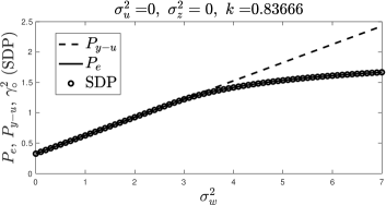
Figure 3: Power spectrum densities $P_{y-u}$ and $P_{e}$ (given by (124)) and the optimal value of the SDP problem (81)–(87) for a range of $\sigma_{w}^{2}$, for the beam splitter transmittance of $\eta=0.7$.

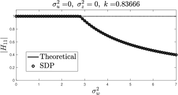
Figure 4: The theoretical (equation (120)) and numerically obtained (via the SDP problem (81)–(87)) optimal gains $|H_{11}|$ for a range of $\sigma_{w}^{2}$, for the beam splitter transmittance of $\eta=0.7$.

For this comparison, consider a quantum-mechanical beam splitter as a special case of a static two-input two-output quantum channel. In this case, $k=\sqrt{\eta}$, $m=\sqrt{1-\eta}$, where $\eta\in(0,1)$ is the transmittance of the device. That is, $y=\sqrt{\eta}u+\sqrt{1-\eta}w$.

Figure 3 shows the plot of the optimal value of the LMI problem (88)–(94) obtained for this example numerically. Since the parameters of the system are constant w.r.t. $\omega$, interpolation is not required in this example, and one can use the obtained numerical value $H_{11}$ directly to obtain an optimal equalizer, as was done in Proposition 2. The optimal $H_{11}$ obtained numerically is real, the graph of the optimal $|H_{11}|$ for this example is shown in Figure 4. For comparison, Figures 3 and 4 also show the graphs of the optimal $P_{e}$ in equation (124) and the optimal gain $H_{11}$ obtained in Proposition 2. Remarkably, both the graphs of the optimal value of the optimization problem and the graphs of the optimal gain are essentially identical.

The threshold on the intensity of the noise $w$ separating the two alternative equalization strategies can also be seen vividly in the graphs. With the chosen parameters, the threshold is $\bar{\sigma}_{w}^{2}=\frac{(1+\sigma_{u}^{2})\sqrt{\eta}-\sigma_{u}^{2}\eta}{1-\eta}$. When $\sigma_{w}^{2}$ is below this threshold, the equalizing filter is given by (122), and we let $H_{22}(s)=1$:

$$\hat{u}=y=\sqrt{\eta}u+\sqrt{1-\eta}w.$$

I.e., the optimal equalization policy is to pass the channel output $u$ unaltered. On the other hand, when $\sigma_{w}^{2}>\bar{\sigma}_{w}^{2}$, the optimal equalizing filter is given by (123). Letting $U_{12}=U_{21}=1$ yields the following expression for the mean-square optimal estimate of $u$,

$$\hat{u} = \frac{(1+\sigma_{u}^{2})\eta}{\psi}u+\frac{(1+\sigma_{u}^{2})\sqrt{\eta}\sqrt{1-\eta}}{\psi}w$$

$$+\frac{1}{\psi}\sqrt{\psi^{2}-(1+\sigma_{u}^{2})^{2}\eta}z.$$

When $\sigma_{w}^{2}>\bar{\sigma}_{w}^{2}$, $\frac{(1+\sigma_{u}^{2})\sqrt{\eta}\sqrt{1-\eta}}{\psi}<\sqrt{1-\eta}$, i.e., the optimal filter applies a reduced gain to the input $w$, compared with the gain $\sqrt{1-\eta}$ of the corresponding term in the expression for $y$. This results in the lower intensity of the filtering error; see Figure 3. The figure confirms that when the intensity of the thermal noise $w$ is sufficiently large, the optimal equalizer is able to reduce the degrading effect of the auxiliary noise $w$ by trading it for a smaller intensity noise injected through the channel $z$. On the contrary, when the noise $w$ has low intensity, such trade-off is not possible, and the filter resorts to passing the channel output $y$ through without any modification.

We conclude the example by pointing out that for a beam splitter of transmittance $\eta$, the optimal equalizer (123) can be implemented using a single beam splitter with the transmittance $\frac{(1+\sigma_{u}^{2})^{2}\eta}{(\sigma_{u}^{2}\eta+\sigma_{w}^{2}(1-\eta))^{2}}$. I.e., the optimal channel-equalizer system has the configuration shown in Fig. 1.

6.2 Equalization of an optical cavity system

Guaranteed cost equalization

[width=0.9]cavity-simplified-marked

Figure 5: A cavity, beam splitters and an equalizer system.

Consider the equalization system shown in Fig. 5. The channel consists of an optical cavity and two optical beam splitters. As in the previous example, the input fields $u$ and $w$ are scalar. For simplicity, suppose that the transmittance parameters $k_{1}^{2}$, $k_{2}^{2}$ of the beam splitters are equal, and that $k_{1},k_{2}$ are real positive numbers, and so $k_{1}=k_{2}=k$ is a real constant. Thus, the relations between the input and output fields of the beam splitters are

$$\left[\begin{array}[]{c}u_{1}\\ w_{1}\end{array}\right]=\left[\begin{array}[]{cc}k&m\\ -m&k\end{array}\right]\left[\begin{array}[]{c}u\\ w\end{array}\right],\quad\left[\begin{array}[]{c}y\\ d\end{array}\right]=\left[\begin{array}[]{cc}k&m\\ -m&k\end{array}\right]\left[\begin{array}[]{c}u_{2}\\ w_{2}\end{array}\right],$$

$m=\sqrt{1-k^{2}}$. The transfer function of the optical cavity is $G_{c}(s)=\frac{s-\kappa+i\Omega}{s+\kappa+i\Omega}$, $\kappa>0$, $\Omega$ are real numbers, i.e., $u_{2}=G_{c}(s)u_{1}$. Then the elements of the transfer function $G(s)$ of the channel are

$$G_{11}(s) = k^{2}G_{c}(s)-(1-k^{2}),$$

$$G_{12}(s) = k\sqrt{1-k^{2}}(G_{c}(s)+1),$$

$$G_{21}(s) = -k\sqrt{1-k^{2}}(G_{c}(s)+1),$$

$$G_{22}(s) = k^{2}-(1-k^{2})G_{c}(s).$$ (130)

Our standing assumptions in this section are that $\sigma_{w}^{2}>\sigma_{u}^{2}>0$ and $k^{2}<\frac{1}{2}$. Under these assumptions,

$$\rho\triangleq 1+\frac{\sigma_{u}^{2}}{2(\sigma_{w}^{2}-\sigma_{u}^{2})k^{2}(1-k^{2})}>1,\quad\hat{\rho}\triangleq\frac{\rho-1}{\rho+1}\in(0,1),$$

$$\delta\triangleq\frac{\sqrt{1-k^{2}}}{k}>1,\quad\hat{\delta}\triangleq\frac{\delta^{2}+1}{\delta^{2}-1}=\frac{1}{1-2k^{2}}>1.$$ (131)

From (4), we have

$$\Upsilon_{3}=\sqrt{\sigma_{u}^{2}+2-\gamma^{2}}>0.$$ (132)

In the next proposition, the following notation will be used:

$$\beta \triangleq \frac{1+\sigma_{u}^{2}}{\Upsilon_{3}\sqrt{2(\sigma_{w}^{2}-\sigma_{u}^{2})(1+\rho)}}(\delta-\frac{1}{\delta}),$$

$$\alpha \triangleq \sqrt{\beta^{2}-1},\quad\nu\triangleq\sqrt{\beta^{2}\hat{\delta}^{2}-\hat{\rho}},$$ (133)

$$\mu \triangleq \sqrt{2(\sigma_{w}^{2}-\sigma_{u}^{2})k^{2}(1-k^{2})(1+\rho)},$$

$$N_{1}(s) = \beta(s+i\Omega)+\beta\hat{\delta}\kappa,$$

$$N_{2}(s) = \alpha(s+i\Omega)+\nu\kappa.$$

Proposition 4.

Suppose $\gamma$ is chosen so that $\beta>1$ and $\gamma^{2}<\sigma_{u}^{2}+2$. Then $H_{11}(s)\in\mathscr{H}_{11,\gamma}$ if and only if

$$H_{11}(s) = -\frac{\Upsilon_{3}}{\mu}\frac{s+\kappa+i\Omega}{N_{1}(s)-\Theta(s)N_{2}(s)},$$ (134)

where $\Theta(s)$ is a stable rational transfer function analytic in the closed right half-plane, which satisfies $\|\Theta\|_{\infty}<1$ and the frequency domain condition

$$\left|\frac{N_{1}(i\omega)-\Theta(i\omega)N_{2}(i\omega)}{i(\omega+\Omega)+\kappa}\right|\geq\frac{\Upsilon_{3}}{\mu}\quad\forall\omega\in\mathbf{R}.$$ (135)

Proof: Using the notation in (131), the function $\Psi(s)$ given in equation (38) is expressed as

$$\Psi(s) = \sigma^{2}_{u}+2(\sigma_{w}^{2}-\sigma_{u}^{2})k^{2}(1-k^{2})\left(1+\frac{(s+i\Omega)^{2}+\kappa^{2}}{(s+i\Omega)^{2}-\kappa^{2}}\right)$$

$$= 2(\sigma_{w}^{2}-\sigma_{u}^{2})k^{2}(1-k^{2})(1+\rho)\frac{(s+i\Omega)^{2}-\hat{\rho}\kappa^{2}}{(s+i\Omega)^{2}-\kappa^{2}}.$$

Clearly, $\Psi(s)$ has full normal rank. It admits the spectral decomposition (58) with the spectral factor

$$M(s)=\mu\frac{s+\kappa\sqrt{\hat{\rho}}+i\Omega}{s+\kappa+i\Omega}.$$ (136)

Both $M(s)$ and $M^{-1}(s)$ are stable and analytic in the half-plane $\mathrm{Re}s>-\kappa\sqrt{\hat{\rho}}$. Using (136), the transfer function $Q(s)$ in (66) is expressed as

$$Q(s)=\frac{1+\sigma_{u}^{2}}{\sqrt{2(\sigma_{w}^{2}-\sigma_{u}^{2})(1+\rho)}}(\delta-\frac{1}{\delta})\frac{s+\hat{\delta}\kappa+i\Omega}{s+\kappa\sqrt{\hat{\rho}}+i\Omega}.$$

Using this information, one can readily check that the matrix $\Upsilon(s)$ in which

$$\Upsilon_{1}(s) = \frac{N_{1}(s)}{s+\sqrt{\hat{\rho}}\kappa+i\Omega}=\beta\frac{s+\hat{\delta}\kappa+i\Omega}{s+\sqrt{\hat{\rho}}\kappa+i\Omega},$$

$$\Upsilon_{2}(s) = \frac{N_{2}(s)}{s+\sqrt{\hat{\rho}}\kappa+i\Omega}=\alpha\frac{s+\frac{\nu}{\alpha}\kappa+i\Omega}{s+\sqrt{\hat{\rho}}\kappa+i\Omega},$$ (137)

$\Upsilon_{3}$ is defined in (132) and $\Upsilon_{4}=0$, is a $J$-spectral factor of the corresponding matrix $\Phi(s)$. Indeed, when $\beta>1$, the constants $\alpha$ and $\nu$ in (133) are well defined, and the identity (67) can be verified directly. Also, since $\sqrt{\hat{\rho}}\kappa>0$, $\Upsilon_{1}(s)$ and $\Upsilon_{2}(s)$ are stable and are analytic in the half-plane $\mathrm{Re}(s)>-\sqrt{\hat{\rho}}\kappa$. Therefore, $\Upsilon(s)$ also has these properties. Similarly, since $\hat{\delta}$ is positive, then $\Upsilon_{1}(s)^{-1}$ is also stable and is analytic in the half-plane $\mathrm{Re}(s)>-\hat{\delta}\kappa$.

Finally, we note that

$$\Upsilon(s)^{-1}=\frac{1}{K(s)}\left[\begin{array}[]{cc}0&-\Upsilon_{2}(s)\\ -\Upsilon_{3}&\Upsilon_{1}(s)\end{array}\right],$$ (138)

where

$$K(s)=\det\Upsilon(s)=-\Upsilon_{3}\Upsilon_{2}(s)=-\Upsilon_{3}\alpha\frac{s+\frac{\nu}{\alpha}\kappa+i\Omega}{s+\sqrt{\hat{\rho}}\kappa+i\Omega}.\quad$$ (139)

Therefore $\frac{1}{K(s)}$ is stable and is analytic in the half-plane $\mathrm{Re}s>-\frac{\nu}{\alpha}\kappa$. Thus we conclude that $\Upsilon(s)^{-1}$ is stable and is analytic in a half-plane $\mathrm{Re}s>-\tau$, $\exists\tau>0$.

These properties verify the conditions of Theorem 3. Therefore $H_{11}(s)\in\mathscr{H}_{11,\gamma}$ if and only if there exists a transfer function $\Theta(s)$ with properties described in that theorem for which $H_{11}(s)$ can be expressed by equation (69).

Since we chose $\Upsilon_{4}=0$, we can use Corollary 2 to obtain the general form of a feasible $H_{11}(s)$. Substituting (136), (137) in (77) yields (134). The frequency domain condition (135) follows from (3) and (4) in the same manner. $\Box$

As in the previous section, it is useful to derive sufficient conditions which would allow us to obtain a $\Theta(s)$ which solves (135). For this, we restrict attention to constant $\Theta$’s.

Corollary 3.

Under the conditions of Proposition 4, if

$$\beta+\alpha>\mu^{-1}\sqrt{\sigma_{u}^{2}+2-\gamma^{2}},$$ (140)

then for any constant $\Theta\in(-1,\min\{\alpha^{-1}(\beta-\mu^{-1}\Upsilon_{3}),0\})$ the corresponding $H_{11}(s)$ given by equation (134) belongs to $\mathscr{H}_{11,\gamma}$.

Proof: For a constant $\Theta$, (135) is equivalent to

$$\frac{\Upsilon_{3}}{\mu}\sqrt{\frac{(\omega+\Omega)^{2}+\kappa^{2}}{(\beta-\Theta\alpha)^{2}(\omega+\Omega)^{2}+(\beta\hat{\delta}-\Theta\nu)^{2}}}\leq 1\quad\forall\omega\in\mathbf{R}.$$

The maximum of the expression on the left-hand side is equal to $\frac{\Upsilon_{3}}{\mu}/\min\{|\beta-\Theta\alpha|,|\beta\hat{\delta}-\Theta\nu|\}$. Therefore, (135) is equivalent to the condition

$$\min\{|\beta-\Theta\alpha|,|\beta\hat{\delta}-\Theta\nu|\}\geq\mu^{-1}\sqrt{\sigma_{u}^{2}+2-\gamma^{2}}.$$ (141)

Next, we show that (141) holds for any $\Theta\in(-1,\min\{\alpha^{-1}(\beta-\mu^{-1}\Upsilon_{3}),0\})$. Indeed, condition (140) guarantees that this interval is not an empty set. Then for any $\Theta$ in that interval,

$$\min\{|\beta-\Theta\alpha|,|\beta\hat{\delta}-\Theta\nu|\}=\beta-\Theta\alpha.$$

This identity holds because $\Theta<0$, $\beta\hat{\delta}>\beta$ and $\nu>\alpha$ due to $\hat{\delta}>1$, $\hat{\rho}<1$. Furthermore, $\Theta<\alpha^{-1}(\beta-\mu^{-1}\Upsilon_{3})$ implies $\beta-\Theta\alpha>\mu^{-1}\Upsilon_{3}.$ This validates (141) and (135). The claim then follows from Proposition 4. $\Box$

Finally, we apply Corollary 3 and Theorem 1 to obtain a complete physically realizable suboptimal equalizer for the cavity system in this example. For convenience, we introduce the additional notation

$$a=-\frac{\Upsilon_{3}}{\mu(\beta-\Theta\alpha)},\quad c=\frac{\beta\hat{\delta}-\Theta\nu}{\beta-\Theta\alpha}.$$ (142)

Conditions of Corollary 3 allow us to select $\Theta\in(-1,\min\{\alpha^{-1}(\beta-\mu^{-1}\Upsilon_{3}),0\})$, i.e., $\Theta<0$ and

$$|a| = \frac{\Upsilon_{3}}{\mu|\beta-\Theta\alpha|}=\frac{\Upsilon_{3}}{\mu(\beta-\Theta\alpha)}<1,$$

$$c = \frac{\beta\hat{\delta}-\Theta\nu}{\beta-\Theta\alpha}>1>|a|.$$

Hence $c^{2}-a^{2}>0$, $1-a^{2}>0$.

Using this notation, the transfer function $H_{11}(s)$ in (134) can be written in a compact form

$$H_{11}(s) = a\frac{s+\kappa+i\Omega}{s+c\kappa+i\Omega}.$$ (143)

Clearly, it satisfies condition (H1) of Theorem 1. The frequency domain condition (135) ensures that condition (H2) is also satisfied. Then we compute

$$X_{1}(s) = X_{2}(s)=1-H_{11}(s)H_{11}(s)^{H}$$ (144)

$$= (1-a^{2})\frac{(s+i\Omega)^{2}-\frac{c^{2}-a^{2}}{1-a^{2}}\kappa^{2}}{(s+i\Omega)^{2}-c^{2}\kappa^{2}}.$$

It is easy to check that $X_{1}(s)$ and $X_{2}(s)$ are para-Hermitian and satisfy condition (H3) of Theorem 1. Let us define the spectral factors of $X_{1}(s)$, $X_{2}(s)$,

$$H_{12}(s) = -\sqrt{1-a^{2}}\frac{s+\sqrt{\frac{c^{2}-a^{2}}{1-a^{2}}}\kappa+i\Omega}{s+c\kappa+i\Omega},$$ (145)

$$\tilde{H}_{21}(s) = -H_{12}(s)=\sqrt{1-a^{2}}\frac{s+\sqrt{\frac{c^{2}-a^{2}}{1-a^{2}}}\kappa+i\Omega}{s+c\kappa+i\Omega},$$

$$\tilde{H}_{21}^{-1}(s) = \frac{1}{\sqrt{1-a^{2}}}\frac{s+c\kappa+i\Omega}{s+\sqrt{\frac{c^{2}-a^{2}}{1-a^{2}}}\kappa+i\Omega},$$

and also select

$$U(s)=\frac{s-\sqrt{\frac{c^{2}-a^{2}}{1-a^{2}}}\kappa+i\Omega}{s+\sqrt{\frac{c^{2}-a^{2}}{1-a^{2}}}\kappa+i\Omega}.$$

This transfer function is paraunitary, stable and analytical in the right half-plane $\mathrm{Re}s>-\sqrt{\frac{c^{2}-a^{2}}{1-a^{2}}}$, as required by Theorem 1. Using these definitions the remaining blocks of $H(s)$ are obtained according to (1):

$$H_{21}(s) = U(s)\tilde{H}_{21}(s)$$

$$= \sqrt{1-a^{2}}\frac{s-\sqrt{\frac{c^{2}-a^{2}}{1-a^{2}}}\kappa+i\Omega}{s+c\kappa+i\Omega},$$

$$H_{22}(s) = -U(s)(\tilde{H}_{21}^{-1}(s))^{H}H_{11}(s)^{H}H_{12}(s)$$ (146)

$$= a\frac{s-\kappa+i\Omega}{s+c\kappa+i\Omega}.$$

The following proposition which follows from Theorem 1 summarizes our analysis.

Proposition 5.

Given a constant $\gamma$ which satisfies the conditions of Proposition 4 and Corollary 3, consider the transfer function $\Xi(s)=\Delta(H(s),0)$ where $H(s)$ is composed of the blocks defined in equations (143), (145) and (6.2); see (21). Then $\Xi(s)=\Delta(H(s),0)$ is a passive physically realizable stable and causal guaranteed cost equalizer for the cavity system under consideration, and

$$\sup_{\omega}P_{e}(i\omega,\Xi)<\gamma^{2}.$$ (147)

It is worth pointing out that the guaranteed cost equalizer in this example can be realized using an interconnection of an optical cavity and two beam splitters shown in Figure 6. The transfer function of the optical cavity in the figure is

$$y_{2}=H_{c}(s)y_{1},\quad H_{c}(s)=\frac{s-c\kappa+i\Omega}{s+c\kappa+i\Omega},$$

and the beam splitters’ operators are

$$\left[\begin{array}[]{c}y_{1}\\ z_{1}\end{array}\right]=\left[\begin{array}[]{cc}\xi_{1}&\eta_{1}\\ \eta_{1}&-\xi_{1}\end{array}\right]\left[\begin{array}[]{c}y\\ z\end{array}\right],\quad\left[\begin{array}[]{c}\hat{u}\\ \hat{z}\end{array}\right]=\left[\begin{array}[]{cc}\eta_{2}&\xi_{2}\\ \xi_{2}&-\eta_{2}\end{array}\right]\left[\begin{array}[]{c}y_{2}\\ z_{2}\end{array}\right],$$

where

$$\eta_{1}=-\sqrt{\frac{c+a^{2}-\sqrt{(c^{2}-a^{2})(1-a^{2})}}{2c}},$$

$$\xi_{1}=\sqrt{1-\eta_{1}^{2}}=\sqrt{\frac{c-a^{2}+\sqrt{(c^{2}-a^{2})(1-a^{2})}}{2c}},$$

$$\eta_{2}=-\sqrt{\frac{c-a^{2}-\sqrt{(c^{2}-a^{2})(1-a^{2})}}{2c}},$$

$$\xi_{2}=\sqrt{1-\eta_{2}^{2}}=\sqrt{\frac{c+a^{2}+\sqrt{(c^{2}-a^{2})(1-a^{2})}}{2c}}.$$

[width=0.7]cavity-filter

Figure 6: A cavity and beam splitters realization of the equalizer.

Proposition 5 reduces the question of finding a suboptimal physically realizable equalizer to checking whether (140) is satisfied for a given $\gamma$ such that $\gamma<\sigma_{u}^{2}+2$ and $\beta>1$. It is also possible to minimize the upper bound $\gamma^{2}$ on $\sup_{\omega}P_{e}(i\omega,\Xi)$ over the set $\{\gamma\colon\gamma^{2}\in(0,\sigma_{u}^{2}+2),\beta>1,\beta+\alpha>\mu^{-1}\Upsilon_{3}\}$. This will lead to a suboptimal solution to the problem. Figure 7 illustrates this. The solid line in Figure 7 shows such a suboptimal $\gamma^{2}$ obtained for a range of values of $\sigma_{w}^{2}>\sigma_{u}^{2}$, where $\sigma_{u}^{2}=0.1$, $k=0.4$, $\kappa=5$, $\Omega=10$.

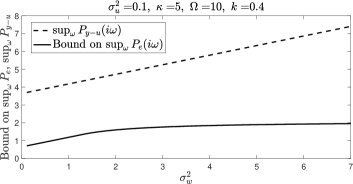
Figure 7: $\sup_{\omega}P_{y-u}(i\omega)$ (the dash line) and the optimized bound on $\sup_{\omega}P_{e}(i\omega)$ (the solid line) for a range of $\sigma_{w}^{2}$, for an optical cavity.

For comparison, the figure shows the graph of the error power spectrum density $\sup_{\omega}P_{y-u}$ of the system without an equalizer (the dashed line). The advantage of equalization is quite clear from this figure. Fig. 8 shows the Bode plot of one of the suboptimal transfer functions $H_{11}(s)=-\frac{s+5+10i}{s+7.961+10i}$ obtained for the cavity system with $\sigma_{w}^{2}=0.2$. It confirms that $|H_{11}(i\omega)|<1$.

Figure 8: The Bode plot of one of the suboptimal transfer functions $H_{11}(s)$ obtained using equation (134) with $\Theta=-0.9998$. The parameters of the system are $\sigma_{w}^{2}=0.2$, $\sigma_{u}^{2}=0.1$, $k=0.4$, $\kappa=5$, $\Omega=10$.

Equalization via semidefinite programming

We now illustrate the application of the approximation technique presented in Section 5. For this, we consider the same cavity system with parameters $k=0.4$, $\kappa=5$, $\Omega=10$, $\sigma_{w}^{2}=0.2$, $\sigma_{u}^{2}=0.1$. Recall that the transfer function matrix $G(s)$ of that system is a $2\times 2$ matrix, its elements are given in (6.2).

To apply the algorithm described in Section 5 to this system, first a set of $L=21$ points $\omega_{l}$ was selected which included $0$, ten logarithmically spaced frequency points in the interval $[10^{-3},10]$ and the corresponding negative frequencies. With these data, the LMI problem (88)–(94) was solved numerically and the array of values $H_{11,l}$ was obtained, $l=1,\ldots,L$, along with the value of the optimization problem. In this example, this value was obtained to be $\tilde{\gamma}^{2}=0.7049$. It is worth noting that $\tilde{\gamma}^{2}<\sigma_{u}^{2}+2$; this validates (55). This set of data was then used to solve the Nevanlinna-Pick interpolation problem.

The procedure outlined in Section 5 involves mapping the half-plane $\mathrm{Re}s>-\tau$ conformally onto the half-plane $\mathrm{Re}s>0$, performing interpolation over this half-plane to obtain $\hat{H}_{11}(s)$, then obtaining $H_{11}(s)$ via (104). To implement this procedure, we used the conformal mapping $s^{\prime}=s+\tau$, where we let $\tau=10^{-3}$. This ensured that the grid points $i\omega_{l}$ on the imaginary axis were mapped conformally into the interior of the right half-plane $\mathrm{Re}s>0$, as required by the algorithm in Section 5.

Theorem NP in [15] allows to obtain a solution using (96), provided the Pick matrix $\mathbf{P}$ is positive definite. This assumption of the Nevanlinna-Pick interpolation theory was satisfied in this example.

The method gives the analytical expression (96) for $\hat{H}_{11}(s)$. Since it involves inverting the Pick matrix $\mathbf{P}$, a closed form expression for (96) is quite cumbersome, even when a modest number of grid points is selected. Therefore we validated our approach numerically. For this, we selected additional grid points on the imaginary axis, while keeping the original frequencies as a control set. Then we computed interpolated values of $H_{11}(i\omega)$ at those grid points, using (96), (104) with $\Theta(s)=-0.95,0$ and $0.95$. Also, the corresponding normalized values of the error power spectrum density, $P_{e}(i\omega,H_{11})/{\tilde{\gamma}^{2}}$, were computed. The graphs of these quantities are shown in Fig. 9(a) using solid lines.

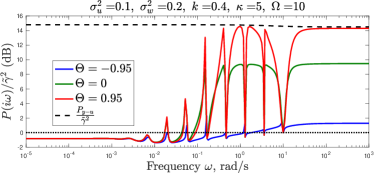
(a)

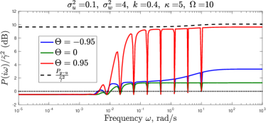
(b)

Figure 9: The normalized computed error power spectrum densities $P_{e}/{\tilde{\gamma}^{2}}$ (the solid lines) and the normalized error $P_{y-u}/{\tilde{\gamma}^{2}}$ (the dash line): (a) $\sigma_{w}^{2}=0.2$; (b) $\sigma_{w}^{2}=4$.

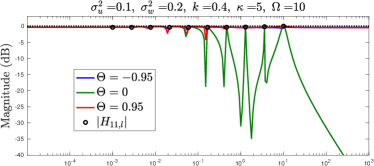
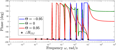
(a)

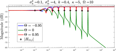
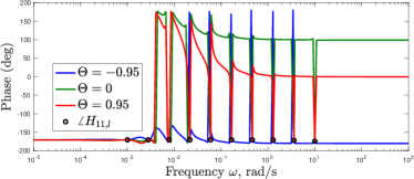
(b)

Figure 10: The Bode plots of $H_{11}(s)$ for $\Theta=-0.95,0$ and $0.95$. The circles indicate the magnitude and phase of $H_{11,l}$ obtained from the optimization problem (88)–(94): (a) $\sigma_{w}^{2}=0.2$; (b) $\sigma_{w}^{2}=4$.

Fig. 10(a) confirms that all three computed $H_{11}(i\omega)$ agree at the grid frequencies. The sharp peaks in the graphs occur at the grid point frequencies $\omega_{l}$ which were used in the LMIs (91), (94). These peaks occur because the transfer functions $W_{ij}(s)$ which parameterize the solution have poles at $-\tau+i\omega_{l}$; see (103). When $\tau=0.001$, these poles are quite close to the imaginary axis.

Other than at the control frequencies $\omega_{l}$, all three graphs of $P_{e}(i\omega,H_{11})$ deviate from the optimal value $\tilde{\gamma}^{2}$ of the problem (88)–(94). This is expected since the algorithm optimizes the PSD of the error at selected frequency points only. It is worth noting that away from the grid frequencies, $P_{e}(i\omega,H_{11})$ varies considerably, depending on $\Theta$. When we let $\Theta=-0.95$ in (96), interpolation led to a substantially improved error power spectrum density, in comparison with the power spectrum density $P_{y-u}(i\omega)$ of the difference $y-u$. However, when $\Theta=0.95$, the error power spectrum density deviated considerably from the value $\tilde{\gamma}^{2}$, and was relatively close to $P_{y-u}(i\omega)$. Nevertheless, the observed reduction of the error PSD using $\Theta=-0.95$ and $\Theta=0$ indicates that there is room for further optimization of $P_{e}(i\omega,H_{11})$ over the parameter $\Theta(s)$. Simulations performed with other values of $\sigma_{w}^{2}$ (e.g., see Fig. 9(b) and 10(b)) confirmed this finding. This interesting problem will be addressed in future research.

Another interesting observation is that with the selected parameters, the optimization problem (88)-(94) produced a set of points $H_{11,l}$ that were quite close to the boundary of the set $|H_{11}(i\omega)|\leq 1$. As a result, while all three interpolants satisfied the constraint (53) of Problem 1’ required for physical realizability of the filter, they do so with a rather small margin; see Fig. 10(a). The intuition gained in the previous section suggests that when the noise intensity is sufficiently large, the parameter $H_{11}$ of the filter should reduce away from the boundary of the constraint set, in an attempt to reduce the contribution of the noise field to the output of the equalizer. This is confirmed in Fig. 10(b), which illustrates the results of interpolation when $\sigma_{w}^{2}=4$. This time all obtained $H_{11,jl}$ have magnitude of order of 0.4. The corresponding value $\tilde{\gamma}^{2}=1.8117$.

It is worth noting that for both values of $\sigma_{w}^{2}$, letting $\Theta=0$ led to $H_{11}(i\omega)$ vanishing at large $\omega$. When $\sigma_{w}^{2}=0.2$, the filter with $H_{11}(s)$ that vanishes as $\omega\to\infty$ is not mean-square optimal. However, when $\sigma_{w}^{2}=4$, the equalizer with $\Theta=0$ is the best out of the three in terms of performance. In this equalizer, the gain $H_{12}(i\omega)$ dominates $H_{11}(i\omega)$ as $\omega\to\infty$. An explanation to this is that when the intensity of the channel noise field becomes very large, from the view point of optimizing the mean-square error, it becomes advantageous to block high frequency components of the channel output altogether and transfer the filter environment field as the filter output. Such a filtering strategy may not be beneficial when the information accuracy of the system is important — despite the signal-to-noise ratio is low, the noisy channel output still carries some information about its input, while the filter environment does not carry such information. Therefore, an interesting problem for future research is to find a trade-off between mean-square accuracy and information accuracy of coherent equalizers, similar to the problem considered recently for classical Kalman-Bucy filters [24].

7 Conclusions

The paper has introduced a quantum counterpart of the classical equalization problem. The discussion is focused on passive quantum channels and passive quantum filters, and is motivated by the utility and the ease of implementation of passive quantum systems [18, 20].

Different from the previous work on developing coherent Wiener and Kalman filters, we posed the quantum equalization problem in the same vein as the classical $H_{\infty}$ filtering problem. However, instead of the disturbance-to-error transfer function, we considered the PSD of the difference between the input field of the quantum communication channel and the output field of the equalizer as the measure of the equalizer performance. Accordingly, the filter was sought to guarantee that the maximum eigenvalue of the error PSD was below a prescribed threshold. The requirement that such filter must be physically realizable, adds a constraint on the filter.

We have shown that this problem reduces to a constrained optimization with respect to one of the blocks of equalizer’s transfer function matrix. Using the $J$-spectral factorization technique, we have developed a convenient parameterization of the class of suboptimal filters similar to the Youla parameterization of the class of stabilizing controllers.

Also, this auxiliary problem was cast as a semidefinite program subject to frequency-dependent linear matrix inequality constraints, and a tractable constraint relaxation was proposed involving constraints over a discrete set of frequencies. In addition, the Nevanlinna-Pick interpolation technique was employed to ensure that the solution to the relaxed problem yields a physically realizable filter. A set of all interpolating filters was also obtained. In principle, coherent filters obtained this way are not guaranteed to yield an improved mean-square performance over the entire interval of frequencies. Therefore it is interesting to attempt to minimize the error power spectrum density over the set of interpolating filters. Another possible direction for future research is to find a trade-off between mean-square accuracy and information accuracy of coherent equalizers.

The paper gives two examples of equalization of single mode channels. One of them comprises a static quantum system as a channel, and another one includes a quantum optical cavity. These examples demonstrate that coherent equalizers can be effective in improving the mean-square accuracy of the channel. We also showed that in the static case, passive equalizers are especially beneficial when the intensity of the thermal noise from the channel environment exceeds certain threshold. A linear matrix inequality condition has been introduced to predict such a threshold in a general case.

References

• [1] J. Ball, I. Gohberg, and L. Rodman. Interpolation of rational matrix functions. Birkhäuser, Basel, 1990.
• [2] T. N. Davidson, Z.-Q. Luo, and J. F. Sturm. Linear matrix inequality formulation of spectral mask constraints with applications to FIR filter design. IEEE Transactions on Signal Processing, 50(11):2702–2715, 2002.
• [3] P. Delsarte, Y. Genin, and Y. Kamp. The Nevanlinna-Pick problem for matrix-valued functions. SIAM Journal on Applied Mathematics, 36(1):47–61, 1979.
• [4] D. G. Feingold and R. S. Varga. Block diagonally dominant matrices and generalizations of the Gerschgorin circle theorem. Pacific Journal of Mathematics, 12(4):1241–1250, 1962.
• [5] B. A. Francis and J. C. Doyle. Linear control theory with an $\mathbf{H}_{\infty}$ optimality criterion. SIAM Journal on Control and Optimization, 25(4):815–844, 1987.
• [6] T. T. Georgiou and P. P. Khargonekar. Spectral factorization of matrix-valued functions using interpolation theory. IEEE Transactions on Circuits and Systems, 36(4):568–574, 1989.
• [7] J. E. Gough, M. R. James, and H. I. Nurdin. Squeezing components in linear quantum feedback networks. Physical Review A, 81(2):023804, 2010.
• [8] M. Green, K. Glover, D. Limebeer, and J. Doyle. A ${J}$-spectral factorization approach to $\mathscr{H}_{\infty}$ control. SIAM Journal on Control and Optimization, 28(6):1350–1371, 1990.
• [9] B. Hassibi, A. H. Sayed, and T. Kailath. Indefinite-quadratic estimation and control: A unified approach to $H^{2}$ and $H^{\infty}$ theories. SIAM, Philadelphia, 1999.
• [10] R. A. Horn and F. Zhang. Basic properties of the Schur complement. In The Schur Complement and Its Applications, pages 17–46. Springer, 2005.
• [11] R. L. Hudson and K. R. Parthasarathy. Quantum Ito’s formula and stochastic evolutions. Communications in Mathematical Physics, 93(3):301–323, 1984.
• [12] V. Ionescu and C. Oara. The four-block Nehari problem: A generalized Popov-Yakubovich-type approach. IMA Journal of Mathematical Control and Information, 13(2):173–194, 1996.
• [13] M. R. James, H. I. Nurdin, and I. R. Petersen. ${H}^{\infty}$ control of linear quantum stochastic systems. IEEE Transactions on Automatic Control, 53(8):1787–1803, 2008.
• [14] M.R. James and J.E. Gough. Quantum dissipative systems and feedback control design by interconnection. IEEE Transactions on Automatic Control, 55(8):1806 –1821, 2010.
• [15] I. V. Kovalishina. Analytic theory of a class of interpolation problems. Mathematics of the USSR-Izvestiya, 22(3):419–463, 1984.
• [16] A. I. Maalouf and I. R. Petersen. Bounded real properties for a class of annihilation-operator linear quantum systems. IEEE Transactions on Automatic Control, 56(4):786–801, 2011.
• [17] A. I. Maalouf and I. R. Petersen. Coherent ${H}^{\infty}$ control for a class of annihilation operator linear quantum systems. IEEE Transactions on Automatic Control, 56(2):309–319, 2011.
• [18] H. I. Nurdin. On synthesis of linear quantum stochastic systems by pure cascading. IEEE Transactions on Automatic Control, 55(10):2439–2444, 2010.
• [19] H. I. Nurdin, M. R. James, and I. R. Petersen. Coherent quantum LQG control. Automatica, 45(8):1837–1846, 2009.
• [20] H. I. Nurdin and N. Yamamoto. Linear Dynamical Quantum Systems. Springer, 2017.
• [21] K. R. Parthasarathy. An introduction to quantum stochastic calculus. Birkhäuser, 2012.
• [22] A. J. Shaiju and I. R. Petersen. A frequency domain condition for the physical realizability of linear quantum systems. IEEE Transactions on Automatic Control, 57(8):2033–2044, 2012.
• [23] U. Shaked. $H_{\infty}$-minimum error state estimation of linear stationary processes. IEEE Transactions on Automatic Control, 35(5):554–558, 1990.
• [24] T. Tanaka, V. Zinage, V. Ugrinovskii, and M. Skoglund. Continuous-time channel gain control for minimum-information Kalman-Bucy filtering. arXiv:2202.02880.
• [25] V. Ugrinovskii and M. R. James. Active versus passive coherent equalization of passive linear quantum systems. In Proc. 58th IEEE CDC, Nice, France, December 2019. arXiv:1910.06462.
• [26] V. Ugrinovskii and M. R. James. Wiener filtering for passive linear quantum systems. In American Control Conference, Philadelphia, PA, July 10-12 2019. arXiv:1901.09494.
• [27] I. G. Vladimirov and I. R. Petersen. Coherent quantum filtering for physically realizable linear quantum plants. In 2013 European Control Conference (ECC), pages 2717–2723, 2013.
• [28] S. L. Vuglar and I. R. Petersen. How many quantum noises need to be added to make an LTI system physically realizable? In 2011 Australian Control Conference, pages 363–367, 2011.
• [29] N. Wiener. The extrapolation, interpolation, and smoothing of stationary time series. Wiley, New York, 1949.
• [30] S.-P. Wu, S. Boyd, and L. Vandenberghe. FIR filter design via spectral factorization and convex optimization. In Applied and Computational Control, Signals, and Circuits, pages 215–245. Springer, 1999.
• [31] K. Yosida. Functional Analysis. Springer-Verlag, Berlin, Göttingen, Heidelberg, 1965.
• [32] D Youla. On the factorization of rational matrices. IRE Transactions on Information Theory, 7(3):172–189, 1961.
• [33] C.-Y. Zhang, S. Luo, A. Huang, and C. Xu. The eigenvalue distribution of block diagonally dominant matrices and block H-matrices. The Electronic Journal of Linear Algebra, 20:621–639, 2010.
• [34] G. Zhang and M. R James. On the response of quantum linear systems to single photon input fields. IEEE Transactions on Automatic Control, 58(5):1221–1235, 2013.
• [35] K. Zhou, J. C. Doyle, and K. Glover. Robust and optimal control. Prentice Hall, New Jersey, 1996.