[1]
[style=chinese]
Hierarchical Clustering in Astronomy
Abstract
Hierarchical clustering is a common algorithm in data analysis. It is unique among many clustering algorithms in that it draws dendrograms based on the distance of data under a certain metric, and group them. It is widely used in all areas of astronomical research, covering various scales from asteroids and molecular clouds, to galaxies and galaxy cluster. This paper systematically reviews the history and current status of the development of hierarchical clustering methods in various branches of astronomy. These applications can be grouped into two broad categories, one revealing the intrinsic hierarchical structure of celestial systems and the other classifying large samples of celestial objects automatically. By reviewing these applications, we can clarify the conditions and limitations of the hierarchical clustering algorithm, and make more reasonable and reliable astronomical discoveries.
keywords:
hierarchical clustering \sepdendrogram \septaxonomy \sepgravitational system \sephierarchical universe1 Introduction
The classification of data according to their different properties is a basic strategy of scientific research. With the progress of research techniques, these classification methods are gradually abstracted to form a specialized field – cluster analysis (Everitt et al., 2011). Most of the classification and grouping work in astronomy can find corresponding algorithms in this field (Babu and Feigelson, 1996; Ivezić et al., 2014). Emerging techniques in this field are also often borrowed and developed by astronomers.
Hierarchical clustering, or hierarchical cluster analysis (HAC) is such a data analysis algorithm. It is to quantify the distance (or similarity) between data according to some predefined metric, and use dendrogram to present these distances and reveal hierarchical relationships. In 1948, Danish botanist Sørensen (1948) proposed the original form of this algorithm. After years of exploration and improvement by many researchers, a mature hierarchical clustering algorithm has been developed (Lance and Williams, 1967; Gordon, 1987). It does not require users to restrict a priori properties, such as the number of clusters and distribution functions of the sample in advance. So it is an unsupervised learning algorithm in the field of machine learning. The unique advantage of hierarchical clustering is that it does not only provide the final grouping results like other algorithms, but also organizes all the data in a dendrogram that can preserve the complete hierarchy and clustering relationships between data. It gives users the opportunity to select appropriate groups of features from the dendrogram based on different thresholds, and it preserves the associations between the groups.
The universe is hierarchical, because similar organized structures can be seen at different cosmic scales, as stars converge into clusters and galaxies, galaxies form galaxy clusters, and galaxy clusters are interconnected to form the large-scale structure of the universe. Although their spatial scales are very different, their formation and evolution are all dominated by gravity, and they have a similar hierarchical structure, which is suitable for graphical presentation. Hierarchical clustering caught the attention of astronomers as early as 1978, French astronomer Materne introduced it into the field of astronomy, to figure galaxy groups in nearby galaxies (Materne, 1978). Later, this algorithm has been widely used in all branches of astronomy.
This paper systematically introduces the history and current status of the development of hierarchical clustering algorithms in different application scenarios in the field of astronomy. In Section 2, we describe the basic concepts and steps of algorithms; in Section 3, we specifically describe the application of the algorithm in different research branches; Finally, we summarize and discuss its current status and development prospects.
2 Algorithm
The hierarchical cluster analysis have two approaches: one is the "bottom-up" agglomerative method, and the other is the "up-bottom" divisive method. The former starts from a single point of data and merges adjacent points step by step according to a given rule until all data points are combined into one class. While the latter is to treat the whole data set as a whole first and partition it according to certain rules until all data points are separated from each other. These two pathways are mutually inverse operations, and the dendrogram obtained under the same rules are the same. Because that agglomerative hierarchical clustering is more commonly used, it is used as an example below.
2.1 Steps
The main steps of agglomerative hierarchical clustering are as follows:
-
(a)
First, each data point is treated as a set, and the distance between sets is calculated according to a specific metric;
-
(b)
Find the two sets with the smallest distance according to a specific linkage, merge them into a new set, and recalculate the distance between sets. Repeat this step until only one set remains;
-
(c)
Draw a dendrogram according to the order in which sets are merged;
-
(d)
Select a suitable trim threshold to obtain the cluster classification from the dendrogram.
During the process, the most critical design is how to define metric and linkage. Common examples usually adopt the simplest Euclidean distance as the metric. But in practical astronomical applications, the data is multidimensional and has different units and scales. It means that simple superposition is not possible. One way is to normalize them to dimensionless data. However, the normalization parameters are equivalent to the weight of data. They need to be chosen carefully according to experience. Even if feasible, they still face the dilemma of lacking a reasonable physical explanation. Therefore, in practical applications, it is crucial to design an appropriate metric based on the specific physical problem and available data.
Second, there are various ways to link sets(Everitt et al., 2011), usually includes:
-
•
Single linkage. The sets to be linked are determined based on the size of the distance between the nearest points of the sets. Because considering only the nearest group of members between sets will merge the whole set preferentially due to the close distance between individual members, the regular shape and distribution of the group cannot be guaranteed. This is known as the chaining effect and is advantageous in detecting irregular structures(Baron, 2019).
-
•
Complete linkage. Determine the set to be joined based on the size of the distance between the farthest points of the sets. By considering only the farthest set of members between sets, the merging hierarchy of the entire set can be severely affected by individual outliers.
-
•
Average linkage. Determines the set to be connected based on the average size of the distances between all points in the set; neutralizes the effect of single-point and full-set connections, tending to produce a uniformly distributed set.
-
•
Median linkage. Determine the set to be connected based on the median size of the distance between all points in the set; close to the effect of the mean connection and less susceptible to individual outliers.
-
•
Centroid linkage. Determine the set to be connected based on the distance between the centroids of the sets.
-
•
Ward linkage. Determine the set to be connected based on the change in variance between the original set and the new set after the connection (Materne, 1978); which can better separate two noisy data sets.
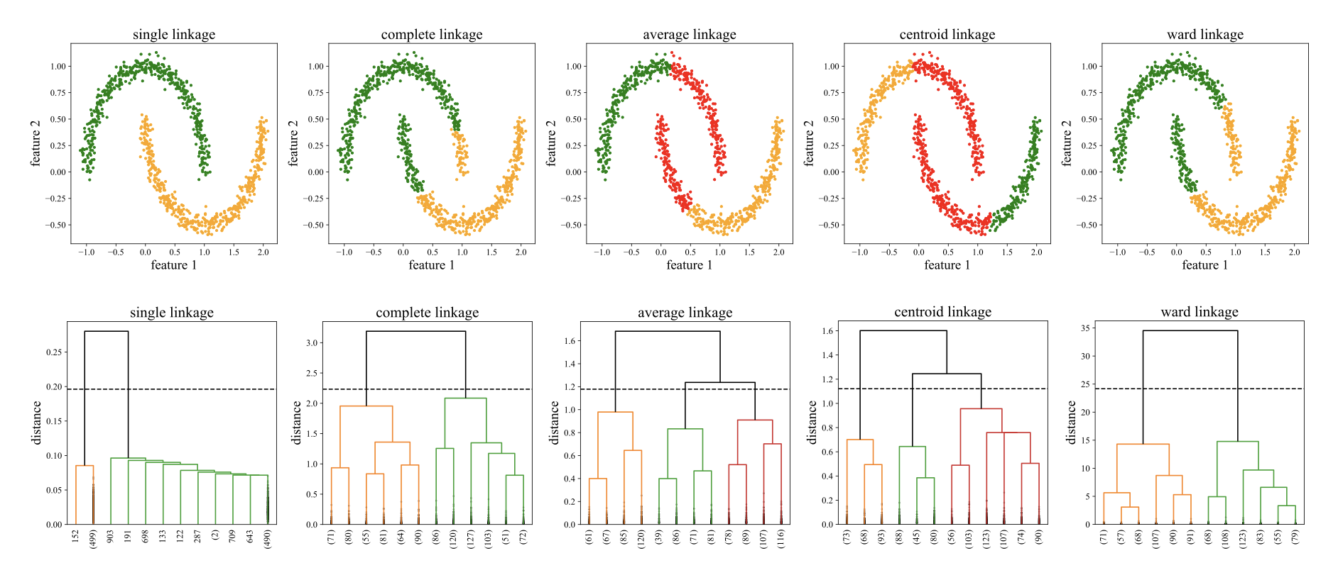
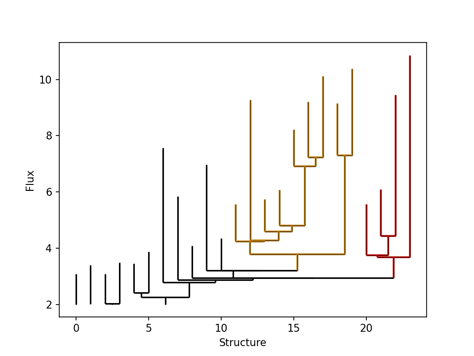
Even with the same metric, different connection methods can lead to very different results, as shown in the Fig.1, which just shows a special case, and should not be taken as a general evaluation of these connections. In fact, these connections are suitable for different scenarios. The selection of the specific connection method needs to be considered in conjunction with the study object characteristics and metric design.
Among these linkage methods, both the single linkage and the complete linkage only need to calculate the distance between two data for one time, the time complexity and space complexity of these two algorithms are (Sibson, 1973; Defays, 1977). But for the average-linkage, median-linkage, centroid-linkage and Ward-linkage, because the distance matrix needs to be updated and stored at each iteration, the time complexity are , and the space complexity are .
With the dendrogram, in principle, the cluster classification can be obtained by choosing a reasonable threshold to trim the tree. Therefore, most of the descriptions of hierarchical clustering in the literature stop at the step of drawing a dendrogram and do not involve the operation of extracting clusters from the tree diagram. In practical applications, clusters are not always clearly visible in the dendrogram. Choosing a reasonable trim threshold is crucial. Manual threshold selection is inevitably influenced by subjective factors such as the user’s empirical preferences. Thus a clear trimming rule is directly related to the stability of results and the automation of the method. However, there is no universal method for trimming dendrograms. They need to be designed according to specific requirements.
2.2 Dendrogram
The signature result of the hierarchical clustering algorithm is the dendrogram. Each node of it is derived from a single set merge operation, include two member branches, thus it is called binary tree in computer science. The node that contains all members is called the root; while the node representing a single original member at the other end is called the leaf. The x-axis position of these leaves in the dendrogram only represent their relative linking sequence. There are multiple topologically equivalent ways of drawing the same dendrogram, which represent exactly the same group relationships. The y-axis of the dendrogram usually uses the generation order of nodes or the metric distance, and it can actually be set flexibly according to actual needs.
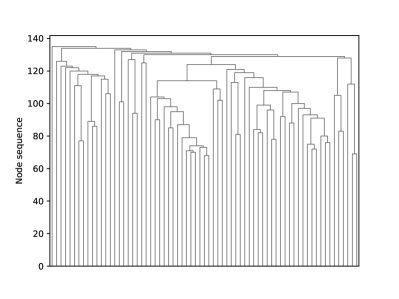
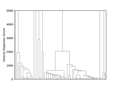
Using different properties as the y axis will make the dendrogram look different. Fig.2 is the dendrogram of optical galaxies in the field view of galaxy cluster MACS0358 (WANG and YU, 2021), plotted with the projection binding between galaxies as the metric(see Section 3.1.1). The upper panel adopts the nodal merger order as the y-axis. It shows the tightness of the gravitational connection between galaxies as it is, but it is difficult to find the trim threshold from it due to the lack of physical meaning. Considering gravitationally-bound galaxy cluster members will exhibit relatively stable values of velocity dispersion, we can adopt the velocity dispersion of the subordinate members of each node as the y-axis (the lower panel of Fig.2). It can visualize the astrophysical properties corresponding to branch nodes. So we can directly use 1000 km s-1, the typical galaxy cluster velocity dispersion, as a threshold to extract physical structures from the dendrogram.
2.3 Procedure
Most mainstream data analysis languages provide related libraries and functions for hierarchical clustering, such as ALGLIB111https://www.alglib.net/dataanalysis/clustering.php of C, Weka222https://www.cs.waikato.ac.nz/ml/weka/ and Hac333http://sape.inf.usi.ch/hac of Java, scipy.cluster.hierarchy and sklearn.cluster 444https://scikit-learn.org/stable/modules/generated/sklearn.cluster.AgglomerativeClustering.html of Python, hclust of R, clusterdata of Matlab, dendro555https://github.com/low-sky/dendro of IDL, etc.
These codes all implement the core function of the algorithm, which can draw the hierarchical tree in different linkage methods. However, in practical applications the analysis and extraction of structures are closely associate with specific physical problems, a lot of additional development work is required on the basis of existing functions. There are specialized packages of hierarchical clustering in astronomy to deal with specific problems. For example, astrodendro 666http://ascl.net/1907.016 – clustering by radio flux of molecular cloud, acorns777http://ascl.net/2003.003 – clustering by radial velocity of molecular cloud, AMANDA888https://ascl.net/1503.006 – clustering by multiple correlation matrix, etc. In researches, we need to select appropriate tools according to our own data characteristics and research goals and modify them.
3 Application
The hierarchical clustering algorithm has a fairly wide applicability because it does not rely on any priori information or models. It has been applied in many fields of astronomy. In the following we review the history and current status of the application of hierarchical clustering methods in different fields.
3.1 Analysis of The Structure of Celestial Bodies
All levels of objects in the universe are clustered by gravity and merge to evolve the hierarchical cosmic structure we see today. In principle, all systems sustained by gravity can be analyzed by hierarchical clustering and presented with a dendrogram.
3.1.1 Galaxy Clusters
As the largest gravitationally-bound system in the universe, galaxy clusters play an important role in the evolution scenario of the universe. On the one hand, they are joints of the large-scale structure; on the other hand, they provide environments for galaxy formation and evolution. The search for galaxy clusters is an important topic. The hierarchical clustering was first introduced to the study of astronomy by Materne (1978) to analyze nearby groups and clusters of galaxies. He designed a dimensionless distance with spatial positions and velocities of galaxies as the metric to explore nearby groups in the Leo region. This attempt made the hierarchical clustering the first astronomical three-dimensional group analysis method. It has attracted the attention of early redshift survey researchers. Tully (1980) tested this algorithm. He designed a quantity related to gravitational force (luminosity divided by the square of the spatial distance) as the distance to analyze the field of galaxy group NGC 1023. In 1987, he designed a density-like metrics to recognize galaxy clusters in the Nearby Galaxies Catalog (Tully, 1987). Gourgoulhon et al. (1992) used a hierarchical clustering algorithm to compile a catalog of all-day galaxy clusters within 80 Mpc of the Milky Way.
Meanwhile, Huchra and Geller (1982) designed a method for processing single linkage results with a fixed threshold to analyze galaxy redshift survey data, as known as the Friend-of-Friend(FoF) algorithm. It corresponds to a fixed level in the hierarchical clustering dendrogram, thus simplifying the computational process and the complexity of operations. Hierarchical clustering and FoF were main group finders at that time. Garcia et al. (1992) systematically compared the differences in galaxy clusters obtained by the two methods. However, due to the lack of an objective and accurate evaluation standard, it is difficult to say which method is more reliable. Garcia (1993) created a galaxy cluster catalog by combining these two methods. Later, FoF algorithm has gradually become a common tool in the astronomical community because of its speed and convenience, and is widely used.
However, there are still researchers who have been persistently exploring the potential of hierarchical clustering for astronomical structure identification. Serna and Gerbal (1996) found when using intergalactic binding energy as a metric, (see equation1), the substructure within galaxy clusters can be visualized on a dendrogram. The typical calculation equation of binding energy as follows:
| (1) |
where G is the gravitational constant, is the star mass, is the pairwise relative distance, is the velocity difference based on spectral redshifts. This is an important breakthrough compared to previous work. As a quantity with a clear physical meaning, binding energy organically combines spatial location and velocity in the data, not only does it solve the problem of scaling the definition of "distance", but the resulting dendrogram is also clearly interpretable. Serna and Gerbal (1996) also found, the dendrogram obtained by single linkage gives the most reasonable results for galaxy clusters detection. There are other work (eg. Adami et al., 2005; Guennou et al., 2014) adopting their method to analyze substructures of clusters. However, their work did not provide a standardized way to trim trees.
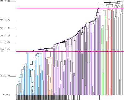
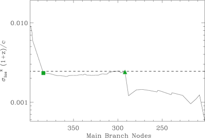
Diaferio (1999) further proposed that the velocity dispersion plateau in the dendrogram could be used to identify the galaxy clusters contained therein. The specific approach is: from the root node, every step moves along the branch with more members, then the main branch of the dendrogram can be obtained. When there is a dominant galaxy cluster in the field, velocity dispersion () from nodes on the main branch will from an obvious plateau as shown in the Fig.3. According to this plateau, the galaxy cluster can be identified in the dendrogram. This procedure provides a quantitative operational standards of structure extraction in dendrogram. Serra and Diaferio (2013) systematically tested this method by using data from large scale cosmological simulations, which confirmed the reliability of it in probing galaxy cluster members.
In fact, this velocity dispersion plateau can be used to detect not only members of galaxy clusters, but also substructures in galaxy clusters. Yu et al. (2015) confirmed this idea through a systematic test of its capabilities in detecting the structure of galaxy clusters using numerical cosmological simulation data. In 2016, they applied this method in galaxy cluster A85, finding an optical substructure moving in the direction of the line of sight in its center, which can well explain the spectral shift of the X-ray gas at the core (Yu et al., 2016). Liu et al. (2018) also applied it to galaxy clusters A2142, confirmed that the substructure given by this method is consistent with the detection by other methods such as X-ray images and weak gravitational lensing.
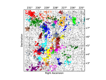
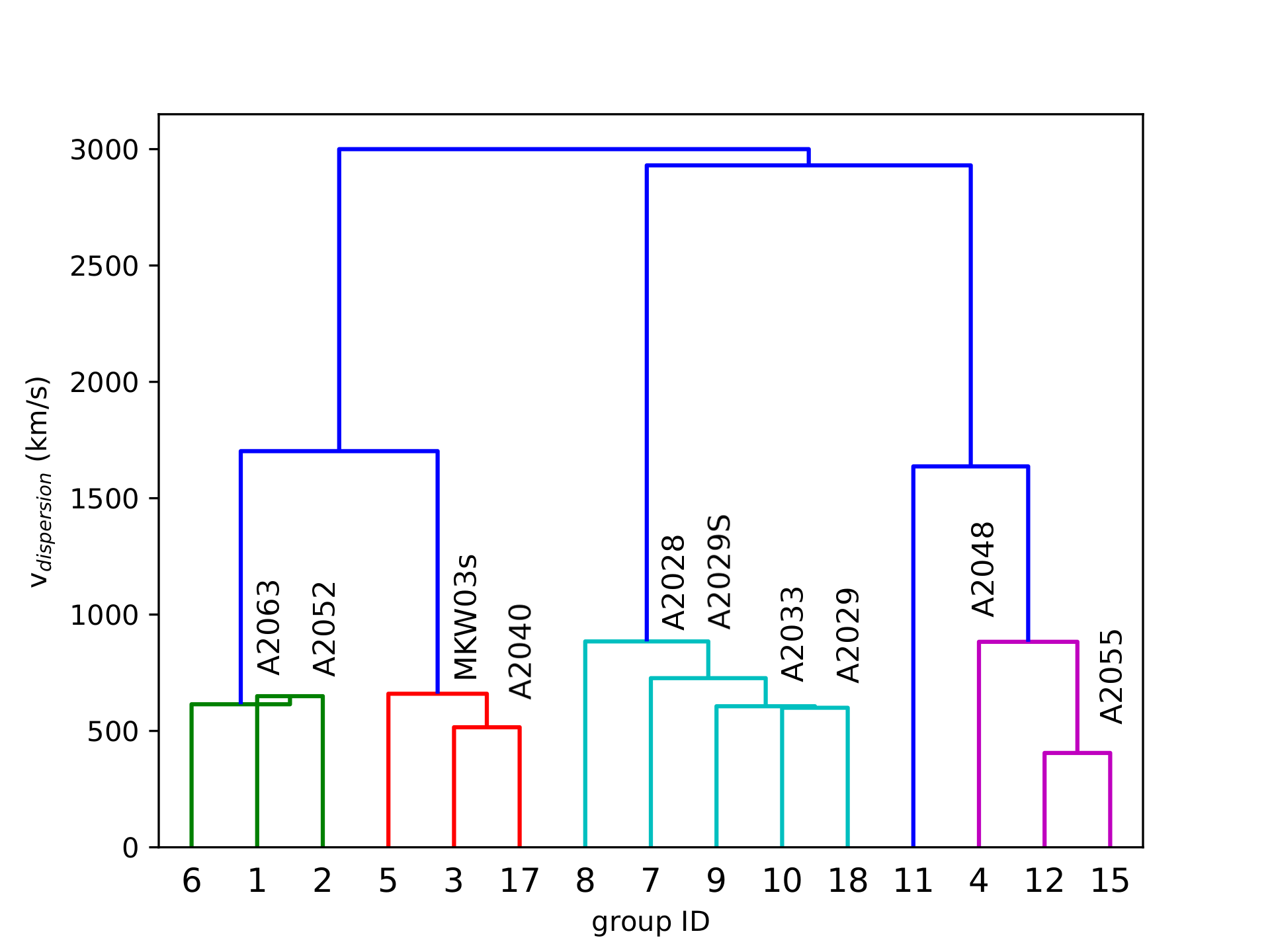
However, the approach of trimming the dendrogram according to the velocity dispersion plateau is mainly designed for individual galaxy clusters and is not suitable for large field-of-view multi-target studies. Fig.4 shows the spatial distribution of the simulated galaxy data and their corresponding dendrograms. Galaxy clusters with different masses have different velocity dispersion platforms and are hard to be extracted with a uniform threshold. Yu et al. (2018) proposed a new algorithm to trim the dendrogram—-“Blooming Tree”. Instead of setting a single threshold on the velocity dispersion, the new method traces all leaves and takes multiple properties —- the velocity dispersion, membership, and spatial distribution of each node into account to decide whether to trim the branch. The Blooming Tree algorithm is able to automatically detect all dense areas in the field without specifying their positions or redshifts. It significantly reduces the manual intervention in the analysis, improves the applicability of the method, and make the algorithm possible to analyze large-scale structures of the universe.
3.1.2 Supercluster
48 Superclusters are supermassive objects formed by the gravitational aggregation of multiple galaxy clusters. Because their scales are larger than 10 Mpc, the relaxation time exceeds the age of the universe. Therefore no distinct mass center or boundary has been formed. This poses a great difficulty for its definition and search. The methods of detecting superclusters usually derived from the algorithm of detecting galaxy clusters, the main methods are density of galaxy numbers(Einasto et al., 2007; Liivamägi et al., 2012), Friends-of-Firends algorithm(Luparello et al., 2011; Chon et al., 2013; Chow-Martínez et al., 2014; Liu et al., 2021), etc. However, our knowledge of such non-relaxation systems is still very limited because of the lack of effective evaluation methods.
Hierarchical clustering identifies galaxy clusters while also giving the hierarchy of their surroundings, and thus can provide new ideas for the detection of superclusters. We apply this algorithm (Blooming Tree) to the spectroscopic data of Sloan Digital Sky Survey (SDSS), and find many galaxy cluster candidates at different redshifts in the field of view of galaxy cluster A2029, as shown in Fig.5. The subordination between these structures can be seen directly in the simplified dendrogram on the bottom. Based on the typical velocity dispersion of the relaxation system at each level in the universe given by the virial theorem, we can roughly determine the position of the system at each level in the dendrogram. Velocity Dispersion 500km/s corresponding to galaxy groups, 1000km/s corresponding to galaxy clusters, the platform at 2000km/s indicates the presence of superclusters. Systems located in the same branch have strong gravitational associations with each other, while structures between different branches are more likely to have no direct gravitational connection. Furthermore, the order in which the systems merge into the branches can also tell how closely the members are related, so that the fiber structure can be found (We have detected in our analysis of galaxy cluster A85 an optical galaxy population corresponding to its outer X-ray fiber structure (Yu et al., 2016)), even the future merging sequence could be predicted. Santiago-Bautista et al. (2020) had also introduced hierarchical clustering algorithms to the detection of fiber structures in superclusters of galaxies.
3.1.3 Star Cluster
Stars may also assemble into clusters like galaxies. There are two types of star clusters: globular clusters and open clusters. The former are mostly located in galactic halos and have a regular spherical shape with a high density of member stars, and their origin is not clear; while the latter are born in molecular clouds and slowly disintegrate under many effects such as environmental perturbations, galactic tidal forces, and stellar evaporation, so their shape is very irregular. Star clusters are important objects for studying the evolution of stars and probing the structure of galaxies. The identification of cluster members is usually based on two a priori assumptions: one is the spatial position and motion information of the stars, assuming that cluster members have the same kinematic characteristics; the other is the magnitude and color information, assuming that member stars have the same evolutionary trends. Researchers have introduced various algorithms to identify cluster members based on these assumptions. Back in the middle of the last century, Vasilevskis et al. (1958) and Sanders (1971) had introduced the maximum likelihood method and double Gaussian fit to find the members of clusters. Many researchers have conducted numerous follow-up studies based on it (Zhao and He, 1990; Dias et al., 2006; Krone-Martins et al., 2010; Sarro et al., 2014; Sampedro and Alfaro, 2016), and this method is still the mainstream method in this field. In order to avoid the prior error introduced by Gaussian distribution, some researchers have introduced nonparametric methods to perform the fitting. However, these methods cannot get rid of the reliance on priori information. Recently, more modern clustering methods have been introduced into the field. Schmeja (2011) tested four clustering methods with two-dimensional projection data in 2011: star counts, nearest neighbour, Voronoi tessellation, minimum spanning tree(MST), etc, which was found to have the best combined performance for nearest-neighbor particles. Krone-Martins and Moitinho (2014) developed UPMASK method, combining with principal component analysis(PCA) and k-means algorithm, and applied for cluster analysis with the Gaia DR2 data. In addition, the effect of the DBSCAN algorithm was also tested by Gao (2014) and Castro-Ginard et al. (2018), respectively. The key parameters of these machine learning methods generally lack a reasonable physical interpretation, which has hindered the application and popularity of these methods.
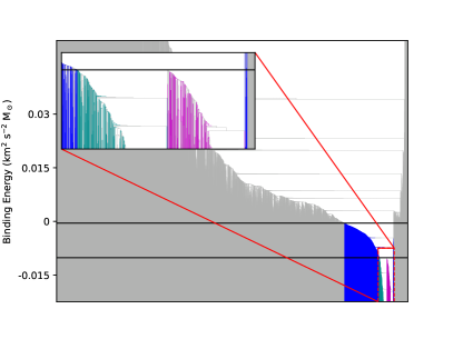
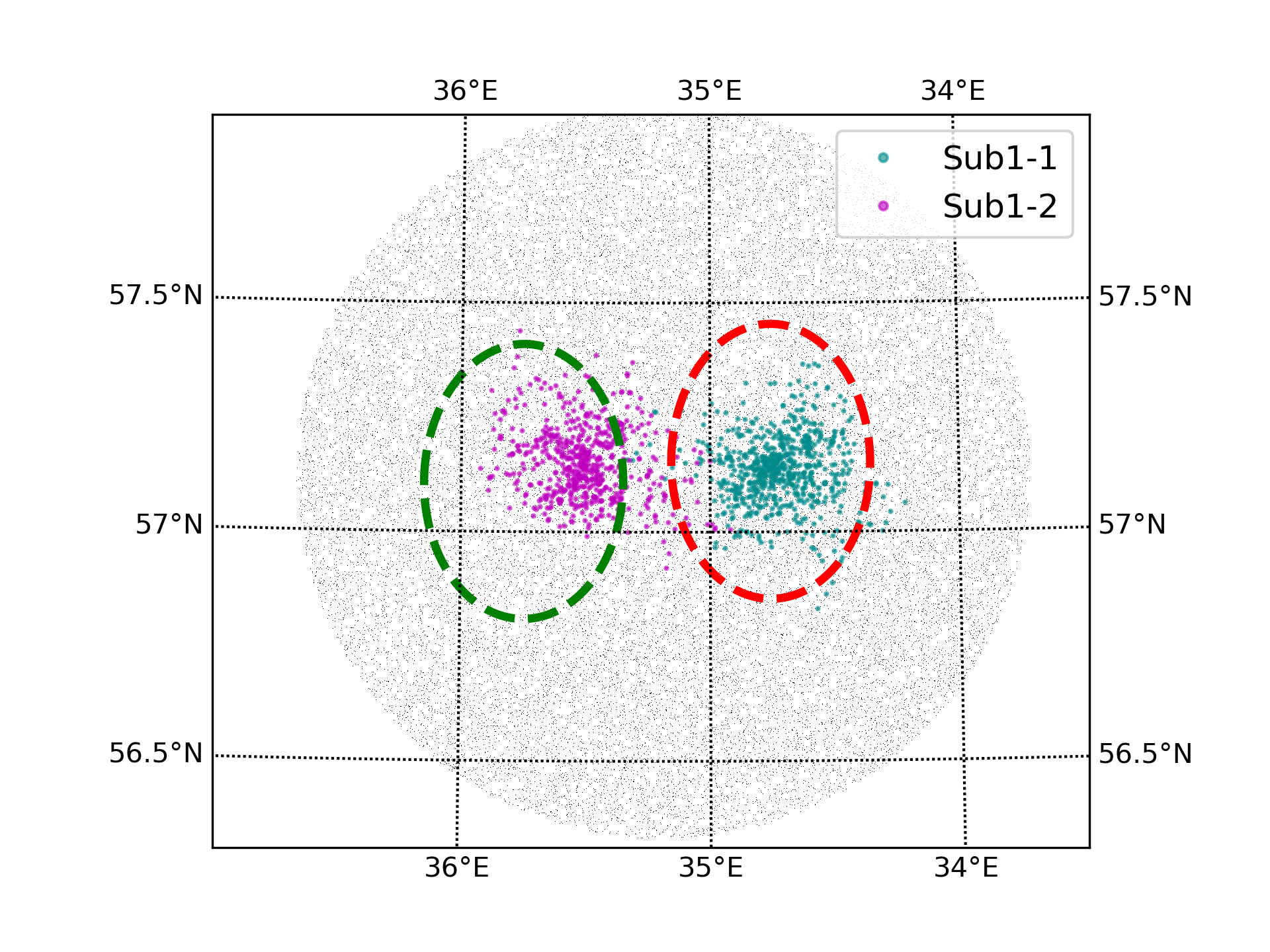
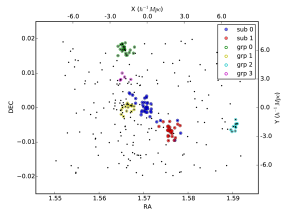
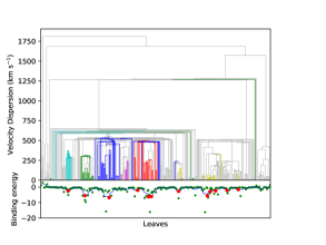
Hierarchical clustering methods do not require prior assumptions about the morphology or distribution of clusters. This is advantageous for exploring the boundaries of clusters and detecting clusters with low density or even disintegrating. Moreover, hierarchical clustering methods can not only give information about specific members, but also provide the hierarchical relationship of these members in the gravitational potential well. In fact, Rood (1983) had tried using hierarchical clustering algorithm to analyze nearby stars, but no clear conclusions were obtained. Yu et al. (2020) used Gaia DR2 data, tested the potential of hierarchical clustering algorithms for cluster structure analysis with the example of the open cluster Perseus Double Cluster. Perseus Double Cluster is a young cluster located at the distance of 2.34 kpc from the Sun, which contains two subclusters separated by about 46 arc minutes. It is not clear how the two subclusters overlap each other. Yu et al. (2020) selected the spatial position and proper motion in the field of view, with projection binding energy as a metric. The dendrogram obtained is shown in the Fig.6. The subsidence caused by the gravitational potential well of the cluster can be clearly seen in the dendrogram with the binding energy as the y-axis, and the stars deep in the potential well belong to two sub-clusters. According to the thresholds obtained from the velocity dispersion platform method, the halo members of the double cluster and the members of the two subclusters can be extracted from the field full of stars. The cluster members given by hierarchical clustering show a fairly good agreement in terms of color, parallax, etc. Compared with the traditional cluster member identification methods, the hierarchical clustering method only considers the kinematic information of the stars and does not depend on their physical properties such as luminosity or color. It provides a new way for the identification and study of cluster members.
3.1.4 Molecular Cloud
Although molecular clouds are not as discrete in distribution as stars or galaxies, they also have hierarchical features. Many studies have shown that high-density features in molecular clouds have relatively small physical scales and are always located in environments with low-density gas; for any scale, dense structures on small scales are more numerous than sparse structures on large scales (Rosolowsky et al., 2008). Dendrogram using hierarchical clustering algorithms can naturally identify such nested features and thus reflect the relationships between different types of structures in the data.
Houlahan and Scalo (1992) introduced the hierarchical clustering method to the study of the internal structure of molecular clouds for the first time. The dendrogram based on the molecular cloud column density and applied to the Taurus complex reveals a hierarchical structure in the star-forming molecular cloud complex. Rosolowsky et al. (2008) take each pixel point as a unit and use the position-position-velocity (PPV) data of that pixel point as a parameter in hierarchical clustering to calculate its correlation with surrounding pixel points. By quantifying the self-gravitating (self-gravitating) bound states of molecular clouds, they are able to distinguish between independent molecular clouds and substructures within molecular clouds. The new method was applied to the self-gravitational analysis and the identification of giant molecular clouds of Perseus L1448. It was compared with CLUMPFIND, the dominant algorithm for studying the structure of giant molecular clouds at that time. CLUMPFIND based on FoF algorithm, connects based on the values of the surrounding pixels and requires segmentation of the molecular cloud, focusing more on small-scale structures. Dendrogram, however, avoids segmentation and is able to cover large scale structures. Their results were later published in Nature letter (Goodman et al., 2009). Then, hierarchical clustering gained recognition in the field of molecular cloud research, and many subsequent studies were carried out based on it.
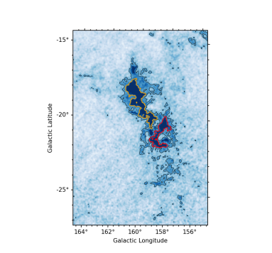
Colombo et al. (2015) designed the SCIMES algorithm based on the Rosolowsky et al. (2008) method, using PPV, 3D PPP data or 2D PP images as input data, and testing with data from the Orion-Chiron complex. They found characteristic volume and integrated CO luminosity can be used as valid criteria for trimming dendrograms to extract structure. And SCIMES performs better than CLUMPFIND in complex environments and high resolution data. Rice et al. (2016) used 12CO CfA-Chile survey data, dividing the galactic plane into four quadrants according to the size of the longitude, and then plotted dendrograms, respectively. Where the first quadrant () has a rich molecular cloud structure and a more complete research history, the dendrogram performs well in this complex environment, which is shown in Fig.7; and they obtained a catalog of 1064 giant molecular clouds in the entire galactic plane. Chen et al. (2020) applied the Rosolowsky et al. (2008) method to three-dimensional dust extinction and stellar color residual data to derive a distance catalog for giant molecular clouds at low latitudes, within 4 kpc of the Sun, with much higher distance accuracy than other methods. This is the first catalog of giant molecular clouds to derive distances in a direct way. Similarly, Guo et al. (2022) applies hierarchical clustering algorithm to the three-dimensional extinction map of the southern sky of the Milky Way, systematically verify and analyze the molecular clouds in there, and have obtained the first large-scale molecular cloud table of the southern sky with accurate distance measurement.
In addition to the usual PPV data, more multidimensional data can also be added for hierarchical clustering analysis. Henshaw et al. (2019) studied the internal dynamics of G0.253+0.016, one of the most massive and dense molecular clouds at the center of the galaxy. They added the centroid velocity and velocity dispersion to the spatial information, and found that the internal dynamical state is complex and has a hierarchical structure. Smullen et al. (2020) used magnetohydrodynamically simulated three-dimensional density fields to link the dendrogram structures through time, and by imposing constraints on the background cutoff, the minimum density increase for creating new structures, the minimum structure size, and the connection distance, they draw a physically consistent dendrogram and compare it with observations to study the time evolution of all dense cores in the region. In addition to the direct clustering of molecular clouds, the structure of molecular clouds can be studied indirectly by clustering of stars. Galli et al. (2019) used Gaia DR2 data to cluster the newly born stars in the Taurus complex, linking the stellar positions and physical parameters to the molecular clouds in which they are located. They grouped the molecular clouds corresponding to these stars in space into 21 subgroups, revealing the coupling between stars and molecular clouds in velocity and space.
From these works, it can be seen that the hierarchical clustering method has become increasingly widespread and diverse in the application of molecular cloud research.
3.2 Classification of Celestial Bodies
The classification of celestial bodies is a fundamental part of astronomical research. Traditionally, the classification of celestial bodies is done manually by astronomers based on experience. As astronomy technology advances, astronomical data sets become larger and larger. To analyze these data effectively, discover previously unknown objects and features, and search for potential associations and patterns are new challenges posed by big data. The unsupervised hierarchical clustering method is particularly well suited to handle the need for automatic classification without a priori information. The hierarchical results it gives also provide valuable clues for the subsequent parameter tuning. Therefore there are many astronomical classification studies that have applied the hierarchical clustering method.
Eigenson and Yatsyk (1987) had tried applying hierarchical clustering algorithm to automatically classify globular and open clusters based on information such as luminosity, scale, color index, and metal abundance. This work has not received enough attention, though.
Zappala et al. (1990, 1994) used this method to classify asteroid according to three-dimensional proper element. In 1995, they compared the results of this method with those of wavelet analysis using a sample containing 12,487 asteroids data, and found that the two methods gave essentially the same classification results for the major asteroid families (Zappalà et al., 1995). Carruba and Michtchenko (2007) referred to this method proposed that to hierarchical clustering by using proper frequency, which also identified asteroid families successfully. After optimized the distance metric, it even can recognize tynamical evolution of asteroid families (Carruba and Michtchenko, 2009). They analyzed multiple asteroid families with this method (Carruba et al., 2015, 2016). With the rapid increase in the number of asteroids, Milani et al. (2014) also used the hierarchical clustering to classify asteroid families, and even identify the collision fragments in them (Milani et al., 2019). A relevant review in this direction can be found in the paper published by Knežević (2016).
Raw images or spectral data of celestial objects are usually not directly usable for drawing dendrograms and need to be quantified with the help of suitable methods. Hojnacki et al. (2007) attempted an automated classification study of X-ray astronomical spectra. They first extracted the main information in the spectra by principal component analysis (PCA), then grouped them by the hierarchical clustering, and finally determined the members of each group by the k-means method. In the same period, Marchi (2007) also used a similar idea to classify exoplanets. They first used PCA to identify key variables and then used these new variables to perform hierarchical clustering to obtain exoplanet classification. Marchi et al. (2009) also used this method to discuss the origin of exoplanets. Peth et al. (2016) used hierarchical clustering to process the results of PCA analysis of high-redshift optical galaxies to morphologically classify them in order to avoid the subjective errors introduced by manual classification. Hocking et al. (2018) also proposed a similar idea to identify galaxy morphology. They first tried to quantify the spatial morphology of galaxies, and then clustered the quantified results using the hierarchical clustering. Their classification results are generally consistent compared to the manual annotation results from the Galaxy Zoo (Hocking et al., 2018).
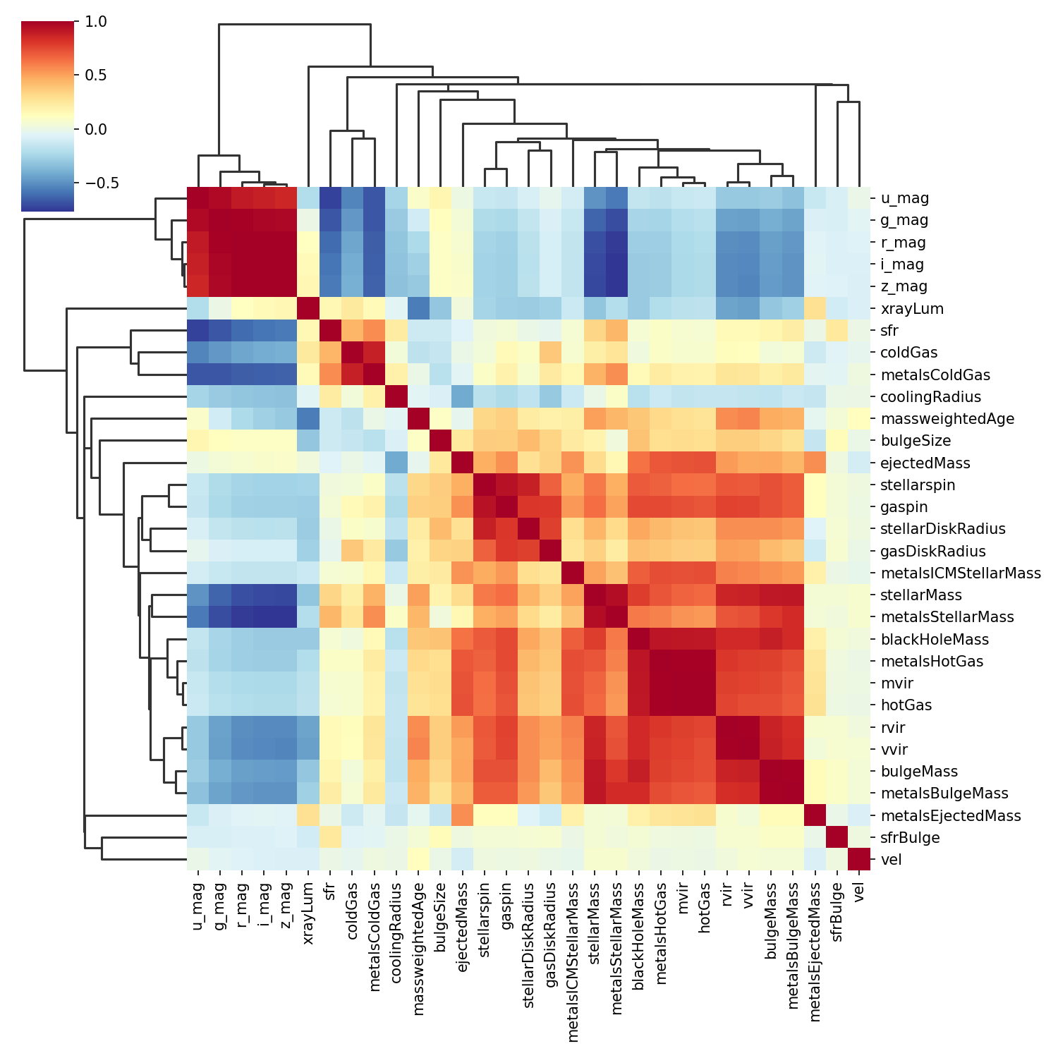
Hierarchical clustering is often used in combination with correlation matrix or heat map, to reveal the correlation between multivariate variables. The early development of this method has been discussed detailed in the review of Wilkinson and Friendly (2009). The popular statistical analysis language R and the popular programming language Python both have ready-made functions to plot heat maps. de Souza and Ciardi (2015) develops AMANDA in R to progress multidimensional astronomy data, which is able to hierarchical cluster correlation matrix. They test with simulated galaxy data, and Fig. 8 shows that ugriz- band brightness in galaxies are highly correlated. The first use of this technique in the field of astronomy may be Baron et al. (2015). In their analysis of diffuse interstellar absorption bands (DIBs) of unknown origin, they used the hierarchical clustering method to process the correlation matrix between 142 DIB spectral lines to find potential families of spectral lines among them. They found that the spectral line families given by hierarchical clustering can be interpreted as absorption lines from the same molecule.
Hierarchical clustering has even been used for classification of time-varying data. Ma et al. (2018) tested this method in the type identification of coronal mass ejections (CMEs). However, they found that it was not as effective as the previous method, distance density clustering (DDC).
Overall, the hierarchical clustering algorithm is still in the early stages of experimentation in the field of celestial body classification except for asteroid identification. Although it has attracted the attention of many researchers in different astronomical fields, the procedure and the performance is different from case to case. To use it as a reliable automatic classification tool, a lot of tuning work is neccessary.
4 Conclusion
As a mature data analysis method, hierarchical clustering has attracted the attention of researchers in many branches of astronomy, and achieved a certain extent of recognition. But it’s not a grab-and-go tool, it needs targeted design based on he actual data characteristics and scientific objectives.
The dendrogram obtained by hierarchical clustering is particularly suitable for describing hierarchical structure of gravitational systems. So it has a wide range of applications in gravitational systems at all levels of the universe like molecular clouds, star clusters, galaxy clusters and superclusters. In addition to identifying the members of these systems, its unique advantages are reflecting the dynamical state and evolutionary trend of members. As long as researchers handle the explanation and stability of the hierarchical clustering, it will play a bigger role in these fields.
In celestial body identification and classification, the unsupervised automated classification represented by the hierarchical clustering algorithm is expected to help astronomers search for unknown types of celestial objects and astronomical events. However, we also note that the form of implementation and the way of the hierarchical clustering algorithm work in different domains varies greatly due to the different knowledge structures and backgrounds of researchers. Although these papers use the same core algorithm, there are many differences in their algorithmic formulations, working logic, analytical tools, and even terminology names. If these can learn from each other, it will undoubtedly help us to make full use of the algorithm.
Of course, there are still some limitations of the hierarchical clustering algorithm. The key one is the computational complexity. The computation and storage of the two-by-two distance matrix between sets is an essential step for the hierarchical clustering. This determines the complexity of the hierarchical clustering algorithm to be at least , and it’s difficult to handle data sets of more than 100,000 records now. And the same type of FoF algorithm only needs to use a specific trim threshold as a criterion to reduce the distance matrix to a Boolean matrix and retain only the grouping information, thus reducing the computational difficulty and storage cost. Its complexity is . Therefore, to apply the hierarchical clustering algorithm to large astronomical data sets, further optimization is needed to reduce its computational cost.
With the construction of a new generation of astronomical equipment, modern astronomy is entering an era of all-sky, all-wavelength, all-time observations, and the amount of data to be analyzed is exploding. New tools need to be developed and evolved to make truly valuable scientific discoveries with limited staff and computing power.
References
- Adami et al. (2005) Adami, C., Biviano, A., Durret, F., Mazure, A., 2005. The build-up of the Coma cluster by infalling substructures. Astronomy and Astrophysics 443, 17–27. doi:10.1051/0004-6361:20053504, arXiv:astro-ph/0507542.
- Babu and Feigelson (1996) Babu, G.J., Feigelson, E.D., 1996. Astrostatistics. CRC Press, Boca Raton, Florida.
- Baron (2019) Baron, D., 2019. Machine Learning in Astronomy: a practical overview. arXiv e-prints , arXiv:1904.07248arXiv:1904.07248.
- Baron et al. (2015) Baron, D., Poznanski, D., Watson, D., Yao, Y., Cox, N.L.J., Prochaska, J.X., 2015. Using Machine Learning to classify the diffuse interstellar bands. Monthly Notices of the Royal Astronomy Society 451, 332--352. doi:10.1093/mnras/stv977, arXiv:1501.04631.
- Carruba et al. (2016) Carruba, V., Aljbaae, S., Winter, O.C., 2016. On the Erigone family and the z2 secular resonance. Monthly Notices of the Royal Astronomy Society 455, 2279--2288. doi:10.1093/mnras/stv2430, arXiv:1510.05551.
- Carruba and Michtchenko (2007) Carruba, V., Michtchenko, T.A., 2007. A frequency approach to identifying asteroid families. Astronomy and Astrophysics 475, 1145--1158. doi:10.1051/0004-6361:20077689.
- Carruba and Michtchenko (2009) Carruba, V., Michtchenko, T.A., 2009. A frequency approach to identifying asteroid families. II. Families interacting with nonlinear secular resonances and low-order mean-motion resonances. Astronomy and Astrophysics 493, 267--282. doi:10.1051/0004-6361:200809852.
- Carruba et al. (2015) Carruba, V., Nesvorný, D., Aljbaae, S., Huaman, M.E., 2015. Dynamical evolution of the Cybele asteroids. Monthly Notices of the Royal Astronomy Society 451, 244--256. doi:10.1093/mnras/stv997, arXiv:1505.03745.
- Castro-Ginard et al. (2018) Castro-Ginard, A., Jordi, C., Luri, X., Julbe, F., Morvan, M., Balaguer-Núñez, L., Cantat-Gaudin, T., 2018. A new method for unveiling open clusters in Gaia. New nearby open clusters confirmed by DR2. Astronomy and Astrophysics 618, A59. doi:10.1051/0004-6361/201833390, arXiv:1805.03045.
- Chen et al. (2020) Chen, B.Q., Li, G.X., Yuan, H.B., Huang, Y., Tian, Z.J., Wang, H.F., Zhang, H.W., Wang, C., Liu, X.W., 2020. A large catalogue of molecular clouds with accurate distances within 4 kpc of the Galactic disc. Monthly Notices of the Royal Astronomy Society 493, 351--361. doi:10.1093/mnras/staa235, arXiv:2001.11682.
- Chon et al. (2013) Chon, G., Böhringer, H., Nowak, N., 2013. The extended ROSAT-ESO Flux-Limited X-ray Galaxy Cluster Survey (REFLEX II) - III. Construction of the first flux-limited supercluster sample. Monthly Notices of the Royal Astronomy Society 429, 3272--3287. doi:10.1093/mnras/sts584, arXiv:1212.1597.
- Chow-Martínez et al. (2014) Chow-Martínez, M., Andernach, H., Caretta, C.A., Trejo-Alonso, J.J., 2014. Two new catalogues of superclusters of Abell/ACO galaxy clusters out to redshift 0.15. Monthly Notices of the Royal Astronomy Society 445, 4073--4085. doi:10.1093/mnras/stu1961, arXiv:1409.5152.
- Colombo et al. (2015) Colombo, D., Rosolowsky, E., Ginsburg, A., Duarte-Cabral, A., Hughes, A., 2015. Graph-based interpretation of the molecular interstellar medium segmentation. Monthly Notices of the Royal Astronomy Society 454, 2067--2091. doi:10.1093/mnras/stv2063, arXiv:1510.04253.
- de Souza and Ciardi (2015) de Souza, R.S., Ciardi, B., 2015. AMADA-Analysis of multidimensional astronomical datasets. Astronomy and Computing 12, 100--108. doi:10.1016/j.ascom.2015.06.006, arXiv:1503.07736.
- Defays (1977) Defays, D., 1977. An efficient algorithm for a complete link method. The Computer Journal 20, 364--366.
- Diaferio (1999) Diaferio, A., 1999. Mass estimation in the outer regions of galaxy clusters. Monthly Notices of the Royal Astronomical Society 309, 610--622. URL: http://adsabs.harvard.edu/abs/1999MNRAS.309..610D.
- Dias et al. (2006) Dias, W.S., Assafin, M., Flório, V., Alessi, B.S., Líbero, V., 2006. Proper motion determination of open clusters based on the UCAC2 catalogue. Astronomy and Astrophysics 446, 949--953. doi:10.1051/0004-6361:20052741.
- Eigenson and Yatsyk (1987) Eigenson, A.M., Yatsyk, O.S., 1987. Star Cluster Taxonomy. Soviet Astronomy Letters 13, 197.
- Einasto et al. (2007) Einasto, J., Einasto, M., Tago, E., Saar, E., Hütsi, G., Jõeveer, M., Liivamägi, L.J., Suhhonenko, I., Jaaniste, J., Heinämäki, P., Müller, V., Knebe, A., Tucker, D., 2007. Superclusters of galaxies from the 2dF redshift survey. I. The catalogue. Astronomy and Astrophysics 462, 811--825. doi:10.1051/0004-6361:20065296, arXiv:astro-ph/0603764.
- Everitt et al. (2011) Everitt, B.S., Landau, S., Leese, M., Stahl, D., 2011. Cluster Analysis, 5th Edition. Wiley Online Library, Hoboken, NJ.
- Galli et al. (2019) Galli, P.A.B., Loinard, L., Bouy, H., Sarro, L.M., Ortiz-León, G.N., Dzib, S.A., Olivares, J., Heyer, M., Hernandez, J., Román-Zúñiga, C., Kounkel, M., Covey, K., 2019. Structure and kinematics of the Taurus star-forming region from Gaia-DR2 and VLBI astrometry. Astronomy and Astrophysics 630, A137. doi:10.1051/0004-6361/201935928, arXiv:1909.01118.
- Gao (2014) Gao, X.H., 2014. Membership determination of open cluster NGC 188 based on the DBSCAN clustering algorithm. Research in Astronomy and Astrophysics 14, 159--164. doi:10.1088/1674-4527/14/2/004.
- Garcia (1993) Garcia, A.M., 1993. General study of group membership. II. Determination of nearby groups. Astronomy and Astrophysicss 100, 47--90.
- Garcia et al. (1992) Garcia, A.M., Morenas, V., Paturel, G., 1992. A search for a quantitative comparison of galaxy clustering algorithms. Astronomy and Astrophysics 253, 74--76.
- Goodman et al. (2009) Goodman, A.A., Rosolowsky, E.W., Borkin, M.A., Foster, J.B., Halle, M., Kauffmann, J., Pineda, J.E., 2009. A role for self-gravity at multiple length scales in the process of star formation. Nature 457, 63--66. doi:10.1038/nature07609.
- Gordon (1987) Gordon, A.D., 1987. A review of hierarchical classification. Journal of the Royal Statistical Society: Series A (General) 150, 119--137. URL: https://rss.onlinelibrary.wiley.com/doi/abs/10.2307/2981629, doi:https://doi.org/10.2307/2981629, arXiv:https://rss.onlinelibrary.wiley.com/doi/pdf/10.2307/2981629.
- Gourgoulhon et al. (1992) Gourgoulhon, E., Chamaraux, P., Fouque, P., 1992. Groups of galaxies within 80 Mpc. I - Grouping hierarchical method and statistical properties. Astronomy and Astrophysics 255, 69--86.
- Guennou et al. (2014) Guennou, L., Adami, C., Durret, F., Lima Neto, G.B., Ulmer, M.P., Clowe, D., LeBrun, V., Martinet, N., Allam, S., Annis, J., Basa, S., Benoist, C., Biviano, A., Cappi, A., Cypriano, E.S., Gavazzi, R., Halliday, C., Ilbert, O., Jullo, E., Just, D., Limousin, M., Márquez, I., Mazure, A., Murphy, K.J., Plana, H., Rostagni, F., Russeil, D., Schirmer, M., Slezak, E., Tucker, D., Zaritsky, D., Ziegler, B., 2014. Structure and substructure analysis of DAFT/FADA galaxy clusters in the [0.4-0.9] redshift range. Astronomy and Astrophysics 561, A112. doi:10.1051/0004-6361/201321208, arXiv:1311.6922.
- Guo et al. (2022) Guo, H.L., Chen, B.Q., Liu, X.W., 2022. A large catalogue of molecular clouds in the Southern sky. Monthly Notices of the Royal Astronomy Society 511, 2302--2312. doi:10.1093/mnras/stac213, arXiv:2201.09578.
- Henshaw et al. (2019) Henshaw, J.D., Ginsburg, A., Haworth, T.J., Longmore, S.N., Kruijssen, J.M.D., Mills, E.A.C., Sokolov, V., Walker, D.L., Barnes, A.T., Contreras, Y., Bally, J., Battersby, C., Beuther, H., Butterfield, N., Dale, J.E., Henning, T., Jackson, J.M., Kauffmann, J., Pillai, T., Ragan, S., Riener, M., Zhang, Q., 2019. ‘The Brick’ is not a brick: a comprehensive study of the structure and dynamics of the central molecular zone cloud G0.253+0.016. Monthly Notices of the Royal Astronomy Society 485, 2457--2485. doi:10.1093/mnras/stz471, arXiv:1902.02793.
- Hocking et al. (2018) Hocking, A., Geach, J.E., Sun, Y., Davey, N., 2018. An automatic taxonomy of galaxy morphology using unsupervised machine learning. Monthly Notices of the Royal Astronomy Society 473, 1108--1129. doi:10.1093/mnras/stx2351, arXiv:1709.05834.
- Hojnacki et al. (2007) Hojnacki, S.M., Kastner, J.H., Micela, G., Feigelson, E.D., LaLonde, S.M., 2007. An X-Ray Spectral Classification Algorithm with Application to Young Stellar Clusters. Astrophysics Journal 659, 585--598. doi:10.1086/512232.
- Houlahan and Scalo (1992) Houlahan, P., Scalo, J., 1992. Recognition and Characterization of Hierarchical Interstellar Structure. II. Structure Tree Statistics. Astrophysics Journal 393, 172. doi:10.1086/171495.
- Hsu et al. (2013) Hsu, L.Y., Ebeling, H., Richard, J., 2013. The three-dimensional geometry and merger history of the massive galaxy cluster MACS J0358.8-2955. Monthly Notices of the Royal Astronomy Society 429, 833--848. doi:10.1093/mnras/sts379, arXiv:1209.2492.
- Huchra and Geller (1982) Huchra, J.P., Geller, M.J., 1982. Groups of Galaxies. I. Nearby groups. Astrophysics Journal 257, 423--437. doi:10.1086/160000.
- Ivezić et al. (2014) Ivezić, Ž., Connolly, A.J., VanderPlas, J.T., Gray, A., 2014. Statistics, Data Mining, and Machine Learning in Astronomy: A Practical Python Guide for the Analysis of Survey Data. Princeton University Press, Princeton, NJ. doi:10.1515/9781400848911.
- Knežević (2016) Knežević, Z., 2016. Asteroid Family Identification: History and State of the Art, in: Chesley, S.R., Morbidelli, A., Jedicke, R., Farnocchia, D. (Eds.), Asteroids: New Observations, New Models, pp. 16--27. doi:10.1017/S1743921315008728.
- Krone-Martins and Moitinho (2014) Krone-Martins, A., Moitinho, A., 2014. UPMASK: unsupervised photometric membership assignment in stellar clusters. Astronomy and Astrophysics 561, A57. doi:10.1051/0004-6361/201321143, arXiv:1309.4471.
- Krone-Martins et al. (2010) Krone-Martins, A., Soubiran, C., Ducourant, C., Teixeira, R., Le Campion, J.F., 2010. Kinematic parameters and membership probabilities of open clusters in the Bordeaux PM2000 catalogue. Astronomy and Astrophysics 516, A3. doi:10.1051/0004-6361/200913881, arXiv:1006.0096.
- Lance and Williams (1967) Lance, G.N., Williams, W.T., 1967. A General Theory of Classificatory Sorting Strategies: 1. Hierarchical Systems. The Computer Journal 9, 373--380. URL: https://doi.org/10.1093/comjnl/9.4.373, doi:10.1093/comjnl/9.4.373, arXiv:https://academic.oup.com/comjnl/article-pdf/9/4/373/1101470/9-4-373.pdf.
- Liivamägi et al. (2012) Liivamägi, L.J., Tempel, E., Saar, E., 2012. SDSS DR7 superclusters. The catalogues. Astronomy and Astrophysics 539, A80. doi:10.1051/0004-6361/201016288, arXiv:1012.1989.
- Liu et al. (2021) Liu, A., Bulbul, E., Ghirardini, V., Liu, T., Klein, M., Clerc, N., Oezsoy, Y., Ramos-Ceja, M.E., Pacaud, F., Comparat, J., Okabe, N., Bahar, Y.E., Biffi, V., Brunner, H., Brueggen, M., Buchner, J., Ider Chitham, J., Chiu, I., Dolag, K., Gatuzz, E., Gonzalez, J., Hoang, D.N., Lamer, G., Merloni, A., Nandra, K., Oguri, M., Ota, N., Predehl, P., Reiprich, T.H., Salvato, M., Schrabback, T., Sanders, J.S., Seppi, R., Thibaud, Q., 2021. The eROSITA Final Equatorial-Depth Survey (eFEDS): Catalog of galaxy clusters and groups. arXiv e-prints , arXiv:2106.14518arXiv:2106.14518.
- Liu et al. (2018) Liu, A., Yu, H., Diaferio, A., Tozzi, P., Hwang, H.S., Umetsu, K., Okabe, N., Yang, L.L., 2018. Inside a Beehive: The Multiple Merging Processes in the Galaxy Cluster Abell 2142. Astrophysics Journal 863, 102. doi:10.3847/1538-4357/aad090, arXiv:1806.10864.
- Luparello et al. (2011) Luparello, H., Lares, M., Lambas, D.G., Padilla, N., 2011. Future virialized structures: an analysis of superstructures in the SDSS-DR7. Monthly Notices of the Royal Astronomy Society 415, 964--976. doi:10.1111/j.1365-2966.2011.18794.x, arXiv:1101.1961.
- Ma et al. (2018) Ma, R., Angryk, R.A., Riley, P., Filali Boubrahimi, S., 2018. Coronal Mass Ejection Data Clustering and Visualization of Decision Trees. Astrophysics Journals 236, 14. doi:10.3847/1538-4365/aab76f.
- Marchi (2007) Marchi, S., 2007. Extrasolar Planet Taxonomy: A New Statistical Approach. Astrophysics Journal 666, 475--485. doi:10.1086/519760, arXiv:0705.0910.
- Marchi et al. (2009) Marchi, S., Ortolani, S., Nagasawa, M., Ida, S., 2009. On the various origins of close-in extrasolar planets. Monthly Notices of the Royal Astronomy Society 394, L93--L96. doi:10.1111/j.1745-3933.2009.00619.x, arXiv:0901.1547.
- Materne (1978) Materne, J., 1978. The structure of nearby clusters of galaxies. Hierarchical clustering and an application to the Leo region. Astronomy and Astrophysics 63, 401--409.
- Milani et al. (2014) Milani, A., Cellino, A., Knežević, Z., Novaković, B., Spoto, F., Paolicchi, P., 2014. Asteroid families classification: Exploiting very large datasets. Icarus 239, 46--73. doi:10.1016/j.icarus.2014.05.039, arXiv:1312.7702.
- Milani et al. (2019) Milani, A., Knežević, Z., Spoto, F., Paolicchi, P., 2019. Asteroid cratering families: recognition and collisional interpretation. Astronomy and Astrophysics 622, A47. doi:10.1051/0004-6361/201834056, arXiv:1812.07535.
- Peth et al. (2016) Peth, M.A., Lotz, J.M., Freeman, P.E., McPartland, C., Mortazavi, S.A., Snyder, G.F., Barro, G., Grogin, N.A., Guo, Y., Hemmati, S., Kartaltepe, J.S., Kocevski, D.D., Koekemoer, A.M., McIntosh, D.H., Nayyeri, H., Papovich, C., Primack, J.R., Simons, R.C., 2016. Beyond spheroids and discs: classifications of CANDELS galaxy structure at 1.4 < z < 2 via principal component analysis. Monthly Notices of the Royal Astronomy Society 458, 963--987. doi:10.1093/mnras/stw252, arXiv:1504.01751.
- Rice et al. (2016) Rice, T.S., Goodman, A.A., Bergin, E.A., Beaumont, C., Dame, T.M., 2016. A Uniform Catalog of Molecular Clouds in the Milky Way. Astrophysics Journal 822, 52. doi:10.3847/0004-637X/822/1/52, arXiv:1602.02791.
- Rood (1983) Rood, H.J., 1983. Dendogram Cosmography - the Stars Within 25 Parsecs, in: Philip, A.G.D., Upgren, A.R. (Eds.), IAU Colloq. 76: Nearby Stars and the Stellar Luminosity Function, p. 411.
- Rosolowsky et al. (2008) Rosolowsky, E.W., Pineda, J.E., Kauffmann, J., Goodman, A.A., 2008. Structural Analysis of Molecular Clouds: Dendrograms. Astrophysics Journal 679, 1338--1351. doi:10.1086/587685, arXiv:0802.2944.
- Sampedro and Alfaro (2016) Sampedro, L., Alfaro, E.J., 2016. Stellar open clusters’ membership probabilities: an N-dimensional geometrical approach. Monthly Notices of the Royal Astronomy Society 457, 3949--3962. doi:10.1093/mnras/stw243, arXiv:1602.01025.
- Sanders (1971) Sanders, W.L., 1971. An improved method for computing membership probabilities in open clusters. Astronomy and Astrophysics 14, 226--232.
- Santiago-Bautista et al. (2020) Santiago-Bautista, I., Caretta, C.A., Bravo-Alfaro, H., Pointecouteau, E., Andernach, H., 2020. Identification of filamentary structures in the environment of superclusters of galaxies in the Local Universe. Astronomy and Astrophysics 637, A31. doi:10.1051/0004-6361/201936397, arXiv:2002.03446.
- Sarro et al. (2014) Sarro, L.M., Bouy, H., Berihuete, A., Bertin, E., Moraux, E., Bouvier, J., Cuillandre, J.C., Barrado, D., Solano, E., 2014. Cluster membership probabilities from proper motions and multi-wavelength photometric catalogues. I. Method and application to the Pleiades cluster. Astronomy and Astrophysics 563, A45. doi:10.1051/0004-6361/201322413, arXiv:1401.7427.
- Schmeja (2011) Schmeja, S., 2011. Identifying star clusters in a field: A comparison of different algorithms. Astronomische Nachrichten 332, 172. doi:10.1002/asna.201011484, arXiv:1011.5533.
- Serna and Gerbal (1996) Serna, A., Gerbal, D., 1996. Dynamical search for substructures in galaxy clusters. A hierarchical clustering method. Astronomy and Astrophysics 309, 65--74. arXiv:astro-ph/9509080.
- Serra and Diaferio (2013) Serra, A.L., Diaferio, A., 2013. Identification of Members in the Central and Outer Regions of Galaxy Clusters. Astrophysics Journal 768, 116. doi:10.1088/0004-637X/768/2/116, arXiv:1211.3669.
- Sibson (1973) Sibson, R., 1973. Slink: An optimally efficient algorithm for the single-link cluster method. Computer Journal 16, 30--34.
- Smullen et al. (2020) Smullen, R.A., Kratter, K.M., Offner, S.S.R., Lee, A.T., Chen, H.H.H., 2020. The highly variable time evolution of star-forming cores identified with dendrograms. Monthly Notices of the Royal Astronomy Society 497, 4517--4534. doi:10.1093/mnras/staa2253, arXiv:2004.01263.
- Sørensen (1948) Sørensen, T., 1948. A method of establishing group of equal amplitude in plant sociobiology based on similarity of species content and its application to analyses of the vegetation on danish commons, in: Biologiske Skrifter.
- Tully (1980) Tully, R.B., 1980. Nearby groups of galaxies. I - The NGC 1023 group. The Astrophysical Journal 237, 390--403. URL: http://adsabs.harvard.edu/abs/1980ApJ...237..390T, doi:10.1086/157881.
- Tully (1987) Tully, R.B., 1987. Nearby groups of galaxies. II - an all-sky survey within 3000 kilometers per second. The Astrophysical Journal 321, 280--304. URL: http://adsabs.harvard.edu/abs/1987ApJ...321..280T, doi:10.1086/165629.
- Vasilevskis et al. (1958) Vasilevskis, S., Klemola, A., Preston, G., 1958. Relative proper motions of stars in the region of the open cluster NGC 6633. Astronomical Journal 63, 387--395. doi:10.1086/107787.
- WANG and YU (2021) WANG, L., YU, H., 2021. On merging galaxy cluster macs j0358.8-2955. Beijing Normal University(Natural Science) 57, 186--193.
- Wilkinson and Friendly (2009) Wilkinson, L., Friendly, M., 2009. The history of the cluster heat map. The American Statistician 63, 179--184.
- Yu et al. (2016) Yu, H., Diaferio, A., Agulli, I., Aguerri, J.A.L., Tozzi, P., 2016. The unrelaxed dynamical structure of the galaxy cluster abell 85. The Astrophysical Journal 831. URL: http://adsabs.harvard.edu/abs/2016ApJ...831..156Y.
- Yu et al. (2018) Yu, H., Diaferio, A., Serra, A.L., Baldi, M., 2018. Blooming Trees: Substructures and Surrounding Groups of Galaxy Clusters. Astrophysics Journal 860, 118. doi:10.3847/1538-4357/aac263, arXiv:1805.12306.
- Yu et al. (2015) Yu, H., Serra, A.L., Diaferio, A., Baldi, M., 2015. Identification of Galaxy Cluster Substructures with the Caustic Method. Astrophysics Journal 810, 37. doi:10.1088/0004-637X/810/1/37, arXiv:1503.08823.
- Yu et al. (2020) Yu, H., Shao, Z., Diaferio, A., Li, L., 2020. Unveiling the Hierarchical Structure of Open Star Clusters: The Perseus Double Cluster. Astrophysics Journal 899, 144. doi:10.3847/1538-4357/aba8f3, arXiv:2007.11850.
- Zappalà et al. (1995) Zappalà, V., Bendjoya, P., Cellino, A., Farinella, P., Froeschlé, C., 1995. Asteroid families: Search of a 12,487-asteroid sample using two different clustering techniques. Icarus 116, 291--314. doi:10.1006/icar.1995.1127.
- Zappala et al. (1990) Zappala, V., Cellino, A., Farinella, P., Knezevic, Z., 1990. Asteroid Families. I. Identification by Hierarchical Clustering and Reliability Assessment. Astronomical Journal 100, 2030. doi:10.1086/115658.
- Zappala et al. (1994) Zappala, V., Cellino, A., Farinella, P., Milani, A., 1994. Asteroid Famalies. II. Extension to Unnumbered Multiopposition Asteroids. Astronomical Journal 107, 772. doi:10.1086/116897.
- Zhao and He (1990) Zhao, J.L., He, Y.P., 1990. An improved method for membership determination of stellar clusters with proper motions with different accuracies. Astronomy and Astrophysics 237, 54.