Data-Driven Disease Progression Modelling

Abstract

Intense debate in the Neurology community before 2010 culminated in hypothetical models of Alzheimer’s disease progression: a pathophysiological cascade of biomarkers, each dynamic for only a segment of the full disease timeline. Inspired by this, data-driven disease progression modelling emerged from the computer science community with the aim to reconstruct neurodegenerative disease timelines using data from large cohorts of patients, healthy controls, and prodromal/at-risk individuals. This chapter describes selected highlights from the field, with a focus on utility for understanding and forecasting of disease progression.

1. Introduction

Chronic progressive diseases are a major drain on social and economic resources. Many of these diseases have no treatments and no cure. In particular, age-related chronic diseases such as neurodegenerative diseases of the brain are a global healthcare pandemic-in-waiting as most of the world’s population is living ever longer. A key example is Alzheimer’s disease — the leading cause of dementia — but there are numerous other conditions that cause abnormal deterioration of brain tissue, leading to loss of cognitive performance, bodily function, independence, and ultimately death. Despite the increasing socioeconomic burden, neurodegenerative disease research has made impressive progress in the past decade, driven largely by the availability of large observational datasets and the computational analyses this enables.

Understanding neurodegenerative diseases is vital if they are to be managed, or even cured, but our understanding remains poor despite impressive progress in recent years. This poor understanding can be attributed to the many challenges of neurodegenerative diseases: no well-defined time axis due in part to heterogeneity in onset/speed/presentation, and censoring/attrition especially in later stages as patients deteriorate. These challenges, coupled with intense debate in the Neurology community (hypothetical models [1, 2]) and increasing availability of data, piqued the interest of computational researchers aiming to provide quantitative answers to the mysteries of neurodegenerative diseases. This has ranged from vanilla off-the-shelf machine learning approaches through to more holistic statistical modelling approaches, the most advanced of which is data-driven disease progression modelling (D³PM).

D³PMs are defined by two key features: 1) they simultaneously reconstruct the disease timeline and estimate the quantitative disease signature/trajectory along this timeline; and 2) they are directly informed by observed data. D³PMs strike a balance between pure unsupervised learning, which requires truly big data, and traditional longitudinal modelling, which relies on a well-defined temporal axis — neither of which are available in neurodegenerative diseases. For a review of the history and development of D³PM, see [3].

The goal of this chapter is to highlight selected key D³PMs in a practical manner. The focus is on model capabilities and data requirements, aiming to inform the reader’s D³PM analysis strategy based on the desired disease insight(s) and the data available. Figure 1 places selected D³PMs on a Capability$\times$Data quadrant matrix: single timeline estimation vs subtyping, and cross-sectional vs longitudinal data availability. Table 1 lists more methodological papers relevant to D³PM, with model innovations grouped by the original paper for that method.

Figure 1: Quadrant Matrix. D³PMs all estimate a disease timeline, with some capable of estimating multiple subtype timelines, using either cross-sectional data (pseudo-timeline) or longitudinal data (time-shift).
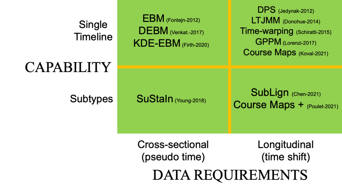
Abbreviations: EBM – Event Based Model; DEBM – Discriminative EBM; KDE-EBM – Kernel Density Estimation EBM; DPS – Disease Progression Score; LTJMM – Latent Time Joint Mixed Model; GPPM – Gaussian Process Progression Model; SuStaIn – Subtype and Stage Inference; SubLign – Subtyping Alignment

The chapter is organised as follows. It starts with a brief discussion of data preprocessing considerations in Section 2 — an important step in medical data analysis. The treatment of D³PMs is separated into models for cross-sectional data (Section 3) and models for longitudinal data (Section 4), each split into approaches that estimate a single timeline of disease progression and those capable of estimating multiple timelines within a dataset (subtyping). Section 5 concludes.

For a detailed timeline of D³PM development including taxonomy and pedigree of key models, see the Appendix.

2. Data preprocessing

This section briefly touches on two common preprocessing steps before fitting a D³PM to data from a progressive condition such as an irreversible chronic disease: controlling for confounding variables, and handling missing data. We refer to input features as biomarkers, and use “covariate” and “confounder” interchangeably. Missing data can refer to irregular/variable visits across individuals, or missing biomarker data due to one or more measurements not being performed for some reason. This section deals with the latter, since longitudinal models can typically handle irregular visits.

Controlling for confounding variables is an important element of any D³PM analysis. This helps to prevent the D³PM from learning non-disease-related patterns such as due to confounding covariates. Confounders can be included as covariates in certain models — to account for that source of variation alongside other variables of interest. Another approach, often used for continuous-valued confounders, is to “regress out” this source of variation prior to fitting a model — to remove non-disease-related signal in the data. This process involves training regression models on data from control participants (who are not expected to develop the disease being studied), then removing the relevant trends from all data. This method can also be applied to categorical risk factors (discrete variables). The canonical example of a potentially confounding variable in neurodegenerative diseases of the brain is age — a key risk factor in many chronic diseases. Removing normal ageing signal is often phrased as “adjusting for” or “controlling for” age.

Handling missing data is an active area of research with a considerable body of literature. Broadly speaking there are two strategies. The easiest is to exclude participants having any missing biomarker (or covariate) data, but this can considerably reduce the sample size of data available for D³PM analysis. The second approach is to impute the missing data, e.g., using group mean values. Imputation can be explicit, or implicit. An example of implicit imputation is in Bayesian models that map data to probabilities, then deal with missing data probabilistically such as in the event-based model [4] where $P(event|x)=0.5$ represents maximal uncertainty such as when a measurement $x$ is missing.

3. Models for cross-sectional data

• Pro: Data-economical.
Require cross-sectional data only. • Con: Limited forecasting utility.
Forecasting requires augmentation with longitudinal data. • Key application(s): assessing disease severity from a single visit, e.g., economical stratification for clinical research/trials.

3.1     S ingle timeline estimation using cross-sectional data

There is only one framework for estimating disease timelines from cross-sectional data: event-based modelling.

3.1.1. Event Based Model

The event-based model (EBM) emerged in 2011 [5, 6]. The concept is simple: in a progressive disease, biomarker measurements only ever get worse, i.e., become increasingly and irreversibly abnormal. Thus, among a cohort of individuals at different stages of a single progressive disease, the cumulative sequence of biomarker abnormality events can be inferred from only a single visit per individual. This requires making a few assumptions: measurements from individuals are independent and represent samples from a single sequence of cumulative abnormality, i.e., a single timeline of disease progression. Such assumptions are commonplace in many statistical analyses of disease progression, and are reasonable approximations to make when analysing data from research studies that typically have strict inclusion and exclusion criteria to focus on a single condition of interest. Unsurprisingly, the event-based model has proven to be extremely powerful, producing insight into many neurodegenerative diseases: sporadic Alzheimer’s disease [7, 8, 9, 10], familial Alzheimer’s disease [6, 11], Huntington’s disease [6, 12], Parkinson’s disease [13], and others [14, 15].

EBM fitting

The first step in fitting an event-based model maps biomarker values to abnormality values, similar to the hypothetical curves of biomarker abnormality proposed in 2010 [1, 2]. The EBM does this probabilistically, using bivariate mixture modelling where individuals can be labelled either as pre-event/normal or post-event/abnormal to allow for (later) events that are yet to occur in patients, and similarly for the possibility of (earlier) events to have occurred in asymptomatic individuals. Various distributions have been proposed for this mixture modelling: combinations of uniform [5, 6], Gaussian [5, 6, 7], and kernel density estimate (KDE) distributions [9]. This is visualised in Figure 2.

Figure 2: Event-based models fit a mixture model to map biomarker values to abnormality probabilities. Left to right shows the convergence of a Kernel Density Estimate (KDE) mixture model. From Firth et al.., 2020 [9] (CC BY 4.0).

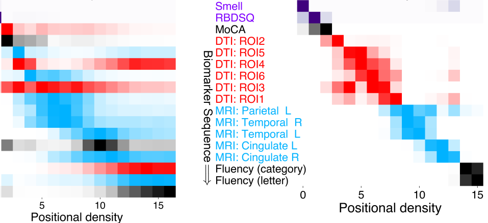
The second step in fitting an EBM over $N$ events is to search the space of $N!$ possible sequences $S$ to reveal the most likely sequence (see [6, 7, 9] for mathematical details). For small $N\lesssim 10$, it can be computationally feasible to perform an exhaustive search over all possible $N!$ sequences to find the maximum likelihood/a posteriori solution. The EBM uses a combination of multiply-initialised gradient ascent, followed by MCMC sampling to estimate uncertainty in the sequence. This results in a model posterior that is a collection of samples from the posterior probability density for each biomarker as a function of sequence position. This is presented as a positional variance diagram [6], such as in Figure 3.

Figure 3: The event-based model posterior is a positional variance diagram showing uncertainty (left-to-right) in the maximum likelihood sequence (top-to-bottom). Parkinson’s disease model from Oxtoby et al.., 2021 [13] (CC BY 4.0).

For further information and to try out EBM tutorials, the reader is directed to the open source kde_ebm package (github.com/ucl-pond/kde_ebm) and disease-progression-modelling.github.io.

3.1.2. Discriminative Event Based Model

The discriminative event-based model (DEBM) was proposed in 2017 by Venkatraghavan et al.. [16]. Whereas the EBM treats data from individuals as observations of a single group-level disease cascade (sequence), the DEBM estimates individual-level sequences and combines them into a group-level description of disease progression. This is done using a Mallow’s Model, which is the ranking/sequencing equivalent of a univariate Gaussian distribution — including estimation of a mean sequence and variance in this mean. Both EBM and DEBM estimate group-level biomarker abnormality using mixture modelling and both approaches directly estimate uncertainty in the sequence.

Additionally, Venkatraghavan et al.. [16, 17] also introduced a pseudo-temporal “disease time” that converts the DEBM posterior into a continuous measure of disease severity.

DEBM fitting

As with the EBM, DEBM model fitting starts with mixture modelling (see Section 3.1.1). Next, a sequence is estimated for each individual by ranking the abnormality probabilities in descending order. A group-level mean sequence (with variance) is estimated by fitting the individual sequences to a Mallow’s Model. For details, see [16, 17] and subsequent innovations to the DEBM. Notably, DEBM is often quicker to fit than EBM, which makes it appealing for high-dimensional extensions, e.g., aiming to estimate voxel-wise atrophy signatures from cross-sectional brain imaging data.

For further information and to try it out, the reader is directed to the open source pyebm package (https://github.com/88vikram/pyebm).

3.2     S ubtyping using cross-sectional data

• Pro: Uncovering heterogeneity without conflating severity with subtype.
Evidence suggests that disease subtypes exist. • Con: Overly simplistic.
Current models ignore comorbidity.

Augmenting the event-based model concept with unsupervised machine learning, Subtype and Stage Inference (SuStaIn) was introduced by Young et al.. [18]. This marriage of clustering to disease progression modelling has proven very powerful and popular, with high-impact results appearing in prominent journals for multiple brain diseases [19, 20, 21], chronic lung disease [22], and knee osteoarthritis [23]. SuStaIn’s popularity is perhaps unsurprising given that it was the first method capable of unravelling spatiotemporal heterogeneity (pathological severity across an organ) from phenotypic heterogeneity (disease subtypes) in progressive conditions using only cross-sectional data.

Figure 4: The concept of Subtype and Stage Inference (SuStaIn). Reproduced from Young et al.., 2018 [18] (CC BY 4.0).

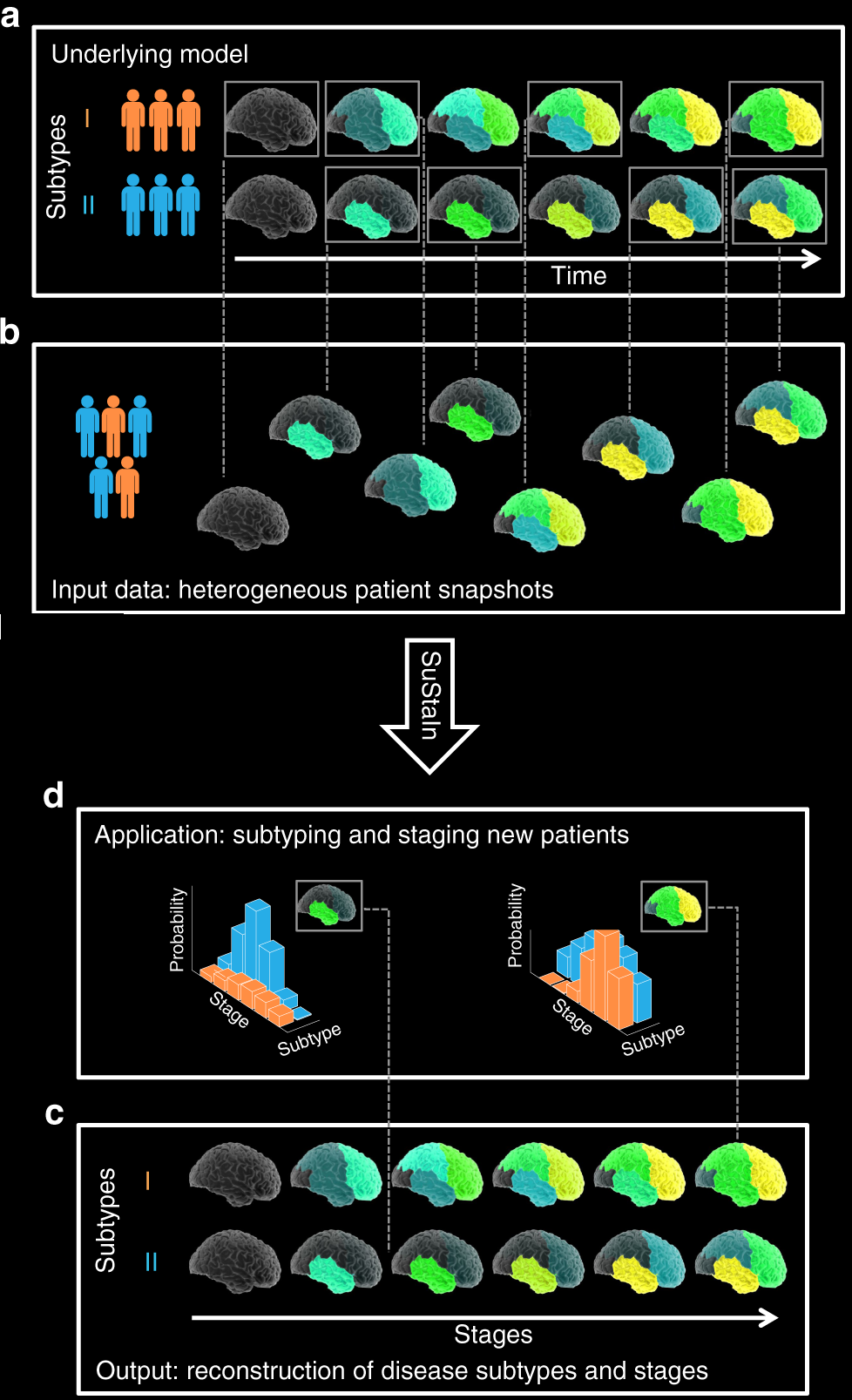
Figure 4 (adapted from [18]) shows the concept behind SuStaIn. SuStaIn iteratively solves the clustering problem from 1 to $N_{\mathrm{S}}^{\mathrm{max}}$ subtypes. The $N_{\mathrm{S}}$ model is fitted by splitting each of the $N_{\mathrm{S}}-1$ subtypes into two clusters then solving the $N_{\mathrm{S}}$-cluster problem, which produces $N_{\mathrm{S}}-1$ candidate $N_{\mathrm{S}}$-cluster models, from which the maximum likelihood model is chosen, then the algorithm continues to $N_{\mathrm{S}}+1$ and so on.

Young et al.. [18] also introduced the z-score event progression model that breaks down individual biomarker events into piecewise linear transitions between z-scores of interest. This removes the need for mixture modelling (such as in event-based modelling) and enables inference to be performed at sub-threshold biomarker values.

SuStaIn fitting

For the user, a SuStaIn analysis is very similar to an event-based model analysis. For further information, the reader is directed to the open source pySuStaIn package [24] (https://github.com/ucl-pond/pySuStaIn), which includes tutorials. As well as the z-score progression model, pySuStaIn includes the various event-based models (see Section 3.1), and the more recent scored-events model for ordinal data [25] such as visual ratings of medical images.

4. Models for longitudinal data

• Pro: Good forecasting utility.
High temporal precision allows individualised forecasting. • Con: Data-heavy.
Require longitudinal data (multiple visits, years). Can be slow to fit. • Key application(s): assessing speed of disease progression; assessing individual variability.

The availability of longitudinal data has fuelled development of more sophisticated D³PMs, inspired by mixed models. Mixed (effect) modelling is the workhorse of longitudinal statistical analysis against a known timeline, e.g., age. Mixed models provide a hierarchical description of individual-level variation (random effects) about group-level trends (fixed effects), hence the common parlance ”mixed effects” models. Many of the D³PMs for longitudinal data discussed below are in fact mixed models with an additional latent-time parameter that characterises the disease timeline. Similar approaches in various fields are known as “self-modelling regression” or “pseudo-time” models. We focus on parametric models, but also mention nonparametric models, and an emerging hybrid discrete-continuous model.

4.1     S ingle timeline estimation using longitudinal data

There are both parametric and non-parametric approaches to estimating disease timelines from longitudinal data. The common goal is to “stitch together” a full disease timeline (decades long) out of relatively short samples from individuals (a few years each) covering a range of severity in symptoms and biomarker abnormality. Some of the earliest work emerged from the medical image registration community, where “warping” images to a common template is one of the first steps in group analyses [26].

Broadly speaking, there are two categories of D³PMs for longitudinal data: time-shifting models and differential equation models. Time-shifting models translate/deform the individual data, metaphorically stitching them together into a quantitative template of disease progression. Differential equation models estimate a statistical model of biomarker dynamics in phase-plane space (position vs velocity), which is subsequently inverted to produce biomarker trajectories.

4.1.1. Explicit models for longitudinal data: latent-time models

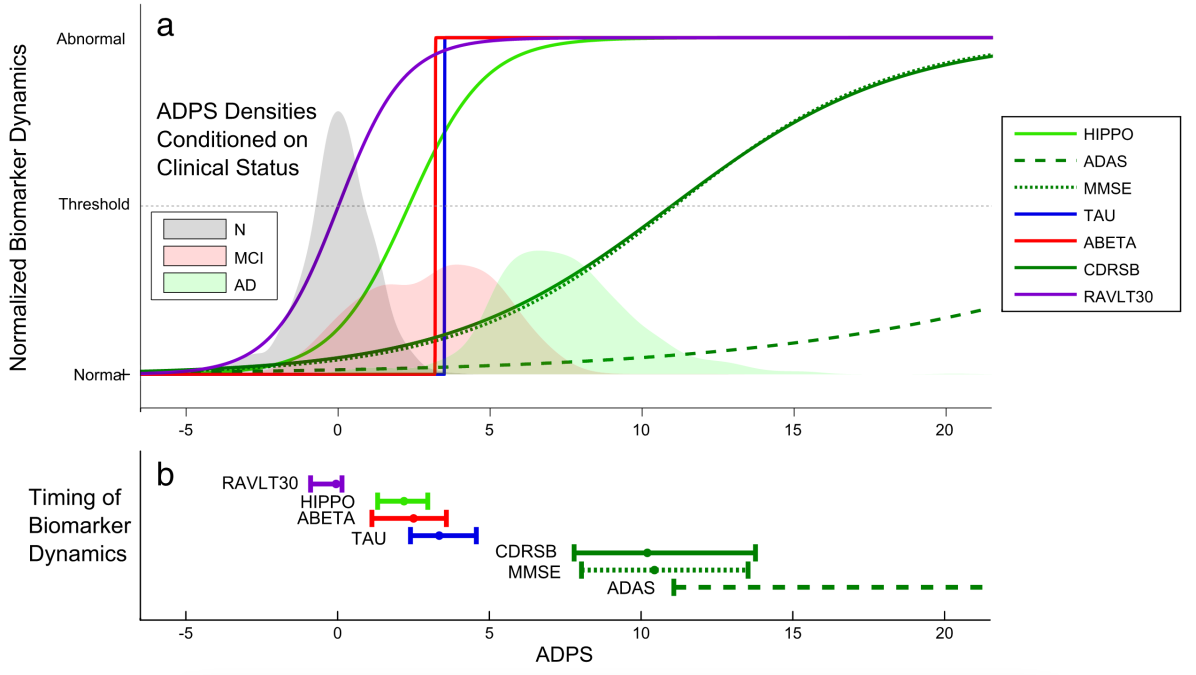
Jedynak, et al. [27] introduced the Disease Progression Score (DPS) model in 2012, which aligns biomarker data from individuals to a group template model using a linear transformation of age into a disease progression score $s_{i}=\alpha_{i}\mathrm{age}+\beta_{i}$. Individuals have their own rate of progression $\alpha_{i}$ (constant over the short observation time) and disease onset $\beta_{i}$. Group level biomarker dynamics are modelled as sigmoid (“S”) curves. A Bayesian extension of the DPS approach (BPS) appeared in 2019 [28]. Code for both the DPS and BPS was released publicly: https://www.nitrc.org/projects/progscore; https://hub.docker.com/r/bilgelm/bayesian-ps-adni/.

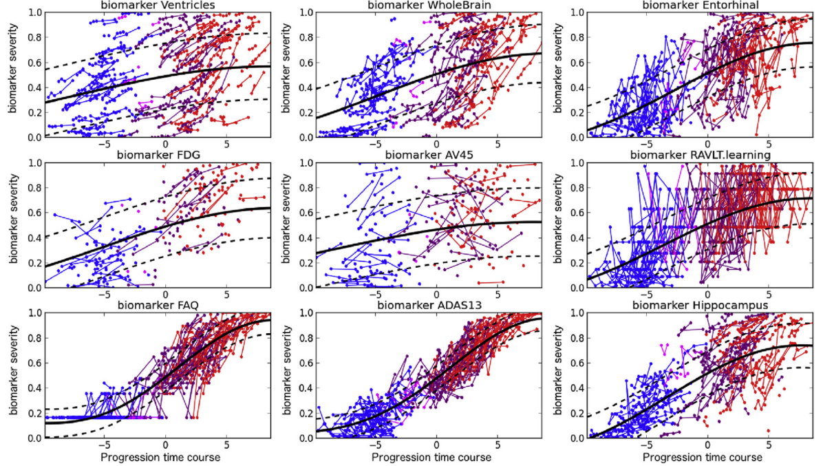
Donohue, et al. [29] introduced a self-modelling regression approach similar to the DPS model in 2014. It was later generalised into the more flexible Latent Time Joint Mixed (effects) Model (LTJMM) [30], which can include covariates as fixed effects and is a flexible Bayesian framework for inference. The LTJMM software was released publicly to https://bitbucket.org/mdonohue/ltjmm.

A non-parametric latent-time mixed model appeared in 2017: the Gaussian process progression model (GPPM) of Lorenzi, et al. [31]. This is a flexible Bayesian approach akin to (parametric) self-modelling regression that doesn’t impose a parametric form for biomarker trajectories. More recent work supplemented the GPPM with a dynamical systems model of molecular pathology spread through the brain [32] that can regularise the GPPM fit to produce a more accurate disease timeline reconstruction that also provides insight into neurodegenerative disease mechanisms (which could be a standalone chapter of this book). The GPPM and GPPM-DS model source code was released publicly via gitlab.inria.fr/epione and tutorials are available at disease-progression-model.github.io.

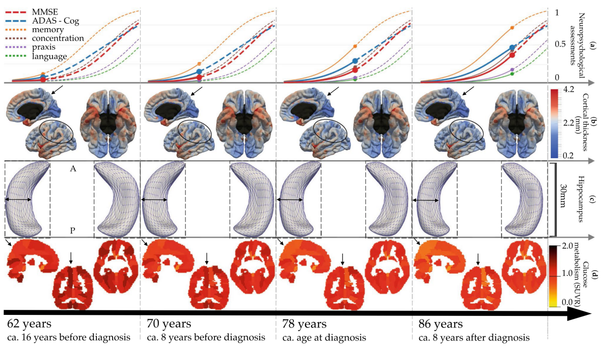
In 2015, Schiratti et al. [33, 34, 35] introduced a general framework for estimating spatiotemporal trajectories for any type of manifold-valued data. The framework is based on Riemannian geometry and a mixed-effects model with time reparametrisation. It was subsequently extended by Koval et al [36] to form the Disease Course Mapping approach (available in the leaspy software package). Disease Course Mapping combines time warping (of age) and inter-biomarker spacing translation. Time warping changes disease progression dynamics — time shift/onset, and acceleration/progression speed — but not the trajectory. Inter-biomarker spacings shift an individual’s trajectory to account for individual differences in the timing and ordering of biomarker trajectories.

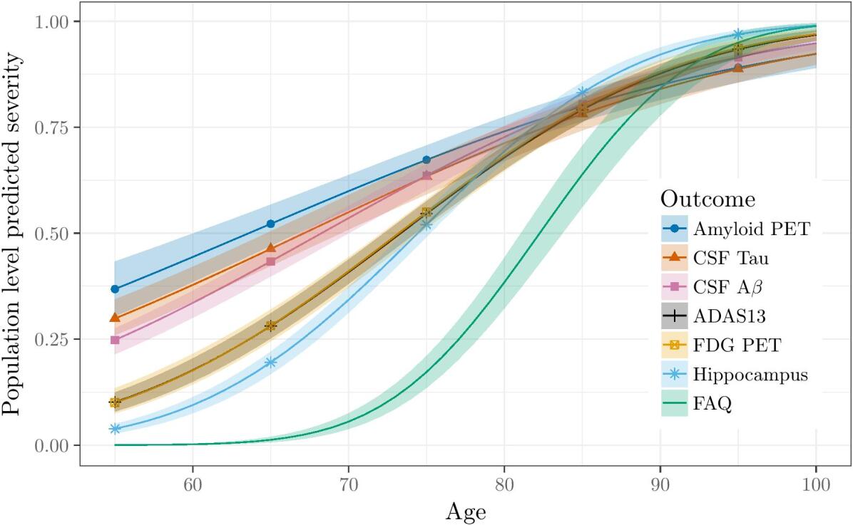
Figures 5 and 6 shows example outputs of these models when trained on data from older people at risk of Alzheimer’s disease, including those with diagnosed mild cognitive impairment and dementia due to probable Alzheimer’s disease.

(a) Alzheimer’s Disease Progression Score (2012) [27]. Reprinted from NeuroImage, Vol 63, Jedynak et al., A computational neurodegenerative disease progression score: Method and results with the Alzheimer’s Disease Neuroimaging Initiative cohort, 1478–1486, ©(2012), with permission from Elsevier.

(b) Gaussian Process Progression Model (2017) [31]. Reprinted from NeuroImage, Vol 190, Lorenzi et al., Probabilistic disease progression modeling to characterize diagnostic uncertainty: Application to staging and prediction in Alzheimer’s disease, 56–68, ©(2019), with permission from Elsevier.

Figure 5: Two examples of D³PMs fit to longitudinal data: Disease Progression Score [27] and Gaussian Process Progression Model [31].

(a) Latent Time Joint Mixed Model (2017) [30]. From [37] (CC BY 4.0).

(b) Alzheimer’s Disease Course Map (2021) [36] (CC BY 4.0).

Figure 6: Two additional examples of D³PMs fit to longitudinal data: Latent Time Joint Mixed Model [30] and Disease Course Mapping [36].

Fitting longitudinal latent-time models

Fitting D³PMs for longitudinal data is more complex than for cross-sectional data, and the software packages discussed above each expect the data in slightly different formats. One thing they have in common is that renormalisation (e.g., min-max or z-score) and reorientation (e.g., to be increasing) is required to put biomarkers on a common scale and direction. In some cases such preprocessing is necessary to ensure/accelerate model convergence. For example, the LTJMM used a quantile transformation followed by inverse Gaussian quantile function to put all biomarkers on a Gaussian scale. For further detailed discussion, including model identifiability, we refer the reader to the original publications cited above and the didactic resources at disease-progression-modelling.github.io.

4.1.2. Implicit models for longitudinal data: differential equation models

Parametric differential equation D³PMs emerged between 2011–2014 [38, 39, 40, 41], receiving a more formal treatment in 2017 [42]. In a hat-tip to Physics, these have also been dubbed “phase-plane” models, which aids in their understanding as a model of velocity (biomarker progression rate) as a function of position (biomarker value). Model fitting is a two-step process whereby the long-time biomarker trajectory is estimated by integrating the phase-plane model estimated on observed data.

A nonparametric differential equation D³PM using Gaussian Processes (GP-DEM) was introduced in 2018 [11]. This added flexibility to the preceding parametric approaches and produced state of the art results in predicting symptom onset in familial Alzheimer’s disease.

Figure 7: Differential equation models, or phase-plane models, for biomarker dynamics involve a three step process: estimate individual-level position and velocity; fit a group-level model of velocity $y$ vs position $x$; integrate to produce a trajectory $x(t)$.
Reprinted by permission from Springer Nature: Oxtoby, N.P. et al., Learning Imaging Biomarker Trajectories from Noisy Alzheimer’s Disease Data Using a Bayesian Multilevel Model. In: Cardoso, M.J., Simpson, I., Arbel, T., Precup, D., Ribbens, A. (eds) Bayesian and grAphical Models for Biomedical Imaging. Lecture Notes in Computer Science, vol 8677, pp. 85–94 ©(2014) [41].

Fitting differential equation models

The concept is shown in Figure 7: differential equation model fitting is a three-step process. First estimate a single value per individual of biomarker “velocity” and “position”, then estimate a group-level differential equation model of velocity $y$ as a function of position $x$, which is integrated/inverted to produce a biomarker trajectory $x(t)$. For example, linear regression can produce estimates of position (e.g., intercept) and velocity (e.g. gradient). Differential equation models can be univariate or multivariate and can include covariates explicitly.

4.1.3. Hybrid discrete-continuous models

Recent work introduced the Temporal EBM (TEBM) [43, 44], which augments event-based modelling with hidden Markov modelling to produce a hybrid discrete-continuous D³PM. This is a halfway house between discrete models (great for medical decision making) and continuous models (great for detailed understanding of disease progression). Trained on data from ADNI, the TEBM revealed the full timeline of the pathophysiological cascade of Alzheimer’s disease, as shown in Figure 8.

Figure 8: Alzheimer’s disease sequence and timeline estimated by a hybrid discrete-continuous D³PM: the Temporal Event-Based Model [43, 44]. Permission to reuse was kindly granted by the authors of [43].

4.2     S ubtyping using longitudinal data

Clustering longitudinal data without a well-defined time axis can be extremely difficult. Jointly estimating latent time for multiple trajectories is an identifiability challenge, i.e., multiple parameter combinations can explain the same data. This is particularly challenging when observations span a relatively small fraction of the full disease timeline, as in age-related neurodegenerative diseases.

Chen et al. [45] introduced SubLign for subtyping and aligning longitudinal disease data. The authors frame the challenge eloquently as having misaligned, interval-censored data: left-censoring from patients being observed only after disease onset; right censoring from patient dropout in more severe disease. SubLign combines a deep generative model (based on a recurrent neural network [46]) for learning individual latent time-shifts and parametric biomarker trajectories using a variational approach, followed by k-means clustering. It was applied to data from a Parkinson’s disease cohort to recover some known clinical phenotypes in new detail.

Poulet and Durrleman [47] recently added mixture-model clustering to the non-linear mixed model approach of Disease Course Mapping [36]. The framework jointly estimates model parameters and subtypes using a modification of the Expectation-Maximisation algorithm. In simulated data experiments their approach outperforms a naive baseline. Experiments on real data in Alzheimer’s disease distinguished rapid from slow clinical progression, with minimal differences in biomarker trajectories.

5. Conclusion

21st century Medicine faces many challenges due to ageing populations worldwide, including increasing socioeconomic burden from age-related brain disorders like Alzheimer’s disease. Many failed clinical trials fuelled intense debate in Neurology in the first decade of this century, culminating in the prominent hypothesis of Alzheimer’s disease progression as a pathophysiological cascade of dynamic biomarker events. This inspired the emergence of Data-Driven Disease Progression Modelling (D³PM) from the Computer Science community during the second decade of the 21st century — an explosion of quantitative models for neurodegenerative disease progression enabling numerous high-impact insights across multiple brain disorders. The community continues to build and share open source code (see Box Appendix) and run machine learning challenges [48, 49, 50]. What will the third decade of the 21st century bring for this exciting subset of machine learning for brain disorders?

Appendix

A taxonomy and pedigree of key D³PM papers is given in Table 1. Box Appendix contains links to open source code for D³PMs.

Table 1: A taxonomy and pedigree of D³PM papers. *Asterisks denote models for cross-sectional data.

Reference (first author only)	Description
Ashford, Curren. Psych. Rep. (2001) [51]	Differential equation
Gomeni, Alz Dem (2011) [52]	Differential equation
Sabuncu, Arch. Neurol. (2011) [38]	Differential equation
Samtani, J. Clin. Pharmacol. (2012) [39]	Differential equation
Jedynak, NIMG (2012) [27]	Progression score (linear)
$\Rightarrow$ Bilgel, IPMI (2015) [53]
$\Rightarrow$ Bilgel, NIMG (2016) [54]	Latent time mixed effects
$\Rightarrow$ Bilgel, Alz Dem DADM (2019) [28]	Bayesian
*Fonteijn, IPMI (2011) [5]; NIMG (2012) [6]	Cumulative events
$\Rightarrow$ *Young, Brain (2014) [7]	Robust for sporadic disease
$\Rightarrow$ *Venkatraghavan, IPMI (2017) [16]; NIMG (2019) [17]	Individual-level
$\Rightarrow$ *Young, Nat Commun (2018) [18]	+Subtyping, +Z-score Model
$\Rightarrow$ *Young, Frontiers (2021) [55]	+Scored Events Model
$\Rightarrow$ *Firth, Alz Dem (2020) [9]	+Nonparametric events
$\Rightarrow$ Wijeratne, ML4H2020, IPMI (2021) [43, 44]	+Transition times
Villemagne, Lancet Neurol (2013) [40]	Differential equation
$\Rightarrow$ Budgeon, Stat. in Med. (2017) [42]	Formalism
Durrleman, Int. J. Comput. Vis. (2013) [56]	Time warping
$\Rightarrow$ Schiratti, NeurIPS (2015) [33]; IPMI (2015) [34]; JMLR (2017) [35]
$\Rightarrow$ Koval, Sci Rep (2021) [36]	Latent time mixed effects
$\Rightarrow$ Poulet, IPMI (2021) [47]	+Subtyping
Donohue, Alz Dem (2014) [29]	Latent time fixed effects
$\Rightarrow$ Li, Stat Meth Med Res (2017) [30]	Latent-time mixed effects
Oxtoby, MICCAI (2014) [57]	Differential equation
$\Rightarrow$ Oxtoby, Brain (2018) [11]	+Nonparametric
Guerrero, NIMG (2016) [58]	Instantiated mixed effects
Leoutsakos, JPAD (2016) [59]	Item Response Theory
Lorenzi, NIMG (2017) [31]	Nonparametric latent time
$\Rightarrow$ Garbarino, IPMI (2019) [60]	+Differential equation
$\Rightarrow$ Garbarino, NIMG (2021) [32]	Formalism
Marinescu, NIMG (2019) [61]	Spatial clustering (c.f. Schiratti/Bilgel)
Petrella, Comp. Math. Meth. Med. (2019) [62]	Differential equation
Abi Nader, Brain Commun. (2021) [63]	Differential equation
Chen, AAAI (2022) [45]	Subtyping

• D³PM tutorials:
https://disease-progression-modelling.github.io • EuroPOND Software Toolbox:
https://europond.github.io/europond-software • KDE EBM:
https://ucl-pond.github.io/kde_ebm • pyEBM:
https://github.com/88vikram/pyebm • leaspy:
https://gitlab.com/icm-institute/aramislab/leaspy • LTJMM:
https://bitbucket.org/mdonohue/ltjmm
https://github.com/mcdonohue/rstanarm • DPS:
source code; docker image • pySuStaIn:
https://ucl-pond.github.io/pySuStaIn • TADPOLE-SHARE (from TADPOLE Challenge [48, 49]):
https://github.com/tadpole-share/tadpole-algorithms

References

- Jack et al [2010] Jack CR, Knopman DS, Jagust WJ, Shaw LM, Aisen PS, Weiner MW, Petersen RC, Trojanowski JQ (2010) Hypothetical model of dynamic biomarkers of the Alzheimer’s pathological cascade. The Lancet Neurology 9(1):119–128, doi:10.1016/S1474-4422(09)70299-6
- Aisen et al [2010] Aisen PS, Petersen RC, Donohue MC, Gamst A, Raman R, Thomas RG, Walter S, Trojanowski JQ, Shaw LM, Beckett LA, Jr CRJ, Jagust W, Toga AW, Saykin AJ, Morris JC, Green RC, Weiner MW (2010) Clinical core of the Alzheimer’s disease neuroimaging initiative: Progress and plans. Alzheimer’s & Dementia 6(3):239 – 246, doi:10.1016/j.jalz.2010.03.006
- Oxtoby et al [2017] Oxtoby NP, Alexander DC, EuroPOND Consortium (2017) Imaging plus X: multimodal models of neurodegenerative disease. Current Opinion in Neurology 30(4), doi:10.1097/WCO.0000000000000460
- Young et al [2015] Young AL, Oxtoby NP, Ourselin S, Schott JM, Alexander DC (2015) A simulation system for biomarker evolution in neurodegenerative disease. Medical Image Analysis 26(1):47–56, doi:10.1016/j.media.2015.07.004
- Fonteijn et al [2011] Fonteijn H, Clarkson M, Modat M, Barnes J, Lehmann M, Ourselin S, Fox N, Alexander D (2011) An event-based disease progression model and its application to familial alzheimer’s disease. In: Székely G, Hahn H (eds) Information Processing in Medical Imaging, Lecture Notes in Computer Science, vol 6801, Springer Berlin / Heidelberg, pp 748–759, doi:10.1007/978-3-642-22092-0_61
- Fonteijn et al [2012] Fonteijn HM, Modat M, Clarkson MJ, Barnes J, Lehmann M, Hobbs NZ, Scahill RI, Tabrizi SJ, Ourselin S, Fox NC, Alexander DC (2012) An event-based model for disease progression and its application in familial Alzheimer’s disease and Huntington’s disease. NeuroImage 60(3):1880 – 1889, doi:10.1016/j.neuroimage.2012.01.062
- Young, Alexandra L., and Oxtoby, Neil P., and Daga, Pankaj, and Cash, David M., and ADNI, and Fox, Nick C., and Ourselin, Sebastien, and Schott, Jonathan M., and Alexander, Daniel C. [2014] Young, Alexandra L, and Oxtoby, Neil P, and Daga, Pankaj, and Cash, David M, and ADNI, and Fox, Nick C, and Ourselin, Sebastien, and Schott, Jonathan M, and Alexander, Daniel C (2014) A data-driven model of biomarker changes in sporadic Alzheimer’s disease. Brain 137(9):2564–2577, doi:10.1093/brain/awu176
- Oxtoby et al [2017] Oxtoby NP, Garbarino S, Firth NC, Warren JD, Schott JM, Alexander DC, FtADNI (2017) Data-Driven Sequence of Changes to Anatomical Brain Connectivity in Sporadic Alzheimer’s Disease. Frontiers in Neurology 8:580, doi:10.3389/fneur.2017.00580
- Firth et al [2020] Firth NC, Primativo S, Brotherhood E, Young AL, Yong KX, Crutch SJ, Alexander DC, Oxtoby NP (2020) Sequences of cognitive decline in typical Alzheimer’s disease and posterior cortical atrophy estimated using a novel event-based model of disease progression. Alzheimer’s & Dementia 16(7):965–973, doi:10.1002/alz.12083
- Janelidze et al [2021] Janelidze S, Berron D, Smith R, Strandberg O, Proctor NK, Dage JL, Stomrud E, Palmqvist S, Mattsson-Carlgren N, Hansson O (2021) Associations of Plasma Phospho-Tau217 Levels With Tau Positron Emission Tomography in Early Alzheimer Disease. JAMA Neurology 78(2):149–156, doi:10.1001/jamaneurol.2020.4201
- Oxtoby et al [2018] Oxtoby NP, Young AL, Cash DM, Benzinger TLS, Fagan AM, Morris JC, Bateman RJ, Fox NC, Schott JM, Alexander DC (2018) Data-driven models of dominantly-inherited alzheimer’s disease progression. Brain 141(5):1529–1544, doi:10.1093/brain/awy050
- Wijeratne et al [2018] Wijeratne PA, Young AL, Oxtoby NP, Marinescu RV, Firth NC, Johnson EB, Mohan A, Sampaio C, Scahill RI, Tabrizi SJ, Alexander DC (2018) An image-based model of brain volume biomarker changes in Huntington’s disease. Annals of Clinical and Translational Neurology 5(5):570–582, doi:10.1002/acn3.558
- Oxtoby et al [2021] Oxtoby NP, Leyland LA, Aksman LM, Thomas GEC, Bunting EL, Wijeratne PA, Young AL, Zarkali A, Tan MMX, Bremner FD, Keane PA, Morris HR, Schrag AE, Alexander DC, Weil RS (2021) Sequence of clinical and neurodegeneration events in Parkinson’s disease progression. Brain 144(3):975–988, doi:10.1093/brain/awaa461
- Eshaghi et al [2018] Eshaghi A, Marinescu RV, Young AL, Firth NC, Prados F, Jorge Cardoso M, Tur C, De Angelis F, Cawley N, Brownlee WJ, De Stefano N, Laura Stromillo M, Battaglini M, Ruggieri S, Gasperini C, Filippi M, Rocca MA, Rovira A, Sastre-Garriga J, Geurts JJG, Vrenken H, Wottschel V, Leurs CE, Uitdehaag B, Pirpamer L, Enzinger C, Ourselin S, Gandini Wheeler-Kingshott CA, Chard D, Thompson AJ, Barkhof F, Alexander DC, Ciccarelli O (2018) Progression of regional grey matter atrophy in multiple sclerosis. Brain 141(6):1665–1677, doi:10.1093/brain/awy088
- Firth et al [2018] Firth NC, Startin CM, Hithersay R, Hamburg S, Wijeratne PA, Mok KY, Hardy J, Alexander DC, Consortium TL, Strydom A (2018) Aging related cognitive changes associated with Alzheimer’s disease in Down syndrome. Annals of Clinical and Translational Neurology 5(6):741–751, doi:10.1002/acn3.571
- Venkatraghavan et al [2017] Venkatraghavan V, Bron EE, Niessen WJ, Klein S (2017) A Discriminative Event Based Model for Alzheimer’s Disease Progression Modeling. In: Niethammer M, Styner M, Aylward S, Zhu H, Oguz I, Yap PT, Shen D (eds) Information Processing in Medical Imaging, Springer International Publishing, Cham, Lecture Notes in Computer Science, pp 121–133, doi:10.1007/978-3-319-59050-9_10
- Venkatraghavan et al [2019] Venkatraghavan V, Bron EE, Niessen WJ, Klein S (2019) Disease progression timeline estimation for alzheimer’s disease using discriminative event based modeling. NeuroImage 186:518–532, doi:10.1016/j.neuroimage.2018.11.024
- Young and et al. [2018] Young AL, et al (2018) Uncovering the heterogeneity and temporal complexity of neurodegenerative diseases with subtype and stage inference. Nature Communications 9(1):4273, doi:10.1038/s41467-018-05892-0
- Vogel et al [2021] Vogel JW, Young AL, Oxtoby NP, Smith R, Ossenkoppele R, Strandberg OT, La Joie R, Aksman LM, Grothe MJ, Iturria-Medina Y, the Alzheimer’s Disease Neuroimaging Initiative, Pontecorvo MJ, Devous MD, Rabinovici GD, Alexander DC, Lyoo CH, Evans AC, Hansson O (2021) Four distinct trajectories of tau deposition identified in alzheimer’s disease. Nature Medicine doi:10.1038/s41591-021-01309-6
- Eshaghi et al [2021] Eshaghi A, Young AL, Wijeratne PA, Prados F, Arnold DL, Narayanan S, Guttmann CRG, Barkhof F, Alexander DC, Thompson AJ, Chard D, Ciccarelli O (2021) Identifying multiple sclerosis subtypes using unsupervised machine learning and MRI data. Nature Communications 12(1):2078, doi:10.1038/s41467-021-22265-2
- Collij et al [2022] Collij LE, Salvadó G, Wottschel V, Mastenbroek SE, Schoenmakers P, Heeman F, Aksman L, Wink AM, Berckel BNM, Flier WMvd, Scheltens P, Visser PJ, Barkhof F, Haller S, Gispert JD, Alves IL, Initiative ftADN, Study ftA (2022) Spatial-Temporal Patterns of -Amyloid Accumulation: A Subtype and Stage Inference Model Analysis. Neurology 98(17):e1692–e1703, doi:10.1212/WNL.0000000000200148
- Young et al [2020] Young AL, Bragman FJS, Rangelov B, Han MK, Galbán CJ, Lynch DA, Hawkes DJ, Alexander DC, Hurst JR (2020) Disease progression modeling in chronic obstructive pulmonary disease. American Journal of Respiratory and Critical Care Medicine 201(3):294–302, doi:10.1164/rccm.201908-1600OC
- Li et al [2021] Li M, Lan L, Luo J, Peng L, Li X, Zhou X (2021) Identifying the Phenotypic and Temporal Heterogeneity of Knee Osteoarthritis: Data From the Osteoarthritis Initiative. Frontiers in Public Health 9, doi:10.3389/fpubh.2021.726140
- Aksman et al [2021] Aksman LM, Wijeratne PA, Oxtoby NP, Eshaghi A, Shand C, Altmann A, Alexander DC, Young AL (2021) pySuStaIn: A Python implementation of the Subtype and Stage Inference algorithm. SoftwareX 16:100811, doi:10.1016/j.softx.2021.100811
- Young et al [2021] Young AL, Vogel JW, Aksman LM, Wijeratne PA, Eshaghi A, Oxtoby NP, Williams SCR, Alexander DC, ftADNI (2021) Ordinal sustain: Subtype and stage inference for clinical scores, visual ratings, and other ordinal data. Frontiers in Artificial Intelligence 4:111, doi:10.3389/frai.2021.613261
- Durrleman et al [2009] Durrleman S, Pennec X, Trouvé A, Gerig G, Ayache N (2009) Spatiotemporal atlas estimation for developmental delay detection in longitudinal datasets. In: Yang GZ, Hawkes D, Rueckert D, Noble A, Taylor C (eds) Medical Image Computing and Computer-Assisted Intervention – MICCAI 2009, Springer Berlin Heidelberg, Berlin, Heidelberg, pp 297–304, doi:10.1007/978-3-642-04268-3_37
- Jedynak et al [2012] Jedynak BM, Lang A, Liu B, Katz E, Zhang Y, Wyman BT, Raunig D, Jedynak CP, Caffo B, Prince JL (2012) A computational neurodegenerative disease progression score: Method and results with the Alzheimer’s disease neuroimaging initiative cohort. NeuroImage 63(3):1478–1486, doi:10.1016/j.neuroimage.2012.07.059
- Bilgel et al [2019] Bilgel M, Jedynak BM, Initiative ADN (2019) Predicting time to dementia using a quantitative template of disease progression. Alzheimer’s & Dementia: Diagnosis, Assessment & Disease Monitoring 11(1):205–215, doi:10.1016/j.dadm.2019.01.005
- Donohue et al [2014] Donohue MC, Jacqmin-Gadda H, Goff ML, Thomas RG, Raman R, Gamst AC, Beckett LA, Jr CRJ, Weiner MW, Dartigues JF, Aisen PS (2014) Estimating long-term multivariate progression from short-term data. Alzheimer’s & Dementia 10(5, Supplement):S400 – S410, doi:10.1016/j.jalz.2013.10.003
- Li et al [2019] Li D, Iddi S, Thompson WK, Donohue MC (2019) Bayesian latent time joint mixed effect models for multicohort longitudinal data. Statistical Methods in Medical Research 28(3):835–845, doi:10.1177/0962280217737566
- Lorenzi et al [2019] Lorenzi M, Filippone M, Frisoni GB, Alexander DC, Ourselin S (2019) Probabilistic disease progression modeling to characterize diagnostic uncertainty: Application to staging and prediction in Alzheimer’s disease. NeuroImage 190:56–68, doi:10.1016/j.neuroimage.2017.08.059
- Garbarino and Lorenzi [2021] Garbarino S, Lorenzi M (2021) Investigating hypotheses of neurodegeneration by learning dynamical systems of protein propagation in the brain. NeuroImage 235:117980, doi:10.1016/j.neuroimage.2021.117980
- Schiratti et al [2015a] Schiratti JB, Allassonnière S, Colliot O, Durrleman S (2015a) Learning spatiotemporal trajectories from manifold-valued longitudinal data. In: Advances in Neural Information Processing Systems, Curran Associates, Inc., vol 28, URL https://proceedings.neurips.cc/paper/2015/hash/186a157b2992e7daed3677ce8e9fe40f-Abstract.html
- Schiratti et al [2015b] Schiratti JB, Allassonnière S, Routier A, Colliot O, Durrleman S (2015b) A Mixed-Effects Model with Time Reparametrization for Longitudinal Univariate Manifold-Valued Data. In: Ourselin S, Alexander DC, Westin CF, Cardoso MJ (eds) Information Processing in Medical Imaging, Springer International Publishing, Cham, Lecture Notes in Computer Science, pp 564–575, doi:10.1007/978-3-319-19992-4_44
- Schiratti et al [2017] Schiratti JB, Allassonnière S, Colliot O, Durrleman S (2017) A Bayesian mixed-effects model to learn trajectories of changes from repeated manifold-valued observations. Journal of Machine Learning Research 3:1–48
- Koval et al [2021] Koval I, Bône A, Louis M, Lartigue T, Bottani S, Marcoux A, Samper-González J, Burgos N, Charlier B, Bertrand A, Epelbaum S, Colliot O, Allassonnière S, Durrleman S (2021) AD Course Map charts Alzheimer’s disease progression. Scientific Reports 11(1):8020, doi:10.1038/s41598-021-87434-1
- Li et al [2017] Li D, Iddi S, Thompson WK, Donohue MC (2017) Bayesian latent time joint mixed effect models for multicohort longitudinal data. arXiv 1703.10266v2, doi:10.48550/arXiv.1703.10266
- Sabuncu et al [2011] Sabuncu M, Desikan R, Sepulcre J, Yeo B, Liu H, Schmansky N, Reuter M, Weiner M, Buckner R, Sperling R (2011) The dynamics of cortical and hippocampal atrophy in Alzheimer disease. Archives of Neurology 68(8):1040, doi:10.1001/archneurol.2011.167
- Samtani et al [2012] Samtani MN, Farnum M, Lobanov V, Yang E, Raghavan N, DiBernardo A, Narayan V, Initiative AtADN (2012) An Improved Model for Disease Progression in Patients From the Alzheimer’s Disease Neuroimaging Initiative. The Journal of Clinical Pharmacology 52(5):629–644, doi:10.1177/0091270011405497
- Villemagne et al [2013] Villemagne VL, Burnham S, Bourgeat P, Brown B, Ellis KA, Salvado O, Szoeke C, Macaulay SL, Martins R, Maruff P, Ames D, Rowe CC, Masters CL (2013) Amyloid deposition, neurodegeneration, and cognitive decline in sporadic Alzheimer’s disease: a prospective cohort study. The Lancet Neurology 12(4):357 – 367, doi:10.1016/S1474-4422(13)70044-9
- Oxtoby et al [2014] Oxtoby NP, Young AL, Fox NC, Daga P, Cash DM, Ourselin S, Schott JM, Alexander DC (2014) Learning imaging biomarker trajectories from noisy alzheimer’s disease data using a bayesian multilevel model. In: Cardoso MJ, Simpson I, Arbel T, Precup D, Ribbens A (eds) Bayesian and grAphical Models for Biomedical Imaging, Lecture Notes in Computer Science, vol 8677, Springer International Publishing, pp 85–94, doi:10.1007/978-3-319-12289-2_8
- Budgeon et al [2017] Budgeon C, Murray K, Turlach B, Baker S, Villemagne V, Burnham S, Initiative ftADN (2017) Constructing longitudinal disease progression curves using sparse, short-term individual data with an application to Alzheimer’s disease. Statistics in Medicine 36(17):2720–2734, doi:10.1002/sim.7300
- Wijeratne and Alexander [2020] Wijeratne PA, Alexander DC (2020) Learning transition times in event sequences: the Event-Based Hidden Markov Model of disease progression. doi:10.48550/arXiv.2011.01023, Machine Learning for Health (ML4H) 2020.
- Wijeratne and Alexander [2021] Wijeratne PA, Alexander DC (2021) Learning Transition Times in Event Sequences: The Temporal Event-Based Model of Disease Progression. In: Feragen A, Sommer S, Schnabel J, Nielsen M (eds) Information Processing in Medical Imaging, Springer International Publishing, Cham, Lecture Notes in Computer Science, pp 583–595, doi:10.1007/978-3-030-78191-0_45
- Chen et al [2022] Chen IY, Krishnan RG, Sontag D (2022) Clustering Interval-Censored Time-Series for Disease Phenotyping. Proceedings of the AAAI Conference on Artificial Intelligence 36(6):6211–6221, doi:10.1609/aaai.v36i6.20570
- Rumelhart et al [1986] Rumelhart DE, Hinton GE, Williams RJ (1986) Learning representations by back-propagating errors. Nature 323(6088):533–536, doi:10.1038/323533a0
- Poulet and Durrleman [2021] Poulet PE, Durrleman S (2021) Mixture Modeling for Identifying Subtypes in Disease Course Mapping. In: Feragen A, Sommer S, Schnabel J, Nielsen M (eds) Information Processing in Medical Imaging, Springer International Publishing, Cham, Lecture Notes in Computer Science, pp 571–582, doi:10.1007/978-3-030-78191-0_44
- Marinescu et al [2018] Marinescu RV, Oxtoby NP, Young AL, Bron EE, Toga AW, Weiner MW, Barkhof F, Fox NC, Klein S, Alexander DC, Consortium tE (2018) TADPOLE Challenge: Prediction of Longitudinal Evolution in Alzheimer’s Disease. doi:10.48550/arXiv.1805.03909
- Marinescu et al [2021] Marinescu RV, Oxtoby NP, Young AL, Bron EE, et al, Alexander DC (2021) The Alzheimer’s Disease Prediction Of Longitudinal Evolution (TADPOLE) Challenge: Results after 1 Year Follow-up. Machine Learning for Biomedical Imaging 1:1–10, URL https://www.melba-journal.org/papers/2021:019.html
- Bron et al [2022] Bron EE, Klein S, Reinke A, Papma JM, Maier-Hein L, Alexander DC, Oxtoby NP (2022) Ten years of image analysis and machine learning competitions in dementia. NeuroImage 253:119083, doi:10.1016/j.neuroimage.2022.119083
- Ashford and Schmitt [2001] Ashford JW, Schmitt FA (2001) Modeling the time-course of Alzheimer dementia. Current Psychiatry Reports 3(1):20–28, doi:10.1007/s11920-001-0067-1
- Gomeni et al [2012] Gomeni R, Simeoni M, Zvartau-Hind M, Irizarry MC, Austin D, Gold M (2012) Modeling alzheimer’s disease progression using the disease system analysis approach. Alzheimer’s & Dementia 8(1):39–50, doi:10.1016/j.jalz.2010.12.012
- Bilgel et al [2015] Bilgel M, Jedynak B, Wong DF, Resnick SM, Prince JL (2015) Temporal Trajectory and Progression Score Estimation from Voxelwise Longitudinal Imaging Measures: Application to Amyloid Imaging. In: Ourselin S, Alexander DC, Westin CF, Cardoso MJ (eds) Information Processing in Medical Imaging, Springer International Publishing, Cham, Lecture Notes in Computer Science, pp 424–436, doi:10.1007/978-3-319-19992-4_33
- Bilgel et al [2016] Bilgel M, Prince JL, Wong DF, Resnick SM, Jedynak BM (2016) A multivariate nonlinear mixed effects model for longitudinal image analysis: Application to amyloid imaging. NeuroImage 134:658–670, doi:10.1016/j.neuroimage.2016.04.001
- Young et al [2021] Young AL, Vogel JW, Aksman LM, Wijeratne PA, Eshaghi A, Oxtoby NP, Williams SCR, Alexander DC, ftADNI (2021) Ordinal SuStaIn: Subtype and Stage Inference for Clinical Scores, Visual Ratings, and Other Ordinal Data. Frontiers in Artificial Intelligence 4(613261), doi:10.3389/frai.2021.613261
- Durrleman et al [2013] Durrleman S, Pennec X, Trouvé A, Braga J, Gerig G, Ayache N (2013) Toward a Comprehensive Framework for the Spatiotemporal Statistical Analysis of Longitudinal Shape Data. International Journal of Computer Vision 103(1):22–59, doi:10.1007/s11263-012-0592-x
- Oxtoby et al [2014] Oxtoby NP, Young AL, Fox NC, Daga P, Cash DM, Ourselin S, Schott JM, Alexander DC (2014) Learning imaging biomarker trajectories from noisy alzheimer’s disease data using a bayesian multilevel model. In: Cardoso MJ, Simpson I, Arbel T, Precup D, Ribbens A (eds) Bayesian and grAphical Models for Biomedical Imaging, Springer International Publishing, Cham, pp 85–94, doi:10.1007/978-3-319-12289-2_8
- Guerrero et al [2016] Guerrero R, Schmidt-Richberg A, Ledig C, Tong T, Wolz R, Rueckert D (2016) Instantiated mixed effects modeling of Alzheimer’s disease markers. NeuroImage 142:113–125, doi:10.1016/j.neuroimage.2016.06.049
- Leoutsakos et al [2016] Leoutsakos JM, Gross AL, Jones RN, Albert MS, Breitner JCS (2016) ‘Alzheimer’s progression score’: Development of a Biomarker Summary Outcome for AD Prevention Trials. Journal of Prevention of Alzheimer’s Disease 3(4):229–235, doi:10.14283/jpad.2016.120
- Garbarino and Lorenzi [2019] Garbarino S, Lorenzi M (2019) Modeling and Inference of Spatio-Temporal Protein Dynamics Across Brain Networks. In: Chung ACS, Gee JC, Yushkevich PA, Bao S (eds) Information Processing in Medical Imaging, Springer International Publishing, Cham, Lecture Notes in Computer Science, pp 57–69, doi:10.1007/978-3-030-20351-1_5
- Marinescu et al [2019] Marinescu RV, Eshaghi A, Lorenzi M, Young AL, Oxtoby NP, Garbarino S, Crutch SJ, Alexander DC (2019) DIVE: A spatiotemporal progression model of brain pathology in neurodegenerative disorders. NeuroImage 192:166–177, doi:10.1016/j.neuroimage.2019.02.053
- Petrella et al [2019] Petrella JR, Hao W, Rao A, Doraiswamy PM (2019) Computational Causal Modeling of the Dynamic Biomarker Cascade in Alzheimer’s Disease. Computational and Mathematical Methods in Medicine 2019:e6216530, doi:10.1155/2019/6216530
- Abi Nader et al [2021] Abi Nader C, Ayache N, Frisoni GB, Robert P, Lorenzi M, for the Alzheimer’s Disease Neuroimaging Initiative (2021) Simulating the outcome of amyloid treatments in Alzheimer’s disease from imaging and clinical data. Brain Communications 3(2):fcab091, doi:10.1093/braincomms/fcab091