Morphological signatures of mergers in the TNG50 simulation and the Kilo-Degree Survey: the merger fraction from dwarfs to Milky Way-like galaxies

Abstract

Using the TNG50 cosmological simulation and observations from the Kilo-Degree Survey (KiDS), we investigate the connection between galaxy mergers and optical morphology in the local Universe over a wide range of galaxy stellar masses ($8.5\leqslant\log(M_{\ast}/\text{M}_{\odot})\leqslant 11$). To this end, we have generated over 16 000 synthetic images of TNG50 galaxies designed to match KiDS observations, including the effects of dust attenuation and scattering, and used the statmorph code to measure various image-based morphological diagnostics in the $r$-band for both data sets. Such measurements include the Gini–$M_{20}$ and concentration–asymmetry–smoothness statistics. Overall, we find good agreement between the optical morphologies of TNG50 and KiDS galaxies, although the former are slightly more concentrated and asymmetric than their observational counterparts. Afterwards, we trained a random forest classifier to identify merging galaxies in the simulation (including major and minor mergers) using the morphological diagnostics as the model features, along with merger statistics from the merger trees as the ground truth. We find that the asymmetry statistic exhibits the highest feature importance of all the morphological parameters considered. Thus, the performance of our algorithm is comparable to that of the more traditional method of selecting highly asymmetric galaxies. Finally, using our trained model, we estimate the galaxy merger fraction in both our synthetic and observational galaxy samples, finding in both cases that the galaxy merger fraction increases steadily as a function of stellar mass.

1 Introduction

It is now accepted, within the $\Lambda$ Cold Dark Matter ($\Lambda$CDM) model, that galaxy mergers play a fundamental role in the formation and evolution of galaxies (White & Rees, 1978). These events change the nature of galaxies in a number of ways: post-mergers exhibit a diminished central metallicity (e.g. Kewley et al., 2006; Scudder et al., 2012); while merging galaxies not only have both enhanced morphological disturbances (e.g. Conselice, 2003; Lotz et al., 2008; Casteels et al., 2014) and star formation rates (e.g. Patton et al., 2013; Thorp et al., 2019) in comparison to non-mergers, but also tend to exhibit active galactic nuclei (e.g. Ellison et al., 2011; Ellison et al., 2019).

Modern cosmological simulations, such as those from the EAGLE (Schaye et al., 2015; Crain et al., 2015), Illustris (Vogelsberger et al., 2014a, b; Genel et al., 2014; Sijacki et al., 2015), IllustrisTNG (Marinacci et al., 2018; Naiman et al., 2018; Nelson et al., 2018; Pillepich et al., 2018b; Springel et al., 2018; Nelson et al., 2019a) and Horizon-AGN (Dubois et al., 2014) projects, have been able not only to corroborate most observational findings about mergers, but also to provide additional insights that can be used to inform and interpret observations. For example, one of the most interesting and studied topics is the determination of the galaxy merger rate, namely, the number of mergers per unit time. A proper determination of this quantity is important to fully understand the role of interactions in galactic structure and star formation rates, as well as to test hierarchical galaxy formation models.

Theoretically, the merger rate is estimated via semi-empirical (e.g. Stewart et al. 2009; Hopkins et al. 2010) and semi-analytic (e.g. Guo & White 2008) models as well as using hydrodynamic cosmological simulations (e.g. Rodriguez-Gomez et al. 2015). In particular, Rodriguez-Gomez et al. (2015) used the Illustris simulation to quantify the galaxy-galaxy merger rate as a function of stellar mass, merger mass ratio, and redshift, finding that it increases steadily with stellar mass and redshift, while being in good agreement with observational constraints for both intermediate-sized and massive galaxies.

On the observational side, it is important to note that the merger rate cannot be estimated directly. Instead, the merger fraction, i.e. the fraction of galaxies observed to be undergoing a merger, must be computed first, and then translated into a rate dividing by an appropriate observability time-scale reflecting the merging detection period. The merger fraction is typically computed by using observations of close pairs or morphologically disturbed galaxies.

Close-pair merger candidates have been identified by several authors (e.g. Lin et al. 2004; Propris et al. 2005; Kartaltepe et al. 2007; Besla et al. 2018; Duncan et al. 2019) as galaxies with a neighbour within a small projected angular separation and with a small line-of-sight relative radial velocity. Alternatively, since there is a close connection between galactic structure and merging processes, some types of morphologically disturbed galaxies are also considered to be ideal merger candidates.

In particular, non-parametric morphological diagnostics, such as the concentration–asymmetry–smoothness (CAS, Conselice 2003), Gini–$M_{20}$ (Lotz et al., 2004), and multimode–intensity–deviation (MID, Freeman et al., 2013) statistics, have been successfully used to identify galaxy mergers and to study, among other things, the evolution of the observational merger rate (e.g. Lotz et al., 2011), its dependence on galaxy stellar mass (e.g. Casteels et al., 2014), as well as to obtain the galaxy merger rate and merging time-scales from hydrodynamical simulations, allowing direct comparisons with observational estimates (e.g. Bignone et al., 2016; Whitney et al., 2021).

More recently, machine learning and deep learning methods have been adopted, for the same purpose, as an alternative to more standard methods. For instance, Snyder et al. (2019) considered a high-mass galaxy sample from the original Illustris simulation to create, based on image-based morphological calculations and merger statistics, a training data set that was fed to a random forest classifier. The resulting model was then used to perform observational and theoretical estimates of the merger rate as a function of redshift. This method was also recently used to perform merger classifications on JWST-like simulated images (Rose et al., 2022). Similarly, Nevin et al. (2019) combined non-parametric morphological statistics with a linear discriminant analysis (LDA) classifier to characterize simulated mergers and found that the LDA classifier outperformed the individual metrics.

Furthermore, convolutional neural networks have been adopted to study galaxy morphology in different contexts. To list a few, they have been applied to differentiate disk galaxies from bulge-dominated systems in both observations and cosmological simulations (Huertas-Company et al., 2015, 2019), to identify merging galaxies in cosmological simulations (Ćiprijanović et al., 2020), to determine the effect of merging events on the star formation rates of galaxies (Pearson et al., 2019), to predict the stage of interaction on synthetic galaxy images and to assess the degree of realism and post-processing needed on these synthetic images to perform adequate deep learning estimations (Bottrell et al., 2019), and to identify high-mass major merger events in observations and simulations and subsequently estimate the merger fraction (Wang et al., 2020).

Despite the well-established link between mergers and morphology in massive galaxies, the incidence and effects of mergers in dwarf galaxies $(M_{\ast}<10^{9.5}\,\mathrm{M}_{\odot})$ are more uncertain. This is an important topic to explore, since galaxy mergers can be transformative events and dwarfs represent the majority of the galaxy population. For example, Casteels et al. (2014) studied a local galaxy sample at $z<0.2$ and $10^{8}\,\mathrm{M}_{\odot}<M_{\ast}<10^{11.5}\,\mathrm{M}_{\odot}$ to infer the mass-dependent galaxy merger fraction and merger rate by measuring the asymmetry parameter from galaxy images. Their estimated major merger fraction is a decreasing function of stellar mass, falling from $4\%$ at $M_{\ast}\sim 10^{9}\,\mathrm{M}_{\odot}$ to $2\%$ at $M_{\ast}\sim 10^{11}\,\mathrm{M}_{\odot}$. This finding suggests that galaxy interactions might become increasingly important for lower-mass galaxies.

Similarly, Besla et al. (2018) computed the frequency of companions for a low-redshift dwarf galaxy ($0.013<z<0.0252$; $2\times 10^{8}\,\text{M}_{\odot}<M_{\ast}<5\times 10^{9}\,\text{M}_{\odot}$) sample from the Sloan Digital Sky Survey (SDSS), comparing it to a mock galaxy sample from the original Illustris simulation. One of the goals of their study was to estimate the major pair fraction as a function of stellar mass, finding that this quantity increases slowly with stellar mass, but does not follow the decreasing trend reported by Casteels et al. (2014). Motivated by such opposing results, in this paper we revisit the topic of the mass-dependent merger fraction, with an emphasis on the regime of dwarf galaxies.

In this work, we use the TNG$50$ simulation from the IllustrisTNG project to investigate the galaxy merger fraction at the low-mass end ($8.5\leqslant\log(M_{\ast}/\text{M}_{\odot})\leqslant 11$), and whether it can be inferred statistically from morphological disturbances in large samples of galaxies. For this purpose, we generate a large set of synthetic images of TNG$50$ galaxies, including the effects of dust attenuation and scattering, designed to match observations from the Kilo-Degree Survey (KiDS). We then calculate several image-based morphological statistics for both the real and simulated galaxy samples, and explore the connection between morphology and mergers in the simulation. Instead of solely using the asymmetry statistic as a merger indicator, we follow a similar approach to that of Snyder et al. (2019) and train a random forest classifier using several non-parametric morphological indicators as the model features and merger statistics from the simulation merger trees as the ground truth. The trained models are then applied to the observational sample in order to estimate the local merger fraction as a function of galaxy mass in the real Universe.

This paper is structured as follows. In LABEL:sub:The_IllustrisTNGsimulations we briefly review the IllustrisTNG simulations, and in LABEL:sub:Observationalsample and 2.3 we describe the observational and simulated galaxy samples used in our analysis. In Sections 2.4 and 2.5 we describe the design and generation of synthetic images from the simulated sample, as well as the source segmentation and deblending procedures. Subsequently, in Section 2.6 we present the morphological diagnostics measured on both galaxy samples. In Section 2.7 we define our merging and non-merging simulated samples, and in LABEL:sub:Randomforest_classification we describe the training and calibration of our random forest classifier. Our main results are given in Section 3, where we examine the morphological differences between our observational and synthetic galaxy samples (Section 3.1) as well as between merging and non-merging simulated galaxies (Section 3.2), evaluate the performance of our random forest classifier (Section 3.3), and present the resulting mass-dependent merger fraction (Section 3.4). Finally, we discuss our results in Section 4 and present our conclusions in Section 5.

2 Methodology

2.1 The IllustrisTNG simulations

The IllustrisTNG project is a suite of $N$-body magneto-hydrodynamical cosmological simulations that model dark and baryonic matter assuming a $\Lambda$CDM framework (Marinacci et al., 2018; Naiman et al., 2018; Nelson et al., 2018; Pillepich et al., 2018b; Springel et al., 2018; Nelson et al., 2019a). The simulation suite consists of three cubic volumes with periodic boundary conditions: TNG50, TNG100, and TNG300, which measure 51.7, 110.7, and 302.6 Mpc on a side, respectively.

In this work we use the highest resolution version of the TNG$50$ simulation (Pillepich et al., 2019; Nelson et al., 2019b), which has a volume of $\quantity($51.7\text{\,}\mathrm{Mpc}$)^{3}$ at a baryonic (dark) mass resolution of $8.5\cdot 10^{4}\,\mathrm{M}_{\odot}$ ($4.5\cdot 10^{5}\,\mathrm{M}_{\odot}$) and a spatial resolution (effectively set by the gravitational softening length of stellar and DM particles) of ${\sim}$300\text{\,}\mathrm{pc}$$ at $z=0$. The starting redshift of the simulation is $z=127$ which is evolved down to $z=0$. The assumed cosmological parameters, obtained from Planck Collaboration XIII (2016), are $\Omega_{\Lambda,\,0}=0.6911$, $\Omega_{m,\,0}=0.3089$, $\Omega_{b,\,0}=0.0486$, $\sigma_{8}=0.8159$, $n_{s}=0.9667$ and $h=0.6774$.

The galaxy formation model in IllustrisTNG includes prescriptions for gas radiative cooling, star formation and evolution, supernova feedback, metal enrichment, and feedback from supermassive black holes (see Weinberger et al., 2017; Pillepich et al., 2018a, for a full description). This model was tuned to approximately match several observational properties, such as the star formation rate density at $z=0-8$, the galaxy mass function and sizes at $z=0$, the stellar-to-halo and BH-to-halo mass relations at $z=0$ and the gas mass fraction within galaxy clusters (Pillepich et al., 2018a). Since the simulations were not adjusted to match galaxy morphology, it is noteworthy that there is a reasonable level of morphological consistency between TNG$100$ galaxies and a comparable observational sample (Rodriguez-Gomez et al., 2019), as well as other properties of galaxies such as their star formation activity (Donnari et al., 2019), resolved star formation (Nelson et al., 2021), and metallicities (Torrey et al., 2019).

In order to identify DM haloes in the simulation, friends-of-friends groups are constructed using the percolation algorithm by Davis et al. (1985), linking dark matter particles based on their inter-particle separation. The linking length used in the simulations is $b=0.2$ (in units of the mean interparticle distance). Furthermore, subhaloes are identified with the subfind algorithm (Springel et al., 2001b; Dolag et al., 2009).

Figure 1: Position of GAMA galaxies with respect to KiDS-N tiles. This figure demonstrates that the GAMA sample is fully contained within KiDS. Galaxies shown here constitute our final GAMA-KiDS sample with $z<0.05$ and $8.5\leqslant\log\quantity(M_{\ast}/\mathrm{M}_{\odot})\leqslant 11$.

Figure 2: Distribution of stellar masses and redshifts of GAMA galaxies. The rectangle encloses the examined ($z<0.05;\,8.5\leqslant\log\quantity(M_{\ast}/\mathrm{M}_{\odot})\leqslant 11$) GAMA-KiDS sample.

2.2 Observational sample

The Kilo-Degree Survey (KiDS; de Jong et al. 2013) is an ongoing optical wide-field imaging survey operating with the OmegaCAM camera at the Very Large Telescope (VLT) Survey Telescope, whose main goal is to map the Universe’s large-scale matter distribution using weak lensing shear and photometric redshift measurements.

KiDS is divided into two patches, one in the north (KiDS-N) and the other in the south (KiDS-S). The first of these is found near the equator in the Northern Galactic Cap, while the second is found around the South Galactic Pole; in combination, they cover $\sim 1350\text{\,}{\mathrm{deg}}^{2}$ of the sky. The analysis presented in this work was conducted using products from the fourth data release of KiDS (Kuijken et al., 2019). The survey has a typical seeing of $0.\mathrm{″}7$ with $5\sigma$ depths of 24.2, 25.1, 25.0 and 23.7 mag for the filters u, g, r and i, respectively. We only considered $r$-band stacked images (pixel scale of $0.2\text{\,}\mathrm{arcsec}\text{\,}{\mathrm{pixel}}^{-1}$) from KiDS-N.

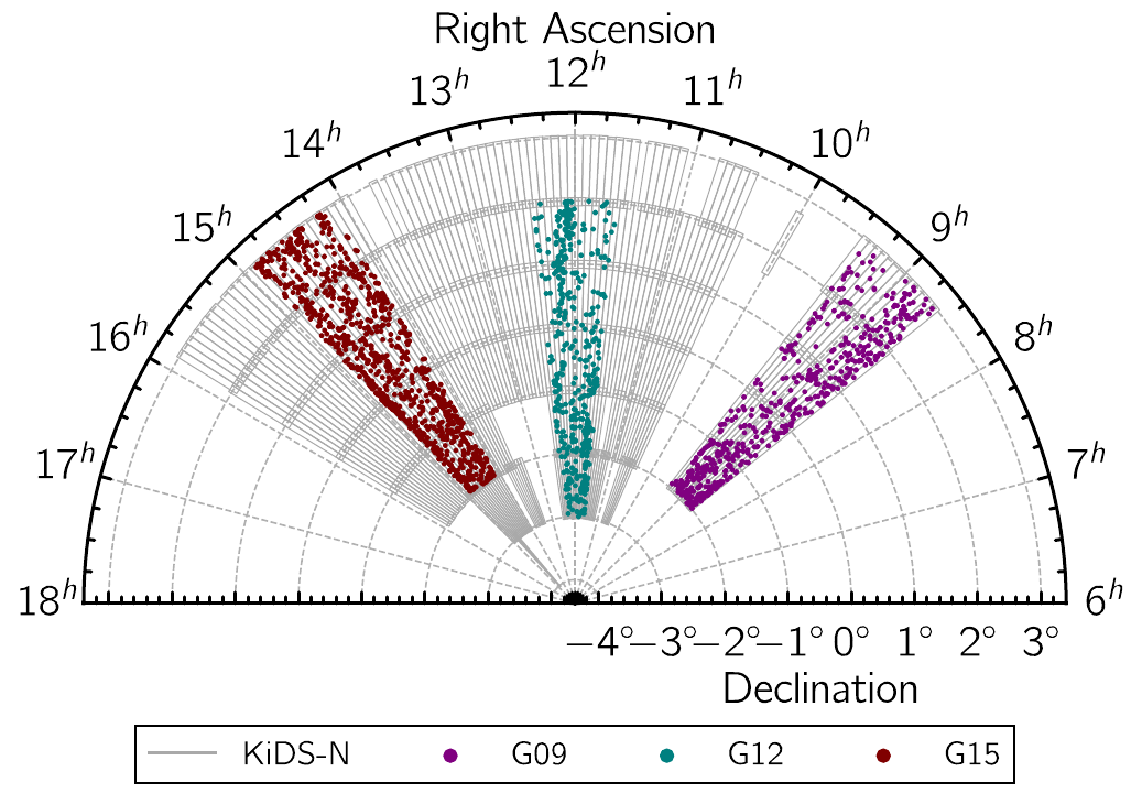
Our galaxy sample was constructed using data from the Galaxy and Mass Assembly (GAMA; Baldry et al. 2018) survey, a large catalogue of galaxies with reliable redshifts obtained from spectroscopic and multi-wavelength observations. The Anglo-Australian Telescope’s (AAT) AAOmega multi-object spectrograph was used to conduct the survey, which covered three equatorial (G$09$, G$12$ and G$15$) and two southern regions (G$02$ and G$23$). The first three, chosen for this study, each encompassed $\sim 5\mathrm{°}$ in declination and $\sim 12\mathrm{°}$ in right ascension, and were centred at roughly $9\text{\,}\mathrm{\textsuperscript{h}}$ (G$09$), $12\text{\,}\mathrm{\textsuperscript{h}}$ (G$12$) and $15\text{\,}\mathrm{\textsuperscript{h}}$ (G$15$). Fig. 1 shows the locations of galaxies from regions G$09$, G$12$ and G$15$ in relation to tiles from KiDS-N, revealing that practically all of these galaxies are included within the KiDS footprint. This makes it straightforward to match GAMA galaxies to KiDS tiles and create cutouts centred on any individual galaxy. Our

Figure 3: Composite $g,r,i$ idealized synthetic images from the simulated TNG50 sample, as obtained with the process described in Section 2.4. Realistic $r$-band counterparts are shown in the first three rows of Fig. 4. Labels denote the stellar mass of each galaxy.

Figure 4: First three rows: $r$-band synthetic images of TNG50 galaxies after applying realism (convolution with a PSF and addition of shot and background noise) to the underlying idealized images, as described in Section 2.4, with the labels indicating the corresponding stellar masses. Last three rows: GAMA-KiDS $r$-band galaxy images with upper (lower) labels indicating their redshift (stellar mass).

position matching approach yields a sample of $104~{}993$ objects with KiDS imaging from an initial sample of $105~{}474$ GAMA galaxies.

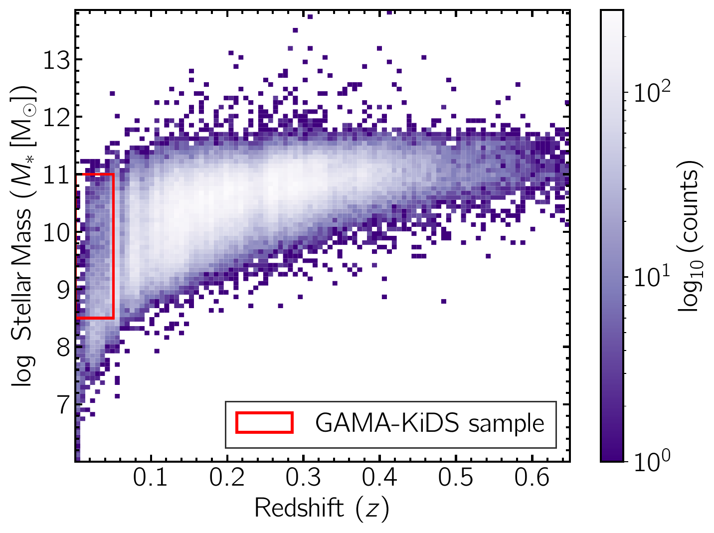
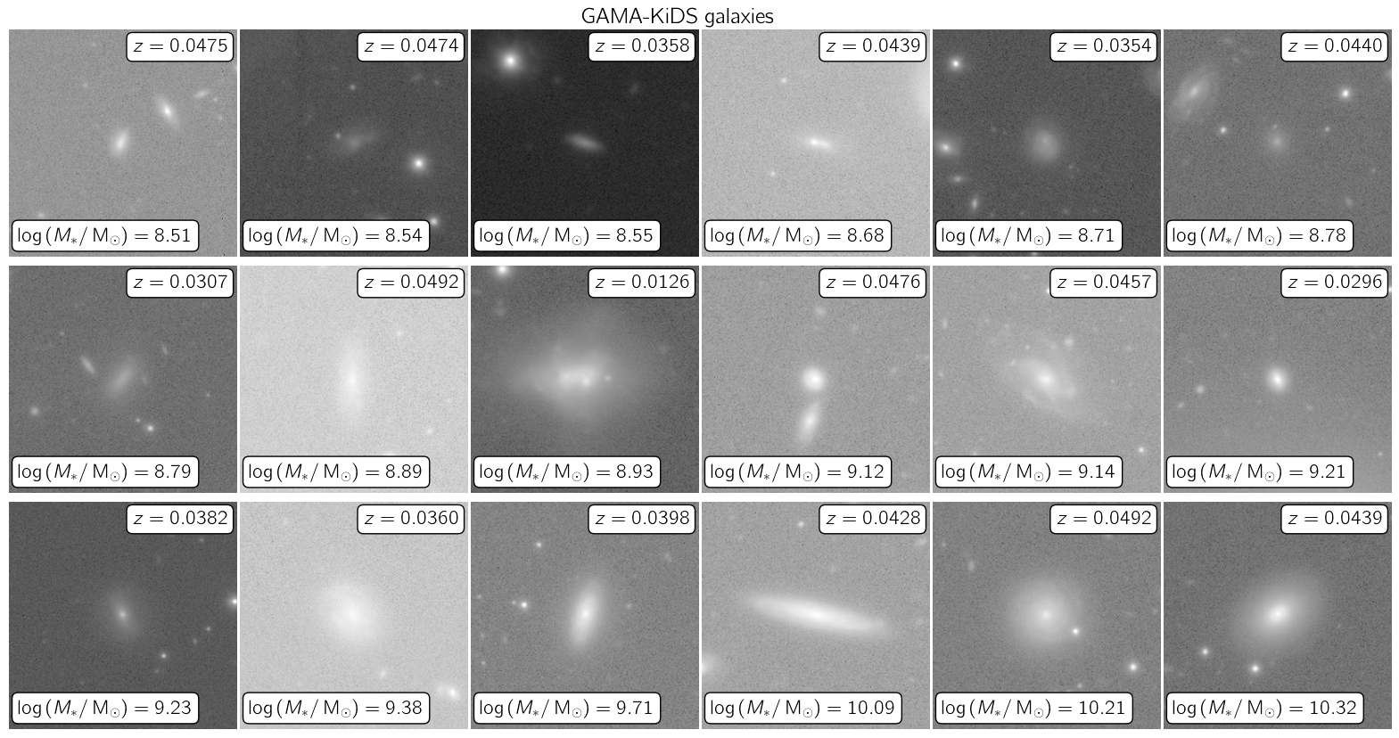
From GAMA’s third data release (Baldry et al., 2018) we use the StellarMasses (Taylor et al., 2011) and SpecCat (Liske et al., 2015) products to obtain the stellar mass, redshift and location (right ascension and declination) for the examined galaxies. The distribution of stellar masses and redshifts of GAMA galaxies can be seen in Fig. 2. For this study, we selected galaxies in the mass range $8.5\leqslant\log\quantity(M_{\ast}/\mathrm{M}_{\odot})\leqslant 11$ with redshift $z<0.05$ in order to perform a direct comparison to a single snapshot from the TNG$50$ simulation. Our final GAMA-KiDS sample consisted of $1238$ objects, and is illustrated in both Figures 1 and 2.

Finally, having defined our galaxy sample based on the GAMA catalogues, KiDS cutouts for individual galaxies were created using utilities from the astropy library (Robitaille et al., 2013; Price-Whelan et al., 2018). Specifically, the function match_coordinates_sky was used to locate the nearest KiDS tile that contained a given GAMA galaxy. Then, the function Cutout2D was employed to create individual images with a fixed size of $240\times 240$ pixels. Overall, $104~{}993$ cutouts were obtained from this matching procedure.

2.3 Simulated sample

We consider galaxies from the TNG50 simulation with stellar masses in the range $8.5\leqslant\log(M_{\ast}/\text{M}_{\odot})\leqslant 11$, which is consistent with our GAMA-KiDS sample, from a single simulation snapshot at $z=0.034$ (snapshot $96$) that is close to the median redshift of the galaxies in our observational sample. The resulting mock galaxy catalogue consists of $5561$ galaxies.

Figure 5: Segmentation procedure. Leftmost panel: real KiDS $r$-band image showing multiple sources; second from left: segmentation map obtained from the previous image; second from right: regularised segmentation map for the object of interest (central galaxy); rightmost entry: regularised mask.

2.4 Synthetic image generation

Galaxy images were constructed from the light distributions of stellar populations, including dust effects such as scattering and attenuation. Following Rodriguez-Gomez et al. (2019), we use different image generation pipelines based on the value of the star-forming gas fraction ($f_{\mathrm{gas,\,sf}}$) in simulated galaxies: synthetic images for galaxies with $f_{\mathrm{gas,\,sf}}<0.01$ were generated using the galaxev stellar population synthesis code (Bruzual & Charlot, 2003), while galaxies with $f_{\mathrm{gas,\,sf}}\geqslant 0.01$ additionally model young stellar populations (age $<$ 10 Myr) with the mappings-iii libraries (Groves et al., 2008) and include dust radiative transfer using the skirt code (Baes et al., 2011; Camps & Baes, 2015). We note that we avoid processing low-gas galaxies with skirt simply for performance reasons, and that both pipelines would produce essentially indistinguishable images for such objects (further details can be consulted in Rodriguez-Gomez et al. 2019).

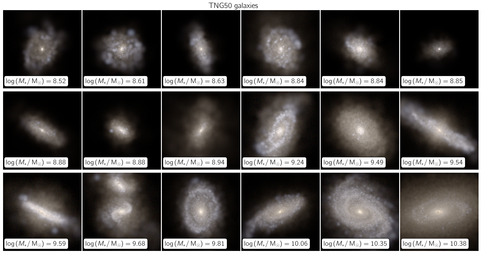
For both pipelines, the light contribution from each stellar particle was smoothed using a particle hydrodynamics spline kernel (Hernquist & Katz, 1989; Springel et al., 2001a) with an adaptive smoothing scale given, for each simulation particle, as the three-dimensional distance to the $32$nd nearest neighbour. Furthermore, the synthetic images were created with the pixel scale of KiDS ($0.2\text{\,}\mathrm{arcsec}\text{\,}{\mathrm{pixel}}^{-1}$) and were mock-observed from the Cartesian projections xy, yz and zx, also setting the field of view of each object to $240\times 240$ pixels, and taking cosmological effects into account (such as surface brightness dimming) assuming they are located at $z=0.034$. This procedure yielded idealised images in four broadband filters corresponding to the $g,r,i,z$ bands, of which we exclusively used the $r$-band for our analysis. We point out that galaxies from the $xy$ projection were used in the discussion presented in Sections 3.1 and 3.2, while galaxies from all three projections were employed from Section 3.3 onwards. The units of the synthetic images are analog-to-digital units (ADU) per second, consistent with real KiDS science images. Fig. 3 shows composite images of randomly selected galaxies from the simulated sample, presented in order of increasing stellar mass, using the KiDS $g,r,i$ filters.

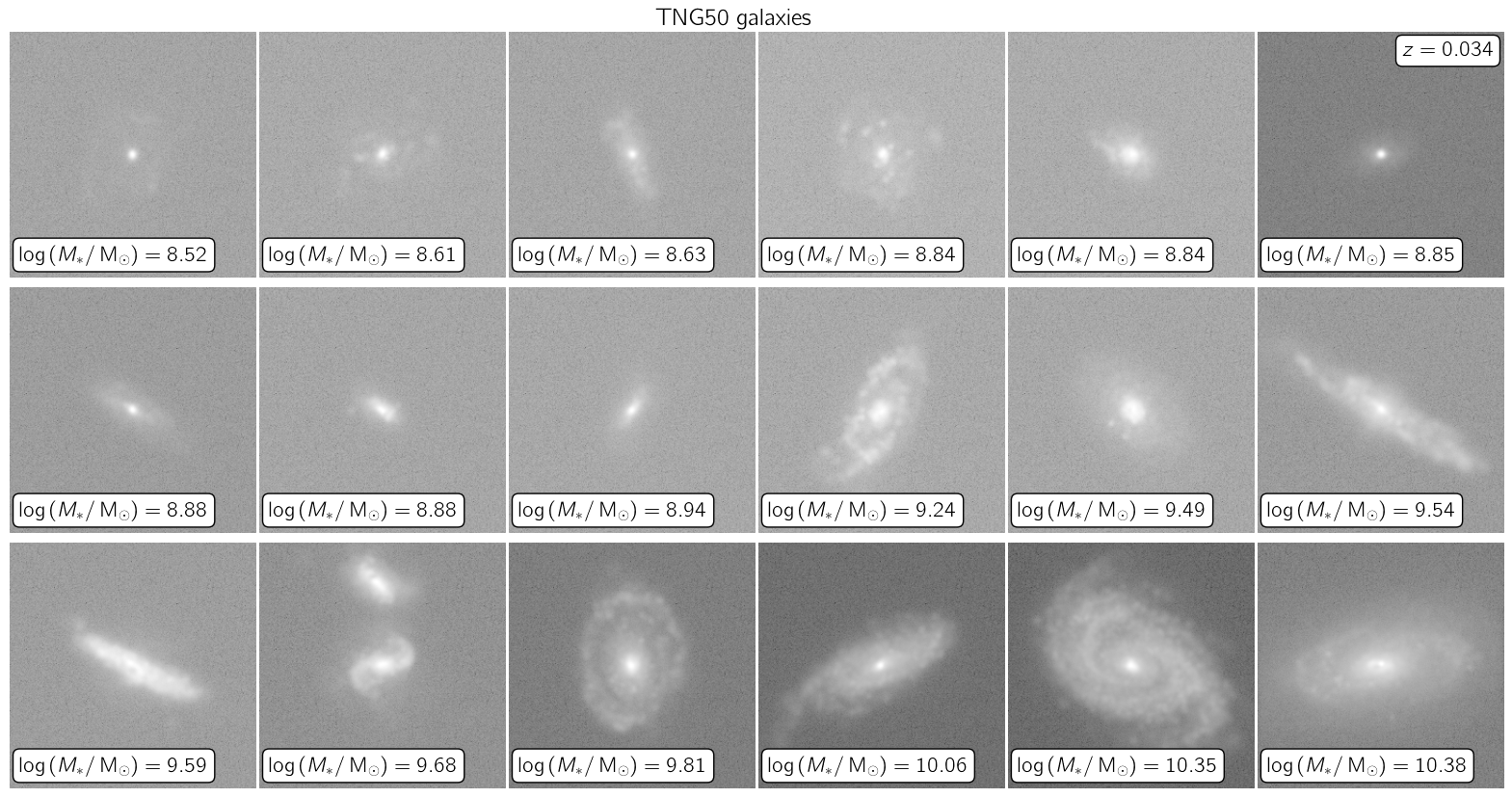
Finally, realism was added to the idealised images via convolution with a point spread function (PSF) and addition of shot and uniform background noise. We convolved each image with a 2D Gaussian PSF with full width at half maximum (FWHM) equal to $0.\mathrm{″}7$, which corresponds to the median PSF from KiDS $r$-band images. Shot noise was included by assuming an effective gain of $3\times 10^{13}$ electrons per data unit, also consistent with KiDS data products, while background noise was modelled as a Gaussian random variable with uniform standard deviation $\sigma_{\mathrm{bkg}}=2\times 10^{-12}\,\mathrm{ADU\,s^{-1}}$ across each simulated image. The first three rows from Fig. 4 show the same synthetic images of Fig. 3 after adding realism, which are compared in the next three rows to randomly selected galaxies from observations.

Table 1: Galaxy deblending and segmentation parameters used by sep.

Parameter	Description	Value
minarea	Minimum galaxy area	10 pixels
deblend_nthresh	Number of deblending levels	16
deblend_cont	Minimum deblending contrast	0.0001
thresh	Minimum detection threshold	0.75

2.5 Source segmentation and deblending

Segmentation is the process in which distinct sources within an astronomical image are labelled with different integer values, reserving the zero-value for the background. The resulting array, with the same shape as the original image, is called a segmentation map or segmentation image.

Proper segmentation is a crucial step for the morphological measurements presented in Section 2.6, since it defines the region that corresponds to the galaxy of interest while removing contaminant objects. The most challenging stage of this procedure is deblending, i.e. the separation of two or more overlapping different sources.

Since we are interested in morphology-based merger identifications on individual galaxies (instead of, for example, counting close pairs) and because it is almost impossible, based on imaging alone, to distinguish between true companions and contaminants (such as chance projections along the line of sight), deblending was applied to all examined sources.

Thus, we have created segmentation maps for both the observational and mock samples using sep (Barbary, 2016), a Python library that implements the core functionality of SExtractor (Bertin & Arnouts, 1996). We have controlled source detection and deblending using the following sep input parameters: thresh, the detection threshold in standard deviations; minarea, the minimum number of pixels in an object; deblend_nthresh, the number of deblending levels, and deblend_cont, the minimum contrast ratio for source deblending. The values of these input parameters are given in Table 1.

Based on segmentation maps, we produced a mask for each galaxy. This was accomplished by identifying the object that coincided with the galaxy of interest and labelling it as the main source; the remainder of the segments, excluding the background, constituted the mask. It is worth mentioning that the main segment and the mask were regularised in the sense that they were smoothed by a uniform filter with a size of $10\times 10$ pixels. Fig. 5 shows a schematic of this procedure.

2.6 Morphological measurements

Morphology calculations were done using statmorph (Rodriguez-Gomez et al., 2019), a Python package for computing non-parametric morphological diagnostics of galaxy images, as well as fitting 2D Sérsic profiles. In order to run the code we used the science images, their segmentation maps and their associated masks, as well as the gain factor, a scalar that converts the image units into $e^{-}\,\text{pixel}^{-1}$, using the same value as in Section 2.4.

In this work we consider the following parameters: concentration, asymmetry and smoothness (CAS; Conselice, 2003), Gini-$M_{20}$ statistics (Lotz et al., 2004; Snyder et al., 2015a; Snyder et al., 2015b), multimode, intensity and deviation (MID; Freeman et al., 2013) and variations of the asymmetry parameter, such as the outer ($A_{O}$; Wen et al., 2014) and shape ($A_{S}$; Pawlik et al., 2016) asymmetries. Below we briefly describe each of them.

The concentration parameter ($C$; Bershady et al. 2000; Conselice 2003) is a measure of the quantity of light at a galaxy’s centre in comparison to its outskirts and is given by $5\log(r_{80}/r_{20})$, where $r_{20}$ and $r_{80}$ are the radii of circular apertures containing 20% ($r_{20}$) and 80% ($r_{80}$) of the galaxy’s total flux. Elliptical galaxies exhibit high concentration ($\sim 4$) values, whereas spiral galaxies have smaller ($\sim 3$) values.

The asymmetry index ($A$; Abraham et al. 1996; Conselice et al. 2000; Conselice 2003) is calculated by subtracting a galaxy image from its ${180}^{\circ}$-rotated counterpart, and is used as a measure of what fraction of light is due to non-symmetric components. The equation for computing this parameter is given by

$$A=\frac{\sum_{i,\,j}\absolutevalue{I_{ij}-I_{ij}^{180}}}{\sum_{i,\,j}\absolutevalue{I_{ij}}}-A_{\textsc{bkg}},$$ (1)

where $I_{ij}$ and ${I}_{ij}^{180}$ are, respectively, the pixel flux values of the original and rotated distributions, and $A_{\textsc{bkg}}$ is the average asymmetry of the background. High asymmetry values are often used to identify possible recent interactions and galaxy mergers.

Combination	Parameter
	$C$	$A$	$S$	$F\quantity(G,\,M_{20})$	$S\quantity(G,\,M_{20})$	$M$	$I$	$D$	$A_{O}$	$A_{S}$
1	Yes	Yes	Yes	Yes	Yes	No	No	No	No	No
2	Yes	Yes	Yes	Yes	Yes	Yes	Yes	Yes	No	No
3	No	Yes	Yes	No	No	No	No	No	Yes	Yes

Table 2: Feature combinations considered during hyper-parameter tuning and cross-validation.

The smoothness parameter ($S$; Conselice 2003) is estimated in a similar way to the asymmetry, by subtracting a galaxy distribution from a counterpart that has been smoothed by a boxcar filter of width $\sigma$, and it indicates the fraction of light that is contained in clumpy regions (e.g. high frequency disturbances). Following Lotz et al. (2004), we set the value of $\sigma$ to $25\%$ of the Petrosian radius.

The Gini index ($G$; Abraham et al. 2003; Lotz et al. 2004) quantifies the degree of inequality of the brightness distribution in a set of pixels. The Gini coefficient is equal to $1$ when all the galaxy light is concentrated in one pixel; conversely, it is equal to zero when the light distribution is homogeneous across all pixels. Early-type galaxies, as well as galaxies with one or more bright nuclei, exhibit high Gini values.

The $M_{\mathrm{20}}$ coefficient is the normalised second moment of a galaxy’s brightest regions, containing $20\%$ of the total flux. Mergers and star-forming disk galaxies tend to have high $M_{20}$ values.

The bulge parameter ($F(G,\,M_{20})$; Snyder et al. 2015b) is a linear combination of $G$ and $M_{\mathrm{20}}$. In the $G$-$M_{\mathrm{20}}$ space, early-type, late-type and merging galaxies are found by the position they occupy relative to two intersecting lines (Lotz et al., 2008). The bulge parameter, $F(G,\,M_{20})$, is then defined as the position along the line with origin at the intersection $\quantity(G_{0}=0.565,M_{20,\,0}=-1.679)$ that is perpendicular to the line that separates early-type and late-type galaxies, scaled by a factor of $5$,

$$F\quantity(G,\,M_{20})=-0.693M_{20}+4.95G-3.96.$$ (2)

The merger parameter ($S(G,\,M_{20})$, Snyder et al. 2015a) has a similar definition to $F\quantity(G,\,M_{20})$. It is given as the position along a line with origin at $\quantity(G_{0},M_{20,\,0})$ that is perpendicular to the line that separates mergers from non-mergers,

$$S\quantity(G,\,M_{20})=0.139M_{20}+0.990G-0.327.$$ (3)

The multimode ($M$; Freeman et al. 2013) parameter is the pixel ratio of the two brightest regions of a galaxy, which are identified following a threshold method: bright regions are identified when they are above a threshold value, a process repeated for different values until the ratio is the largest. Double-nuclei systems tend to have values close to one.

The intensity ($I$; Freeman et al. 2013) parameter is the flux ratio between the two brightest subregions of a galaxy. For its computation the watershed algorithm is used, i.e. the galaxy image is divided into groups such that each subregion consists of all pixels whose maximum gradient paths lead to the same local maximum. Clumpy systems often exhibit high intensity values.

The deviation ($D$; Freeman et al. 2013) parameter is given as the normalised distance between the image centroid and the centre of the brightest region found during the computation of the $I$-statistic, and is used to quantify the offset between bright regions of a galaxy and the centroid.

The outer asymmetry ($A_{O}$; Wen et al. 2014) parameter is defined in the same way as the conventional asymmetry (see eq. 1), with the exception that pixels from the inner elliptical aperture that contains $50\%$ of the galaxy’s light are not included in the computation. Pixels outside this area build up the outer half-flux region, for which $A_{O}$ is estimated. Lastly, the shape asymmetry ($A_{S}$; Pawlik et al. 2016) parameter is also calculated in the same way as the standard asymmetry, with the difference that the measurement is done over a binary segmentation map rather than the galaxy brightness distribution.

Finally, statmorph provides a flag quality parameter to distinguish between reliable and unsuccessful measurements, which are labelled with flag == 0 and flag == 1, respectively. We find that the overall fraction of flagged galaxies is low, representing ${\lesssim}10\%$ for both our observational and simulated samples. From this point onwards we only consider galaxies with reliable morphological measurements, also imposing, for each object, a minimum signal-to-noise ratio $\expectationvalue{S/N}\geqslant 2.5$.

2.7 Merger identification

Galaxy mergers in the TNG50 simulation can be identified using merger trees created using the sublink code (Rodriguez-Gomez et al., 2015). The idea behind the merger trees is to associate a given subhalo with its progenitors and descendants from adjacent snapshots, in such a way that a merger event occurs when a subhalo has two or more different progenitors. From the merging history catalogues of the TNG50 simulation, we have determined which galaxies from our synthetic sample have experienced a merger within a given period.

The merger mass ratio is defined as $\mu=M_{2}/M_{1}$, where $M_{1}$ and $M_{2}$ are the stellar masses of the primary and secondary progenitors, respectively, measured at the moment when the secondary progenitor reaches its maximum stellar mass (Rodriguez-Gomez et al., 2015). Traditionally, major and minor mergers are defined as those with $\mu>1/4$ and $1/10<\mu<1/4$, respectively. Throughout this paper we consider a combined sample of major + minor mergers, with mass ratios $\mu>1/10$, for all our computations. The main reason for this choice is to have a larger training sample for our classifier, but it also has the advantage of potentially detecting merger signatures that are more subtle or long-lasting than those produced by major mergers. As discussed in Lotz et al. (2011), both the Gini–$M_{20}$ statistics and the asymmetry parameter are sensitive to minor mergers as well as major ones.

In this context, our intrinsic merger sample is composed of mergers that occurred within ${\pm}0.5$ Gyr relative to the reference redshift ($z=0.034$; snapshot 96). For definiteness, we note that this time window includes mergers that were recorded in the snapshots 94 to 99 (since for a merger event recorded at snapshot $k$, the merger must have actually taken place at some time between snapshots $k-1$ and $k$), and represents an observability time-scale of $\approx 1$ Gyr. From a sample of 15 463 galaxy images with successful morphological measurements, we identified 833 major + minor mergers within the specified time window, representing an overall merger fraction of about 5%.

2.8 Random forest classification

The random forest (RF) algorithm (Breiman, 2001) is an ensemble method based on independent decision trees, each of them learning from subsamples of the input data. Predictions on unseen data are then given as a majority vote among all uncorrelated models given by the trees in the forest. The goal of the algorithm is to learn a rule from the galaxy inputs $\mathbf{x}$ (morphological measurements) to the labels $y$ (merger statistics), and then generalise over novel inputs.

In this study, feature space is defined by the CAS, Gini-$M_{20}$, MID, $A_{O}$ and $A_{S}$ parameters, representing a total of 10 features, with inputs given as values of these attributes for the galaxies. In other words, inputs can be seen as vectors $\mathbf{x}_{i}$ having different morphological values in each entry. Likewise, the target values of the algorithm are given by the merger label $y_{i}$ of each galaxy, with $y_{i}=1$ if the given input is a true intrinsic merger (as defined in Section 2.7), and $y_{i}=0$ otherwise.

The scikit-learn module (Pedregosa et al., 2011) was used to construct random forests. The library’s internal implementation of the classifier is based on the algorithm of Breiman (2001), which incorporates bootstrapping of the training set and randomised feature selection. Utilities from this and the imbalanced-learn library (Lemaître et al., 2017) were also used. The receiver operating characteristic (ROC) curve was considered to assess the performance of each model.

In this sense, positive predictive value (PPV, also known as purity or precision) is the ratio between the true positives (TP; true mergers selected by the classifier) and the sum of all objects selected, which are the false positives (FP; non-mergers selected by the classification) and true positives, that is, $\text{PPV}=\text{TP}/(\text{TP}+\text{FP}).$ Similarly, true positive rate (TPR, also known as completeness or recall) is the ratio between TP and the total number of intrinsic mergers, which is the sum of true positives and false negatives (FN; true mergers rejected by the classifier), i.e. $\mathbf{\text{TPR}=\text{TP}/(\text{TP}+\text{FN}).}$ The ROC curve is a plot of the TPR against the false positive rate (FPR) at various threshold values, where the latter is computed as the ratio of FP and the total number of intrinsic non-mergers, which in turn are given as the sum of FP and true negatives (TN; non-mergers rejected by the algorithm): $\text{FPR}=\text{FP}/(\text{FP}+\text{TN})$. The ROC curve of a random classifier (with no predictive power) is a diagonal line from the origin to the point $(1,1)$ whereas a perfect classifier is described by two lines, the first of these starting from the origin to $(0,1)$ and the second one from $(0,1)$ to $(1,1)$, so that it has $\text{TPR}=1$ and $\text{FPR}=0$.

Our full learning dataset consists of 15 463 inputs corresponding to successful morphological measurements performed on synthetic galaxy images in three orientations along the axes of the simulation volume, each of them having different values, along with their corresponding merger labels (ground truth).

We split our full dataset into training and test sets, assigning $70\%$ of the inputs to the first set, and the remaining $30\%$ to the second set. This division was done in a stratified manner, which keeps the original proportion of distinct classes (merger or non-merger) in both samples. We point out that in the full dataset there are ${\sim}18$ non-mergers for each merger. Thus, class imbalance was offset by randomly under-sampling (RUS) the majority class (non-mergers) to bring it to the same size as the merger set. This method is implemented in the imbalanced-learn library, and was applied before fitting the random forest. We also tried over-sampling the minority class (mergers) using the Synthetic Minority Over-sampling Technique (SMOTE, Chawla et al. 2002), which resulted in approximately the same performance. Therefore, from this point onwards we will only show results obtained with the RUS technique.

Similarly, the tuning of hyperparameters (i.e. parameters used to control the training process, instead of those derived from it) was done by means of cross-validation on the training set, conducting a 5-fold stratified scheme. This entails randomly dividing the training set into five folds, retaining the proportion of mergers and non-mergers, and repeatedly training the classifier with a combination of four of these samples while validating (testing) the remaining one. Cycling over all splits, the random forest classifier is trained and validated on five different subsets of the original training set. Simultaneously, the hyper-parameters of each forest can be optimised in a grid search fashion. In this step the main optimised parameters were the number of trees in the forest, the depth of each tree, the maximum number of leaf (terminal) nodes, and the balancing of the sample. Accordingly, we used, respectively, the RandomForestClassifier function from scikit-learn to tune the n_estimators, max_depth, max_leaf_nodes and class_weight parameters, while keeping the rest of hyper-parameters at their default values.

Furthermore, during training we have explored several combinations and sub-samples from all morphological attributes in order to test how well they would perform on their own. Table 2 shows all such combinations considered in the RF models. Lastly, the entire procedure was carried out with the pipeline and GridSearchCV functions from the scikit-learn and imbalanced-learn libraries, which allow for cross-validation and exhaustive hyper-parameter tuning at the same time. The end result of the process is a trained model and a combination of hyper-parameters that give, according to a particular metric, the ’best’ classification of the data. Additionally, the classifier provides for each of the galaxies considered, a probability score that is used to label them (as mergers or non-mergers). As such, this threshold can be varied in order to reach a compromise between successful and unsuccessful classifications. This is usually done by maximising certain metrics, such as the $F_{1}$-score or the Matthews correlation coefficient , or by computing the balance point, namely the point for which $\mathrm{TPR=1-FPR}$. In this work we use the latter approach as the default probability threshold, emphasizing that we compared this value to those computed with the $F_{1}$-score and the Matthews coefficient, finding similar results between these thresholds and the balance point, which in turn mean that there are no significant differences for the performance metrics that we present in Section 3.3.

Figure 6: Pairwise plots of $r$-band morphological parameters from the observational GAMA-KiDS (blue) and simulated TNG50 (red) samples, with univariate distributions shown on the diagonal. The bi-dimensional kernel density estimates are shown with contours at $\{0.1,0.2,0.5,0.8,0.95\}$. This plot indicates that there is good overall agreement between the morphologies of these samples.

Figure 7: Median trends as a function of stellar mass for several $r$-band morphological parameters. The solid red and blue lines indicate the simulated (SKIRT pipeline) and observational results, respectively; the dashed line corresponds to synthetic images generated without the effects of a dust distribution (GALAXEV pipeline). This figure again shows that there is good agreement between theory and observations, with the median values (at fixed stellar mass) of all morphological parameters in TNG50 lying within 1$\sigma$ of the observational trends; it also shows that the simulated galaxies are more concentrated and asymmetric than their observational counterparts.

Figure 8: Pairwise distributions of $r$-band morphological parameters for the non-merging population (black) against the distributions of mergers (green), with contours located at $\{0.05,0.1,0.2,0.5,0.8,0.95\}$. This figure demonstrates that simulated merging and non-merging systems exhibit a high degree of overlap in their morphologies, occupying similar regions in parameter space; it also indicates that the distributions of the merging population tend to have higher distribution values, which is more noticeable for the asymmetry parameter.

Figure 9: Median trends as a function of stellar mass for several $r$-band morphological parameters. The solid black and green lines indicate the low-mass non-merging and merging TNG50 galaxy populations, respectively. Although merging systems tend to be more asymmetric at all stellar masses, this plot shows that the morphologies of these two samples are highly comparable, particularly at the low mass end.

Figure 10: Top row: ROC curves for random forest models trained on the full dataset using the combinations in listed in Table 2; asymmetry and merger statistic lines indicate merger selections using only one of these parameters. The hexagons, triangles and circles indicate default threshold values for the classifier (balance point), asymmetry parameter ($0.25$) and merger statistic ($0.0$) selections. Bottom row: feature importance for each model corresponding to the random forest ROC curves above. The vertical axis indicates the name of the corresponding attributes, while the horizontal axis denotes the percentage, i.e., the parameters’ contribution to classification decisions. In all cases the asymmetry or outer asymmetry parameters had the highest weight on decisions, with the merger statistic, smoothness or asymmetry parameter (combination 3) ranking second in their respective combination.

3 Results

3.1 The morphologies of TNG50 and GAMA-KiDS galaxies

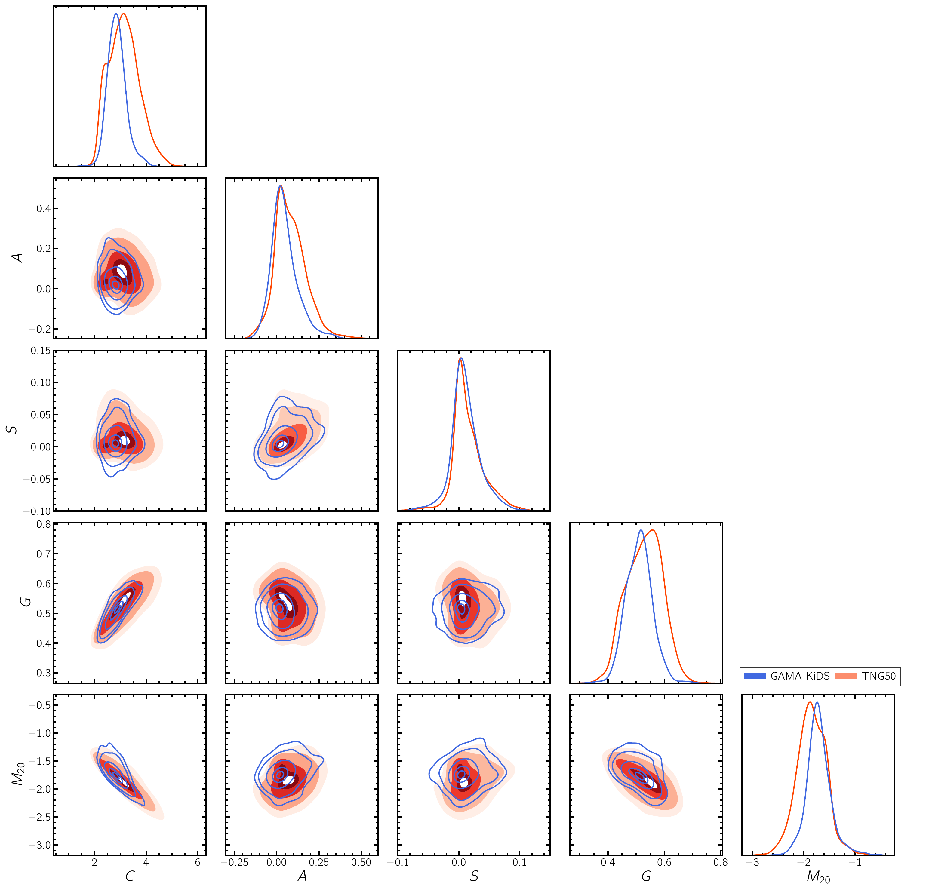
Fig. 6 shows pairwise plots of various morphological parameters measured by statmorph for our simulated (TNG50, red shaded regions) and observational (KiDS, blue contours) galaxy samples. In the former case, we only show measurements for a single projection (onto the $xy$-plane). The plots in the lower triangle of Fig. 6 show the joint distributions of the various morphological parameters, while the plots on the diagonal show their univariate distributions. As can be seen, there is reasonable agreement between the morphologies of simulated galaxies and those of the real observational sample. However, Fig. 6 also reveals some differences between the two samples. For instance, the concentrations and Gini coefficients of TNG50 galaxies peak at slightly higher values than their observational counterparts, while the distribution of the $M_{20}$ parameter reaches a maximum at a slightly lower value. These trends indicate that TNG50 galaxies tend to be slightly more concentrated objects than real galaxies of similar stellar mass. On the other hand, the asymmetry distribution reaches a peak very close to zero for both samples, but displays a tail toward higher values for TNG50 galaxies, indicating that these objects tend to be slightly more asymmetric than their observational counterparts.

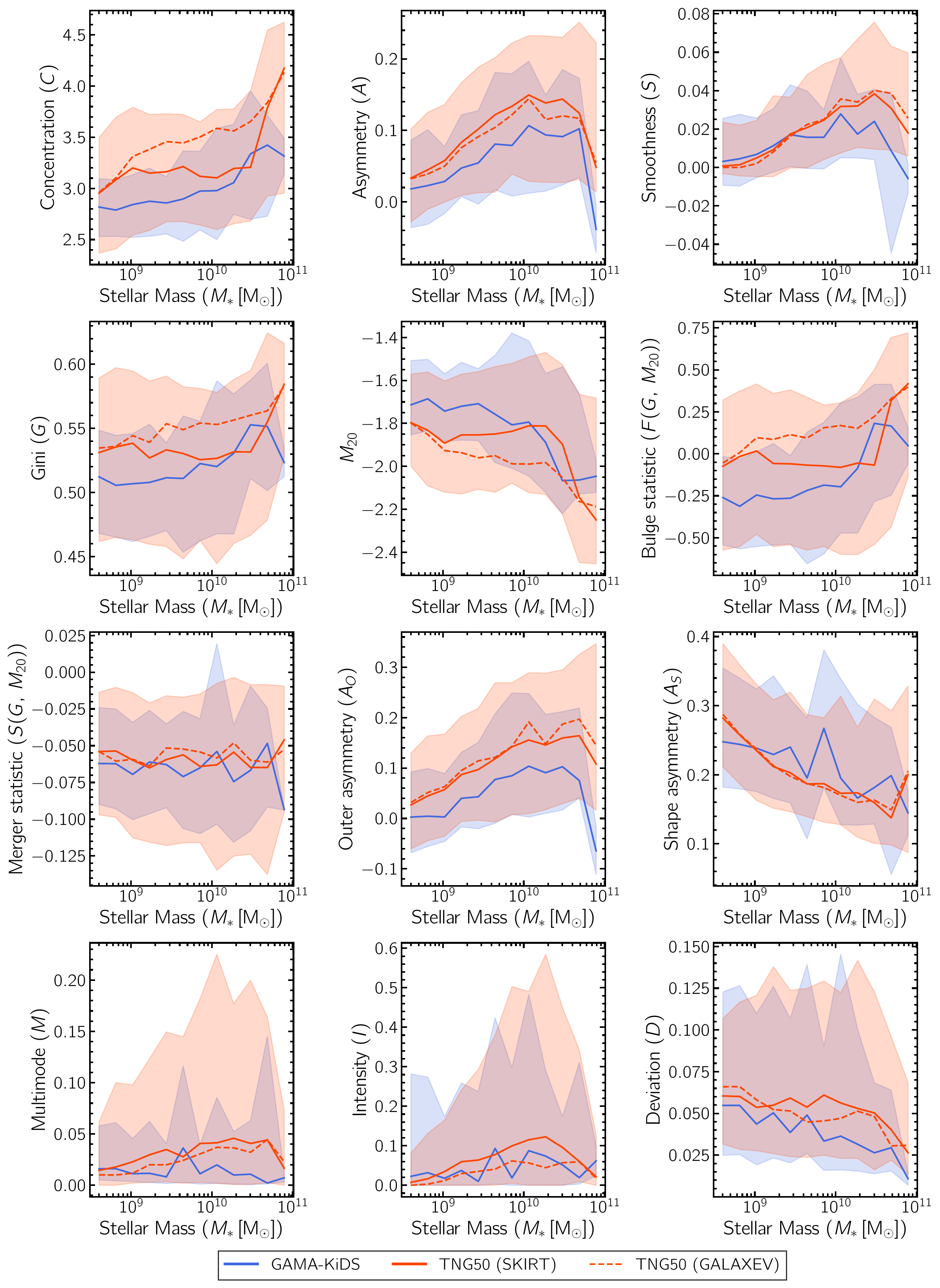
Fig. 7 shows median trends as a function of stellar mass for all morphological parameters considered. The red solid line corresponds to galaxies modelled following our full radiative transfer pipeline, while the dashed one was obtained using simpler models without including the effects of a dust distribution; similarly, the blue solid line indicates the median trend for our GAMA-KiDS sample. The blue and red shaded regions denote the corresponding 16th to 84th percentile range, at a fixed stellar mass, for the observational and simulated (dust effects included) samples, respectively. These figures confirm the overall morphological agreement between observations and simulations: all median trends from TNG50 lie within the $1\sigma$ scatter of the observational measurements. However, closer inspection of Fig. 7 shows again that TNG50 galaxies tend to be slightly more concentrated and asymmetric than their observational counterparts.

Finally, Fig. 7 corroborates that simulated galaxies modelled with dust effects have morphologies better aligned with observations, since dust attenuation tends to reduce the brightness of the central regions, where higher concentrations of gas and dust are typically encountered in the simulation. This effect, however, is not enough to bring the concentrations of low-mass galaxies into full agreement with observations.

3.2 The morphologies of true mergers and non-mergers

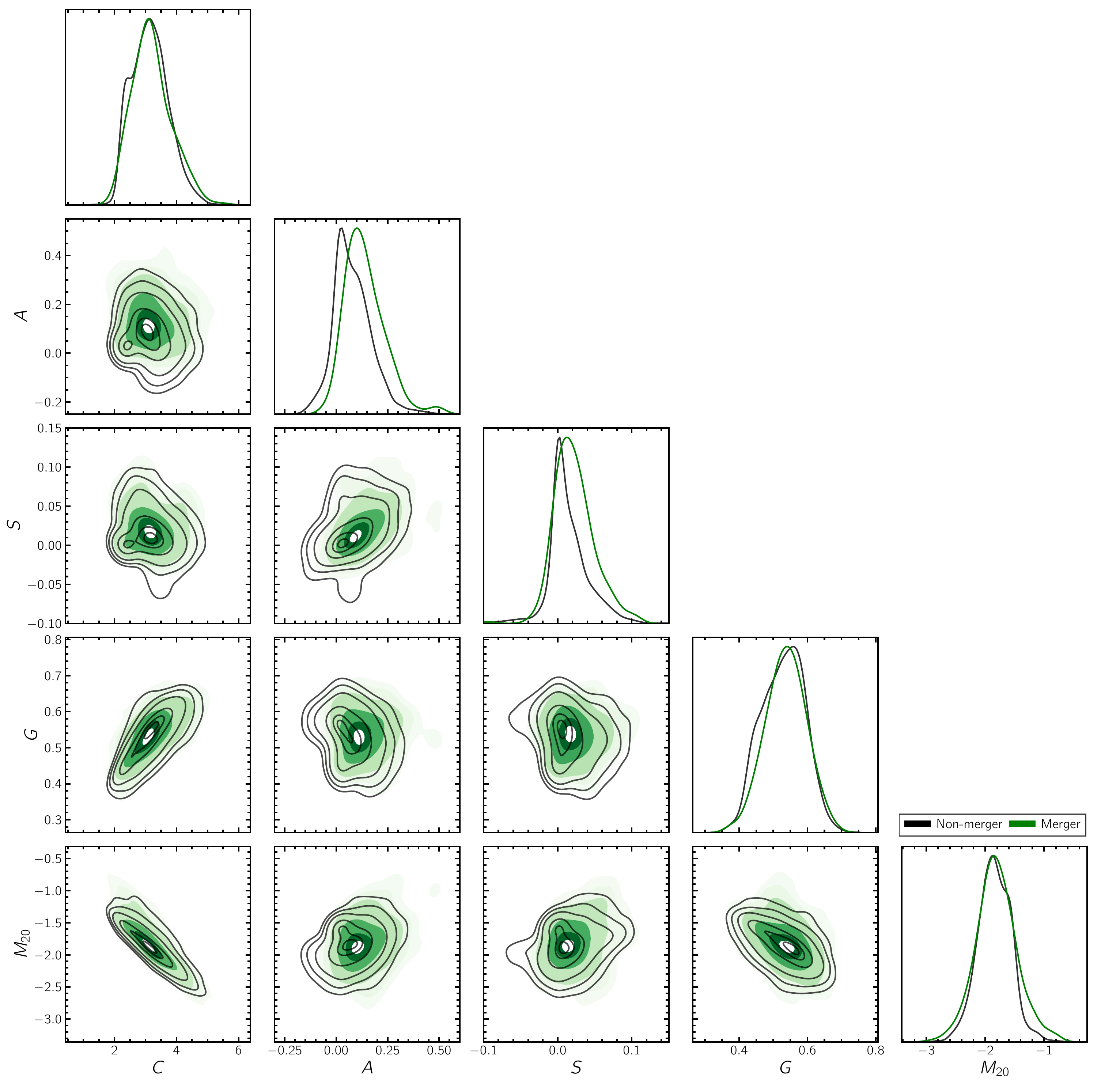
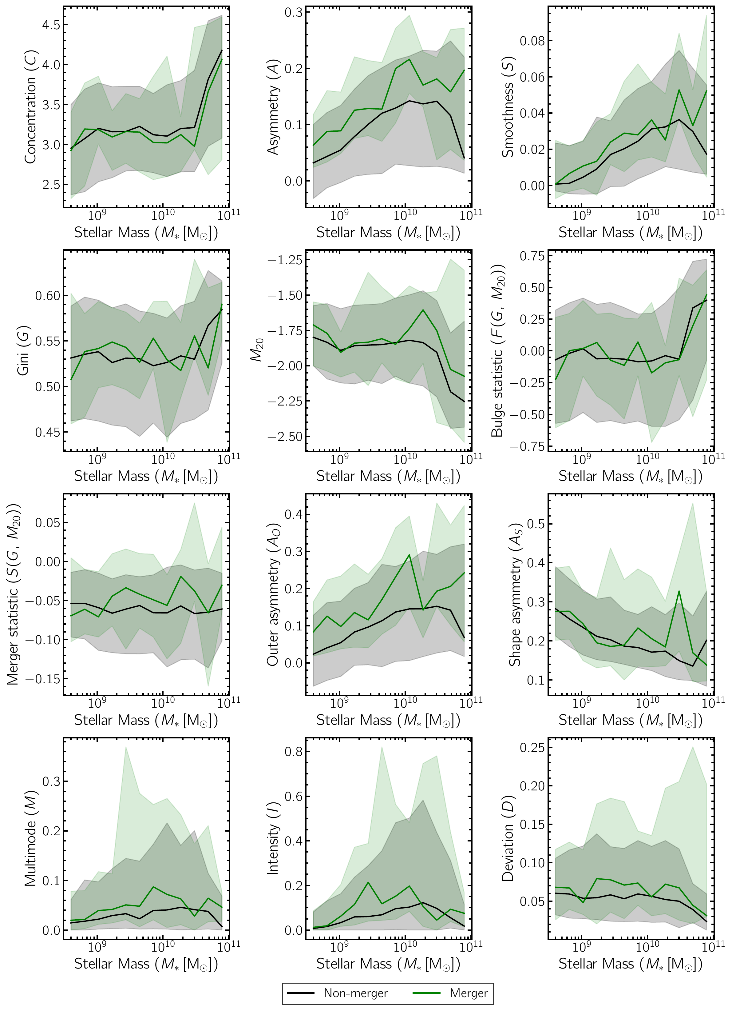
Fig. 8 shows morphology distributions for the merging sample (green shaded regions) defined in Section 2.7 as well as for the non-merging TNG50 population (black contours). As can be seen, the morphologies of these two groups do not differ significantly from each other, i.e. they occupy similar regions in parameter space, as previously pointed out for the case of galaxies at higher redshifts (Snyder et al., 2019). The morphological similarity between mergers and non-mergers can also be seen in Fig. 9, which shows median trends (solid lines) and $1\sigma$ scatter regions (shaded zones) for the relevant morphological parameters as a function of stellar mass. Nevertheless, the asymmetry and outer asymmetry parameters reveal that, although there is significant morphological overlap between mergers and non-mergers, the former are more asymmetric than the latter. In the next sections, we exploit these differences in order to train an image-based galaxy merger classifier.

3.3 Classifying mergers with random forests

3.3.1 Performance and feature importance

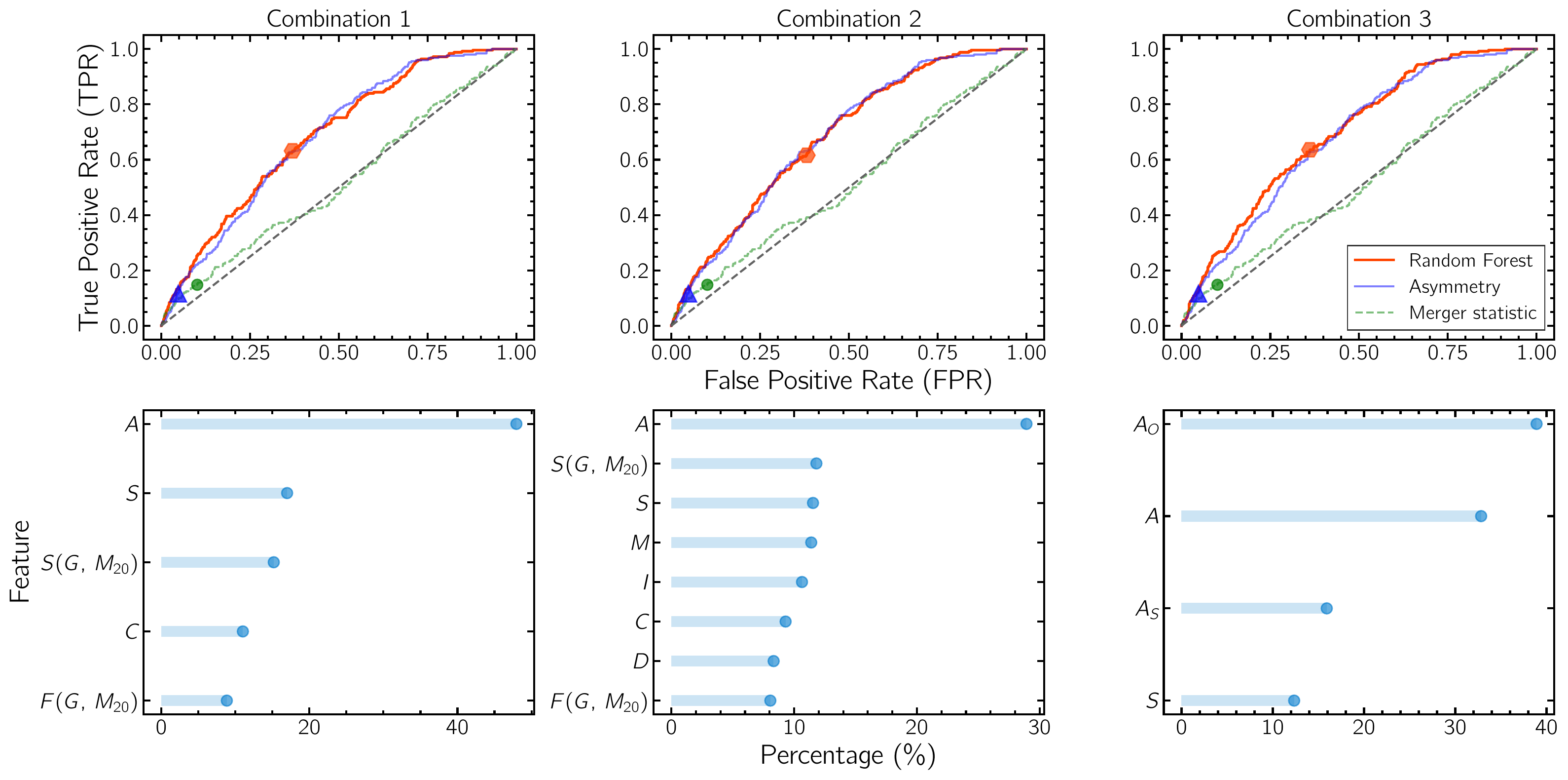
In this section we present results about the merger classification of the mock-catalog as detailed in Section 2.8. The hyper-parameter tuning and cross-validation procedures performed on the training sets result in the best trained models for each of the feature combinations listed in Table 2. Each of these models was then applied to the corresponding test set, which had ${\approx}4389$ non-merging objects and ${\approx}250$ merging galaxies, with stellar masses $8.5\leqslant\log\quantity(M_{\ast}/\mathrm{M}_{\odot})\leqslant 11$. We found that all models yield similar classifications independently of the feature combination used: ${\approx}179$ and $2425$ objects were correctly classified as mergers and non-mergers, respectively; $1964$ non-merging galaxies were misclassified as mergers, and $71$ mergers were misclassified as non-mergers. These findings are translated, for the merger class, into an average purity and completeness of ${\approx}8.4\%$ and ${\approx}72\%$, respectively.

The upper panels of Fig. 10 show the ROC curve (see Section 2.8) for the trained models using combinations 1–3 from Table 2. For reference, we also show the ROC curves that would be obtained by using only the asymmetry parameter or the Gini–$M_{20}$ merger statistic to select merging galaxies. A perfect classifier lies at the upper-left corner and has $\text{TPR}=1$ and $\text{FPR}=0$, while a model that goes in diagonal from $(0,0)$ to $(1,1)$ has no predictive power. Our models have loci between these two regions, with an area under the ROC curve of ${\approx}0.7$, indicating that they are moderately adequate classifiers.

The lower panels of Fig. 10. show, also for the model combinations 1–3, input features and their relative importance to the classification decisions. In this context, feature importance is defined as the mean decrease in impurity achieved by each variable at all relevant nodes in the random forest. In all cases the asymmetry or outer asymmetry parameters had the highest weight ($\sim 30-50\%$) on the classifier decisions, followed in second place by smoothness parameter ($15\%)$ or the merger statistic ($12\%)$. None of the other parameters had a feature importance above 15%.

3.3.2 Default random forest model

The models presented above have similar performance regarding purity and completeness values. These results are consistent with the work by Snyder et al. (2019), who designed random forest models for high-mass galaxies at different redshifts from the original Illustris simulation. For their lowest redshift sample at $z=0.5$, they obtained purity values of up to $10\%$, with completeness at roughly $70\%$. Similarly, the metrics produced by our models are consistent with those found by Bignone et al. (2016) for the Illustris simulation. Specifically, they studied the morphologies of a galaxy sample at $z=0$ with $M_{\ast}>10^{10}\,\text{M}_{\odot}$ and subsequently used the Gini–$M_{20}$ criterion from Lotz et al. (2004) to identify galaxy mergers. Their results, as a function of the time $t$ elapsed since the last merger, show that for $t\sim 1$ Gyr the purity metric is around $5\%$ for cases with $\mu>1/10$ and equal to $9\%$ for $\mu>1/4$. Throughout the rest of this paper we set the RUS+RF model trained with combination one in Table 2 as our default random forest model. This decision is mainly based on the robustness of classification performance for different sets of features, but also because the morphological parameters included in that combination are widely used in the literature (e.g. Lotz et al. 2011, and references therein) to identify both major and minor mergers. In Section 3.4 we use this model to estimate the galaxy merger fraction in the TNG50 simulation, which we compare to the intrinsic merger fraction (i.e. computed with the merger trees), as well as to estimate the galaxy merger fraction in the real Universe by applying our classifier to GAMA-KiDS observations.

Figure 11: Classification result examples made by the random forest model. The upper-left block of figures shows true positives (true mergers selected) while the upper-right block shows true negatives (non-mergers rejected). These objects typically exhibit the expected attributes: true positives (mergers) are perturbed and often have companions, whereas true negatives (non-mergers) tend to be isolated and unperturbed. Similarly, the lower-left block of figures shows false positives (non-mergers selected) while the lower-right part shows false negatives (true mergers rejected). False positives might arise from mergers taking place outside the window detection period or by having similar morphologies to some true mergers; false negatives could emerge from minor mergers failing to trigger morphological disturbances at the time of detection. In all cases the upper text labels indicate the probability value assigned to that object by the random forest, as well as its corresponding asymmetry value.

3.3.3 Classification result examples

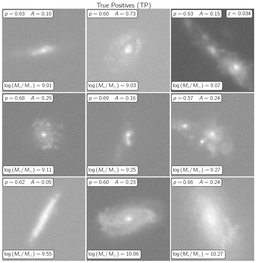
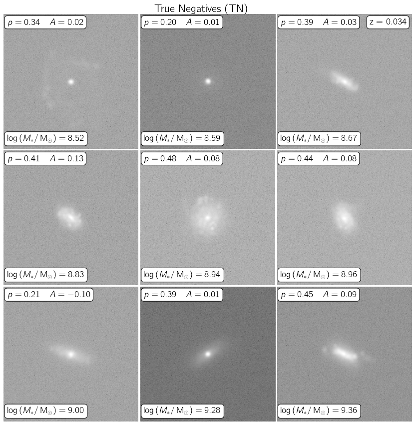
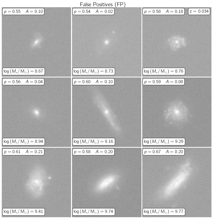
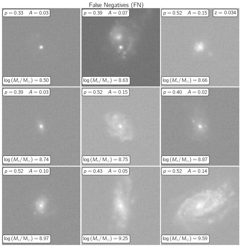
In Fig. 11 we present examples of simulated galaxies that have been classified by our default random forest model and were categorised as true positives and true negatives as well as false positives and false negatives. Note that these objects are sorted in ascending order according to stellar mass. As can be seen in the upper row from Fig. 11, most true mergers exhibit clear signs of interaction, such as asymmetric structures and neighbouring or overlapping companions. Likewise, most non-mergers do not have significantly perturbed morphologies and look relatively isolated. This is particularly noticeable for low-mass objects.

Similarly, the lower row in Fig. 11 shows examples of the failure modes of the classifier. We found that some false positives had relatively asymmetric structures but were not labelled as mergers in our merger tree-based selection (see Section 2.7). Thus, such cases might arise from merging events taking place outside our window detection period or from isolated galaxies that are morphologically similar to mergers (see Figures 8 and 9).

Conversely, some false negatives appear unperturbed so that they are probably the result of minor mergers that did not trigger perceptible morphological signatures. These cases are reminiscent of the findings by Martin et al. (2021), who found that mergers induce limited morphological changes in dwarf galaxies. Thus, the lower part of Fig. 11 illustrates the most common challenges faced by the models. On the one hand, merging events are rare, which reduces the number of class examples and statistics for training; on the other hand, there is a significant degree of similarity between mergers and non-mergers, which explains most of the false positives.

(a)

(b)

Figure 12: (a) Galaxy merger fraction as a function of stellar mass as predicted by our random forest classifier for our simulated and observational galaxy samples, as indicated by the legend. (b) Mass-dependent merger fraction for the observational and simulated galaxy samples as predicted by an asymmetry-based criterion. In both panels, the solid blue line represents the intrinsic merger fraction measured in TNG50 using the merger trees. The error bars represent Poisson uncertainty from the number of mergers in each mass bin. This figure shows that the merger fraction increases steadily as a function of stellar mass for all the approaches considered.

3.4 The merger incidence of GAMA-KiDS observations

We used our default random forest model to estimate the merger fraction in our observational $(z<0.05;8.5\leqslant\log\quantity(M_{\ast}/\mathrm{M}_{\odot})\leqslant 11)$ galaxy sample. The input entries for this model consist of the morphological measurements carried out on the GAMA-KiDS sample (see Section 2.6), corresponding to combination one in Table 2.

Following Snyder et al. (2019), we estimate the merger fraction $f_{\mathrm{merger}}$ as

$$f_{\mathrm{merger}}=\frac{N_{\mathrm{RF}}}{N_{\mathrm{T}}}\frac{\mathrm{PPV}}{\mathrm{TPR}}\expectationvalue{M/N},$$ (4)

where $N_{\mathrm{RF}}$ and $N_{\mathrm{T}}$ are the number of galaxies selected by the forest and the total number of galaxies, respectively; the factor $\expectationvalue{M/N}$ is the average total number of simulated mergers divided by the number of galaxies with at least one such merger, which in our case is approximately equal to one; the term $\mathrm{PPV}/\mathrm{TPR}$ is a corrective factor that takes into account the completeness and purity of the default model, so that when used on novel data the best-guess merger fraction is obtained (Snyder et al., 2019). For comparison, we have determined the intrinsic merger fraction of simulated galaxies by estimating, for each mass bin, the quantity $N_{\mathrm{merger}}/N_{\mathrm{T}}$, where $N_{\mathrm{merger}}$ is the number of intrinsic mergers, obtained from the merger trees as described in Section 2.7.

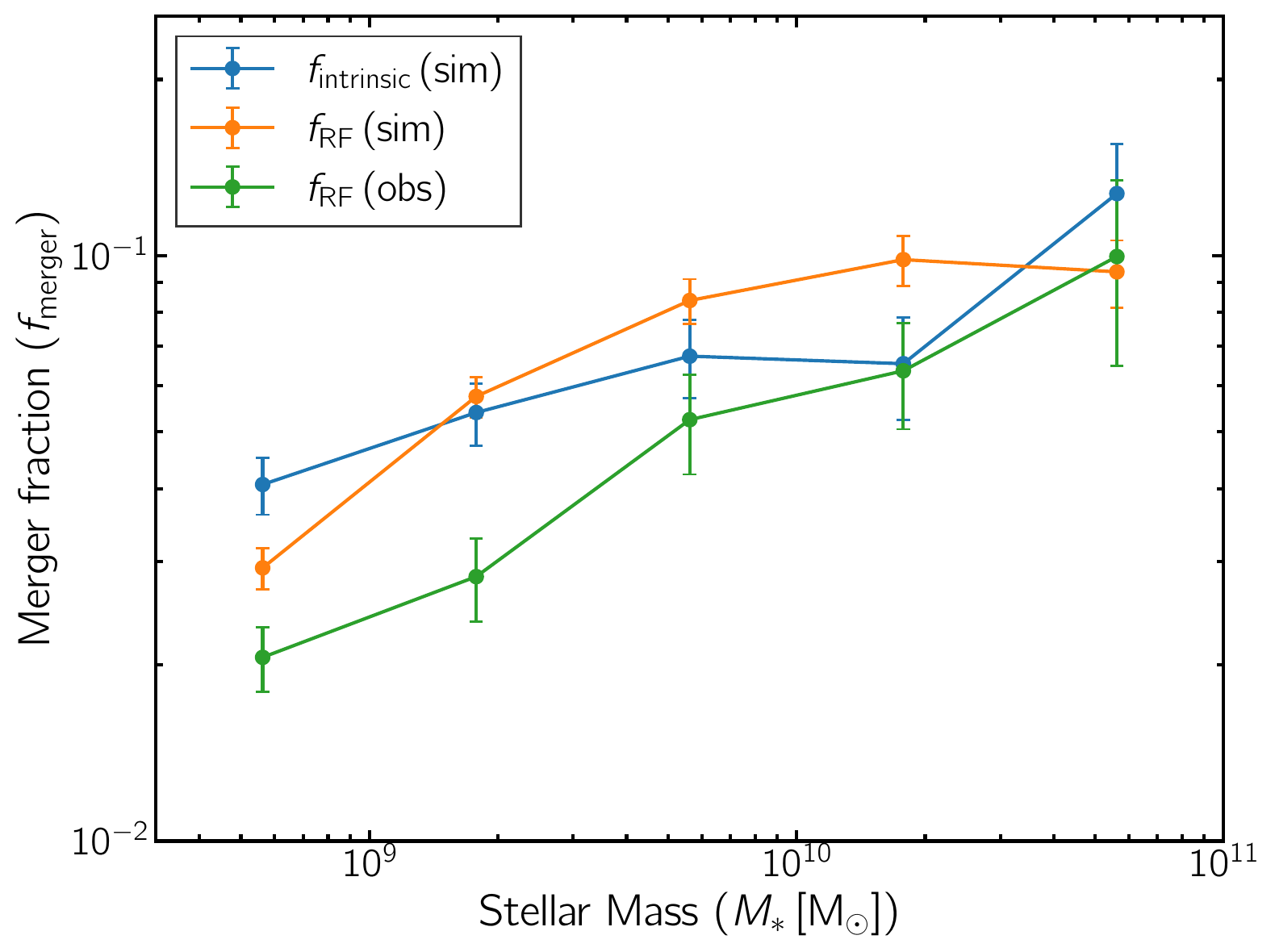
Fig. 12a shows the estimated merger fraction, as a function of stellar mass, for the simulated and observational samples. As can be seen, both follow a qualitatively similar trend to the intrinsic merger fraction, but show differences within a factor of ${\sim}2$, as discussed below. The error bars in the estimated merger fractions are given by Poisson statistics from the number of mergers in each bin. The fact that the random forest classifier predicts a lower merger fraction for observed galaxies than for simulated ones is perhaps not surprising by noting that the most important feature for the classifications is the asymmetry parameter (Section 3.3), and that observed galaxies have somewhat lower asymmetry values than simulated ones (Section 3.1). A more robust result is that the galaxy merger fraction is an increasing function of stellar mass for all the cases considered.

These findings are in contrast with the major merger fraction estimate by Casteels et al. (2014), who found a decreasing merger fraction within the stellar mass range $9.0\leq\log\quantity(M_{\ast}/\mathrm{M}_{\odot})\leq 9.5$, and a roughly constant trend above that mass range, while all of our estimates indicate that the merger fraction increases steadily as a function of stellar mass. This qualitative difference is puzzling, considering that the estimate by Casteels et al., 2014 was performed on a similar observational galaxy sample, using the asymmetry parameter to estimate the fraction of asymmetric galaxies and subsequently the major merger fraction as a function of stellar mass.

For comparison, we have applied an asymmetry-based criterion to our samples to identify highly asymmetric galaxies. These objects were selected as those for which $A>0.25$. In the following step we computed the PPV and TPR for these predictions, and we applied a modified version of eq. 4 to estimate the merger fraction derived from the asymmetry criterion. We note that $\text{PPV}\approx 8.5\%$ and $\text{TPR}\approx 7.5\%$ for this classification, which represents a purity of the same order as that of our RF models but with a completeness that is considerably smaller.

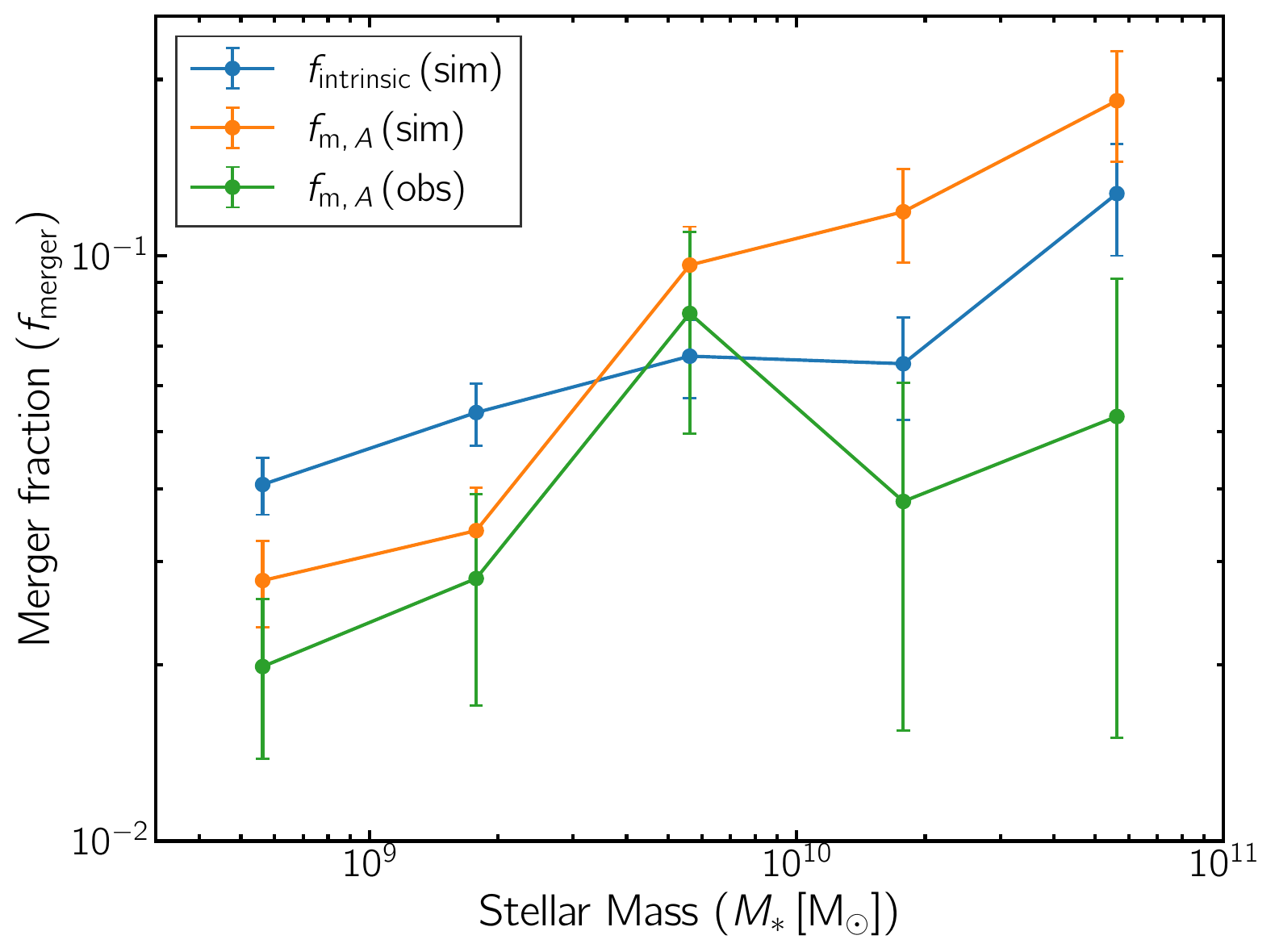
Fig. 12b shows a comparison between the intrinsic merger fraction from the simulation and the asymmetry-based merger fraction, $f_{\mathrm{m},\,A}$, for both simulation and observations. As can be seen, such estimates qualitatively follow the trend of the intrinsic merger fraction: both are increasing functions of stellar mass. However, $f_{\mathrm{m},\,A}(\mathrm{obs})$ is smaller than the other two fractions by a factor of ${\sim}2$, which again reflects the fact that the asymmetry parameter tends to be lower for our observational sample than for our simulated one.

4 Discussion

Using the state-of-the-art TNG50 cosmological simulation and KiDS observations, we have studied the optical morphologies of galaxies at low redshift ($z<0.05$) over a wide range of stellar masses ($8.5<\log_{10}(M_{\ast}/\mathrm{M}_{\odot})<11$). The goal of this analysis has been threefold: (i) to carry out an ‘apples-to-apples’ comparison between the optical morphologies of TNG50 and KiDS galaxies, allowing us to identify possible weaknesses in the IllustrisTNG galaxy formation model at unprecedentedly high mass resolution (16 times better than TNG100); (ii) combining morphological measurements of the simulated galaxies with information from the merger trees, to train and evaluate the performance of an algorithm for identifying merging galaxies based on morphological diagnostics alone; and (iii) to apply this simulation-trained algorithm to observations in order to estimate the galaxy merger fraction in the real Universe.

The first step for carrying out this work was to prepare the observational data set, shown in Figures 1 and 2, which consisted in selecting galaxies from the GAMA catalogues satisfying $8.5\leqslant\log_{10}(M_{\ast}/\mathrm{M}_{\odot})\leqslant 11$ and $z<0.05$, and extracting their corresponding ‘cutouts’ from KiDS mosaic images. Similarly, we prepared a simulation data set by selecting TNG50 galaxies from snapshot 96 (corresponding to $z=0.034$, close to the median redshift of the observational sample) also satisfying $8.5\leqslant\log_{10}(M_{\ast}/\mathrm{M}_{\odot})\leqslant 11$, and then generating synthetic images for all simulated galaxies (including the effects of dust attenuation and scattering, and for three different projections) designed to match the KiDS data set. Fig. 3 shows idealized, composite ($g,r,i$ bands) images for some of our simulated galaxies, while Fig. 4 shows the corresponding $r$-band images after including realism (convolution with a PSF and noise modelling), along with some example galaxies from the observational sample.

After preparing the observational and simulated data sets, we performed source segmentation and deblending on each image in order to isolate the galaxy of interest and remove unwanted or contaminating sources, as illustrated in Fig. 5. We then measured various morphological diagnostics in the $r$-band for galaxies from both data sets using the same code (statmorph), which represents a robust, quantitative comparison between theory and observations. This comparison showed good overall agreement between TNG50 and KiDS galaxies, with the median trend as a function of stellar mass for TNG50 galaxies lying within $\sim$1$\sigma$ of the observational distribution for every morphological parameter considered (Figures 6 and 7). However, TNG50 galaxies tend to be slightly more concentrated and asymmetric than their observational counterparts, and show wider distributions for most parameters.

Interestingly, using the TNG100 simulation, Rodriguez-Gomez et al. (2019) also found that some IllustrisTNG galaxies are more concentrated compared to their observational counterparts from the Pan-STARRS $3\pi$ Survey (Chambers et al., 2016). However, this discrepancy was observed at higher masses, $M_{\ast}\sim 10^{11}\,{\rm M}_{\odot}$, and was attributed to the implementation details of the active galactic nuclei (AGN) feedback – specifically, it was argued that the spherical region over which energy and momentum are injected by the AGN might be too large, and therefore ineffective at small radii. In the present work we reach much lower masses than those achievable in TNG100 (by a factor of 16) and find that the discrepancy pointed out by Rodriguez-Gomez et al. (2019) reappears at $M_{\ast}\sim 10^{9}\,{\rm M}_{\odot}$. Despite the different stellar masses, it is possible that the reason for the higher concentrations of TNG50 galaxies at $M_{\ast}\sim 10^{9}\,{\rm M}_{\odot}$ relative to observations is essentially the same as that for TNG100 galaxies at $M_{\ast}\sim 10^{11}\,{\rm M}_{\odot}$, namely, inefficient AGN feedback at the smallest radii. While the AGN feedback implementation operates in very different modes in such different mass ranges (‘thermal’ versus ‘kinetic’; Weinberger et al. 2017), the size of the ‘injection region’ is determined by the same prescription in both feedback modes (a sphere enclosing an approximately fixed number of gas cells). It will be interesting and important to explore in future galaxy formation models whether reducing the size of the injection region for AGN feedback produces galaxies with concentrations in better agreement with observations. We note, however, that TNG50 produces deficits in the star formation density on small scales that agrees well with observations (Nelson et al., 2021)

On the other hand, the slightly higher asymmetries of TNG50 galaxies compared to observations could simply be a matter of resolution. Young stellar populations, in particular, are undersampled in hydrodynamic cosmological simulations, and manifest as bright clumps that become more noticeable in synthetic images produced with ‘bluer’ broadband filters (Torrey et al., 2015). In principle, this issue could be mitigated by resampling the young stellar populations at a higher resolution (Trayford et al., 2017). However, such procedures would introduce additional complexity to our modelling and, importantly for our goal of characterising galaxy morphology, it is unclear what would be an appropriate spatial distribution for the resampled stellar populations. Therefore, we have adopted the simpler approach of smoothing the light contribution from every stellar particle using the same SPH-like kernel, regardless of the age of the stellar population. A related issue is that the outskirts of simulated galaxies are subject to particle noise, which could further contribute to overestimating the asymmetry parameter. It seems plausible that the asymmetries of simulated galaxies will automatically become more realistic with improved resolution, without the need to make substantial changes to the galaxy formation model.

Having compared the optical morphologies of TNG50 galaxies to those from KiDS observations, we proceeded to compare the morphologies of merging and non-merging galaxies in the simulation. In order to do this, we first defined a merger sample composed of simulated galaxies that experienced a major or minor merger (i.e. those with stellar mass ratio $\mu>1/10$) within a time window of approximately $\pm 0.5$ Gyr. We found that the morphology distributions of our merging and non-merging samples show a large degree of overlap, with the exception of the asymmetry-based statistics, as shown in Figures 8 and 9. However, despite such visually similar morphological distributions of our merging and non-meging samples, it is in principle possible that a combination of various morphological parameters would encode information about the merger histories of the galaxies that is unavailable when using the morphological parameters individually.

To this end, we trained RFs using several combinations of morphological parameters of TNG50 galaxies as the model features, along with the merger label (0 or 1 for our non-merging and merging samples, respectively) as the ground truth, finding in all cases that the most important feature for identifying mergers is the asymmetry statistic. Therefore, the performance of our RF algorithm, usually quantified by the so-called ROC curve, is comparable to that of the more traditional method of selecting highly asymmetric galaxies, but is superior to a direct application of the Gini–$M_{20}$ merger statistic (Fig. 10). Fig. 11 shows some examples of the galaxy merger classifications (both successful and unsuccessful) returned by our RF algorithm.

The high importance of the asymmetry parameter might appear to be in tension with Snyder et al. (2019), where the bulge indicators ($F(G,M_{20})$, concentration) had similar or greater importance than the asymmetry statistic, and the RFs clearly outperformed asymmetry alone. We attribute these differences to the distinct nature of the galaxies considered: massive galaxies ($M_{\ast}>10^{10}\,\text{M}_{\odot}$) at high redshifts in the case of Snyder et al. (2019), and dwarf galaxies (mostly $M_{\ast}\lesssim 10^{10}\,\text{M}_{\odot}$) at low redshifts in the present work. In fact, the RF classification models by Rose et al. (2022) indicate that the asymmetry parameter is more significant for identifying mergers at low redshift than indicators of bulge strength (such as the concentration and Gini statistics), while the latter have a higher importance for high-redshift events. These findings help to reconcile our results with those of Snyder et al. (2019). Another possible factor is the choice of broadband filters. The varying importance of different image-based merger diagnostics in different redshift and stellar mass ranges, as well as for different broadband filters, will be explored in upcoming work.

Finally, we applied our RFs to a test sample from the TNG50 simulation and to the observational sample, in order to estimate the galaxy merger fraction as a function of stellar mass in both simulations and observations (Fig. 12a). In the case of the simulation, our RF was able to recover the ‘intrinsic’ merger fraction (obtained directly from the merger trees) reasonably well (within a factor of $\sim$2). When applied to KiDS observations, our RF returned a galaxy merger fraction that increases steadily with stellar mass, just like the intrinsic merger fraction in TNG50, although with a systematic offset of a factor of $\sim$2. For comparison, we repeated this experiment using the asymmetry statistic alone, separating mergers from non-mergers using a ‘standard’ cut at $A=0.25$ (Fig. 12b). This yielded a steadily rising merger fraction in both simulations and observations, but again with a persistent offset between the two data sets, with the observational merger fraction lying a factor of $\sim$2–3 below the simulation trend. This offset probably reflects the fact that our simulated galaxies are slightly more asymmetric than their observational counterparts.

The results shown in Fig. 12 imply that the merger fraction increases steadily with stellar mass, both when using the RF or the asymmetry parameter alone. These findings are qualitatively consistent with those of Besla et al. (2018), who considered a low-redshift dwarf galaxy ($0.013<z<0.0252$; $2\times 10^{8}\,\text{M}_{\odot}<M_{\ast}<5\times 10^{9}\,\text{M}_{\odot}$) sample from SDSS to compute and compare the major pair fraction (the fraction of primary dwarf galaxies that have a secondary with a stellar mass ratio $\mu>1/4$) with estimations from the original Illustris simulation, also finding an increasing trend (their fig. 14). However, our results are in stark contrast with those of Casteels et al. (2014), who found a decreasing merger fraction over a comparable stellar mass range (their fig. 13), also using the asymmetry statistic as a merger indicator.

5 Summary and outlook

We have carried out an ‘apples-to-apples’ comparison between the optical morphologies of galaxies from the high-resolution, state-of-the-art TNG50 simulation and those of a comparable galaxy sample from KiDS observations. Overall, we have found good agreement between the simulated and observed data sets, which is remarkable considering that the IllustrisTNG galaxy formation model was not tuned to match morphological observations. The TNG50 galaxies, however, are somewhat more concentrated and asymmetric than their observational counterparts. Using additional information from the simulation that is not available in observations – namely, the merger trees – we have trained a random forest algorithm to classify merging galaxies using image-based morphological diagnostics, and applied the random forest to observations in order to estimate the merger fraction in the real Universe. We found that the asymmetry statistic is the single most useful parameter for identifying galaxy mergers, at least in the mass and redshift regime we considered ($8.5\leqslant\log(M_{\ast}/\text{M}_{\odot})\leqslant 11$; $z<0.05$), and that the merger fraction is a steadily increasing function of stellar mass for both the simulated and observational samples.

Currently, it is still challenging to precisely determine the merger fraction in observations, especially using galaxy morphology alone. However, we are approaching an era in which galaxy formation models will become so realistic that it will be possible to exploit subtle trends in morphological measurements – such as the ones studied in this paper – to infer properties of galaxies that are not directly observable in the real Universe, such as their merging histories or even the assembly histories of their host DM haloes. At the same time, our work highlights the importance of developing sophisticated tools to carry out robust comparisons between theory and observations, which will become indispensable in the upcoming years as both computational capacity and astronomical instruments continue to evolve.

Data availability

The data from the IllustrisTNG simulations used in this work are publicly available at the website https://www.tng-project.org (Nelson et al., 2019a). The KiDS and GAMA data are available at the websites http://kids.strw.leidenuniv.nl/ and http://www.gama-survey.org/.

References

- Abraham et al. (1996) Abraham R. G., Tanvir N. R., Santiago B. X., Ellis R. S., Glazebrook K., Bergh S. v. d., 1996, MNRAS, 279, L47
- Abraham et al. (2003) Abraham R. G., van den Bergh S., Nair P., 2003, ApJ, 588, 218
- Baes et al. (2011) Baes M., Verstappen J., Looze I. D., Fritz J., Saftly W., Pérez E. V., Stalevski M., Valcke S., 2011, ApJS, 196, 22
- Baldry et al. (2018) Baldry I. K., et al., 2018, MNRAS, 474, 3875
- Barbary (2016) Barbary K., 2016, JOSS, 1, 58
- Bershady et al. (2000) Bershady M. A., Jangren A., Conselice C. J., 2000, AJ, 119, 2645
- Bertin & Arnouts (1996) Bertin E., Arnouts S., 1996, A&ASS, 117, 393
- Besla et al. (2018) Besla G., et al., 2018, MNRAS, 480, 3376
- Bignone et al. (2016) Bignone L. A., Tissera P. B., Sillero E., Pedrosa S. E., Pellizza L. J., Lambas D. G., 2016, MNRAS, 465, 1106
- Bottrell et al. (2019) Bottrell C., et al., 2019, MNRAS, 490, 5390
- Breiman (2001) Breiman L., 2001, Mach. Learn., 45, 5
- Bruzual & Charlot (2003) Bruzual G., Charlot S., 2003, MNRAS, 344, 1000
- Camps & Baes (2015) Camps P., Baes M., 2015, Astron. Comput., 9, 20
- Casteels et al. (2014) Casteels K. R. V., et al., 2014, MNRAS, 445, 1157
- Chambers et al. (2016) Chambers K. C., et al., 2016, The Pan-STARRS1 Surveys, doi:10.48550/ARXIV.1612.05560, https://arxiv.org/abs/1612.05560
- Chawla et al. (2002) Chawla N. V., Bowyer K. W., Hall L. O., Kegelmeyer W. P., 2002, JAIR, 16, 321
- Conselice (2003) Conselice C. J., 2003, ApJS, 147, 1
- Conselice et al. (2000) Conselice C. J., Bershady M. A., Jangren A., 2000, ApJ, 529, 886
- Crain et al. (2015) Crain R. A., et al., 2015, MNRAS, 450, 1937
- Davis et al. (1985) Davis M., Efstathiou G., Frenk C. S., White S. D. M., 1985, ApJ, 292, 371
- Dolag et al. (2009) Dolag K., Borgani S., Murante G., Springel V., 2009, MNRAS, 399, 497
- Donnari et al. (2019) Donnari M., et al., 2019, MNRAS, 485, 4817
- Dubois et al. (2014) Dubois Y., et al., 2014, MNRAS, 444, 1453
- Duncan et al. (2019) Duncan K., et al., 2019, ApJ, 876, 110
- Ellison et al. (2011) Ellison S. L., Patton D. R., Mendel J. T., Scudder J. M., 2011, MNRAS, 418, 2043
- Ellison et al. (2019) Ellison S. L., Viswanathan A., Patton D. R., Bottrell C., McConnachie A. W., Gwyn S., Cuillandre J.-C., 2019, MNRAS, 487, 2491
- Freeman et al. (2013) Freeman P. E., Izbicki R., Lee A. B., Newman J. A., Conselice C. J., Koekemoer A. M., Lotz J. M., Mozena M., 2013, MNRAS, 434, 282
- Genel et al. (2014) Genel S., et al., 2014, MNRAS, 445, 175
- Groves et al. (2008) Groves B., Dopita M. A., Sutherland R. S., Kewley L. J., Fischera J., Leitherer C., Brandl B., van Breugel W., 2008, ApJS, 176, 438
- Guo & White (2008) Guo Q., White S. D. M., 2008, MNRAS, 384, 2
- Hernquist & Katz (1989) Hernquist L., Katz N., 1989, ApJS, 70, 419
- Hopkins et al. (2010) Hopkins P. F., et al., 2010, ApJ, 715, 202
- Huertas-Company et al. (2015) Huertas-Company M., et al., 2015, ApJS, 221, 8
- Huertas-Company et al. (2019) Huertas-Company M., et al., 2019, MNRAS, 489, 1859
- Kartaltepe et al. (2007) Kartaltepe J. S., et al., 2007, ApJS, 172, 320
- Kewley et al. (2006) Kewley L. J., Geller M. J., Barton E. J., 2006, AJ, 131, 2004
- Kuijken et al. (2019) Kuijken K., et al., 2019, A&A, 625, A2
- Lemaître et al. (2017) Lemaître G., Nogueira F., Aridas C. K., 2017, JMLR, 18, 1
- Lin et al. (2004) Lin L., et al., 2004, ApJ, 617, L9
- Liske et al. (2015) Liske J., et al., 2015, MNRAS, 452, 2087
- Lotz et al. (2004) Lotz J. M., Primack J., Madau P., 2004, AJ, 128, 163
- Lotz et al. (2008) Lotz J. M., et al., 2008, ApJ, 672, 177
- Lotz et al. (2011) Lotz J. M., Jonsson P., Cox T. J., Croton D., Primack J. R., Somerville R. S., Stewart K., 2011, ApJ, 742, 103
- Marinacci et al. (2018) Marinacci F., et al., 2018, MNRAS, 480, 5113
- Martin et al. (2021) Martin G., et al., 2021, MNRAS, 500, 4937
- Naiman et al. (2018) Naiman J. P., et al., 2018, MNRAS, 477, 1206
- Nelson et al. (2018) Nelson D., et al., 2018, MNRAS, 475, 624
- Nelson et al. (2019a) Nelson D., et al., 2019a, Comput. Astrophys., 6, 2
- Nelson et al. (2019b) Nelson D., et al., 2019b, MNRAS, 490, 3234
- Nelson et al. (2021) Nelson E. J., et al., 2021, MNRAS, 508, 219
- Nevin et al. (2019) Nevin R., Blecha L., Comerford J., Greene J., 2019, ApJ, 872, 76
- Patton et al. (2013) Patton D. R., Torrey P., Ellison S. L., Mendel J. T., Scudder J. M., 2013, MNRAS Letters, 433, L59
- Pawlik et al. (2016) Pawlik M. M., Wild V., Walcher C. J., Johansson P. H., Villforth C., Rowlands K., Mendez-Abreu J., Hewlett T., 2016, MNRAS, 456, 3032
- Pearson et al. (2019) Pearson W. J., et al., 2019, A&A, 631, A51
- Pedregosa et al. (2011) Pedregosa F., et al., 2011, JMLR, 12, 2825
- Pillepich et al. (2018a) Pillepich A., et al., 2018a, MNRAS, 473, 4077
- Pillepich et al. (2018b) Pillepich A., et al., 2018b, MNRAS, 475, 648
- Pillepich et al. (2019) Pillepich A., et al., 2019, MNRAS, 490, 3196
- Planck Collaboration XIII (2016) Planck Collaboration XIII 2016, A&A, 594, A13
- Price-Whelan et al. (2018) Price-Whelan a. A. M., et al., 2018, AJ, 156, 123
- Propris et al. (2005) Propris R. D., Liske J., Driver S. P., Allen P. D., Cross N. J. G., 2005, AJ, 130, 1516
- Robitaille et al. (2013) Robitaille T. P., et al., 2013, A&A, 558, A33
- Rodriguez-Gomez et al. (2015) Rodriguez-Gomez V., et al., 2015, MNRAS, 449, 49
- Rodriguez-Gomez et al. (2019) Rodriguez-Gomez V., et al., 2019, MNRAS, 483, 4140
- Rose et al. (2022) Rose C., et al., 2022, arXiv e-prints, p. arXiv:2208.11164
- Schaye et al. (2015) Schaye J., et al., 2015, MNRAS, 446, 521
- Scudder et al. (2012) Scudder J. M., Ellison S. L., Torrey P., Patton D. R., Mendel J. T., 2012, MNRAS, 426, 549
- Sijacki et al. (2015) Sijacki D., Vogelsberger M., Genel S., Springel V., Torrey P., Snyder G. F., Nelson D., Hernquist L., 2015, MNRAS, 452, 575
- Snyder et al. (2015a) Snyder G. F., Lotz J., Moody C., Peth M., Freeman P., Ceverino D., Primack J., Dekel A., 2015a, MNRAS, 451, 4290
- Snyder et al. (2015b) Snyder G. F., et al., 2015b, MNRAS, 454, 1886
- Snyder et al. (2019) Snyder G. F., Rodriguez-Gomez V., Lotz J. M., Torrey P., Quirk A. C. N., Hernquist L., Vogelsberger M., Freeman P. E., 2019, MNRAS, 486, 3702
- Springel et al. (2001a) Springel V., Yoshida N., White S. D. M., 2001a, New Astron., 6, 79
- Springel et al. (2001b) Springel V., White S. D. M., Tormen G., Kauffmann G., 2001b, MNRAS, 328, 726
- Springel et al. (2018) Springel V., et al., 2018, MNRAS, 475, 676
- Stewart et al. (2009) Stewart K. R., Bullock J. S., Barton E. J., Wechsler R. H., 2009, ApJ, 702, 1005
- Taylor et al. (2011) Taylor E. N., et al., 2011, MNRAS, 418, 1587
- Thorp et al. (2019) Thorp M. D., Ellison S. L., Simard L., Sánchez S. F., Antonio B., 2019, MNRAS Letters, 482, L55
- Torrey et al. (2015) Torrey P., et al., 2015, MNRAS, 447, 2753
- Torrey et al. (2019) Torrey P., et al., 2019, MNRAS, 484, 5587
- Towns et al. (2014) Towns J., et al., 2014, Comput. Sci. Eng., 16, 62
- Trayford et al. (2017) Trayford J. W., et al., 2017, MNRAS, 470, 771
- Vogelsberger et al. (2014a) Vogelsberger M., et al., 2014a, MNRAS, 444, 1518
- Vogelsberger et al. (2014b) Vogelsberger M., et al., 2014b, Nature, 509, 177
- Wang et al. (2020) Wang L., Pearson W. J., Rodriguez-Gomez V., 2020, A&A, 644, A87
- Weinberger et al. (2017) Weinberger R., et al., 2017, MNRAS, 465, 3291
- Wen et al. (2014) Wen Z. Z., Zheng X. Z., An F. X., 2014, ApJ, 787, 130
- White & Rees (1978) White S. D. M., Rees M. J., 1978, MNRAS, 183, 341
- Whitney et al. (2021) Whitney A., Ferreira L., Conselice C. J., Duncan K., 2021, ApJ, 919, 139
- de Jong et al. (2013) de Jong J. T. A., et al., 2013, The Messenger, 154, 44
- Ćiprijanović et al. (2020) Ćiprijanović A., Snyder G., Nord B., Peek J., 2020, Astron. Comput., 32, 100390