Mapping the Milky Way Disk with Gaia DR3: 3D extended kinematic maps and rotation curve to $\approx 30$ kpc

Abstract

We apply a statistical deconvolution of the parallax errors based on Lucy’s inversion method (LIM) to the Gaia-DR3 sources to measure their three dimensional velocity components in the range of Galactocentric distances $R$ between 8 kpc and 30 kpc with their corresponding errors and root mean square values. We find results that are consistent with those obtained by applying LIM to the Gaia-DR2 sources, and we conclude that the method gives convergent and more accurate results by improving the statistics of the data-set and lowering observational errors. The kinematic maps reconstructed with LIM up to $R\approx 30$ kpc show that the Milky Way is characterized by asymmetrical motions with significant gradients in all velocity components. Furthermore, we determine the Galaxy rotation curve $V_{C}(R)$ up to $\approx 27.5$ kpc with the cylindrical Jeans equation assuming an axisymmetric gravitational potential. We find that $V_{C}(R)$ is significantly declining up to the largest radius investigated. Finally, we also measure $V_{C}(R)$ at different vertical heights, showing that, for $R<15$ kpc, there is a marked dependence on $Z$, whereas at larger $R$ the dependence on $Z$ is negligible.

;

1 Introduction

The Gaia mission (Gaia Collaboration et al., 2016) is providing the most detailed Milky Way survey to date by measuring stellar astrometry, photometry, and spectroscopy. From this data-set it is possible to derive the spatial distribution, kinematics, and many other physical properties of the Milky Way. The third Gaia data release (DR3) (Gaia Collaboration et al., 2022a) contains the same photometric magnitude and astrometric information of the previous Gaia data EDR3 releases but for a wider sample of stars with new determinations of spectra, radial velocity, chemical abundance, value-added catalogs, etc.

Concerning the kinematics of our Galaxy the Gaia data-sets provide the full astrometric solution - positions on the sky, parallax, and proper motion. Gaia DR3 has also provided a significant increase of the stars line-of-sight velocity catalog, from 7,209,831 in DR2 to 33,812,183 in DR3 (Katz et al., 2022).

Since the first data release, Gaia has played a major part in revealing the kinematics of our Galaxy. Antoja et al. (2016, 2017) used Gaia DR1 and mock data to probe the influence of the spiral arms on Galactic kinematics, found that the typical difference in transverse velocity at symmetric longitudes is about 2 km s^-1, but can be larger than 10 km s^-1 at some longitudes and distances.

By using the DR2, Gaia Collaboration et al. (2018) revealed streaming motions in all three velocity components and found that the vertical velocities show a superposition of modes. The same work found small amplitude perturbations in the velocity dispersion as well.

Kawata et al. (2018) have carried out a kinematic analysis for a radii $R<13$ kpc, a range in which the relative error in the distance was lower than 20 %. Poggio et al. (2018) extended the analyzed region up to $R<15$ kpc in combination with 2MASS photometry, with the aim of characterizing vertical motions. By using around 5 million stars from the Gaia DR2 catalog belonging to the Milky Way disk, Ramos et al. (2018) have also detected many kinematic asymmetries whose azimuthal velocity decreased with the galactic radius.

López-Corredoira & Sylos Labini (2019) have presented extended kinematic maps of the Galaxy with Gaia DR2 including the region where the relative error in distance was between 20$-$100%. That was possible thanks to the use of a statistical deconvolution algorithm of the parallax errors named Lucy’s inversion method (LIM) ( Lucy (1974) and reference therein).

By applying this method to the Gaia-DR2 data-set, and including line-of-sight velocity measurements, López-Corredoira & Sylos Labini (2019) have extended the range of distances for the kinematic analyses of $\approx 7$ kpc with respect to those presented by Gaia Collaboration et al. (2018), thus adding the range of Galactocentric distances between 13 kpc and 20 kpc to the previous maps. They found velocity gradients of about 40 km s^-1 in the radial and azimuthal directions, 10 km s^-1 in the vertical direction, as well as north-south asymmetries.

Bennett & Bovy (2019) made detailed measurements of the wave-like north-south asymmetry in the vertical stellar counts, which showed some deficits at heights $\approx$ 0.4, $\approx$ 0.9 and $\approx$ 1.5 kpc, and peaks at $\approx$ 0.2, $\approx$ 0.7 and $\approx$ 1.1 kpc. The mean vertical velocity is also found to show a north-south symmetric dip at $\approx$ 0.5 kpc with an amplitude of $\approx$ 2 km s^-1. By using OB stellar samples and RGB samples, Romero-Gómez et al. (2019) found that the median vertical proper motion values show a clear vertical modulation towards the anti-centre.

Antoja et al. (2021) used Gaia EDR3 to reveal that oscillations in median rotational and vertical velocities vary with radius, disk stars having large angular momentum moving vertically upwards and disk stars having slightly lower angular momentum moving preferentially downwards.

Drimmel et al. (2022) traced the spiral structure and kinematics using the young stellar population from the Gaia DR3 data-set and found that the local arms are at least 8 kpc long, the outer arms are consistent with those seen in the HI survey. In addition, by analyzing the RGB samples with measured velocities, they found the streaming motions in the outer disk that may be associated to the spiral arms or bar dynamics.

Our aim in this paper is to derive kinematic maps of the Galaxy up to $R\approx 30$ kpc by applying LIM on the Gaia-DR3 data-set only from the observational points of view. There are two advantages passing from DR2 to DR3: on the one hand the sub-sample including radial velocities extracted from Gaia-DR3 has a fainter magnitude limit, i.e., $G_{RVS}$ = 14 (Katz et al., 2022), than that from Gaia-DR2 ($G_{RVS}$ = 12) and thus many more sources; on the other hand parallax errors become lower passing from DR2 to DR3. Indeed, according to Lindegren et al. (2021) uncertainties are smaller in DR3 with respect to DR2 by a factor 0.80 for parallaxes and positions and by a factor 0.51 for proper motions.

Moreover, by assuming that the Galaxy is in a steady state and that the gravitational potential is axisymmetric, i.e., by neglecting perturbations, we then can determine, by means of the Jeans equation, the velocity rotation curve $V_{C}(R)$ or $V_{\phi}$ up to $\approx 30$ kpc. This allows us to confirm the recent results by Eilers et al. (2019) who found that the $V_{C}(R)$ is linearly declining up to 25 kpc with a slope of $\approx-1.7\pm 0.1$ $\mbox{km s}^{-1}\mbox{kpc}^{-1}$ (systematic uncertainty of 0.46 $\mbox{km s}^{-1}\mbox{kpc}^{-1}$). In addition, we present estimations of the rotation curve at different heights and we compare them with the results by Chrobáková et al. (2020): most notably, we find, at small radii, a marked dependence of $V_{C}(R)$ on $Z$ which will be shown below.

The paper is structured as follows: in Sect. 2, we briefly describe the Gaia DR3 sample we use in this work. Then in Sect. 3 we outline essential elements of the LIM, while in Sect. 4 we present results about the 3D kinematics and the rotation curve. Finally in Sect. 5 we draw our main conclusions.

2 Gaia-DR3 data

Gaia DR3 Gaia Collaboration et al. (2022a) provides line-of-sight velocities of more than 33 millions sources with a limiting magnitude of $G\approx$ 14. The full astrometric solution has been done as 5-parameter fit for 585 million sources and 6-parameter fit for 882 million sources. While the median parallax uncertainty is 0.01$-$0.02 mas for $G$ <15, 0.05 mas at $G=$ 17, 0.4 mas at $G=$ 20 and 1.0 mas at $G=21$. The uncertainty in the determination of the proper motion is 0.02$-$0.03 mas yr^-1 for stars with $G$ <15, 0.07 mas yr^-1 for stars with $G=17$, 0.5 mas yr^-1 for stars with $G=20$, 1.4 mas yr^-1 for stars with $G=21$ (Lindegren et al., 2021).

Gaia DR3 also contains a release of magnitudes estimated from the integration of Radial Velocity Spectrometer (RVS) spectra for a sample of about 32.2 million stars brighter than $G_{RVS}\approx 14$ (or $G\approx 15$). Sartoretti et al. (2022) has described the data used and the approach adopted to derive and validate the $G_{RVS}$ magnitudes published in DR3. They also provide estimates of the $G_{RVS}$ pass-band and associated $G_{RVS}$ zero-point. Recio-Blanco et al. (2022) has summarized the stellar parametrization of the Gaia RVS spectra (around 5 millions) performed by the GSP-Spec module and published it as part of Gaia DR3. The formal median precision of radial velocities is 1.3 km s^-1 at $G_{RVS}=12$ and 6.4 km s^-1 at $G_{RVS}=14$. The velocities zero-point exhibit a small systematic trend with magnitude starting around $G_{RVS}=11$ and reaching about 400 m s^-1 at $G_{RVS}=14$: to take into account this trend a correction formula is provided. Note the Gaia DR3 velocity scale is in satisfactory agreement with APOGEE, GALAH, GES and RAVE (Katz et al., 2022).

The Gaia-DR3 data-set provides for each star the parallax $\pi$, the Galactic coordinates $(\ell,b)$, the line-of-sight velocity $V_{r}$ and the two proper motions in equatorial coordinates $\mu_{\alpha}\cos\delta$ and $\mu_{\delta}$. These six variables allow to place each star in the 6D phase space, i.e., 3D spatial coordinates plus 3D velocity coordinates. The Galactocentric position in cylindrical coordinates has components: $R$, the Galactocentric distance, $\phi$, the Galactocentric azimuth and $Z$, the vertical distance. The Galactocentric velocity in cylindrical coordinates has components: $V_{R}$, the radial velocity, $V_{\phi}$, the azimuthal velocity, and $V_{Z}$, the vertical velocity. Details to transform respectively $(\pi,\ell,b)$ in Galactocentric cartesian $(X,Y,Z)$ or cylindrical $(R,\phi,z)$ coordinates and $(V_{r},\mu_{\alpha}\cos\delta,\mu_{\delta})$ in $(V_{R},V_{\phi},V_{Z})$ are given in López-Corredoira & Sylos Labini (2019). The 3D velocity we used is obtained by assuming the location of the Sun is R_⊙ = 8.34 kpc (Reid et al., 2014) and Z_⊙ = 27 pc (Chen et al., 2001). We use the solar motion values [U_⊙, V_⊙, W_⊙] = [11.1,12.24,7.25] km s^-1 (Reid et al., 2014). The value of the circular speed of the LSR is 238 km s^-1 (Schönrich et al., 2010). Note that different solar values have negligible effect for this work.

3 Lucy Inversion Method (LIM)

It is known that Gaia parallax uncertainties increase with distance, in particular beyond 5 kpc from the Sun, and that they are also dependent on the star’s magnitude. The large dispersion of parallaxes correspond to a large dispersion of stellar distances: such dispersion affects the value of mean distance at large heliocentric distances, which is indeed overestimated in a direct measurement with respect to the real one. In order to solve the problem of the deconvolution of the Gaussian errors with large root mean square (rms) values and the asymmetric parallax uncertainties, we adopt the LIM. We refer for more details to López-Corredoira & Sylos Labini (2019) where Monte Carlo simulations to test such technique are also presented.

The basic idea of the method is simple: in order to explore Galactic regions where relative parallax error are larger than $20\%$, i.e., for $R>$ 18 kpc, we can reduce the error in the distance determination by making averages over many stars. We thus divide the observed Galactic region into $N_{cells}$ each containing many stars. We want to determine the average value of the velocity components and their dispersion in each cell. The LIM provides the deconvolved distribution of sources along the line-of-sight; for this quantity we can estimate the mean heliocentric distance of all the stars included in a bin centered at parallax $\pi$ and the corresponding variance $\sigma_{\overline{r}}^{2}(\pi)$. It is worth noticing that the LIM is model independent: we can recover information on the stellar distribution without introducing any prior. In addition the LIM does not provide the distance for each star, rather we only have statistical determination of the distance of a three-dimensional cell that typically contains many stars, i.e., in each of the $N_{cell}$ in which we have divided the observed Galactic region. In this way, in each cell we have the estimation of the average values of the distance, velocity components and their corresponding errors.

4 Results

4.1 Velocity asymmetries with DR3

Figure 1: For each velocity component (from top to bottom, respectively, $V_{R}\,,V_{\phi}\,,V_{Z}$) we plot the map reconstructed by the LIM and projected onto the Galactic $(X,Y)$ plane of the average velocity component in km/s (left panels), errors in km/s (middle panels) and rms value in km/s corrected for measurement errors (right panels).

Figure 2: As Fig.1 but including the correction due to the zero-point bias. Note that the zero-point correction particularly affects large radii by introducing a larger noise/signal ratio: for this reason such correction reduces the range of radii where we can reconstruct kinematic properties.

Figure 3: Zoomed version of the radial (upper panel) and vertical (bottom panel) velocity maps shown in Fig.1.

Figure 4: As Fig.1 but the projection is now on the $(X,Z)$ plane with the constraints: $160^{\circ}<\ell<200^{\circ}$, $\frac{\pi}{\Delta\pi}>1$.

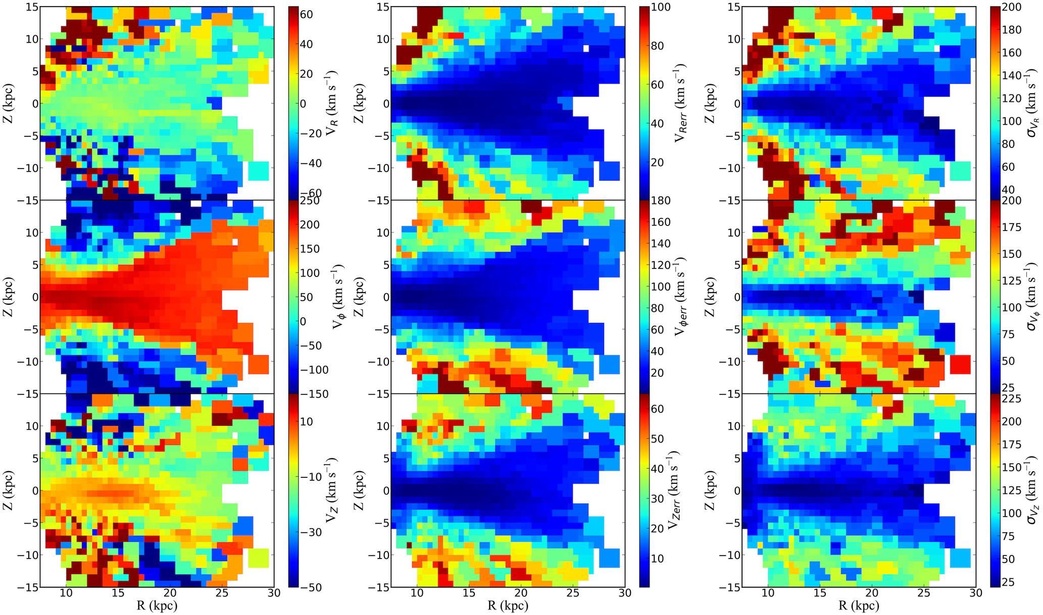
Figure 5: As Fig. 4, but the projection is on the $(R,Z)$ plane.

The LIM gives estimations of the three velocity components, their errors and rms values in the $N_{cells}$ cells in which we have divided the galactic region. Fig.1 shows the maps representing the projection onto the Cartesian $(X,Y)$ plane of the three velocity components $V_{R},V_{\phi}$ and $V_{Z}$ (from top to bottom, left panels), their errors (middle panels) and their rms values (right panels). Note that the deconvolution has included all stars with $\Delta\pi<\pi$ and with $|b|<10^{\circ}$.

The Galactic region within such constraints was divided into 36 line-of-sight, each of them with $\Delta\ell=10^{\circ}$. Then, in each of these cells we have applied the deconvolution technique discussed above. Hereafter only the cells where the number of stars is $N_{stars}\geq 6$ are plotted. The error $\Delta\overline{r}$ in the estimation of the distance $\overline{r}$ is

$$\Delta\overline{r}=\sigma_{\overline{r}}\;.$$ (1)

where $\sigma_{\overline{r}}$ is the dispersion of $\overline{r}$ obtained by the LIM. Note that this is a systematic error and it cannot be reduced by increasing $N_{stars}$ in each cell.

Errors on the velocity components simply are

$$\Delta V_{r}=\frac{\sigma(V_{r})}{\sqrt{N_{stars}}}$$ (2)

$$\Delta\mu_{\ell}=\frac{\sigma(\mu_{\ell})}{\sqrt{N_{stars}}}$$

$$\Delta\mu_{b}=\frac{\sigma(\mu_{b})}{\sqrt{N_{stars}}}\;,$$

i.e., they can be reduced by increasing $N_{stars}$.

As discussed in López-Corredoira & Sylos Labini (2019) we neglect the covariance terms in the errors on $\mu_{\ell}$, $\mu_{b}$ and $\overline{r}$, that is, we assume these errors are independent from each other. Note that rms values plotted in the right panels of Fig.1 were corrected (subtracted quadratically) from the measurement errors of $V_{r}$, $\mu_{\ell}$ and $\mu_{b}$. Uncertainties on $V_{R}$ and $V_{\phi}$ are smaller towards the anti-center because the separation of both components is independent of the distance. Moreover, $V_{R}$ only depends on $V_{r}$, so it is insensitive on the distance errors which instead affect both the determinations of $V_{\phi}$ and $V_{Z}$.

We have tested the impact of the zero-point correction given by Lindegren et al. (2021), using the publicly available Python package, which calculates the zero-point as a function of ecliptic latitude, magnitude, and colour. By comparing Fig.2, that includes the small parallax zero-point bias, with Fig.1 we can conclude that, in line with similar tests presented in López-Corredoira & Sylos Labini (2019), such correction has very minor effects on the derived maps in the region of the anti-center direction, where the detected measurements errors are the smallest ones, while significant differences are found where the errors are larger. However, the region towards the anti-center is the one relevant for the analysis of the velocity profiles that we present below. Indeed, one may note in middle panels of Figs. 1-2 that the error distribution shows a ”horn” like shape, delimiting the region where errors are the smallest ones: the velocity dispersion displays its lower value along $X$ for small (in absolute value) $Y$, i.e., the direction of the anti-center.

The azimuthal velocity map (see 2nd row, left panel of Fig. 1) displays patterns such that $V_{\phi}$ decreases with distance in the range [8,25] kpc, while it increases both for $Y>0$ and $Y<0$. The vertical motions map (see the bottom left panel of Fig.1) presents an “arc shape” similar to the Gaia DR2 map shown in López-Corredoira & Sylos Labini (2019): this is now much better resolved, a fact supporting the robustness of the LIM. Similarly, both the behavior of the error and of the dispersion (middle and right panels of Fig. 1) show the same patterns as in the maps obtained from the analysis of DR2. Fig.3 shows a zoomed version of the the radial and vertical velocity maps presented in Fig. 1.

As seen in Fig. 4, it shows the edge-on projection, i.e., onto the $X,Z$ plane, of the three velocity components (as in Fig.1), with the constraint $160^{\circ}<\ell<200^{\circ}$: this corresponds to the galactic anti-center region. One may note that there are several asymmetries with positive and negative velocity gradients of amplitude from 10 to 25 kpc. The errors become larger between $Z=$ 2 kpc to 4 kpc and between $-$4 kpc to $-$2 kpc and $X\leq$ 15 kpc. Note that in Fig. 4 uncertainties are larger toward the Galactic pole because the binning with constant $\Delta b$ reduces the number of sources in that region.

Fig. 5 shows the projection on the $(R,Z)$ plane, where the vertical coordinate has a broader range, i.e. $Z\in[-15,15]$, one may note asymmetrical kinematics patterns such as radial non-null motions, the ”horn-like” shape in azimuthal velocity and non-zero vertical bulk motions.

Fig. 6 shows the radial velocity profile along the azimuth, in different radial bins and in the range 12$-$24 kpc. At least in the range between $-20^{\circ}$ to $20^{\circ}$, the larger is the distance and the smaller is the radial velocity; beyond this range in azimuth errors are too large to make a reliable estimation of the velocity. Figure 7 shows the vertical velocity profile along the azimuth in different radial bins and in the range 4$-$20 kpc. In addition, $V_{Z}(\phi)$ increases from 4 to 16 kpc, i.e. the larger is the distance the larger is the average vertical velocity.

Finally, the velocity maps and profiles (see below) obtained with the Gaia DR3 are consistent with those obtained by López-Corredoira & Sylos Labini (2019) with Gaia DR2, a fact that shows that the LIM is a robust and reliable technique. This same result can be inferred by a simple visual comparison of Fig. 1 with Fig. 8 of López-Corredoira & Sylos Labini (2019) and of Fig. 4 with their Fig. 9: the maps derived from DR3 well agree with those of DR2 even when we consider the region of DR2 where errors are larger.

4.2 Asymmetric motions: a qualitative view

The maps presented in Figs.1-5 show the complexity and richness of the velocity field of the Galactic disc. They again confirm that the Galactic disk is out-of-equilibrium and it is characterized by asymmetric streaming motions with significant gradients in all velocity components. These results are in agreement with several others in the literature: indeed many velocity substructures, moving groups, bulk motions, radial motions, ridges, snails, arches, etc., have been revealed in recent works using star counts and kinematic observations: see, e.g., Widrow et al. (2012); Gaia Collaboration et al. (2018); Antoja et al. (2018); Wang et al. (2018, 2020); Gaia Collaboration et al. (2021); Recio-Blanco et al. (2022); Katz et al. (2022).

We will present in a forthcoming work a detailed analysis of the different dynamical models able to take into account the kinematic properties revealed in this analysis. We refer the reader for a discussion of a number of theoretical possibilities to López-Corredoira et al. (2020): these include a decomposition of bending and breathing modes, the long bar or bulge, the spiral arms, a tidal interaction with Sagittarius dwarf galaxy, and the analysis of out-of-equilibrium effects.

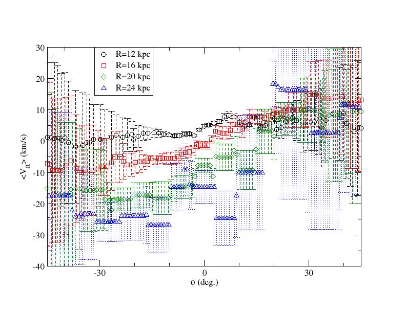
Figure 6: Radial Galactocentric velocity median value as a function of $\phi(\overline{r})$ for different $X(\overline{r})$ (in bins of size $\Delta X=0.5$ kpc) within $|b|<10^{\circ}$.

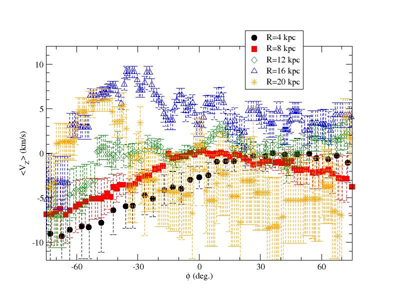
Figure 7: Vertical Galactocentric velocity median value as a function of $\phi(\overline{r})$ for different Galactocentric radii (in bins of size $\Delta R=0.5$ kpc) within $|b|<10^{\circ}$.

4.3 Rotation curve and radial velocity profiles

We now discuss the determination of the radial profiles of the three velocity components at different vertical heights. We then consider the derivation of the velocity rotation curve from the Jeans equation, stressing the underlying hypotheses, and then we describe in detail our results comparing them, in particular, with those of Eilers et al. (2019).

4.3.1 Estimation of velocity moments

As mentioned above, the LIM gives estimations of the velocity components and their dispersion, i.e., $(V_{\alpha}^{i},\;\sigma_{V_{\alpha}}^{i})$ with $\alpha=R,\phi,Z$ in the $i=1,..,N_{cells}$ cells in which we have divided the galactic region. Thus we can estimate the average velocity components as

$$\overline{V_{\alpha}}=\frac{\sum_{i}\frac{V_{\alpha}^{i}}{(\sigma_{V_{\alpha}}^{i})^{2}}}{\sum_{i}\frac{1}{(\sigma_{V_{\alpha}}^{i})^{2}}}\;.$$ (3)

Note we compute in bins of size $\Delta R=1$ kpc and at different heights in $Z_{min},Z_{max}$: for each $R$ the sums in Eq.3 include all the cells such that satisfy such constraints. The estimation of variance the of $\overline{V_{X}}$ is

$$\sigma_{\overline{V_{\alpha}}}^{2}=\frac{1}{\sum_{i}\frac{1}{(\sigma_{V_{\alpha}}^{i})^{2}}}$$ (4)

with the same constraints as before.

4.3.2 Results for velocity profile

Fig. 8 shows respectively the transversal, radial and vertical velocity profiles along the radial distance and computed in different vertical slices of size $\Delta Z$ (left panels) and in bins of size $\Delta Z=1$ centered at $Z_{c}$ plus bins of size $\Delta Z=1$ centered at $-Z_{c}$ (right panels). Hereafter we will refer to these two determinations as integral and differential velocity profiles.

The average azimuthal velocity profile (Fig. 8 top left panel) shows a clear monotonic decreasing trend from $\sim 220$ km ^-1 at $R\approx 10$ kpc to $\sim 160$ km ^-1 at $R\approx 30$ kpc. The differential determination of the azimuthal velocity displays a significant trend at small radii, i.e. for $R<15$ kpc $V_{\phi}$ decreases as $|Z_{c}|$ increases (top right panel of Fig. 8). Instead for $R>15$ kpc, $V_{\phi}$ does not show significant variations with $Z$. It should be noticed that for $|Z|>2$ errors in the determination of the azimuthal velocity are large (up to $\approx 100$ km^-1 — see rms values in the right panel of Fig. 5) and thus these results might require to be confirmed by further data release where the error on the parallax will be lowered.

The radial velocity profile on the Galactic plane (i.e., $Z_{c}=0$) (Fig. 8 middle panels) decreases in function of radius for $R<20$ kpc. Instead, the larger is $Z_{c}$ and the larger the positive value of $V_{R}$, that reaches $\approx 30$ km ^-1 in the outermost regions explored.

Finally, the average vertical velocity (Fig. 8 bottom panels) shows a decreasing trend on the Galactic plane (i.e., $Z_{c}=0$) for $R>$ 15 kpc with a gradient of $20$ km ^-1 until 30 kpc.

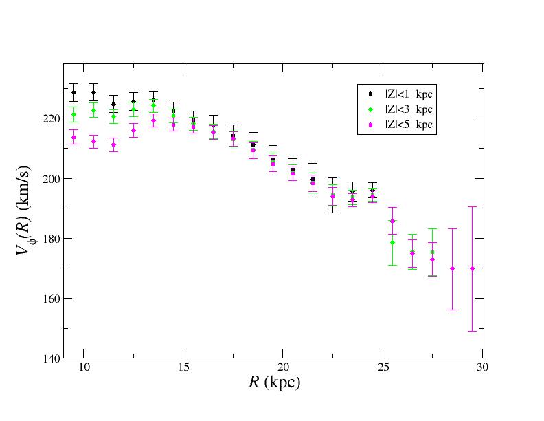
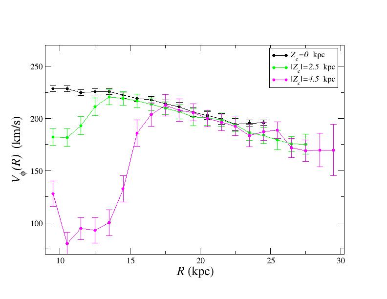
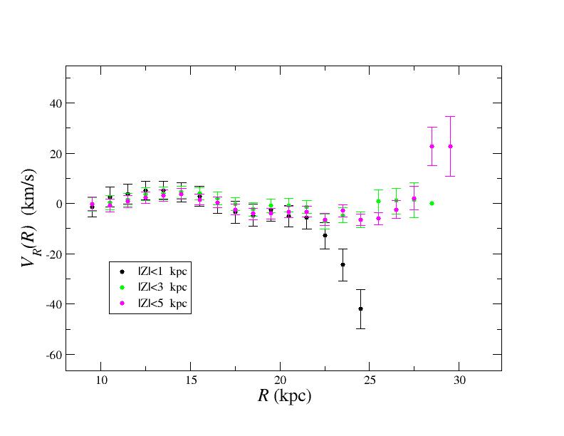
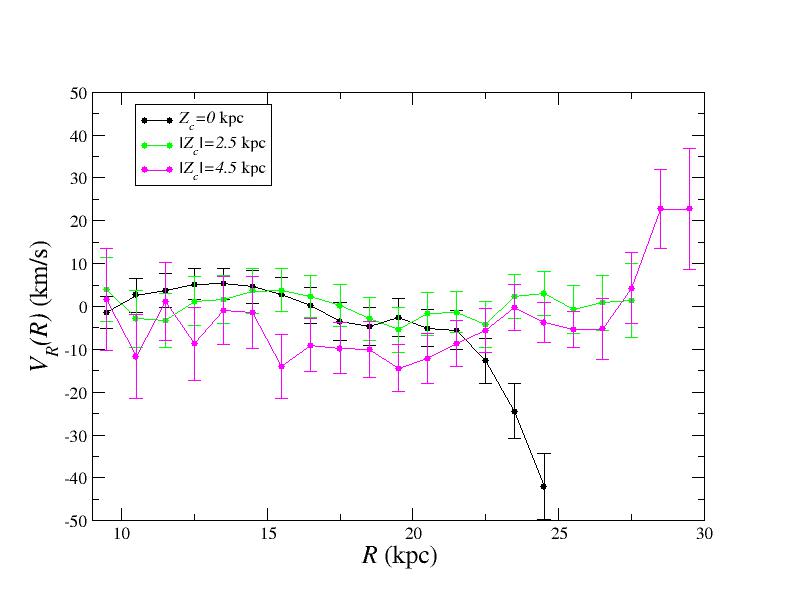
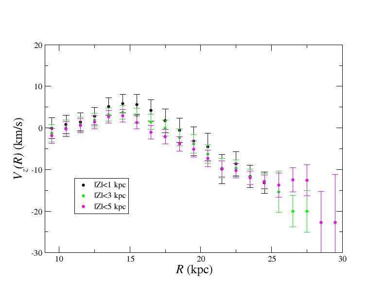
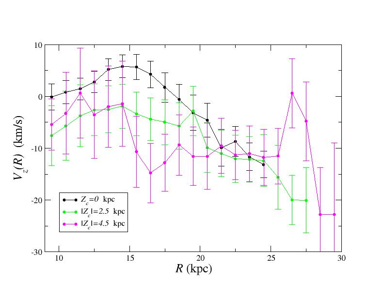
Figure 8: From top to bottom: azimuthal, radial and vertical velocity profile for the DR3 data-set (in the anti-center region with the constraint $160^{\circ}<\ell<200^{\circ}$) in different bins with vertical height in the range $(-Z,Z)$ (left panels) and in vertical bins of size $\Delta Z=2$ half centered in $-Z_{c}$ and half in $Z_{c}$ (right panels).

The effect of the zero-point correction on the velocity profiles is shown in Fig.9. As noticed above the zero-point correction affects the behavior at large radii by introducing larger errors and for this reason such correction reduces the range of radii where we can reconstruct kinematic properties. We find that the velocity profiles, when computed in the same galactic region, nicely overlap.

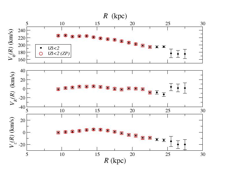
Figure 9: Comparison of the profiles with and without the zero-point correction computed in the same galactic region.

4.3.3 The Jeans Equation

A basic assumption often used to interpret Galactic dynamics is that the disk is in equilibrium or that the gravitational potential is stationary: this hypothesis is definitely challenged by the rich complexity of velocity sub-structures reveled by the 3D kinematic maps provided by the Gaia mission. Theoretically it is not evident how to take into account such streaming motions in all velocity components to construct a self-consistent description of the galaxy. In what follows we will use the time-independent Jeans equation in an axisymmetric gravitational potential to compute the rotation curve. Chrobáková et al. (2020) have shown that, as long the amplitude of the radial velocity component is small compared to that of the azimuthal one, the Jeans equation provides a reasonable approximation to the system. From our analysis we may conclude that up to 30 kpc on the Galactic plane perturbations in the radial velocity should be small and thus we may use the Jeans equation to compare observations with theoretical models.

Assuming an axisymmetric gravitational potential of the Milky Way, we use the the Jeans equation (in cylindrical coordinates $R,Z,\phi$) (Binney & Tremaine, 2008), to link the moments of the velocity distribution and the density of a collective of stars to the gravitational potential, i.e.,

$$\frac{\partial\nu\langle V_{R}\rangle}{\partial t}+\frac{\partial\nu\langle V_{R}^{2}\rangle}{\partial R}+\frac{\partial\nu\langle V_{R}V_{Z}\rangle}{\partial z}+$$ (5)

$$\nu\left(\frac{\langle V_{R}^{2}\rangle-\langle V_{\phi}^{2}\rangle}{R}+\frac{\partial\Phi}{\partial R}\right)=0$$

where $\nu$ denotes the density distribution.

The circular velocity curve in an axisymmetric gravitational potential $\Phi$ of a disk galaxy is defined as

$$V^{2}_{c}(R)=R\frac{\partial\Phi}{\partial R}|_{z\approx 0}\;.$$ (6)

By assuming a steady state, the time dependent term in Eq.5 is set to zero and we get

$$V_{c}^{2}=\langle V_{\phi}^{2}\rangle-\langle V_{R}^{2}\rangle\left(1+\frac{\partial\ln\nu}{\partial\ln R}+\frac{\partial\ln\langle V_{R}^{2}\rangle}{\partial\ln R}\right)+\frac{\partial\nu\langle V_{R}V_{z}\rangle}{\partial z}\;.$$ (7)

We assume that the volume density can be written as

$$\nu(R,z)=\rho_{0}\exp\left(-\frac{R}{h_{R}}\right)\exp\left(-\frac{|z|}{h_{z}}\right)\;,$$ (8)

where $h_{R}$ is the scale length of the disk and $h_{z}$ is the scale height (we use the same values of Chrobáková et al. (2020)). By defining for the three velocity components

$$\langle V_{X}^{2}\rangle=\langle V_{X}\rangle^{2}+\sigma^{2}_{\langle V_{X}\rangle}$$ (9)

we find that Eq.7 can be written as

$$V_{c}^{2}=\langle V_{\phi}\rangle^{2}+\sigma^{2}_{\langle V_{\phi}\rangle}+\left(\langle V_{R}\rangle^{2}+\sigma^{2}_{\langle V_{R}\rangle}\right)\frac{R-h_{R}}{h_{R}}$$ (10)

$$-2R\langle V_{R}\rangle\frac{\partial\langle V_{R}\rangle}{\partial R}-R\frac{\partial\sigma^{2}_{\langle V_{R}\rangle}}{\partial R}+$$

$$\frac{R}{h_{z}}\frac{z}{|z|}\langle V_{R}V_{z}\rangle-R\frac{\partial\langle V_{R}V_{z}\rangle}{\partial z}\;.$$

4.3.4 Rotation curve

Following Eilers et al. (2019) we have neglected the terms with $V_{Z}$ in Eq. 10, because the cross-term $\langle V_{R}V_{Z}\rangle$ and its vertical gradient is $\approx$ 2-3 orders of magnitude smaller compared to the remaining terms hence their effects is negligible.

The resulting integral and differential rotation curve is reported in Fig. 10 the values for $|Z|<$2 kpc are reported in Tab.1). Note that we limited the analysis to the Galactic plane, i.e. $|Z|<3$ kpc, i.e., in the region where the disc is highly dominant over the stellar halo contribution.

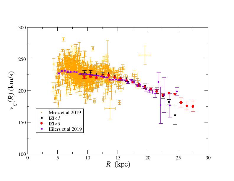
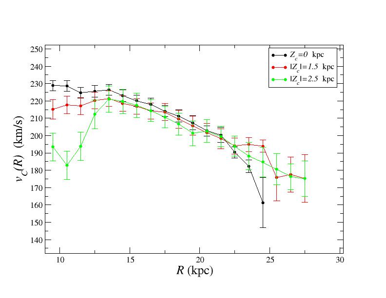
Figure 10: As Fig. 8 but for rotation curve computed in the anti-center region with the constraint $160^{\circ}<\ell<200^{\circ}$; limits on —Z— are reported in the labels. In the left panel data points by Eilers et al. (2019) and by Mróz et al. (2019) are reported for comparison.

$R$ (kpc)	$v_{c}$ (km s-1)	$\sigma_{v_{c}}$ (km s-1)
9.5	221.3	2.5
10.5	222.6	2.4
11.5	220.5	2.4
12.5	222.9	2.4
13.5	224.1	2.2
14.5	220.7	2.3
15.5	218.1	2.3
16.5	215.5	2.4
17.5	213.0	2.6
18.5	209.4	2.9
19.5	205.4	3.1
20.5	201.8	2.7
21.5	198.4	3.3
22.5	194.3	3.5
23.5	193.7	2.4
24.5	194.4	2.1
25.5	178.5	7.4
26.5	175.5	5.8
27.5	175.3	7.7

Table 1: Measurements of the circular velocity of the Milky Way for the Gaia DR3 sample in the anti-center region, i.e. with the constraints $160^{\circ}<\ell<200^{\circ}$ and $|Z|<$3 kpc. Columns show the Galactocentric radius, the circular velocity, and its error bar.

By comparing $V_{C}$ with the azimuthal velocity profile (upper panel of Fig. 8) we notice that the additional terms from the Jeans equation only contributes as small perturbations. In particular, the main features that we have observed for the azimuthal velocity profile are present also for the rotation curve. Namely, the decrease in amplitude passing from 10 kpc to 30 kpc and, when we consider the differential measurement, the trend of the decreasing amplitude at small radii with the increase (in absolute value) of the vertical height. As mentioned above (see Fig.9), we have tested that the systematic contribution due to the zero-point correction does not change significantly the behaviors observed.

That the rotation curve of the Milky Way was decreasing for $R>12$ kpc was also found by several authors with different tracers and modelling (see, e.g., Dias & Lépine (2005); Xue et al. (2008); Bovy et al. (2012); Kafle et al. (2012); Reid et al. (2014); Gibbons et al. (2014); López-Corredoira (2014); Galazutdinov et al. (2015); Gaia Collaboration et al. (2018); López-Corredoira & Sylos Labini (2019); Mróz et al. (2019); Eilers et al. (2019); Jiao et al. (2021); Wang et al. (2022); Bird et al. (2022)). In particular, Eilers et al. (2019) considered a sample with the 6D phase-space coordinates of 23,000 luminous red giant stars, with precise parallaxes determined by combining spectral data from APOGEE DR14 with photometric information from WISE, 2MASS, and Gaia DR2. They measured that the circular velocity curve shows a gentle but significant decline with increasing radius and can be well approximated by a linear function up to 25 kpc:

$$V_{C}(R)=V(R_{\odot})+\beta(R-R_{\odot})$$ (11)

where $R_{\odot}$ is the distance of the Sun from the Galactic center, $V(R_{\odot})=229\pm 0.2\;\mbox{km s}^{-1}$ and the slope was found to be $\beta=-(1.7\pm 0.1)\;\mbox{km s}^{-1}\mbox{kpc}^{-1}$. In Fig. 8 we report the rotation curve determined by Eilers et al. (2019) which nicely agrees with our estimation: in turn their results are in good agreement with previous determinations by Kafle et al. (2012); López-Corredoira (2014); Huang et al. (2016) although these three determinations have larger error bars (see Fig.3 of Eilers et al. (2019)).

The result of Eilers et al. (2019) is in reasonably good agreement with another recent analysis of the Milky Way’s circular velocity curve by Mróz et al. (2019) (also reported in Fig.8 for comparison). This was based on a sample of 773 Classical Cepheids with precise distances based on mid-infrared period–luminosity relations coupled with proper motions and radial velocities from Gaia. They found, in the range of radii between 5 kpc and 20 kpc, a somewhat larger slope of $\beta=-(1.4\pm 0.1)\;\mbox{km s}^{-1}\mbox{kpc}^{-1}$. Note from Fig.8 that, however, the number of Cepheids for $R>15$ kpc drops significantly so that the slope $\beta$ was measured on a very limited range of radii.

By extending the rotation curve to 27.5 kpc we find that $\beta=-(2.3\pm 0.2)\;\mbox{km s}^{-1}\mbox{kpc}^{-1}$, which is smaller than the other two determinations mentioned above. However, in the range of radii where they overlap, i.e. for $R<20$ kpc for the determination by Mróz et al. (2019) and for $R<25$ kpc for the one by Eilers et al. (2019), the three measurements are in reasonably good agreement with each other. In this respect we note that our result is independent from those of Mróz et al. (2019) and Eilers et al. (2019) as we used a different data-set and a different method to determine the rotation curve. Namely, we have constructed a coarse-grained sample and we have applied to it a statistical method to measure the average velocity components and their dispersion, which was tested to provide reliable results, rather than analyzing the velocities of individual stars.

In order to estimate systematic uncertainties on the circular velocity curve arising from our data sample, we split the galactic region into two disjoint smaller portions, one with $0$ kpc $<Z<$ 2 kpc and the other one with -2 kpc $<Z<$ 0 kpc (a similar result is obtained by dividing the sample $b>0^{\circ}$ and $b<0^{\circ}$). We have then computed the rotation curve in the two disjointed regions and we have estimated the systematic uncertainties on the circular velocity by the difference between the resulting fit parameters from the two disjoint data sets. We find that the systematic error on the slope of the rotation curve $\beta$ (see Eq.11) is $\approx 0.4$ km s^-1 kpc^-1 which corresponds to a uncertainty of the order of 20%. An additional contribution to the systematic comes from the fact that, for calculating the circular velocity curve from Eq.7, we neglected the cross terms $\langle V_{z}V_{R}\rangle$. The large noise affecting this terms does not allow a precise determination of its effect, but in agreement with Eilers et al. (2019) we estimate it of the order of a few percent.

4.3.5 Discussion

The two determinations of the Galaxy rotation curve by Mróz et al. (2019); Eilers et al. (2019) and the one presented in this work (that up to 20 kpc coincides with the one by López-Corredoira & Sylos Labini (2019))

are different from others reported in the literature (see, e.g. Bhattacharjee et al. (2014); Sofue (2020)) where the rotation curve of the Milky Way did not present a decrease in the range of distances between 15 kpc and 30 kpc. In such estimations $V_{C}(R)$ was measured when, except in few cases, the full three-dimensional velocity information of the tracers was not available, and it has to be reconstructed from only the measured line-of-sight velocity and positional information of various tracer objects in the Galaxy. On the other hand, results by Mróz et al. (2019), Eilers et al. (2019) and by us in this work share the key fact that they are based on different measurements that have an unprecedented precision and accuracy in the determination of the distances and that allow to have information on the 6D phase-space. The knowledge of the phase-space distribution allows to control for possible systematic effects of different kind as for instance that induced by coherent radial and vertical motions. Given the agreement between these determinations we conclude that our results are reliable and that possible systematic effects in the determination of the rotation curve should be marginal: of course, when the next data release of the Gaia mission will be published it will be possible to further test the rotation curve for $R>20$ kpc. This situation actually shows that the better accuracy of the stars distances together with the great amount of new information provided by the Gaia mission is the key improvement to our knowledge of the Galaxy, its kinematics and dynamics.

Concerning the estimation of mass of the Milky Way we note that Eilers et al. (2019), by considering the standard Navarro Frenk and White halo model, found a virial mass of $M=(7.25\pm 0.25)\times 10^{11}M_{\odot}$ which is significantly lower than what several previous studies suggest. The declining trend of the rotation curve continues when we extend the range of radii form 25 kpc to 27.5 kpc, implies that the best fit with a Navarro, Frenk and White halo model (Navarro et al., 1997) should correspond to an even smaller Milky Way virial mass. A detailed discussion of the dynamical implication of these results will be presented in a forthcoming publication.

Another noticeable feature of the circular velocity that we have detected, namely the trend of the decreasing amplitude for $R<15$ kpc with the increase (in absolute value) of the vertical height has, to our knowledge, not been noticed before. A similar study was presented in Chrobáková et al. (2020) with Gaia DR2, reaching distance up to $R\approx 20$ kpc and heights only up to $|Z|<2$ kpc, where these trends are less noticeable. Moreover, the binning of data in Chrobáková et al. (2020) was more finer, meaning that the derivatives in Eq. (10) are more influenced by fluctuations, making them less reliable. Thus the rotation curves of Chrobáková et al. (2020) are less robust than our current analysis and the trends we see now were not noticed then. As for the case of the determination of $V_{\phi}(R,Z)$ we emphasize that for $|Z|>2$ kpc errors in the determination of the azimuthal velocity are large (up to $\approx 100$ km^-1 — see rms values in the right panel of Fig. 5).

5 Conclusion

We have used the Lucy’s inversion model (LIM) to analyze the Gaia DR3 data-set (Gaia Collaboration et al., 2022a). The LIM can solve the deconvolution of large Gaussian errors that affect the measurements of stellar distance and it was previously applied to the DR2 data-set (López-Corredoira & Sylos Labini, 2019): in this way it was possible to derive the kinematic maps of the Galaxy covering a region where the relative error in distance was larger than 20 % thus extending the range of distances for the kinematic analyses with respect to those presented by Gaia Collaboration et al. (2018). The new analysis discussed in the present work allow us to explore a range of Galactocentric distances up to $\approx$ 30 kpc, while the range of distances covered by studies using only stars with distance errors $<20\%$ also increased, by passing from DR2 to DR3, from 13 kpc (Gaia Collaboration et al., 2018) to 18 kpc (Gaia Collaboration et al., 2022b).

The first noticeable results is that the LIM applied to the DR3 data are compatible with the results of DR2 López-Corredoira & Sylos Labini (2019). This is already an important result showing that the LIM method converges: that is, by lowering the parallax errors and by increasing the number of sources, i.e. the measured stars. The results well confirm those obtained earlier in a data-set with less objects and larger errors. As the method is designed to work when the distribution of error is Gaussian, this means that the observational parallaxes error satisfy such condition.

In addition, as second key result of our work, we find that the new extended maps of the Galactic disk cover the regions of the outer disk that are farther from the Galactic center, whose stars reach $R\approx 30$ kpc (López-Corredoira et al., 2018). These maps show that there are large amplitude and coherent streaming motions in all velocity components. In particular, the radial velocity profile shows an increase toward the outermost region of the Galaxy, but off plane, with a detected value of $V_{R}\approx 30$ km s^-1. The azimuthal velocity also shows a clear decreasing trend in function of the radius. In addition, we have found a marked change of $V_{\phi}(R)$ at small radii, i.e. $R<15$ kpc, when we consider its determination at different heights. In summary, the new extended maps confirm that the Galaxy kinematics is characterized by significant coherent streaming motions in all velocity components as found, at smaller radii, by, e.g., Gaia Collaboration et al. (2018); Antoja et al. (2018); López-Corredoira & Sylos Labini (2019); Khoperskov et al. (2020).

By computing the rotation curve through the Jeans equation, assuming that the Galaxy is in a steady state and that the galactic potential is axisymmetric, we found that $V_{c}(R)$ ($V_{\phi}(R)$) shows a significant decline from $\approx 15$ kpc to 30 kpc of more than 50 km s ^-1. This result is in reasonable agreement with the recent findings by Mróz et al. (2019) up to 20 kpc and by Eilers et al. (2019) up to 25 kpc and extends them to 27.5 kpc but with smaller errors. (Of course, the behavior of the rotation curve in this paper agrees with that found by López-Corredoira & Sylos Labini (2019) by applying the LIM on the Gaia DR2 sources). These three results used different samples that have an unprecedented precision and accuracy in the determination of the distances and that allow to have information on the 6D phase space. Another interesting result that we found is that the rotation curve, as well the azimuthal velocity, presents a marked dependence on the height for $R<15$ kpc whereas, in both cases, at larger $R$ the dependence on $Z$ is negligible. In a forthcoming work we will interpret these behaviors at the light of different galactic models providing an estimation of the Galaxy’s mass.

References

- Antoja et al. (2017) Antoja, T., de Bruijne, J., Figueras, F., et al. 2017, A&A, 602, L13, doi: 10.1051/0004-6361/201731060
- Antoja et al. (2016) Antoja, T., Roca-Fàbrega, S., de Bruijne, J., & Prusti, T. 2016, A&A, 589, A13, doi: 10.1051/0004-6361/201628200
- Antoja et al. (2018) Antoja, T., Helmi, A., Romero-Gómez, M., et al. 2018, Nature, 561, 360, doi: 10.1038/s41586-018-0510-7
- Antoja et al. (2021) Antoja, T., McMillan, P. J., Kordopatis, G., et al. 2021, A&A, 649, A8, doi: 10.1051/0004-6361/202039714
- Bennett & Bovy (2019) Bennett, M., & Bovy, J. 2019, MNRAS, 482, 1417, doi: 10.1093/mnras/sty2813
- Bhattacharjee et al. (2014) Bhattacharjee, P., Chaudhury, S., & Kundu, S. 2014, ApJ, 785, 63, doi: 10.1088/0004-637X/785/1/63
- Binney & Tremaine (2008) Binney, J., & Tremaine, S. 2008, Galactic Dynamics (Princeton University Press)
- Bird et al. (2022) Bird, S. A., Xue, X.-X., Liu, C., et al. 2022, MNRAS, 516, 731, doi: 10.1093/mnras/stac2036
- Bovy et al. (2012) Bovy, J., Allende Prieto, C., Beers, T. C., et al. 2012, Astrophys.J., 759, 131, doi: 10.1088/0004-637X/759/2/131
- Chen et al. (2001) Chen, B., Stoughton, C., Smith, J. A., et al. 2001, Astrophys.J., 553, 184, doi: 10.1086/320647
- Chrobáková et al. (2020) Chrobáková, Ž., López-Corredoira, M., Sylos Labini, F., Wang, H. F., & Nagy, R. 2020, Astron.Astrohys, 642, A95, doi: 10.1051/0004-6361/202038736
- Dias & Lépine (2005) Dias, W. S., & Lépine, J. R. D. 2005, Astrophys.J., 629, 825, doi: 10.1086/431456
- Drimmel et al. (2022) Drimmel, R., Romero-Gomez, M., Chemin, L., et al. 2022, arXiv e-prints, arXiv:2206.06207. https://arxiv.org/abs/2206.06207
- Eilers et al. (2019) Eilers, A.-C., Hogg, D. W., Rix, H.-W., & Ness, M. K. 2019, Astrophys.J., 871, 120, doi: 10.3847/1538-4357/aaf648
- Gaia Collaboration et al. (2016) Gaia Collaboration, Prusti, T., de Bruijne, J. H. J., et al. 2016, Astron.Astrophys., 595, A1, doi: 10.1051/0004-6361/201629272
- Gaia Collaboration et al. (2018) Gaia Collaboration, Katz, D., Antoja, T., et al. 2018, Astron.Astrophys., 616, A11, doi: 10.1051/0004-6361/201832865
- Gaia Collaboration et al. (2021) Gaia Collaboration, Antoja, T., McMillan, P. J., et al. 2021, A&A, 649, A8, doi: 10.1051/0004-6361/202039714
- Gaia Collaboration et al. (2022a) Gaia Collaboration, Vallenari, A., Brown, A. G. A., et al. 2022a, arXiv e-prints, arXiv:2208.00211. https://arxiv.org/abs/2208.00211
- Gaia Collaboration et al. (2022b) Gaia Collaboration, Drimmel, R., Romero-Gomez, M., et al. 2022b, arXiv e-prints, arXiv:2206.06207. https://arxiv.org/abs/2206.06207
- Galazutdinov et al. (2015) Galazutdinov, G., Strobel, A., Musaev, F. A., Bondar, A., & Krełowski, J. 2015, Pub.Astron.Soc.Pacific, 127, 126, doi: 10.1086/680211
- Gibbons et al. (2014) Gibbons, S. L. J., Belokurov, V., & Evans, N. W. 2014, MNRAS, 445, 3788, doi: 10.1093/mnras/stu1986
- Huang et al. (2016) Huang, Y., Liu, X. W., Yuan, H. B., et al. 2016, Mon.Not.R.Astr.Soc., 463, 2623, doi: 10.1093/mnras/stw2096
- Jiao et al. (2021) Jiao, Y., Hammer, F., Wang, J. L., & Yang, Y. B. 2021, A&A, 654, A25, doi: 10.1051/0004-6361/202141058
- Kafle et al. (2012) Kafle, P. R., Sharma, S., Lewis, G. F., & Bland-Hawthorn, J. 2012, Astrophys.J., 761, 98, doi: 10.1088/0004-637X/761/2/98
- Katz et al. (2022) Katz, D., Sartoretti, P., Guerrier, A., et al. 2022, arXiv e-prints, arXiv:2206.05902. https://arxiv.org/abs/2206.05902
- Kawata et al. (2018) Kawata, D., Baba, J., Ciucǎ, I., et al. 2018, Mon.Not.R.Astr.Soc., 479, L108, doi: 10.1093/mnrasl/sly107
- Khoperskov et al. (2020) Khoperskov, S., Gerhard, O., Di Matteo, P., et al. 2020, Astron.Astrophys., 634, L8, doi: 10.1051/0004-6361/201936645
- Lindegren et al. (2021) Lindegren, L., Klioner, S. A., Hernández, J., et al. 2021, Astron.Astrophys., 649, A2, doi: 10.1051/0004-6361/202039709
- López-Corredoira (2014) López-Corredoira, M. 2014, Astron.Astrophys., 563, A128, doi: 10.1051/0004-6361/201423505
- López-Corredoira et al. (2018) López-Corredoira, M., Allende Prieto, C., Garzón, F., et al. 2018, A&A, 612, L8, doi: 10.1051/0004-6361/201832880
- López-Corredoira et al. (2020) López-Corredoira, M., Garzón, F., Wang, H. F., et al. 2020, A&A, 634, A66, doi: 10.1051/0004-6361/201936711