What Makes a Good Explanation?: A Harmonized View of Properties of Explanations

Abstract

Interpretability provides a means for humans to verify aspects of machine learning (ML) models and empower human+ML teaming in situations where the task cannot be fully automated. Different contexts require explanations with different properties. For example, the kind of explanation required to determine if an early cardiac arrest warning system is ready to be integrated into a care setting is very different from the type of explanation required for a loan applicant to help determine the actions they might need to take to make their application successful.

Unfortunately, there is a lack of standardization when it comes to properties of explanations: different papers may use the same term to mean different quantities, and different terms to mean the same quantity. This lack of a standardized terminology and categorization of the properties of ML explanations prevents us from both rigorously comparing interpretable machine learning methods and identifying what properties are needed in what contexts.

In this work, we survey properties defined in interpretable machine learning papers, synthesize them based on what they actually measure, and describe the trade-offs between different formulations of these properties. In doing so, we enable more informed selection of task-appropriate formulations of explanation properties as well as standardization for future work in interpretable machine learning.

1 Introduction

Interest in interpretable machine learning has grown in recent years. Regulatory bodies see interpretable machine learning as a method for auditing algorithms for safety, fairness, and other criteria—especially in high-stakes situations. Industry sees interpretable machine learning not only as a mechanism to provide oversight over their products, but also as a way to uncover insights on trends in their data and other forms of human+ML teaming.

It is well-accepted that different contexts will require different kinds of methods for interpretable machine learning. For example, the kind of explanation required to determine if an early cardiac arrest warning system is ready to be integrated into a care setting is very different from the type of explanation required for a loan applicant to help determine the actions they might need to take to make their application successful. Identifying which interpretability methods are best suited to which tasks remains a grand challenge in interpretable machine learning.

We can quantify how "good" an interpretable machine learning method is by quantifying the properties it preserves. Since these properties must be tied to the task it is designed to explain, they can serve as an abstraction between the method and its context. For example, both an explanation describing features a patient might change to reduce future cardiac risk and an explanation describing features a loan applicant might change to successfully get a loan, should clearly have no false positives—if the person acts on the listed features, the output should change. In both cases, it might also be important for the explanation to be reasonably short as the person may not have the time or inclination to parse through a complex description. In contrast, if one were vetting a risk predictor for a health or justice scenario, one might require a more complete explanation of the entire model—and not mind spending time carefully inspecting it. In other words, desirable properties in explanations are completely dependent on the context and the explanation being used, which is why we can consider them as an abstraction between the two. If one knows what properties are needed for what contexts, then one might be able to check for those properties computationally to identify promising interpretable machine learning methods prior to more expensive user studies with people.

Unfortunately, while many works have defined properties, there is little current consensus around the terminology and formulation of interpretable machine learning properties. We highlight some of the issues due to this. First, different works have used different terms for the same property. For example, one work might call a property robustness while another calls it stability. Second, different works have formalized the notion of these properties differently: the expressions that one work uses to computationally evaluate compactness may be different than another. The current state of having multiple definitions in literature and a lack of consistent formulations makes it difficult to compare methods rigorously. It also becomes challenging to interpret what it truly means when one claims that a certain context needs a certain property or that a certain algorithm preserves it.

This paper reviews and synthesizes existing properties and definitions in the interpretable machine learning literature. We first collect together metrics describing the same properties but termed differently in different works. Next, for each property, we (a) precisely describe the various mathematical formulations that have been proposed, (b) identify the key variations in those formulations, and (c) describe how different formulations of the same property might be appropriate in different contexts. Finally, we use these formulations to make precise how different properties may or may not be in tension with each other.

In doing the above, our framework provides a much-needed systematic synthesis of a key part of the interpretable machine learning ecosystem. Our work serves as a reference for not only what are common properties that we might desire of interpretable machine learning methods, but also what considerations might go into how the abstract property is made precise. Our work can serve as a reference for both what terms are used to describe properties as well as how to formalize them for future research in interpretable machine learning.

2 Related Work

The urgent need for explainable and interpretable machine learning has prompted researchers to focus on reviewing and categorizing existing literature based on explainability methods, properties, and evaluation metrics. However, to the best of our knowledge, there has not been prior work that organizes formulations of explanation properties—which is necessary for future work comparing interpretable machine learning methods and understanding what information is needed in what contexts.

Reviews of Explanation Types:

The categorization of explanations into various classes in the form of a taxonomy to aid practical usage has been offered by Arya et al. (2019). Since this work focuses on real-world usage of explanations, they supplement this overview with a software package implementing the explainability methods under various classes. Carvalho et al. (2019) also classify explanation methods based on various criteria such as explanation type, result, scope, etc. Marcinkevics and Vogt (2020) provide a similar non-exhaustive categorization of various explainable and interpretable methods from a quantitative perspective. Similarly, Murdoch et al. (2019) offer a framework which aids the categorization and selection of explainable and interpretable techniques for practical applications. All of these works focus on the types of explanations. In contrast, we categorize formulations of the properties that describe an explanation’s quality.

Reviews of Explanation Properties and Metrics:

The terms property and evaluation metric are often used synonymously in different works. We prefer the term property to avoid conflation with the ultimate downstream evaluation metric—how well an explanation aids a user in performing their task. The identification of important properties in explanations by reviewing various explanation evaluation metrics in literature has been offered by Zhou et al. (2021). Liao et al. (2022) provide a user survey based taxonomy with a focus on desired properties and usage contexts of explanations. Sovrano et al. (2021) offer a review of evaluation metrics based on their compliance with the law and the properties to be satisfied for such compliance, which differs from our focus on the quantitative objectives fulfilled by each property. Unlike these works, we make each property precise by offering an analytical comparison between proposed definitions in literature and by mapping these definitions to various use cases.

Other Taxonomies:

A thorough taxonomy discussing all contributions in explainable machine learning, intended to serve as overarching references for incoming researchers in the field, has been presented by Barredo Arrieta et al. (2020) and Adadi and Berrada (2018). The former discusses explanations and their properties with a focus on the types of models in use. Guidotti et al. (2018) also provide a mapping of explanation methods to the type of black-box model being used in addition to discussing the types of problems they can address. These reviews are broad, and do not focus on the precise concern of synthesizing different property formulations.

3 Notation and Terminology

In this work, we use $f$ to denote the model to be explained and $E(f)$ to represent the explanation; we define the explanation as the information provided from the model to the user. Throughout the work, we look at predictive models that yield a prediction $\hat{y}=f(\mathbf{x})$ for the input point $\mathbf{x}$ that has $K$ features $x^{(1)}\dots x^{(K)}$. For the model $f$, we denote its prediction as $\hat{y}_{f}$, which may be discrete or continuous depending on whether the task is classification or regression. If the explanation depends also on the input, we will use the notation $E(f,\mathbf{x})$. Certain evaluations of explanations also require a baseline or reference input value, we denote $\mathbf{x}_{0}$ as this reference value. Some also take into account the ground truth value at an input $\mathbf{x}$, and we denote $y$ as the respective ground truth. Explanations in the interpretable machine learning literature tend to fall into three main categories: function-based explanations, feature-attribution-based explanations, example-based explanations.

Function-based Explanations:

We use the term function-based explanations for models or structures that are inherently interpretable and allow one to produce an output or reasoning given an input. Typically, this means that the explanation will produce a prediction $\hat{y}_{E}$ that can be compared to the model prediction $\hat{y}_{f}$. Examples are: a local surrogate explanation that uses an interpretable model (e.g. sparse linear model, decision tree, etc.) to approximate the target model locally around an individual prediction; a decision set that approximates the target model’s behavior globally with nested if-else rules; a self-explaining neural network that has an interpretable linear form but with the coefficients being neural networks and depending on the input; a concept bottleneck model that maps features to interpretable concepts and then uses the concepts to predict the output.

Feature Attribution Explanations:

The next common form of explanation is one that simply provides a list of important features (perhaps ordered or weighted somehow). Specifically, a feature attribution explanation $E$ gives a length-$K$ vector, in which each entry $E(f,\mathbf{x})_{k}$ is the attribution score for each feature $k=1\dots K$ at observation $\mathbf{x}$ for model $f$. Different feature attribution methods use different ranges of values for $E(f,\mathbf{x})_{k}$: some may assign both positive and negative weights; others may only assign non-negative weights. The ranking of features $\text{Rank}_{E}(f,\mathbf{x})$ given the attribution weights $E(f,\mathbf{x})_{k}$ is the ordering of the features from largest to smallest.

Sparse feature attribution methods attempt to identify a subset of relevant features from the full set. We use $\mathcal{S}\subseteq\{1\dots K\}$ to represent the retained subset of features. We use $\mathbf{x}_{\mathcal{S}}$ to denote a version of the input $\mathbf{x}$ for which the values of the features in $\mathcal{S}$ are retained, and the values of the features not in $\mathcal{S}$ are reverted to baseline values $\mathbf{x}_{0}$: $\mathbf{x}_{\mathcal{S}}^{(k)}=\mathbf{x}^{(k)}\,\text{if}\,k\in\mathcal{S}\,\text{else}\,\mathbf{x}_{0}^{(k)}$ for $k=1\dots K$. Similarly, we use $\mathcal{S}^{c}$ to denote the complement of $\mathcal{S}$ and $\mathbf{x}_{\mathcal{S}^{c}}$ to denote the input $\mathbf{x}$ with features in $\mathcal{S}^{c}$ retained and features in $\mathcal{S}$ reset to the reference value $\mathbf{x}_{0}$, i.e. $\mathbf{x}_{S^{c}}^{(k)}=\mathbf{x}_{0}^{(k)}$ if $k\in\mathcal{S}$ else $\mathbf{x}^{(k)}$ for $k\in\mathcal{S}^{c}$.

Unlike function-based explanations, a list of feature attributions does not, in itself, provide a way to predict an output given an input. However, one common approach to making predictions given a feature attribution-based explanation $E(f,\mathbf{x})_{k}$ is to compute the prediction $f(\mathbf{x}_{\mathcal{S}})$.

Example-based Explanations:

Example-based methods select a subset of representative samples from the dataset to explain model behavior or the underlying distribution.

Metrics and Norms:

We use $\ell(\cdot,\cdot)$ to denote all norms and specify the type of norm (e.g. $\ell_{2}$ for the $L$-$2$ norm) and what space it is on, in the text.

We often want to compare the model prediction output $\hat{y}_{f}=f(\mathbf{x})$ to the output implied by the explanation $\hat{y}_{E}$. (For function-based explanations, there is a direct way to compute $\hat{y}_{E}=E(f,\mathbf{x})(\mathbf{x})$ for local explanations and $\hat{y}_{E}=E(f)(\mathbf{x})$ for global explanations; for feature attribution methods, we can use heuristics like those listed above.) We use $\mathcal{L}(\hat{y}_{f},\hat{y}_{E})$ to denote the loss that captures how well the explanation captures the model’s behavior at an input $\mathbf{x}$.

Finally, all equations presented in the relevant literature cited below are converted to this notation for ease of comparison. We also reference the original equations to allow the reader to refer to the source.

4 Framework for Synthesizing Properties of Model Explanations

We synthesize explanation evaluation metrics from existing literature and find that they broadly fall under four distinct categories, each of which corresponds to a desired property for model explanations. We provide a visual categorization of the metrics introduced by various works in literature in Figure 1 and synthesize them in their corresponding sections.

Robustness/Sensitivity:

Robustness or sensitivity measures how much the explanation is prone to change when the input $\mathbf{x}$ is changed infinitesimally or imperceptibly. This is an important property because similar inputs should yield similar explanations, else users might rely on inconsistent explanations for slightly variable inputs and lose trust in the model.

Faithfulness/Fidelity:

Faithfulness or fidelity evaluates the explanation’s capability to capture the true underlying decision-making of the model. This is important because explanations should reveal the true reasoning of the model to the users. Failing to do so can affect downstream decision-making by the user and lead to unfavorable outcomes, especially in high-risk scenarios.

Complexity/Compactness:

Complexity or compactness describes the cognitive effort that users would have to exert to understand the explanation. This is an important property because simple explanations are more understandable and thus more usable. We observe a trade-off between faithfulness and complexity, i.e. a tension between accurately capturing model behavior and maximizing user understandability of the explanation.

Homogeneity:

Homogeneity refers to the ability of the explanation to accurately reveal the model’s underlying decision-making across different subgroups, which is equivalent to faithfulness across subgroups. In specific applications, these subgroups differ by a sensitive demographic attribute, which makes homogeneity relevant to fairness preservation. On the other hand, homogeneity can also be viewed as the explanation’s ability to be robust to input perturbations to subgroup membership. From the standpoint of fairness, if a model makes biased/fair decisions, then an explanation that preserves homogeneity should accurately reveal the unfairness/fairness to the user. This makes homogeneity a combination of faithfulness and robustness across subgroups.

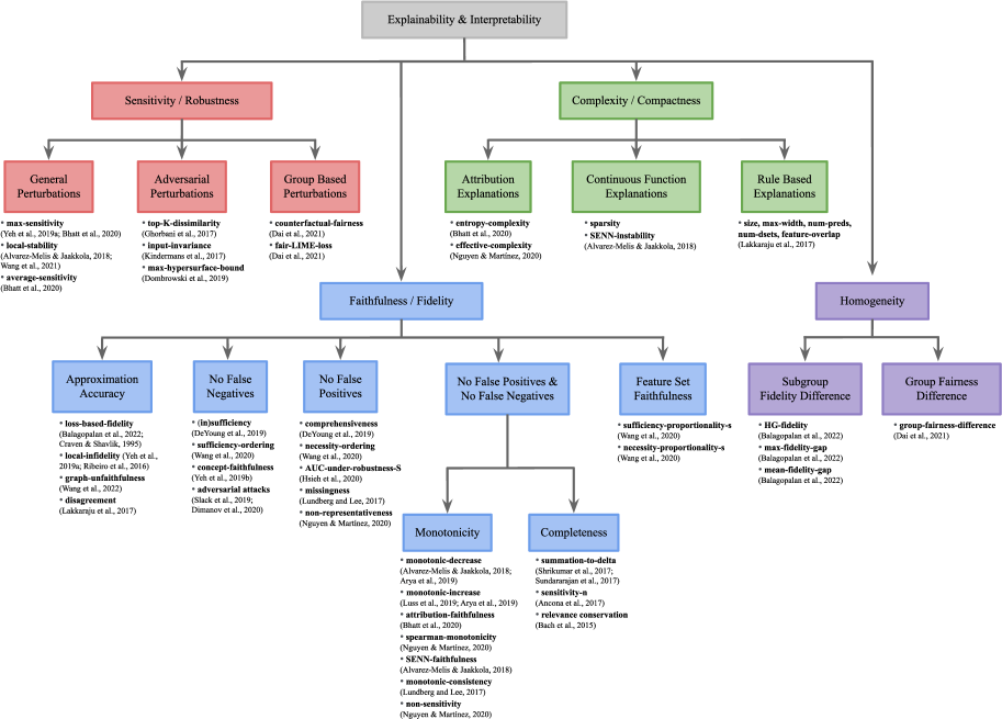
Figure 1: Property Synthesis Framework

What follows is a synthesis of the properties preserved by the various explanation metrics proposed in literature and a categorization by their mathematical formulation, the underlying notion being captured and the human tasks requiring the preservation of these properties.

5 Robustness and Sensitivity

The first property we examine is robustness, also often referred-to as sensitivity. For local interpretability methods (i.e. methods that explain the prediction for a given $\mathbf{x}$), sensitivity measures the similarity of explanations under changes to the input point $\mathbf{x}$. It has been shown that robustness increases user trust in the explanation (Yeh et al., 2019a, Ghorbani et al., 2017): users expect explanations to be stable under minor changes to the input point $\mathbf{x}$. Especially in high-stakes applications, it is important to ensure that minor changes to the input do not lead to explanations that are very different since this could mislead users to inappropriately trust incorrect models. Robust explanations also help manage end-user expectations from the model. Additionally, sensitivity to input perturbations plays a key role in determining the success of an adversarial attack that seeks to perturb the explanation via an imperceptible perturbation of the input.

Input perturbations can be performed in various ways and is typically defined as being performed on a region of interest. For instance, local perturbations are performed within a sphere of a given radius surrounding the input $\mathbf{x}$ and the region here is the sphere itself. Group perturbations are performed by perturbing group membership values of the input $\mathbf{x}$ and the region is characterized by the set of sensitive attribute values. Within a given region, the nature of the perturbation can be general or adversarial and sensitivity is broadly measured as the change in the perturbed and unperturbed explanations, via distance and similarity metrics.

In the following, we categorize and compare proposed mathematical formulations for sensitivity. In all cases, we presume there is some context-dependent definition of similarity between two explanations so that we can numerically calculate the "difference/change in explanation". Then, the formulations for sensitivity fall into three major categories:

• Sensitivity via general perturbations measures the change in explanation as a function of change in input, where this change in input is described via local perturbations of a given radius. It evaluates the collective impact on an explanation when inputs are subject to change and this can be quantified as the maximum change in explanation, the average change in explanation, or the maximum ratio of explanation change to perturbation size. We describe these in Section 5.1.

• Sensitivity via adversarial perturbations is a special case where the perturbations are intended to cause change in explanation while the input is perturbed imperceptibly. These are highly relevant to explanation methods where the input is an image that can be perturbed to deceive the explanation, thus raising security concerns in medical and economic applications. This undesirable explanation change when subject to an adversarial attack is formalized in different ways depending on the region of input perturbation. While most of the current applications have been to images, the general definition can be applied to other use cases. We describe these in Section 5.2.

• Sensitivity via group-based perturbations measures the change in an explanation by changing only the group membership of a sensitive categorical attribute in the input. This type of perturbation can also be viewed as a general perturbation where the geometric region is cylindrical and the perturbation is along a single axis measuring sensitive attribute change. This is relevant to downstream applications which require the explanation to reveal underlying group-based unfairness/biases in the model. In other words, an explanation must be robust enough to accurately reflect the model’s group-based decision making when subjected to group-based perturbations. We describe these in Section 5.3.

We expand on each below.

5.1 Sensitivity via General Perturbations

General perturbations usually refer to random perturbations within a specific region around the original input and the examples in literature use spherical regions for local perturbations and cylindrical regions for group-based perturbations. However, a general definition of sensitivity could use geometric regions of different shapes, depending on the application.

The first metric of sensitivity via general perturbations, proposed by Yeh et al. (2019a) (also discussed by Bhatt et al. (2020)), defines max-sensitivity as the maximum change in the explanation $E$ under a small perturbation. The perturbation is defined within a sphere of radius $r$ around the input $\mathbf{x}$ and the change in explanation is measured by the $\ell_{2}$ norm:

$$\text{max-sensitivity}(E,f,\mathbf{x},r)\triangleq\max_{\left\|\mathbf{x}^{\prime}-\mathbf{x}\right\|\leq r}\left\|E(f,\mathbf{x}^{\prime})-E(f,\mathbf{x})\right\| \triangleright\,\text{Definition 3.1 in \cite[citeauthor]{\@@bibref{Authors}{Yeh2019OnT}{}{}}}$$ (1)

While bounding max-sensitivity bounds the change in explanation within a small region, it does not require continuity. That is, the explanation may change abruptly within the region. In contrast, Alvarez-Melis and Jaakkola (2018) (also discussed in Yeh et al. (2019a)) propose an alternative metric, called local-stability, that measures the ratio of the maximum change in explanation within the perturbation region to the size of the perturbation region (akin to Lipschitz continuity). Again, the change in the explanation $E$ and the distance from $\mathbf{x}$ are both measured by the $\ell_{2}$ norm:

$$\text{local-stability}(E,f,\mathbf{x},r)\triangleq\max_{\left\|\mathbf{x}^{\prime}-\mathbf{x}\right\|\leq r}\frac{\left\|E(f,\mathbf{x})-E(f,\mathbf{x}^{\prime})\right\|}{\left\|\mathbf{x}-\mathbf{x}^{\prime}\right\|} \triangleright\,\text{Equation 5 in \cite[citeauthor]{\@@bibref{Authors}{AlvarezMelis2018}{}{}}}$$ (2)

Wang et al. (2021) refer to robustness for a feature attribution $E$ as a constrained version of Equation 2, wherein an explanation is locally-robust if its $\text{local-stability}(E,f,\mathbf{x},r)\leq\lambda$ for a given threshold $\lambda$.

Unlike max-sensitivity, bounding local-stability ensures that the perturbed input explanations become sufficiently similar to the explanation at input $\mathbf{x}$, as we approach $\mathbf{x}$. In fact, as $r\rightarrow 0$, local-stability converges to the $\ell_{2}$ norm of the gradient of $f$ at $\mathbf{x}$, so it can be easily approximated for small $r$ (assuming that $f$ is differentiable). However, the disadvantage of bounding local-stability is that explanations become insensitive to all small input perturbations, including the ones that cause tangible change to the model prediction.

In cases where the explanation varies smoothly in a region of perturbation except for at a few isolated points, max-sensitivity or local-stability may be unrepresentative of the behavior of the explanation system, as it can be determined completely by these "outlier points". To address this, we can consider average-sensitivity (Bhatt et al., 2020), by looking at the average change in the explanation within the perturbation region. To take the average, they define a distribution $p(\mathbf{x})$, which captures the region of interest. In the simplest formulation, $p(\mathbf{x})$ is uniformly distributed in a sphere with radius $r$ around $\mathbf{x}$: $p=U(\{\mathbf{x}^{\prime}|\left\|\mathbf{x}^{\prime}-\mathbf{x}\right\|\leq r\})$. To measure the change in the explanation we use $\ell_{2}$ distance, although in the original formulation the metric is stated with a general distance metric.

$$\text{average-sensitivity}(E,f,\mathbf{x},p)\triangleq\int_{\mathbf{x}^{\prime}\in\mathrm{R}^{K}}\left\|E(f,\mathbf{x})-E(f,\mathbf{x}^{\prime})\right\|p(\mathbf{x}^{\prime})\ \mathrm{d}\mathbf{x}^{\prime} \triangleright\,\text{Definition 2 in \cite[citeauthor]{\@@bibref{Authors}{Bhatt2020}{}{}}}$$ (3)

An additional benefit of average-sensitivity is that one can obtain an unbiased estimate by drawing Monte-Carlo samples from $p(\mathbf{x})$. The same does not hold for max-sensitivity and local-stability. Further, explanation aggregation can be used as a means for minimizing average-sensitivity.

5.2 Sensitivity via Adversarial Perturbations

While general perturbations usually refer to random perturbations in a geometric region surrounding the original input, adversarial perturbations refer to well-designed perturbations on some targeted features in a specific direction such that the change in model behavior is infinitesimal while the explanation undergoes considerable change, i.e. is highly sensitive. The goal with adversarial perturbations is to find the worst perturbation that causes the explanation to behave sensitively, which resembles the idea of maximum sensitivity described in Equation 1. We find that examples in literature discuss adversarial perturbations almost exclusively in the context of images, though the idea is more general.

Ghorbani et al. (2017) denote sensitivity as fragility of neural network explanations, formally computed with dissimilarity metrics measuring explanation change. Here, the inputs are images, the explanations are feature importance maps or influence functions and each dissimilarity metric corresponds to a region of perturbation $R={x^{\prime}:x+c}$ for all $c$ in the input. Each of the dissimilarity metrics defined measures the explanation change obtained by iteratively optimizing towards the worst-case adversarial perturbation.

The first dissimilarity metric top-K-dissimilarity is defined as the minimization of the sum of importances of top $K$ initially most important features, where $E(f,\mathbf{x})_{k}$ denotes the $k^{th}$ important feature in an explanation, and $\mathbf{x}_{\text{topK}}^{\prime}$ is the input $\mathbf{x}$ where only the top $K$ features are perturbed:

$$\text{top-K-dissimilarity}(E,f,\mathbf{x})\triangleq\max_{\left\|\mathbf{x}_{\text{topK}}^{\prime}-\mathbf{x}\right\|\leq r}\left[-\sum_{k=1}^{K}E(f,\mathbf{x}_{\text{topK}}^{\prime})_{k}\right] \triangleright\,\text{Algorithm 1 in \cite[citeauthor]{\@@bibref{Authors}{Ghorbani2017NNFragile}{}{}}}$$ (4)

This can also be viewed as a maximization over the set of all possible input perturbations, such that the original $K$ most important features are perturbed to have minimal importance scores. This is the same as finding a perturbed explanation that is farthest from the unperturbed explanation as in max-sensitivity (Equation 1), with the difference that the region of perturbation $R$ is defined as the top $K$ most important features but not all features.

The second dissimilarity metric is a variant of Equation 4, and seeks to maximize the sum of feature importances within a user-specified perturbation region $R$: $\max\sum_{R}E(f,\mathbf{x}^{\prime})_{k}$. As argued above, this is the same as considering max-sensitivity (Equation 1), with the difference being the region of perturbation.

The third dissimilarity metric uses the $\ell_{2}$ distance to measure maximum sensitivity and is identical to max-sensitivity (Equation 1) by Yeh et al. (2019a). Here, the explanation change (as a proxy for explanation sensitivity) is measured as the change in the center of mass of the image weighted by pixel feature importances. For a $W\times H$ image and a pixel $\mathbf{x}_{i,j}$ with coordinates $(i,j)$, the center of mass of the image is given by $\sum_{i\in W}\sum_{j\in H}E(f,\mathbf{x}_{i,j})[i,j]^{T}$. In other words, this considers the region of perturbation $R$ as the entire input, weighted by feature importances and maximizes over the set of all such possible perturbations.

Kindermans et al. (2017) propose input-invariance as a necessary condition for ensuring insensitivity of saliency based feature attribution methods. This requires that a constant shift in the input $\mathbf{x}$, which does not affect model predictions or weights, must not affect the explanation (attribution) either. The sensitivity is measured by experimentally comparing the saliency heatmaps of the unperturbed and perturbed inputs, which should be identical if input-invariance is satisfied.

As discussed in Section 5.1, the metric local-stability (Equation 2) by Alvarez-Melis and Jaakkola (2018) has the drawback of being insensitive even to those adversarial perturbations which cause change in model output. Explanations which are insensitive to such attacks on the model can be misleading and lead to dangerous downstream consequences. To address this, Dombrowski et al. (2019) propose to bound the curvature of the hypersurface of a constant network output manifold $M=\{\mathbf{x}\in\mathbb{R}^{d}|f(\mathbf{x})=c\}$ for a constant $c$. All adversarial perturbations will then lie on this manifold. The larger the curvature of this hypersurface, the higher the sensitivity of the saliency map explanation.

5.3 Sensitivity via Group Based Perturbations

Group-based perturbations can be defined as changing the group membership of one of the features of the input $\mathbf{x}$. In contrast to a spherical radius of perturbation, this corresponds to a cylindrical region in which the "non-sensitive" features are fixed and the "sensitive" features can vary over their full range. Due to its implications on fairness, it becomes important to study the sensitivity of explanations subject to group perturbations along different regions of the cylinder.

For instance, if we have gender as a feature with group values contained in the set {male, female, other}, then a group-based perturbation would change an input point’s group membership from one value to another. This kind of perturbation is very relevant to checking for and maintaining fairness across groups. Sensitivity via such group-based perturbations checks for the change in the explanation, when the only difference between the original input $\mathbf{x}$ and the perturbed input $\mathbf{x}^{\prime}$ is their demographic group membership. Fairness preserving explanations must capture the underlying behavior of the model accurately and faithfully, which means that a fairness preserving model must have an explanation that reflects this fairness, while an unfair model must have an explanation revealing the unfairness. This can be formalized as a condition for preserving counterfactual fairness, by Dai et al. (2021), where the change in explanation must be approximately equal to the change in model output, when the input is subjected to a group-based perturbation:

$$E(f,\mathbf{x})-E(f,\mathbf{x}^{\prime})\approx f(\mathbf{x})-f(\mathbf{x}^{\prime}) \triangleright\,\text{Equation 2.1.2 in \cite[citeauthor]{\@@bibref{Authors}{FairnessDai2021}{}{}}}$$ (5)

As an example of practical usage, Dai et al. (2021) consider LIME and propose adding a penalty term for fairness to the optimization objective to generate fairness-preserving explanations. $\pi_{\mathbf{x}}$ is a distance metric defining the local neighborhood of an input, $\lambda_{1}$ is the tuning parameter for complexity $\Omega$ and $\lambda_{2}$ is the tuning parameter for the fairness-preservation term $\psi$.

$$\text{fair-LIME-loss}(E,f,\mathbf{x})\triangleq\mathcal{L}\left(E,f,\pi_{\mathbf{x}}\right)+\lambda_{1}\Omega(E,\mathbf{x})+\lambda_{2}\psi(f,E) \triangleright\,\text{Equation 2.2.2 in \cite[citeauthor]{\@@bibref{Authors}{FairnessDai2021}{}{}}}$$ (6)

Examples of Explanation Similarity Metrics

All of the above require access to some measure of similarity between explanations. In general, this will be very domain and explanation type dependent. Below, we describe three similarity metrics to compare the explanation change, following usage by Adebayo et al. (2018), for the image context. The sum of the explanation maps are normalized to one for these metrics. The first metric is the structural-similarity-index, first introduced by Wang et al. (2004), where $E_{\mathbf{x}}$ and $E_{\mathbf{x}^{\prime}}$ represent $E(f,\mathbf{x})$ and $E(f,\mathbf{x}^{\prime})$ respectively and are used for notational brevity:

$$\text{structural-similarity-index}(E_{\mathbf{x}},E_{\mathbf{x}^{\prime}})\triangleq\frac{(2\mu_{E_{\mathbf{x}}}\mu_{E_{\mathbf{x}^{\prime}}}+C_{1})(2\sigma_{E_{\mathbf{x}}E_{\mathbf{x}^{\prime}}}+C_{2})}{(\mu_{E_{\mathbf{x}}}^{2}+\mu_{E_{\mathbf{x}^{\prime}}}^{2}+C_{1})(\sigma_{E_{\mathbf{x}}}^{2}+\sigma_{E_{\mathbf{x}^{\prime}}}^{2}+C_{2})}$$

$$\triangleright\,\text{Equation 13 in \cite[citeauthor]{\@@bibref{Authors}{Wang2004}{}{}}}$$ (7)

Let $E_{\mathbf{x}_{i}}$ be the $i^{th}$ pixel in the explanation $E_{\mathbf{x}}$. Then, $\mu_{E_{\mathbf{x}}}=\frac{1}{N}\sum_{N}E_{\mathbf{x}}$ which averages over $N$ pixels in $E_{\mathbf{x}}$ represents the luminance. The term $\sigma_{E_{\mathbf{x}}}=\frac{1}{N-1}\sum_{N}(E_{\mathbf{x}_{i}}-\mu_{E_{\mathbf{x}}})^{2}$ is the standard deviation of all $N$ pixels and represents contrast. $C_{1}$ and $C_{2}$ are constants which ensure a non-zero denominator.

The second similarity metric used is the pearson-correlation-coefficient (PCC) of the histogram of gradients (HOGs). For HOG feature vectors $\vec{H_{\mathbf{x}}}$ and $\vec{H_{\mathbf{x}^{\prime}}}$ of the explanations $E_{\mathbf{x}}$ and $E_{\mathbf{x}^{\prime}}$ respectively, the PCC ($\rho$) is the cosine of the angle between these vectors:

$$\text{pearson-correlation-coefficient}(\vec{H_{\mathbf{x}}},\vec{H_{\mathbf{x}^{\prime}}})=\rho(\vec{H_{\mathbf{x}}},\vec{H_{\mathbf{x}^{\prime}}})=\frac{\vec{H_{\mathbf{x}}}\cdot\vec{H_{\mathbf{x}^{\prime}}}}{\lVert\vec{H_{\mathbf{x}}}\rVert\lVert\vec{H_{\mathbf{x}^{\prime}}}\rVert}$$ (8)

The third metric is the mean-squared-error (MSE) which is the absolute error measure between $N$ pixel values each, in explanations $E_{\mathbf{x}}$ and $E_{\mathbf{x}^{\prime}}$.

$$\text{mean-squared-error}(E_{\mathbf{x}},E_{\mathbf{x}^{\prime}})=\frac{1}{N}{\sum}_{i=1}^{N}(\lvert E_{\mathbf{x}_{i}}-E_{\mathbf{x}^{\prime}_{i}}\rvert)^{2}$$ (9)

In addition to the metrics listed above, Adebayo et al. (2018) use spearman-rank-correlation with and without absolute value, which is equal to the Pearson correlation between the rank values of the explanation maps, where each map has $N$ pixels. Let the rank difference between corresponding components of the explanation maps be $r_{i}=E_{\mathbf{x}_{i}}-E_{\mathbf{x}^{\prime}_{i}}$, then we get:

$$\text{spearman-rank-correlation}(E_{\mathbf{x}},E_{\mathbf{x}^{\prime}})=1-\frac{6{\sum}_{i=1}^{N}r_{i}^{2}}{N(N^{2}-1)}$$ (10)

6 Faithfulness and Fidelity

In the literature, fidelity and faithfulness are often used interchangeably to describe the ability of the explanation to capture the true underlying behavior of the model. Faithfulness is desirable because a good explanation aims to reveal the true reasoning and decision making of a complex model to the user. If an explanation does not explain the model’s behavior accurately (faithfully), it could mislead users into using the model’s decisions and predictions for high-stakes situations and lead to undesirable consequences and low user trust. While the notion of the explanation being true to the underlying model is intuitive, it can be formalized in many different ways.

• Faithfulness as approximation accuracy measures how well an explanation approximates the model’s behavior overall; that is $\sum\mathcal{L}(\hat{y}_{f},\hat{y}_{E})=\sum_{\mathbf{x}\in\mathcal{X}}\mathcal{L}(f(\mathbf{x}),E(f,\mathbf{x})(\mathbf{x}))$ is small over a set of inputs of interest $\mathcal{X}$, where $\mathcal{L}$ denotes the loss that quantifies the difference between the model’s prediction and the prediction given by the explanation. Here, the predicted output from the explanation $\hat{y}_{E}=E(f,\mathbf{x})(\mathbf{x})$ could come directly from a function-based explanation or from some heuristic overlaid on a feature attribution or example-based explanation. We describe these in Section 6.1.

For feature-attribution and example-based explanations, as well as concept bottleneck models, there are additional common formulations of faithfulness:

• Faithfulness as no false negatives evaluates the degree to which an explanation is able to detect truly important features/samples or contains important concepts. We describe these in Section 6.2.

• Faithfulness as no false positives evaluates how well an explanation identifies truly insignificant features or samples as insignificant. We describe these in Section 6.3.

• Faithfulness as no false positives or false negatives evaluates how well an explanation can detect both truly important features as well as truly insignificant features. This can be further split into two subcategories, monotonicity (Section 6.4.1) and completeness (Section 6.4.2). Monotonicity states that the attribution scores of the features should align with their true impact on the output. It evaluates both the degree of no false positives and the degree of no false negatives since the definition requires insignificant features to not have high attribution weights and significant features to not have low attribution weights. While monotonicity considers the relative values of the attribution weights, completeness considers their actual values: the larger the weight, the more impact the feature should have on the output (regardless of weights on other features). It is essentially a stricter version of monotonicity with a numerical constraint.

• Feature-set faithfulness generally requires that if a set of features has the same sum of attributions as another, then they must have the same impact on the model output. That is, for feature sets $\mathcal{S}$ and $\mathcal{S}^{\prime}$, if $\sum_{k\in\mathcal{S}}E(f,\mathbf{x})_{k}\approx\sum_{k\in\mathcal{S}^{\prime}}E(f,\mathbf{x})_{k}$, then $f(\mathbf{x}_{\mathcal{S}})\approx f(\mathbf{x}_{\mathcal{S}^{\prime}})$. We describe these in Section 6.5.

6.1 Faithfulness as Approximation Accuracy

Faithfulness as approximation accuracy measures how well an explanation approximates the model’s behavior overall. This can be described using a loss to measure how similar the outputs implied by the explanation(s) are to the model outputs.

Balagopalan et al. (2022) adopt a general definition called loss-based-fidelity from Craven and Shavlik (1995) and average the quality of approximation around all inputs $\mathbf{x}\in\mathcal{X}$ as:

$$\text{loss-based-fidelity}(E,f)\triangleq\frac{1}{\lvert\mathcal{X}\rvert}\sum_{\mathbf{x}\in\mathcal{X}}\mathcal{L}\Big{(}f(\mathbf{x}),E(f)(\mathbf{x})\Big{)} \triangleright\,\text{Definition 3.1 in \cite[citeauthor]{\@@bibref{Authors}{FairnessBalagopalan2022}{}{}}}$$ (11)

The choice for the loss $\mathcal{L}$ can be an appropriate task-specific metric such as accuracy, AUROC or mean error. Note that this formulation measures the faithfulness of a global explanation at all inputs; if the explanations are local, then we can modify it to measure the average degree of faithfulness of each local explanation $E(f,\mathbf{x})$ at each input $\mathbf{x}$. Lundberg and Lee (2017) also refer to faithfulness for a local explanation at $\mathbf{x}$ as a constrained version of Equation 11, wherin an explanation satisfies local-accuracy if the inner loss term is simple difference and has a value of $0$, i.e. $\mathcal{L}\big{(}f(\mathbf{x}),E(f,\mathbf{x})(\mathbf{x})\big{)}=f(\mathbf{x})-E(f,\mathbf{x})(\mathbf{x})=0$.

A specific instantiation of Equation 11 can be seen in Yeh et al. (2019a), where the loss is given by the $\ell_{2}$ distance between the change in model output and change in explanation output (squared loss) when the input is perturbed: $\sum_{\mathbf{x}^{\prime}}\ell_{2}(f(\mathbf{x}^{\prime})-f(\mathbf{x}),\hat{y}_{E}(\mathbf{x}^{\prime})-\hat{y}_{E}(\mathbf{x}))$. (Recall that $\hat{y}_{E}$ is the predicted value of $y$ given by the explanation). This looks at the local quality of the approximation around an input $\mathbf{x}$. Yeh et al. (2019a) call this local-infidelity; if the explanation is a linear approximation to the model at $\mathbf{x}$, this becomes:

$$\text{local-infidelity}(E,f,\mathbf{x},p)\triangleq\mathbb{E}_{p(\mathbf{x}^{\prime})}\left[\left((\mathbf{x}^{\prime}-\mathbf{x})^{T}E(f,\mathbf{x})-(f(\mathbf{x})-f(\mathbf{x}^{\prime}))\right)^{2}\right]$$

$$\triangleright\,\text{Definition 2.1 in \cite[citeauthor]{\@@bibref{Authors}{Yeh2019OnT}{}{}}}$$ (12)

Here, $\mathbf{x}^{\prime}$ are drawn from some $p(\mathbf{x}^{\prime})$ centered at the input of interest $\mathbf{x}$ and the explanation $E(f,\mathbf{x})$ is the set of linear approximation weights. This approach is also used to create explanations in Ribeiro et al. (2016) (LIME): LIME finds the set of weights with least error according to Equation 12. The primary difference between Equations 11 and  12 is that local-infidelity samples around a local input $\mathbf{x}$, unlike loss-based-fidelity which considers all inputs.

Wang et al. (2022) show local-infidelity (Equation 12) to be model agnostic by leveraging it to evaluate subgraph explanations for Graph Neural Networks (GNNs). For a graph $(X,A)$ where the nodes are given by $X$, $A$ is the adjacency matrix and $X^{\prime}$ and $A^{\prime}$ are drawn from some $p_{X}(X^{\prime})$ centered at $X$ and some $p_{A}(A^{\prime})$ centered at $A$ respectively, graph-unfaithfulness is formalized as:

$$\text{graph-unfaithfulness}(E,f,X,A,p_{X},p_{A})\triangleq$$

$$\mathbb{E}_{p_{X}(X^{\prime}),p_{A}(A^{\prime})}\left[\big{(}E(f,X,A)-E(f,X^{\prime},A^{\prime})-(f(X,A)-f(X^{\prime},A^{\prime}))\big{)}^{2}\right]\triangleright\,\text{Definition 3.1 in \cite[citeauthor]{\@@bibref{Authors}{Wang2020FaithDeepGraph}{}{}}}$$ (13)

Another instantiation of Equation 11 can be seen for rule-based explanations, where the loss is summed over each incorrectly explained class label. Specifically, Lakkaraju et al. (2017) consider a two-level decision set as the explanation, which provides two nested if-then rules to approximate the model’s behavior globally. The logic rules are human understandable, and the two-level structure allows lower complexity (a property later discussed in Section 7) during optimization. They denote the whole dataset $\mathcal{X}$ containing all samples and each rule as a triple $(r_{i}^{(1)},r_{i}^{(2)},c_{i})$, where $r_{i}^{(1)}$ is the first if-else condition, $r_{i}^{(2)}$ is the second nested if-else condition and $c_{i}$ is the assigned class label if both rules are satisfied. The decision set is $E(f)=\{(r_{i}^{(1)},r_{i}^{(2)},c_{i})|i\in\{1\dots M\}\}$, containing $M$ two-level rules and their corresponding class labels.

Then, the output at a specific input $\mathbf{x}$ implied by the explanation is $E(f)(\mathbf{x})=c_{i}\text{ if }\mathbf{x}\text{ satisfies }r_{i}^{(1)}\land r_{i}^{(2)}$. They argue that a decision set is unfaithful when the class labels given by the explanations do not match the predictions by the model. To formalize the notion of infidelity, they propose disagreement:

$$\text{disagreement}(E,f,\mathcal{X})\triangleq\sum_{i=1}^{M}\Big{\lvert}\{\mathbf{x}\in\mathcal{X}|f(\mathbf{x})\neq E(f)(\mathbf{x})\wedge E(f)(\mathbf{x})=c_{i}\}\Big{\rvert}$$

$$\triangleright\,\text{Table 1.1 in \cite[citeauthor]{\@@bibref{Authors}{Lakkaraju2017}{}{}}}$$ (14)

This essentially counts, for each two-level rule, the number of input samples that meet the rule conditions but with the respective class label disagreeing with the class label assigned by the model explained. The lower the disagreement, the better the explanation approximates the model. The difference between this formulation and Equation 11 is that this does not take the average and the loss takes a form that works for decision sets: 1 if the prediction implied by the decision set matches the prediction of the model, and 0 otherwise.

6.2 Faithfulness via No False Negatives

Faithfulness as no false negatives evaluates the degree to which nothing important is left out in the explanation. While this notion of faithfulness is most applicable to feature attribution methods—e.g. we do not want important features left out—no false negatives has also been applied to explanations derived from concept models.

DeYoung et al. (2019) consider feature attribution methods that assign non-negative importance scores to the $K$ features, with higher values indicating a more important feature for the model’s function approximation $f$. They capture the notion of faithfulness as a ranking of the features: retaining the most important features should be sufficient for computing $f$. Dhurandhar et al. (2018) and Luss et al. (2019) introduce an identical metric called pertinent-positives which are the set of important features that are minimally and sufficiently present to justify a model output.

We can formalize this by considering a proportion of the most important features. Let $\mathbf{x}_{E_{s}}$ denote the input $\mathbf{x}$ such that the retention proportion $s\in[0,1]$ is the proportion of the most important features retained. For features indexed $k=1\dots K$, the number of retained features will be $\left\lceil sK\right\rceil$. $\text{Rank}_{E}(f,\mathbf{x})$ is the ranking of the $K$ features from highest to lowest and $\mathbf{x}_{0}$ is the reference value for each feature:

$$\mathbf{x}_{E_{s}}^{(k)}=\mathbf{x}^{(k)}\,\text{if}\,k\in\{\text{Rank}_{E}(f,\mathbf{x})_{1}\dots\text{Rank}_{E}(f,\mathbf{x})_{\left\lceil sK\right\rceil}\}\,\text{else}\,\mathbf{x}_{0}^{(k)}$$ (15)

The metric (in)sufficiency can now be measured as a function of the proportion of retained important features $s$:

$$\text{(in)sufficiency}(f,\mathbf{x},E,s)\triangleq|f(\mathbf{x})-f(\mathbf{x}_{Es})| \triangleright\,\text{Equation 1 in \cite[citeauthor]{\@@bibref{Authors}{eraser}{}{}}, Equation 2 in \cite[citeauthor]{\@@bibref{Authors}{ContrastExp2019}{}{}}}$$ (16)

Note that the original formulation omits taking the absolute value, as it only considers the confidence level in a classification task. Here we present a generalized version that applies to all $f$. For this metric, a lower value means that fewer important features are incorrectly recognized as unimportant, which indicates higher faithfulness. However, one limitation of this formulation is that the appropriate values of the retention proportion $s$ can sometimes be unclear. While some tasks present natural values of $s$ to evaluate the metric with, this might not be the case for other tasks. Hase et al. (2021) and Hsieh et al. (2020) propose averaging over different values of $s$ to avoid having to make an arbitrary choice.

Wang et al. (2020) extend to attribution methods that give real-valued (possibly negative) attribution scores to features. However, when quantifying faithfulness, they restrict to the ranking of only the $K^{+}$ features with positive attributions. Like Equation 16, they check if retaining the most important features are sufficient for computing the black-box $f$. The metric sufficiency-ordering is then formalized as follows:

$$\text{sufficiency-ordering}(E,f,\mathbf{x})\triangleq\frac{1}{K^{+}+1}\sum_{s\in\{\frac{j}{K}|j=0\dots K^{+}\}}\min\{f(\mathbf{x}_{E_{s}}),f(\mathbf{x}_{E_{(\frac{K^{+}}{K})}})\}-f(\mathbf{x}_{0})$$

$$\triangleright\,\text{Equation 4 in \cite[citeauthor]{\@@bibref{Authors}{Wang2020}{}{}}}$$ (17)

In contrast to Equation 16, higher values mean fewer important features being recognized as unimportant, which indicates more faithfulness. Note that both formulations capture faithfulness as the sufficiency of the most important features in computing the model. The difference is that in Equation 16, higher sufficiency is represented by a smaller difference between the original model output and the output from retaining only the most important features, while in Equation 17, higher faithfulness is given by a larger difference between the the output from retaining only the most important features and the baseline output. It also averages the impact of adding features to the baseline over all possible values of the retention proportion $s$. This allows for the user to not have to choose a specific retention proportion, which is also proposed by Hase et al. (2021) and Hsieh et al. (2020). However, Equation 17 clips scores to ensure that a few important features do not impact model output more than the set of all positive attributions, but in reality, due to interactions between input features, there is possibility that the impact of a few important features is larger than the set of all positively-attributed features. In this case, the metric might not well evaluate the faithfulness of explanation faithfulness.

The notion of no false negatives can also be generalized to evaluate concept bottleneck models, which predict higher-level concepts from features and then use these concepts to predict the target. Yeh et al. (2019b) illustrate that for classification tasks, the smaller the difference between the accuracy obtained by using just concept scores and the accuracy obtained by using the original input features, the more sufficient the set of concepts will be. Specifically, denote the inputs as $\mathbf{x}$ and the corresponding ground truth labels as $y$ in the validation set $\mathcal{V}$. Let $h$ be a mapping from the concepts to the prediction and $a_{r}$ be the random prediction accuracy that lower-bounds the metric score to 0. Then concept-faithfulness can be formalized as follows:

$$\text{concept-faithfulness}(E,f,\mathcal{V})\triangleq\frac{\sup_{h}{\mathbb{E}_{\mathbf{x},y\in\mathcal{V}}[y=h(E(f,\mathbf{x}))]-a_{r}}}{\mathbb{E}_{\mathbf{x},y\in\mathcal{V}}[y=f(\mathbf{x})]-a_{r}} \triangleright\,\text{Definition 3.1 in \cite[citeauthor]{\@@bibref{Authors}{ConceptCompYeh2019}{}{}}}$$ (18)

Higher values mean that fewer important concepts are not captured, which indicates more faithfulness. Note that although this metric was originally termed as ‘completeness’, it evaluates the degree of no false negatives and hence differs from the more fitting notion of completeness presented in Section 6.4.2, which measures both no false negatives and no false positives.

Adversarial Attacks.

It is evident that having fewer false negatives is a strong indicator of faithfulness in explanations. However, adversarial attacks can be designed to compromise this property. Downstream tasks that have a strict requirement of ensuring no false negatives are likely to see undesirable consequences. An example of such a task can be an explanation under attack recognizing sensitive attributes as insignificant even though the underlying unfair model in fact depends on them. Slack et al. (2019) demonstrate that adversarial attacks can render post-hoc explanations such as LIME and SHAP unfaithful when explaining unfair models. In other words, LIME can be attacked such that it shows a higher degree of false negatives. This indicates that faithfulness in local post-hoc explanations is heavily dependent on input perturbations and this can be exploited by generating perturbed inputs from a different distribution. Dimanov et al. (2020) also showcase attacks that render LIME and SHAP unfaithful in the context of model fairness.

6.3 Faithfulness via No False Positives

Faithfulness as no false positives evaluates how well an explanation identifies truly insignificant features as insignificant. Again, this notion of fidelity is most applicable to and commonly used in feature attribution methods as well as certain exemplar methods.

In complement to (in)sufficiency (Equation 16), DeYoung et al. (2019) define the notion of comprehensiveness to measure faithfulness of feature attribution explanations that assign non-negative importance values, by discarding the most important features that should impact the result significantly. Similarly, Dhurandhar et al. (2018) and Luss et al. (2019) complement pertinent-positives with a metric called pertinent-negatives, which are the minimal set of features which when added, will change the model output. In other words, these are features which should necessarily be absent (are unimportant) for a given output. Analogously, let $\mathbf{x}_{E/s}$ denote the input $\mathbf{x}$ where the proportion $s$ of the most important features, is discarded:

$$\mathbf{x}_{E/s}^{(k)}=\mathbf{x}_{0}^{(k)}\,\text{if}\,k\in\{\text{Rank}_{E}(f,\mathbf{x})_{1}\dots\text{Rank}_{E}(f,\mathbf{x})_{\left\lceil sK\right\rceil}\}\,\text{else}\,\mathbf{x}^{(k)}\,$$ (19)

Then, comprehensiveness is defined as:

$$\text{comprehensiveness}(f,\mathbf{x},E,s)\triangleq|f(\mathbf{x})-f(\mathbf{x}_{E/s})|\, \triangleright\,\text{Equation 2 in \cite[citeauthor]{\@@bibref{Authors}{eraser}{}{}}, Equation 1 in \cite[citeauthor]{\@@bibref{Authors}{ContrastExp2019}{}{}}}$$ (20)

For this metric, a higher value means that fewer unimportant features are incorrectly recognized as important, which indicates higher faithfulness. Like earlier, we present a generalized version using the absolute value and the averaging technique by Hase et al. (2021) and Hsieh et al. (2020) can be used to avoid choosing an arbitrary $s$.

In contrast to sufficiency-ordering which retain the most important features (Equation 17), Wang et al. (2020) also propose measuring faithfulness in real-valued attributions by discarding the most important features. The impact on the output will then quantify how necessary those features are. As in Equation 17, they restrict to using the ranking of only $K^{+}$ features with positive attributions. The metric necessity-ordering can be defined as:

$$\text{necessity-ordering}(E,f,\mathbf{x})\triangleq\frac{1}{K^{+}+1}\sum_{s\in\{\frac{j}{K}|j=0\dots K^{+}\}}\max\{f(\mathbf{x}_{E/s})-f(\mathbf{x}_{0}),0\}$$

$$\triangleright\,\text{Equation 3 in \cite[citeauthor]{\@@bibref{Authors}{Wang2020}{}{}}}$$ (21)

In contrast to Equation 20, lower values indicate fewer unimportant features being recognized as important, which indicates more faithfulness. As argued in the case of (in)sufficiency and sufficiency-ordering, the ideas behind comprehensiveness and necessity-ordering are similar. In Equation 20, the impact of discarding features is indicated by a larger difference between the original output and the output obtained by discarding (reverting) only the most important features. In Equation 21, the impact of discarding features is larger when we get a smaller difference between the output from reverting the most important features and the baseline output. Equation 21 is also different in that it clips scores to be non-negative, and averages the impact of discarding features over all possible values of $s$, as proposed by Hase et al. (2021).

Hsieh et al. (2020) similarly relate the significance of a feature to the robustness of the model explained when the feature is perturbed. However, instead of measuring the change in model output when a feature subset is perturbed to baseline, they move in the reverse direction and measure the minimum perturbation needed in a feature subset to change the model classification. Specifically, subset-robustness is formalized as follows:

$$\text{subset-robustness}(E,f,\mathbf{x},s)\triangleq\min\{\|\boldsymbol{r}\|\ |\ f(\mathbf{x}+\boldsymbol{r})\neq f(\mathbf{x}),\ \boldsymbol{r}_{i}=0\text{ for }i\notin\{\text{Rank}_{E}(f,\mathbf{x})_{1}\dots\text{Rank}_{E}(f,\mathbf{x})_{\left\lceil sK\right\rceil}\}\}$$ (22)

Here, $f(\mathbf{x})$ and $f(\mathbf{x}+\boldsymbol{r})$ are the classifications of the model $f$ at the original input $\mathbf{x}$ and the perturbed input $\mathbf{x}+\boldsymbol{r}$ respectively, and only the top $\left\lceil sK\right\rceil$ feature are perturbed. Since a more important subset $S$, when reverted, should make the model less confident and robust in its original prediction, we should get a lower subset-robustness value. Hence, they use AUC under the curve or AUC-robustness, where the x-axis is the subset size $\left\lceil sK\right\rceil=1\dots K$ and the y-axis is the value of subset-robustness at different proportions of reverting. A smaller AUC means a higher degree of no false positives, and is equivalent to averaging the impact of discarding features as in Equation 21.

While the above metrics measure faithfulness of attribution methods in general, Lundberg and Lee (2017) discuss faithfulness of additive feature attribution explanations in particular, where such an explanation is a linear function of an simplified input $\mathbf{x}^{(\text{simplified})}\in\{0,1\}^{M}$ from the original input $\mathbf{x}\in\mathbb{R}^{K}$. Formally, $E(f,\mathbf{x})(\mathbf{x})=\phi_{0}+\mathbf{x}^{(\text{simplified})T}E(f,\mathbf{x})=\phi_{0}+\sum_{i=1}^{M}\mathbf{x}^{(\text{simplified})}_{i}\cdot E(f,\mathbf{x})_{i}$, where $E(f,\mathbf{x})_{i}$ is the coefficient and also the attribution score for the $i$-th feature in the simplified input. They present missingness as an axiom of faithfulness to satisfy, requiring:

$$\mathbf{x}^{\text{simplified}}_{i}=0\quad\Rightarrow\quad E(f,\mathbf{x})_{i}=0 \triangleright\,\text{Property 2 in \cite[citeauthor]{\@@bibref{Authors}{lundberg2017unified}{}{}}}$$ (23)

The implication means that in a linear representation, a value of $0$ has no impact to the output, so it should be attributed $0$ effect such that there is no no false positive. It also echos the idea that an attribution explanation should give the truly unimportant features zero attribution scores, as discussed near Equation 32.

Besides feature attribution, the notion of no false positives also works for example-based methods. Denote $E(f,\mathbf{x})$ a set of examples selected by the explanation as the most responsible ones for the prediction $f(\mathbf{x})$, and $E(f,\mathbf{x})_{i}$ be the $i^{th}$ example in this set. Nguyen and Martínez (2020) then introduce non-representativeness to capture infidelity:

$$\text{non-representativeness}(E,f,\mathbf{x})\triangleq\frac{\sum_{i}\mathcal{L}(f(\mathbf{x}),f(E(f,\mathbf{x})_{i}))}{\lvert E(f,\mathbf{x})\rvert} \triangleright\,\text{Metric 2.2 in \cite[citeauthor]{\@@bibref{Authors}{Nguyen2020}{}{}}}$$ (24)

A lower value means that the model treat exemplars (examples) and the target observation $\mathbf{x}$ more similarly, which indicates that the selected examples are more representative and the explanation is more faithful.

6.4 Faithfulness via No False Positives & No False Negatives

Depending on the downstream task, it could be sufficient to ensure no false positives and no false negatives separately when measuring faithfulness. However, some tasks do require both conditions to be satisfied together, to ensure a faithful explanation.

6.4.1 Monotonicity

The idea of ensuring no false positives and no false negatives has been captured in literature by the idea of monotonicity. Monotonicity states that features with larger attribution weights should have more impact on the output than those with lower attribution weights. It generalizes both no false positives and no false negatives to not only consider the ranking of the features, but also their attributions.

Correlation Based Measures.

Alvarez-Melis and Jaakkola (2018) and Luss et al. (2019) consider the idea of proportionality between feature importances and the impact of each feature on the output. They propose two metrics, each of which has been implemented by Arya et al. (2019) for feature attributions that assign each feature a non-negative value in the range $[0,1]$. The first metric is monotonic-decrease, a measure of the monotonic decrease in classification probability due to the replacement of features with non-informative baseline values in decreasing order of feature importances. We can expect discarding more important features to cause greater decrease in the model’s confidence in its original prediction, and a subsequent monotonic decrease in change in predictions as importances of the reverted features decrease.

Here, denote the explanation $E(f,\mathbf{x})\in[0,1]^{K}$ as a vector of $K$ importance values. $f(\mathbf{x}_{\{1\dots K\}\backslash\{i\}})$ computes the classification probability for the original class label for each $\mathbf{x}_{\{1\dots K\}\backslash\{i\}}$ where the $i^{th}$ feature value in $\mathbf{x}$ is replaced by a baseline value $\mathbf{x}_{0}$, i.e. $\mathbf{x}_{\{1\dots K\}\backslash\{i\}}^{(k)}=\mathbf{x}_{0}^{(k)}\,\text{if}\,k=i\,\text{else}\,\mathbf{x}^{(k)}$ for $k=1\dots K$. The metric is then defined using the Pearson’s correlation as:

$$\text{monotonic-decrease}(E,f,\mathbf{x})\triangleq-\underset{i\in\{1\dots K\}}{\text{corr}}\bigg{(}E(f,\mathbf{x})_{i},f(\mathbf{x}_{\{1\dots K\}\backslash\{i\}})\bigg{)}$$

$$\triangleright\,\text{Section 5.3 in \cite[citeauthor]{\@@bibref{Authors}{AlvarezMelis2018}{}{}}, Equation 6 in \cite[citeauthor]{\@@bibref{Authors}{Arya2019}{}{}}}$$ (25)

Higher values indicate that discarding (reverting) a feature with high importance decreases the model’s confidence in its original output, hence showing more faithfulness.

Arya et al. (2019) provide an alternate definition of monotonicity, adapted from Luss et al. (2019), where they measure the monotonic increase in classification probability due to incremental inclusion of features in increasing order of feature importances. Let $\mathbf{x}_{\{i\}}$ denote the input $\mathbf{x}$ where only the $i^{th}$ feature is retained and all other features are reset to the baseline value $\mathbf{x}_{0}$, i.e. $\mathbf{x}_{\{i\}}^{(k)}=\mathbf{x}^{(k)}$ if $k=i$ else $x_{0}^{(k)}$ for $k=1\dots K$. Then, monotonic-increase is implemented as follows:

$$\text{monotonic-increase}(E,f,\mathbf{x})\triangleq\underset{i\in\{1\dots K\}}{\text{corr}}\bigg{(}E(f,\mathbf{x})_{i},f(\mathbf{x}_{\{i\}})\bigg{)}$$

$$\triangleright\,\text{Section 4.5 from \cite[citeauthor]{\@@bibref{Authors}{Arya2019}{}{}}}$$ (26)

Higher values indicate that a feature with higher importance influences the model’s output more when added to baseline and contributes more in preserving model confidence in the output. This is equivalent to higher faithfulness.

Bhatt et al. (2020) further extend this to real-valued feature attributions. They argue that the attribution should capture the correlation of the important features with the function value. Let the explanation be $E(f,\mathbf{x})\in\mathbb{R}^{K}$ and $\mathbf{x}_{\mathcal{S}^{c}}$ denote the input $\mathbf{x}$ where all features in $\mathcal{S}^{c}$ are retained and features in $\mathcal{S}$ are reset to baseline values $\mathbf{x}_{0}$ i.e. $\mathbf{x}_{S^{c}}^{(k)}=\mathbf{x}_{0}^{(k)}\,\text{if}\,k\in\mathcal{S}\,\text{else}\,\mathbf{x}^{(k)}$ for $k\in\mathcal{S}^{c}$. $s\in[0,1]$ represents the retention proportion and $\{1\dots K\}^{\left\lceil sK\right\rceil}$ denotes the $\left\lceil sK\right\rceil$ sized subsets of the full feature set $\{1\dots K\}$. Then, attribution-faithfulness can be defined as:

$$\text{attribution-faithfulness}(f,E,\mathbf{x},s)\triangleq\underset{\mathcal{S}\in\{1\dots K\}^{\left\lceil sK\right\rceil}}{\text{corr}}\left(\sum_{i\in\mathcal{S}}E(f,\mathbf{x})_{i},f(\mathbf{x})-f(\mathbf{x}_{\mathcal{S}^{c}})\right)$$

$$\triangleright\,\text{Definition 3 in \cite[citeauthor]{\@@bibref{Authors}{Bhatt2020}{}{}}}$$ (27)

Similarly, Nguyen and Martínez (2020) propose that a feature’s importance should be proportional to the model’s variation in prediction in the absence of the feature. Let $E(f,\mathbf{x})\in\mathbb{R}^{K}$ and $\mathbf{x}_{\{1\dots K\}\backslash\{i\}}$ denote the input $\mathbf{x}$ such that its $i^{th}$ feature is reverted and other features are retained, i.e. $\mathbf{x}_{\{1\dots K\}\backslash\{i\}}^{(k)}=\mathbf{x}^{(k)}$ if $k\neq i$. Formally, they define spearman-monotonicity with Spearman’s correlation to capture this proportionality:

$$\text{spearman-monotonicity}(E,f,\mathbf{x})=\underset{i\in\{1\dots K\}}{\text{spearman-corr}}\bigg{(}\big{\lvert}E(f,\mathbf{x})_{i}\big{\rvert},\mathbb{E}_{\mathbf{x}_{i}}\big{[}\mathcal{L}(f(\mathbf{x}),f(\mathbf{x}_{\{1\dots K\}\backslash\{i\}})\big{]}\bigg{)}$$

$$\triangleright\,\text{Metric 2.3 in \cite[citeauthor]{\@@bibref{Authors}{Nguyen2020}{}{}}}$$ (28)

Here, the expectation of the loss $\mathcal{L}$ is taken with respect to the randomly sampled $i^{th}$ feature. The explanation is a vector of real (i.e. possibly negative) attribution values, but only absolute attribution values are used in the metric to measure the feature’s importance. Higher values indicate that reverting a feature with high importance would cause more change in the model output, and this indicates higher faithfulness.

The notion of monotonicity also applies to feature relevance in a self-explaining neural network (SENN). Alvarez-Melis and Jaakkola (2018) states that faithfulness means feature importances should reflect the effect of removing these features on the model’s prediction. In other words, SENN-faithfulness can be computed by obscuring features and measuring the correlation between probability drops and importance scores estimated by the explanation. The metric could take the form of Equation 25, Equation 27 or Equation 28, since all of these definitions consider the same idea presented by Alvarez-Melis and Jaakkola (2018). A key difference is that unlike these metrics that discard features by reverting them to baseline values, in an SENN model, feature removal is done by setting their coefficients to zero.

While the above metrics evaluate within-explanation monotonicity, Lundberg and Lee (2017) also present between-explanation monotonicity as an important property for faithfulness. Specifically, they look at two models $f_{1}$ and $f_{2}$ and their respective explanations $E(f_{1},\mathbf{x})$ and $E(f_{2},\mathbf{x})$ at an input $\mathbf{x}$, and formalize monotonic-consistency as below:

$$f_{1}(\mathbf{x})-f_{1}(\mathbf{x}_{\{1\dots K\}\backslash\{i\}})\geq f_{2}(\mathbf{x})-f_{2}(\mathbf{x}_{\{1\dots K\}\backslash\{i\}})\quad\Rightarrow\quad E(f_{1},\mathbf{x})\geq E(f_{2},\mathbf{x})$$

$$\triangleright\,\text{Property 3 in \cite[citeauthor]{\@@bibref{Authors}{lundberg2017unified}{}{}}}$$ (29)

A within-explanation measure such as monotonic-decrease (Equation 25) looks at, for an explanation of a model, whether a more attributed feature has more impact on model prediction when removed than a less attributed feature. However, the between-explanation axiom monotonic-consistency (Equation 29) looks at, when one feature has more impact on prediction when removed for one model than the other, whether the explanation of the model would attribute it more heavily than the explanation of the other model.

Other measures of monotonicity.

Correlation is not the only way to quantify the idea of monotonicity. Nguyen and Martínez (2020) demonstrate that an attribution explanation should give the truly unimportant features zero attribution scores. In the formalized metric, let $\mathcal{S}_{0}$ denote the set of features assigned zero attributions and $\mathcal{S}_{f}$ denote the set of features the model does not functionally depend on:

$$\mathcal{S}_{0}(E,f,\mathbf{x})\triangleq\{i\in\{1\dots K\}|E(f,\mathbf{x})_{i}=0\}$$ (30)

$$\mathcal{S}_{f}(E,f,\mathbf{x})\triangleq\{i\in\{1\dots K\}|\mathbb{E}_{\mathbf{x}_{i}}[\mathcal{L}(f(\mathbf{x}),f(\mathbf{x}_{\{1\dots K\}\backslash\{i\}})]=0\}$$ (31)

Recall from earlier that the explanation $E(f,\mathbf{x})\in\mathbb{R}^{K}$ and $\mathbf{x}_{\{1\dots K\}\backslash\{i\}}$ denotes the input with the $i^{th}$ feature reverted. No functional dependence is given by zero expected loss taken with respect to the $i^{th}$ feature and $\Delta$ represents the symmetric difference of two sets. Then, non-sensitivity can used to quantify infidelity as:

$$\text{non-sensitivity}(E,f,\mathbf{x})\triangleq\big{\lvert}\mathcal{S}_{0}(E,f,\mathbf{x})\ \Delta\ \mathcal{S}_{f}(E,f,\mathbf{x})\big{\rvert} \triangleright\,\text{Metric 2.4 in \cite[citeauthor]{\@@bibref{Authors}{Nguyen2020}{}{}}}$$ (32)

Lower values indicate a smaller symmetric difference, i.e. there exists a larger overlap between features with zero attribution and features with zero functional contribution, which indicates higher faithfulness.

6.4.2 Completeness

While monotonicity considers the relative values of the attribution weights, completeness considers their actual values: the larger the attribution weight, the more impact the feature should have on the model output, regardless of weights on other features.

Shrikumar et al. (2017) consider attribution methods and look at the difference between the true model output and the output from a baseline input $\mathbf{x}_{0}$. For an explanation $E(f,\mathbf{x})\in\mathbb{R}^{K}$ which is a vector of $K$ attribution scores, each of which is represented by $E(f,\mathbf{x})_{i}$, summation-to-delta can be defined as an axiom to be satisfied:

$$\sum_{i\in\{1\dots K\}}E(f,\mathbf{x})_{i}=f(\mathbf{x})-f(\mathbf{x}_{0}) \triangleright\,\text{Equation 1 in \cite[citeauthor]{\@@bibref{Authors}{Shrikumar2017}{}{}}}$$ (33)

Building off of Shrikumar et al. (2017), Sundararajan et al. (2017) develop integrated gradients and show that their method satisfies the completeness axiom, i.e. summation-to-delta (Equation 33). Note that completeness generally evaluates gradient-based explanations and is a strict requirement of equality that almost forces users to adopt methods such as Integrated Gradients, LRP and DeepLIFT.

Ancona et al. (2017) further generalize the metrics by Shrikumar et al. (2017) and Sundararajan et al. (2017) to a stricter version called sensitivity-n, such that any subset (not necessarily a strict subset) of features $\mathcal{S}$ of cardinality $n$ must satisfy completeness. Let the explanation $E(f,\mathbf{x})\in\mathbb{R}^{K}$ and $\mathbf{x}_{\mathcal{S}^{c}}$ denote the input where features in $\mathcal{S}$ are reverted to baseline values $\mathbf{x}_{0}$. $\{1\dots K\}^{n}$ denotes an $n$ sized subset of $\{1\dots K\}$.

$$\text{ for }\mathcal{S}\in\{1\dots K\}^{n}:\ \sum_{i\in\mathcal{S}}E(f,\mathbf{x})_{i}=f(\mathbf{x})-f(\mathbf{x}_{\mathcal{S}^{c}}) \triangleright\,\text{Section 4 in \cite[citeauthor]{\@@bibref{Authors}{Ancona2017}{}{}}}$$ (34)

Instead of considering the sum of importance scores of all $K$ features like in summation-to-delta (Equation 33), sensitivity-n considers the sum of importances for a subset of features $\mathcal{S}$ and requires this sum to be equal to the change in model output if the chosen $n$ features in $\mathcal{S}$ were set to baseline values. In other words, summation-to-delta is exactly equivalent to sensitivity-n where $\mathcal{S}$ is the full set of features, i.e. $\mathcal{S}=\{1\dots K\}$. Additionally, sensitivity-n measures how well an explanation captures the effect of subsets of $n$ features, for different values of $n$. It is a stricter requirement and is impossible to meet most of the time: i.e. it is satisfied for every value of $n$ if and only if the explained model behaves linearly (Ancona et al., 2017).

The notion of completeness is also applicable to layer-wise relevance propagation introduced by (Bach et al., 2015), which decomposes the output of an image classifier into layer-wise relevances of pixels. For each neuron, a positive or negative relevance score indicates a positive or negative contribution to the output respectively. Let $R_{i}^{(l)}(\mathbf{x})$ represent the relevance score of the $i^{th}$ neuron in layer $l$ for an input $\mathbf{x}$ and $R_{k}^{(l+1)}(\mathbf{x})$ represent the relevance score of the $k^{th}$ neuron in layer $l+1$. Let $w_{hk}^{(l\rightarrow l+1)}$ be the weight connecting each neuron $h$ in layer $l$ to the $k^{th}$ neuron in layer $l+1$, with a corresponding activation $a_{h}$. Then, the relevance of a neuron can be mathematically defined as the sum of the relevance scores of neurons belonging to the succeeding layer:

$$R_{i}^{(l)}(\mathbf{x})\triangleq\sum_{k:\ i\text{ is input for neuron }k}R_{k}^{(l+1)}(\mathbf{x})\frac{a_{i}w_{ik}^{(l\rightarrow l+1)}}{\sum_{h:\ h\text{ is input for neuron }k}a_{h}w_{hk}^{(l\rightarrow l+1)}}$$ (35)

Then, they define layer-wise relevance conservation, a notion of completeness that requires the sum of relevance scores of neurons in each layer to equal the model output:

$$f(\mathbf{x})=...=\sum_{i}R_{i}^{(l+1)}(\mathbf{x})=\sum_{i}R_{i}^{(l)}(\mathbf{x})=\dots=\sum_{i}R_{i}^{(1)}(\mathbf{x}) \triangleright\,\text{Equation 2 in \cite[citeauthor]{\@@bibref{Authors}{Bach2015OnPE}{}{}}}$$ (36)

If conservation is satisfied, $R_{i}^{(1)}(\mathbf{x})$, the relevance score for each neuron in the first layer, can be viewed as the attribution for each feature or pixel at input $\mathbf{x}$, and the sum of attributions is required to equal the model output. Note that if there exists a baseline value $\mathbf{x}_{0}$ for the input $\mathbf{x}$ such that the model output at $\mathbf{x}_{0}$ is 0, i.e. $f(\mathbf{x}_{0})=0$, then Equation 36 reduces to the same form as Equation 33.

6.5 Feature Set Faithfulness

Feature set faithfulness requires that if a set of features has the same sum of attributions as another, then both sets must have the same impact on the model output.

Wang et al. (2020) state that the attribution scores of features should be proportional to the change in model output. They consider real-valued attribution methods but restrict to considering only positive attribution values. Let the two subsets of features be $\mathcal{S}_{1}$ and $\mathcal{S}_{2}$ such that for each set, the sum of importances account for proportion $s$ of the sum of all positive attributions. Further, let $\mathcal{S}_{1}$ contain the features or pixels with the highest attribution scores and $\mathcal{S}_{2}$ contain the features or pixels with the lowest attribution scores.

$$\text{Assume: }\sum_{i\in\mathcal{S}_{1}}E(f,\mathbf{x})_{i}=\sum_{i\in\mathcal{S}_{2}}E(f,\mathbf{x})_{i}=s\left(\sum_{E(f,\mathbf{x})_{i}>0}E(f,\mathbf{x})_{i}\right)$$ (37)

Here, $\mathbf{x}_{\mathcal{S}_{1}}$ denotes the input $\mathbf{x}$ where all features in $\mathcal{S}_{1}$ are retained, i.e. $\mathbf{x}_{\mathcal{S}_{1}}^{(k)}=\mathbf{x}^{(k)}\,\text{if}\,k\in\mathcal{S}_{1}\,\text{else}\,\mathbf{x}_{0}^{(k)}$ for $k=1\dots K$, and a similar notation holds for $\mathbf{x}_{\mathcal{S}_{2}}$. Then, sufficiency-proportionality-s can be formalized as follows:

$$\text{sufficiency-proportionality-s}(E,f,\mathbf{x},s)\triangleq\big{\lvert}f(\mathbf{x}_{\mathcal{S}_{1}})-f(\mathbf{x}_{\mathcal{S}_{2}})\big{\rvert} \triangleright\,\text{Definition 3 in \cite[citeauthor]{\@@bibref{Authors}{Wang2020}{}{}}}$$ (38)

Lower values indicate that the two sets of features with identical attribution sums (i.e. importances) have a similar contribution in preserving the model output when retained, indicating higher faithfulness.

Analogously, when the sets of features with identical attribution sums are discarded (reverted to baseline values) instead of retained, necessity-proportionality-s can be defined as follows:

$$\text{necessity-proportionality-s}(E,f,\mathbf{x},s)\triangleq\big{\lvert}f(\mathbf{x}_{\mathcal{S}_{1}^{c}})-f(\mathbf{x}_{\mathcal{S}_{2}^{c}})\big{\rvert} \triangleright\,\text{Definition 5 in \cite[citeauthor]{\@@bibref{Authors}{Wang2020}{}{}}}$$ (39)

Here, $\mathbf{x}_{\mathcal{S}_{1}^{c}}$ denotes the input $\mathbf{x}$ where all features in $\mathcal{S}_{1}$ are reset to baseline values $\mathbf{x}_{0}$ i.e. $\mathbf{x}_{\mathcal{S}_{1}^{c}}=\mathbf{x}_{0}^{(k)}\,\text{if}\,k\in\mathcal{S}_{1}\,\text{else}\,\mathbf{x}^{(k)}$ for $k=1\dots K$, and a similar notation holds for $\mathbf{x}_{\mathcal{S}_{2}^{c}}$. Lower values indicate that discarding each of the sets of features with identical attribution sums results in a similar impact on the model output. This indicates higher faithfulness.

Note that for attribution explanations, the metrics defined in Section 6.2 for no false negatives and the metrics defined in Section 6.3 for no false positives only access the quality of the ordering, while not taking into account the actual attributions. Consequently, two different sets of attribution will be evaluated to have the same degree of faithfulness as long as the orderings of the attributes are the same, regardless of the attribution scores. In this case, Equation 38 and Equation 39 can be used as complement for them.

6.6 Faithfulness as Proportionality: Relationship between Feature Attribution Faithfulness Metrics

Explanations in the form of feature attributions often attempt to directly establish a quantitative relationship between each feature and the model output. This has led to the emergence of proportionalities between the feature attribution explanation and the model output, which we discuss below. Methods vary primarily with regard to picking the relevant subset of features and comparing various subsets to the model output change.

Faithfulness in feature attributions requires the attributions to be proportional to the change in model output if those features were removed. This captures the true feature contributions towards the model output. Let $E(f,\mathbf{x})_{i}$ be the $i^{th}$ feature’s attribution score, $\mathcal{S}$ be the set of important features and $\mathcal{S}^{c}$ be the complement of $\mathcal{S}$. Let $\mathbf{x}_{\mathcal{S}^{c}}$ be the input $\mathbf{x}$ with features in $\mathcal{S}^{c}$ retained and features in $\mathcal{S}$ reset to the reference value $\mathbf{x}_{0}$, i.e. $\mathbf{x}_{\mathcal{S}^{c}}^{(k)}=\mathbf{x}_{0}^{(k)}$ if $k\in\mathcal{S}$ else $\mathbf{x}^{(k)}$ for $k\in\mathcal{S}^{c}$.

$$\sum_{i\in\mathcal{S}}E(f,\mathbf{x})_{i}\propto\mathcal{L}(f(\mathbf{x}),f(\mathbf{x}_{\mathcal{S}^{c}}))$$ (40)

Depending on the range of values that the attribution explanation can take, the loss term can assume different forms. For an explanation $E\in\mathbb{R}^{K}$ that includes negative attribution values, one possible loss $\mathcal{L}$ could be a simple difference:

$$\sum_{i\in\mathcal{S}}E(f,\mathbf{x})_{i}\propto f(\mathbf{x})-f(\mathbf{x}_{\mathcal{S}^{c}})$$ (41)

When an explanation $E\in\mathbb{R}^{K}_{\geq 0}$ is restricted to non-negative attribution values, the loss $\mathcal{L}$ can also be the absolute difference:

$$\sum_{i\in\mathcal{S}}E(f,\mathbf{x})_{i}\propto\lvert f(\mathbf{x})-f(\mathbf{x}_{\mathcal{S}^{c}})\rvert$$ (42)

This notion of proportionality captures both no false positives and no false negatives, and it can be decomposed to either one. For example, DeYoung et al. (2019) simplify Equation 42 to revert the most important features, which is proportional to a large change in model output. This is equivalent to a high comprehensiveness (Equation 20) value and a higher degree of no false positives. Similarly, retaining the most important features and reverting the other features should correspond to a small change in model output, i.e. a low (in)sufficiency (Equation 16) value and hence a higher degree of no false positives.

This notion of proportionality can also be observed in group-based faithfulness. For instance, Wang et al. (2020) pick two subsets of features $\mathcal{S}_{1}$ and $\mathcal{S}_{2}$ such that $\mathcal{S}_{1}$ contains the top important features and $\mathcal{S}_{2}$ contains the least important features. Each subset accounts for an equal portion $s$ of the total attribution value. Mathematically, we can say $\sum_{i\in\mathcal{S}_{1}}E(f,\mathbf{x})_{i}=\sum_{i\in\mathcal{S}_{2}}E(f,\mathbf{x})_{i}$ and $\sum_{i\in\mathcal{S}_{1}^{c}}E(f,\mathbf{x})_{i}=\sum_{i\in\mathcal{S}_{2}^{c}}E(f,\mathbf{x})_{i}$. When the features in these subsets are reduced to reference values, the proportionalities can be given as:

$$\frac{f(\mathbf{x})-f(\mathbf{x}_{\mathcal{S}_{1}^{c}})}{f(\mathbf{x})-f(\mathbf{x}_{\mathcal{S}_{2}^{c}})}=\frac{\sum_{i\in\mathcal{S}_{1}}E(f,\mathbf{x})_{i}}{\sum_{i\in\mathcal{S}_{2}}E(f,\mathbf{x})_{i}}=1,$$ (43)

$$\frac{f(\mathbf{x})-f(\mathbf{x}_{\mathcal{S}_{1}})}{f(\mathbf{x})-f(\mathbf{x}_{\mathcal{S}_{2}})}=\frac{\sum_{i\in\mathcal{S}_{1}^{c}}E(f,\mathbf{x})_{i}}{\sum_{i\in\mathcal{S}_{2}^{c}}E(f,\mathbf{x})_{i}}=1$$ (44)

Given these relationships, it suffices to compute the absolute difference between $f(\mathbf{x}_{\mathcal{S}_{1}^{c}})$ and $f(\mathbf{x}_{\mathcal{S}_{2}^{c}})$ to evaluate the degree of proportionality present and this is called proportionality for necessity (Equation 38). Similarly, it suffices to compute the absolute difference between $f(\mathbf{x}_{\mathcal{S}_{1}})$ and $f(\mathbf{x}_{\mathcal{S}_{2}})$, which is referred to as proportionality for sufficiency (Equation 39).

Metrics for monotonicity (Section 6.4.1) have also been derived from this notion of proportionality between feature attributions and the corresponding change to model output. For instance, randomly sampling subsets of features of the same size and computing the Pearson’s correlation of the difference between proportional quantities in Equation 41 yields attribution faithfulness (Equation 27) (Bhatt et al., 2020). This is the same as ensuring both no false positives and no false negatives.

7 Complexity and Compactness

In human-studies literature on interpretable machine learning, we often find that the cognitive burden of parsing explanations significantly affects the usefulness of these explanations (Lage et al., 2019, Narayanan et al., 2018). A less complex explanation will be easier for human users to understand. As a result, complexity is a commonly used measure of understandability and serves as a useful property to have in good explanations.

While there is a large body of work that quantifies explanation complexity. Notions of complexity are often specific to an explanation type:

• For feature attribution explanations, there are two common measures of complexity: the entropy of fractional contributions of features towards total importance and the minimum number of important features which retain satisfactory model performance. We note that while feature attribution explanations are generally local to a specific input, these measures could be applied to whatever scale the explanation is for.

• When the explanation is a continuous function explanation—either the model itself or a local or global approximation to the model—one can simply consider the sparsity of the function (as measured through nonzero coefficients) or more sophisticated measures like how nonlinear it is.

• While notions of sparsity also apply to logic-based function explanations, there are specific notions of the complexity of the rules that may also be relevant to the ability of a human to understand the rule.

Finally, we note that there exist many approaches to ensuring complexity by using it as a regularizer in an objective function that maximizes faithfulness.

7.1 Measures of Complexity for Feature Attribution Explanations

Bhatt et al. (2020) consider feature attribution-based explanations and define complexity in terms of the number of important features of the input $\mathbf{x}$ that will be used in the explanation.

Consider an explanation $E(f,\mathbf{x})\in\mathbb{R}^{K}$ as a vector of attribution scores of all $K$ features in $\mathbf{x}$. Let $E(f,\mathbf{x})_{i}$ be the attribution score for the $i^{th}$ feature, $p_{E}(\mathbf{x})_{i}$ denote the fractional contribution of the $i^{th}$ feature and $p_{E}(\mathbf{x})$ be a discrete probability distribution consisting of the set of all fractional contributions.

$$p_{E}(\mathbf{x})_{i}\triangleq\frac{\lvert E(f,\mathbf{x})_{i}\rvert}{\sum_{j=1}^{K}\lvert E(f,\mathbf{x})_{j}\rvert},$$ (45)

$$p_{E}(\mathbf{x})\triangleq\{p_{E}(\mathbf{x})_{1},\dots,p_{E}(\mathbf{x})_{K}\}$$ (46)

Given this, entropy-complexity can now measured as the entropy of the fractional contribution distribution $p_{E}(\mathbf{x})$:

$$\text{entropy-complexity}(E,f,\mathbf{x})\triangleq\mathbb{E}\big{[}-\ln\big{(}p_{E}(\mathbf{x})\big{)}\big{]}=-\sum_{i=1}^{K}p_{E}(\mathbf{x})_{i}\ln\Big{(}p_{E}(\mathbf{x})_{i}\Big{)}$$

$$\triangleright\,\text{Definition 4 in \cite[citeauthor]{\@@bibref{Authors}{Bhatt2020}{}{}}}$$ (47)

Nguyen and Martínez (2020) also consider feature attribution explanations and define effective-complexity as the minimum number of the important features retained in the feature attribution such that the conditional expected loss over model performance does not exceed a given tolerance. In other words, this metric minimizes the number of important features required to maintain the model performance above a given tolerance. Let $\mathcal{S}_{k}$ be the set of top $k$ important features given by the explanation and $\mathbf{x}_{\mathcal{S}_{k}}$ denote the version of the input $\mathbf{x}$ for which the values of the features in $\mathcal{S}_{k}$ are retained and other features not in $\mathcal{S}_{k}$ are reverted to baseline values, i.e. $\mathbf{x}_{\mathcal{S}_{k}}^{(k)}=\mathbf{x}^{(k)}$ if $k\in\mathcal{S}_{k}$. Let $\mathcal{S}_{k}^{c}$ denote the complement of $\mathcal{S}_{k}$ and $\mathbf{x}_{\mathcal{S}_{k}^{c}}$ denote the version of the input $\mathbf{x}$ for which the values of features in $\mathbf{x}_{\mathcal{S}_{k}^{c}}$ are retained. The metric is formalized as:

$$\text{effective-complexity}(E,f,\mathbf{x})\triangleq\operatorname*{argmin}_{k\in\{1\dots K\}}\lvert\mathcal{S}_{k}\rvert\text{ s.t. }\mathbb{E}(\mathcal{L}(f(\mathbf{x}),f(\mathbf{x}_{\mathcal{S}_{k}^{c}}))|\mathbf{x}_{\mathcal{S}_{k}})<\epsilon$$

$$\triangleright\,\text{Definition 4 in \cite[citeauthor]{\@@bibref{Authors}{Nguyen2020}{}{}}}$$ (48)

A lower effective-complexity could ensure higher sparsity in the feature attribution while causing only minor changes to model performance, which is controlled by the tolerance $\epsilon$.

Even though including all features would guarantee faithfulness of the explanation, this would inevitably increase its complexity which is undesirable and impedes understandability. The simplest explanation would use a single feature and a complex, albeit faithful explanation would use all features.

7.2 Measures of Complexity for Explanations that are Continuous Functions

Now we consider explanations that are continuous functions—this could be a local function approximation to the decision boundary around a specific input, or the entire decision function itself.

Complexity as Sparsity.

One very common approach to measuring complexity in this case is simply sparsity, that is, the number of nonzero coefficients in the function.

Complexity as Non-Linearity.

Other notions are more sophisticated, such as measuring the difference between the function and a linear function. Alvarez-Melis and Jaakkola (2018) define self-explaining and inherently interpretable models which offer global explanations and are formed by progressively generalizing linear models to more complex models. This introduces the notion of global complexity, defined as the complexity of the explanation as a whole. Since a linear model is considered as one of the simplest explanations possible, we can consider global complexity as a measure of how far the self-explaining model is, from a simple linear model.

Specifically, they introduce the notion of a self-explaining neural network (SENN). A SENN is of the linear form $f(\mathbf{x})=\sum_{i=1}^{K}E(f,\mathbf{x})_{i}\mathbf{h}(\mathbf{x})_{i}$, where $\mathbf{h}$ maps the $K$ original input features in $\mathbf{x}$ into interpretable basis concepts $\mathbf{h}(\mathbf{x})$, and the interpretable coefficients $E(f,\mathbf{x})$ have the descriptive capabilities of a complex model $E$. Users can understand model behavior through these coefficients. Further, this linear model can be generalized to achieve more flexibility by replacing the summation with a more general aggregation function $agg$. The linear model then becomes $f(\mathbf{x})=agg(E(f,\mathbf{x})_{1}\mathbf{h}(\mathbf{x})_{1},\dots,E(\mathbf{x})_{K}\mathbf{h}(\mathbf{x})_{K})$.

Since the coefficients serve as the explanation, the more stable the coefficients are with respect to $\mathbf{x}$, the closer the explanation will be to a linear model. To measure how close the coefficients at a particular input $\mathbf{x}$ are to a constant, Alvarez-Melis and Jaakkola (2018) compute the difference between the true gradient of the function and the quantity $E(f,\mathbf{x})^{T}\nabla_{\mathbf{x}}\mathbf{h}(\mathbf{x})$. If the coefficients $E(f,\mathbf{x})$ are presumed to be constant across inputs, this difference should approach zero and the model will resemble a linear model, thus minimizing complexity. The higher this difference is, the more unstable the coefficients are with respect to $\mathbf{x}$. Consequently, SENN-instability is formalized as:

$$\text{SENN-instability}(E,f,\mathbf{x})\triangleq\lVert\nabla_{\mathbf{x}}f(\mathbf{x})-E(f,\mathbf{x})^{T}\nabla_{\mathbf{x}}\mathbf{h}(\mathbf{x})\rVert \triangleright\,\text{Equation 3 in \cite[citeauthor]{\@@bibref{Authors}{AlvarezMelis2018}{}{}}}$$ (49)

7.3 Complexity Measures for Rule Based Explanations

Finally, another major category of measures focuses specifically on rule-based explanations. Lakkaraju et al. (2017) consider two-level decision sets with nested if-then rules and ensure human understandability by limiting the depth of the decision tree. Additionally, complexity can be minimized by considering parameters specific to rule-based models, which are discussed below.

As introduced in Subsection 6.1, for a dataset $\mathcal{X}$ we can consider a decision tree $E(f,\mathcal{X})$ with $M$ if-then rules, where the $i^{th}$ rule is a triple of the form $(r_{i}^{(1)},r_{i}^{(2)},c_{i})$. Here, $r_{i}^{(1)}$ and $r_{i}^{(2)}$ are two nested if-then conditions, each comprising of multiple predicates (e.g. $\text{age}\geq 50\text{ and female}=\text{yes}$), and $c_{i}$ is the assigned class label if both conditions are met. The following metrics can now be defined as proxies for complexity:

$$\text{size}(E(f,\mathcal{X}))=\big{\lvert}E(f,\mathcal{X})\big{\rvert}, \triangleright\,\text{Table 1.4 in \cite[citeauthor]{\@@bibref{Authors}{Lakkaraju2017}{}{}}}$$ (50)

$$\text{max-width}(E(f,\mathcal{X}))=\max_{e\in\bigcup_{i=1}^{M}\left(r_{i}^{(1)}\cup r_{i}^{(2)}\right)}\text{width}(e), \triangleright\,\text{Table 1.5 in \cite[citeauthor]{\@@bibref{Authors}{Lakkaraju2017}{}{}}}$$ (51)

$$\text{num-preds}(E(f,\mathcal{X}))=\sum_{i=1}^{M}\bigg{(}\text{width }\left(r_{i}^{(1)}\right)+\text{width }\left(r_{i}^{(2)}\right)\bigg{)}, \triangleright\,\text{Table 1.6 in \cite[citeauthor]{\@@bibref{Authors}{Lakkaraju2017}{}{}}}$$ (52)

$$\text{num-dsets}(E(f,\mathcal{X}))=\bigg{\lvert}\bigcup_{i=1}^{M}r_{i}^{(1)}\bigg{\rvert}, \triangleright\,\text{Table 1.7 in \cite[citeauthor]{\@@bibref{Authors}{Lakkaraju2017}{}{}}}$$ (53)

$$\text{feature-overlap}(E(f,\mathcal{X}))=\sum_{r_{i}^{(1)}\in\bigcup_{i=1}^{M}r_{i}^{(1)}}\sum_{i=1}^{M}\text{ feature-overlap }\left(r_{i}^{(1)},r_{i}^{(2)}\right) \triangleright\,\text{Table 1.8 in \cite[citeauthor]{\@@bibref{Authors}{Lakkaraju2017}{}{}}}$$ (54)

Here $\text{width}()$ counts the number of predicates, where a predicate refers to the feature, operator or value in a condition (e.g. “age”, “$\geq$” and “$18$” in “$\text{age}\geq 18$”). The number of rules in the decision set is given by its cardinality and referred to as size. The maximum number of unique if-then conditions ($r_{i}^{(1)}$ and $r_{i}^{(2)}$) across all rules is defined as max-width. The total number of predicates in all if-then conditions, inclusive of repetitions, is num-preds. The quantity num-dsets counts the number of unique outer if-then conditions. Lastly, feature-overlap is the number of common features in the feature space, that show up both in the inner and outer conditions of a nested if-then pair $r_{i}^{(1)}$ and $r_{i}^{(2)}$. The sum of these common features within each nested if-then condition pair, can be minimized, to minimize complexity. It is possible to generalize these metrics to other rule-based explanations to ensure minimal complexity.

7.4 Jointly Optimizing for Low Complexity and Fidelity

In addition to being used as a means for evaluating explanations, complexity is also used as a regularizer in explanations constructed as objective functions. These objective functions typically maximize faithfulness and introduce a penalty term which trades off this faithfulness against complexity to support easier human understandability (Ribeiro et al., 2016). Ross and Doshi-Velez (2018) also demonstrate that regularizing complexity can ease human understanding, and they further show that it has the benefits of improving adversarial robustness and reducing overfitting.

As a specific example, Ribeiro et al. (2016) loosely refer to the regularizing complexity term as the local surrogate model’s complexity, such as the depth of a decision tree or the number of non-zero coefficients in a sparse linear model. This is in contrast to previous approaches that formalize complexity as a fixed-form metric. Let the local infidelity measure be $\mathcal{L}\left(E,f,\mathbf{x},\pi_{\mathbf{x}}\right)$ (Equation 12 in Section 6) and $\pi_{\mathbf{x}}$ denote a probability distribution that assigns higher weights to input points closer to $\mathbf{x}$, based on some distance metric. LIME-loss can then be formalized as:

$$\text{LIME-loss}(E,f,\mathbf{x})\triangleq\mathcal{L}\left(E,f,\mathbf{x},\pi_{\mathbf{x}}\right)+\lambda\cdot\Omega(E,f,\mathbf{x}) \triangleright\,\text{Equation 1 in \cite[citeauthor]{\@@bibref{Authors}{LIME}{}{}}}$$ (55)

where $\Omega(E,f,\mathbf{x})$ is the regularization term for complexity. Similarly, Alvarez-Melis and Jaakkola (2018) incorporate their SENN-instability metric from Equation 49 above into the loss function. More precisely, this metric is used as a regularizer in the model-optimizing objective function with the classification loss $\mathcal{L}\left(E,f,\mathbf{x}\right)$, where the hyperparameter $\lambda$ controls the trade-off of model performance against stability (a notion of complexity):

$$\text{SENN-loss}(E,f,\mathbf{x})\triangleq\mathcal{L}\left(E,f,\mathbf{x}\right)+\lambda\cdot\text{SENN-instability}(E,f,\mathbf{x})$$

$$\triangleright\,\text{Section 3 in \cite[citeauthor]{\@@bibref{Authors}{AlvarezMelis2018}{}{}}}$$ (56)

Note that in many ways, this metric is an extension of the local complexity defined by LIME (Ribeiro et al., 2016) for linear explanations, to global explanations.

8 Homogeneity

We define homogeneity as the ability of an explanation to perform faithfully across different subgroups in a population. This can also be viewed as the explanation being robust to subgroup perturbations to the input. Thus, homegeneity is a special combination of faithfulness and sensitivity. Variations of this concept have appeared in fairness literature; here we provide a general mathematical definition of this concept that can be applied to multiple downstream tasks. Many of these tasks are often concerned with preserving subgroup fairness. Sensitive demographic attributes in the dataset define the population subgroups and a model is said to be fair if it performs identically across all subgroups, if all else is kept equal. Conversely, a model is said to be unfair if this isn’t the case. Faithfully revealing the fairness/unfairness embedded in the model through the explanation has been a challenging and largely understudied problem in explainable machine learning. It becomes relevant when there are tangible differences in the distributions of different groups in the training data (Dai et al., 2021). We can broadly categorize homogeneity as follows:

• Homogeneity as subgroup fidelity difference measures the difference in explanation fidelity across subgroups differing only by a sensitive attribute. This can be done by measuring the maximum difference between subgroup fidelity and average fidelity or via the average sum of pairwise differences between subgroup fidelities.

• Homogeneity as group fairness difference measures the difference in group fairness scores computed by the model and the explanation and proposes to maintain this difference below a given threshold.

8.1 Homogeneity as Subgroup Fidelity Difference

Since homogeneity tries to capture the fidelity of a model across different subgroups, a natural way to define it would be to compare explanation fidelity values by restricting the inputs to each subgroup. Balagopalan et al. (2022) consider post-hoc surrogate explanations and measure explanation homogeneity via differences in fidelity across subgroups. They borrow the definition of explanation fidelity (Section 6 Equation 11) from Craven and Shavlik (1995). Let $\mathcal{X}_{g}$ be the set of input samples belonging to a subgroup $g$ (e.g. female) within a sensitive attribute (e.g. sex), and $\mathcal{G}$ be the set of all subgroups (e.g. {female, male, others}). Let the loss metric $\mathcal{L}$ be defined as AUROC, accuracy or mean error. Then homogeneous-fidelity, or hg-fidelity for a given subgroup can be measured as:

$$\text{HG-fidelity}(E,f,g)\triangleq\frac{1}{\lvert\mathcal{X}_{g}\rvert}\sum_{\mathbf{x}\in\mathcal{X}_{g}}\mathcal{L}(f(\mathbf{x}),E(f,\mathbf{x}))$$

$$\triangleright\,\text{Definition 3.1 in \cite[citeauthor]{\@@bibref{Authors}{FairnessBalagopalan2022}{}{}}}$$ (57)

One way to compare hg-fidelity across subgroups is to quantify the maximum degree to which an explanation’s fidelity reduces for protected subgroups compared to average explanation fidelity across all subgroups. The maximum fidelity gap from average, or max-fidelity-gap, across all subgroups $g\in\mathcal{G}$ is defined as:

$$\text{max-fidelity-gap}(E,f,\mathcal{G})\triangleq\max_{g\in\mathcal{G}}\bigg{(}\text{HG-fidelity}(E,f,\mathcal{G})-\text{HG-fidelity}(E,f,g)\bigg{)}$$

$$\triangleright\,\text{Definition 3.3 in \cite[citeauthor]{\@@bibref{Authors}{FairnessBalagopalan2022}{}{}}}$$ (58)

Another way is to measure the average of the sum of pairwise differences in fidelity for each pair of subgroups $g_{i},g_{j}\in\mathcal{G}$. This serves as a proxy for how much an explanation’s fidelity varies across subgroups. The mean fidelity gap across subgroups, or mean-fidelity-gap can then be defined as:

$$\text{mean-fidelity-gap}(E,f,\mathcal{G})\triangleq\frac{2}{\lvert\mathcal{G}\rvert(\lvert\mathcal{G}\rvert-1)}\sum_{g_{i}\in\mathcal{G}}\sum_{g_{j}\in\mathcal{G},j>i}\Big{\lvert}\text{HG-fidelity}(E,f,g_{i})-\text{HG-fidelity}(E,f,g_{j})\Big{\rvert}$$

$$\triangleright\,\text{Definition 3.4 in \cite[citeauthor]{\@@bibref{Authors}{FairnessBalagopalan2022}{}{}}}$$ (59)

While this work assumes that explanations with smaller fidelity gaps are more desirable, they point to evidence suggesting that equal subgroup performance can worsen collective welfare (Corbett-Davies and Goel, 2018, Hu and Chen, 2020, Zhang et al., 2022). An interesting direction would be to define the metrics above for different fidelity scores, as listed in Section 6.

8.2 Homogeneity as Group Fairness Difference

As seen earlier, an explanation that exhibits the property of homogeneity transparently communicates the fairness or unfairness of the model being explained. This fairness/unfairness was measured via fidelity in Section 8.1. Another approach to quantitatively measure fairness is to use popular group fairness metrics in literature. For surrogate explanations, Dai et al. (2021) consider fairness metrics such as statistical parity which ensures equal group-wise opportunity, predictive parity which ensures equal true positive rates, false positive rate balances which take care of unequal false positive/negative rates, equalized odds, etc. (Verma and Rubin, 2018). Let $\mathcal{M}$ be one such group fairness metric and $\mathcal{G}$ be the set of subgroups across which we desire homogeneity (e.g. {female, male, others}). We can say that an explanation exhibits homogeneity if the group fairness score obtained by the model has a similar value to the score obtained by its explanation. Mathematically, for a given threshold $\epsilon$, we can say that group-fairness-difference is defined as:

$$\Big{\lvert}\mathcal{M}\big{(}\mathcal{G},f(\mathbf{x})\big{)}-\mathcal{M}\big{(}\mathcal{G},E(f)(\mathbf{x})\big{)}\Big{\rvert}\leq\epsilon \triangleright\,\text{Definition 2.1.1 in \cite[citeauthor]{\@@bibref{Authors}{FairnessDai2021}{}{}}}$$ (60)

However, this work also outlines the primary limitation of this formalization, which is the non-trivial computation of group fairness for local explanations such as LIME and SHAP. Thus, this method primarily works on global explanations.

Balagopalan et al. (2022) further find a relationship between measuring fairness as fidelity as opposed to using group fairness metrics. Mathematically, they prove that for any group fairness metric (eg. demographic parity gap), one can establish a relationship between fidelity gaps in Section 8.1 and the metric. For example, if $\mathcal{M}$ is demographic parity gap, then group-fairness-difference is equal to the average hg-fidelity computed over all subgroups $g\in\mathcal{G}$.

$$\Big{\lvert}\mathcal{M}\big{(}\mathcal{G},f(\mathbf{x})\big{)}-\mathcal{M}\big{(}\mathcal{G},E(f)(\mathbf{x})\big{)}\Big{\rvert}=\text{HG-fidelity}(E,f,\mathcal{G}) \triangleright\,\text{Theorem 3.2 in \cite[citeauthor]{\@@bibref{Authors}{FairnessBalagopalan2022}{}{}}}$$ (61)

Challenges.

Despite capturing the desired property of homogeneity theoretically, there are challenges to implementing explanations which preserve homogeneity in downstream applications. For example, in the context of fairness, Anders et al. prove theoretically and experimentally that one can always construct a classifier that mimics an original classifier on the entire data manifold and yet arbitrarily manipulate its explanation to conceal underlying model unfairness.

9 Relationships and Trade-offs between Explanation Properties

Explanation properties serve as features by which explanations can be compared, as well as an assessment of the explanation’s match for a task. So far, we have harmonized different properties and their definitions. Now, we use this harmonization to describe the relationships and trade-offs between different properties. No explanation will have all properties; understanding these relationships and trade-offs can enable a user to prioritize properties for their task.

9.1 Potential Tension: Faithfulness and Complexity

In many situations, it is possible to build an inherently interpretable model for one’s task. In this case, the explanation is both faithful (the model is its own explanation) and non-complex (otherwise it would not be inherently interpretable).

However, if the explanation is not the entire model—presumably, because the model is too complex to understand—then we have a tension between faithfulness and complexity. As we make the explanation more faithful, we come closer to replicating the model perfectly, but at the cost of reducing understandability. Others have described this tension in the context of feature attribution methods (Bhatt et al., 2020), surrogate explanations like LIME (Ribeiro et al., 2016) and rule-based explanations (Lakkaraju et al., 2017).

There exist several ways to mitigate this tension between faithfulness and complexity in situations where an inherently interpretable model cannot be used. The premise for local explanations like LIME is that by explaining a single prediction at a time, the explanation can be both faithful to the model locally as well as sufficiently simple to be understandable. Several works introduce complexity regularizers during training to help find local optima corresponding to models whose explanations are both faithful and complex (Ribeiro et al., 2016, Ross and Doshi-Velez, 2018, Alvarez-Melis and Jaakkola, 2018). Finally, one can attempt to engage the user in a more complex, faithful explanation. For example, Buçinca et al. (2021) use cognitive forcing functions to encourage users to stay engaged with more complex information, even if doing so requires more cognitive labor.

Some metrics also make use of this tension between faithfulness and complexity to meaningfully measure one property by applying bounds on the other. For example, in feature attributions, effective complexity (Equation 48) computes the minimum complexity while maintaining a level of faithfulness bounded by some pre-specified threshold (Nguyen and Martínez, 2020). That being said, while lower complexity allows for better understandability, it isn’t always better since faithfulness can suffer when complexity drops below a threshold. This metric thus serves as a toggle between faithfulness and complexity and helps mitigate the potential tension between them, by bounding one value with respect to the other.

9.2 Potential Tension: Faithfulness and Sensitivity

A good explanation should ideally be sufficiently faithful to the model while being minimally sensitive to input perturbations. There sometimes can be a trade-off between these two properties: the degree of faithfulness can drop when we attempt to obtain a less sensitive explanation, and in the extreme case minimizing sensitivity naively would yield a constant and trivial explanation. For example, Alvarez-Melis and Jaakkola (2018) opt for self-explaining models, where the stability of the model coefficients with respect to input perturbations is a proxy for sensitivity (SENN-instability, Equation 49). In the model training objective, regularization of this metric by trading off faithfulness helps control for sensitivity of model coefficients to perturbations. We note that despite being formally introduced as a measure for complexity, this metric measures sensitivity towards input perturbations and allows for a trade-off with faithfulness.

Nonetheless, faithfulness and sensitivity do not always have an inverse relationship, and there are ways to reduce this tension between them in some scenarios. For instance, Yeh et al. (2019a) discuss striking this balance by theoretically and empirically showing that explanation smoothing allows a simultaneous lowering of sensitivity and an increase in faithfulness. This works when the explanation sensitivity is much larger than model sensitivity: the explanation fidelity is upper bounded by the difference in explanation and model sensitivity, so lowering explanation sensitivity can systematically help lower infidelity.

9.3 Potential Tension: Homogeneity and Faithfulness

Homogeneity refers to the explanation’s ability to preserve faithfulness across subgroups in the input population. This can also be interpreted as having low explanation sensitivity to subgroup perturbations. Practical applications for homogeneity are typically concerned with fairness amongst these subgroups. However, as shown by Balagopalan et al. (2022), there can be a trade-off between homogeneity (which they refer to as fidelity gap) and the overall faithfulness of an explanation. In other words, balancing faithfulness across subgroups might decrease the overall explanation faithfulness, and optimizing for overall explanation faithfulness might result in very different degrees of subgroup faithfulness, thus leading to lower homogeneity (fairness). Suppose without loss of generality that the categorical attribute with subgroups is highly class-imbalanced, then it suffices to make the explanation work faithfully for the majority group to achieve high overall explanation fidelity. However, there is no guarantee that the explanation would also work faithfully for the minority group, and if not, the difference in levels of faithfulness across subgroups could increase, leading to lower homogeneity. In such cases, Balagopalan et al. (2022) propose that it may be appropriate to maximize the faithfulness of the worst-case subgroup.

9.4 Faithfulness-Completeness Relationship

While completeness measures the property of faithfulness, it is a stricter condition than the others. In fact, when the equality constraint is relaxed, metrics of completeness can be decomposed into other metrics under faithfulness. For example, sensitivity-n (Equation 34) by Ancona et al. (2017) is a strict requirement for completeness and is only met for all values of $n$ for a feature subset of size $n$, when the model explained has linear behavior. Consequently, they propose measuring the correlation for different values of $n$ instead of equality for all $n$ as a less general alternative, which is the same as attribution faithfulness (Section 5.2).

$$\text{attribution-faithfulness}(f,E,\mathbf{x},s)\triangleq\underset{\mathcal{S}\in\{1\dots K\}^{\left\lceil sK\right\rceil}}{\text{corr}}\left(\sum_{i\in\mathcal{S}}E(f,\mathbf{x})_{i},f(\mathbf{x})-f(\mathbf{x}_{\mathcal{S}^{c}})\right)$$

$$\triangleright\,\text{Equation 6 in \cite[citeauthor]{\@@bibref{Authors}{Bhatt2020}{}{}}}$$ (62)

$$\text{completeness-alternative}(f,E,\mathbf{x},n)\triangleq\underset{\mathcal{S}\in\{1\dots K\}^{n}}{\text{corr}}\left(\sum_{i\in\mathcal{S}}E(f,\mathbf{x})_{i},f(\mathbf{x})-f(\mathbf{x}_{\mathcal{S}^{c}})\right)$$

$$\triangleright\,\text{Adapted from Section 4.1 in \cite[citeauthor]{\@@bibref{Authors}{Ancona2017}{}{}}}$$ (63)

The difference is trivial, where one looks at a fixed proportion of all features and the other looks at a fixed number of features among all features.

Besides, Wang et al. (2020) also proves that sensitivity-n (Equation 34) implies proportionality-s for necessity (Equation 38), but not vice versa. Mathematically, if an attribution explanation satisfies sensitivity-n for two different values of $n=n_{1}$ and $n=n_{2}$ that define $\mathcal{S}_{1}\in\{1\dots K\}^{n_{1}}$ the subset of most important features and $\mathcal{S}_{2}\in\{1\dots K\}^{n_{2}}$ the subset of least important features, and the two subsets would account for the same share of attributions, then the proportionality-s for necessity metric would have a value of 0.

$$f(\mathbf{x})-f(\mathbf{x}_{\mathcal{S}_{1}^{c}})=\sum_{i\in\mathcal{S}_{1}}E(f,\mathbf{x})_{i}=\sum_{i\in\mathcal{S}_{2}}E(f,\mathbf{x})_{i}=f(\mathbf{x})-f(\mathbf{x}_{\mathcal{S}_{2}^{c}})$$ (64)

$$\Rightarrow f(\mathbf{x}_{\mathcal{S}_{1}^{c}})=f(\mathbf{x}_{\mathcal{S}_{2}^{c}})$$ (65)

$$\Rightarrow\text{necessity-proportionality-s}(E,f,\mathbf{x},s)=\big{\lvert}f(\mathbf{x}_{\mathcal{S}_{1}^{c}})-f(\mathbf{x}_{\mathcal{S}_{2}^{c}})\big{\rvert}=0$$ (66)

Based on above, completeness is a generalized version of faithfulness in feature attribution in the way that it requires strict equality but not just proportionality. Strict equality requires removing a specific amount of features or pixels to change the output by exactly the sum of their attributions scores, while proportionality only requires the same portion of attribution to account for the same change in the output.

10 Conclusion

In this paper, we present a synthesis of the formulation of various objective explanation metrics in literature and a quantitative comparison of the properties they measure. Our review covers sensitivity, faithfulness, completeness, complexity and fairness which have been broadly considered as important properties in literature. We outline the similarities and differences between various definitions of the same property and map them to use cases. We also discuss the trade-offs and relationships between these properties. Our work aims to provide a clear, unified view of the various properties that constitute a good explanation. This will aid easier usage of explanations and evaluation metrics in practical applications and to the best of our knowledge, is the first to address the current lack of organization in this space.

References

- Adadi and Berrada (2018) A. Adadi and M. Berrada. Peeking inside the black-box: A survey on explainable artificial intelligence (xai). IEEE Access, 6:52138–52160, 2018. doi: 10.1109/ACCESS.2018.2870052.
- Adebayo et al. (2018) J. Adebayo, J. Gilmer, M. Muelly, I. Goodfellow, M. Hardt, and B. Kim. Sanity checks for saliency maps, 2018. URL https://arxiv.org/abs/1810.03292.