Spatiotemporal $k$-means

Abstract

Spatiotemporal data is readily available due to emerging sensor and data acquisition technologies that track the positions of moving objects of interest. Spatiotemporal clustering addresses the need to efficiently discover patterns and trends in moving object behavior without human supervision. One application of interest is the discovery of moving clusters, where clusters have a static identity, but their location and content can change over time. We propose a two phase spatiotemporal clustering method called spatiotemporal $k$-means (STKM) that is able to analyze the multi-scale relationships within spatiotemporal data. Phase 1 of STKM frames the moving cluster problem as the minimization of an objective function unified over space and time. It outputs the short-term associations between objects and is uniquely able to track dynamic cluster centers with minimal parameter tuning and without post-processing. Phase 2 outputs the long-term associations and can be applied to any method that provides a cluster label for each object at every point in time. We evaluate STKM against baseline methods on a recently developed benchmark dataset and show that STKM outperforms existing methods, particularly in the low-data domain, with significant performance improvements demonstrated for common evaluation metrics on the moving cluster problem.

1 Introduction

The widespread use of sensor and data acquisition technologies, including IOT, GPS, RFID, LIDAR, satellite, and cellular networks allows for, among other applications, the continuous monitoring of the positions of moving objects of interest. These technologies create rich spatiotemporal data that is found across many scientific and real-world domains including ecologists’ studies of collective animal behavior  [13], the surveillance of large groups of people for suspicious activity  [17], and traffic management  [12]. Often, the data collected is large and unlabeled, motivating the development of unsupervised learning methods that can efficiently extract information about object behavior with no human supervision. In this study, we propose a method of spatiotemporal k-means (STKM) clustering that is able to analyze the multi-scale relationships within spatiotemporal data.

Clustering is a major unsupervised data mining tool used to gain insight from unlabeled data by grouping objects based on some similarity measure  [6, 11]. The most common methods for unsupervised clustering include $k$-means, Gaussian mixture models, and hierarchical clustering [18], all of which are workhorse algorithms for the data science industry. Spatial clustering refers to the analysis of static data with features that describe spatial location, such as latitude and longitude, while spatiotemporal clustering is an extension of spatial clustering in which time is added as a data feature, and algorithms have to consider both the spatial and the temporal neighbors of objects in order to extract useful knowledge  [5]. There are a handful of spatiotemporal clustering classes, some of which track events or object trajectories, but our focus is on moving clusters, where clusters have a static identity, but their location and content can change over time. The moving cluster problem is especially useful in applications where it is essential to know whether individuals form loose and temporary associations or stable, long-term ones. Applications such as surveillance, transportation, environmental and seismology studies, and mobile data analysis can be considered within this mathematical framework as surveyed by Ansari et al [2].

The mathematical formulation for the moving clusters problem is significantly more challenging than for stationary, unsupervised clustering. Most approaches first cluster in space and then aggregate the results over time, as opposed to minimizing a unified objective function. Recent findings show that this post-processing approach can lead to erroneous results [8]. Further, the most popular approaches are built upon density-based clustering methods, which are extremely sensitive to hyper-parameter tuning and do not explicitly track cluster centers [4]. Finally, while some existing methods operate well on large data, tracking objects over thousands of time steps or more, we show that they exhibit poor performance in the low-data domain, when dynamics are being inferred from either a small number of individuals or over very short windows of time.

We propose a two phase spatiotemporal, unsupervised clustering method, which we call spatiotemporal $k$-means (STKM), for the moving cluster problem that addresses the shortcomings mentioned above. Phase 1 identifies the loose, temporary associations between data points by outputting an assignment for each point at every time step, with the flexibility for points to change clusters between time steps. The clustering objective function provides a unified formulation over space and time and less hyper-parameter tuning compared to existing methods. It also provides the functionality to directly track cluster paths without any post-processing. In this way, STKM is able to identify long-term point behavior, even in a dynamic environment. Phase 2 can be optionally applied to the cluster assignment histories from Phase 1 to output stable, long-term associations. In fact, Phase 2 can be applied to any method that outputs an assignment for each point at every time step. The combination of Phase 1 and Phase 2 allows us to analyze the multi-scale relationships within spatiotemporal data. STKM outperforms existing methods, with significant performance improvements demonstrated for common evaluation metrics, on the moving cluster problem.

2 Related Work

Spatiotemporal data generally record an object state, an event, or a position in space, over a period of time. Ansari et. al [2] provide a taxonomy for spatiotemporal clustering, dividing approaches into six classes: event clustering, geo-referenced data item clustering, geo-referenced time-series clustering, trajectory clustering, semantic-based trajectory data-mining, and moving clusters. The first two classes output static clusters and consider object similarity with respect to space, time, and possibly other non-spatial attributes. Event clustering focuses specifically on the discovery of events, while geo-referenced data item clustering focuses on the discovery of groups of objects. Some of the most prominent spatiotemporal clustering methods, such as ST-DBSCAN [5] (spatiotemporal density based spatial clustering of application with noise) and ST-OPTICS [1] (spatiotemporal ordering points to identify the clustering structure) belong to the second classification. Both ST-DBSCAN and ST-OPTICS address temporal similarity by retaining only an object’s temporal neighbors before assessing the similarity of those neighbors’ spatial and non-spatial attributes. Some shortcomings of these methods are that they require four and six input parameters, respectively, heavily influencing the quality of clusters and that they do not provide meaningful cluster centers for analysis. Thus the hyper-parameter tuning of the ten aforementioned parameters becomes critically important for achieving reasonable performance.

The third class of methods highlighted, geo-referenced time series clustering, also produces static clusters, but considers exclusively objects’ spatial closeness and time series similarity [2]. An example is a spatiotemporal extension of fuzzy $c$-means (FCM) that incorporates a distance function that takes into account both spatial and temporal distance  [10]. This method is attractive due to its clear identification of cluster centers. Another method is correlation based clustering of big spatiotemporal datasets (CorClustST), which is based on empirical spatial correlations over time, making its results easily interpretable for scenarios with multiple underlying variables or varying time frames. However, CorClustST is not meant to find an optimal clustering solution, but rather to provide an efficient descriptive tool for spatiotemporal data, making it best used as a data reduction technique before applying another spatiotemporal clustering method [9]. The next two classes of spatiotemporal clustering focus on trajectory clustering, which tries to find objects with similar movement behavior. Spatiotemporal trajectory similarity is most often defined by some combination of geometry, direction, velocity, and co-location in space and time  [2].

The algorithms in this paper are concerned with the final classification scheme, moving clusters. A moving object is a type of spatiotemporal data that changes its spatial location with respect to time and has a unique identifier to trace its movement over time  [16]. A moving object is defined by a set of sequences $\langle id,{\bf x},t\rangle$, where the variable $id$ is the unique identifier for each point, $t$ is time, and ${\bf x}$ is a vector whose components contain the spatial attributes, i.e. the $x$ and $y$ coordinates [2]. Moving clusters have identities (separate from $id$ above) that do not change over time, although their positions and content may change. The prototypical example is a herd of animals, where individual animals can enter or leave the herd at any given time.

Most approaches to the moving cluster problem first cluster in space and then aggregate the results over time. Kalnis et. al proposed running DBSCAN at every time step and defined a moving cluster criteria to associate clusters in successive time steps  [13]. This approach was extended in  [12] to the discovery of convoys consisting of at least $n$ points that exist near one another for a minimum $q$ consecutive time steps. Other work identified flocks of objects that stay together for a given window of time  [17]. The commonality between these approaches was a requirement for moving clusters to exist in $q$ consecutive time steps. In practice, points can split apart and come back together. Thus, the constraint on successive time steps was relaxed in  [14] by proposing the concept of a swarm where a minimum $n$ objects travel together for at least $q$ out of $t$ time steps.

In contrast to methods that consider space and time separately, Chen et. al [8] proposed an extension of DBSCAN that incorporates a novel spatiotemporal distance function. Essentially, points’ distances are their spatial distances from one another if they are temporal neighbors and zero otherwise. Their four step clustering process performs even in the presence of noise and missing data. However, like ST-DBSCAN, this method requires extensive hyper-parameter tuning.

Though substantial work has been done to develop various spatiotemporal clustering techniques, the performance of these methods is rarely compared against one another and implementations are not open source. Recognizing that there was no unified and commonly used experimental dataset and protocol, Cakmak et. al proposed a benchmark for detecting moving clusters in collective animal behavior  [7]. They generate realistic synthetic data with ground truth, and present state-of-the-art baseline methods. Their implemented algorithms extend spatial clustering methods by first assessing whether a data point is density reachable from another data point with respect to both space and time and then employing the splitting and merging process for spatiotemporal data by Peca et. al  [15].

3 Spatiotemporal $k$-means

Drawing inspiration from approaches that define unique spatiotemporal distance metrics  [10, 8], we propose a clustering objective that provides a unified formulation over space and time and predicts cluster membership for each point at every time step. We build upon the $k$-means algorithm, as opposed to density-based methods, so that cluster centers are explicitly tracked and there are fewer parameters to tune. In a single pass of Phase 1, without any post-processing, point membership and dynamic cluster center paths are output. We provide an optional secondary phase to our method that can extract stable, long-term associations between data points. We compare the results of our method against the state-of-the-art baseline methods on the benchmark data provided by Cakmak et. al  [7].

3.1 Phase 1: Loose, Temporary Associations

The first phase of our method captures the loose, temporary associations between data points, which tell us at every time step which points are interacting with one another. The outputs of Phase 1 are the location histories of the dynamic cluster centers and a cluster assignment for each point at every iteration, with points having the flexibility to change clusters between time steps. In order to find these short-term associations, we propose a temporal extension of the $k$-means objective function. We focus on $k$-means, because of $k$-means simplicity, speed, and scalablity. Also, unlike density-based methods, $k$-means explicitly identifies cluster centers, giving us the ability to directly track the movement of our $k$ clusters. Our proposed objective is shown in (1).

$$\min_{{\bf C},{\bf W}}\sum_{i=1}^{N}\sum_{j=1}^{k}\sum_{t=1}^{T}w_{t,j,i}||{\bf x}_{t,i}-{\bf c}_{t,j}||^{2}+\lambda||{\bf c}_{t,j}-{\bf c}_{t+1,j}||^{2}$$ (1)

$$\text{where }{\bf W}_{t,:,i}\in\Delta_{1}$$

The matrix ${\bf X}=[{\bf x}_{t,1},\cdots{\bf x}_{t,N}]\in\mathbb{R}^{T\times m\times N}$ contains the data points and the matrix ${\bf C}=[{\bf c}_{t,1},\cdots,{\bf c}_{t,k}]\in\mathbb{R}^{T\times m\times k}$ is made up of the cluster centers. The matrix ${{\bf W}\in\mathbb{R}^{T\times k\times N}}$ contains auxiliary weights $w_{t,j,i}$ that map the point-to-cluster relationship. At time $t$, column $i$ of ${\bf W}_{t,:,:}$ assigns point ${\bf x}_{t,i}$ to a cluster whose center is ${\bf c}_{t,j}$. Instead of restricting the time frames of the auxiliary weight matrix ${\bf W}$ to the discrete set $\{0,1\}$, we allow ${\bf W}_{t,:,i}\in\Delta_{1}$ so that $\sum_{j=1}^{k}w_{t,j,i}=1$ for all $i$ and each $w_{t,j,i}$ is allowed to vary over the closed interval $[0,1]$. This relaxation gives the user a way to track the extent of membership of a point to each cluster at every iteration.

The second term in (1) is used to associate cluster centers between time frames, so that clusters maintain their identity over time. The term penalizes cluster centers moving apart between time steps, indirectly discouraging points from switching clusters. The parameter $\lambda\in[0,1]$ controls the extent of the penalty. This formulation allows us to directly track clusters during the clustering process, rather than by associating clusters between time steps through post-processing as in  [13, 12, 17, 15, 7].

Problem (1) can be solved using alternating minimization. The centers are updated using the Gauss-Seidel step in (2). To better control how quickly the weights are updated, we use the Proximal Alternating Minimization (PAM) approach as shown in (3), which can be thought of as a proximal regularization of the Guass-Seidel scheme [3]. PAM is guaranteed to converge as long as $d_{k}>1.0$. In practice, we set $d_{k}=1.1$.

$${\bf c}_{t,j}^{k+1}=\frac{\sum_{i=1}^{n}w_{t,j,i}{\bf x}_{t,i}+n\lambda{\bf c}_{t+1,j}}{\sum_{i=1}^{n}(w_{t,j,i}+\lambda)}$$ (2)

$$w_{t,j,i}^{k+1}=proj_{\Delta_{1}}\bigg{(}w_{t,j,i}-\frac{1}{d_{k}}||{\bf x}_{t,i}-{\bf c}_{t,j}||^{2}\bigg{)}$$ (3)

As previously mentioned, one of the benefits of our method is that point membership and clusters are tracked throughout the clustering process with the matrices ${\bf W}$ and ${\bf C}$, respectively. Figure 1 displays the true versus predicted point membership at select time steps on synthetic data containing three long-term clusters. Whereas the ground truth clusters have static membership, STKM allows points to switch clusters throughout the observation period. Our method finds the loose, temporary associations that occur between data points at every time step. Though these interactions cannot be directly validated, they still provide valuable insight into object behavior. For instance, note that at $t=9$ STKM only identifies two short-term clusters, suggesting that clusters merge before $t=9$ and split sometime thereafter.

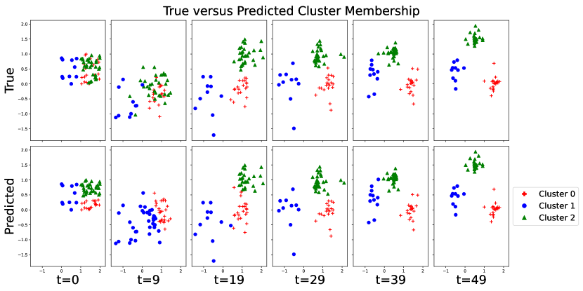
Figure 1: True versus predicted cluster membership of moving clusters. The ground truth contains static clusters, while the predicted clusters are dynamic, allowing points to switch clusters between time steps.

Further, the matrix ${\bf C}$ is used to visualize the paths of the identified dynamic clusters. This ability to directly track clusters is unavailable with any existing spatiotemporal clustering method without extensive post-processing. The top row of Figure 2 shows true versus predicted cluster paths for the same synthetic data as above. We note that the cluster paths are not identified perfectly because the method does not match the data generating mechanism, i.e. we do dynamic prediction on static clusters. Even so, STKM is able to pick up the general trends of cluster movement. This result suggests that even in a dynamic environment, where points are able to change cluster membership, we do not completely lose information about long-term, static cluster behavior.

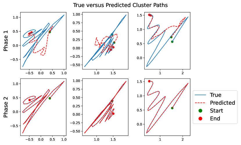
Figure 2: True static versus predicted cluster paths for Phase 1 and Phase 2 of STKM . In Phase 1, STKM identifies general trends of cluster movement, even when allowing points to switch clusters over time. In Phase 2, STKM correctly identifies the true static cluster paths.

One of the drawbacks of building upon $k$-means is that $k$-means is well known to break down in the presence of outliers and noise. In a dataset, such as the one in the top row of Figure 3, we expect outliers to skew cluster centers, and thereby cluster membership significantly. This behavior is exactly what is observed in row two of Figure 3 when applying STKM to a dataset with outliers. The outliers are incorrectly assigned as one cluster and the two ground truth clusters are assigned to one large cluster for the majority of time steps. A possible solution to this problem is to replace the Euclidean distance between points and their cluster centers in Equation 1 with a more robust distance function, such as $log\bigg{(}c+||{\bf x}_{t,i}-{\bf c}_{t,j}||^{2}\bigg{)}$, where $c\geq 1$ is a constant. Doing so allows for the two ground truth clusters to retain their individual identities over all time steps, as seen in row three of Figure 3. Further post-processing to trim those points furthest from their cluster centers could potentially identify outliers as well. Although a robust distance function prevents outliers and noise from corrupting the clustering results, it also adds to run time and scales poorly with problem size. Therefore, for the remainder of the paper, we focus on the standard version of STKM and leave the investigation of robust versions to future work.

Another concern of a $k$-means based approach is handling missing data. The formulation of the objective in Equation 1 requires all points to exist at the same time steps across the entire time span of observation. In order to ensure this criteria is satisfied, data can be divided into time intervals, and data missing spatial information in an interval can be augmented using interpolation, while data with multiple spatial coordinates in an interval can be reduced through averaging.

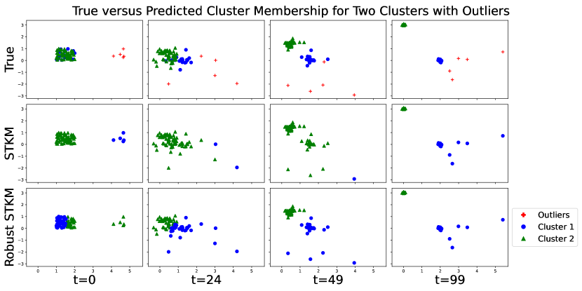
Figure 3: True versus predicted cluster membership for two clusters plus outliers. STKM is unable to produce a good result, while Robust STKM retains the identities of both clusters, even in the presence of noise.

3.2 Phase 2: Stable, Long-term Associations

Phase 2 of STKM aims to identify the stable-long term associations between data points. The output of Phase 2 is a single assignment of static long-term clusters containing points that have the most similar spatiotemporal characteristics. Phase 2 outputs the same information as spatiotemporal clustering methods in the event clustering, geo-referenced data item clustering, and geo-referenced time-series clustering classifications. However, because Phase 2 builds upon Phase 1, taking into account short-term information in making decisions about long-term behavior, the long-term clusters predicted by Phase 2 are more accurate than a method from the aforementioned classifications.

Intuitively, points that have similar cluster assignment histories will travel together in the long run. We can apply Phase 2 to any method that outputs an assignment for each point at every iteration. In order to apply Phase 2 to the output from Phase 1, we first need to extract the cluster assignment histories from the weight matrix ${\bf W}$. We define the cluster assignment histories as in (4), so that ${\bf a}_{i}\in\mathbb{R}^{T}$ is a vector where each entry contains the cluster assignment of point $i$ at time $t$.

$${\bf a}_{i}=\arg\max_{j}{\bf w}_{t,:,i}$$ (4)

Then the cluster assignment similarity measure between two cluster assignment history vectors is simply the magnitude of the intersection of the two vectors over the total number of time steps, as shown in (5).

$$sim({\bf a}_{i},{\bf a}_{j})=\frac{|{\bf a}_{i}\cap{\bf a}_{j}|}{|{\bf a}_{i}|}$$ (5)

Using this similarity measure, we define a cluster assignment similarity matrix ${\bf A}$ where $A_{i,j}$ contains the similarity between point $i$ and point $j$. Given a similarity threshold $\theta$, we can then assign points to static long-term clusters. If we know the number of long-term clusters $k$, we can search for a value of $\theta$ that results in $k$ long-term clusters. The larger the value of $\theta$, the fewer points will be clustered together, and the more clusters will be predicted. Conversely, the smaller the value of $\theta$, the fewer long-term clusters will be output. If there does not exist a value of $\theta$ that produces $k$ long-term clusters, the value of $\theta$ is chosen to be such that as close to $k$ clusters are predicted. Because the output of this procedure depends on the order in which the point assignment histories are processed, we randomly shuffle the rows of ${\bf A}$ and run the procedure five times, choosing the long term clusters that are output the majority of the time. If no set of long-term clusters are output over half of the time, we continue to run the procedure up to 20 times until this condition is satisfied. If after 20 runs, there is no clear majority, we instead choose the long-term set that is output most often.

In row two of Figure 2, we see the result of predicting the static, long-term cluster paths of the moving objects from the previous section. Phase 2 identifies the true, static cluster paths perfectly. By combining the results from Phase 1 and Phase 2, we can form a visualization like the one in Figure 4, where the cluster assignment histories of three points from each long-term cluster are displayed. Now, not only do we know which points behave most similarly in the long-run, we also know the interactions of each individual point at every time step. We are able to gain insights such as, the three points tracked in long-term Clusters $0$ and $1$ spend significant time in the other two clusters, whereas the three points tracked in Cluster $2$ spend the vast majority of their time in Cluster $2$. This analysis provides valuable information about the multi-scale behavior of the moving objects.

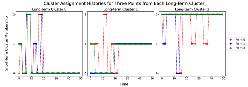
Figure 4: Cluster assignment histories for three points from each long term cluster.

4 Experiments

In order to evaluate the performance of our proposed method, we perform experiments on the spatiotemporal benchmark dataset proposed by Cakmak et. al  [7]. Recognizing that there was no unified and commonly used experimental dataset and protocol in the field of spatiotemporal clustering, Cakmak et. al proposed a benchmark for detecting moving clusters in collective animal behavior. Their benchmark is based on three collective animal behavior models and contains $3,600$ spatiotemporal datasets of sizes ranging from $600$ up to $520,000$, where size is determined by multiplying together number of time steps and number of objects. The datasets track static clusters, where points do not change cluster membership over time  [7]. During our evaluation, we focus on the benchmark datasets that have size between $800$ and $35,000$, of which there are $1,034$. We take this approach, because we are particularly interested in the performance of our method in the low-data domain, where either we have very few objects or very few time steps from which to infer behavior.

Cakmak et. al measure clustering quality with the adjusted mutual information (AMI) score and report execution time for a handful of baseline methods. The implemented baseline methods all allow points to switch clusters between time steps, and the reported AMI compares the full cluster assignment histories against the ground truth, which does not allow for point switching. While this comparison provides a way to evaluate the short-term associations, because of the mismatch between the method and the data generating mechanism, we believe that it is more informative to compare the stable, long-term associations derived from the full assignment histories against the ground truth. Therefore, we report both what refer to as the total AMI for the full cluster assignment histories and the long-term AMI for the long-term associations. We calculate total AMI as in Cakmak et. al by comparing the cluster assignment histories to the ground truth static cluster assignments. We obtain the long-term AMI by applying Phase 2 of our method to both our output from Phase 1 and the cluster assignment histories of the baseline methods. As in  [7], we divide our data into groups based on size (e.g. 800-3000 data points, 3000-6000 points, etc.). We report results as the median and average of total and long-term AMI for each range of dataset sizes.

We note that in  [7], during the cluster merging process, points that cannot be assigned to a cluster are given the same label. This labeling results in an erroneous association of unassigned points as a single cluster during the calculation of AMI. In order to avoid interpreting unassigned points as a single cluster, we ensure that they are all given unique labels when we calculate total and long-term AMI.

All of the baseline methods have at least four parameters that need to be defined: frame size, frame overlap, $\epsilon_{1}$, and $\epsilon_{2}$, which correspond to the number of time steps that belong to a single frame, the number of time steps that frames overlap when associating clusters between frames, and the spatial and temporal distances that define whether a point is density reachable from the current one. In addition, all of the methods except for ST-DBSCAN take as input the true number of clusters $k$. In their experiments, Cakmak et. al arbitrarily fix frame size to be $100$ and frame overlap to be $10$. All of the methods use the default value $\epsilon_{1}=0.50$, except for ST-DBSCAN, which searches for $\epsilon_{1}\in[0.01,0.05]$. Grid search is used in  [7] to find the optimal remaining parameters that achieve the highest accuracy measure against the ground truth. In a true unsupervised setting, ground truth labels are not available, and we cannot tune parameters to maximize our accuracy. We argue that the performance report of the baseline methods in Cakmak et. al is therefore unrealistic and avoid parameter tuning in our experiments.

In contrast, Phase 1 of our method requires only two parameters: $\lambda$, which controls the extent of the penalty that indirectly discourages points from switching clusters, and $k$, the true number of clusters. Since $\lambda$ is confined to the range $[0,1]$, the meaning of its value is intuitive. The same is not true of $\epsilon_{2}$ from the baseline methods. In order to create an intuitive interpretation of $\epsilon_{2}$, we define $\epsilon_{2}=\alpha t$, where $t$ is the total number of time steps in the data and $\alpha\in[0,1]$ is some given proportion. This formulation gives us a principled approach to choosing the temporal distance a point is density reachable from the current one, as opposed to arbitrarily choosing a value for each individual data set.

Because we know that the ground truth clusters do not allow points to switch clusters, we set both $\lambda$ and $\alpha$ fairly high. We run all of the methods on each set of data with $\lambda,\alpha=[0.60,0.80,1.00]$. For the baseline methods, we fix the remaining parameters as follows: frame size $=100$, frame overlap $=10$, $\epsilon_{1}=0.50$ for all of the methods, except for ST-DBSCAN where $\epsilon=0.05$, and $k$ is set to the true number of clusters. Any other parameters in the baseline methods are set to their default values. Since we run each method three times using different parameters on each dataset, we obtain metrics for 3,102 runs of each method. We then report the aggregates of the total and long-term AMI for each method on every range of dataset sizes in Figures 5-7.

5 Results

Figure 5 presents the results for total AMI, which compares full, variable cluster assignment histories against static ground truth clusters, for various methods on differently sized datasets. The trendlines connecting the medians and averages of AMI on each dataset size in 5(a) are shown in orange and blue, respectively. We note that over all dataset sizes, the boxpolots for all methods span the entire range from $0$ to $1$, emphasizing the difficulty of the moving object clustering task that comes from evaluating a method that does not match the data generating mechanism. Figures 5(b) and 5(c) provide a closer look at average and median total AMI score trendlines. STKM achieves the highest average total AMI on datasets of size smaller than $20,000$, but maintains the highest median total AMI over all dataset sizes, showing that although STKM achieves higher total AMI scores more often, those scores are on average smaller in magnitude than those achieved by other methods. The boxplots in Figure 5(a) further emphasize this result. The $25th$ percentiles of the STKM boxplots are all higher than other methods, but the $75th$ percentiles are substantially lower on larger datasets. The observed inverse relationship between full AMI and dataset size is expected, as points have more opportunities to change cluster membership over longer spans of time or in datasets with greater spatial density.

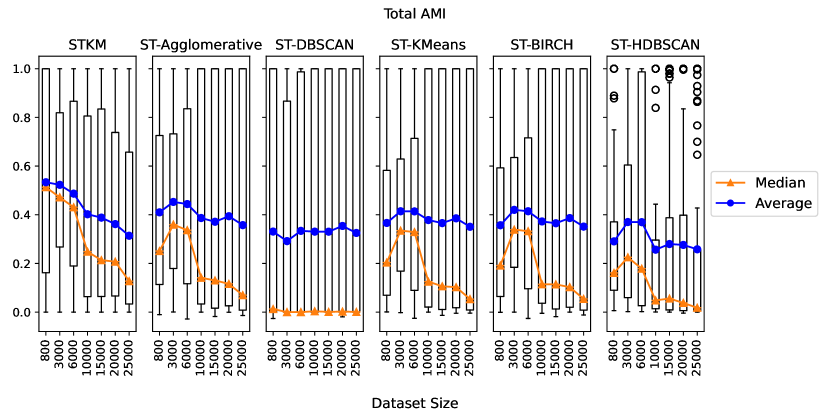
(a)

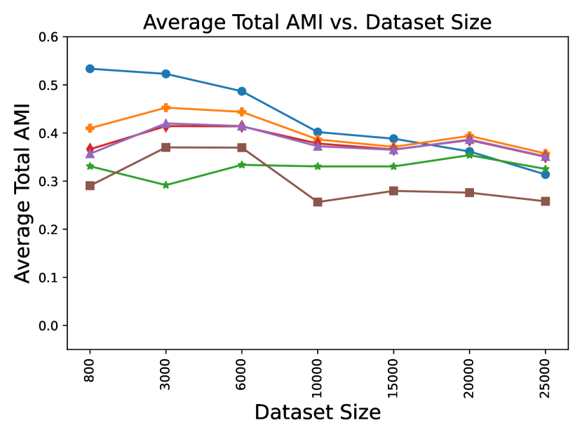
(b)

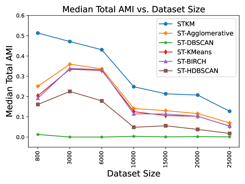
(c)

Figure 5: (a) Boxplots of total AMI scores for various methods over different dataset sizes. Median scores are shown in orange and average scores in blue. (b) A closeup of the average total AMI trendlines. (c) A closeup of the median total AMI trendlines. Boxplots for all methods and dataset sizes span the entire range $[0.0,1.0]$, demonstrating the difficulty of evaluating a method that does not match the data generating mechanism. STKM achieves the highest average total AMI on datasets of size $\leq 20,000$, but maintains the highest median total AMI on all dataset sizes. On larger datasets, STKM scores higher in terms of total AMI more often, even though the magnitude of those scores is smaller.

Recall that long-term AMI, compares predicted static against ground truth static clusters. We intuitively expect objects that spend the most time transiently clustered together to travel in the same long-term clusters. We therefore expect higher total AMI, which scores the accuracy of our transient associations, to correlate with higher long-term AMI, which scores the accuracy of our static associations. However, Figure 6, which show the results of long-term AMI for various methods on differently sized data sets, presents a different story. STKM, ST-Agglomerative, ST-KMeans, and ST-BIRCH score almost identically in terms of their median trendlines, but STKM maintains the highest average long-term AMI over all dataset sizes. Further, the boxplots for STKM in Figure 6(a) have the tightest interquartile ranges, demonstrating that STKM has the lowest variability in terms of long-term AMI scores. This result implies that the short-term relationships that STKM detects are more informative than existing methods in identifying long-term point relationships. Figures 6(b) and 6(c) also include the results of baseline ST-DBSCAN, which is a method in the geo-referenced data item clustering classification that produces static cluster assignments. All of the other methods, which use Phase 2 of STKM to generate static cluster assignments, outperform baseline ST-DBSCAN, suggesting that a two phase approach that uses short-term behavior to inform long-term relationships, is more reliable.

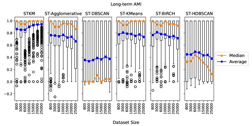
(a)

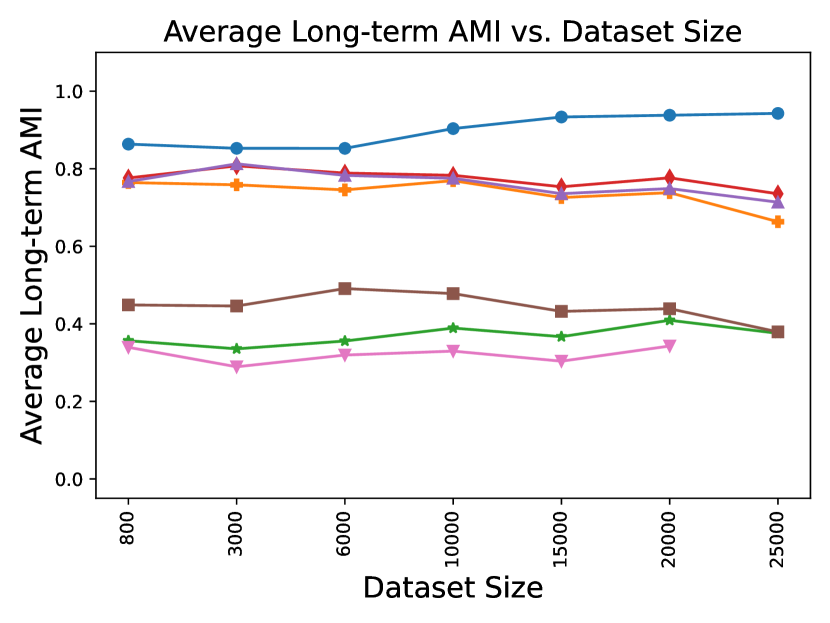
(b)

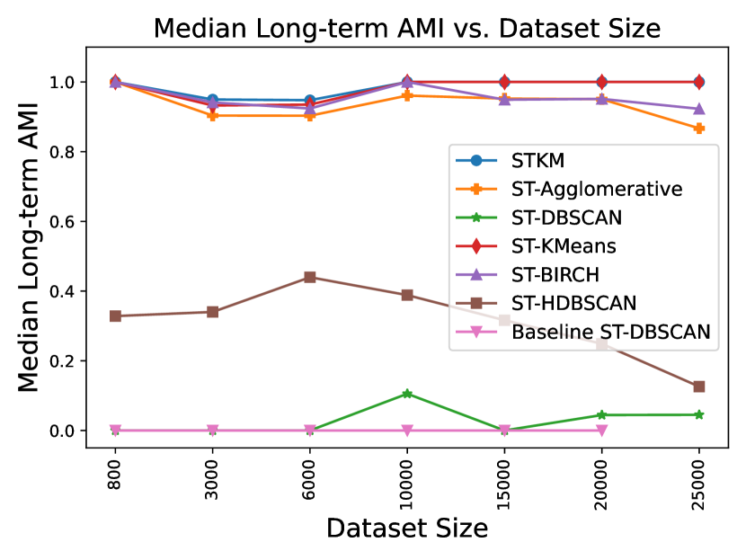
(c)

Figure 6: (a) Boxplots of long-term AMI scores for various methods over different dataset sizes. Median scores are shown in orange and average scores in blue. (b) A closeup of average long-term AMI trendlines. (c) A closeup of median long-term AMI trendlines. Boxplots for STKM have the smallest interquartile ranges, showing STKM’s long-term AMI scores are the least variable. STKM achieves both the highest average and median long-term AMIs on datasets of all sizes. All methods that use short-term information to inform long-term predictions perform better than Baseline ST-DBSCAN, which does not provide information on short-term associations between data points.

When STKM is compared directly against the benchmark methods on a dataset by dataset basis, it achieves the best performance in terms of both total and long-term AMI. STKM scores the highest total AMI on $55\%$ of the data and the highest long-term AMI on $70\%$ of the data. It achieves both the highest total and long-term AMI on $49\%$ of the data. Table 1 shows the average of all total AMI and long-term AMI scores for each of the tested methods over all 3,102 datasets. STKM moderately outperforms the other methods in terms of average total AMI and significantly outperforms the other methods in terms of average long-term AMI, highlighting its superior performance. Although STKM demonstrably outputs more informative moving cluster labels and more accurate long-term cluster labels, the trade-off is it’s runtime. STKM runs slowest of all methods tested, as seen in Figure 7.

	STKM	ST-Agglomerative	ST-DBSCAN	ST-KMeans	ST-BIRCH	ST-HDBSCAN
Average Total AMI	.42	.40	.33	.38	.38	.30
Average Long-term AMI	.90	.73	.37	.77	.76	.44

Table 1: Average Total and Long-term AMIs for all methods over all dataset sizes. STKM achieves the highest scores for both accuracy metrics.

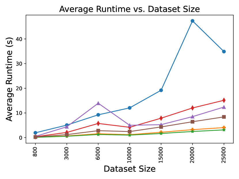
(a)

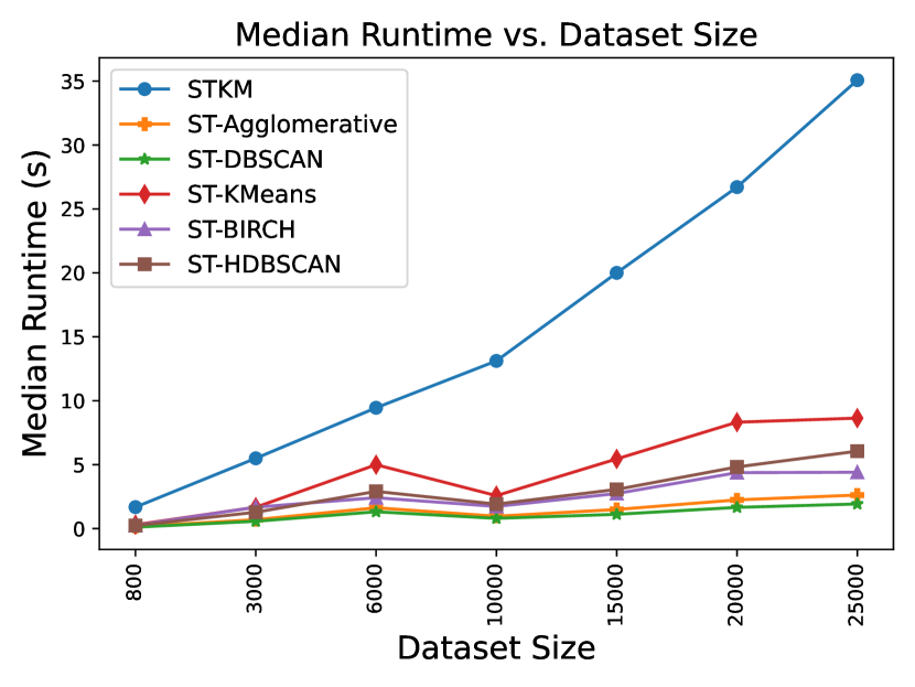
(b)

Figure 7: STKM has the longest runtime of all methods on datasets of all sizes.

6 Conclusion

We demonstrate that STKM, a two phase spatiotemporal clustering method, is able to capture the multi-scale behavior of moving object data. Phase 1 returns an assignment for each point at every iteration, and provides us the unique ability to directly track cluster centers without any post-processing. This phase minimizes an objective function, that unlike existing methods, is unified in both space and time and requires many fewer parameters to run. Phase 2 can be optionally applied to classify each point into a single long-term cluster. Because Phase 2 infers long-term relationships from short-term ones, applying both Phase 1 and Phase 2 results in more accurate predicted static clusters compared to methods that provide exclusively static clusters. The combination of both phases also allows us to explore the individual behavior of points in long-term clusters and draw conclusions about the relationships between clusters.

We demonstrate the competitiveness of STKM against existing spatiotemporal clustering methods on a benchmark dataset proposed by Cakmak et. al  [7]. Our comprehensive comparison evaluates the predicted dynamic clusters against ground-truth static clusters using adjusted mutual information score. We refer to this measure as total AMI. STKM achieves the highest average total AMIs on datasets of size smaller than $20,000$ and the highest median total AMIs on all datasets. Averaging over all data sizes, STKM scores the highest average total AMI of all methods it is compared against. We show that the results of long-term AMI, which compares predicted static against ground-truth static clusters, are more representative of performance. We derive long-term clusters by applying Phase 2 of STKM both to the output of Phase 1 and to the outputs of the baseline methods. We show that STKM performs best in terms of average and median long-term AMI over all datasets, suggesting that the short-term relationships predicted by STKM are more informative than those of other methods. The tradeoff in using STKM is a slower runtime.

Overall, STKM demonstrably outperforms existing methods on the moving cluster problem. In the future, we intend to further explore robust versions of STKM for handling noisy spatiotemporal data as well as approaches to estimating the number of clusters $k$. With ever increasing information from broad applications such as surveillance, transportation, environmental and seismology studies, and mobile data analysis, STKM and other related methods are critical for the unsupervised analysis of spatiotemporal data streams.

References

- [1] KP Agrawal, Sanjay Garg, Shashikant Sharma, and Pinkal Patel. Development and validation of optics based spatio-temporal clustering technique. Information Sciences, 369:388–401, 2016.
- [2] Mohd Yousuf Ansari, Amir Ahmad, Shehroz S Khan, Gopal Bhushan, et al. Spatiotemporal clustering: a review. Artificial Intelligence Review, 53(4):2381–2423, 2020.
- [3] Hédy Attouch, Jérôme Bolte, Patrick Redont, and Antoine Soubeyran. Proximal alternating minimization and projection methods for nonconvex problems: An approach based on the kurdyka-łojasiewicz inequality. Mathematics of operations research, 35(2):438–457, 2010.
- [4] Panthadeep Bhattacharjee and Pinaki Mitra. A survey of density based clustering algorithms. Frontiers of Computer Science, 15(1):1–27, 2021.
- [5] Derya Birant and Alp Kut. St-dbscan: An algorithm for clustering spatial–temporal data. Data & knowledge engineering, 60(1):208–221, 2007.
- [6] Christopher M Bishop and Nasser M Nasrabadi. Pattern recognition and machine learning, volume 4. Springer, 2006.
- [7] Eren Cakmak, Manuel Plank, Daniel S Calovi, Alex Jordan, and Daniel Keim. Spatio-temporal clustering benchmark for collective animal behavior. In Proceedings of the 1st ACM SIGSPATIAL International Workshop on Animal Movement Ecology and Human Mobility, pages 5–8, 2021.
- [8] Xi Chen, James H Faghmous, Ankush Khandelwal, and Vipin Kumar. Clustering dynamic spatio-temporal patterns in the presence of noise and missing data. In Twenty-Fourth International Joint Conference on Artificial Intelligence, 2015.
- [9] Marc Hüsch, Bruno U Schyska, and Lueder von Bremen. Corclustst—correlation-based clustering of big spatio-temporal datasets. Future Generation Computer Systems, 110:610–619, 2020.
- [10] Hesam Izakian, Witold Pedrycz, and Iqbal Jamal. Clustering spatiotemporal data: An augmented fuzzy c-means. IEEE transactions on fuzzy systems, 21(5):855–868, 2012.
- [11] Gareth James, Daniela Witten, Trevor Hastie, and Robert Tibshirani. An introduction to statistical learning, volume 112. Springer, 2013.
- [12] Hoyoung Jeung, Heng Tao Shen, and Xiaofang Zhou. Convoy queries in spatio-temporal databases. In 2008 IEEE 24th International Conference on Data Engineering, pages 1457–1459. IEEE, 2008.
- [13] Panos Kalnis, Nikos Mamoulis, and Spiridon Bakiras. On discovering moving clusters in spatio-temporal data. In International symposium on spatial and temporal databases, pages 364–381. Springer, 2005.
- [14] Zhenhui Li, Bolin Ding, Jiawei Han, and Roland Kays. Swarm: Mining relaxed temporal moving object clusters. Technical report, ILLINOIS UNIV AT URBANA-CHAMPAIGN DEPT OF COMPUTER SCIENCE, 2010.
- [15] Iulian Peca, Georg Fuchs, Katerina Vrotsou, Natalia V Andrienko, and Gennady L Andrienko. Scalable cluster analysis of spatial events. EuroVA@ EuroVis, 6:19–23, 2012.
- [16] Hadi Fanaee Tork. Spatio-temporal clustering methods classification. In Doctoral symposium on informatics engineering, volume 1, pages 199–209. Faculdade de Engenharia da Universidade do Porto Porto, Portugal, 2012.
- [17] Marcos R Vieira, Petko Bakalov, and Vassilis J Tsotras. On-line discovery of flock patterns in spatio-temporal data. In Proceedings of the 17th ACM SIGSPATIAL international conference on advances in geographic information systems, pages 286–295, 2009.
- [18] Xindong Wu, Vipin Kumar, J Ross Quinlan, Joydeep Ghosh, Qiang Yang, Hiroshi Motoda, Geoffrey J McLachlan, Angus Ng, Bing Liu, Philip S Yu, et al. Top 10 algorithms in data mining. Knowledge and information systems, 14(1):1–37, 2008.