Sharp embedding between Wiener amalgam and some classical spaces

Abstract

We establish the sharp conditions for the embedding between Wiener amalgam spaces $W_{p,q}^{s}$ and some classical spaces, including Sobolev spaces $L^{s,r}$, local Hardy spaces $h_{r}$, Besov spaces $B_{p,q}^{s}$, which partially improve and extend the main result obtained by Guo et al. in Guo2017Characterization . In addition, we give the full characterization of inclusion between Wiener amalgam spaces $W_{p,q}$ and $\alpha$-modulation spaces $M_{p,q}^{s,\alpha}$. Especially, at the case of $\alpha=0$ with $M_{p,q}^{s,\alpha}=M_{p,q}^{s}$, we give the sharp conditions of the most general case of these embedding. When $0<p\leqslant 1$, we also establish the sharp embedding between Wiener amalgam spaces and Triebel spaces $F_{p,r}^{s}$.

MSC Classification]42B35, 46E30

1 Introduction

The amalgam spaces decouple the connection between local and global properties. They are first introduced by Norbert Wiener in Wiener1926representation ; Wiener1932Tauberian ; Wiener1959Fourier . The first systematic study has been undertaken by Holland in Holland1975Harmonic . In the 1980s, H.G. Feichtinger in Feichtinger1983Banach ; Feichtinger1990Generalized , described a far-reaching generalization of the Wiener amalgam spaces, where he used $W(B,C)$ to denote the Wiener amalgam spaces with the local component in some Banach spaces $B$ and the global component in some Banach spaces $C$. Feichtinger studied the basic properties of these spaces, including inclusions, duality, complex interpolation, pointwise multiplications, and convolution. The Wiener amalgam spaces $W_{p,q}^{s}$ we talk about here are a class of these spaces, which can be re-expressed as $W({\mathscr{F}^{-1}}L^{q}_{s},L^{p})$.

From another point of view, the Wiener amalgam spaces could be regarded as the Triebel-type space corresponding to the modulation space $M_{p,q}^{s}$. The modulation spaces $M_{p,q}^{s}$ are one of the function spaces introduced by Feichtinger Feichtinger2003Modulation in the 1980s using the short-time Fourier transform to measure the decay and the regularity of the function differently from the usual $L^{p}$ Sobolev spaces or Besov-Triebel spaces. By the frequency-uniform localization technique (Wang2007Frequency ; Cunanan2015Wiener ), Wiener amalgam spaces and modulation spaces could be defined by the uniform decomposition of frequency spaces in contrast with the dyadic decomposition in the definition of Besov-Triebel spaces. Therefore, Wiener amalgam spaces have many properties different from the Besov-Triebel spaces, but similar to modulation spaces. For instance, the Fourier multiplier $e^{i\lvert D\rvert^{\alpha}}(0<\alpha\leqslant 1)$ is unbounded on any classical Lebesgue spaces $L^{p}$ or Besov spaces $B_{p,q}$ with $p\neq 2$, but bounded on all Wiener spaces $W_{p,q}^{s}$ and modulation spaces $M_{p,q}^{s}$. One can see Miyachi1981some ; Guo2020Sharp for more details. Even so, Wiener amalgam spaces have some distinctive properties from modulation spaces.. For example, the Fourier multiplier $e^{i\lvert D\rvert^{\alpha}}(1<\alpha\leqslant 2)$ is unbounded on any modulation spaces $W_{p,q}^{s}$ with $p\neq q$, but bounded on all modulation spaces $M_{p,q}^{s}$. One can refer Benyi2007Unimodular ; Miyachi2009Estimates ; Tomita2010Unimodular ; Chen2012Asymptotic . These Fourier multipliers play a significant role in nonlinear dispersive equations such as nonlinear Schrödinger and wave equations. As a result, it is natural to solve these nonlinear equations in Wiener amalgams and modulation spaces. There are numerous papers about these questions. One can see Wang2007global ; Cordero2008Strichartz ; Cordero2009Remarks ; Benyi2009Local ; Chaichenets2017existence ; Chen2020dissipative ; Oh2020Global ; Bhimani2020Norm .

One basic but important consideration is what these spaces are like embedded in each other, which can tell us how different they are. As for modulation spaces, Wang-Huang in Wang2007Frequency gave the full characterization of the embedding between modulation spaces and Besov spaces. Actually, we can define the $\alpha$-modulation spaces (Borup2006Banach ; Han2014$$ ), which contain modulation spaces with $\alpha=0$ and Besov spaces with $\alpha=1$. Guo et al. in Guo2018Full gave the sharp conditions between the $\alpha$-modulation spaces. Kobayashi and Sugimoto in Kobayashi2011inclusion proved the sharp embedding between Sobolev spaces and modulation spaces. As for Wiener amalgam spaces, Cunanan et al. in Cunanan2015Inclusion gave some necessary and sufficiency conditions for the inclusion relation between $W_{p,q}^{s}$ and $L^{p}$. Later their results were completely extended by Guo et al. in Guo2017Characterization . Guo et al. characterized the embedding between $W_{p,q}^{s}$ and $X$, where $X\in\left\{B_{p,q},L^{p},h_{p}\right\}$ by a mild characterization of the embedding between Triebel and Wiener amalgam spaces.

In this paper, we consider the more general embeddings between $W_{p,q}^{s}$ and $X$, where $X\in\left\{B_{p_{0},q_{0}},L^{r},h_{r},F_{p,q_{0}},M_{p_{0},q_{0}},M_{p,q}^{s,\alpha}\right\}$. Here $(p_{0},q_{0},r)$ could not be equal to $(p,q,p).$

For $a,b\in{\mathbb{R}}$, denote $a\vee b=\min\left\{a,b\right\},a\wedge b=\max\left\{a,b\right\}$. For $0<p,q\leqslant\infty,d\in{\mathbb{N}}$, we denote

$$\tau_{1}(p,q) :=d\left(0\vee(\frac{1}{q}-\frac{1}{2})\vee(\frac{1}{q}+\frac{1}{p}-1)\right)\mathchar 24635\relax\;$$

$$\sigma_{1}(p,q) :=d\left(0\wedge(\frac{1}{q}-\frac{1}{2})\wedge(\frac{1}{q}+\frac{1}{p}-1)\right).$$

As shown in Figure 1 and 2, we have

$$\tau_{1}(p,q)=\begin{cases*}0,&if $(1/p,1/q)\in(1)$;\\ d(1/q-1/2),&if $(1/p,1/q)\in(2)\mathchar 24635\relax\;$\\ d(1/p+1/q-1),&if $(1/p,1/q)\in(3).$\end{cases*}$$

$$\sigma_{1}(p,q)=\begin{cases*}0,&if $(1/p,1/q)\in(1)$;\\ d(1/q-1/2),&if $(1/p,1/q)\in(2)\mathchar 24635\relax\;$\\ d(1/p+1/q-1),&if $(1/p,1/q)\in(3).$\end{cases*}$$

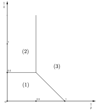
Figure 1: The index sets for $\tau_{1}(p,q)$

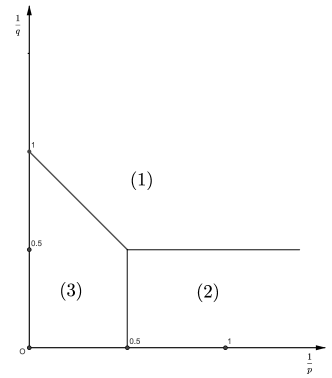
Figure 2: The index sets for $\sigma_{1}(p,q)$

We first consider the sharp embedding between Sobolev spaces $L^{s,r}$ and Wiener amalgam spaces $W_{p,q}$, which is, in some sense, a generalization of the inclusion relation given in Guo2017Characterization . Our main results are as follows.

Theorem 1.

Let $1\leqslant p,r\leqslant\infty,0<q\leqslant\infty,s\in{\mathbb{R}}$. Then $L^{s,r}\hookrightarrow W_{p,q}$ if and only if $r\leqslant p$ and one of the following conditions is satisfied.

(1)

$r>q,q<2,s>\tau_{1}(r,q)\mathchar 24635\relax\;$

(2)

$1<r,2\wedge r\leqslant q,s\geqslant\tau_{1}(r,q)\mathchar 24635\relax\;$

(3)

$r=1,q=\infty,s\geqslant\tau_{1}(r,q)\mathchar 24635\relax\;$

(4)

$r=1,q<\infty,s>\tau_{1}(r,q)$.

Remark 1.

For visualization, one can see Figure 3. Note that the domains divided by the solid lines are corresponding to the conditions in Theorem 1. The following figures of this paper also follow this rule.

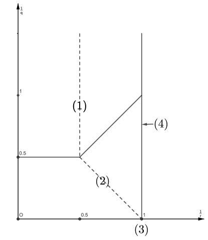
Figure 3: The index sets of Theorem 1

Similarly, we also have

Theorem 2.

Let $1\leqslant p,r\leqslant\infty,0<q\leqslant\infty,s\in{\mathbb{R}}$. Then $W_{p,q}\hookrightarrow L^{s,r}$ if and only if $p\leqslant r$ and one of the following conditions is satisfied.

(1)

$r<q,q>2,s<\sigma_{1}(r,q)\mathchar 24635\relax\;$

(2)

$r<\infty,q\leqslant r\vee 2,s\leqslant\sigma_{1}(r,q)\mathchar 24635\relax\;$

(3)

$r=\infty,0<q\leqslant 1,s\leqslant\sigma_{1}(r,q)\mathchar 24635\relax\;$

(4)

$r=\infty,1<q\leqslant\infty,s<\sigma_{1}(r,q).$

As for the local Hardy space $h_{r}$, our main results are as follows.

Theorem 3.

Let $0<r<\infty$, $0<p,q\leqslant\infty,s\in{\mathbb{R}}$. Then $h_{r}\hookrightarrow W_{p,q}^{-s}$ if and only if $r\leqslant p$ and one of the following conditions is satisfied.

(1)

$r>q,2>q,s>\tau_{1}(r,q)\mathchar 24635\relax\;$

(2)

$r\leqslant q$ or $2\leqslant q,s\geqslant\tau_{1}(r,q).$

Theorem 4.

Let $0<r<\infty,0<p,q\leqslant\infty,s\in{\mathbb{R}}$. Then $W_{p,q}^{-s}\hookrightarrow h_{r}$ if and only if $p\leqslant r$ and one of the following conditions is satisfied.

(1)

$r<q,2<q,s<\sigma_{1}(r,q)\mathchar 24635\relax\;$

(2)

$r\geqslant q$ or $2\geqslant q,s\leqslant\sigma_{1}(r,q).$

As for the Besov spaces $B_{p,q}^{s}$, our main results are as follows.

Theorem 5.

Let $0<p,p_{0},q\leqslant\infty,s\in{\mathbb{R}}$. Then $B_{p_{0},q}^{s}\hookrightarrow W_{p,q}$ if and only if $p_{0}\leqslant p$ and one of the following conditions is satisfied.

(1)

$p\geqslant q,s\geqslant\tau_{1}(p_{0},q)\mathchar 24635\relax\;$

(2)

$p<q,s>\tau_{1}(p_{0},q).$

For visualization, one can see Figure 4.

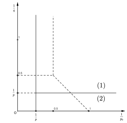
Figure 4: The index sets of Theorem 5

Theorem 6.

Let $0<p,q,p_{0}\leqslant\infty,s\in{\mathbb{R}}$. Then $W_{p,q}\hookrightarrow B_{p_{0},q}^{s}$ if and only if $p\leqslant p_{0}$ and one of the following conditions is satisfied.

(1)

$p\leqslant q,s\leqslant\sigma_{1}(p_{0},q)\mathchar 24635\relax\;$

(2)

$p>q,s<\sigma_{1}(p_{0},q).$

Theorem 7.

Let $0<p,q\leqslant\infty,s\in{\mathbb{R}}$. Moreover, we assume $q\geqslant q_{0}\wedge 2$ or $p\leqslant q_{0}\vee 2$. Then $B_{p,q_{0}}^{s}\hookrightarrow W_{p,q}$ if and only one of the following conditions is satisfied.

(1)

$q_{0}\leqslant p\wedge q,s\geqslant\tau_{1}(p,q)\mathchar 24635\relax\;$

(2)

$p<q_{0}\leqslant q,s>\tau_{1}(p,q)\mathchar 24635\relax\;$

(3)

$q<q_{0},s>\tau_{1}(p,q).$

Theorem 8.

Let $0<p,q\leqslant\infty,s\in{\mathbb{R}}$. Moreover, we assume $q\leqslant q_{0}\vee 2$ or $p\geqslant q_{0}\wedge 2$. Then $W_{p,q}\hookrightarrow B_{p,q_{0}}^{s}$ if and only if one of the following conditions is satisfied.

(1)

$q_{0}\geqslant p\vee q,s\leqslant\sigma_{1}(p,q)\mathchar 24635\relax\;$

(2)

$p>q_{0}\geqslant q,s<\sigma_{1}(p,q)\mathchar 24635\relax\;$

(3)

$q>q_{0},s<\sigma_{1}(p,q).$

As for the modulation spaces $M_{p,q}^{s}$, our main results are as follows.

Theorem 9.

Let $0<p,p_{1},q,q_{1}\leqslant\infty,s\in{\mathbb{R}}$, then $M_{p_{1},q_{1}}^{s}\hookrightarrow W_{p,q}$ if and only if $p_{1}\leqslant p$ and one of the following conditions is satisfied.

(1)

$q_{1}\leqslant p\wedge q,s\geqslant 0\mathchar 24635\relax\;$

(2)

$q_{1}>p\wedge q,s+d/q_{1}>d/(p\wedge q)$.

By dual, we also have

Theorem 10.

Let $0<p,p_{1},q,q_{1}\leqslant\infty,s\in{\mathbb{R}}$, then $W_{p,q}\hookrightarrow M_{p_{1},q_{1}}^{s}$ if and only if $p_{1}\geqslant p$ and one of the following conditions is satisfied.

(1)

$q_{1}\geqslant p\vee q,s\leqslant 0\mathchar 24635\relax\;$

(2)

$q_{1}<p\vee q,s+d/q_{1}<d/(p\vee q)$.

As for $\alpha$-modulation spaces $M_{p,q}^{s,\alpha}$, our main results are as follows.

Theorem 11.

Let $0<p,q\leqslant\infty,s\in{\mathbb{R}},\alpha\in(0,1)$. Then $M_{p,q}^{s,\alpha}\hookrightarrow W_{p,q}$ if and only if one of the following conditions is satisfied.

(1)

$p\geqslant q,s\geqslant\alpha\tau_{1}(p,q)\mathchar 24635\relax\;$

(2)

$p<q,s>\alpha\tau(p,q)+d(1-\alpha)(1/p-1/q).$

For visualization, one can see Figure 5.

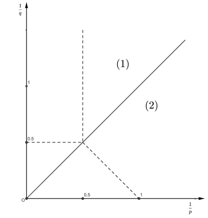
Figure 5: The index sets of Theorem 11

On the other hand, we also have

Theorem 12.

Let $0<p,q\leqslant\infty,s\in{\mathbb{R}},\alpha\in(0,1)$. Then $W_{p,q}\hookrightarrow M_{p,q}^{s,\alpha}$ if and only if one of the following conditions is satisfied.

(1)

$p\leqslant q,s\leqslant\alpha\sigma_{1}(p,q)\mathchar 24635\relax\;$

(2)

$p>q,s<\alpha\sigma_{1}(p,q)+d(1-\alpha)(1/p-1/q).$

For visualization, one can see Figure 6.

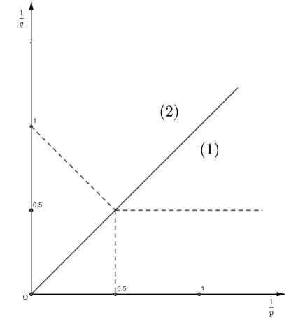
Figure 6: The index sets of Theorem 12

Remark 2.

One can see that when $\alpha=0$, $M_{p,q}^{s,\alpha}=M_{p,q}^{s}$. When $\alpha=1,M_{p,q}^{s,\alpha}=B_{p,q}^{s}$ (see Han2014$$ ). The theorems above coincide with Theorem 5 and 9. But by results in Guo2016Sharpness , we can not only use complex interpolation with $\alpha=0,1$ to get the results for $\alpha\in(0,1)$ as desired.

As for Triebel spaces $F_{p,q}^{s}$ with $0<p\leqslant 1$, our main results are as follows.

Theorem 13.

Let $0<p\leqslant 1,0<q,r\leqslant\infty$, the embedding $F_{p,r}^{s}\hookrightarrow W_{p,q}$ is true if and only if one of the following conditions is satisfied.

(1)

$p\leqslant q,s\geqslant d\left(1/p+1/q-1\right)\mathchar 24635\relax\;$

(2)

$p>q,s>d\left(1/p+1/q-1\right)$.

On the other hand, we have

Theorem 14.

Let $0<p\leqslant 1,0<q,r\leqslant\infty$, we assume $q\leqslant 2$. Then the embedding $W_{p,q}\hookrightarrow F_{p,r}^{s}$ is true if and only if one of the following conditions is satisfied.

(1)

$p\geqslant q,q\leqslant r,s\leqslant 0\mathchar 24635\relax\;$

(2)

$p\geqslant q,q>r,s<0\mathchar 24635\relax\;$

(3)

$p<q,q\leqslant 2,q\leqslant r,s\leqslant 0\mathchar 24635\relax\;$

(4)

$p<q,q\leqslant 2,q>r,s<0.$

The paper is organized as follows. In Section 2, we will give some basic notation. The definitions and some basic properties of the function spaces mentioned above also be contained there. The proofs of our main results will be given in Section 3-9.

2 Preliminaries

2.1 Notation

We write $\mathscr{S}({\mathbb{R}}^{d})$ to denote the Schwartz space of all complex-valued rapidly decreasing infinity differentiable functions on ${\mathbb{R}}^{d}$, and $\mathscr{S}^{\prime}({\mathbb{R}}^{d})$ to denote the dual space of $\mathscr{S}({\mathbb{R}}^{d})$, all called the space of all tempered distributions. For simplification, we omit ${\mathbb{R}}^{d}$ without causing ambiguity. The Fourier transform is defined by ${\mathscr{F}}f(\xi)=\hat{f}(\xi)=\int_{{\mathbb{R}}^{d}}f(x)e^{-ix\xi}d\xi$, and the inverse Fourier transform by ${\mathscr{F}^{-1}}f(x)=(2\pi)^{-d}\int_{{\mathbb{R}}^{d}}f(\xi)e^{ix\xi}d\xi$.

We use the notation $I\lesssim J$ if there is an independently constant C such that $I\leqslant CJ$. Also we denote $I\approx J$ if $I\lesssim J$ and $J\lesssim I$. For $1\leqslant p\leqslant\infty$, we denote the dual index $p^{\prime}$ with $1/p+1/p^{\prime}=1$, for $0<p<1$, denote $p^{\prime}=\infty$. For $0<p,q\leqslant\infty,d\in{\mathbb{N}}$, we also denote

$$a(p,q) :=d(1/p+1/q-1)\mathchar 24635\relax\;$$

$$\tau(p,q) :=d\left(0\vee(\frac{1}{q}-\frac{1}{p})\vee(\frac{1}{q}+\frac{1}{p}-1)\right)\mathchar 24635\relax\;$$

$$\sigma(p,q) :=d\left(0\wedge(\frac{1}{q}-\frac{1}{p})\wedge(\frac{1}{q}+\frac{1}{p}-1)\right).$$

These indexes play a great role in the embedding between modulation spaces and Besov spaces (Wang2007Frequency ).

2.2 Sobolev and local Hardy spaces

For $0<p<\infty$, we define the $L^{p}$ norm:

$$\left\|f\right\|_{p}=\left(\int_{{\mathbb{R}}^{d}}\lvert f(x)\rvert^{p}dx\right)^{1/p}$$

and $\left\|f\right\|_{\infty}=\operatorname*{ess\,sup}_{x\in{\mathbb{R}}^{d}}\lvert f(x)\rvert$. We also define the $L^{p}$ Sobolev norm :

$$\left\|f\right\|_{L^{s,p}}=\left\|(I-\triangle)^{s/2}f\right\|_{p},$$

where $(I-\triangle)^{s/2}={\mathscr{F}^{-1}}(1+\lvert\xi\rvert^{2})^{s/2}{\mathscr{F}}$ is the Bessel potential. Recall that the Sobolev spaces is defined by $L^{s,p}=\left\{f\in\mathscr{S}^{\prime}:\left\|f\right\|_{L^{s,p}}<\infty\right\}$. For more details, One can see Grafakos2009Modern .

Next, we turn to introduce the local Hardy space of Goldberg Goldberg1979local . Let $\psi\in\mathscr{S}$ with $\int_{{\mathbb{R}}^{d}}\psi(x)dx\neq 0$. Denote $\psi_{t}(x)=t^{-d}\psi(t^{-1}x)$. Let $0<p<\infty$, the local Hardy spaces is defined by

$$h_{p}:=\left\{f\in\mathscr{S}^{\prime}:\left\|f\right\|_{h_{p}}=\left\|\sup_{0<t<1}\lvert\psi_{t}*f\rvert\right\|_{p}<\infty\right\}.$$

Similarly, we can define $h_{p}^{s}:=\left\{f\in\mathscr{S}^{\prime}:\left\|(I-\triangle)^{s/2}f\right\|_{h_{p}}<\infty\right\}$. We note that the definition of the local Hardy spaces is independent of the choice of $\psi\in\mathscr{S}$. The local Hardy spaces could also be defined by $h_{p}$-atom. One can refer Triebel1992Theory .

2.3 Modulation and Wiener amalgam spaces

Let $0<p,q\leqslant\infty,s\in{\mathbb{R}}$, the short time Fourier transform (STFT) of $f$ respect to a window function $g\in\mathscr{S}$ is defined as (see Feichtinger2003Modulation ; Groechenig2001Foundations ):

$$V_{g}f(x,\xi)=\int_{{\mathbb{R}}^{d}}f(t)\overline{g(t-x)}e^{-it\xi}dt.$$

We denote

$$\left\|f\right\|_{M_{p,q}^{s}} =\left\|V_{g}f(x,\xi)\left\langle\xi\right\rangle^{s}\right\|_{L_{\xi}^{q}L_{x}^{p}},$$

$$\left\|f\right\|_{W_{p,q}^{s}} =\left\|V_{g}f(x,\xi)\left\langle\xi\right\rangle^{s}\right\|_{L_{x}^{p}L_{\xi}^{q}},$$

where $\left\langle\xi\right\rangle=(1+\lvert\xi\rvert^{2})^{1/2}$.

Modulation space $M_{p,q}^{s}$ are defined as the space of all tempered distribution $f\in\mathscr{S}^{\prime}$ for which $\left\|f\right\|_{M_{p,q}^{s}}$ is finite. Wiener space $W_{p,q}^{s}$ are defined as the space of all tempered distribution $f\in\mathscr{S}^{\prime}$ for which $\left\|f\right\|_{W_{p,q}^{s}}$ is finite.

Also, we know another equivalent definition of modulation spaces and Wiener spaces by uniform decomposition of frequency space (see Groechenig2001Foundations ; Cunanan2015Wiener ).

Let $\sigma$ be a smooth cut-off function adapted to the unit cube $[-1/2,1/2]^{d}$ and $\sigma=0$ outside the cube $[-3/4,3/4]^{d}$, we write $\sigma_{k}=\sigma(\cdot-k)$, and assume that

$$\sum_{k\in{\mathbb{Z}}^{d}}\sigma_{k}(\xi)\equiv 1,\ \forall\xi\in{\mathbb{R}}^{d}.$$

Denote $\sigma_{k}(\xi)=\sigma(\xi-k)$, and $\Box_{k}={\mathscr{F}^{-1}}\sigma_{k}{\mathscr{F}}$, then we have the following equivalent norm of modulation space and Wiener spaces:

$$\left\|f\right\|_{M_{p,q}^{s}} =\left\|\left\langle k\right\rangle^{s}\left\|\Box_{k}f\right\|_{L_{x}^{p}}\right\|_{\ell_{k\in{\mathbb{Z}}^{d}}^{q}},$$

$$\left\|f\right\|_{W_{p,q}^{s}} =\left\|\left\|\left\langle k\right\rangle^{s}\Box_{k}f\right\|_{\ell_{k\in{\mathbb{Z}}^{d}}^{q}}\right\|_{L_{x}^{p}}.$$

For simplicity, we denote $X_{p,q}^{s}$ to represent $M_{p,q}^{s}$ or $W_{p,q}^{s}$ below. We simply write $X_{p,q}$ instead of $X_{p,q}^{0}$. One can prove the $X_{p,q}^{s}$ norm is independent of the choice of cut-off function $\sigma$. Also $X_{p,q}^{s}$ is a quasi Banach space and when $1\leqslant p,q\leqslant\infty$, $X_{p,q}^{s}$ is a Banach space. When $p,q<\infty$, then $\mathscr{S}$ is dense in $X_{p,q}^{s}$. Also, $X_{p,q}^{s}$ has some basic properties, we list them in the following lemma (see Wang2007Frequency ; Wang2011Harmonic ; Cunanan2015Wiener ; Groechenig2001Foundations ).

Lemma 15.

Let $s,s_{0},s_{1},\in{\mathbb{R}},0<p,p_{0},p_{1},q,q_{0},q_{1}\leqslant\infty$.

(1)

If $s_{0}\leqslant s_{1},p_{1}\leqslant p_{0},q_{1}\leqslant q_{0}$, we have $X_{p_{1},q_{1}}^{s_{1}}\hookrightarrow X_{p_{0},q_{0}}^{s_{0}}$.

(2)

When $p,q<\infty$, the dual space of $X_{p,q}^{s}$ is $X_{p^{\prime},q^{\prime}}^{-s}$.

(3)

The interpolation spaces theorem is true for $X_{p,q}^{s}$, i.e. for $0<\theta<1$ when

$$s=(1-\theta)s_{0}+\theta s_{1},\quad\frac{1}{p}=\frac{1-\theta}{p_{0}}+\frac{\theta}{p_{1}},\quad\frac{1}{q}=\frac{1-\theta}{q_{0}}+\frac{\theta}{q_{1}},$$

we have $\left(X_{p_{0},q_{0}}^{s_{0}},X_{p_{1},q_{1}}^{s_{1}}\right)_{\theta}=X_{p,q}^{s}$.

(4)

When $q_{1}<q,s+d/q>s_{1}+d/q_{1}$, then we have $X_{p,q}^{s}\hookrightarrow X_{p,q_{1}}^{s_{1}}$.

(5)

When $p\geqslant q,M_{p,q}^{s}\hookrightarrow W_{p,q}^{s}$. When $p\leqslant q,W_{p,q}^{s}\hookrightarrow M_{p,q}^{s}$.

Lemma 16 (Ruzhansky2011Changes ).

Let $0<p,q\leqslant\infty$, and $f\in\mathscr{S}^{\prime}$ with support in $B(0,1)$. Then $f\in M_{p,q}$ is equivalent to $f\in{\mathscr{F}}L^{q}$, is also equivalent to $f\in W_{p,q}$. Moreover, we have

$$\left\|f\right\|_{M_{p,q}}\approx\left\|f\right\|_{W_{p,q}}\approx\left\|f\right\|_{{\mathscr{F}}L^{q}}.$$

2.4 Besov-Triebel spaces

Let $0<p,q\leqslant\infty,s\in{\mathbb{R}},$ choose $\psi:{\mathbb{R}}^{d}\rightarrow[0,1]$ be a smooth radial bump function adapted to the ball $B(0,2)$: $\psi(\xi)=1$ as $\lvert\xi\rvert\leqslant 1$ and $\psi(\xi)=0$ as $\lvert\xi\rvert\geqslant 2$. We denote $\varphi(\xi)=\psi(\xi)-\psi(2\xi)$, and $\varphi_{j}(\xi)=\varphi(2^{-j}\xi)$ for $1\leqslant j,j\in{\mathbb{Z}}$, $\varphi_{0}(\xi)=1-\sum_{j\geqslant 1}\varphi_{j}(\xi)$. Denote $\triangle_{j}={\mathscr{F}^{-1}}\varphi_{j}{\mathscr{F}}$. We say that $\left\{\triangle_{j}\right\}_{j\geqslant 0}$ are the dyadic decomposition operators. The Besov spaces $B_{p,q}^{s}$ and the Triebel spaces $F_{p,q}^{s}$ are defined in the following way :

$$B_{p,q}^{s}=\left\{f\in\mathscr{S}^{\prime}({\mathbb{R}}^{d}):\left\|f\right\|_{B_{p,q}^{s}}=\left\|2^{js}\left\|\triangle_{j}f\right\|_{L_{x}^{p}}\right\|_{\ell_{j\geqslant 0}^{q}}<\infty\right\},$$

$$F_{p,q}^{s}=\left\{f\in\mathscr{S}^{\prime}({\mathbb{R}}^{d}):\left\|f\right\|_{F_{p,q}^{s}}=\left\|\left\|2^{js}\triangle_{j}f\right\|_{\ell_{j\geqslant 0}^{q}}\right\|_{L_{x}^{p}}<\infty\right\}.$$

One can prove that the Besov-Triebel norms defined by different dyadic decompositions are all equivalent (see Triebel1992Theory ), so without loss of generality, we can assume that when $1\leqslant j$, $\varphi_{j}(\xi)=1$ on $D_{j}:=\left\{\xi\in{\mathbb{R}}^{d}:\frac{3}{4}2^{j}\leqslant\lvert\xi\rvert\leqslant\frac{5}{4}2^{j}\right\}$ for convenience. Also, Besov-Triebel spaces have some basic properties known already (see Triebel1992Theory ).

Lemma 17.

Let $s,s_{1},s_{2}\in{\mathbb{R}},0<p,p_{1},p_{2},q,q_{1},q_{2}\leqslant\infty$.

(1)

If $q_{1}\leqslant q_{2}$, we have $B_{p,q_{1}}^{s}\hookrightarrow B_{p,q_{2}}^{s}$, $F_{p,q_{1}}^{s}\hookrightarrow F_{p,q_{2}}^{s}$.

(2)

$\forall\varepsilon>0$, we have $B_{p,q_{1}}^{s+\varepsilon}\hookrightarrow B_{p,q_{2}}^{s}$, $F_{p,q_{1}}^{s+\varepsilon}\hookrightarrow F_{p,q_{2}}^{s}$.

(3)

$B_{p,p\wedge q}^{s}\hookrightarrow F_{p,q}^{s}\hookrightarrow B_{p,p\vee q}^{s}$.

(4)

If $p_{1}\leqslant p_{2},s_{1}-d/p_{1}=s_{2}-d/p_{2}$, we have $B_{p_{1},q}^{s_{1}}\hookrightarrow B_{p_{2},q}^{s_{2}}$.

(5)

If $p_{1}<p_{2},s_{1}-d/p_{1}=s_{2}-d/p_{2}$, we have $F_{p_{1},q_{1}}^{s_{1}}\hookrightarrow F_{p_{2},q_{2}}^{s_{2}}$.

(6)

When $1\leqslant p,q<\infty$, the dual space of $B_{p,q}^{s}$ is $B_{p^{\prime},q^{\prime}}^{-s}$, the dual space of $F_{p,q}^{s}$ is $F_{p^{\prime},q^{\prime}}^{-s}$.

(7)

The interpolation spaces theorem is true for $B_{p,q}^{s}$ and $F_{p,q}^{s}$, i.e. for $0<\theta<1$ when

$$s=(1-\theta)s_{0}+\theta s_{1},\quad\frac{1}{p}=\frac{1-\theta}{p_{0}}+\frac{\theta}{p_{1}},\quad\frac{1}{q}=\frac{1-\theta}{q_{0}}+\frac{\theta}{q_{1}},$$

we have $\left(B_{p_{0},q_{0}}^{s_{0}},B_{p_{1},q_{1}}^{s_{1}}\right)_{\theta}=B_{p,q}^{s}$, $\left(F_{p_{0},q_{0}}^{s_{0}},F_{p_{1},q_{1}}^{s_{1}}\right)_{\theta}=F_{p,q}^{s}.$

(8)

When $0<p<\infty$, we have $F_{p,2}^{s}=h_{p}^{s}$, when $1<p<\infty$, $F_{p,2}^{s}=L^{s,p}$.

2.5 $\alpha$-modulation spaces

Definition 1 ($\alpha$-covering).

A countable set $\left\{Q_{i}\right\}_{i}$, where $Q_{i}\subseteq{\mathbb{R}}^{d}$, is called a $\alpha$-covering of ${\mathbb{R}}^{d}$ if:

(i)

${\mathbb{R}}^{d}=\cup_{i}Q_{i}$,

(ii)

$\#\left\{Q^{\prime}\in Q_{i}:Q^{\prime}\cap Q\neq\emptyset\right\}\leqslant c(d),$ uniformly for $Q\in Q_{i}$,

(iii)

$\left\langle x\right\rangle^{\alpha d}\approx\lvert Q_{i}\rvert$ uniformly for $x\in Q_{i}$.

Definition 2 ($\alpha$-Modulation spaces, Han2014$$ ).

Let $\alpha<1$, denote $\alpha=\alpha/(1-\alpha)$, suppose that $C>c>0$ are two appropriate constants such that $\left\{B_{k}\right\}_{k\in{\mathbb{Z}}^{d}}$ is a $\alpha$-covering of ${\mathbb{R}}^{d}$, where $B_{k}=B(\left\langle k\right\rangle^{\alpha}k,\left\langle k\right\rangle^{\alpha})$. We can choose a Schwartz function sequence $\left\{\eta_{k}^{\alpha}\right\}_{k\in{\mathbb{Z}}^{d}}$ satisfying

$$\begin{cases*}\lvert\eta_{k}^{\alpha}(\xi)\rvert\gtrsim 1,\ \mbox{ if }\lvert\xi-\left\langle k\right\rangle^{\frac{\alpha}{1-\alpha}}k\rvert<c\left\langle k\right\rangle^{\frac{\alpha}{1-\alpha}}\mathchar 24635\relax\;\\ {\mbox{supp}\ }\eta_{k}^{\alpha}\subseteq\left\{\xi:\lvert\xi-\left\langle k\right\rangle^{\frac{\alpha}{1-\alpha}}k\rvert<C\left\langle k\right\rangle^{\frac{\alpha}{1-\alpha}}\right\}\mathchar 24635\relax\;\\ \sum_{k\in{\mathbb{Z}}^{d}}\eta_{k}^{\alpha}(\xi)\equiv 1,\ \forall\xi\in{\mathbb{R}}^{d}\mathchar 24635\relax\;\\ \lvert\partial^{\gamma}\eta_{k}^{\alpha}(\xi)\rvert\leqslant C_{\alpha}\left\langle k\right\rangle^{-\frac{\alpha\lvert\gamma\rvert}{1-\alpha}},\ \forall\xi\in{\mathbb{R}}^{d},\gamma\in{\mathbb{N}}^{d},\end{cases*}$$

where $C_{\alpha}$ is a positive constant depending only on $d$ and $\alpha$. We usually call these $\left\{\eta_{k}^{\alpha}\right\}_{k\in{\mathbb{Z}}^{d}}$ the bounded admission partition of unity corresponding ($\alpha-$ BAPU) to the $\alpha$-covering $\left\{B_{k}\right\}_{k\in{\mathbb{Z}}^{d}}$. The frequency decomposition operators can be defined by

$$\Box_{k}^{\alpha}:={\mathscr{F}^{-1}}\eta_{k}^{\alpha}{\mathscr{F}}.$$

Let $1\leqslant p,q\leqslant\infty,s\in{\mathbb{R}},\alpha\in[0,1)$, the $\alpha$-modulation space is defined by

$$M_{p,q}^{s,\alpha}=\left\{f\in\mathscr{S}^{\prime}:\left\|f\right\|_{M_{p,q}^{s,\alpha}}=\left(\sum_{k\in{\mathbb{Z}}^{d}}\left\langle k\right\rangle^{sq/(1-\alpha)}\left\|\Box_{k}^{\alpha}f\right\|_{p}^{q}\right)^{1/q}<\infty\right\},$$

with the usual modification when $q=\infty$.

When $\alpha=0$, we usually denote $M_{p,q}^{s,\alpha}$ by $M_{p,q}^{s}$. $M_{p,q}^{s,\alpha}$ have some basic properties as follows. One can find their proofs in Han2014$$ .

Lemma 18.

Let $0<p\leqslant\infty,0<q,q_{1}\leqslant\infty,s,s_{1}\in{\mathbb{R}},\alpha\in(0,1)$. Then we have

(1)

if $s\geqslant 0$, $q_{1}\geqslant q$, then $M_{p,q}^{s,\alpha}\hookrightarrow M_{p,q_{1}}^{0,\alpha}$;

(2)

if $q>q_{1},s>d(1-\alpha)(1/q_{1}-1/q)$, then $M_{p,q}^{s,\alpha}\hookrightarrow M_{p,q_{1}}^{0,\alpha}.$

The sharp embeddings between $M_{p,q}^{s,\alpha}$ have been proved before. One can refer Han2014$$ and Guo2018Full .

Lemma 19.

Let $0<p,q\leqslant\infty,s\in{\mathbb{R}},\alpha\in(0,1)$. Then

(1)

$M_{p,q}^{s,\alpha}\hookrightarrow M_{p,q}$ if and only if $s\geqslant\alpha\tau(p,q)$.

(2)

$M_{p,q}\hookrightarrow M_{p,q}^{s,\alpha}$ if and only if $s\leqslant\alpha\sigma(p,q).$

(3)

$B_{p,q}^{s}\hookrightarrow M_{p,q}^{0,\alpha}$ if and only if $s\geqslant(1-\alpha)\tau(p,q).$

(4)

$M_{p,q}^{0,\alpha}\hookrightarrow B_{p,q}^{s}$ if and only if $s\leqslant(1-\alpha)\sigma(p,q).$

2.6 Weighted sequence spaces

Definition 3.

Let $0<p\leqslant\infty$. If $f$ is defined on ${\mathbb{Z}}^{d}$, we denote

$$\left\|f\right\|_{\ell_{p}^{s,0}}=\left\|\left\langle k\right\rangle^{s}f(k)\right\|_{\ell_{k\in{\mathbb{Z}}^{d}}^{p}},$$

and $\ell_{s}^{p,0}$ as the (quasi) Banach space of function $f:{\mathbb{Z}}^{d}\rightarrow{\mathbb{C}}$ whose $\ell_{s}^{p,0}$ norm is finite.

If $f$ is defined on ${\mathbb{N}}$, we denote

$$\left\|f\right\|_{\ell_{p}^{s,1}}=\left\|2^{js}f(j)\right\|_{\ell_{j}^{p}},$$

and $\ell_{p}^{s,1}$ as the (quasi) Banach space of function $f:{\mathbb{N}}\rightarrow{\mathbb{C}}$, whose $\ell_{p}^{s,1}$ norm is finite.

We recall the sharp embedding properties of these two weighted sequence spaces (see Lemma 2.9 and 2.10 in Guo2017Characterization ).

Lemma 20 (Embedding of $\ell_{p}^{s,0}$).

Suppose $0<q_{1},q_{2}\leqslant\infty,s_{1},s_{2}\in{\mathbb{R}}$. Then $\ell_{q_{1}}^{s_{1},0}\hookrightarrow\ell_{q_{2}}^{s_{2},0}$ if and only if one of the following conditions is satisfied.

(1)

$q_{1}\leqslant q_{2},s_{1}\geqslant s_{2}\mathchar 24635\relax\;$

(2)

$q_{1}>q_{2},s_{1}+d/q_{1}>s_{2}+d/q_{2}.$

Lemma 21 (Embedding of $\ell_{p}^{s,1}$).

Suppose $0<q_{1},q_{2}\leqslant\infty,s_{1},s_{2}\in{\mathbb{R}}$. Then $\ell_{q_{1}}^{s_{1},1}\hookrightarrow\ell_{q_{2}}^{s_{2},1}$ if and only if one of the following conditions is satisfied.

(1)

$q_{1}\leqslant q_{2},s_{1}\geqslant s_{2}\mathchar 24635\relax\;$

(2)

$s_{1}>s_{2}.$

2.7 Useful lemmas

In this subsection, we give some useful results. The following Bernstein’s inequality is very useful in time-frequency analysis (see Wang2011Harmonic ) :

Lemma 22 (Bernstein’s inequality).

Let $0<p\leqslant q\leqslant\infty,b>0,\xi_{0}\in{\mathbb{R}}^{d}$. Denote $L_{B(\xi,b)}^{p}=\left\{f\in L^{p}:\mbox{ supp }\hat{f}\subseteq B(\xi,R)\right\}$. Then there exists $C(d,p,q)>0$, such that

$$\left\|f\right\|_{q}\leqslant C(d,p,q)R^{d(1/p-1/q)}\left\|f\right\|_{p}$$

holds for all $f\in L_{B(\xi,b)}^{p}$ and $C(d,p,q)$ is independent of $b>0$ and $\xi_{0}\in{\mathbb{R}}^{d}$.

Also, by using the Bernstein’s inequality, we can get the following Young type inequality for $0<p<1$:

Lemma 23 (Kobayashi2006Modulation ).

Let $0<p<1,R_{1},R_{2}>0,\xi_{1},\xi_{2}\in{\mathbb{R}}^{d}$, then there exists $C(d,p)>0$, such that

$$\left\|\lvert f\rvert*\lvert g\rvert\right\|_{p}\leqslant C(d,p)(R_{1}+R_{2})^{d(1/p-1)}\left\|f\right\|_{p}\left\|g\right\|_{p}$$

holds for all $f\in L_{B(\xi_{1},R_{1})}^{p},g\in L_{B(\xi_{2},R_{2})}^{p}$.

Lemma 24 (Guo2019Characterizations ).

Let $0<p\leqslant 1$. Then we have $W_{p,\infty}*W_{p,\infty}\subseteq W_{p,\infty}.$

Lemma 25 (Sugimoto2007dilation ).

Let $0<q\leqslant 1$. Then for any $0<\lambda\leqslant 1$, we have

$$\left\|f_{\lambda}\right\|_{M_{\infty,q}}\lesssim\left\|f\right\|_{M_{\infty,q}},$$

where $f_{\lambda}(x)=f(\lambda x)$.

3 Proof of Theorem 1 and 2

Firstly, we recall the characterization of embedding from $L^{s,p}$ to $W_{p,q}$, given in Guo2017Characterization .

Lemma 26.

Let $1\leqslant p\leqslant\infty,0<q\leqslant\infty,s\in{\mathbb{R}}$. Then $L^{s,p}\hookrightarrow W_{p,q}$ if and only if $r\leqslant p$ and one of the following conditions is satisfied.

(1)

$p>q,q<2,s>\tau_{1}(p,q)\mathchar 24635\relax\;$

(2)

$1<p,p\leqslant q$ or $2\leqslant q,s\geqslant\tau_{1}(p,q)\mathchar 24635\relax\;$

(3)

$p=1,q=\infty,s\geqslant\tau_{1}(p,q)\mathchar 24635\relax\;$

(4)

$p=1,q<\infty,s>\tau_{1}(p,q)$.

Then, we give some propositions of discretization and randomization.

Proposition 1 (Low frequency scaling).

Let $0<p\leqslant\infty$, $B$ be the unit ball in ${\mathbb{R}}^{d}$, denote $L_{B}^{p}:=\left\{f\in L^{p}:{\mbox{supp}\ }\widehat{f}\subseteq B\right\}$. If $L_{B}^{p}\hookrightarrow L_{B}^{r}$, then $p\leqslant r$.

Proof: Choose $\eta\in\mathscr{S}$ with ${\mbox{supp}\ }\eta\subseteq B$, for any $0<\lambda<1$, take $f=\eta_{\lambda}$. Then $f\in L_{B}^{q}$ for any $0<q\leqslant\infty$. If we have $L_{B}^{p}\hookrightarrow L_{B}^{r}$, then

$$\left\|f\right\|_{r}\lesssim\left\|f\right\|_{p}.$$

By scaling, we have $\lambda^{-d/r}\lesssim\lambda^{-d/p}$. Let $\lambda\rightarrow 0$, we have $p\leqslant r$.

Proposition 2 (Discretization of Besov).

Let $0<p,q<p_{0},q_{0}\leqslant\infty,s\in{\mathbb{R}}$. Then

(1)

$B_{p_{0},q_{0}}^{s}\hookrightarrow W_{p,q}\Longrightarrow\ell_{q_{0}}^{s+d(1-1/p_{0}),1}\hookrightarrow\ell_{p}^{d/p,1},\ \ell_{q_{0}}^{s,1}\hookrightarrow\ell_{p}^{0,1}.$

(2)

$B_{p_{0},q_{0}}^{s}\hookrightarrow W_{p,q}\Longrightarrow\ell_{q_{0}}^{s+d(1-1/p_{0}),1}\hookrightarrow\ell_{q}^{d/p,1},\ \ell_{q_{0}}^{s,1}\hookrightarrow\ell_{q}^{0,1}.$

(3)

$W_{p,q}\hookrightarrow B_{p_{0},q_{0}}^{s}\Longrightarrow\ell_{p}^{d/p,1}\hookrightarrow\ell_{q_{0}}^{s+d(1-1/p_{0}),1},\ \ell_{p}^{0,1}\hookrightarrow\ell_{q_{0}}^{s,1}.$

(4)

$W_{p,q}\hookrightarrow B_{p_{0},q_{0}}^{s}\Longrightarrow\ell_{q}^{d/p,1}\hookrightarrow\ell_{q_{0}}^{s+d(1-1/p_{0}),1},\ \ell_{q}^{0,1}\hookrightarrow\ell_{q_{0}}^{s,1}.$

Proof: Proposition 4.1 and 4.2 in Guo2017Characterization gave the proof of the (1) and (3) in the special case of $p_{0}=p,q_{0}=q$. The proof could be extended to the general case without any difference. Here, we only give the proof of (2). The proof of (4) is similar, we omit it.

If we have $B_{p_{0},q_{0}}^{s}\hookrightarrow W_{p,q}$, then we have

$$\left\|f\right\|_{W_{p,q}}\lesssim\left\|f\right\|_{B_{p_{0},q_{0}}^{s}},\ \forall f\in B_{p_{0},q_{0}}^{s}.$$ (1)

Choose $\psi\in\mathscr{S}$, such that ${\mbox{supp}\ }\psi\subseteq\left\{\xi\in{\mathbb{R}}^{d}:3/4\leqslant\lvert\xi\rvert\leqslant 5/4\right\}$ and $\psi(\xi)=1$ when $7/8\leqslant\lvert\xi\rvert\leqslant 9/8$. For any $j\geqslant 0$, denote $\psi_{j}(\xi)=\psi(2^{-j}\xi)$, $\wedge_{j}=\left\{k\in{\mathbb{Z}}^{d}:\psi_{j}\sigma_{k}=\sigma_{k}\right\}$. Denote $f=\sum_{j\geqslant 0}a_{j}{\mathscr{F}^{-1}}\psi_{j}$. Then we have

$$\left\|f\right\|_{B_{p_{0},q_{0}}^{s}} =\left\|a_{j}\left\|{\mathscr{F}^{-1}}\psi_{j}\right\|_{p_{0}}\right\|_{\ell_{j}^{q_{0}}}\approx\left\|a_{j}\right\|_{\ell_{q_{0}}^{s+d(1-1/p_{0}),1}}\mathchar 24635\relax\;$$

$$\left\|f\right\|_{W_{p,q}} =\left\|\left\|\Box_{k}f\right\|_{\ell_{k}^{q}}\right\|_{p}\geqslant\left\|\left\|\Box_{k}f\right\|_{\ell_{k\in\wedge_{j}}^{q}}\right\|_{p}$$

$$\geqslant\left\|a_{j}2^{jd/q}\right\|_{\ell_{j}^{q}}\left\|{\mathscr{F}^{-1}}\sigma\right\|_{p}\approx\left\|a_{j}\right\|_{\ell_{q}^{d/q,1}}.$$

Take $f$ into (1), we have $\ell_{q_{0}}^{s+d(1-1/p_{0}),1}\hookrightarrow\ell_{q}^{d/q,1}$.

Similarly, for any $j\geqslant 0$, we choose $k_{j}\in\wedge_{j}$, denote $f=\sum_{j\geqslant 0}a_{j}{\mathscr{F}^{-1}}\sigma_{k_{j}}$. Take $f$ into (1), we have $\ell_{q_{0}}^{s,1}\hookrightarrow\ell_{p}^{0,1}.$

Proposition 3 (Randomization of $L^{r}$).

Let $0<p,q\leqslant\infty,0<r<\infty$. Then

(1)

$L^{r}\hookrightarrow W_{p,q}^{s}\Longrightarrow\ell_{2}^{0,0}\hookrightarrow\ell_{q}^{s,0}.$

(2)

$W_{p,q}^{s}\hookrightarrow L^{r}\Longrightarrow\ell_{q}^{s,0}\hookrightarrow\ell_{2}^{0,0}.$

Proof: Proposition 5.3 in Guo2017Characterization gave the proof of the (1) and (2) in the special case of $r=p$. Because the Khinchin’s inequality holds for $0<r<\infty$, the proof could be extended to the general case without any difference, we omit it.

3.1 Proof of Theorem 1

Proof: We divide this proof into two parts.

Sufficiency: by Lemma 26 and 15, for any condition in the theorem, we have $L^{s,r}\hookrightarrow W_{r,q}\hookrightarrow W_{p,q}$, when $r\leqslant p.$

Necessity: if we have $L^{s,r}\hookrightarrow W_{p,q}$, then we have

$$\left\|f\right\|_{W_{p,q}^{-s}}\lesssim\left\|f\right\|_{r},\ \forall f\in L^{r}.$$ (2)

(A)

By Proposition 1, we have $r\leqslant p$.

(B)

For any $k\in{\mathbb{Z}}^{d}$, choose $\eta\in\mathscr{S}$, with ${\mbox{supp}\ }\widehat{\eta}\subseteq[-1/8,1/8]^{d}$, denote $f(x)=e^{ikx}\eta(x)$. Then we know that ${\mbox{supp}\ }\widehat{f}\subseteq k+[-1/8,1/8]^{d}$. So, we have

$$\left\|f\right\|_{W_{p,q}^{-s}}=\left\|\left\|\left\langle k\right\rangle^{-s}\Box_{k}f\right\|_{\ell_{k}^{q}}\right\|_{p}=\left\langle k\right\rangle^{-s}\left\|f\right\|_{p}\approx\left\langle k\right\rangle^{-s},$$

$$\left\|f\right\|_{r}\approx 1.$$

Take $f$ into (2), we have $s\geqslant 0$.

(C)

When $1\leqslant r\leqslant 2$, by Lemma 17, we have $B_{r,r}=F_{r,r}\hookrightarrow F_{r,2}\hookrightarrow L^{r}$. So, if we have $L^{r}\hookrightarrow W_{p,q}^{-s}$, then we have $B_{r,r}^{s}\hookrightarrow W_{p,q}$. Then, by (1) in Proposition 2, we have $\ell_{r}^{s+d(1-1/r),1}\hookrightarrow\ell_{q}^{d/q,1}$. So, when $r\leqslant q$, we have $s\geqslant d(1/r+1/q-1)$; when $r>q,$ we have $s>d(1/r+1/q-1)$.

(D)

When $r=1\leqslant p,0<q<\infty$, we prove that $L^{d/q,1}\hookrightarrow W_{p,q}$ is not true. If not, we have

$$\left\|f\right\|_{W_{p,q}^{-d/q}}\lesssim\left\|f\right\|_{1},\ \forall f\in L^{1}.$$ (3)

Choose $\eta\in\mathscr{S}$ such that $\widehat{\eta}(\xi)=1$, when $\xi\in[-1,1]^{d}$, denote $f(x)=t^{-d}\eta(t^{-1}x)$. So, we have $\widehat{f}(\xi)=1$, when $\xi\in t^{-1}[-1,1]^{d}.$ Denote $\wedge_{t}=\left\{k\in{\mathbb{Z}}^{d}:k+[-1,1]^{d}\subseteq t^{-1}[-1,1]^{d}\right\}$. Then for any $k\in\wedge_{t},$ we have $\Box_{k}f(x)={\mathscr{F}^{-1}}\sigma_{k}(x)=e^{ikx}{\mathscr{F}^{-1}}\sigma(x)$. So, we have

$$\left\|f\right\|_{1}=\left\|\eta\right\|_{1}\approx 1\mathchar 24635\relax\;$$

$$\left\|f\right\|_{W_{p,q}^{-d/q}}=\left\|\left\|\left\langle k\right\rangle^{-d/q}\Box_{k}f\right\|_{\ell_{k}^{q}}\right\|_{p}\geqslant\left\|\left\|\left\langle k\right\rangle^{-d/q}\Box_{k}f\right\|_{\ell_{k\in\wedge_{t}}^{q}}\right\|_{p}\approx\left\|\left\langle k\right\rangle^{-d/q}\right\|_{\ell_{k\in\wedge_{t}}^{q}}.$$

Take $f$ into (3), let $t\rightarrow 0^{+},$ we have $\left\|\left\langle k\right\rangle^{-d/q}\right\|_{\ell_{k}^{q}}\lesssim 1$, which is a contraction.

(E)

When $r<\infty,q<2$, if we have $L^{r}\hookrightarrow W_{p,q}^{-s}$, by Proposition 3, we have $\ell_{2}^{0,0}\hookrightarrow\ell_{q}^{-s,0}$. Then, by Lemma 20, we have $s>d(1/q-1/2).$

In conclusion, when $r<\infty$, the necessity of (1) follows by (C) and (E); when $r=\infty,$ by (A), we know $p=r=\infty$, which is just the condition in Lemma 26. The necessity of (2) and (3) follows by (B) and (C). The necessity of (4) follows by (D).

3.2 Proof of Theorem 2

Proof: By the dual argument of Theorem 1, we only need to consider the case of $0<q<1$, in which case we have $\sigma_{1}(r,q)=0$.

We only need to prove that when $0<q<1$, the embedding $W_{p,q}\hookrightarrow L^{s,r}$ is true if and only if $s\leqslant 0,p\leqslant r$.

Sufficiency: by decomposition $f=\sum_{k}\Box_{k}f$, we have

$$\left\|f\right\|_{r}=\left\|\sum_{k}\Box_{k}f\right\|_{r}\leqslant\left\|\left\|\Box_{k}f\right\|_{\ell_{k}^{1}}\right\|_{r}=\left\|f\right\|_{W_{r,1}}.$$

Then by Lemma 15, we have $\left\|f\right\|_{r}\leqslant\left\|f\right\|_{W_{r,1}}\leqslant\left\|f\right\|_{W_{p,1}}\leqslant\left\|f\right\|_{W_{p,q}}$, when $p\leqslant r,q<1$.

Necessity: by Proposition 1, we have $p\leqslant r$. By the same argument as in (B) of Subsection 3.1, we have $s\leqslant 0$.

4 Proof of Theorem 3 and 4

Firstly, we recall the characterization of embedding from $h_{p}$ to $W_{p,q}^{s}$, given in Guo2017Characterization .

Lemma 27.

Let $0<p<\infty,0<q\leqslant\infty,s\in{\mathbb{R}}.$ Then

(1)

$h_{p}\hookrightarrow W_{p,q}^{-s}$ if and only if $s\geqslant\tau_{1}(p,q)$ with strict inequality when $1/q<\min\left\{1/p,1/2\right\}$.

(2)

$W_{p,q}^{-s}\hookrightarrow h_{p}$ if and only if $s\leqslant\sigma_{1}(p,q)$ with strict inequality when $1/q>\max\left\{1/p,1/2\right\}$.

Proof: [Proof of Theorem 3] We divide this proof into two parts.

Sufficiency: by Lemma 27 and 15, when Condition (1) or (2) holds, we have $h_{r}\hookrightarrow W_{r,q}^{-s}\hookrightarrow W_{p,q}^{-s}$, when $r\leqslant p$.

Necessity: if we have $h_{r}\hookrightarrow W_{p,q}^{-s}$, then we have

$$\left\|f\right\|_{W_{p,q}^{-s}}\lesssim\left\|f\right\|_{h_{r}},\ \forall f\in h_{r}.$$ (4)

(A)

Choose $f$ as in the proof of Proposition 1. For any $0<\lambda<1$ take $f_{\lambda}$ into (4), we have

$$\left\|f_{\lambda}\right\|_{p}\lesssim\left\|f_{\lambda}\right\|_{h_{r}}.$$

By the scaling of $h_{r}$, we have $\lambda^{-d/p}\lesssim\lambda^{-d/r}$. So, we have $r\leqslant p$.

(B)

When $1<r<\infty$, we know $h_{r}=L^{r}$, the results already proved in Theorem 1.

(C)

When $0<r\leqslant 1$, then we have $\tau_{1}(r,q)=d(1/r+1/q-1).$ By Lemma 17, we have $B_{r,r}\hookrightarrow F_{r,2}=h_{r}$. If we have $h_{r}\hookrightarrow W_{p,q}^{-s}$, then we have $B_{r,r}\hookrightarrow W_{p,q}^{-s}$. Then by the same argument as in (C) of Subsection 3.1, we have $s\geqslant d(1/r+1/q-1)$ with strict inequality when $r>q$.

Proof: [Proof of Theorem 4] The proof is similar to the proof of Theorem 3. We give a sketch here. As for $h_{r}=L^{r}$ when $1<r<\infty$, we only need to consider the case of $0<r\leqslant 1$. The sufficiency follows by Lemma 27 and 15. The necessity can be gotten by the same argument in (B) and (E) of Subsection 3.1.

5 Proof of Theorem 5 and 6

Lemma 28 (Theorem 1.1 in Guo2017Characterization ).

Let $0<p,q\leqslant\infty,s\in{\mathbb{R}}.$ Then

(1)

$B_{p,q}^{s}\hookrightarrow W_{p,q}$ if and only if $s\geqslant\tau_{1}(p,q)$ with strict inequality when $p<q$.

(2)

$W_{p,q}\hookrightarrow B_{p,q}^{s}$ if and only if $s\leqslant\sigma_{1}(p,q)$ with strict inequality when $p>q$.

Lemma 29 (Theorem 6.1 in Wang2011Harmonic ).

Let $0<p,q\leqslant\infty,s\in{\mathbb{R}}.$ Then $B_{p,q}^{s}\hookrightarrow M_{p,q}$ if and only if $s\geqslant\tau(p,q).$

Remark 3.

Lu in Lu2021Sharp gave the sharp condition of the more generalized embedding $B_{p_{0},q_{0}}^{s}\hookrightarrow M_{p,q}$. If we regard the Besov space as a $\alpha$-modulation space with $\alpha=1$. Guo et al. in Guo2018Full gave a characterization of the embedding between $\alpha$-modulation spaces.

Proof: [Proof of Theorem 5] We divide this proof into two parts.

Sufficiency:

(a)

When $p_{0}\leqslant p,p_{0}\geqslant q,s\geqslant\tau_{1}(p_{0},q)$, then by Lemma 28 and 15, we have $B_{p_{0},q}^{s}\hookrightarrow W_{p_{0},q}\hookrightarrow W_{p,q}.$

(b)

When $p_{0}<q\leqslant p$, we know that $\tau(p_{0},q)=\tau_{1}(p_{0},q)$. So, when $s\geqslant\tau_{1}(p_{0},q)$, by Lemma 29, we have $B_{p_{0},q}^{s}\hookrightarrow M_{p_{0},q}$. By Lemma 15, we have $M_{p_{0},q}\hookrightarrow M_{q,q}=W_{q,q}\hookrightarrow W_{p,q}$.

(c)

When $p_{0}\leqslant p<q,s>\tau_{1}(p_{0},q)$, by Lemma 28 and 15, we have $B_{p_{0},q}^{s}\hookrightarrow W_{p_{0},q}\hookrightarrow W_{p,q}.$

In conclusion, the sufficiency of Condition (1) follows by (a) and (b), the sufficiency of Condition (2) follows by (c).

Necessity:

(A)

By Proposition 1, we have $p_{0}\leqslant p.$

(B)

By Lemma 17, when $p_{0}<\infty$, for any $\varepsilon>0$, we have $h_{p_{0}}^{s+\varepsilon}\hookrightarrow B_{p_{0},q}^{s}$. Then if we have $B_{p_{0},q}^{s}\hookrightarrow W_{p,q}$, then we have $h_{p_{0}}^{s+\varepsilon}\hookrightarrow W_{p,q}$. Then by Theorem 3, we have $s+\varepsilon\geqslant\tau_{1}(p_{0},q)$. Take $\varepsilon\rightarrow 0$, we have $s\geqslant\tau_{1}(p_{0},q)$. When $p_{0}=\infty,$ by (1), we have $p=\infty$. The result follows by Lemma 29.

(C)

When $p_{0}\leqslant p<q$, we know $\tau_{1}(p_{0},q)=d\left(0\vee(1/p_{0}+1/q-1)\right)$. If we have $B_{p_{0},q}^{s}\hookrightarrow W_{p,q}$, by (1) in Proposition 2, we have $s>0$ and $s>d(1/p_{0}+1/q-1).$

Remark 4.

The proof of Theorem 6 is similar to the proof above. For simplification, we omit it here.

6 Proof of Theorem 7 and 8

For the cases of $q_{0}\geqslant 2$ and $q_{0}<2$, Theorem 7 is equivalent to the following two propositions.

Proposition 4 ($q_{0}\geqslant 2$).

Let $0<p,q\leqslant\infty,s\in{\mathbb{R}},2\leqslant q_{0}\leqslant\infty$. Moreover, we assume that $q\geqslant 2$ or $p\leqslant q_{0}$. Then $B_{p,q_{0}}^{s}\hookrightarrow W_{p,q}$ if and only one of the following conditions is satisfied.

(1)

$q_{0}\leqslant p\wedge q,s\geqslant\tau_{1}(p,q)\mathchar 24635\relax\;$

(2)

$p<q_{0}\leqslant q,s>\tau_{1}(p,q)\mathchar 24635\relax\;$

(3)

$q<q_{0},s>\tau_{1}(p,q).$

For visualization, one can see Figure 7.

Figure 7: The index sets of Proposition 4

Proposition 5 ($q_{0}<2$).

Let $0<p,q\leqslant\infty,s\in{\mathbb{R}},q_{0}<2$. Moreover, we assume that $q\geqslant q_{0}$ or $p\leqslant 2$. Then $B_{p,q_{0}}^{s}\hookrightarrow W_{p,q}$ if and only one of the following conditions is satisfied.

(1)

$q_{0}\leqslant p\wedge q,s\geqslant\tau_{1}(p,q)\mathchar 24635\relax\;$

(2)

$p<q_{0}\leqslant q,s>\tau_{1}(p,q)\mathchar 24635\relax\;$

(3)

$q<q_{0},s>\tau_{1}(p,q).$

For visualization, one can see Figure 8.

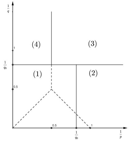
Figure 8: The index sets of Proposition 5

Proof: [Proof of Proposition 4] We divide this proof into two parts.

Sufficiency:

(a)

When $s>\tau_{1}(p,q)$, we can choose $0<\varepsilon\ll 1$ such that $s-\varepsilon>\tau_{1}(p,q)$. Then by Lemma 17 and 29, we have $B_{p,q_{0}}^{s}\hookrightarrow B_{p,q}^{s-\varepsilon}\hookrightarrow W_{p,q}.$

(b)

When $q_{0}\leqslant p\wedge q$, with $q_{0}\geqslant 2$, we know that $\tau_{1}(p,q)=0=\tau_{1}(p,q_{0})$. Then by Lemma 29 and 15, we have $B_{p,q_{0}}\hookrightarrow W_{p,q_{0}}\hookrightarrow W_{p,q}$, when $q\geqslant q_{0}.$

Necessity:

(A)

By Lemma 17, we know that for any $0<\varepsilon\ll 1$, we have $B_{p,q}^{s+\varepsilon}\hookrightarrow B_{p,q_{0}}^{s}$. If we have $B_{p,q_{0}}^{s}\hookrightarrow W_{p,q}$, then we have $B_{p,q}^{s+\varepsilon}\hookrightarrow W_{p,q}$. Then by Lemma 29, we have $s+\varepsilon\geqslant\tau_{1}(p,q)$. Let $\varepsilon\rightarrow 0$, we have $s\geqslant\tau_{1}(p,q).$

(B)

By (1) in Proposition 2, if we know $B_{p,q_{0}}^{s}\hookrightarrow W_{p,q}$, then we have $\ell_{q_{0}}^{s,1}\hookrightarrow\ell_{p}^{0,1}$, $\ell_{q_{0}}^{s+d(1-1/p),1}\hookrightarrow\ell_{p}^{d/p,1}$ and $\ell_{q_{0}}^{s,1}\hookrightarrow\ell_{q}^{0,1}$. Therefore, when $p<q_{0}$, we have $s>0\vee\left(d(1/p+1/q-1)\right)$. When $q<q_{0}$, we have $s>0$.

(C)

When $q_{0}\geqslant p\geqslant 2>q$, if we have $B_{p,q_{0}}^{s}\hookrightarrow W_{p,q}$, then by Lemma 17, we have $L^{s,p}\hookrightarrow F_{p,2}^{s}\hookrightarrow B_{p,q_{0}}^{s}\hookrightarrow W_{p,q}$. By Theorem 1, we have $s>\tau_{1}(p,q)=d(1/q-1/2).$

In conclusion, the necessity of (1) follows by (A), the necessity of (2) following by (B), the necessity of (3) follows by (B), (C).

Proof: [Proof of Proposition 5] By the same argument as in (a) and (A) of the proof of Proposition 4, we only need to prove the sufficiency of Condition (1) and the necessity of Condition (2), (3).

Sufficiency of (1):

(a)

When $p=q,q_{0}\leqslant p$, we know that $W_{p,p}=M_{p,p},s\geqslant\tau_{1}(p,p)=\tau(p,p)$. Then by Lemma 29 and 17, we have $B_{p,q_{0}}^{s}\hookrightarrow B_{p,p}^{s}\hookrightarrow M_{p,p}=W_{p,p}$.

(b)

When $q=q_{0},p\geqslant q_{0},s\geqslant\tau_{1}(p,q_{0})$, by Lemma 28, we have $B_{p,q_{0}}^{s}\hookrightarrow W_{p,q_{0}}$.

(c)

When $p=q_{0}\leqslant q$, by Lemma 17, we have $B_{q_{0},q_{0}}^{s}\hookrightarrow F_{q_{0},2}^{s}=h_{q_{0}}^{s}$. Then by Theorem 3, we have $h_{q_{0}}^{s}\hookrightarrow W_{q_{0},q}$ when $s\geqslant\tau_{1}(q_{0},q)$.

The sufficiency follows by the interpolation of (a), (b), (c).

Necessity of (2): by the same argument as in (B) of the proof of Proposition 4, when $p<q_{0}$, we have $s>0\vee\left(d\left(1/p+1/q-1\right)\right).$

Necessity of (3): by (2) in Proposition 2, we have $\ell_{q_{0}}^{s+d(1-1/p),1}\hookrightarrow\ell_{q}^{d/q,1}$. So, when $q<q_{0}$, we have $s>d(1/p+1/q+1)=\tau_{1}(p,q).$

Remark 5.

As for the case of $q<q_{0}\wedge 2$ and $p>q_{0}\vee 2$ (see $(1/p,1/q)\in(4)$ in Figure 7 and 8), by the argument above, we know that the embedding $B_{p,q_{0}}^{s}\hookrightarrow W_{p,q}$ holds when $s>\tau_{1}(p,q)=d(1/q-1/2)$. But we can not get the necessity of this condition. The reason, in some sense, is the lack of the randomization of Besov spaces in contrast with Sobolev spaces. This is a remaining question.

Remark 6.

The proof of Theorem 8 is similar to the proof above. We omit it as well.

7 Proof of Theorem 9 and 10

We only give the proof of Theorem 9. The proof of Theorem 10 is similar. We first consider the special case of $s=0$ in Theorem 9. We have

Proposition 6.

Let $0<p,q,u,v\leqslant\infty$, then $M_{p,u}\hookrightarrow W_{p,q}\hookrightarrow M_{p,v}$ if and only if $u\leqslant p\wedge q,v\geqslant p\vee q$.

Proof: We divide this proof into two parts.

Sufficiency: by the embedding relationship of $M_{p,q}$ and $W_{p,q}$ (Lemma 15), we have

$$M_{p,u}\hookrightarrow M_{p,p\wedge q}\hookrightarrow W_{p,p\wedge q}\hookrightarrow W_{p,q}\mathchar 24635\relax\;$$

$$W_{p,q}\hookrightarrow W_{p,p\vee q}\hookrightarrow M_{p,p\vee q}\hookrightarrow M_{p,v}.$$

Necessity: we only prove the part of $M_{p,u}\hookrightarrow W_{p,q}$, one can prove the part of $W_{p,q}\hookrightarrow M_{p,v}$ in the same way.

If we have $M_{p,u}\hookrightarrow W_{p,q}$, which means that

$$\left\|f\right\|_{W_{p,q}}\lesssim\left\|f\right\|_{M_{p,u}}.$$ (5)

(i)

Choose $\eta\in\mathscr{S}$ such that $\Box_{0}\eta=\eta$, then take $f=\sum_{k\in{\mathbb{Z}}^{d}}a_{k}e^{ikx}\eta(x)$, then we know that $\Box_{k}f=a_{k}e^{ikx}\eta(x)$. Therefore, we have

$$\left\|f\right\|_{M_{p,u}}\approx\left\|a_{k}\right\|_{\ell_{k}^{u}},\quad\left\|f\right\|_{W_{p,q}}\approx\left\|a_{k}\right\|_{\ell_{k}^{q}}.$$

Take it into (5), we have $u\leqslant q$.

(ii)

Take $f^{N}=\sum_{k\in{\mathbb{Z}}^{d}}a_{k}T_{Nk}(e^{ikx}\eta(x))$, where $T_{Nk}f(x)=f(x-Nk)$. Then we have $\Box_{k}f^{N}=a_{k}T_{Nk}(e^{ikx}\eta(x))$. So, we know that

$$\left\|f^{N}\right\|_{M_{p,u}} \approx\left\|a_{k}\right\|_{\ell_{k}^{u}},$$

$$\lim_{N\rightarrow\infty}\left\|f^{N}\right\|_{W_{p,q}} =\lim_{N\rightarrow\infty}\left\|\left\|a_{k}T_{Nk}(e^{ikx}\eta(x))\right\|_{\ell_{k}^{q}}\right\|_{p}$$

$$=\lim_{N\rightarrow\infty}\left\|\left\|a_{k}T_{Nk}(e^{ikx}\eta(x))\right\|_{\ell_{k}^{p}}\right\|_{p}\approx\left\|a_{k}\right\|_{\ell_{k}^{p}},$$

where we use the almost orthogonality of $\left\{T_{Nk}f\right\}_{k\in{\mathbb{Z}}^{d}}$ to take the limitation above. Take the estimates into (5), we have $u\leqslant p$.

Then, we could give the proof of Theorem 9.

Proof: [Proof of Theorem 9] We divide this proof into two parts.

Sufficiency: by the embedding of $M_{p,q}^{s}$, we have $M_{p_{1},q_{1}}^{s}\hookrightarrow M_{p,p\wedge q}$, then by Proposition 6, we have $M_{p,p\wedge q}\hookrightarrow W_{p,q}$.

Necessity:

(i)

Take $f$ as in (i) of the proof of Proposition 6, we can get $\ell_{q_{1}}^{s,0}\hookrightarrow\ell_{q}^{0,0}$.

(ii)

Take $f$ as in (ii) of the proof of Proposition 6, we can get $\ell_{q_{1}}^{s,0}\hookrightarrow\ell_{q}^{0,0}$.

(iii)

By Proposition 1, we have $p_{1}\leqslant p.$

Combine (i) and (ii), we have $\ell_{q_{1}}^{s,0}\hookrightarrow\ell_{p\wedge q}^{s,0}$. Then by Lemma 20, we have the conditions as desired.

8 Proof of Theorem 11 and 12

8.1 Proof of Theorem 11

We first give some propositions, which play a great role in our proofs.

Proposition 7.

Let $\alpha\in(0,1)$. We have $M_{\infty,2}^{0,\alpha}\hookrightarrow W_{\infty,2}$.

Proof: By the $\alpha$-BAPU in Definition 2, we have $\widehat{f}=\sum_{k\in{\mathbb{Z}}^{d}}\eta_{k}^{\alpha}\widehat{f}.$ By the property of STFT, we know $\lvert V_{g}f(x,\xi)\rvert=\lvert V_{\widehat{g}}\widehat{f}(\xi,-x)\rvert$, so we have

$$\left\|f\right\|_{W_{\infty,2}} =\left\|\|V_{g}\widehat{f}(\xi,x)\|_{L_{\xi}^{2}}\right\|_{L_{x}^{\infty}}$$

$$=\left\|\|\sum_{k\in{\mathbb{Z}}^{d}}V_{g}(\eta_{k}^{\alpha}\widehat{f})(\xi,x)\|_{L_{\xi}^{2}}\right\|_{L_{x}^{\infty}}.$$ (6)

If we choose window function $g$ with ${\mbox{supp}\ }g\subseteq[0,1]^{d}$, then ${\mbox{supp}\ }V_{g}(\eta_{k}^{\alpha}\widehat{f})(\cdot,x)\subseteq{\mbox{supp}\ }\eta_{k}^{\alpha}+[0,1]^{d}\subseteq 2\ {\mbox{supp}\ }\eta_{k}^{\alpha}$ for any $x\in{\mathbb{R}}^{d}$. By the definition of $\eta_{k}^{\alpha}$, we know $\left\{2\ {\mbox{supp}\ }\eta_{k}^{\alpha}\right\}_{k\in{\mathbb{Z}}^{d}}$ are bounded overlapped. Then by the orthogonality of $L_{\xi}^{2}$, we have

$$\eqref{eq-w-infty-2} \lesssim\left\|\|\|V_{g}(\eta_{k}^{\alpha}\widehat{f})(\xi,x)\|_{L_{\xi}^{2}}\|_{\ell_{k}^{2}}\right\|_{L_{x}^{\infty}}$$

$$\left\|\|\|V_{g}(\eta_{k}^{\alpha}\widehat{f})(\xi,x)\|_{L_{\xi}^{2}}\|_{L_{x}^{\infty}}\right\|_{\ell_{k}^{2}}=\left\|\|\Box_{k}^{\alpha}f\|_{W_{\infty,2}}\right\|_{\ell_{k}^{2}},$$

where we use the Minkowski’s inequality at the last inequality. By Theorem 1, we have $L^{\infty}\hookrightarrow W_{\infty,2}$, which means that $\left\|u\right\|_{W_{\infty,2}}\lesssim\left\|u\right\|_{\infty}$. Take this into the inequality above, we have

$$\eqref{eq-w-infty-2}\lesssim\left\|\|\Box_{k}^{\alpha}f\|_{\infty}\right\|_{\ell_{k}^{2}}=\left\|f\right\|_{M_{\infty,2}^{0,\alpha}}.$$

Combine the estimates above, we have $\left\|f\right\|_{W_{\infty,2}}\lesssim\left\|f\right\|_{M_{\infty,2}^{0,\alpha}}$ which means that $M_{\infty,2}^{0,\alpha}\hookrightarrow W_{\infty,2}$.

Proposition 8.

Let $\alpha\in(0,1)$, $0<q\leqslant 1,s=\alpha d(1/q-1/2)$. Then we have $M_{\infty,q}^{s,\alpha}\hookrightarrow W_{\infty,q}.$

Proof: For $f=\sum_{k\in{\mathbb{Z}}^{d}}\Box_{k}^{\alpha}f$, we have

$$\left\|f\right\|_{W_{\infty,q}} =\left\|\|V_{g}f(x,\xi)\|_{L_{\xi}^{q}}\right\|_{L_{x}^{\infty}}$$

$$=\left\|\|\sum_{k\in{\mathbb{Z}}^{d}}V_{g}\left(\Box_{k}^{\alpha}f\right)(x,\xi)\|\right\|_{L_{x}^{\infty}}.$$ (7)

Then by quasi-triangular inequality of $L_{\xi}^{q}$ and Minkowski’s inequality, we have

$$\eqref{eq-w-infty-1} \leqslant\left\|\|\|V_{g}\left(\Box_{k}^{\alpha}f\right)(x,\xi)\|_{L_{\xi}^{q}}\|_{\ell_{k}^{q}}\right\|_{L_{x}^{\infty}}$$

$$\leqslant\left\|\|\|V_{g}\left(\Box_{k}^{\alpha}f\right)(x,\xi)\|_{L_{\xi}^{q}}\|_{L_{x}^{\infty}}\right\|_{\ell_{k}^{q}}$$

$$=\left\|\|\Box_{k}^{\alpha}f\|_{W_{\infty,q}}\right\|_{\ell_{k}^{q}}.$$ (8)

For any $k\in{\mathbb{Z}}^{d}$, denote $\wedge_{k}=\left\{\ell\in{\mathbb{Z}}^{d}:\Box_{\ell}\Box_{k}^{\alpha}\neq 0\right\}$. Obviously, we know that $\#\wedge_{k}\approx\left\langle k\right\rangle^{\alpha d/(1-\alpha)}$. Then by Hölder’s inequality, we have

$$\left\|\Box_{k}^{\alpha}f\right\|_{W_{\infty,q}} =\left\|\|\Box_{\ell}\Box_{k}^{\alpha}f\|_{\ell_{\ell\in\wedge_{k}}^{q}}\right\|_{\infty}$$

$$\leqslant\left\|\|\Box_{\ell}\Box_{k}^{\alpha}f\|_{\ell_{\ell\in\wedge_{k}}^{2}}\left(\#\wedge_{k}\right)^{1/q-1/2}\right\|_{\infty}$$

$$=\left\langle k\right\rangle^{\frac{\alpha d}{1-\alpha}(1/q-1/2)}\left\|\Box_{k}^{\alpha}f\right\|_{W_{\infty,2}}.$$

By Theorem 1, we have $L^{\infty}\hookrightarrow W_{\infty,2}$. Use this embedding and take the estimate above into (8.1), we have

$$\left\|f\right\|_{W_{\infty,q}}\lesssim\left\|\left\langle k\right\rangle^{\frac{\alpha d}{1-\alpha}(1/q-1/2)}\|\Box_{k}^{\alpha}f\|_{\infty}\right\|_{\ell_{k}^{q}}=\left\|f\right\|_{M_{\infty,q}^{s,\alpha}},$$

which means that $M_{\infty,q}^{s,\alpha}\hookrightarrow W_{\infty,q}.$

Proposition 9.

Let $\alpha\in(0,1),0<p\leqslant 1,s>\alpha d(1/p-1)+d(1-\alpha)/p$. Then we have $M_{p,\infty}^{s,\alpha}\hookrightarrow W_{p,\infty}.$

Proof: By the quasi triangular inequality as in the proof of Proposition 8, we have

$$\left\|f\right\|_{W_{p,\infty}}\lesssim\left\|\|\Box_{k}^{\alpha}f\|_{W_{p,\infty}}\right\|_{\ell_{k}^{p}}.$$ (9)

By STFT, we have

$$\left\|\Box_{k}^{\alpha}f\right\|_{W_{p,\infty}} =\left\|\|V_{g}\left(\eta_{k}^{\alpha}\widehat{f}\right)(\xi,x)\|_{L_{\xi}^{\infty}}\right\|_{L_{x}^{p}}$$

$$=\left\|\|{\mathscr{F}^{-1}}\left(\eta_{k}^{\alpha}\widehat{f}T_{\xi}g\right)(x)\|L_{\xi}^{\infty}\right\|_{L_{x}^{p}}$$

$$=\left\|\|\Box_{k}^{\alpha}f*{\mathscr{F}^{-1}}\left(T_{\xi}g\widetilde{\eta_{k}^{\alpha}}\right)(x)\|_{L_{\xi}^{\infty}}\right\|_{L_{x}^{p}}$$

$$\leqslant\left\|\lvert\Box_{k}^{\alpha}f\rvert*\left\|{\mathscr{F}^{-1}}\left(T_{\xi}g\widetilde{\eta_{k}^{\alpha}}\right)\right\|_{L_{\xi}^{\infty}}(x)\right\|_{L_{x}^{p}},$$ (10)

where $T_{\xi}f(x)=f(x-\xi)$ is the translation operator and $\eta_{k}^{\alpha}\widetilde{\eta_{k}^{\alpha}}=\eta_{k}^{\alpha}.$ By the properties of Fourier transform ${\mathscr{F}}$, we have

$$\left\|{\mathscr{F}^{-1}}\left(T_{\xi}g\widetilde{\eta_{k}^{\alpha}}\right)\right\|_{L_{\xi}^{\infty}} =\left\|M_{\xi}\widehat{g}*{\mathscr{F}^{-1}}\widetilde{\eta_{k}^{\alpha}}\right\|_{L_{\xi}^{\infty}}$$

$$\leqslant\left\|M_{\xi}\widehat{g}\right\|_{L_{\xi}^{\infty}}*\lvert{\mathscr{F}^{-1}}\eta_{k}^{\alpha}\rvert$$

$$=\widehat{g}*\lvert{\mathscr{F}^{-1}}\eta_{k}^{\alpha}\rvert,$$

where $M_{\xi}f(x)=e^{i\xi x}f(x)$ is the modulation operator, and we can assume $\widehat{g}\geqslant 0$. Take this into (8.1), we have

$$\left\|\Box_{k}^{\alpha}f\right\|_{W_{p,\infty}}\lesssim\left\|\lvert\Box_{k}^{\alpha}f\rvert*\widehat{g}*\lvert{\mathscr{F}^{-1}}\eta_{k}^{\alpha}\rvert\right\|_{p}.$$

Then by Lemma 23, we have

$$\left\|\Box_{k}^{\alpha}f\right\|_{W_{p,\infty}}\lesssim\left\langle k\right\rangle^{\frac{\alpha d}{1-\alpha}(1/p-1)}\left\|\Box_{k}^{\alpha}f\right\|_{p}.$$

Take this into (9), we have

$$\left\|f\right\|_{W_{p,\infty}}\lesssim\left\|\left\langle k\right\rangle^{\frac{\alpha d}{1-\alpha}(1/p-1)}\left\|\Box_{k}^{\alpha}f\right\|_{p}\right\|_{\ell_{k}^{p}}=\left\|f\right\|_{M_{p,p}^{\alpha d(1/p-1),\alpha}}.$$

When $s>\alpha d(1/p-1)+d(1-\alpha)/p$, by Lemma 18, we have $M_{p,\infty}^{s,\alpha}\hookrightarrow M_{p,p}^{\alpha d(1/p-1),\alpha}$, take this embedding into the estimate above, we have

$$\left\|f\right\|_{W_{p,\infty}}\lesssim\left\|f\right\|_{M_{p,p}^{\alpha d(1/p-1),\alpha}}\lesssim\left\|f\right\|_{M_{p,\infty}^{s,\alpha}},$$

which means that $M_{p,\infty}^{s,\alpha}\hookrightarrow W_{p,\infty}.$

Proposition 10.

Let $0<p,q\leqslant\infty,s\in{\mathbb{R}},\alpha\in(0,1)$. Then

(1)

$M_{p,q}^{s,\alpha}\hookrightarrow W_{p,q}\Longrightarrow\ell_{q}^{s/(1-\alpha),0}\hookrightarrow\ell_{p}^{0,0}\mathchar 24635\relax\;$

(2)

$W_{p,q}\hookrightarrow M_{p,q}^{s,\alpha}\Longrightarrow\ell_{p}^{0,0}\hookrightarrow\ell_{q}^{s/(1-\alpha),0}.$

Proof: We only prove the first assertion. The second assertion can be prove in a similar way.

If we know $M_{p,q}^{s,\alpha}\hookrightarrow W_{p,q}$, then we

$$\left\|f\right\|_{W_{p,q}}\lesssim\left\|f\right\|_{M_{p,q}^{s,\alpha}}.$$ (11)

For any $k\in{\mathbb{Z}}^{d}$, denote $\xi_{k}=\left\langle k\right\rangle^{\alpha/(1-\alpha)}k$. For any $N\geqslant 1,N\in{\mathbb{N}}$, take $f^{N}=\sum_{k\in{\mathbb{Z}}^{d}}a_{k}T_{Nk}{\mathscr{F}^{-1}}\sigma(\xi-\xi_{k})$, where $\sigma\in\mathscr{S}$ with ${\mbox{supp}\ }\sigma\subseteq[-1/4,1/4]^{d}$. Then we know that $\Box_{k}^{\alpha}f^{N}=a_{k}T_{Nk}\left({\mathscr{F}^{-1}}\sigma(\xi-\xi_{k})\right),$ $\Box_{\ell}f^{N}=a_{\ell}T_{N\ell}\left({\mathscr{F}^{-1}}\sigma(\xi-\xi_{\ell})\right)$. So, we have

$$\left\|f^{N}\right\|_{M_{p,q}^{s,\alpha}} =\left\|a_{k}\left\langle k\right\rangle^{s/(1-\alpha)}\|T_{Nk}\left({\mathscr{F}^{-1}}\sigma(\xi-\xi_{k})\right)\|\right\|_{\ell_{k}^{q}}$$

$$=\left\|a_{k}\left\langle k\right\rangle^{s/(1-\alpha)}\right\|_{\ell_{k}^{q}}=\left\|a_{k}\right\|_{\ell_{q}^{s/(1-\alpha),0}}.$$

$$\left\|f^{N}\right\|_{W_{p,q}} =\left\|\|\Box_{k}f^{N}\|_{\ell_{k}^{q}}\right\|_{p}$$

$$=\left\|\|a_{k}T_{Nk}\left({\mathscr{F}^{-1}}\sigma(\xi-\xi_{k})\right)\|_{\ell_{k}^{q}}\right\|_{p}=\left\|\|a_{k}T_{Nk}\left({\mathscr{F}^{-1}}\sigma\right)\|_{\ell_{k}^{q}}\right\|_{p}.$$

Take $N\rightarrow\infty$, use the almost orthogonality of $\left\{T_{Nk}\left({\mathscr{F}^{-1}}\sigma\right)\right\}_{k\in{\mathbb{Z}}^{d}}$, we have

$$\lim_{N\rightarrow\infty}\left\|f^{N}\right\|_{W_{p,q}}=\left\|\|a_{k}{\mathscr{F}^{-1}}\sigma\|_{\ell_{k}^{q}}\right\|_{p}=\left\|a_{k}\right\|_{\ell_{p}^{0,0}}.$$

Take the estimates of $f^{N}$ into (11), we have

$$\left\|a_{k}\right\|_{\ell_{p}^{0,0}}\lesssim\left\|a_{k}\right\|_{\ell_{q}^{s/(1-\alpha),0}},$$

which means that $\ell_{q}^{s/(1-\alpha),0}\hookrightarrow\ell_{p}^{0,0}.$

Proposition 11.

Let $0<q\leqslant\infty,0<p<\infty,s\in{\mathbb{R}},\alpha\in(0,1)$. Then

(1)

$M_{p,q}^{s,\alpha}\hookrightarrow W_{p,q}\Longrightarrow s\geqslant\alpha d(1/q-1/2)\mathchar 24635\relax\;$

(2)

$W_{p,q}\hookrightarrow M_{p,q}^{s,\alpha}\Longrightarrow s\leqslant\alpha d(1/q-1/2).$

Proof: We only give the proof of the assertion (1). For any $k\in{\mathbb{Z}}^{d}$, denote $\wedge_{k}=\left\{\ell\in{\mathbb{Z}}^{d}:\Box_{\ell}\Box_{k}^{\alpha}=\Box_{\ell}\right\}$. One can easily see that $\#\wedge_{k}\approx\left\langle k\right\rangle^{\alpha d/(1-\alpha)}.$ Let $\overrightarrow{\omega}=\left\{\omega_{k}\right\}_{k\in{\mathbb{Z}}^{d}}$ be a sequence of independent random variables (for instance, one can choose the Rademacher functions). Denote $f^{\overrightarrow{\omega}}=\sum_{\ell\in\wedge_{k}}\omega_{k}{\mathscr{F}^{-1}}(\sigma(\xi-\ell))$. Then by orthogonality, we have

$$\left\|f^{\overrightarrow{\omega}}\right\|_{W_{p,q}} =\left\|\|\omega_{\ell}{\mathscr{F}^{-1}}(\sigma(\xi-\ell)\|_{\ell_{\ell\in\wedge_{k}}^{q}}\right\|_{p}$$

$$=\left(\#\wedge_{k}\right)^{1/q}=\left\langle k\right\rangle^{\frac{\alpha d}{q(1-\alpha)}}\mathchar 24635\relax\;$$

$$\left\|f^{\overrightarrow{\omega}}\right\|_{M_{p,q}^{s,\alpha}} =\left\langle k\right\rangle^{s/(1-\alpha)}\left\|f^{\overrightarrow{\omega}}\right\|_{p}.$$

Note that $0<p<\infty$, then by Khinchin’s inequality, we have

$$\left(\mathbb{E}\left\|f^{\overrightarrow{\omega}}\right\|_{p}^{p}\right)^{1/p} \approx\left\|\left(\sum_{\ell\in\wedge_{k}}\lvert{\mathscr{F}^{-1}}\left(\sigma(\xi-\ell)\right)\rvert^{2}\right)^{1/2}\right\|_{p}$$

$$\approx\left(\#\wedge_{k}\right)^{1/2}=\left\langle k\right\rangle^{\frac{\alpha d}{2(1-\alpha)}}.$$

Take these estimates of $f^{\overrightarrow{\omega}}$ into (11), we have

$$\left\langle k\right\rangle^{\frac{\alpha d}{q(1-\alpha)}}\lesssim\left\langle k\right\rangle^{\frac{s}{1-\alpha}+\frac{\alpha d}{2(1-\alpha)}}.$$

Take $\left\langle k\right\rangle\rightarrow\infty$, we have $s\geqslant\alpha d(1/q-1/2).$

Proposition 12.

Let $0<p,q\leqslant\infty,s\in{\mathbb{R}},\alpha\in(0,1)$. Then

(1)

$M_{p,q}^{s,\alpha}\hookrightarrow W_{p,q}\Longrightarrow\ell_{q}^{(s+\alpha d(1-1/p))/(1-\alpha),0}\hookrightarrow\ell_{p}^{\alpha d/((1-\alpha)q),0}\mathchar 24635\relax\;$

(2)

$W_{p,q}\hookrightarrow M_{p,q}^{s,\alpha}\Longrightarrow\ell_{p}^{\alpha d/((1-\alpha)q),0}\hookrightarrow\ell_{q}^{(s+\alpha d(1-1/p))/(1-\alpha),0}.$

Proof: We only give the proof of assertion (1). For any $k\in{\mathbb{Z}}^{d}$, denote $\wedge_{k}=\left\{\ell\in{\mathbb{Z}}^{d}:\Box_{\ell}\Box_{k}^{\alpha}=\Box_{\ell}\right\}$. For any $N\geqslant 1,N\in{\mathbb{N}}$, denote $f^{N}=\sum_{k\in{\mathbb{Z}}^{d}}a_{k}T_{Nk}\left({\mathscr{F}^{-1}}\eta_{k}^{\alpha}\right).$ Then by orthogonality, we have

$$\left\|f^{N}\right\|_{M_{p,q}^{s,\alpha}} =\left\|\|T_{Nk}\left({\mathscr{F}^{-1}}\eta_{k}^{\alpha}\right)\|_{p}a_{k}\left\langle k\right\rangle^{s/(1-\alpha)}\right\|_{\ell_{k}^{q}}$$

$$=\left\|a_{k}\left\langle k\right\rangle^{\frac{\alpha d}{1-\alpha}(1-\frac{1}{p})+\frac{s}{1-\alpha}}\right\|=\left\|a_{k}\right\|_{\ell_{q}^{\frac{s+\alpha d(1-1/p)}{1-\alpha},0}}\mathchar 24635\relax\;$$

$$\left\|f^{N}\right\|_{W_{p,q}} =\left\|\|\Box_{\ell}f^{N}\|_{\ell_{\ell}^{q}}\right\|_{p}\geqslant\left\|\|\|\Box_{\ell}f^{N}\|_{\ell_{\ell\in\wedge_{k}}^{q}}\|_{\ell_{k}^{q}}\right\|_{p}$$

$$=\left\|\|a_{k}T_{Nk}\|{\mathscr{F}^{-1}}\sigma_{\ell}\|_{\ell_{\ell\in\wedge_{k}}^{q}}\|_{\ell_{k}^{q}}\right\|_{p}$$

$$=\left\|\|a_{k}T_{Nk}({\mathscr{F}^{-1}}\sigma)\left(\#\wedge_{k}\right)^{1/q}\|_{\ell_{k}^{q}}\right\|_{p}.$$

Let $N\rightarrow\infty,$ use the almost orthogonality of $\left\{T_{Nk}({\mathscr{F}^{-1}}\sigma)\right\}_{k\in{\mathbb{Z}}^{d}}$, we have

$$\lim_{N\rightarrow\infty}\left\|f^{N}\right\|_{W_{p,q}}=\left\|a_{k}\left\langle k\right\rangle^{\frac{\alpha d}{q(1-\alpha)}}\right\|_{\ell_{k}^{p}}=\left\|a_{k}\right\|_{\ell_{p}^{\frac{\alpha d}{q(1-\alpha)},0}}$$

Take the estimates of $f^{N}$ into (11), we have

$$\left\|a_{k}\right\|_{\ell_{p}^{\frac{\alpha d}{q(1-\alpha)},0}}\lesssim\left\|a_{k}\right\|_{\ell_{q}^{\frac{s+\alpha d(1-1/p)}{1-\alpha},0}},$$

which means that $\ell_{q}^{\frac{s+\alpha d(1-1/p)}{1-\alpha},0}\hookrightarrow\ell_{p}^{\frac{\alpha d}{q(1-\alpha)},0}.$

Then we can prove Theorem 11.

Proof: [Proof of Theorem 11] We divide the proof into two parts.

Sufficiency:

(a)

When $p=q$, we know $\tau_{1}(p,q)=\tau(p,q)$, $W_{p,q}=M_{p,q}$. When $s\geqslant\alpha\tau(p,q)$, by Lemma 19, we have $M_{p,q}^{s,\alpha}\hookrightarrow M_{p,q}=W_{p,q}$.

(b)

When $p\geqslant q,p\leqslant 2$, we know $\tau_{1}(p,q)=\tau(p,q)=d(1/p+1/q-1).$ When $s\geqslant\alpha\tau_{1}(p,q)$, by Lemma 19 and 15, we have $M_{p,q}^{s,\alpha}\hookrightarrow M_{p,q}\hookrightarrow W_{p,q}$.

(c)

When $p=\infty,q=2,s\geqslant\alpha\tau_{1}(p,q)=0$, by Proposition 7, we have $M_{p,q}^{s,\alpha}\hookrightarrow W_{p,q}$.

(d)

When $p=\infty,0<q\leqslant 1,s\geqslant\alpha\tau_{1}(p,q)=\alpha d(1/q-1/2)$, by Proposition 8, we have $M_{p,q}^{s,\alpha}\hookrightarrow W_{p,q}$.

(e)

When $0<p\leqslant 1,q=\infty$, we know $\tau_{1}(p,q)=d(1/p-1)$. When $s>\alpha d(1/p-1)+d(1-\alpha)/p$, by Proposition 9, we have $M_{p,q}^{s,\alpha}\hookrightarrow W_{p,q}$.

The sufficiency follows by interpolations of (a)-(e).

Necessity:

(A)

By Proposition 10, we have $\ell_{q}^{s/(1-\alpha),0}\hookrightarrow\ell_{p}^{0,0}$. By lemma 20, we have $s\geqslant 0$. Moreover, when $q>p$, we have $s>d(1-\alpha)(1/p-1/q).$

(B)

When $p\geqslant q,0<p\leqslant 2$, we know that $\tau_{1}(p,q)=\tau(p,q)$. If we have $M_{p,q}^{s,\alpha}\hookrightarrow W_{p,q}$, then by Lemma 19, we have $B_{p,q}^{s+(1-\alpha)\tau(p,q)}\hookrightarrow M_{p,q}^{s,\alpha}\hookrightarrow W_{p,q}$. By Theorem 5, we have $s+(1-\alpha)\tau(p,q)\geqslant\tau_{1}(p,q)$. So, we have $s\geqslant\alpha\tau_{1}(p,q).$

C

When $0\leqslant p<\infty,0<q\leqslant 2$, by Proposition 11, we have $s\geqslant\alpha d(1/q-1/2)$.

(D)

When $p=\infty,0<q\leqslant 2$, if $M_{p,q}^{s,\alpha}\hookrightarrow W_{p,q}$ holds for some $s<\alpha d(1/q-1/2)$. Take interpolation with $M_{2,q}^{\alpha d(1/q-1/2),\alpha}\hookrightarrow W_{2,q}$ given in (b), we have $M_{p,q}^{s,\alpha}\hookrightarrow W_{p,q}$ holds for some $s<\alpha d(1/q-1/2)$, which is contraction with (C).

(E)

By Proposition 12, we have $\ell_{q}^{(s+\alpha d(1-1/p))/(1-\alpha),0}\hookrightarrow\ell_{p}^{\alpha d/((1-\alpha)q),0}$. Then by Lemma 20, we have $s\geqslant\alpha d(1/p+1/q-1)$. Moreover, when $p<q$, we have $s>\alpha d(1/p+1/q-1)+d(1-\alpha)(1/p-1/q).$

Combine (A)-(E), we can get the necessity as desired.

8.2 Proof of Theorem 12

We first give some propositions, which play a great role in our proofs.

Proposition 13.

Let $0<p\leqslant 1,s=-\alpha d/2$. Then we have $W_{p,\infty}\hookrightarrow M_{p,\infty}^{s,\alpha}.$

Proof: By definition of $M_{p,q}^{s,\alpha}$, we have

$$\left\|f\right\|_{M_{p,\infty}^{s,\alpha}}=\sup_{k\in{\mathbb{Z}}^{d}}\left\langle k\right\rangle^{\frac{s}{1-\alpha}}\left\|\Box_{k}^{\alpha}f\right\|_{p}.$$ (12)

By Theorem 4, we have $W_{p,2}\hookrightarrow h_{p}\hookrightarrow L^{p}$. Then we have $\left\|\Box_{k}^{\alpha}f\right\|_{p}\lesssim\left\|\Box_{k}^{\alpha}f\right\|_{W_{p,2}}$. By STFT, we have

$$\left\|\Box_{k}^{\alpha}f\right\|_{W_{p,2}}=\left\|\|V_{g}\left(\eta_{k}^{\alpha}\widehat{f}\right)(\xi,x)\|_{L_{\xi}^{2}}\right\|_{L_{x}^{p}}.$$

If we choose window function $g$ with ${\mbox{supp}\ }g\subseteq[0,1]^{d}$, then ${\mbox{supp}\ }V_{g}(\eta_{k}^{\alpha}\widehat{f})(\cdot,x)\subseteq{\mbox{supp}\ }\eta_{k}^{\alpha}+[0,1]^{d}\subseteq 2\ {\mbox{supp}\ }\eta_{k}^{\alpha}$ for any $x\in{\mathbb{R}}^{d}$. Denote the Lebesgue measure of a measurable set $A\subseteq{\mathbb{R}}^{d}$ by $\lvert A\rvert$ Then by using Hölder’s inequality into the estimate above, we have

$$\left\|\Box_{k}^{\alpha}f\right\|_{W_{p,2}}\lesssim\left\|\|V_{g}\left(\eta_{k}^{\alpha}\widehat{f}\right)(\xi,x)\|_{L_{\xi}^{\infty}}\lvert{\mbox{supp}\ }\eta_{k}^{\alpha}\rvert^{1/2}\right\|_{L_{x}^{p}}=\left\langle k\right\rangle^{\frac{\alpha d}{2(1-\alpha)}}\left\|\Box_{k}^{\alpha}f\right\|_{W_{p,\infty}}.$$

Take this estimate into (12), we have

$$\left\|f\right\|_{M_{p,\infty}^{s,\alpha}}\lesssim\sup_{k\in{\mathbb{Z}}^{d}}\left\|\Box_{k}^{\alpha}f\right\|_{W_{p,\infty}}.$$ (13)

Then by Lemma 24, we have

$$\left\|\Box_{k}^{\alpha}f\right\|_{W_{p,\infty}}\lesssim\left\|{\mathscr{F}^{-1}}\eta_{k}^{\alpha}\right\|_{W_{p,\infty}}\left\|f\right\|_{W_{p,\infty}}.$$

By the scaling of $M_{\infty,p}$ with $0<p\leqslant 1$ (Lemma 25), we have

$$\left\|{\mathscr{F}^{-1}}\eta_{k}^{\alpha}\right\|_{W_{p,\infty}}=\left\|\eta_{k}^{\alpha}\right\|_{M_{\infty,p}}\lesssim\left\|\eta(\xi-k)\right\|_{M_{\infty,p}}=\left\|\eta\right\|_{M_{\infty,p}}\lesssim 1.$$

Take the two estimates into (13), we have

$$\left\|f\right\|_{M_{p,\infty}^{s,\alpha}}\lesssim\left\|f\right\|_{W_{p,\infty}},$$

which means that $W_{p,\infty}\hookrightarrow M_{p,\infty}^{s,\alpha}.$

Proposition 14.

Let $0<p\leqslant 1$. Then we have $W_{p,2}\hookrightarrow M_{p,2}^{0,\alpha}.$

Proof: When $0<p\leqslant 1$, by Theorem 4, we have $W_{p,2}\hookrightarrow h_{p}\hookrightarrow L_{p}$. Then by STFT and Minkowski’s inequality, we have

$$\left\|f\right\|_{M_{p,2}^{0,\alpha}} =\left\|\|\Box_{k}^{\alpha}f\|_{p}\right\|_{\ell_{k}^{2}}\lesssim\left\|\|\Box_{k}^{\alpha}f\|_{W_{p,2}}\right\|_{\ell_{k}^{2}}$$

$$=\left\|\|\|V_{g}\Box_{k}^{\alpha}f(x,\xi)\|_{L_{\xi}^{2}}\|_{L_{x}^{p}}\right\|_{\ell_{k}^{2}}$$

$$\leqslant\left\|\|\|V_{g}\Box_{k}^{\alpha}f\|_{L_{\xi}^{2}}\|_{\ell_{k}^{2}}\right\|_{L_{x}^{p}}$$

$$\lesssim\left\|\|V_{g}f(x,\xi)\|_{L_{\xi}^{2}}\right\|_{L_{x}^{p}}=\left\|f\right\|_{W_{p,2}},$$

where we use the orthogonality of $L_{\xi}^{2}$ at the last inequality.

Then, we could give the proof of Theorem 12.

Proof: [Proof of Theorem 12] The necessity of Theorem 12 is similar to the proof of Theorem 11. The sufficiency part follows by interpolations of the following conditions.

(a)

When $p=q,s\leqslant\alpha\tau_{1}(p,q)=\alpha\tau(p,q)$, by Lemma 19, we have $W_{p,q}=M_{p,q}\hookrightarrow M_{p,q}^{s,\alpha}$.

(b)

When $p\leqslant q,p\geqslant 2$, we know $\sigma_{1}(p,q)=\sigma(p,q)$. By Lemma 15 and 19, we have $W_{p,q}\hookrightarrow M_{p,q}\hookrightarrow M_{p,q}^{s,\alpha}.$

(c)

When $0<p\leqslant 1,q=\infty,s\leqslant\alpha\sigma_{1}(p,q)=-\alpha d/2$, by Proposition 13, we have $W_{p,q}\hookrightarrow M_{p,q}^{s,\alpha}.$

(d)

When $0<p\leqslant 1,q=2,s\leqslant\alpha\sigma_{1}(p,q)=0$, by Proposition 14, we have $W_{p,q}\hookrightarrow M_{p,q}^{s,\alpha}.$

(e)

When $p=\infty,0<q\leqslant 1,s<\alpha\sigma_{1}(p,q)+d(1-\alpha)(1/p-1/q)=-d(1-\alpha)/q$. In this case, we know that $\tau(p,q)=d/q.$ By Theorem 6 and Lemma 19, for $0<\varepsilon\ll 1$, we have $W_{p,q}\hookrightarrow B_{p,q}^{-\varepsilon}\hookrightarrow M_{p,q}^{s,\alpha}$.

9 Proof of Theorem 13 and 14

First, we recall some results already known before.

Lemma 30 (Proposition 3.4 in Guo2017Characterization ).

Let $0<p,q,q_{0}\leqslant\infty,0<p_{0}<\infty,s\in{\mathbb{R}}$. Then

(1)

$W_{p,q}\hookrightarrow F_{p_{0},q_{0}}^{s}$ if and only if $p\leqslant p_{0}$ and the following statement holds:

$$\left\|f\right\|_{F_{p_{0},q_{0}}^{s}}\lesssim\left\|f\right\|_{W_{p,q}},\mbox{ for any $f\in\mathscr{S}^{\prime}$ with support in $B(0,1)$.}$$

(2)

$F_{p_{0},q_{0}}^{s}\hookrightarrow W_{p,q}$ if and only if $p_{0}\leqslant p$ and the following statement holds:

$$\left\|f\right\|_{W_{p,q}}\lesssim\left\|f\right\|_{F_{p_{0},q_{0}}^{s}}\mbox{ for any $f\in\mathscr{S}^{\prime}$ with support in $B(0,1)$.}$$

Lemma 31 (Theorem 1.2 in Guo2017Inclusion ).

Let $0<p\leqslant 1,0<q,r\leqslant\infty,s\in{\mathbb{R}}$. Then $F_{p,r}^{s}\hookrightarrow M_{p,q}$ is true if and only if one of the following conditions is satisfied.

(1)

$p\leqslant q,s\geqslant d(1/p+1/q-1)\mathchar 24635\relax\;$

(2)

$p>q,s>d(1/p+1/q-1).$

Lemma 32 (Theorem 1.1 in Guo2017Inclusion ).

Let $0<p\leqslant 1,0<q,r\leqslant\infty,s\in{\mathbb{R}}$. Then $M_{p,q}\hookrightarrow F_{p,r}^{s}$ is true if and only one of the following conditions is satisfied.

(1)

$p\geqslant q,r\geqslant q,s\leqslant 0\mathchar 24635\relax\;$

(2)

$p\geqslant q,r<q,s<0\mathchar 24635\relax\;$

(3)

$p<q,s<d(1/q-1/p).$

Then, we give some propositions which will be used in our proofs.

Proposition 15.

Let $0<q,r\leqslant\infty,0<p<\infty,s\in{\mathbb{R}}$. Then

(1)

When $p\leqslant q$, $F_{p,r}^{s}\hookrightarrow W_{p,q}$ if and only if $F_{p,r}^{s}\hookrightarrow M_{p,q}$;

(2)

When $p\geqslant q$, $W_{p,q}\hookrightarrow F_{p,r}^{s}$ if and only if $M_{p,q}\hookrightarrow F_{p,r}^{s}$.

Proof: Because of the symmetry, we only give the proof of (1).

When $p\leqslant q$, if we have $F_{p,r}^{s}\hookrightarrow W_{p,q}$, then by Lemma 15, we know $F_{p,r}^{s}\hookrightarrow W_{p,q}\hookrightarrow M_{p,q}$.

On the other hand, if we have $F_{p,r}^{s}\hookrightarrow M_{p,q}$, then for any $f\in\mathscr{S}^{\prime}$ , we have

$$\left\|f\right\|_{M_{p,q}}\lesssim\left\|f\right\|_{F_{p,r}^{s}}.$$

By Lemma 16, we know that $\left\|f\right\|_{M_{p,q}}\approx\left\|f\right\|_{W_{p,q}}$ for $f\in\mathscr{S}^{\prime}$ with support in $B(0,1)$. Then by Lemma 30, we have $F_{p,r}^{s}\hookrightarrow W_{p,q}$.

Proposition 16.

Let $0<p,p_{1},q,q_{1}\leqslant\infty$. Then $W_{p,q}\hookrightarrow F_{p_{1},q_{1}}^{s}\Longrightarrow\ell_{q}^{0,1}\hookrightarrow\ell_{q_{1}}^{s,1}$.

Proof: For any $j\geqslant 0$, choose $k_{j}\in\wedge_{j}$, choose $g\in\mathscr{S}$ with support in $[-1/8,1/8]^{d}$, take $f(x)=\sum_{j\geqslant 0}a_{j}{\mathscr{F}^{-1}}g(\cdot-k_{j})(x)=\sum_{j\geqslant 0}a_{j}e^{ik_{j}x}\check{g}(x)$. Then we have

$$\triangle_{j}f=a_{j}{\mathscr{F}^{-1}}g(\cdot-k_{j})\mathchar 24635\relax\;\quad\Box_{k}f=\begin{cases*}a_{j}{\mathscr{F}^{-1}}g(\cdot-k_{j}),&$k=k_{j}\mathchar 24635\relax\;$\\ 0,&else.\end{cases*}$$

So, we know that

$$\left\|f\right\|_{F_{p_{1},q_{1}}^{s}}\approx\left\|a_{j}\right\|_{\ell_{q_{1}}^{s,1}},\quad\left\|f\right\|_{W_{p,q}}\approx\left\|a_{j}\right\|_{\ell_{q}^{0,1}}.$$

Therefore, we have $W_{p,q}\hookrightarrow F_{p_{1},q_{1}}^{s}\Longrightarrow\ell_{q}^{0,1}\hookrightarrow\ell_{q_{1}}^{s,1}$.

Proof: [Proof of Theorem 13] We divide this proof into two parts.

Sufficiency: in case of Condition (1), by Proposition 15, we only need to prove that $F_{p,r}^{s}\hookrightarrow M_{p,q}$, which is true by Lemma 31. In case of Condition (2), by Lemma 31, we know that $F_{p,r}^{s}\hookrightarrow M_{p,q}$. By Lemma 15, we know that $M_{p,q}\hookrightarrow W_{p,q}$, when $p>q$. So, we have $F_{p,r}^{s}\hookrightarrow W_{p,q}.$

Necessity: if we have $F_{p,r}^{s}\hookrightarrow W_{p,q}$, then by Lemma 17, we know that for any $\varepsilon>0$, $F_{p,2}^{s+\varepsilon}\hookrightarrow F_{p,r}^{s}\hookrightarrow W_{p,q}$. Then by the embedding relation of $h_{p}$ spaces and Wiener amalgam spaces (Theorem 3), we know that $s+\varepsilon\geqslant d(1/p+1/q-1)$. Take $\varepsilon\rightarrow 0$, we have $s\geqslant d(1/p+1/q-1)$. When $p>q$, we can choose $p_{1},s_{1}\in{\mathbb{R}}$, such that $p>p_{1}>q,s_{1}-d/p_{1}=s-d/p$. Then by Lemma 17, we have $B_{p_{1},p_{1}}^{s_{1}}\hookrightarrow F_{p,r}^{s}\hookrightarrow W_{p,q}$. Then by (2) in Proposition 2, we have $\ell_{p_{1}}^{s_{1}+d(1-1/p_{1}),1}\hookrightarrow\ell_{q}^{d/q,1}$. So, we have $s_{1}>d(1/p_{1}+1/q-1)$, which is equivalent to $s>d(1/p+1/q-1)$.

Proof: [Proof of Theorem 14] Firstly, by Proposition 15, when $p\geqslant q$, $W_{p,q}\hookrightarrow F_{p,r}^{s}$ is equivalent to $M_{p,q}\hookrightarrow F_{p,r}^{s}$. Then by Lemma 32, we can get the sharp conditions in (1) and (2).

For other cases, by the embedding between $W_{p,q}$ and $h_{p}$ (Theorem 3, 4), we can easily get the sufficiency of Condition (4), (5) and the necessity of Condition (3).

Sufficiency of Condition (3): by Condition (1), we know that $W_{p,p}\hookrightarrow F_{p,p}$. Then by Theorem 4, we know that $W_{p,2}\hookrightarrow h_{p}=F_{p,2}$, then take interpolation, we have $W_{p,q}\hookrightarrow F_{p,q}\hookrightarrow F_{p,r}$, when $r\geqslant q$.

Necessity of Condition (4): If we have $W_{p,q}\hookrightarrow F_{p,r}^{s}$, then by Proposition 16, we have $\ell_{q}^{0,1}\hookrightarrow\ell_{r}^{s,1}$. So, when $r<q$, we have $s<0$.

Remark 7.

When $q>2$, by the argument above, we could only get the sufficiency of $s<\sigma_{1}(p,q)=d(1/q-1/2)$ and the necessity of $s\geqslant d(1/q-1/2)$. As for the endpoint $s=d(1/q-1/2)$. I guess that the embedding $W_{p,q}\hookrightarrow F_{p,r}^{s}$ could only holds when $q\leqslant r$.

References

- \bibcommenthead
- (1) Guo, W., Wu, H., Yang, Q., Zhao, G.: Characterization of inclusion relations between Wiener amalgam and some classical spaces. J. Funct. Anal. 273(1), 404–443 (2017). https://doi.org/10.1016/j.jfa.2017.04.004
- (2) Wiener, N.: On the representation of functions by trigonometrical integrals. Mathematische Zeitschrift 24(1), 575–616 (1926). https://doi.org/10.1007/BF01216799. cited By 59
- (3) Wiener, N.: Tauberian theorems. Annals of Mathematics 33(1), 1–100 (1932). Accessed 2022-04-17
- (4) Wiener, N.: The Fourier Integral and Certain of Its Applications. Cambridge Mathematical Library, p. 201. Cambridge University Press, Cambridge, ??? (1988). https://doi.org/10.1017/CBO9780511662492. Reprint of the 1933 edition, With a foreword by Jean-Pierre Kahane. https://doi.org/10.1017/CBO9780511662492
- (5) Holland, F.: Harmonic analysis on amalgams of and . J. London Math. Soc. (2) 10, 295–305 (1975). https://doi.org/10.1112/jlms/s2-10.3.295
- (6) Feichtinger, H.G.: Banach convolution algebras of Wiener type. In: Functions, Series, Operators, Vol. I, II (Budapest, 1980). Colloq. Math. Soc. János Bolyai, vol. 35, pp. 509–524. North-Holland, Amsterdam, ??? (1983)
- (7) Feichtinger, H.G.: Generalized amalgams, with applications to Fourier transform. Canad. J. Math. 42(3), 395–409 (1990). https://doi.org/10.4153/CJM-1990-022-6
- (8) Feichtinger, H.: Modulation spaces on locally compact abelian groups. (2003)
- (9) Wang, B., Huang, C.: Frequency-uniform decomposition method for the generalized BO, KdV and NLS equations. J. Differential Equations 239(1), 213–250 (2007). https://doi.org/10.1016/j.jde.2007.04.009
- (10) Cunanan, J.: Wiener amalgam spaces and nonlinear evolution equations. (2015)
- (11) Miyachi, A.: On some singular Fourier multipliers. J. Fac. Sci. Univ. Tokyo Sect. IA Math. 28(2), 267–315 (1981)
- (12) Guo, W., Zhao, G.: Sharp estimates of unimodular Fourier multipliers on Wiener amalgam spaces. J. Funct. Anal. 278(6), 108405–44 (2020). https://doi.org/10.1016/j.jfa.2019.108405
- (13) Bényi, A., Gröchenig, K., Okoudjou, K.A., Rogers, L.G.: Unimodular Fourier multipliers for modulation spaces. J. Funct. Anal. 246(2), 366–384 (2007). https://doi.org/10.1016/j.jfa.2006.12.019
- (14) Miyachi, A., Nicola, F., Rivetti, S., Tabacco, A., Tomita, N.: Estimates for unimodular Fourier multipliers on modulation spaces. Proc. Amer. Math. Soc. 137(11), 3869–3883 (2009). https://doi.org/10.1090/S0002-9939-09-09968-7
- (15) Tomita, N.: Unimodular Fourier multipliers on modulation spaces for , 125–131 (2010)
- (16) Chen, J., Fan, D., Sun, L.: Asymptotic estimates for unimodular Fourier multipliers on modulation spaces. Discrete Contin. Dyn. Syst. 32(2), 467–485 (2012). https://doi.org/10.3934/dcds.2012.32.467
- (17) Wang, B., Hudzik, H.: The global Cauchy problem for the NLS and NLKG with small rough data. J. Differential Equations 232(1), 36–73 (2007). https://doi.org/10.1016/j.jde.2006.09.004
- (18) Cordero, E., Nicola, F.: Strichartz estimates in Wiener amalgam spaces for the Schrödinger equation. Math. Nachr. 281(1), 25–41 (2008). https://doi.org/10.1002/mana.200610585
- (19) Cordero, E., Nicola, F.: Remarks on Fourier multipliers and applications to the wave equation. J. Math. Anal. Appl. 353(2), 583–591 (2009). https://doi.org/10.1016/j.jmaa.2008.12.027
- (20) Bényi, A., Okoudjou, K.A.: Local well-posedness of nonlinear dispersive equations on modulation spaces. Bull. Lond. Math. Soc. 41(3), 549–558 (2009). https://doi.org/10.1112/blms/bdp027
- (21) Chaichenets, L., Hundertmark, D., Kunstmann, P., Pattakos, N.: On the existence of global solutions of the one-dimensional cubic NLS for initial data in the modulation space . J. Differential Equations 263(8), 4429–4441 (2017). https://doi.org/10.1016/j.jde.2017.04.020
- (22) Chen, M., Wang, B., Wang, S., Wong, M.W.: On dissipative nonlinear evolutional pseudo-differential equations. Appl. Comput. Harmon. Anal. 48(1), 182–217 (2020). https://doi.org/10.1016/j.acha.2018.04.003
- (23) Oh, T., Wang, Y.: Global well-posedness of the one-dimensional cubic nonlinear Schrödinger equation in almost critical spaces. J. Differential Equations 269(1), 612–640 (2020). https://doi.org/10.1016/j.jde.2019.12.017
- (24) Bhimani, D.G., Carles, R.: Norm inflation for nonlinear Schrödinger equations in Fourier-Lebesgue and modulation spaces of negative regularity. J. Fourier Anal. Appl. 26(6), 78–34 (2020). https://doi.org/10.1007/s00041-020-09788-w
- (25) Borup, L., Nielsen, M.: Banach frames for multivariate -modulation spaces. J. Math. Anal. Appl. 321(2), 880–895 (2006). https://doi.org/10.1016/j.jmaa.2005.08.091
- (26) Han, J., Wang, B.: -modulation spaces (I) scaling, embedding and algebraic properties. J. Math. Soc. Japan 66(4), 1315–1373 (2014). https://doi.org/10.2969/jmsj/06641315
- (27) Guo, W., Fan, D., Zhao, G.: Full characterization of the embedding relations between -modulation spaces. Sci. China Math. 61(7), 1243–1272 (2018). https://doi.org/10.1007/s11425-016-9151-1
- (28) Kobayashi, M., Sugimoto, M.: The inclusion relation between Sobolev and modulation spaces. J. Funct. Anal. 260(11), 3189–3208 (2011). https://doi.org/10.1016/j.jfa.2011.02.015
- (29) Cunanan, J., Kobayashi, M., Sugimoto, M.: Inclusion relations between -Sobolev and Wiener amalgam spaces. J. Funct. Anal. 268(1), 239–254 (2015). https://doi.org/10.1016/j.jfa.2014.10.017
- (30) Guo, W., Fan, D., Wu, H., Zhao, G.: Sharpness of complex interpolation on -modulation spaces. J. Fourier Anal. Appl. 22(2), 427–461 (2016). https://doi.org/10.1007/s00041-015-9424-z
- (31) Grafakos, L.: Modern Fourier Analysis, 2nd edn. Graduate Texts in Mathematics, vol. 250, p. 504. Springer, ??? (2009). https://doi.org/10.1007/978-0-387-09434-2
- (32) Goldberg, D.: A local version of real Hardy spaces. Duke Math. J. 46(1), 27–42 (1979)
- (33) Triebel, H.: Theory of Function Spaces. II. Monographs in Mathematics, vol. 84, p. 370. Birkhäuser Verlag, Basel, ??? (1992). https://doi.org/10.1007/978-3-0346-0419-2
- (34) Gröchenig, K.: Foundations of Time-frequency Analysis. Applied and Numerical Harmonic Analysis, p. 359. Birkhäuser Boston, Inc., Boston, MA, ??? (2001). https://doi.org/10.1007/978-1-4612-0003-1
- (35) Wang, B., Huo, Z., Hao, C., Guo, Z.: Harmonic Analysis Method for Nonlinear Evolution Equations. I, p. 283. World Scientific Publishing Co. Pte. Ltd., Hackensack, NJ, ??? (2011). https://doi.org/10.1142/9789814360746. https://doi.org/10.1142/9789814360746
- (36) Ruzhansky, M., Sugimoto, M., Toft, J., Tomita, N.: Changes of variables in modulation and Wiener amalgam spaces. Math. Nachr. 284(16), 2078–2092 (2011). https://doi.org/10.1002/mana.200910199
- (37) Kobayashi, M.: Modulation spaces for . J. Funct. Spaces Appl. 4(3), 329–341 (2006). https://doi.org/10.1155/2006/409840
- (38) Guo, W., Chen, J., Fan, D., Zhao, G.: Characterizations of some properties on weighted modulation and Wiener amalgam spaces. Michigan Math. J. 68(3), 451–482 (2019). https://doi.org/10.1307/mmj/1552442712
- (39) Sugimoto, M., Tomita, N.: The dilation property of modulation spaces and their inclusion relation with Besov spaces. J. Funct. Anal. 248(1), 79–106 (2007). https://doi.org/10.1016/j.jfa.2007.03.015
- (40) Lu, Y.: Sharp embedding between Besov-Triebel-Sobolev spaces and modulation spaces. arXiv e-prints, 2108–12106 (2021) arXiv:2108.12106 [math.FA]
- (41) Guo, W., Wu, H., Zhao, G.: Inclusion relations between modulation and Triebel-Lizorkin spaces. Proc. Amer. Math. Soc. 145(11), 4807–4820 (2017). https://doi.org/10.1090/proc/13614