An analytic derivation of the empirical correlations of gamma-ray bursts

Empirical correlations between various key parameters have been extensively explored ever since the discovery of gamma-ray bursts (GRBs) and have been widely used as standard candles to probe the Universe. The Amati relation and the Yonetoku relation are two good examples that enjoyed special attention. The former reflects the connection between the peak photon energy ($E_{\rm{p}}$) and the isotropic $\gamma$-ray energy release ($E_{\rm{iso}}$), while the latter links $E_{\rm{p}}$ with the isotropic peak luminosity ($L_{\rm{p}}$), both in the form of a power-law function. Most GRBs are found to follow these correlations well, but a theoretical interpretation is still lacking. Some obvious outliers may be off-axis GRBs and may follow correlations that are different from those at the on-axis. Here we present a simple analytical derivation for the Amati relation and the Yonetoku relation in the framework of the standard fireball model, the correctness of which is then confirmed by numerical simulations. The off-axis Amati relation and Yonetoku relation are also derived. They differ markedly from the corresponding on-axis relation. Our results reveal the intrinsic physics behind the radiation processes of GRBs, and they highlight the importance of the viewing angle in the empirical correlations of GRBs.

1 Introduction

After about five decades of research, some insights into gamma-ray bursts (GRBs) have been obtained. Generally speaking, there are two different phases in GRBs: the prompt emission, and the afterglow. The afterglow can be relatively well interpreted by the external shock model (Mészáros & Rees, 1997; Sari et al., 1998; Huang et al., 2006; Geng et al., 2016; Lazzati et al., 2018; Xu et al., 2022). However, the radiation process of the prompt emission is still under debate. Different models have been proposed to explain the complicated prompt emission, such as the internal shock model (Rees & Meszaros, 1994; Kobayashi et al., 1997; Bošnjak et al., 2009), the dissipative photosphere model (Rees & Mészáros, 2005; Pe’er & Ryde, 2011), and the internal-collision-induced magnetic reconnection and turbulence (ICMART) model (Zhang & Yan, 2011; Zhang & Zhang, 2014). The most commonly discussed model is the internal shock model, which is naturally expected for a highly variable central engine. In this model, the collision and merger of shells create relativistic shocks to accelerate particles. Then the accelerated particles will cause the observed GRB prompt emission.

The spectrum of GRB prompt emission has traditionally been described by the empirical Band function (Band et al., 1993). It has been suggested that synchrotron radiation may be responsible for the non-thermal component (Rees & Meszaros, 1994; Sari et al., 1998). However, for a standard fast-cooling spectrum, the theoretical low-energy spectral index is too soft (Sari et al., 1998). Several studies have shown that this problem can be mitigated when a decaying magnetic field and the detailed cooling process are considered (Uhm & Zhang, 2014; Zhang et al., 2016; Geng et al., 2018). Some authors argued that the low-energy index of the empirical Band function may be misleading (Burgess et al., 2020). They proposed that the synchrotron emission mechanism can interpret most spectra and can satisfactorily fit the observational data (Zhang et al., 2020).

In addition to the spectrum, the diversity of GRB energy is another mystery. For a typical long GRB (duration longer than $2$ s), the isotropic energy is around $10^{52}-10^{54}$ erg. However, there also exist some low-luminosity GRBs (LLGRBs) with energies down to $10^{48}$ erg (GRB 980425) for long GRBs and $10^{46}$ erg (GRB 170817A) for short GRBs (duration shorter than $2$ s). Some authors claimed that LLGRBs may form a distinct population of GRBs (Liang et al., 2007). However, a later study reported no clear separation between LLGRBs and standard high-luminosity GRBs in a larger GRB sample (Sun et al., 2015). On the other hand, LLGRBs can naturally be explained by off-axis jets. Due to the relativistic beaming effect, a GRB will become dimmer when the viewing angle ($\theta_{\rm{obs}}$) is larger than the jet opening angle ($\theta_{\rm{jet}}$) (Granot et al., 2002; Huang et al., 2002; Yamazaki et al., 2003a). The interesting short GRB 170817A clearly proves that at least some LLGRBs are viewed off-axis (Granot et al., 2017).

The GRB empirical relations can help us understand the physical nature of GRBs. The most famous relation is the so-called Amati relation (Amati et al., 2002). This relation connects the isotropic energy ($E_{\rm{iso}}$) and the peak photon energy ($E_{\rm{p}}$). The index of the Amati relation ($E_{\rm{p}}-E_{\rm{iso}}$) is about $0.5$ (Amati, 2006; Nava et al., 2012; Demianski et al., 2017; Minaev & Pozanenko, 2020). However, it was found that this relation is not followed by some LLGRBs. These outliers of the Amati relation appear to follow a flatter track on the $E_{\rm{p}}-E_{\rm{iso}}$ plane (Farinelli et al., 2021). Previous studies showed that the off-axis effect may play a role in this phenomenon (Ramirez-Ruiz et al., 2005; Dado & Dar, 2012).

Analytical derivation of the on-axis and off-axis Amati relation indices has been attempted in several researches (Granot et al., 2002; Eichler & Levinson, 2004; Ramirez-Ruiz et al., 2005; Dado & Dar, 2012). Eichler & Levinson (2004) derived the index of the Amati relation as $0.5$ by considering a uniform, axisymmetric jet with a hole cut out of it (i.e., a ring-shaped fireball). Dado & Dar (2012) argued that the Amati relation should have an index of $1/2\pm 1/6$ in the framework of the so-called cannonball model. Here, we show that the standard fireball model will also lead to an index of $0.5$ for the on-axis Amati relation. For the off-axis Amati relation, previous studies showed that the index should be $1/3$ based on the effect of the viewing angle alone (Granot et al., 2002; Ramirez-Ruiz et al., 2005). However, the effect of the Lorentz factor was usually ignored or not fully considered for the off-axis cases. Here we argue that the Lorentz factor is equally responsible for determining the index of the off-axis Amati relation. We suggest that this index should be between $1/4$ and $4/13$ after fully considering both the effect of the viewing angle and the Lorentz factor.

Researchers have also tried to reproduce the Amati relation by means of numerical calculations (Yamazaki et al., 2004; Kocevski, 2012; Mochkovitch & Nava, 2015). Recently, Farinelli et al. (2021) used an empirical comoving-frame spectrum (a spectrum described by a smoothly broken power-law function) to simulate the prompt emission. Their radiation flux was calculated by averaging over the pulse duration. They found that the Amati relation should be $E_{\rm{p}}\propto E_{\rm{iso}}^{0.5}$ for on-axis and $E_{\rm{p}}\propto E_{\rm{iso}}^{0.25}$ for off-axis cases. Here, we consider the detailed synchrotron spectrum instead of an empirical one in our study, so that we can gain more insights into the detailed physics. Furthermore, the isotropic peak luminosity $L_{\rm{p}}$ can be precisely calculated in our model. As a result, in addition to deriving the Amati relation, we can also examine the Yonetoku relation between $E_{\rm{p}}$ and $L_{\rm{p}}$ (Yonetoku et al., 2004), which was previously discussed only for the on-axis cases (Zhang et al., 2009; Ito et al., 2019).

Our paper is organized as follows. In Section 2 we briefly describe our model. Then, in Section 3, we present an analytic derivation for the quantities of $E_{\rm{p}}$, $E_{\rm{iso}}$, and $L_{\rm{p}}$ for both on-axis and off-axis cases. The relations between these parameters are also derived. Numerical results are presented in Section 4. Next, in Section 5, Monte Carlo simulations are performed to confirm the theoretically derived correlations. The theoretical results are compared with the observational data in Section 6. Conclusions and discussion are presented in Section 7.

2 Jet model

We mainly focus on long GRBs. We used a simple top-hat jet model similar to that of Farinelli et al. (2021). For simplicity, the radiation was assumed to only last for a very short time interval ($\delta t$) in the local burst frame. In other words, photons are emitted from the shell at almost the same time. Hence the photon arrival time is largely decided by the curvature effect. A photon emitted at a radius $r$ with a polar angle $\theta$ will reach the observer at

$$t_{\rm{obs}}(\theta)=\frac{r}{c}(\cos\theta_{1}-\cos\theta)(1+z),$$ (1)

where $c$ is the speed of light, and $z$ is the redshift of the source. $\theta_{1}$ refers to the angle from which the photons first arrive. We have $\theta_{1}=0$ for an on-axis jet ($\theta_{\rm{jet}}\geq\theta_{\rm{obs}}$), and $\theta_{1}=\theta_{\rm{obs}}-\theta_{\rm{jet}}$ for an off-axis jet ($\theta_{\rm{jet}}<\theta_{\rm{obs}}$). The emission is produced through internal shocks, which can naturally dissipate the kinetic energy of a baryonic fireball (Zhang, 2018). As a result, we have $r\sim\gamma^{2}d$, where $\gamma$ is the bulk Lorentz factor of the shell, and $d$ is the initial separation between the clumps ejected by the central engine (Kobayashi et al., 1997). A schematic illustration of our model is presented in Figure 1.

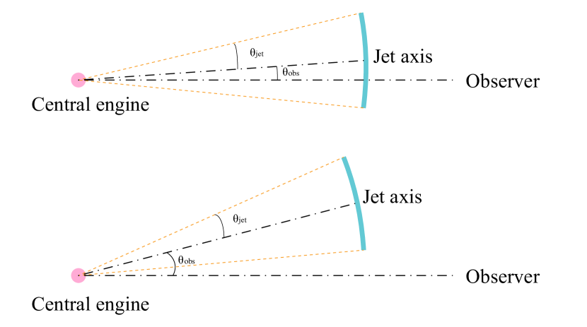
(a)

Figure 1: Geometry of our jet model. The upper panel shows the case for an on-axis jet, where $\theta_{\rm{jet}}\geq\theta_{\rm{obs}}$. The lower panel shows an off-axis jet with $\theta_{\rm{jet}}<\theta_{\rm{obs}}$.

Usually, the light curve of a single GRB pulse is composed of a fast rising phase and an exponential decay phase (Li & Zhang, 2021). Complicated processes may be involved in the prompt GRB phase, such as the hydrodynamics of the outflow and the cooling of electrons (Zhang et al., 2007). Analytical solutions will be too difficult to derive if these ingredients are included. Especially in the context of the internal shock model, our assumption of a small $\delta t$ implies that the pulse is simply produced by the collision of two very thin shells. In realistic cases, a reverse shock may form and propagate backward during the collision. The pulse profile could then be affected by the hydrodynamics of the flow, not only by the curvature of the emitting shell. Depending on the initial distribution of the Lorentz factor, the effect can remain moderate, however, and the two-shell model we considered is approximately valid.

Electrons accelerated by internal shocks should be in the fast-cooling regime. They will follow a distribution of (Geng et al., 2018)

$$\frac{dN_{e}}{d\gamma^{\prime}_{\rm{e}}}=\left\{\begin{array}[]{ll}C_{1}\gamma^{\prime-2}_{\rm{e}},&\gamma^{\prime}_{\rm{m}}<\gamma^{\prime}_{\rm{e}}<\gamma^{\prime}_{\rm{inj}},\\ C_{2}\gamma^{\prime-p-1}_{\rm{e}},&\gamma^{\prime}_{\rm{inj}}<\gamma^{\prime}_{\rm{e}}<\gamma^{\prime}_{\rm{max}},\end{array}\right.$$ (2)

with

$$\begin{array}[]{c}C_{1}=N_{\rm{e}}\left[\gamma^{\prime-1}_{\rm{m}}-\left(1-\frac{1}{p}\right)\gamma^{\prime-1}_{\rm{inj}}-\frac{1}{p}\left(\frac{\gamma^{\prime}_{\rm{inj}}}{\gamma^{\prime}_{\rm{max}}}\right)^{p}\gamma^{\prime-1}_{\rm{inj}}\right]^{-1},\\ C_{2}=C_{1}\gamma^{\prime-p-1}_{\rm{inj}},\end{array}$$ (3)

where $\gamma^{\prime}_{\rm{e}}$ is the Lorentz factor of electrons, and $N_{\rm{e}}$ is their total number. The spectral index $p$ usually ranges from $2$ – $3$ (Huang et al., 2000). $\gamma^{\prime}_{\rm{m}}$ and $\gamma^{\prime}_{\rm{max}}$ are the minimum and maximum electron Lorentz factor, respectively. $\gamma^{\prime}_{\rm{m}}$ is less than the initial Lorentz factor of the injected electrons ($\gamma^{\prime}_{\rm{inj}}$) in the fast-cooling regime (Burgess et al., 2020), while $\gamma^{\prime}_{\rm{max}}$ can be calculated approximately as $\gamma^{\prime}_{\rm{max}}\sim 10^{8}(\frac{B^{\prime}}{1G})^{-0.5}$ (Dai & Lu, 1999; Huang et al., 2000), where $B^{\prime}$ is the magnetic field strength in the comoving frame.

In the comoving frame, the synchrotron radiation power of these electrons at frequency $\nu^{\prime}$ is (Rybicki & Lightman, 1979)

$$P^{\prime}_{\nu^{\prime}}\left(N_{\rm{e}}\right)=\frac{\sqrt{3}e^{3}B^{\prime}}{m_{\rm{e}}c^{2}}\int_{\gamma^{\prime}_{\rm{m}}}^{\gamma^{\prime}_{\rm{max}}}\left(\frac{dN_{\rm{e}}}{d\gamma^{\prime}_{e}}\right)F\left(\frac{\nu^{\prime}}{\nu_{\rm{c}}^{\prime}}\right)d\gamma^{\prime}_{\rm{e}},$$ (4)

where $e$ is the electron charge, and $m_{\rm{e}}$ is the electron mass. $\nu_{\rm{c}}^{\prime}=3\gamma^{\prime 2}_{\rm{e}}eB^{\prime}/4\pi m_{\rm{e}}c$ and $F(x)=x\int_{x}^{+\infty}K_{5/3}(k)dk$, where $x=\frac{\nu^{\prime}}{\nu_{\rm{c}}^{\prime}}$ and $K_{5/3}(k)$ is the Bessel function.

In the local burst frame, the angular distribution of the radiation power is (Rybicki & Lightman, 1979)

$$\frac{dP_{\nu}}{d\Omega}=\mathcal{D}^{3}\frac{dP^{\prime}_{\nu^{\prime}}}{d\Omega^{\prime}}=\mathcal{D}^{3}\frac{P^{\prime}_{\nu^{\prime}}}{4\pi},$$ (5)

where $\mathcal{D}=1/[\gamma(1-\beta\cos\theta)]$ is the Doppler factor, and $\nu^{\prime}=(1+z)\nu_{\mathrm{obs}}/\mathcal{D}$. The radiation is assumed to be isotropic in the comoving frame.

Due to the different light-traveling time, photons emitted at different angles ($\theta$) will be received by the observer at different times. This is called the curvature effect. Summing up the contribution from the whole jet, we can obtain the observed $\gamma$-ray light curve. We first consider a time interval of $\Delta t$ in the local burst frame. It corresponds to a thin ring of $[\theta,\theta+\Delta\theta]$. When the electrons are uniformly distributed in the shell, the number of electrons in the ring is

$$N_{\theta}=\frac{\phi(\theta)\sin\theta\Delta\theta}{2\pi f_{\rm{b}}}N_{\rm{tot}},$$ (6)

where $f_{\rm{b}}=1-\cos\theta_{\rm{jet}}$ is the beaming factor, $N_{\rm{tot}}$ is the total number of electrons in the shell, and $\phi(\theta)$ is the annular angle of the ring. $N_{\rm{tot}}$ can be derived from the isotropic-equivalent mass of the shell $m_{\rm{sh}}$ as $N_{\rm{tot}}=2\pi f_{\rm{b}}m_{\rm{sh}}/m_{\rm{p}}$, where $m_{\rm{p}}$ is the mass of the proton. The annular angle $\phi(\theta)$ takes the form of

$$\phi(\theta)=\left\{\begin{array}[]{ll}2\pi,&\theta\leq|\theta_{\rm{obs}}-\theta_{\rm{jet}}|,\\ 2\arccos(\frac{\cos\theta_{\rm{jet}}-\cos\theta_{\rm{obs}}\cos\theta}{\sin\theta_{\rm{obs}}\sin\theta}),&\theta>|\theta_{\rm{obs}}-\theta_{\rm{jet}}|.\\ \end{array}\right.$$ (7)

Since the radiation process only lasts for a short interval of $\delta t$, the energy emitted into one unit solid angle is

$$\frac{\Delta E_{\nu}}{d\Omega}=\mathcal{D}^{3}\frac{P^{\prime}_{\nu^{\prime}}\delta t}{4\pi}.$$ (8)

This energy corresponds to a duration of $\Delta t=r\sin\theta\Delta\theta/c$ in the local burster frame. The luminosity is then $L_{\nu}=\Delta E_{\nu}/\Delta t$. For an observer at distance $D_{\rm{L}}$, the observed flux at $t_{\rm{obs}}(\theta)$ should be $F_{\nu}(\theta)=(1+z)L_{\nu}/4\pi D_{\rm{L}}^{2}$, that is,

$$F_{\nu}(\theta)=\frac{(1+z)}{4\pi D_{\rm{L}}^{2}}\frac{c}{r}\frac{\mathcal{D}^{3}P^{\prime}_{\nu^{\prime}}(N_{\theta})\delta t}{\sin\theta\Delta\theta}.$$ (9)

The total isotropic energy can be calculated as

$$E_{\rm{iso}}=\frac{4\pi D_{\rm{L}}^{2}}{(1+z)}\int_{0}^{t_{\rm{end}}}\int_{\nu_{1}/(1+z)}^{\nu_{2}/(1+z)}F_{\nu}(\theta)d\nu dt_{\rm{obs}}(\theta),$$ (10)

where $t_{\rm{end}}=r(\cos\theta_{1}-\cos(\theta_{\rm{jet}}+\theta_{\rm{obs}}))(1+z)/c$ is the end time of the pulse in the observer frame. The isotropic peak luminosity is

$$L_{\rm{p}}=4\pi D_{\rm{L}}^{2}\int_{\nu_{1}/(1+z)}^{\nu_{2}/(1+z)}F_{\nu}(\theta_{\rm{p}})d\nu,$$ (11)

where $\theta_{\rm{p}}$ is the angle corresponding to the peak time of the light curve. The peak photon energy $E_{\rm{p}}$ can be derived from the time-integrated spectrum. In the next section, we present an analytic derivation for the prompt $\gamma$-ray emission, paying special attention to the three parameters $E_{\rm{iso}}$, $L_{\rm{p}}$, and $E_{\rm{p}}$.

3 Analytic derivation of $E_{\rm{p}}$, $E_{\rm{iso}}$, and $L_{\rm{p}}$

We first consider the on-axis cases. From Equations 1 and 10, we can derive $E_{\rm{iso}}$ as

$$E_{\rm{iso}} =c\delta t\int_{0}^{t_{\rm{end}}}\int_{\nu_{1}/(1+z)}^{\nu_{2}/(1+z)}\frac{\mathcal{D}^{3}P^{\prime}_{\nu^{\prime}}(N_{\theta})}{r\sin\theta\Delta\theta}d\nu dt_{\rm{obs}}(\theta)$$ (12)

$$\propto\int_{\theta_{1}}^{\theta_{2}}\int_{\nu_{1}/(1+z)}^{\nu_{2}/(1+z)}\frac{(1+z)\frac{r}{c}\sin\theta d\theta P^{\prime}_{\nu^{\prime}}(N_{\theta})}{\gamma^{3}(1-\beta\cos\theta)^{3}r\sin\theta\Delta\theta}d\nu$$

$$\propto\frac{1}{\gamma^{3}}\int_{\theta_{1}}^{\theta_{2}}\frac{1}{(1-\beta\cos\theta)^{3}}\int_{\nu_{1}/(1+z)}^{\nu_{2}/(1+z)}(1+z)\frac{P^{\prime}_{\nu^{\prime}}(N_{\theta})}{\Delta\theta}d\nu d\theta,$$

where $\theta_{2}=\theta_{\rm{jet}}+\theta_{\rm{obs}}$. Further combining Equation 4, we have

$$E_{\rm{iso}}\propto\frac{(1+z)B^{\prime}}{\gamma^{3}}\frac{\sqrt{3}e^{3}}{m_{\rm{e}}c^{2}} \int_{\theta_{1}}^{\theta_{2}}\frac{1}{(1-\beta\cos\theta)^{3}}\int_{\nu_{1}/(1+z)}^{\nu_{2}/(1+z)}\frac{1}{\Delta\theta}$$ (13)

$$\int_{\gamma^{\prime}_{\rm{m}}}^{\gamma^{\prime}_{\rm{max}}}\left(\frac{dN_{\theta}}{d\gamma^{\prime}_{e}}\right)F\left(\frac{\nu^{\prime}}{\nu_{\rm{c}}^{\prime}}\right)d\gamma^{\prime}_{\rm{e}}d\nu d\theta.$$

We note that $C_{1}$ in Equation 3 is largely dependent on $\gamma^{\prime}_{\rm{m}}$ and $\gamma^{\prime}_{\rm{inj}}$. In this study, a simple case of $\gamma^{\prime}_{\rm{m}}=\gamma^{\prime}_{\rm{inj}}/10$ is assumed, which naturally leads to $C_{1}\propto\gamma^{\prime}_{\rm{inj}}$. Then with Equations 2, 3, and 6, we can further obtain

$$E_{\rm{iso}} \propto\frac{(1+z)B^{\prime}}{\gamma^{3}}\int_{\theta_{1}}^{\theta_{2}}\frac{1}{(1-\beta\cos\theta)^{3}}\int_{\nu_{1}/(1+z)}^{\nu_{2}/(1+z)}\frac{1}{\Delta\theta}$$ (14)

$$\quad\left[\int_{\gamma^{\prime}_{\rm{m}}}^{\gamma^{\prime}_{\rm{inj}}}N_{\theta}\gamma^{\prime}_{\rm{inj}}\gamma^{\prime-2}_{\rm{e}}F\left(\frac{\nu^{\prime}}{\nu_{\rm{c}}^{\prime}}\right)d\gamma^{\prime}_{\rm{e}}+\right.$$

$$\quad\left.\int_{\gamma^{\prime}_{\rm{inj}}}^{\gamma^{\prime}_{\rm{max}}}N_{\theta}\gamma^{\prime p}_{\rm{inj}}\gamma^{\prime-p-1}_{\rm{e}}F\left(\frac{\nu^{\prime}}{\nu_{\rm{c}}^{\prime}}\right)d\gamma^{\prime}_{\rm{e}}\right]d\nu d\theta$$

$$\propto\frac{(1+z)B^{\prime}m_{\rm{sh}}}{\gamma^{3}}\int_{\theta_{1}}^{\theta_{2}}\frac{\phi(\theta)\sin\theta}{(1-\beta\cos\theta)^{3}}$$

$$\quad\left[\int_{\nu_{1}/(1+z)}^{\nu_{2}/(1+z)}\int_{\gamma^{\prime}_{\rm{m}}}^{\gamma^{\prime}_{\rm{inj}}}\gamma^{\prime}_{\rm{inj}}\gamma^{\prime-2}_{\rm{e}}F\left(\frac{\nu^{\prime}}{\nu_{\rm{c}}^{\prime}}\right)d\gamma^{\prime}_{\rm{e}}d\nu+\right.$$

$$\quad\left.\int_{\nu_{1}/(1+z)}^{\nu_{2}/(1+z)}\int_{\gamma^{\prime}_{\rm{inj}}}^{\gamma^{\prime}_{\rm{max}}}\gamma^{\prime p}_{\rm{inj}}\gamma^{\prime-p-1}_{\rm{e}}F\left(\frac{\nu^{\prime}}{\nu_{\rm{c}}^{\prime}}\right)d\gamma^{\prime}_{\rm{e}}d\nu\right]d\theta.$$

For an on-axis observer, most of the observed photons are emitted by electrons within a small angle around the line of sight. According to Equation 7, it is safe for us to simply take $\phi(\theta)$ as $2\pi$. Changing the integral order in Equation 14, we obtain

$$E_{\rm{iso}} \propto\frac{(1+z)B^{\prime}m_{\rm{sh}}}{\gamma^{3}}\int_{\theta_{1}}^{\theta_{2}}\frac{\sin\theta}{(1-\beta\cos\theta)^{3}}$$ (15)

$$\quad\left[\int_{\gamma^{\prime}_{\rm{m}}}^{\gamma^{\prime}_{\rm{inj}}}\int_{\nu_{1}/(1+z)}^{\nu_{2}/(1+z)}\gamma^{\prime}_{\rm{inj}}\gamma^{\prime-2}_{\rm{e}}F\left(\frac{\nu^{\prime}}{\nu_{\rm{c}}^{\prime}}\right)d\gamma^{\prime}_{\rm{e}}d\nu+\right.$$

$$\quad\left.\int_{\gamma^{\prime}_{\rm{inj}}}^{\gamma^{\prime}_{\rm{max}}}\int_{\nu_{1}/(1+z)}^{\nu_{2}/(1+z)}\gamma^{\prime p}_{\rm{inj}}\gamma^{\prime-p-1}_{\rm{e}}F\left(\frac{\nu^{\prime}}{\nu_{\rm{c}}^{\prime}}\right)d\gamma^{\prime}_{\rm{e}}d\nu\right]d\theta$$

$$\propto\frac{(1+z)B^{\prime}m_{\rm{sh}}}{\gamma^{3}}\int_{\theta_{1}}^{\theta_{2}}\frac{\sin\theta}{(1-\beta\cos\theta)^{3}}$$

$$\quad\left[\int_{\gamma^{\prime}_{\rm{m}}}^{\gamma^{\prime}_{\rm{inj}}}\gamma^{\prime}_{\rm{inj}}\gamma^{\prime-2}_{\rm{e}}\frac{\gamma^{\prime 2}_{\rm{e}}B^{\prime}}{(1+z)\gamma(1-\beta\cos\theta)}\right.$$

$$\quad\int_{\frac{\nu^{\prime}_{1}}{\nu^{\prime}_{\rm{c}}}/(1+z)}^{\frac{\nu^{\prime}_{2}}{\nu^{\prime}_{\rm{c}}}/(1+z)}F\left(\frac{\nu^{\prime}}{\nu_{\rm{c}}^{\prime}}\right)d(\frac{\nu^{\prime}_{1}}{\nu^{\prime}_{\rm{c}}})d\gamma^{\prime}_{\rm{e}}+$$

$$\quad\int_{\gamma^{\prime}_{\rm{inj}}}^{\gamma^{\prime}_{\rm{max}}}\gamma^{\prime p}_{\rm{inj}}\gamma^{\prime-p-1}_{\rm{e}}\frac{\gamma^{\prime 2}_{\rm{e}}B^{\prime}}{(1+z)\gamma(1-\beta\cos\theta)}$$

$$\quad\left.\int_{\frac{\nu^{\prime}_{1}}{\nu^{\prime}_{\rm{c}}}/(1+z)}^{\frac{\nu^{\prime}_{2}}{\nu^{\prime}_{\rm{c}}}/(1+z)}F\left(\frac{\nu^{\prime}}{\nu_{\rm{c}}^{\prime}}\right)d(\frac{\nu^{\prime}_{1}}{\nu^{\prime}_{\rm{c}}})d\gamma^{\prime}_{\rm{e}}\right]d\theta$$

$$\propto\frac{B^{\prime 2}m_{\rm{sh}}}{\gamma^{4}}\int_{\theta_{1}}^{\theta_{2}}\frac{\sin\theta}{(1-\beta\cos\theta)^{4}}\left[\int_{\gamma^{\prime}_{\rm{m}}}^{\gamma^{\prime}_{\rm{inj}}}k_{0}\gamma^{\prime}_{\rm{inj}}d\gamma^{\prime}_{\rm{e}}+\right.$$

$$\ \ \ \ \ \left.\int_{\gamma^{\prime}_{\rm{inj}}}^{\gamma^{\prime}_{\rm{max}}}k_{0}\gamma^{\prime p}_{\rm{inj}}\gamma^{\prime-p+1}_{\rm{e}}d\gamma^{\prime}_{\rm{e}}\right]d\theta.$$

In the last step above, the integral of $F\left(\frac{\nu^{\prime}}{\nu_{\rm{c}}^{\prime}}\right)$ has been simplified as a constant ($k_{0}$). Equation 15 can be further reduced as

$$E_{\rm{iso}} \propto\frac{B^{\prime 2}m_{\rm{sh}}}{\gamma^{4}}\int_{\theta_{1}}^{\theta_{2}}\frac{\sin\theta}{(1-\beta\cos\theta)^{4}}\left[k_{1}\gamma^{\prime}_{\rm{inj}}(\gamma^{\prime}_{\rm{inj}}-\gamma^{\prime}_{\rm{m}})+\right.$$ (16)

$$\quad\left.k_{2}\gamma^{\prime p}_{\rm{inj}}(\gamma^{\prime 2-p}_{\rm{inj}}-\gamma^{\prime 2-p}_{\rm{max}})\right]d\theta$$

$$\propto\frac{B^{\prime 2}\gamma^{\prime 2}_{\rm{inj}}m_{\rm{sh}}}{\gamma^{4}}\int_{\theta_{1}}^{\theta_{2}}\frac{\sin\theta}{(1-\beta\cos\theta)^{4}}d\theta,$$

where $k_{1}$ and $k_{2}$ are integration constants. When $\theta<<1$ and $\beta\sim 1$, we have $1/(1-\beta\cos\theta)\sim 2\gamma^{2}/(\theta^{2}\gamma^{2}+1)$. The integral in Equation 16 can therefore be approximated as

$$\int_{\theta_{1}}^{\theta_{2}}\frac{\sin\theta}{(1-\beta\cos\theta)^{4}}d\theta \approx\int_{\theta_{1}}^{\theta_{2}}\frac{\theta}{(\frac{\theta^{2}\gamma^{2}+1}{2\gamma^{2}})^{4}}d\theta$$ (17)

$$=16\gamma^{6}\int_{\theta_{1}}^{\theta_{2}}\frac{\theta\gamma}{(\theta^{2}\gamma^{2}+1)^{4}}d(\theta\gamma)$$

$$=16\gamma^{6}\left.-\frac{1}{6((\theta\gamma)^{2}+1)^{3}}\right|_{\theta_{1}=0}^{\theta_{2}=\theta_{\rm{obs}}+\theta_{\rm{jet}}\gg\frac{1}{\gamma}}$$

$$\approx\frac{8}{3}\gamma^{6}.$$

Finally, combining Equations 16 and 17, it is easy to obtain $E_{\rm{iso}}\propto\gamma^{\prime 2}_{\rm{inj}}m_{\rm{sh}}B^{\prime 2}\gamma^{2}$.

Now we derive the peak luminosity of $L_{\rm{p}}$. Since the main difference between Equations 10 and 11 is the integral of time, we can first consider the luminosity corresponding to a particular angle $\theta$ as

$$L(\theta) \propto\frac{B^{\prime 2}\gamma^{\prime 2}_{\rm{inj}}m_{\rm{sh}}}{r\gamma^{4}}\frac{1}{(1-\beta\cos\theta)^{4}}$$ (18)

$$\propto\frac{B^{\prime 2}\gamma^{\prime 2}_{\rm{inj}}m_{\rm{sh}}}{d\gamma^{6}}\frac{1}{(\frac{\theta^{2}\gamma^{2}+1}{2\gamma^{2}})^{4}}$$

$$\propto\frac{B^{\prime 2}\gamma^{\prime 2}_{\rm{inj}}m_{\rm{sh}}\gamma^{2}}{d}\frac{1}{(\theta^{2}\gamma^{2}+1)^{4}}.$$

The flux peaks at $\theta_{\rm{p}}\sim 0$, thus the peak luminosity is $L_{\rm{p}}=L(\theta_{\rm{p}})\propto\gamma^{\prime 2}_{\rm{inj}}m_{\rm{sh}}d^{-1}B^{\prime 2}\gamma^{2}$.

The peak photon energy in the observer frame can be derived by considering the standard synchrotron emission mechanism,

$$E_{\rm{p,obs}} \approx\frac{1}{(1+z)}\frac{1}{\gamma(1-\beta\cos\theta)}\frac{3heB^{\prime}}{4\pi m_{e}c}\gamma^{\prime 2}_{\rm{inj}}$$ (19)

$$\propto\frac{B^{\prime}\gamma^{\prime 2}_{\rm{inj}}}{(1+z)}\frac{2\gamma}{\theta^{2}\gamma^{2}+1}$$

$$\approx\frac{B^{\prime}\gamma^{\prime 2}_{\rm{inj}}}{(1+z)}\frac{2\gamma}{\theta_{\rm{p}}^{2}\gamma^{2}+1}$$

$$\propto\frac{1}{(1+z)}\gamma B^{\prime}\gamma^{\prime 2}_{\rm{inj}}.$$

Therefore, the peak photon energy in the comoving frame is $E_{\rm{p}}=(1+z)E_{\rm{p,obs}}\propto\gamma^{\prime 2}_{\rm{inj}}B^{\prime}\gamma$.

Next, we consider the off-axis cases. Again, we first focus on $L_{\rm{p}}$. For an off-axis jet, the main difference is that $\phi(\theta)$ can no longer be taken as $2\pi$ . Instead, it should be calculated as $\phi(\theta)\equiv 2\arccos(\frac{\cos\theta_{\rm{jet}}-\cos\theta_{\rm{obs}}\cos\theta}{\sin\theta_{\rm{obs}}\sin\theta})$. Equation 18 now becomes

$$L(\theta)\propto\frac{B^{\prime 2}\gamma^{\prime 2}_{\rm{inj}}m_{\rm{sh}}}{d\gamma^{6}}\frac{1}{(1-\beta\cos\theta)^{4}}2\arccos(\frac{\cos\theta_{\rm{jet}}-\cos\theta_{\rm{obs}}\cos\theta}{\sin\theta_{\rm{obs}}\sin\theta}).$$ (20)

Here $\theta\in(\theta_{\rm{obs}}-\theta_{\rm{jet}},\theta_{\rm{obs}}+\theta_{\rm{jet}})$. We define $R(\theta)=\frac{\cos\theta_{\rm{jet}}-\cos\theta_{\rm{obs}}\cos\theta}{\sin\theta_{\rm{obs}}\sin\theta}$. Then it is obvious that $R(\theta)\in(0,1)$, which leads to the approximation $\arccos(R(\theta))\sim\sqrt{2}\sqrt{1-R(\theta)}$. We note that $R(\theta)$ can be simplified as

$$R(\theta) =\frac{\cos\theta_{\rm{jet}}-\cos\theta_{\rm{obs}}\cos\theta}{\sin\theta_{\rm{obs}}\sin\theta}$$ (21)

$$\approx\frac{1-\theta_{\rm{jet}}^{2}/2-(1-\theta_{\rm{obs}}^{2}/2)(1-\theta^{2}/2)}{\theta_{\rm{obs}}\theta}$$

$$\approx\frac{\theta_{\rm{obs}}^{2}-\theta_{\rm{jet}}^{2}+\theta^{2}}{2\theta_{\rm{obs}}\theta}.$$

When $\theta>\frac{1}{\gamma}$, we have $\frac{1}{(1-\beta\cos\theta)^{4}}\sim\frac{16\gamma^{8}}{(\theta^{2}\gamma^{2}+1)^{4}}\sim\frac{16}{\theta^{8}}$. Combining Equations 20 and 21, we obtain

$$L(\theta) \propto\frac{B^{\prime 2}\gamma^{\prime 2}_{\rm{inj}}m_{\rm{sh}}}{d\gamma^{6}}\frac{1}{\theta^{8}}\sqrt{1-R(\theta)}$$ (22)

$$\propto\frac{B^{\prime 2}\gamma^{\prime 2}_{\rm{inj}}m_{\rm{sh}}}{d\gamma^{6}}\frac{1}{\theta^{8}}\sqrt{\frac{\theta_{\rm{jet}}^{2}-(\theta_{\rm{obs}}-\theta)^{2}}{2\theta_{\rm{obs}}\theta}}.$$

In this case, $L_{\rm{p}}$ will peak at $\theta_{\rm{p}}=\frac{1}{15}(16\theta_{\rm{obs}}-\sqrt{255\theta_{\rm{jet}}^{2}+\theta_{\rm{obs}}^{2}})\sim\frac{16}{15}(\theta_{\rm{obs}}-\theta_{\rm{jet}})$. We note that the condition of $\theta_{\rm{p}}>\frac{1}{\gamma}$ leads to $\frac{16}{15}(\theta_{\rm{obs}}-\theta_{\rm{jet}})>\frac{1}{\gamma}$. Under this condition, $L_{\rm{p}}$ can be further written as

$$L_{\rm{p}} \propto\frac{B^{\prime 2}\gamma^{\prime 2}_{\rm{inj}}m_{\rm{sh}}}{d\gamma^{6}}\frac{1}{\theta_{\rm{p}}^{8}}\sqrt{\frac{\theta_{\rm{jet}}^{2}-(\theta_{\rm{obs}}-\theta_{\rm{p}})^{2}}{2\theta_{\rm{obs}}\theta_{\rm{p}}}}$$ (23)

$$\propto\frac{B^{\prime 2}\gamma^{\prime 2}_{\rm{inj}}m_{\rm{sh}}}{d\gamma^{6}}\frac{1}{\theta_{\rm{p}}^{8.5}}\sqrt{\frac{\theta_{\rm{jet}}^{2}-(\theta_{\rm{obs}}-\theta_{\rm{p}})^{2}}{2\theta_{\rm{obs}}}}$$

$$\propto\frac{B^{\prime 2}\gamma^{\prime 2}_{\rm{inj}}m_{\rm{sh}}}{d\gamma^{6}}(\theta_{\rm{obs}}-\theta_{\rm{jet}})^{-8.5}I(\theta_{\rm{obs}},\theta_{\rm{jet}},\theta=\theta_{\rm{p}}).$$

The last factor is $I(\theta_{\rm{obs}},\theta_{\rm{jet}},\theta=\theta_{\rm{p}})=\sqrt{\frac{\theta_{\rm{jet}}^{2}-(\theta_{\rm{obs}}-\theta_{\rm{p}})^{2}}{2\theta_{\rm{obs}}}}$. Its effect is not important compared with $(\theta_{\rm{obs}}-\theta_{\rm{jet}})^{-8.5}$, and therefore, we ignore this factor for simplicity. Finally, we obtain $L_{\rm{p}}\propto\gamma^{\prime 2}_{\rm{inj}}m_{\rm{sh}}d^{-1}B^{\prime 2}\gamma^{-6}(\theta_{\rm{obs}}-\theta_{\rm{jet}})^{-8.5}$.

Now we continue to calculate $E_{\rm{iso}}$. Since most of the $\gamma$-ray energy is released in the decay stage of the light curve, we only need to integrate the energy over a $\theta$ ranging from $\theta_{\rm{p}}$ to $\theta_{\rm{obs}}+\theta_{\rm{jet}}$, that is,

$$E_{\rm{iso}} \propto\frac{B^{\prime 2}\gamma^{\prime 2}_{\rm{inj}}m_{\rm{sh}}}{\gamma^{4}}\int_{\theta_{\rm{p}}}^{\theta_{\rm{obs}}+\theta_{\rm{jet}}}\frac{\sin\theta}{(1-\beta\cos\theta)^{4}}$$ (24)

$$\quad 2\arccos(\frac{\cos\theta_{\rm{jet}}-\cos\theta_{\rm{obs}}\cos\theta}{\sin\theta_{\rm{obs}}\sin\theta})d\theta$$

$$\propto\frac{B^{\prime 2}\gamma^{\prime 2}_{\rm{inj}}m_{\rm{sh}}}{\gamma^{4}}\int_{\theta_{\rm{p}}}^{\theta_{\rm{obs}}+\theta_{\rm{jet}}}\frac{1}{\theta^{7}}\sqrt{\frac{\theta_{\rm{jet}}^{2}-(\theta_{\rm{obs}}-\theta)^{2}}{2\theta_{\rm{obs}}\theta}}d\theta$$

$$\propto\frac{B^{\prime 2}\gamma^{\prime 2}_{\rm{inj}}m_{\rm{sh}}}{\gamma^{4}}\int_{\theta_{\rm{p}}}^{\theta_{\rm{obs}}+\theta_{\rm{jet}}}\frac{1}{\theta^{7.5}}I(\theta_{\rm{obs}},\theta_{\rm{jet}},\theta)d\theta$$

$$\approx\frac{B^{\prime 2}\gamma^{\prime 2}_{\rm{inj}}m_{\rm{sh}}}{\gamma^{4}}\int_{\theta_{\rm{p}}}^{\theta_{\rm{obs}}+\theta_{\rm{jet}}}\frac{1}{\theta^{7.5}}I(\theta_{\rm{obs}},\theta_{\rm{jet}},\theta=\theta_{p})d\theta$$

$$\propto\frac{B^{\prime 2}\gamma^{\prime 2}_{\rm{inj}}m_{\rm{sh}}}{\gamma^{4}}I(\theta_{\rm{obs}},\theta_{\rm{jet}},\theta=\theta_{p})\left.\theta^{-6.5}\right|_{\theta_{\rm{p}}}^{\theta_{\rm{obs}}+\theta_{\rm{jet}}}$$

$$\propto\frac{B^{\prime 2}\gamma^{\prime 2}_{\rm{inj}}m_{\rm{sh}}}{\gamma^{4}}\theta_{\rm{p}}^{-6.5}.$$

Here the value of $I(\theta_{\rm{obs}},\theta_{\rm{jet}},\theta)$ will not change significantly in the range from $\theta_{\rm{p}}$ to $\theta_{\rm{obs}}+\theta_{\rm{jet}}$. Hence it can be taken as a constant for simplicity. Since $\theta_{\rm{p}}\sim\frac{16}{15}(\theta_{\rm{obs}}-\theta_{\rm{jet}})$, we obtain the result as $E_{\rm{iso}}\propto\gamma^{\prime 2}_{\rm{inj}}m_{\rm{sh}}B^{\prime 2}\gamma^{-4}(\theta_{\rm{obs}}-\theta_{\rm{jet}})^{-6.5}$.

Finally, we calculate $E_{\rm{p}}$. Similar to Equation 19, the peak energy in the rest frame is

$$E_{\rm{p}} \approx B^{\prime}\gamma^{\prime 2}_{\rm{inj}}\frac{2\gamma}{\theta_{\rm{p}}^{2}\gamma^{2}+1}$$ (25)

$$\approx B^{\prime}\gamma^{\prime 2}_{\rm{inj}}\frac{2\gamma}{(\theta_{\rm{obs}}-\theta_{\rm{jet}})^{2}\gamma^{2}}$$

$$\propto\frac{B^{\prime}\gamma^{\prime 2}_{\rm{inj}}}{\gamma}(\theta_{\rm{obs}}-\theta_{\rm{jet}})^{-2}.$$

We see that $E_{\rm{p}}\propto\gamma^{\prime 2}_{\rm{inj}}B^{\prime}\gamma^{-1}(\theta_{\rm{obs}}-\theta_{\rm{jet}})^{-2}$.

To summarize, in the on-axis cases, we have

$$\begin{array}[]{ll}E_{\rm{p}}&\propto\gamma^{\prime 2}_{\rm{inj}}B^{\prime}\gamma,\\ E_{\rm{iso}}&\propto\gamma^{\prime 2}_{\rm{inj}}m_{\rm{sh}}B^{\prime 2}\gamma^{2},\\ L_{\rm{p}}&\propto\gamma^{\prime 2}_{\rm{inj}}m_{\rm{sh}}d^{-1}B^{\prime 2}\gamma^{2},\end{array}$$ (26)

while in the off-axis cases ($\theta_{\rm{obs}}-\theta_{\rm{jet}}>1/\gamma$), we obtain

$$\begin{array}[]{ll}E_{\rm{p}}&\propto\gamma^{\prime 2}_{\rm{inj}}B^{\prime}\gamma^{-1}(\theta_{\rm{obs}}-\theta_{\rm{jet}})^{-2},\\ E_{\rm{iso}}&\propto\gamma^{\prime 2}_{\rm{inj}}m_{\rm{sh}}B^{\prime 2}\gamma^{-4}(\theta_{\rm{obs}}-\theta_{\rm{jet}})^{-6.5},\\ L_{\rm{p}}&\propto\gamma^{\prime 2}_{\rm{inj}}m_{\rm{sh}}d^{-1}B^{\prime 2}\gamma^{-6}(\theta_{\rm{obs}}-\theta_{\rm{jet}})^{-8.5}.\end{array}$$ (27)

The equations derived above are very simple but intriguing. There are eight input parameters in our model: $\gamma$, $B^{\prime}$, $\gamma^{\prime}_{\rm{inj}}$, $\theta_{\rm{jet}}$, $\theta_{\rm{obs}}$, $m_{\rm{sh}}c^{2}$, $d$, and the electron spectral index $p$. Seven of them are closely related to the prompt emission parameters of $E_{\rm{p}}$, $E_{\rm{iso}}$, and $L_{\rm{p}}$, while $p$ is largely irrelevant. Of all the input parameters, $\gamma$ plays the most important role in affecting the observed spectral peak energies and fluxes for on-axis cases (Ghirlanda et al., 2018). Usually, $\gamma$ may vary in a wide range for different GRBs, from lower than 100 to more than 1000. In contrast, $\gamma^{\prime}_{\rm{inj}}$ and $m_{\rm{sh}}$ only vary in much narrower ranges. Taking $\gamma^{\prime}_{\rm{inj}}$ and $m_{\rm{sh}}$ approximately as constants, from Equation 26, we can easily derive the on-axis Amati relation as $E_{\rm{p}}\propto E_{\rm{iso}}^{0.5}$ and the on-axis Yonetoku relation as $E_{\rm{p}}\propto L_{\rm{p}}^{0.5}$. In both relations, the power-law indices are 0.5, which is largely consistent with observations (Nava et al., 2012; Demianski et al., 2017).

In the off-axis cases, previous studies mainly focused on the effect of the variation of the viewing angle among different GRBs. Consequently, the power-law index of the off-axis Amati relation is derived as $1/3$ based on the sharp-edge homogeneous jet geometry (Granot et al., 2002; Ramirez-Ruiz et al., 2005). Here, from our Equation 27, we see that $E_{\rm{iso}}$ and $L_{\rm{p}}$ sensitively depend on both the viewing angle and the Lorentz factor. This indicates that both $\gamma$ and $\theta_{\rm{obs}}$ are important parameters that will affect the slope of the Amati relation and the Yonetoku relation. In Equation 27, if only the variation of the viewing angle is considered (i.e., the indices of $(\theta_{\rm{obs}}-\theta_{\rm{jet}})$ in Equation 27 are taken into account, but the item of $\gamma$ is omitted), an index of $4/13$ will be derived for the off-axis Amati relation, which is very close to the previous result of $1/3$. When the combined effect of varying $\gamma$ and $\theta_{\rm{obs}}$ is included, the off-axis Amati relation is derived as $E_{\rm{p}}\propto E_{\rm{iso}}^{1/4\sim 4/13}$, and the corresponding off-axis Yonetoku relation is $E_{\rm{p}}\propto L_{\rm{p}}^{1/6\sim 4/17}$. The power-law indices become smaller than in the on-axis cases.

4 Numerical results

Some approximations have been made in deriving Equations 26 and 27. In this section, we carry out numerical simulations to confirm whether the above analytical derivations are correct. For convenience, a set of standard values were taken for the eight input parameters in our simulations, as shown in Table 1. When studying the effect of one particular parameter, we only changed this parameter, but fixed all other parameters at the standard values.

Table 1: Standard values assumed for the eight input parameters

$\gamma$	$B^{\prime}$	$\gamma^{\prime}_{\rm{inj}}$	$\theta_{\rm{jet}}$	$\theta_{\rm{obs}}$	$p$	$m_{\rm{sh}}c^{2}$	$d$
	(G)		(rad)	(rad)		(erg)	(cm)
100	10	1e5	0.1	0.0(0.2)	2.5	1e52	1e10

To examine the correctness of our analytical derivations, we chose one input parameter as a variable, and standard values were taken for all other input parameters so that the dependence of $E_{\rm{p}}$, $E_{\rm{iso}}$, and $L_{\rm{p}}$ on that particular parameter can be illustrated.

We first consider the effect of the bulk Lorentz factor $\gamma$ for both on-axis and off-axis cases. Here we let $\gamma$ vary between 50 — 1000. Figure 2 shows the time-integrated spectrum obtained for different $\gamma$. The peak photon energy is correspondingly marked with a black star on the curve.

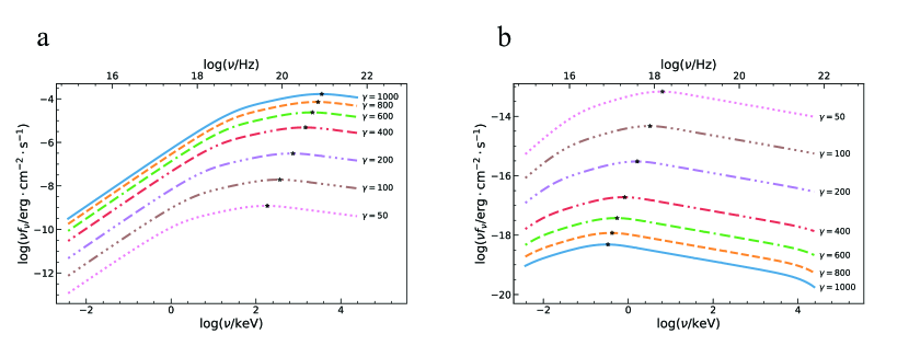
Figure 2: Time-integrated spectrum for different $\gamma$ values (marked in the figure). Panel a Spectrum of on-axis cases. Panel b Spectrum of off-axis cases. The black star on each curve marks the position of the peak energy ($E_{\rm{p}}$).

For on-axis cases ($\theta_{\rm{jet}}\geq\theta_{\rm{obs}}$), the numerical results are plotted in the left panel of Figure 2. When the value of $\gamma$ increases, the peak photon energy and the flux increase simultaneously. However, a different trend is found for the off-axis cases ($\theta_{\rm{jet}}<\theta_{\rm{obs}}$), as shown in the right panel of Figure 2. Both the flux and $E_{\rm{p}}$ decrease as $\gamma$ increases. The flux is significantly lower than that of the on-axis cases. The results are consistent with those of Farinelli et al. (2021).

Figure 2 clearly shows that both $E_{\rm{p}}$ and the flux are positively correlated with $\gamma$ in the on-axis cases, but they are negatively correlated with $\gamma$ in the off-axis cases. Next, we wish to determine the precise relation between the prompt emission parameters and the input parameters. Hence, we plot $E_{\rm{p}}$, $E_{\rm{iso}}$, and $L_{\rm{p}}$ as functions of $\gamma$, $B^{\prime}$, $\gamma^{\prime}_{\rm{inj}}$, $|\theta_{\rm{obs}}-\theta_{\rm{jet}}|$, and $p$ in Figure 3.

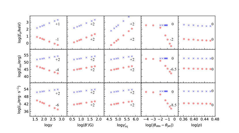
Figure 3: Numerical results showing the dependence of the prompt emission features on the input parameters. The calculated prompt emission parameters ($E_{\rm{p}}$, $E_{\rm{iso}}$, and $L_{\rm{p}}$) are plotted against the input parameters ($\gamma$, $B^{\prime}$, $\gamma^{\prime}_{\rm{inj}}$, $|\theta_{\rm{obs}}-\theta_{\rm{jet}}|$, and $p$) for both the on-axis cases (with cross symbols) and the off-axis cases (with circle symbols). For comparison, the power-law indices derived from our analytical solutions are marked correspondingly in each panel.

Generally, the simulation results are well consistent with our analytical results of Equations 26 and 27. Especially $E_{\rm{p}}$, $E_{\rm{iso}}$, and $L_{\rm{p}}$ have a positive dependence on the Lorentz factor $\gamma$ in the on-axis cases, but they have a negative dependence on $\gamma$ in the off-axis cases. It is also interesting to note that the prompt emission parameters are nearly independent of $\theta_{\rm{obs}}-\theta_{\rm{jet}}$ in the on-axis cases, since the line of sight is always within the jet cone. However, in the off-axis cases, the dependence of the prompt emission parameters on $\theta_{\rm{obs}}-\theta_{\rm{jet}}$ can be described as a two-phase behavior. When $\theta_{\rm{obs}}-\theta_{\rm{jet}}\ll 1/\gamma$, the prompt emission parameters are independent of $\theta_{\rm{obs}}-\theta_{\rm{jet}}$. When $\theta_{\rm{obs}}-\theta_{\rm{jet}}>1/\gamma$, however, they decrease sharply with the increase of $\theta_{\rm{obs}}-\theta_{\rm{jet}}$, as indicated in Equation 27. Finally, the last column of Figure 3 shows that the parameter $p$ has little impact on the prompt emission parameters.

5 Monte Carlo simulations

In this section, we perform Monte Carlo simulations to generate a large number of mock GRBs to further test the existence of the Amati relation and the Yonetoku relation. For this purpose, we performed Monte Carlo simulations as follows. First, a group of eight input parameters is generated randomly, assuming that each parameter follows a particular distribution. This group of parameters defines a mock GRB. Second, our model is applied to numerically calculate the corresponding values of $E_{\rm{p}}$, $E_{\rm{iso}}$, and $L_{\rm{p}}$ for this mock GRB. The above two steps are repeated until we obtain a large sample of mock GRBs. Finally, the mock bursts are plotted on the $E_{\rm{p}}-E_{\rm{iso}}$ plane and the $E_{\rm{p}}-L_{\rm{p}}$ plane, and a best-fit correlation is obtained for them.

For convenience, we designate the distribution function of a particular parameter $a$ as $D(a)$. Here $a$ refers to the input parameters (i.e., $\gamma$, $B^{\prime}$, $\gamma^{\prime}_{\rm{inj}}$, $\theta_{\rm{jet}}$, $\theta_{\rm{obs}}$, $p$, $m_{\rm{sh}}c^{2}$, and $d$). Three kinds of distributions are adopted in this study: (i) A normal Gaussian distribution, which is noted as $N(\mu,\sigma)$, where $\mu$ and $\sigma$ refer to the mean value and standard deviation, respectively. (ii) A uniform distribution, which is noted as $U(\rm{min},\rm{max})$, where $\rm{min}$ and $\rm{max}$ define the range of the parameter. Finally, (iii) a log-normal distribution, noted as $D(\log(a))$, which means that $\log(a)$ follows a normal Gaussian distribution of $N(\mu,\sigma)$. The detailed distribution for each of the input parameters adopted in our Monte Carlo simulations is described below.

The ranges of some input parameters, such as $\gamma$, $\theta_{\rm{jet}}$, and $\theta_{\rm{obs}}$, can be inferred from observations. For the bulk Lorentz factor, a distribution of $D(\log(\gamma))=N(2.2,0.8)$ was assumed, which is consistent with observational constraints (Liang et al., 2010; Ghirlanda et al., 2018). As for the angle parameters, we set $\theta_{\rm{jet}}$ as a uniform distribution of $D(\theta_{\rm{jet}})=U(0.04,0.2)$ for the on- and off-axis cases (Frail et al., 2001; Wang et al., 2018). The distribution of $\theta_{\rm{obs}}$ was taken as $D(\theta_{\rm{obs}})=U(0.0,0.2)$ in the on-axis cases, together with the restriction of $\theta_{\rm{jet}}\geq\theta_{\rm{obs}}$. On the other hand, in the off-axis cases, $\theta_{\rm{obs}}$ was taken as $D(\theta_{\rm{obs}})=U(0.1,0.5)$, together with $\theta_{\rm{jet}}<\theta_{\rm{obs}}$.

Other parameters cannot be directly measured from observations. Their distributions are then taken based on some theoretical assumptions. The isotropic ejecta mass is usually thought to range from $10^{-3}M_{\odot}$ to $10^{-1}M_{\odot}$ for a typical long GRB. Hence we assumed that $m_{\rm{sh}}c^{2}$ has a log-normal distribution. We set its mean value as $10^{-2}M_{\odot}c^{2}$ and its $2\sigma$ range as $10^{-3}M_{\odot}c^{2}$ to $10^{-1}M_{\odot}c^{2}$, that is, $D(\log(m_{\rm{sh}}c^{2}/\rm{erg}))=N(52.2,0.5)$. The distribution of $d$ was taken as $D(\log(d/\rm{cm}))=N(10,0.2)$, which, combined with the above distribution of $\gamma$, gives the range of the internal shock radius as $r\sim\gamma^{2}d\sim 10^{13}-10^{16}$ cm. It is largely consistent with the theoretical expectation of $10^{11}-10^{17}$ cm (Zhang, 2018).

Some parameters ($B^{\prime}$, $\gamma^{\prime}_{\rm{inj}}$, $p$) concern the microphysics of relativistic shocks. The comoving magnetic field strength ($B^{\prime}$) is hard to estimate from observations (Zhang & Yan, 2011; Burgess et al., 2020). Here, a log-normal distribution with a mean value of 10 G and a standard deviation of 0.4 G was assumed for it, that is, $D(\log(B^{\prime}/\rm{G}))=N(1,0.4)$. The mean value of $\gamma^{\prime}_{\rm{inj}}$ was taken as $10^{5}$, with a distribution of $D(\log(\gamma^{\prime}_{\rm{inj}}))=N(5,0.2)$ (Burgess et al., 2020). For the parameter $p$, we simply assumed a normal distribution of $D(p)=N(2.5,0.4)$.

With the above distribution functions of the input parameters, two samples of mock GRBs were generated through Monte Carlo simulations. One sample included 200 on-axis events, and the other sample included 200 off-axis cases. $E_{\rm{p}}$, $E_{\rm{iso}}$, and $L_{\rm{p}}$ were calculated for each mock event.

The distribution of the simulated bursts on the $E_{\rm{p}}-E_{\rm{iso}}$ and $E_{\rm{p}}-L_{\rm{p}}$ planes is shown in Figure 4. In the on-axis cases, the best-fit slope is $0.495\pm 0.015$ for the $E_{\rm{p}}-E_{\rm{iso}}$ correlation, and it is $0.511\pm 0.016$ for the $E_{\rm{p}}-L_{\rm{p}}$ correlation. These two indices are very close to our theoretical results of $0.5$, proving credibility for our analytical derivations. The intrinsic scatters of both relations are about 0.21, indicating that the correlations are rather tight.

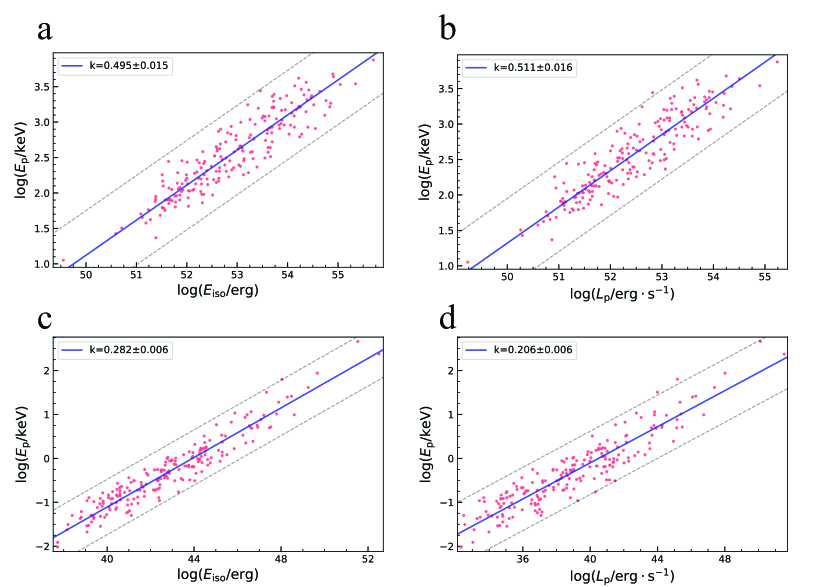
Figure 4: Monte Carlo simulation results. (a,b), Distribution of simulated bursts on the $E_{\rm{p}}-E_{\rm{iso}}$ plane and the $E_{\rm{p}}-L_{\rm{p}}$ plane for the on-axis cases. (c,d), Distribution of simulated bursts on the $E_{\rm{p}}-E_{\rm{iso}}$ plane and the $E_{\rm{p}}-L_{\rm{p}}$ plane for off-axis cases. The solid lines show the best-fitting results for the simulated data points, and the dashed lines represent the $3\sigma$ confidence level. To conclude, for on-axis bursts, the best-fit Amati relation is $E_{\rm{p}}\propto E_{\rm{iso}}^{0.495\pm 0.015}$ and the best-fit Yonetoku relation is $E_{\rm{p}}\propto L_{\rm{p}}^{0.511\pm 0.016}$. For off-axis bursts, the best-fit Amati relation is $E_{\rm{p}}\propto E_{\rm{iso}}^{0.282\pm 0.006}$, while the best-fit Yonetoku relation is $E_{\rm{p}}\propto L_{\rm{p}}^{0.206\pm 0.006}$.

In the off-axis cases, the best-fit slope is $0.282\pm 0.006$ for the $E_{\rm{p}}-E_{\rm{iso}}$ correlation, which is consistent with our expected range of $1/4\sim 4/13$ for the off-axis Amati relation. Similarly, on the $E_{\rm{p}}-L_{\rm{p}}$ plane, the best-fit slope is $0.206\pm 0.006$, which also agrees well with our theoretical range of $1/6\sim 4/17$ for the off-axis Yonetoku relation. Another interesting point in Figure 4c and 4d is that most of the simulated off-axis GRBs have an $E_{\rm{iso}}$ lower than $10^{48}$ erg and an $L_{\rm{p}}$ lower than $10^{46}$ erg s^-1. Only about 5% of our simulated off-axis GRBs have greater $E_{\rm{iso}}$ and $L_{\rm{p}}$. We thus argue that off-axis GRBs are usually LLGRBs. It also indicates that the majority of currently observed normal GRBs should be on-axis GRBs. In Figure 5, all the simulated on-axis and off-axis bursts are plotted in the same panel. Only a very small number of off-axis events are strong enough to be detected. Their distribution obviously deviates from that of the on-axis events on both the $E_{\rm{p}}-E_{\rm{iso}}$ and $E_{\rm{p}}-L_{\rm{p}}$ plane.

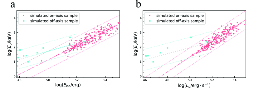
Figure 5: Distribution of simulated off-axis bursts as compared with that of on-axis ones. a, All mock bursts on the $E_{\rm{p}}-E_{\rm{iso}}$ plane. b, All mock bursts on the $E_{\rm{p}}-L_{\rm{p}}$ plane. The dash-dotted line and the dotted line correspond to the best-fit result for on- and off-axis samples, respectively. The dashed lines represent the corresponding $3\sigma$ confidence level. Most of the off-axis bursts are too weak to appear in the two panels here.

Using the mock bursts, we can also test the Ghirlanda relation (Ghirlanda et al., 2004), which links $E_{\rm{p}}$ with the collimation-corrected energy of $E_{\gamma}=(1-\cos\theta_{\rm{jet}})E_{\rm{iso}}$. The distribution of the simulated bursts on the $E_{\rm{p}}-E_{\gamma}$ plane is shown in Figure 6. The data points are best fit by a power-law function of $E_{\rm{p}}\propto E_{\gamma}^{0.459\pm 0.018}$ for the on-axis case (Figure 6a), with an intrinsic scatter of $0.263\pm 0.031$. This agrees well with the recently updated Ghirlanda relation of $E_{\rm{p}}\propto E_{\gamma}^{0.44\pm 0.07}$ for a sample of 55 observed GRBs (Wang et al., 2018). For the off-axis case (Figure 6b), we find $E_{\rm{p}}\propto E_{\gamma}^{0.269\pm 0.008}$, with a larger scatter of $0.272\pm 0.029$. This indicates that the Ghirlanda relation may be largely connected with the Amati relation, but compared with the latter, the slope of the Ghirlanda relation is slightly flatter, and the data points are also obviously more scattered. It is difficult task to compare the off-axis Ghirlanda relation with observations because it needs the precise determination of both the beaming angle and the viewing angle for a number of off-axis GRBs, which themselves are rather dim.

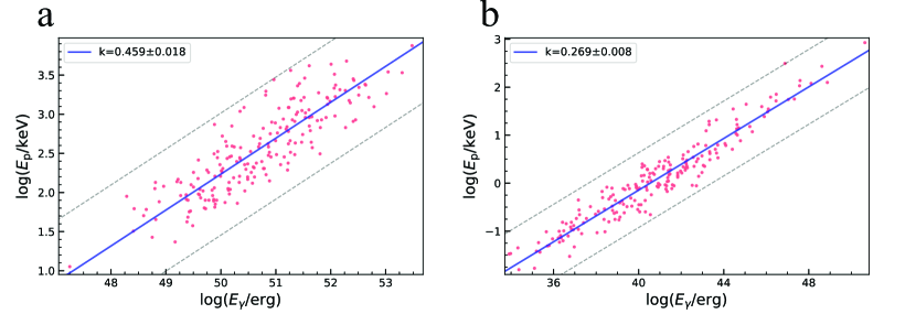
Figure 6: Distribution of the mock GRBs on the $E_{\rm{p}}-E_{\gamma}$ plane for the on-axis case. Panel a On-axis case. Panel b Off-axis case. The solid line shows the best-fit result for the simulated data points, and the dashed lines represent the $3\sigma$ confidence level. The on-axis Ghirlanda relation is $E_{\rm{p}}\propto E_{\gamma}^{0.459\pm 0.018}$, and the off-axis Ghirlanda relation reads $E_{\rm{p}}\propto E_{\gamma}^{0.269\pm 0.008}$.

6 Comparison with observations

In Section 5 we illustrated the simulated $E_{\rm{p}}-E_{\rm{iso}}$ and $E_{\rm{p}}-L_{\rm{p}}$ relations for both on-axis and off-axis cases. We now proceed to compare our results with observational data.

A sample containing 172 long GRBs was used for this purpose, 162 of which were collected from the previous study by Demianski et al. (2017) and Nava et al. (2012). $E_{\rm{p}}$ and $E_{\rm{iso}}$ parameters are available for all these 162 events. The $L_{\rm{p}}$ parameter is available for only 45 GRBs (Nava et al., 2012). Additionally, we collected another 10 bursts that were argued to be possible outliers of the normal Amati relation in previous studies. It has been suggested that they might be off-axis GRBs (Yamazaki et al., 2003b; Ramirez-Ruiz et al., 2005). The observational data of these 10 events are listed in Table 2.

All the observed GRB samples are plotted on the $E_{\rm{p}}-E_{\rm{iso}}$ and $E_{\rm{p}}-L_{\rm{p}}$ planes in Figure 7. Most of the GRBs are well consistent with our on-axis results, thus they both follow the Amati relation and the Yonetoku relation.

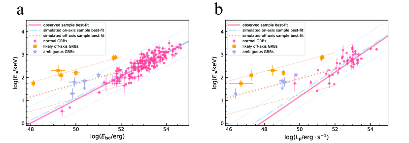
Figure 7: Distribution of all the observed GRBs. Panel a $E_{\rm{p}}$ vs. $E_{\rm{iso}}$. Panel b $E_{\rm{p}}$ vs. $L_{\rm{p}}$. The dash-dotted lines represent our theoretical results for on-axis bursts, and the thick dotted line shows our theoretical results for off-axis bursts. The $3\sigma$ confidence levels are marked correspondingly. The solid lines are the best-fit results for normal GRBs.

On the $E_{\rm{p}}-E_{\rm{iso}}$ plane (Figure 7a), four of the ten possible outliers are located between our on- and off-axis lines. It is thus difficult to judge whether these events are on-axis or off-axis GRBs simply from the Amati relation. However, the remaining six bursts can only be matched by our off-axis line. They should indeed be off-axis events. Figure 4c and 4d clearly show that most off-axis GRBs should be LLGRBs with $E_{\rm{iso}}<10^{48}$ erg, with only a small portion falling in the range of $10^{48}-10^{52}$ erg (see also Figure 5a). This is easy to understand. The input parameters should take some extreme values for an off-axis GRB to be strong enough. Especially these off-axis events should generally have a low $\theta_{\rm{obs}}-\theta_{\rm{jet}}$ value (see Equation 27), which means that they are still slightly off-axis. In Figure 7a, only a small number of GRBs are outliers of the on-axis Amati relation. This low event rate is also consistent with our simulation results.

For the $E_{\rm{p}}-L_{\rm{p}}$ correlation (Figure 7b), we note that almost all the ten possible outliers clearly deviate from the on-axis Yonetoku relation. From combining the Amati relation and the Yonetoku relation, we therefore argue that the ambiguous sample should also be off-axis GRBs. Furthermore, Figure 7 seems to indicate that the Yonetoku relation may be a better tool for distinguishing between on- and off-axis GRBs.

7 Conclusions and discussion

The prompt emission of GRBs was studied for both on- and off-axis cases. Especially the three prompt emission parameters $E_{\rm{p}}$, $E_{\rm{iso}}$, and $L_{\rm{p}}$ were considered. Their dependence on the input model parameters was obtained via both analytical derivations and numerical simulations, which are consistent with each other. We confirmed that $E_{\rm{p}}$, $E_{\rm{iso}}$, and $L_{\rm{p}}$ are independent of $\theta_{\rm{obs}}$ and $\theta_{\rm{jet}}$ as long as our line of sight is within the homogeneous jet cone (i.e., the on-axis cases). However, they strongly depend on the value of $\theta_{\rm{obs}}-\theta_{\rm{jet}}$ when the jet is viewed off-axis. Additionally, their dependence on $\gamma$ is very different for on- and off-axis cases, as shown in Equations 26 and 27. Through Monte Carlo simulations, we found that the Amati relation is $E_{\rm{p}}\propto E_{\rm{iso}}^{0.495\pm 0.015}$ in on-axis cases. Correspondingly, the Yonetoku relation is $E_{\rm{p}}\propto L_{\rm{p}}^{0.511\pm 0.016}$. On the other hand, in off-axis cases, the Amati relation is $E_{\rm{p}}\propto E_{\rm{iso}}^{0.282\pm 0.006}$ and the Yonetoku relation is $E_{\rm{p}}\propto L_{\rm{p}}^{0.206\pm 0.006}$. The simulated samples were directly compared with the observational samples. We found that they are well consistent with each other in the slopes and intrinsic scatters. The $E_{\rm{p}}-E_{\gamma}$ relation was also tested and was found to be $E_{\rm{p}}\propto E_{\gamma}^{0.459\pm 0.018}$ for on-axis GRBs and $E_{\rm{p}}\propto E_{\gamma}^{0.269\pm 0.008}$ for off-axis GRBs.

We have focused on the empirical correlations of long GRBs in the above analysis. Here we present some discussion of short GRBs. Generally speaking, long GRBs usually contain many pulses (tens or even up to hundreds) in their light curves, while short GRBs contain much fewer pulses. For short GRBs, we can therefore perform a similar analysis, but only when the number of pulses considered is reduced significantly. In our model, the total energy release ($E_{\rm{iso}}$) is proportional to the number of pulses, while the peak luminosity ($L_{\rm{p}}$) and the spectral parameter $E_{\rm{p}}$ are nearly irrelevant. In other words, a short GRB will have a much smaller $E_{\rm{iso}}$, but its $L_{\rm{p}}$ and $E_{\rm{p}}$ are largely unchanged. As a result, short GRBs will follow a parallel track on the $E_{\rm{p}}-E_{\rm{iso}}$ plane as compared with long GRBs, the only difference is that their $E_{\rm{iso}}$ are significantly smaller. Alternatively speaking, the power-law index of the Amati relation should be the same for short GRBs and long GRBs, consistent with currently available observations (Zhang et al., 2009, 2018). As for the Yonetoku relation on the $E_{\rm{p}}-L_{\rm{p}}$ plane, we argue that it should be almost identical for both long and short GRBs. However, the number of currently available short GRBs that is suitable for exploring the Yonetoku relation (i.e., for which $E_{\rm{p}}$ and $L_{\rm{p}}$ are measured) in detail is still too small.

A simple top-hat jet geometry was adopted in this study. It should be noted that the GRB outflow might be a structured jet (Ioka & Nakamura, 2018). A recent study suggested that $E_{\rm{p}}$ and the flux will not change much, regardless of the choice of a top-hat jet or a not-too-complicated structured jet (Farinelli et al., 2021). However, in some more complicated scenarios, structured jets may further have an angle-dependent energy density (Lamb et al., 2021). They may be choked jets or even in jet-cocoon systems (Ioka & Nakamura, 2018; Mooley et al., 2018; Troja et al., 2019). The empirical correlations of GRBs in these situations are beyond the scope of this study and could be further considered in the future.

In our calculations, the prompt emission was assumed to be due to nonthermal radiation from internal shocks. Other mechanisms such as photosphere radiation and magnetic reconnection above the photosphere may also contribute to the observed flux of GRBs. Generally, there are two types of photosphere models: nondissipative photosphere models, and dissipative photosphere models. The former can produce a narrow quasi-Planckian component and could account for the thermal component observed in some GRBs (Pe’er, 2008; Beloborodov, 2011), although this component does not play a dominant role in most GRBs (Guiriec et al., 2011; Axelsson et al., 2012). In the dissipative photosphere models, various subphotosphere dissipation processes (Rees & Mészáros, 2005), especially Comptonization, may affect the spectrum (Thompson, 1994; Pe’er et al., 2006; Pe’er & Ryde, 2011; Veres & Mészáros, 2012), which may lead to a nonthermal spectrum. Some authors have even used this model to explain the Band spectrum of GRBs (Thompson, 1994; Beloborodov, 2013; Lundman et al., 2013). Reconnection above the photosphere has also been considered, especially in the view of the ICMART model, focusing on Poynting-flux-dominated outflows (Zhang & Yan, 2011; Zhang & Zhang, 2014). It is still unclear how commonly photosphere radiation and magnetic reconnection are involved in the prompt phase of GRBs. If these radiation mechanisms are included, the derivation will become much more complicated, but it deserves a trial in the future.

The Amati and Yonetoku relations are essential for us to understand the nature of GRBs. They can also help us probe the high-redshift universe (Xu et al., 2021; Hu et al., 2021; Zhao & Xia, 2022; Jia et al., 2022; Deng et al., 2023). Our study shows that they are due to the ultra-relativistic effect of highly collimated jets. To be more specific, they mainly result from the variation in the Lorentz factor in different events. It may provide useful insights for a better understanding of these empirical correlations.

Table 2: Some possible outliers

Likely off-axis sample
GRB Name	z	$\log(E_{\rm{p}})$	$\log(E_{\rm{iso}})$	$\log(L_{\rm{p}})$	Refs
(Units)		(keV)	($10^{52}$ erg)	($10^{51}$ erg s-1)
GRB 980425	0.0085	1.74$\pm$0.16	-3.89$\pm$0.07	-4.32$\pm$0.69	2, 7
GRB 031203	0.106	2.2$\pm$0.14	-2$\pm$0.17	-1.92$\pm$0.09	1, 2
GRB 061021	0.346	2.85$\pm$0.15	-0.34$\pm$0.08	0.24$\pm$0.11	4, 11
GRB 080517	0.09	2.3$\pm$0.23	-2.79$\pm$0.32	-2.52$\pm$0.25	3, 5
GRB 140606B	0.384	2.88$\pm$0.1	-0.24$\pm$0.02	0.3$\pm$0.02	10
GRB 171205	0.0368	2.1$\pm$0.24	-2.66$\pm$0.11	-3.74$\pm$0.09	10, 12
Ambiguous sample
GRB Name	z	$\log(E_{\rm{p}})$	$\log(E_{\rm{iso}})$	$\log(L_{\rm{p}})$	Refs
(Units)		(keV)	($10^{52}$ erg)	($10^{51}$ erg s-1)
GRB 100316D	0.059	1.3$\pm$0.22	-2.16$\pm$0.11	-4.62$\pm$0.01	7, This work
GRB 120422A	0.28253	$<$1.86	-1.62$\pm$0.14	-1.99$\pm$0.18	8, 6
GRB 150818	0.282	2.11$\pm$0.1	-1$\pm$0.09	-1.21$\pm$0.06	8, This work
GRB 161219B	0.1475	1.8$\pm$0.21	-2.07$\pm$0.26	-1.85$\pm$0.31	9