Two-dimensional coherent spectroscopy of trion-polaritons and exciton-polaritons in atomically thin transition metal dichalcogenides

Abstract

We present a microscopic many-body calculation of the nonlinear two-dimensional coherent spectroscopy (2DCS) of trion-polaritons and exciton-polaritons in charge-tunable transition-metal-dichalcogenides monolayers placed in an optical microcavity. The charge tunability leads to an electron gas with nonzero density that brings brightness to the trion - a polaron quasiparticle formed by an exciton with a nonzero residue bounded to the electron gas. As a result, a trion-polariton is created under strong light-matter coupling, as observed in the recent experiment by Sidler et al. [Nat. Phys. 13, 255 (2017)]. We analyze in detail the structure of trion-polaritons, by solving an extended Chevy ansatz for the trion quasiparticle wave-function. We confirm that the effective light-matter coupling for trion-polaritons is determined by the residue of the trion quasiparticle. The solution of the full many-body polaron states within Chevy ansatz enables us to microscopically calculate the nonlinear 2DCS spectrum of both trion-polaritons and exciton-polaritons. We predict the existence of three kinds of off-diagonal cross-peaks in the 2DCS spectrum, as an indication of the coherence among the different branches of trion-polaritons and exciton-polaritons. Due to the sensitivity of 2DCS spectrum to quasiparticle interactions, our work provides a good starting point to explore the strong nonlinearity exhibited by trion-polaritons in some recent exciton-polariton experiments.

I Introduction

Exciton-polaritons in microcavities are hybrid light-matter quasiparticles, formed due to strong coupling between excitons and tightly confined optical modes Deng2010 ; Carusotto2013 ; Byrnes2014 . Owing to the half-matter, half-light nature, they open a research frontier of polaritonics to explore novel nonlinear quantum phenomena that are impossible to observe in linear optical systems and are difficult to reach in pure matter systems. This potential is further amplified by the recent manipulation of atomically thin transition metal dichalcogenides (TMD) Novoselov2005 ; Wang2018 ; Berkelbach2018 , such as MoS₂, WS₂, MoSe₂, and WSe₂. In these two-dimensional materials, robust bright excitons of electrons and holes with relatively large effective masses and large exciton binding energy dominate the optical response even at room temperature. As a result, TMD monolayers are promising candidates for ultrafast polariton-based nonlinear optical integrated devices, such as ultra-low threshold lasers, fast and low-power switches, and all-optical integrated quantum gates. For this purpose, strong polariton nonlinearity is typically required. However, so far it remains a challenge to obtain strong exciton-exciton interaction and polariton-polariton interaction Hu2020 .

In this respect, the recent observation of trion-polaritons in charge-tunable MoSe₂ monolayers by Sidler et al. received considerable interest Sidler2017 . At first glance, the existence of trion-polaritons is a surprise, since a trion is a fermionic three-particle bound-state of one hole and two electrons and therefore in principle it should not be able to couple with bosonic photon of light. But now, we understand that trions in charge-tunable monolayers are actually the quasiparticles of Fermi polarons Efimkin2017 , which are excitons (as impurities) dressed by the whole Fermi sea of an electron gas Massignan2014 ; Schmidt2018 ; Wang2022PRL ; Wang2022PRA . Except in the true trion limit (with vanishing electron gas density), where the three-particle bound-state is recovered, the trion is better viewed as a dressed exciton with a nonzero residue that characterizes the free motion of the exciton Sidler2017 ; Efimkin2017 . As a result, cavity mode can indeed couple to the trion and lead to the formation of trion-polaritons. The real surprise of trion-polaritons comes with the observation that there seems to be a large nonlinearity in the optical response, as revealed by the pump-probe measurement Tan2020 . The understanding of such a large nonlinearity has been the focus of several theoretical analyses Rana2021 ; BastarracheaMagnani2021 ; Song2022arXiv . Further experimental investigations are definitely needed. In particular, a nonlinear four-wave-mixing measurement, such as the two-dimensional coherent spectroscopy (2DCS) Jonas2003 ; Li2006 ; Cho2008 ; Hao2016NanoLett ; Muir2022 would be ideally suitable to quantitatively characterize the large nonlinearity of trion-polaritons.

The purpose of this work is two-fold. On the one hand, we wish to clarify the nature of trion-polaritons by carefully examining the full many-body Fermi polaron wave-functions of either exciton-polariton or trion-polariton, with the use of the Chevy ansatz that describes the one-particle-hole excitations of the Fermi sea Chevy2006 . The variational Chevy ansatz Chevy2006 (or equivalently the many-body $T$-matrix theory Hu2022 ) has been previously used to determine the self-energy and the spectral function of trion-polaritons Sidler2017 ; BastarracheaMagnani2021 . However, a detail analysis of the many-body wave-functions is of lack. Here, our strategy is to follow the recent theoretical study of the wave-functions of the three-particle trion bound state Zhumagulov2022 ; Tempelaar2019 , where a single excess electron is approximately used to simulate the whole Fermi sea through the $k$-space discretization. Our calculation is free from such a $k$-space approximation. A trade-off, however, is the ignorance of the internal degree of freedom of the exciton wave-function. This ignorance is fully justified by the large exciton binding energy ($\sim 500$ meV), which is at least ten times larger than the trion binding energy in TMD monolayers ($\sim 30$ meV) Wang2018 . The internal structure of excitons then should only bring negligible effects on the low-energy properties of trion-polaritons.

On the other hand, the full many-body Fermi polaron wave-functions obtained within the Chevy ansatz approximation allow us to microscopically calculate the 2DCS spectrum of trion-polaritons, in addition to that of exciton-polaritons. The microscopic determination of the 2DCS spectrum of an interacting many-body system is highly non-trivial Lindoy2022 ; Wang2022arXiv1 ; Wang2022arXiv2 ; Hu2022arXiv . Therefore, we would like to restrict ourselves to the case of a single trion-polariton or exciton-polariton in the system Hu2022arXiv . This rules out the possibility of addressing the interaction effect between two trion-polaritons that is of major interest. However, our calculation would capture the basic features of the 2DCS spectrum, which could then be used to discriminate the possible interaction effects between two trion-polaritons in future 2DCS measurements.

The rest of the paper is organized as follows. In the next section (Sec. II), we outline the model Hamiltonian for the Fermi-polaron-polaritons in TMD monolayers and present the many-body solutions by using the Chevy ansatz approximation. In Sec. III, we discuss the structures of trion-polaritons and exciton-polaritons and the optical responses of both photons and excitons. In Sec. IV, we predict the the 2DCS spectroscopy and discuss in detail the off-diagonal cross-peaks, which show the coherence between exciton-polaritons and trion-polaritons. Finally, Sec. V is devoted to conclusions and outlooks.

II Model Hamiltonian and the Chevy ansatz solution

In charge-tunable TMD monolayers, tightly bound excitons formed by electrons and holes near the $K$ (or $K^{\prime}$) valley move in the Fermi sea of an electron gas in other valley with a nonzero electron density that corresponds to a Fermi energy at about $\varepsilon_{F}\sim 10$ meV. Electrons in the electron gas have opposite spin with respect to the electron inside excitons. Therefore, their effective interaction with excitons is attractive and is well characterized by a contact interaction with strength $U<0$, whose magnitude is tuned to yield the trion binding energy $E_{T}\sim 30$ meV Tempelaar2019 . The TMD monolayers can be placed in the antinode of a planar photonic microcavity, with cavity photon mode being tuned near resonance with the excitonic and trionic optical transitions.

II.1 Model Hamiltonian

We denote the cavity photon mode and the exciton by the creation (or annihilation) field operators $a_{\mathbf{k}}^{\dagger}$ ($a_{\mathbf{k}}$) and $X_{\mathbf{k}}^{\dagger}$ ($X_{\mathbf{k}}$), respectively. The electrons in the electron gas are described by the creation and annihilation field operators $c_{\mathbf{k}}^{\dagger}$ and $c_{\mathbf{k}}$. The polariton system under consideration therefore can be well described by a Fermi polaron model Hamiltonian ($\hbar=1$) Sidler2017 ,

$$\mathcal{H} = \mathcal{H}_{aX}^{(0)}+\sum_{\mathbf{k}}\epsilon_{\mathbf{k}}c_{\mathbf{k}}^{\dagger}c_{\mathbf{k}}+U\sum_{\mathbf{qkp}}X_{\mathbf{k}}^{\dagger}c_{\mathbf{q-k}}^{\dagger}c_{\mathbf{q}-\mathbf{p}}X_{\mathbf{p}},$$ (1)

$$\mathcal{H}_{aX}^{(0)} = \sum_{\mathbf{k}}\left[\omega_{\mathbf{k}}a_{\mathbf{k}}^{\dagger}a_{\mathbf{k}}+\epsilon_{\mathbf{k}}^{X}X_{\mathbf{k}}^{\dagger}X_{\mathbf{k}}+\frac{\Omega}{2}\left(a_{\mathbf{k}}^{\dagger}X_{\mathbf{k}}+h.c.\right)\right].$$ (2)

Here, $\epsilon_{\mathbf{k}}=k^{2}/(2m_{e})$, $\omega_{\mathbf{k}}=k^{2}/(2m_{\textrm{ph}})+\delta$ and $\epsilon_{\mathbf{k}}^{X}=k^{2}/(2m_{X})$ are the single-particle energy dispersion relation of electrons, cavity photons and excitons, respectively, with electron mass $m_{e}$, photon mass $m_{\textrm{ph}}\sim 10^{-5}m_{e}$ and exciton mass $m_{X}\simeq 2m_{e}$ in 2D TMD materials Wang2018 ; $\delta$ is the photon detuning measured in relative to the exciton energy level; and finally, $\Omega$ is the light-matter coupling (i.e., Rabi coupling). We will restrict ourselves to the case that the maximum number of exciton-polaritons is one, i.e.,

$$\sum_{\mathbf{k}}(a_{\mathbf{k}}^{\dagger}a_{\mathbf{k}}+X_{\mathbf{k}}^{\dagger}X_{\mathbf{k}})\leq 1,$$ (3)

which realizes the Fermi polaron limit. In contrast, the density of the electrons ($n=\sum_{\mathbf{k}}c_{\mathbf{k}}^{\dagger}c_{\mathbf{k}}$) is tunable, by adjusting the Fermi energy $\varepsilon_{F}$ through gate voltage in the experiments Sidler2017 ; Tan2020 .

In the absence of the electron gas, the strong light-matter coupling leads to the well-defined two branches of exciton-polaritons: the lower polariton and upper polariton Deng2010 ; Carusotto2013 ; Byrnes2014 . With the electron gas, one may naively anticipate the effective interactions between lower (upper) polarities and the electron gas, and hence the formation of two separate lower and upper branches of Fermi polarons. However, the correct physical picture turns out to be the formation of attractive and repulsive Fermi polarons of dressed excitons in the first place, and then the coupling of Fermi polarons to the light. For this reason, the trion-polaritons is better viewed as Fermi-polaron-polaritons Sidler2017 , where the treatment of a trion as an attractive Fermi polaron is explicitly emphasized.

II.2 The Chevy ansatz solution

To solve the model Hamiltonian in the case of one exciton-polariton, let us take the following Chevy ansatz,

$$\left|P\right\rangle = \left(\phi_{0}X_{0}^{\dagger}+\tilde{\phi}_{0}a_{0}^{\dagger}+\sum_{\mathbf{k}_{p}\mathbf{k}_{h}}\phi_{\mathbf{k}_{p}\mathbf{k}_{h}}X_{-\mathbf{k}_{p}+\mathbf{k}_{h}}^{\dagger}c_{\mathbf{k}_{p}}^{\dagger}c_{\mathbf{k}_{h}}\right.$$ (4)

$$\left.+\sum_{\mathbf{k}_{p}\mathbf{k}_{h}}\tilde{\phi}_{\mathbf{k}_{p}\mathbf{k}_{h}}a_{-\mathbf{k}_{p}+\mathbf{k}_{h}}^{\dagger}c_{\mathbf{k}_{p}}^{\dagger}c_{\mathbf{k}_{h}}\right)\left|\textrm{FS}\right\rangle,$$

for the Fermi-polaron-polariton states with zero total momentum $\mathbf{K=0}$. Here, the Fermi sea at zero temperature $\left|\textrm{FS}\right\rangle$ is obtained by filling the single-particle energy level $\epsilon_{\mathbf{k}}$ with $N$ electrons, from the bottom of the energy band up to the energy $\varepsilon_{F}$. The hole momentum $\mathbf{k}_{h}$ and the particle momentum $\mathbf{k}_{p}$ satisfy the constraints $\epsilon_{\mathbf{k}_{h}}\leqslant\varepsilon_{F}$ and $\epsilon_{\mathbf{k}_{p}}>\varepsilon_{F}$, respectively. The energy of the whole Fermi sea is denoted as $E_{\textrm{FS}}$.

The ansatz involves the free motions of excitons and photons with the amplitudes $\phi_{0}$ and $\tilde{\phi}_{0}$, respectively. It also describes the one-particle-hole excitations of the Fermi sea due to the inter-particle interaction of excitons and electrons, with the amplitude $\phi_{\mathbf{k}_{p}\mathbf{k}_{h}}$. Although there is no direct interaction between photons and electrons, for completeness we include the terms $a_{-\mathbf{k}_{p}+\mathbf{k}_{h}}^{\dagger}c_{\mathbf{k}_{p}}^{\dagger}c_{\mathbf{k}_{h}}\left|\textrm{FS}\right\rangle$ with the amplitude $\tilde{\phi}_{\mathbf{k}_{p}\mathbf{k}_{h}}$. These terms actually do not contribute to the ansatz due to the negligible photon mass, since the related energy would be extremely large (i.e., $\omega_{\mathbf{k}}$ becomes very significant for nonzero $\mathbf{k}\neq 0$).

Unlike the previous works that only minimize the ground-state energy of the Chevy ansatz for the variational parameters ($\phi_{0}$, $\tilde{\phi}_{0}$, $\phi_{\mathbf{k}_{p}\mathbf{k}_{h}}$ and $\tilde{\phi}_{\mathbf{k}_{p}\mathbf{k}_{h}}$) or the self-energy of polaritons Sidler2017 ; Tan2020 , here we are interested in solving all the many-body Fermi-polaron-polariton states, by using an alternative exact diagonalization approach. To this aim, we put the system - consisting of $N$ electrons and a single exciton-polariton - onto a two-dimensional square lattice with $L\times L$ sites. The electron density then takes the value

$$n=\frac{N}{(La)^{2}},$$ (5)

where $a$ is the lattice spacing and unless specified otherwise is set to be unity ($a=1$). We consider that the exciton, photon, and electrons hop on the lattice only to the nearest neighbor with strengths $t_{a}$, $t_{X}$ and $t_{c}$, respectively. Their single-particle energy dispersion relations are then given by ($\tilde{\omega}_{\mathbf{k}}=\omega_{\mathbf{k}}-\delta$),

$$\tilde{\omega}_{\mathbf{k}} = -2t_{a}\left[\cos\left(k_{x}\right)+\cos\left(k_{y}\right)\right]+4t_{a}\simeq\frac{k_{x}^{2}+k_{y}^{2}}{2m_{\textrm{ph}}},$$ (6)

$$\epsilon_{\mathbf{k}}^{X} = -2t_{X}\left[\cos\left(k_{x}\right)+\cos\left(k_{y}\right)\right]+4t_{X}\simeq\frac{k_{x}^{2}+k_{y}^{2}}{2m_{X}},$$ (7)

$$\epsilon_{\mathbf{k}} = -2t_{c}\left[\cos\left(k_{x}\right)+\cos\left(k_{y}\right)\right]+4t_{c}\simeq\frac{k_{x}^{2}+k_{y}^{2}}{2m_{e}},$$ (8)

where $m_{\textrm{ph}}\equiv 1/(2t_{a}a^{2})$, $m_{X}\equiv 1/(2t_{X}a^{2})$ and $m_{e}\equiv 1/(2t_{c}a^{2})$ in the dilute limit ($n\rightarrow 0$) that is of interest. In the same limit, we have the relation

$$\varepsilon_{F}\simeq 4\pi nt_{c}=\frac{4\pi N}{L^{2}}t_{c}.$$ (9)

It is also easy to see the relations $t_{a}/t_{c}=m_{e}/m_{\textrm{ph}}\sim 10^{5}$ and $t_{X}/t_{c}=m_{e}/m_{X}\simeq 1/2$. We assume the periodic boundary condition, so the momentum $\mathbf{k}$ on the lattice takes the values,

$$\left(k_{x},k_{y}\right)=\left(\frac{2\pi n_{x}}{L},\frac{2\pi n_{y}}{L}\right),$$ (10)

with the integers $n_{x},n_{y}=-L/2+1,\cdots-1,0,1,\cdots L/2$.

On the square lattice, we may identify that the Hilbert space of the model Hamiltonian involves four different types of expansion basis states (at zero polaron momentum),

$$\left|1\right\rangle = X_{0}^{\dagger}\left|\textrm{FS}\right\rangle,$$ (11)

$$\left|2\right\rangle = a_{0}^{\dagger}\left|\textrm{FS}\right\rangle,$$ (12)

$$\left|3\right\rangle_{\mathbf{k}_{p}\mathbf{k}_{h}} = X_{-\mathbf{k}_{p}+\mathbf{k}_{h}}^{\dagger}c_{\mathbf{k}_{p}}^{\dagger}c_{\mathbf{k}_{h}}\left|\textrm{FS}\right\rangle,$$ (13)

$$\left|4\right\rangle_{\mathbf{k}_{p}\mathbf{k}_{h}} = a_{-\mathbf{k}_{p}+\mathbf{k}_{h}}^{\dagger}c_{\mathbf{k}_{p}}^{\dagger}c_{\mathbf{k}_{h}}\left|\textrm{FS}\right\rangle,$$ (14)

It is straightforward to see that the dimension of the Hilbert space is $D=2+2N(L^{2}-N)$. By using the expansion basis states, the Fermi-polaron-polariton model Hamiltonian then is casted into a $D\times D$ Hermitian matrix, with the following matrix elements ($\mathcal{H}_{ji}=\mathcal{H}_{ij}^{*}$),

$$\left\langle 1\right|\mathcal{H}\left|1\right\rangle = E_{\textrm{FS}}+nU,$$ (15)

$$\left\langle 1\right|\mathcal{H}\left|2\right\rangle = \frac{\Omega}{2},$$ (16)

$$\left\langle 1\right|\mathcal{H}\left|3\right\rangle_{\mathbf{k}^{\prime}_{p}\mathbf{k}^{\prime}_{h}} = \frac{U}{L^{2}},$$ (17)

$$\left\langle 1\right|\mathcal{H}\left|4\right\rangle_{\mathbf{k}^{\prime}_{p}\mathbf{k}^{\prime}_{h}} = 0,$$ (18)

and

$$\left\langle 2\right|\mathcal{H}\left|2\right\rangle = E_{\textrm{FS}}+\delta,$$ (19)

$$\left\langle 1\right|\mathcal{H}\left|3\right\rangle_{\mathbf{k}^{\prime}_{p}\mathbf{k}^{\prime}_{h}} = 0,$$ (20)

$$\left\langle 2\right|\mathcal{H}\left|4\right\rangle_{\mathbf{k}^{\prime}_{p}\mathbf{k}^{\prime}_{h}} = 0,$$ (21)

and

$${}_{\mathbf{k}_{h}\mathbf{k}_{p}}\left\langle 3\right|\mathcal{H}\left|3\right\rangle_{\mathbf{k}^{\prime}_{p}\mathbf{k}^{\prime}_{h}} = \left[E_{\textrm{FS}}+\epsilon_{\mathbf{k}_{p}}-\epsilon_{\mathbf{k}_{h}}+\epsilon_{-\mathbf{k}_{p}+\mathbf{k}_{h}}^{X}+nU\right]\delta_{\mathbf{k}_{p}\mathbf{k}^{\prime}_{p}}\delta_{\mathbf{k}_{h}\mathbf{k}^{\prime}_{h}}+\frac{U}{L^{2}}\left(\delta_{\mathbf{k}_{h}\mathbf{k}^{\prime}_{h}}-\delta_{\mathbf{k}_{p}\mathbf{k}^{\prime}_{p}}\right),$$ (22)

$${}_{\mathbf{k}_{h}\mathbf{k}_{p}}\left\langle 3\right|\mathcal{H}\left|4\right\rangle_{\mathbf{k}^{\prime}_{p}\mathbf{k}^{\prime}_{h}} = \frac{\Omega}{2}\delta_{\mathbf{k}_{p}\mathbf{k}^{\prime}_{p}}\delta_{\mathbf{k}_{h}\mathbf{k}^{\prime}_{h}},$$ (23)

$${}_{\mathbf{k}_{h}\mathbf{k}_{p}}\left\langle 4\right|\mathcal{H}\left|4\right\rangle_{\mathbf{k}^{\prime}_{p}\mathbf{k}^{\prime}_{h}} = \left[E_{\textrm{FS}}+\epsilon_{\mathbf{k}_{p}}-\epsilon_{\mathbf{k}_{h}}+\omega_{-\mathbf{k}_{p}+\mathbf{k}_{h}}\right]\delta_{\mathbf{k}_{p}\mathbf{k}^{\prime}_{p}}\delta_{\mathbf{k}_{h}\mathbf{k}^{\prime}_{h}}.$$ (24)

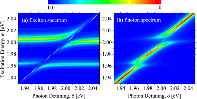
Figure 1: Two-dimensional contour plots of the zero-momentum spectral function of the exciton (a) and of the photon (b), as a function of the photon detuning $\delta$ at the electron Fermi energy $\varepsilon_{F}=7.8$ meV. The two black horizontal dot-dashed lines show the energies of the exciton (i.e., the repulsive polaron branch with $\varepsilon_{X}\simeq 2004.4$ meV) and the trion (i.e., the attractive polaron branch with $\varepsilon_{T}\simeq 1963.5$ meV), in the absence of the cavity photon field. The diagonal white dotted line indicates the cavity photon detuning $\delta$. Two avoided crossings at $\omega=\varepsilon_{X}$ and $\omega=\varepsilon_{T}$ are clearly visible. The spectral functions are measured in arbitrary units and are plotted in a linear scale.

We diagonalize the $D\times D$ Hermitian matrix to obtain all the eigenvalues $E^{(n)}$ and eigenstates, from which we extract the Fermi-polaron-polariton energies $\mathcal{E}^{(n)}=E^{(n)}-E_{\textrm{FS}}$, the residue of excitons $Z_{X}^{(n)}\equiv\phi_{0}^{(n)*}\phi_{0}^{(n)}$ and the residue of photons $Z_{\textrm{ph}}^{(n)}\equiv\tilde{\phi}_{0}^{(n)*}\tilde{\phi}_{0}^{(n)}$. Furthermore, we directly calculate the retarded Green functions of excitons and photons,

$$G_{X}\left(k=0,\omega\right) = \sum_{n}\frac{Z_{X}^{(n)}}{\omega-\mathcal{E}^{(n)}+\omega_{X}+i\delta},$$ (25)

$$G_{\textrm{ph}}\left(k=0,\omega\right) = \sum_{n}\frac{Z_{\textrm{ph}}^{(n)}}{\omega-\mathcal{E}^{(n)}+\omega_{X}+i\delta}.$$ (26)

and the associated spectral functions

$$A_{X}(k=0,\omega) = -\frac{1}{\pi}\textrm{Im}G_{X}(k=0,\omega),$$ (27)

$$A_{\textrm{ph}}(k=0,\omega) = -\frac{1}{\pi}\textrm{Im}G_{\textrm{ph}}(k=0,\omega).$$ (28)

Here, since we use a finite-size square lattice, the level spacing in the single-particle dispersion relation is about $\delta=4t_{c}/L$. We will use $\delta$ to replace the infinitesimal $0^{+}$ in the spectral function and to eliminate the discreteness of the single-particle energy levels. To make connection with the experimental measurement, we measure the energy $\omega$ in the spectral function from the top of the valence band by adding a constant energy shift $\omega_{X}=E_{g}-E_{X}=2$ eV Wang2018 ; Zhumagulov2022 , where $E_{g}$ and $E_{X}$ are the band gap and the binding energy of excitons, respectively.

III Trion polaritons and the one-dimensional optical response

In our numerical calculations, we consider a square lattice of $L=16$. We set the hopping strength $t_{c}=10$ meV and then determine $t_{a}=t_{c}(m_{e}/m_{\textrm{ph}})=10^{6}$ meV and $t_{X}=t_{c}(m_{e}/m_{X})=5$ meV. At these parameters, the spectral broadening factor $\delta=4t_{c}/L=2.5$ meV, which qualitatively agrees the homogeneous broadening observed in the optical response of exciton-polaritons Wang2018 . We take an attractive interaction strength $U=-8t_{c}=-80$ meV, which leads to a trion energy at about $-3.2t_{c}=-32$ meV in the dilute limit (i.e., $n\rightarrow 0$ or $N=1$ at $L=16$), in reasonable agreement with the trion binding energy $E_{T}\sim 30$ meV found in 2D TMD materials Wang2018 .

Most of our calculations are carried out for a number of electrons $N=16$, which corresponds to a Fermi energy $\varepsilon_{F}\simeq 4\pi Nt_{c}/L^{2}\simeq 7.8$ meV Sidler2017 ; Tan2020 . At this number of electrons, we find the attractive polaron energy $E_{A}\simeq-3.65t_{c}=-36.5$ meV and the repulsive polaron energy $E_{R}\simeq+0.44t_{c}=4.4$ meV, without the cavity field. Measured from the top of the valence band, these values give rise to the trion energy $\varepsilon_{T}=E_{A}+\omega_{X}=1963.5$ meV and the exciton energy $\varepsilon_{X}=E_{R}+\omega_{X}=2004.4$ meV.

For convenience, we will also measure the photon detuning $\delta$ with respect to the top of the valence band, and understand it to be $\delta+\omega_{X}$ without any confusion. For the light-matter coupling, we always fix the Rabi frequency to be $\Omega=2t_{c}=20$ meV.

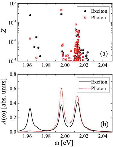
Figure 2: (a) Residues of the exciton (black solid circles) and the photon (red empty square) for each many-body state that is arranged with increasing energy. (b) The spectral function of the exciton (black solid line) and the photon (red dotted line), shown in arbitrary units. Here, we take a cavity photon detuning $\delta=\varepsilon_{X}\simeq 2004.4$ meV. The electron Fermi energy is $\varepsilon_{F}=7.8$ meV.

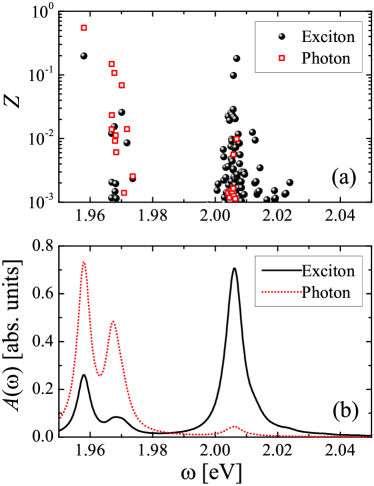
Figure 3: (a) Residues of the exciton (black solid circles) and the photon (red empty square) for each many-body state that is arranged with increasing energy. (b) The spectral function of the exciton (black solid line) and the photon (red dotted line), shown in arbitrary units. Here, we take a photon detuning $\delta=\varepsilon_{T}\simeq 1963.5$ meV. The electron Fermi energy is $\varepsilon_{F}=7.8$ meV.

In Figs. 1(a) and 1(b), we report the zero-momentum spectral functions $A_{X}\left(k=0,\omega\right)$ and $A_{\textrm{ph}}\left(k=0,\omega\right)$ at the typical experimental Fermi energy $\varepsilon_{F}=7.8$ meV for excitons and photons, respectively, in the form of the two-dimensional contour plot with a linear scale (as indicated on the top of the figure). Both spectral functions clearly show an avoided crossing at the energy close to $\omega_{X}=2$ eV. The two branches can be well-understood as the upper and lower polaritons given by the model Hamiltonian $\mathcal{H}_{aX}^{(0)}$, which exist even in the absence of the electron gas. This is evident if we compare Fig. 1 with Fig. 9 in Appendix A, where the latter figure reports the results at a much smaller Fermi energy $\varepsilon_{F}=1$ meV. For the upper and lower polariton branches, we find that the existence of the electron gas will slightly shift the position of the avoided crossing (i.e., from $\omega_{X}=2000$ meV to $\varepsilon_{X}\simeq 2004.4$ meV), due to the exciton-electron interaction that becomes effectively repulsive for the excited state of repulsive polarons.

The main effect of the electron gas to the spectral functions is the appearance of an additional avoided crossing, the trion-polariton, at the trion energy $\omega=\varepsilon_{T}$. At the Fermi energy $\varepsilon_{F}=7.8$ meV in Fig. 1, this avoided crossing has an energy splitting smaller than but comparable to the Rabi coupling $\Omega=20$ meV for the exciton-polariton. The shape of the avoided crossing is apparently asymmetric in the exciton spectrum. At the much smaller Fermi energy $\varepsilon_{F}=1$ meV in Fig. 9, the avoided crossing can hardly be identified in both exciton spectrum and photon spectrum, which unambiguously indicates that the existence of a Fermi sea is the key source for the trion-polariton.

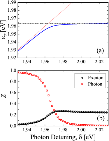
Figure 4: (a) The ground-state energy of Fermi-polaron-polaritons as a function of the photon detuning. The red dotted line and the black dot-dashed line show the cavity photon detuning and the trion energy without cavity field $\varepsilon_{T}\simeq 1963.5$ meV. (b) Residues of the exciton (black solid circles) and the photon (red empty squares) of the ground-state as a function of the photon detuning. Here, we take the electron Fermi energy $\varepsilon_{F}=7.8$ meV.

To better understand the two avoided crossings for exciton-polaritons and trion-polaritons, we show in Fig. 2 and Fig. 3 the residues (upper panel) and spectral functions (lower panel) of excitons and photons, at the photon detuning $\delta=\varepsilon_{X}$ and $\delta=\varepsilon_{T}$, respectively.

Let us first focus on the avoided crossing for exciton-polaritons at $\delta=\varepsilon_{X}\simeq 2004.4$ meV in Fig. 2. The composition of the different branches might be seen from the exciton and photon residues. The upper branch (or the rightest branch) locates at the energy $\sim 2.013$ eV and consists of a number of many-body energy levels that distribute nearby with notable exciton and photon residues. For this upper branch, due to its collective nature, it seems difficult to find a Hopfield coefficient that clearly defines the contributions or components from cavity photons and excitons, as in the case of conventional exciton-polaritons. In contrast, for the lower branch (or the middle branch in the range of the whole plot, which is referred to as middle polariton in the literature) located at the energy $\sim 1.996$ eV, we find that it is only contributed by one dominated state. All other nearby many-body states have residues much less than $1\%$. This branch seems to decouple from the particle-hole excitations of the Fermi sea and therefore retains the characteristic of the exciton-polariton without the electron gas. We note that, the energy splitting between the upper and lower branches is given by $2.013-1.996=0.017$ eV or 17 meV, which is slightly smaller than the Rabi coupling $\Omega=20$ meV. We attribute this slight difference to the transfer of the residue or the oscillator strength to the third branch (the lowest-energy branch) in the exciton spectrum, as shown in Fig. 2(b).

The situation for the avoided crossing of trion-polaritons at $\delta=\varepsilon_{T}$ is very similar. As can be seen from Fig. 3, the upper branch of this avoided crossing near the energy $\sim 1.967$ eV is formed by a bundle of many-body states with significant residues. The lower branch is instead contributed by one state only at the energy $\sim 1.958$ eV. The energy splitting of the two branches is about $9$ meV and is less than the Rabi coupling $\Omega=20$ meV. The small energy splitting is again attributed to the reduced oscillator strength, which we now turn to discuss in greater detail.

As we mentioned earlier, a plausible picture for the formation of trion-polaritons is the strong effective light-matter coupling between a photons and an attractive Fermi polaron of the exciton impurity. It is clear that only the free part of the attractive polaron (as characterized by $\phi_{0}$) contribute to the light-matter coupling, in the form of the term $(\Omega/2)[a_{0}^{\dagger}(\phi_{0}X_{0})+h.c.]$ at zero momentum. In other words, the effective Rabi coupling would be given by

$$\Omega_{\textrm{eff}}\simeq\Omega\phi_{0}=\Omega\sqrt{Z_{X}},$$ (29)

which is reduced by the square root of the excitonic residue. This expression of the effective Rabi coupling would also work well for the repulsive polaron (i.e., the exciton-polariton with the electron gas).

In Fig. 4, we show the ground-state energy of the trion-polariton (a) and its excitonic and photonic residues (b), as a function of the photon detuning $\delta$. The excitonic residue does not change significant when $\delta\geqslant\varepsilon_{X}$. In particular, at the avoided crossing of $\delta=\varepsilon_{X}$, the excitonic residue $Z_{X}\sim 0.25$, which implies an effective Rabi coupling $\Omega_{\textrm{eff}}\simeq\Omega\sqrt{Z_{X}}=10$ meV, which is very close to the observed value of $9$ meV. The slightly reduced Rabi coupling of $17$ meV at the avoided crossing of the exciton-polariton might be understand in a similar way. We may identify that the excitonic residue of the repulsive polaron at $\delta=\varepsilon_{X}$ is about $Z_{X}\sim 0.7$. Therefore the effective Rabi coupling is given by $\Omega_{\textrm{eff}}\simeq\Omega\sqrt{Z_{X}}=16.7$ meV, in agreement with our finding.

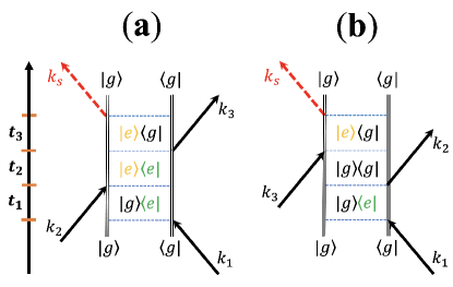
Figure 5: Two double-sided Feynman diagrams that represent the two contributions to the standard rephasing 2D coherent spectra under the phase-match condition $\mathbf{k}_{s}=-\mathbf{k}_{1}+\mathbf{k}_{2}+\mathbf{k}_{3}$, with the time ordering of excitation pulses indicated on the left. The evolution, mixing, and emission time delays are labeled as $t_{1}$, $t_{2}$, and $t_{3}$, respectively. (a) shows the process of excited-state emission (ESE), $R_{2}(t_{1},t_{2},t_{3})$. (c) corresponds to the ground-state bleaching (GSB), $R_{3}(t_{1},t_{2},t_{3})$. In the diagrams, we use $\left|g\right\rangle$ to denote the Fermi sea and $\left|e\right\rangle$ to label the many-body states with an exciton-polariton, respectively. There are infinitely many many-body (Fermi polaron) states $\left|e\right\rangle$, as indicated by different colors.

IV two-dimensional coherent spectroscopy

Let us now consider the 2DCS spectroscopy, which is to be implemented in future experiments on studying the exciton-polariton physics in TMD materials. In 2DCS, three excitation pulses with momentum $\mathbf{k}_{1}$, $\mathbf{k}_{2}$ and $\mathbf{k}_{3}$ are applied to the system under study at times $\tau_{1}$, $\tau_{2}$ and $\tau_{3}$, separated by an evolution time delay $t_{1}=\tau{}_{2}-\tau_{1}$ and a mixing time delay $t_{2}=\tau_{3}-\tau_{2}$, as illustrated in the left part of Fig. 5. These pulses generate a signal with momentum $\mathbf{k}_{s}$, as a result of the nonlinear third-order process of four-wave-mixing. The signal can then be measured after an emission time delay $t_{3}$ by using the frequency-domain heterodyne detection.

During the excitation period, each excitation pulse creates or annihilates an exciton. As the photon momentum of the excitation pulses is negligible, the exciton has the zero momentum. Therefore, each pulse can be described by the interaction operator $V$,

$$V\propto X_{0}+X_{0}^{\dagger}.$$ (30)

Following the standard nonlinear response theory Cho2008 , the four-wave-mixing signal is given by the third-order nonlinear response function,

$$\mathcal{R}^{(3)}\propto\left\langle\left[\left[\left[V\left(t_{1}+t_{2}+t_{3}\right),V\left(t_{1}+t_{2}\right)\right],V\left(t_{1}\right)\right],V\right]\right\rangle,$$ (31)

where the time-dependent interaction operator $V(t)\equiv e^{i\mathcal{H}t}Ve^{-i\mathcal{H}t}$, and $\left\langle\cdots\right\rangle$ stands for the quantum average over the initial many-body configuration of the system without excitation pulses, which at zero temperature is given by the ground state. By expanding the three bosonic commutators, we find four distinct correlation functions and their complex conjugates Cho2008 . For the rephasing mode that is of major experimental interest, $t_{1}>0$ and $\mathbf{k}_{s}=-\mathbf{k}_{1}+\mathbf{k}_{2}+\mathbf{k}_{3}$. For this case, only two contributions are relevant if we consider at most one excitonic excitation in the system: the process of so-called excited-state emission (ESE) Cho2008 ; Hao2016NanoLett ,

$$R_{2}=\left\langle VV\left(t_{1}+t_{2}\right)V\left(t_{1}+t_{2}+t_{3}\right)V\left(t_{1}\right)\right\rangle,$$ (32)

and the process of ground-state bleaching (GSB) Cho2008 ; Hao2016NanoLett ,

$$R_{3}=\left\langle VV\left(t_{1}\right)V\left(t_{1}+t_{2}+t_{3}\right)V\left(t_{1}+t_{2}\right)\right\rangle.$$ (33)

These two processes can be visualized by using double-sided Feynman diagrams, as given in Fig. 5(a) and Fig. 5(b), respectively.

For an exciton system, a microscopic calculation of the 2DCS spectrum has been recently carried out Hu2022arXiv . Here, we extend such a microscopic calculation to the exciton-polariton system. After some straightforward algebra following the line of Ref. Hu2022arXiv , we obtain the ESE and GSB contributions,

$$R_{2} = \sum_{nm}Z_{X}^{(n)}Z_{X}^{(m)}e^{i\mathcal{E}^{(n)}t_{1}}e^{i\left[\mathcal{E}^{(n)}-\mathcal{E}^{(m)}\right]t_{2}}e^{-i\mathcal{E}^{(m)}t_{3}},$$ (34)

$$R_{3} = \sum_{nm}Z_{X}^{(n)}Z_{X}^{(m)}e^{i\mathcal{E}^{(n)}t_{1}}e^{-i\mathcal{E}^{(m)}t_{3}},$$ (35)

where the indices $n$ and $m$ run over the whole many-body polaron states.

These two expressions can be easily understood from the double-sided Feynman diagrams. For the ESE process illustrated in Fig. 5(b), the weight $Z_{X}^{(n)}Z_{X}^{(m)}$ measures the transfer rates between different many-body states induced by the three excitation pulses and the four-wave-mixing signal. For example, the transfer of the first pulse at momentum $\mathbf{k}_{1}$ brings a factor of $\phi_{0}^{(n)}$, while the transfer of the second pulse at momentum $\mathbf{k}_{2}$ comes with a factor of $[\phi_{0}^{(m)}]^{*}$, and so on. When we combine all the four factors for the four transitions, we obtain the weight $Z_{X}^{(n)}Z_{X}^{(m)}$. On the other hand, the three dynamical (time-evolution) phase factors arise from the phases accumulated during the time delays $t_{1}$, $t_{2}$ and $t_{3}$, respectively. The GSB process can be analyzed in an exactly same way. The only difference is the absence of the mixing time ($t_{2}$) dependence in the expression. This is easy to understand from Fig. 5(b): between the second and third pulses the system returns to the ground state of a Ferm sea, so there is no phase accumulation during the mixing time delay.

By taking a double Fourier transformation for $t_{1}$ and $t_{3}$ in $R_{2}(t_{1},t_{2},t_{3})$ and $R_{3}(t_{1},t_{2},t_{3})$, we obtain the 2DCS spectrum Hu2022arXiv ,

$$\mathcal{S}\left(\omega_{1},t_{2},\omega_{3}\right)=\sum_{nm}\frac{Z_{X}^{(n)}Z_{X}^{(m)}}{\left(-\omega_{1}\right)^{-}-\mathcal{E}^{(n)}}\frac{1+e^{i\left[\mathcal{E}^{(n)}-\mathcal{E}^{(m)}\right]t_{2}}}{\omega_{3}^{+}-\mathcal{E}^{(m)}},$$ (36)

where $(-\omega_{1})^{-}\equiv-\omega_{1}-i0^{+}$, and $\omega_{1}$ and $\omega_{3}$ are the excitation energy and emission energy, respectively.

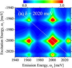
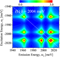
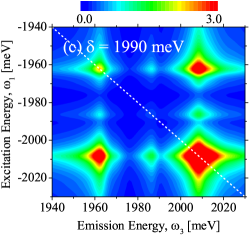
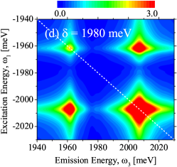
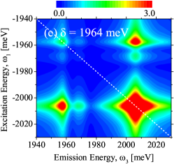
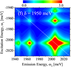
Figure 6: The simulated rephasing 2D coherent spectra (amplitude) at various photon detunings and at zero mixing time decays $t_{2}=0$. The photon detuning decreases from $\delta=2020$ meV to from $\delta=1950$ meV in (a)-(f). We typically find three peaks appearing on the diagonal dashed line. The red color illustrates the maximum amplitude, as indicated in the colormap above each subplot. The electron Fermi energy is set to be $\varepsilon_{F}=7.8$ meV.

IV.1 Zero mixing time delay $t_{2}=0$

Let us first focus on the case of zero mixing time delay $t_{2}=0$, where

$$\mathcal{S}\left(\omega_{1},0,\omega_{3}\right)=2\sum_{nm}\frac{Z_{X}^{(n)}}{\left(-\omega_{1}\right)^{-}-\mathcal{E}^{(n)}}\frac{Z_{X}^{(m)}}{\omega_{3}^{+}-\mathcal{E}^{(m)}},$$ (37)

and consider the dependence of the 2DCS spectrum $\left|\mathcal{S}(\omega_{1},0,\omega_{3})\right|$ on the photon detuning $\delta$, as shown in Fig. 6. By changing $\delta$ from the blue shift above the exciton-polariton crossing (a) to the red shift below the trion-polariton crossing (f), we typically find three diagonal peaks located at the diagonal line $\omega_{3}=-\omega_{1}$ (see the white dashed lines) and six off-diagonal cross-peaks located symmetrically with respect to the diagonal line.

These peaks arise from the three branches of excitations, as we already seen in Fig. 1. Formally, with decreasing energy the many Fermi-polaron-polariton states have been grouped into the upper polariton, middle polariton, and lower polariton branches, as often referred to in the literature Sidler2017 ; Tan2020 ; Rana2021 ; BastarracheaMagnani2021 ; Zhumagulov2022 . Therefore, we can roughly understand the Fermi-polaron-polariton as a three-energy-level system, with the energies $\mathcal{E}^{(n)},\mathcal{E}^{(m)}\sim E_{UP}$, $E_{MP}$, and $E_{LP}$ that are tunable by the cavity photon detuning. The corresponding excitonic weights are given by the excitonic residues $Z_{X}^{(UP)}$, $Z_{X}^{(MP)}$, and $Z_{X}^{(LP)}$. Hence, from Eq. (37) we can easily identify that the diagonal peaks occur when $\omega_{1}=-E_{\alpha}$ and $\omega_{3}=E_{\alpha}$ with peak amplitude $(Z_{X}^{(\alpha)})^{2}$ ($\alpha=UP,MP,LP$), while the off-diagonal peaks appear when $\omega_{1}=-E_{\alpha}$ and $\omega_{3}=E_{\beta}$ with peak amplitude $Z_{X}^{(\alpha)}Z_{X}^{(\beta)}$ ($\alpha\neq\beta=UP,MP,LP$).

The experimental measurement of diagonal peaks and crossover peaks at zero mixing time delay $t_{2}=0$ then provides us the information of both the energies $E_{\alpha}$ and the residues $Z_{X}^{(\alpha)}$. In particular, when the photon detuning $\delta$ is near the two avoided crossings (as shown in Fig. 6(b) and 6(e), respectively), we may easily identify the effective Rabi coupling from the corresponding energy splitting. Near the avoided crossing for the trion-polariton, the asymmetry of the crossing can also be clearly seen.

We note that, when the photon detuning is tuned to roughly the half-way between the two avoided crossing, the middle polariton disappears in the 2DCS spectrum (see Fig. 6(d)). This is simply because, at this detuning the middle polariton is of photonic in characteristics, with negligible excitonic component. Therefore, it can not be seen from the 2DCS, which probes the excitonic part instead of the photonic part of the system. This feature of the 2DCS spectrum is useful to characterize the main component of the ground-state of the trion-polariton (or the lower polariton branch). As the photon detuning decreases across the avoided crossing for trion-polaritons, we find that the brightness of the diagonal trion-polariton peak becomes much weaker.

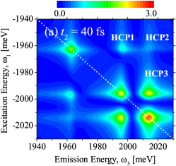
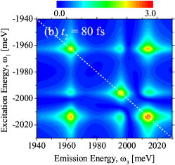
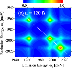
t

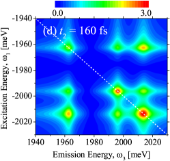
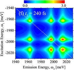
Figure 7: The simulated rephasing 2D coherent spectra (amplitude) at the photon detuning $\delta=2004$ meV with increasing mixing time decays $t_{2}$ from (a) to (f). In (a), the three higher-cross-peak (HCP) are indicated. The three peaks appearing on the diagonal dashed line essentially do not change. However, the higher-cross-peaks and lower-cross peaks oscillate as a function of $t_{2}$, revealing the quantum coherence among different quasiparticles. The red color illustrates the maximum amplitude, as indicated in the colormap above each subplot. The electron Fermi energy is set to be $\varepsilon_{F}=7.8$ meV.

Although the upper, middle and lower polariton branches can also be conveniently measured by using one-dimensional optical response, such as the reflectance spectroscopy and photoluminescence spectroscopy Sidler2017 , the application of 2DCS spectroscopy has unique features to discriminate the intrinsic homogeneous line-with of the resonance peaks Hao2016NanoLett and the interaction effects Li2006 ; Muir2022 . Unfortunately, both effects (i.e., the disorder potential for excitons and the exciton-exciton interaction) are not included in our model Hamiltonian. Nevertheless, our results in Fig. 6 provide the essential qualitative features of the 2DCS spectrum, which is to be measured in future exciton-polariton experiments. In addition, the appearance of the off-diagonal peaks and their evolution as a function of the mixing time decay $t_{2}$ are useful to characterize the quantum coherences among the different branches of polaritons, which we now turn to discuss.

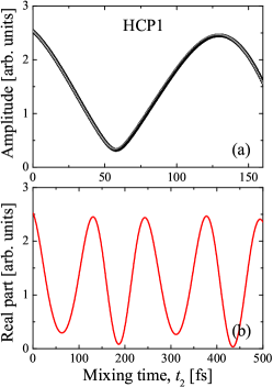
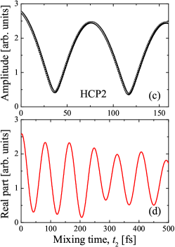
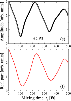
Figure 8: The simulated amplitude (a) and real part (b) of the rephasing 2D signal at the three cross-peaks as a function of the mixing time delays $t_{2}$. Note the different periodicity at different crosspeaks. We choose the photon detuning $\delta=2004$ meV as in Fig. 6 and take the electron Fermi energy $\varepsilon_{F}=7.8$ meV.

IV.2 Quantum coherence of the cross-peaks

In Fig. 7, we present the simulated rephasing 2D coherent spectra $\left|\mathcal{S}(\omega_{1},t_{2},\omega_{3})\right|$ with increasing mixing time decays $t_{2}$. We choose a photon detuning $\delta=2004$ meV at the avoided crossing for exciton-polaritons, where all the three polariton branches are clearly visible at $t_{2}=0$. We label the three off-peaks at the top-right corner of the figure as HCP1, HCP2 and HCP3 Hao2016NanoLett , respectively.

As can be seen from Eq. (36), the time $t_{2}$-dependence of the 2D spectrum $\mathcal{S}\left(\omega_{1},t_{2},\omega_{3}\right)$ comes in through the term $e^{i\left[\mathcal{E}^{(n)}-\mathcal{E}^{(m)}\right]t_{2}}$. As we interpret the Fermi-polaron-polariton as a three-level system, where the energy levels $\mathcal{E}^{(n)},\mathcal{E}^{(m)}$ are to be replaced by $E_{UP}$, $E_{MP}$, and $E_{LP}$, it is readily seen that the $t_{2}$-term gives rise to quantum oscillations with three different periods: $2\pi/\left|E_{MP}-E_{LP}\right|$ for the HCP1 cross-peak, $2\pi/\left|E_{UP}-E_{LP}\right|$ for HCP2, and $2\pi/\left|E_{UP}-E_{MP}\right|$ for HCP3. At the photon detuning $\delta=2004$ meV, we find that $E_{MP}-E_{LP}\simeq 33.2$ meV, $E_{UP}-E_{LP}\simeq 50.5$ meV, and $E_{UP}-E_{MP}\simeq 17.3$ meV. Therefore, the periodicities of the cross-peaks are at the order of $10^{-10}$ s or $100$ fs, and are given by $T_{\textrm{HCP1}}\simeq 124.4$ fs, $T_{\textrm{HCP2}}\simeq 81.6$ fs, and $T_{\textrm{HCP3}}\simeq 239.5$ fs.

The 2DCS spectra in Fig. 7 are shown in $40$ fs increments. We can clearly identify that the brightness of each cross-peak oscillates with the mixing time delay $t_{2}$, revealing the coherent coupling among different branches of exciton-polariton and trion-polaritons. In comparison with the zero mixing time delay 2DCS in Fig. 6(b), we find that the HPC1 cross-peak nearly recovers its full brightness at $t_{2}=120$ fs and $240$ fs, confirming that its periodicity is close to the anticipated value $T_{\textrm{HCP1}}\simeq 124.4$ fs. For the HCP2 cross-peak, we see similarly that it nearly disappears at $t_{2}=40$ fs, $120$ fs and $200$ fs and fully recovers at t $t_{2}=80$ fs, $160$ fs and $240$ fs, in agreement with our anticipation that $T_{\textrm{HCP2}}\simeq 81.6$ fs. In addition, the HPC3 cross-peak only returns to the its full brightness at $T_{\textrm{HCP3}}\simeq 240$ fs.

To better characterize the quantum oscillations, we report in Fig. 8 the simulated rephasing 2D signal at the crosspeaks as a function of the mixing time $t_{2}$, both in the form of its amplitude (the upper panel) and in its real part (the lower panel). The oscillations do not take the exact form of $1+\cos(\omega t_{2})$, as one may naively anticipate from Eq. (36). This is partly due to the existence and competition of three different periods in the oscillations, which may bring a slight irregular structure. On the other hand, we find that the oscillations at HCP2 and HCP3 typically exhibit a decay. These dampings should be related to the many-body nature of the upper-polariton branch, i.e., it is formed by a bundle of many-body states as we discussed in Fig. 2. Therefore, the upper polariton has an intrinsic spectral broadening, which eventually causes the damping in the quantum oscillation of the cross-peaks HCP2 and HCP3. In contrast, both the lower-polariton and middle-polariton at the detuning $\delta=2004$ meV are dominated by a single Fermi polaron state, and do not experience the intrinsic spectral broadening. As a result, the quantum oscillation at HCP1 is long-lived, if we do not take into account the lifetimes of excitons (due to the natural radiative decay) and of photons (due to the quality of the cavity).

V Conclusions and outlooks

In conclusions, based on the Fermi polaron description of an exciton-polariton immersed in an electron gas, we have analyzed the structure of exciton-polaritons and trion-polaritons in monolayer transition metal dichalcogenides and have predicted their 2D coherent spectroscopy for on-going experimental explorations in the near future.

From the structure analysis, we have found that the upper-polariton branch at the exciton-polariton avoided crossing typically consists of a number of many-body Fermi polaron states. Instead, the lower-polariton branch at the trion-polariton avoided crossing involves only one Fermi polaron state. The situation for the middle-polariton branch varies, depending on whether it is close to the exciton-polariton crossing or close to the trion-polariton crossing. In the former case, the middle-polariton is also dominated by a single Fermi polaron state.

As there are three polariton branches Sidler2017 ; Rana2021 ; Zhumagulov2022 , in the 2D coherent spectroscopy we have found three diagonal peaks and six off-diagonal cross-peaks. From these peaks measured in future experiments, in principle we should be able to extract the excitonic residues of different polariton branches. We have predicted the existence of quantum oscillations in the 2D spectra as a function of the mixing time delay $t_{2}$, as the evidence for the quantum coherence among the different polariton branches Hao2016NanoLett .

Although in the present study we have not considered the effects of the disorder potential on excitons and the inter-exciton interaction, our results would provide a good starting point to understand the 2D coherent spectroscopy on exciton-polaritons to be experimentally measured in the near future. Theoretically, the inclusions of the disorder effect and interaction effect would be extremely challenging in numerics, since the dimension of the Hilbert space of the model Hamiltonian will increase dramatically. We will address these effects in future publications.

VI Statements and Declarations

VI.0.1 Ethics approval and consent to participate

Not Applicable.

VI.0.2 Consent for publication

Not Applicable.

VI.0.3 Availability of data and materials

The data generated during the current study are available from the contributing author upon reasonable request.

VI.0.4 Competing interests

The authors have no competing interests to declare that are relevant to the content of this article.

VI.0.5 Funding

This research was supported by the Australian Research Council’s (ARC) Discovery Program, Grants No. DE180100592 and No. DP190100815 (J.W.), and Grant No. DP180102018 (X.-J.L).

VI.0.6 Authors’ contributions

All the authors equally contributed to all aspects of the manuscript. All the authors read and approved the final manuscript.

VI.0.7 Acknowledgements

See funding support.

VI.0.8 Authors’ information

Hui Hu, Centre for Quantum Technology Theory, Swinburne University of Technology, Melbourne 3122, Australia, Email: hhu@swin.edu.au

Jia Wang, Centre for Quantum Technology Theory, Swinburne University of Technology, Melbourne 3122, Australia, Email: jiawang@swin.edu.au

Riley Lalor, Centre for Quantum Technology Theory, Swinburne University of Technology, Melbourne 3122, Australia, Email:103192654@student.swin.edu.au

Xia-Ji Liu, Centre for Quantum Technology Theory, Swinburne University of Technology, Melbourne 3122, Australia, Email: xiajiliu@swin.edu.au

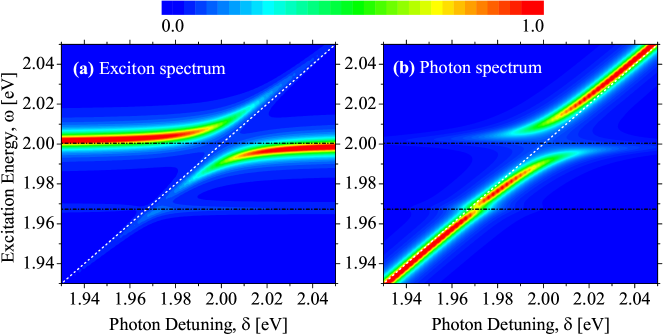
Figure 9: Two-dimensional contour plots of the zero-momentum spectral functions of the exciton (a) and of the photon (b), as a function of the photon detuning $\delta$ at a small electron Fermi energy $\varepsilon_{F}=1.0$ meV. The two black horizontal dot-dashed lines show the energies of the exciton (i.e., the repulsive polaron branch with $\varepsilon_{X}\simeq 2000.4$ meV) and the trion (i.e., the attractive polaron branch with $\varepsilon_{T}\simeq 1967.4$ meV), in the absence of the cavity photon field. The diagonal white dotted line indicates the photon detuning $\omega=\delta$. At this low electron density, the avoided crossing at $\omega=E_{T}$ is insignificant. The spectral functions are measured in arbitrary units and are plotted in a linear scale..

Appendix A Exciton-polaritons and trion-polaritons at small electron density

In Fig. 9, we report the zero-momentum spectral functions of excitons and of photons for a small electron density with Fermi energy $\varepsilon_{F}=1.0$ meV. At this density, the exciton energy level is barely affected by the scattering with the electron gas and the trion energy level is basically given by the trion binding energy of $E_{T}\simeq 32$ meV. We can hardly identify the existence of the trion-polariton from the excitonic spectrum. Neither, the trion-polariton can barely be seen from the photonic spectrum. Both spectra are very similar to the spectrum of exciton-polaritons in the absence of the electron gas.

References

- (1) H. Deng, H. Haug, and Y. Yamamoto, Exciton-polariton Bose-Einstein condensation, Rev. Mod. Phys. 82, 1489 (2010).
- (2) I. Carusotto and C. Ciuti, Quantum fluids of light, Rev. Mod. Phys. 85, 299 (2013).
- (3) T. Byrnes, N. Y. Kim, and Y. Yamamoto, Exciton-polariton condensates, Nat. Phys. 10, 803 (2014).
- (4) K. S. Novoselov, D. Jiang, F. Schedin, T. J. Booth, V. V. Khotkevich, S. V. Morozov, and A. K. Geim, Two-dimensional atomic crystals, Proc. Natl. Acad. Sci. U.S.A. 102, 10451 (2005).
- (5) G. Wang, A. Chernikov, M. M. Glazov, T. F. Heinz, X. Marie, T. Amand, and B. Urbaszek, Colloquium: Excitons in atomically thin transition metal dichalcogenides, Rev. Mod. Phys. 90, 021001 (2018).
- (6) T. C. Berkelbach and D. R. Reichman, Optical and Excitonic Properties of Atomically Thin Transition-Metal Dichalcogenides, Annu. Rev. Condens. Matter Phys. 9, 379 (2018).
- (7) H. Hu, H. Deng, and X.-J. Liu, Polariton-polariton interaction beyond the Born approximation: A toy model study, Phys. Rev. A 102, 063305 (2020).
- (8) M. Sidler, P. Back, O. Cotlet, A. Srivastava, T. Fink, M. Kroner, E. Demler, and A. Imamoglu, Fermi polaron-polaritons in chargetunable atomically thin semiconductors, Nat. Phys. 13, 255 (2017).
- (9) D. K. Efimkin and A. H. MacDonald, Many-body theory of trion absorption features in two-dimensional semiconductors, Phys. Rev. B 95, 035417 (2017).
- (10) P. Massignan, M. Zaccanti, and G. M. Bruun, Polarons, dressed molecules and itinerant ferromagnetism in ultracold Fermi gases, Rep. Prog. Phys. 77, 034401 (2014).
- (11) R. Schmidt, M. Knap, D. A. Ivanov, J.-S. You, M. Cetina, and E. Demler, Universal many-body response of heavy impurities coupled to a Fermi sea: a review of recent progress, Rep. Prog. Phys. 81, 024401 (2018).
- (12) J. Wang, X.-J. Liu, and H. Hu, Exact Quasiparticle Properties of a Heavy Polaron in BCS Fermi Superfluids, Phys. Rev. Lett. 128, 175301 (2022).
- (13) J. Wang, X.-J. Liu, and H. Hu, Heavy polarons in ultracold atomic Fermi superfluids at the BEC-BCS crossover: Formalism and applications, Phys. Rev. A 105, 043320 (2022).
- (14) L. B. Tan, O. Cotlet, A. Bergschneider, R. Schmidt, P. Back, Y. Shimazaki, M. Kroner, and A. İmamoğlu, Interacting Polaron-Polaritons, Phys. Rev. X 10, 021011 (2020).
- (15) F. Rana, O. Koksal, M. Jung, G. Shvets, A. N. Vamivakas, and C. Manolatou, Exciton-Trion Polaritons in Doped Two-Dimensional Semiconductors, Phys. Rev. Lett. 126, 127402 (2021).
- (16) M. A. Bastarrachea-Magnani, A. Camacho-Guardian, and G. M. Bruun, Attractive and Repulsive Exciton-Polariton Interactions Mediated by an Electron Gas, Phys. Rev. Lett. 126, 127405 (2021).
- (17) K. W. Song, S. Chiavazzo, I. A. Shelykh, and O. Kyriienko, Attractive trion-polariton nonlinearity due to Coulomb scattering, arXiv:2204.00594 (2022).
- (18) D. Jonas, Two-Dimensional Fermtosecond Spectroscopy, Ann. Rev. Phys. Chem. 54, 425 (2003).
- (19) X. Li, T. Zhang, C. N. Borca, and S. T. Cundiff, Many-Body Interactions in Semiconductors Probed by Optical Two-Dimensional Fourier Transform Spectroscopy, Phys. Rev. Lett. 96, 057406 (2006).
- (20) M. Cho, Coherent Two-Dimensional Optical Spectroscopy, Chem. Rev. 108, 1331 (2008).
- (21) K. Hao, L. Xu, P. Nagler, A. Singh, K. Tran, C. K. Dass, C. Schuller, T. Korn, X. Li, and G. Moody, Coherent and incoherent coupling dynamics between neutral and charged excitons in monolayer MoSe2, Nano Lett. 16, 5109 (2016).
- (22) J. B. Muir, J. Levinsen, S. K. Earl, M. A. Conway, J. H. Cole, M. Wurdack, R. Mishra, D. J. Ing, E. Estrecho, Y. Lu, D. K. Efimkin, J. O. Tollerud, E. A. Ostrovskaya, M. M. Parish, and J. A. Davis, Exciton-polaron interactions in monolayer WS2, Nat. Commun. 13, 6164 (2022).
- (23) F. Chevy, Universal phase diagram of a strongly interacting Fermi gas with unbalanced spin populations, Phys. Rev. A 74, 063628 (2006).
- (24) H. Hu and X.-J. Liu, Fermi polarons at finite temperature: Spectral function and rf spectroscopy, Phys. Rev. A 105, 043303 (2022).
- (25) Y. V. Zhumagulov, S. Chiavazzo, D. R. Gulevich, V. Perebeinos, I. A. Shelykh, and O. Kyriienko, Microscopic theory of exciton and trion polaritons in doped monolayers of transition metal dichalcogenides, npj Comput Mater 8, 92 (2022).
- (26) R. Tempelaar and T. C. Berkelbach, Many-body simulation of two-dimensional electronic spectroscopy of excitons and trions in monolayer transition metal dichalcogenides, Nat. Commun. 10, 3419 (2019).
- (27) L. P. Lindoy, Y.-W. Chang, and D. R. Reichman, Two-dimensional spectroscopy of two-dimensional materials, arXiv:2206.01799 (2022).
- (28) J. Wang, Multidimensional Spectroscopy of Time-Dependent Impurities in Ultracold Fermions, arXiv:2207.10501 (2022).
- (29) J. Wang, H. Hu, and X.-J. Liu, Two-dimensional spectroscopic diagnosis of quantum coherence in Fermi polarons, arXiv:2207.14509 (2022).
- (30) H. Hu, J. Wang, and X.-J. Liu, Microscopic many-body theory of two-dimensional coherent spectroscopy of excitons and trions in atomically thin transition metal dichalcogenides, arXiv:2208.03599 (2022).