Time evolution of nonadditive entropies: The logistic map

Abstract

Due to the second principle of thermodynamics, the time dependence of entropy for all kinds of systems under all kinds of physical circumstances always thrives interest. The logistic map $x_{t+1}=1-ax_{t}^{2}\in[-1,1]\;(a\in[0,2])$ is neither large, since it has only one degree of freedom, nor closed, since it is dissipative. It exhibits, nevertheless, a peculiar time evolution of its natural entropy, which is the additive Boltzmann-Gibbs-Shannon one, $S_{BG}=-\sum_{i=1}^{W}p_{i}\ln p_{i}$, for all values of $a$ for which the Lyapunov exponent is positive, and the nonadditive one $S_{q}=\frac{1-\sum_{i=1}^{W}p_{i}^{q}}{q-1}$ with $q=0.2445\dots$ at the edge of chaos, where the Lyapunov exponent vanishes, $W$ being the number of windows of the phase space partition. We numerically show that, for increasing time, the phase-space-averaged entropy overshoots above its stationary-state value in all cases. However, when $W\to\infty$, the overshooting gradually disappears for the most chaotic case ($a=2$), whereas, in remarkable contrast, it appears to monotonically diverge at the Feigenbaum point ($a=1.4011\dots$). Consequently, the stationary-state entropy value is achieved from above, instead of from below, as it could have been a priori expected. These results raise the question whether the usual requirements – large, closed, and for generic initial conditions – for the second principle validity might be necessary but not sufficient.

.1 1 - Introduction

Molecular physics may be seen as a more detailed description of solidly established laws of chemistry. Analogously, atomic physics may be seen as a more detailed description of solidly established laws of molecular physics. Nuclear physics, physics of elementary particles, evolve along the same lines. Epistemologically, it is tacitly required that, at each deeper and deeper description, the knowledge previously established on solid grounds is satisfactorily recovered at some adequate scale. Another paradigmatic example of the same path is general relativity which, in the $G\to 0$ limit, recovers special relativity, which in turn recovers, in the $c\to\infty$ limit, Newtonian mechanics. Analogously, quantum mechanics recovers, in the $\hbar\to 0$ limit, Newtonian mechanics. On the experimental world, optic microscopy was improved by electronic microscopy, in turn improved by scanning probe microscopy, and so on. The celebrated sentence “If I have seen further it is by standing on the shoulders of giants” that Isaac Newton included in his letter to Robert Hooke dramatically illustrates that same path. This is essentially how, along the years and centuries, the progress of sciences proceeds along the footprints of what was previously established on reliable bases.

In the realm of statistical mechanics, where the concept of coarse graining, hence of changements of scales, plays a foundational role, a similar path is being followed since its formulation in the XIXth century, and also along the last three-four decades. The pioneering works of Boltzmann and Gibbs Boltzmann1872 ; Boltzmann1877 ; Gibbs1901 established, upon undeniably solid bases, a magnificent theory which is structurally associated with the Boltzmann-Gibbs (BG) entropic functional

$$S_{BG}=-k\sum_{i=1}^{W}p_{i}\ln p_{i}\;\;(\sum_{i=1}^{W}p_{i}=1)\,,$$ (1)

and consistent expressions for continuous or quantum variables, $k$ being a conventional positive constant adopted once forever (in physics, $k$ is chosen to be the Boltzmann constant $k_{B}$; in information theory and computational sciences, it is frequently adopted $k=1$).

In the simple case of equal probabilities, this entropic functional is given by $S_{BG}=k\ln W$. Eq. (1) is generically additive Penrose1970 . Indeed, if $A$ and $B$ are two probabilistically independent systems (i.e., $p_{ij}^{A+B}=p_{i}^{A}p_{j}^{B}$), we straightforwardly verify that $S_{BG}(A+B)=S_{BG}(A)+S_{BG}(B)$. This celebrated entropic functional is consistent with thermodynamics for all systems whose $N$ elements are either independent or weakly interacting in the sense that only basically local (in space/time) interactions are involved. For example, if we have equal probabilities and the system is such that the number of accessible microscopic configurations is given by $W(N)\propto\mu^{N}\;(\mu>1;\,N\to\infty)$, then $S_{BG}(N)$ is extensive as required by thermodynamics. Indeed $S_{BG}(N)=k\ln W(N)\sim k(\ln\mu)N$. But if the correlations are nonlocal in space/time, $S_{BG}$ may become thermodynamically inadequate. Such is the case of equal probabilities with say $W(N)\propto N^{\nu}\;(\nu>0;\,N\to\infty)$: it immediately follows $S_{BG}(N)\propto\ln N$, which violates thermodynamical extensivity. To satisfactorily approach cases such as this one, it was proposed in 1988 Tsallis1988 ; TsallisMendesPlastino1998 ; GellMannTsallis2004 ; Tsallis2009 to build a more general statistical mechanics based on the nonadditive entropic functional

$$S_{q}\equiv k\frac{1-\sum_{i=1}^{W}p_{i}^{q}}{q-1}=k\sum_{i=1}^{W}p_{i}\ln_{q}\frac{1}{p_{i}}=-k\sum_{i=1}^{W}p_{i}^{q}\ln_{q}p_{i}=-k\sum_{i=1}^{W}p_{i}\ln_{2-q}p_{i}\;\;(q\in\mathbb{R};S_{1}=S_{BG})\,,$$ (2)

with $\ln_{q}z\equiv\frac{z^{1-q}-1}{1-q}\;(\ln_{1}z=\ln z)$ and its inverse $e_{q}^{z}\equiv[1+(1-q)z]_{+}^{1/(1-q)}$; ($e_{1}^{z}=e^{z}$; $[z]_{+}=z$ if $z>0$ and vanishes otherwise); for $q<0$, it is necessary to exclude from the sum the terms with vanishing $p_{i}$. We easily verify that equal probabilities yield $S_{q}=k\ln_{q}W$, and that generically we have

$$\frac{S_{q}(A+B)}{k}=\frac{S_{q}(A)}{k}+\frac{S_{q}(B)}{k}+(1-q)\frac{S_{q}(A)}{k}\frac{S_{q}(B)}{k}\,,$$ (3)

hence

$$S_{q}(A+B)=S_{q}(A)+S_{q}(B)+\frac{1-q}{k}S_{q}(A)S_{q}(B)\,.$$ (4)

Consequently, in the $(1-q)/k\to 0$ limit, we recover the $S_{BG}$ additivity. For the anomalous class of systems mentioned above, namely $W(N)\propto N^{\nu}$, we obtain, $\forall\nu$, the extensive entropy $S_{1-1/\nu}(N)=k\ln_{1-1/\nu}W(N)\propto N$, as required by the Legendre structure of thermodynamics (see Tsallis2009 ; TsallisCirto2013 ; Tsallis2022 and references therein).

At this point let us remind that a general entropic functional $S_{G}(\{p_{i}\})$ is defined as trace-form if it can be written as $S_{G}=k\sum_{i=1}^{W}f(p_{i})\equiv k\sum_{i=1}^{W}p_{i}\,g(p_{i})$. A $G$-generalized logarithm can be defined as $g(p_{i})\equiv\ln_{G}(1/p_{i})$. Consequently $S_{G}=k\langle\sigma_{i}\rangle$, where $\sigma_{i}\equiv\ln_{G}(1/p_{i})$ is the surprise Watanabe1969 or unexpectedness Barlow1990 ; $\sigma(p)$ is assumed to monotonically increase, when $p_{i}$ decreases from 1 to 0, from 0 to its maximum value (which may be infinity). Only trace-form entropies can be written as the mean value of a surprise.

Moreover, an entropic functional $S(\{p_{i}\};\{\eta\})$ is said composable if it satisfies, for two probabilistically independent systems $A$ and $B$, the property $\frac{S(A+B)}{k}=F(\frac{S(A)}{k},\frac{S(B)}{k};\{\eta\})$, where $\{\eta\}$ is a set of fixed indices characterizing the functional (e.g., for $S_{q}$, it is $\{\eta\}\equiv q$ ); we use the notation $\{0\}$ to indicate absence of any such index. $F(x,y;\{\eta\})$ is a smooth function of $(x,y)$ which depends on a (typically small) set of universal indices $\{\eta\}$ defined in such a way that $F(x,y;\{0\})=x+y$ (additivity), which corresponds to the BG entropy. Additionally, $F(x,y;\{\eta\})$ is assumed to satisfy $F(x,0;\{\eta\})=x$ (null-composability), $F(x,y;\{\eta\})=F(y,x;\{\eta\})$ (symmetry), $F(x,F(y,z;\{\eta\});\{\eta\})=F(F(x,y;\{\eta\}),z;\{\eta\})$ (associativity) (see details and thermodynamical motivation in Tsallis2009 ; Tsallis2022 ).

We specially focus here on $S_{q}$ because the Enciso-Tempesta theorem EncisoTempesta2017 proves that this entropic functional is the unique one which is simultaneously trace-form, composable, and contains $S_{BG}$ as a particular case.

In the present paper, we numerically exhibit the above mentioned epistemological path on the time evolution of $S_{q}$(t) associated with the paradigmatic one-dimensional dissipative logistic map. Through appropriate scaling of successively finer partitions of the phase-space into $W$ equal windows, we verify that, for both strong and weak chaos, properties such as the entropy production per unit time and related phenomenology are satisfied.

The logistic map is defined as follows:

$$x_{t+1}=1-ax_{t}^{2}\;(x_{t}\in[-1,1];\,a\in[0,2];t=0,1,2,\cdots)\,.$$ (5)

Depending on the value of the external parameter $a$, the corresponding Lyapunov exponent $\lambda$ can be positive, negative or zero. When $\lambda>0$ we say that the system is strongly chaotic: the simplest, and strongest, such case emerges for $a=2$, which implies $\lambda=\ln 2>0$. When $\lambda=0$ and the corresponding value of $a$, noted $a_{c}$, is located at the accumulation point of successive bifurcations, we say that the system is weakly chaotic. The most studied such points occur at the edge of chaos, more precisely, at the so-called Feigenbaum-Coullet-Tresser point, with $a_{c}=1.40115518909205\dots$. In all cases, if we start from initial conditions such that the entropy nearly vanishes at $t=0$, we observe that, for all values of $q$, $S_{q}$ tends to increase (not necessarily in a monotonic manner) as time increases. But it tends to increase linearly (thus providing a finite entropy production per unit time) only for an unique value of the index $q$. For $a=2$, the entropy which linearly increases with time, thus yielding a finite entropy production per unit time (satisfying the Pesin identity for the entropy production per unit time $K_{BG}\equiv\lim_{t\to\infty}S_{BG}(t)/t=\lambda$), is $S_{BG}$. In contrast, at the edge of chaos, the entropy which linearly increases with time is $S_{q}$ with $q=q_{c}\equiv 0.24448770134128\dots$. In fact, depending on the initial conditions, there are infinitely many such linearities (see LyraTsallis1998 ; BaldovinRobledo2004 ; MayoralRobledo2005 ; Robledo2006 and references therein). This is why we present here the corresponding mean values over a natural set of initial conditions, similarly to what has been calculated in AnanosTsallis2004 .

.2 2 - Strong and weak chaos

We partition the interval $x\in[-1,1]$ into $W$ equal little windows, and uniformly choose $M$ initial conditions, typically $M=10W$ (this number of initial conditions is sufficiently high for attaining proper estimates of entropies. In fact, the relative error $\epsilon=\frac{1}{t_{\text{max}}}\sum_{t=1}^{t_{\text{max}}}\frac{|S_{q_{c}}(M=10W;t)-S_{q_{c}}(M=100W;t)|}{S_{q_{c}}(M=100W;t)}$ estimated with higher number of initial conditions, e.g. $M=100W$ and $t_{\text{max}}=10000$ is $\epsilon<2\times 10^{-3}$), within one such interval (noted $j$). We denote $\{p_{i}\}\,(i=1,2,\cdots,W)$ the occupancy probabilities of all $W$ windows. At $t=0$, we have $p_{j}=1$ for the selected window, and $p_{i\neq j}=0$ for all the other $(W-1)$ windows. Consequently $S_{q}(t)$ satisfies $S_{q}(0)=0\,,\forall q$. For $a=2$, the only value of $q$ for which we have a linear growth while approaching saturation is $q=1$ (this procedure was initially proposed in LatoraBarangerRapisardaTsallis2000 ). We then repeat the operation for each one of the $W$ windows, and finally average the data for $S_{q}$: see Figs. 1 and 2.

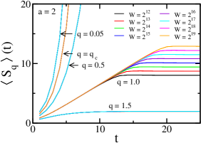
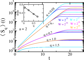
Figure 1: (Color online) Time dependence of the average $\langle S_{1}\rangle$ for $a=2$. Left: Linear-linear representation. The slope of the linear part equals $\lambda=\ln 2$, consistently with the Pesin identity. For all values of $q\neq 1$, several values of $W$ yield curves that are superimposed, and consequently can not be clearly identified. Right: Log-linear representation. We verify that, for $q<1$, a purely exponential behavior gradually emerges before saturation. Inset: The extrapolated slope for $q=0$ yields $0.69$.

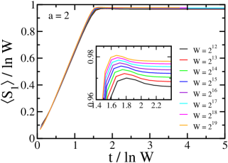
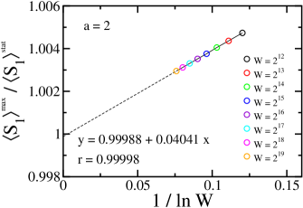
Figure 2: (Color online) Left: Data collapse of the results indicated in Fig. 1. The maxima observed here are consistent with Fig. 1 of BorgesTsallisAnanosOliveira2002 . Right: Extrapolation of the ratios.

We apply the same numerical procedure described above for $a=a_{c}$: see Figs. 3, 4 and 5.

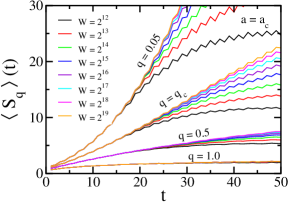
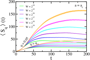
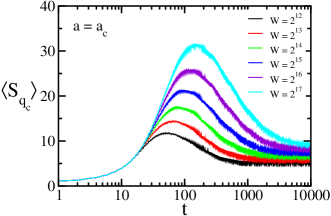
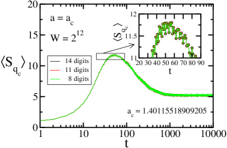
Figure 3: (Color online) Time dependence of the average $\langle S_{q}\rangle$ for $a=a_{c}$. Strictly speaking, for the system to live (depending on the initial condition and assuming that all calculations are done with infinite digits) on a multifractal, it is necessary to know $a_{c}$ with infinite digits, which is of course impossible. By varying the numerical precision that we have presently used for $a_{c}$, we have verified that this effect is numerically negligible for the number of digits within which our calculations have been done (see bottom-right plot).

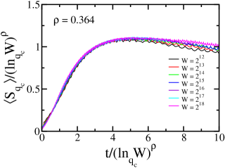
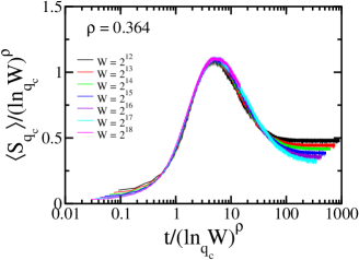
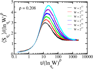
Figure 4: (Color online) Data collapse of the results indicated in Fig. 3. Notice that, for $q<1$, $\rho>0$ and $W\gg 1$, $(\ln_{q}W)^{\rho}\sim[W^{1-q}/(1-q)]^{\rho}\propto W^{(1-q)\rho}$, which reveals the (multi) fractal origin of $\rho$ (in the sense that $\rho$ is not an integer number). For $q\neq q_{c}$, there is no value of $\rho$ for which all the $a=a_{c}$ data can be collapsed through a single scaling with $(\ln_{q}W)^{\rho}$. Top left: Linear-linear representation aiming the collapse, for increasing $W$, of the maxima; the slope at first inflection point, located at $0.97\pm 0.02$, is $0.47\pm 0.01$; $\langle S_{q_{c}}\rangle/(\ln_{q_{c}}W)^{\rho}$ attains its maximal value $1.1\pm 0.01$ at $t/(\ln_{q_{c}}W)^{\rho}=5.3\pm 0.3$, with $\rho=0.364\pm 0.003$. Top right: The same as in Top-left but in linear-log representation. Bottom: Linear-log representation aiming the collapse, for increasing $W$, of the stationary-state heights; this collapse occurs at height $=1.35\pm 0.04$ with $\rho=0.208\pm 0.002$.

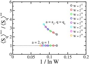
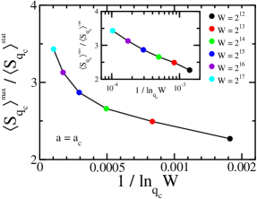
Figure 5: (Color online) $W\to\infty$ extrapolations of the maxima. Left: Abscissa scaled with $\ln W$. Right: Abscissa scaled with $\ln_{q_{c}}W$. The data suggest that $\lim_{W\to\infty}[\langle S_{q}\rangle^{\text{max}}/\langle S_{q}\rangle^{\text{stat}}]$ equals unity for $(a,q)=(2,1)$ and diverges for $(a,q)=(a_{c},q_{c})$.

Before concluding, let us emphasize that the robustness of the peaks in the time evolution of the entropy $S_{q}$ at $a=a_{c}$ has been numerically verified under four different circumstances, namely with regard to (i) the number of initial conditions within each one of the $W$ windows (Fig. 6); (ii) the precision used in the value of $a_{c}$ (bottom-right plot in Fig. 3); (iii) variations of the occupancy of phase space in the neighborhood of the multifractal attractor at $a=a_{c}$ (Fig. 7); (iv) variations of the map (Fig. 8).

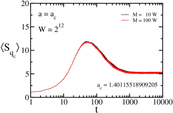
Figure 6: (Color online) Influence of the number of initial conditions within each of the $W$ windows. Instance with $W=2^{12}$ windows with two cases: $M=10W$ initial conditions (black) and $M=100W$ initial conditions (red). The similarity of the curves indicate that $M=10W$ is a sufficiently large number of initial conditions for the purposes of the calculations.

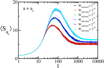
Figure 7: (Color online) Influence of the phase-space occupation in the neighborhood of the multifractal attractor at $a=a_{c}$ (see RobledoMoyano2009 ). Uniform means that all the $W$ windows start with the same number of initial conditions; alternate means that the occupancy of each of the $W$ windows starts alternating the double of initial conditions and emptiness, the total number $WM$ of initial conditions in the interval $[-1,1]$ remaining the same.

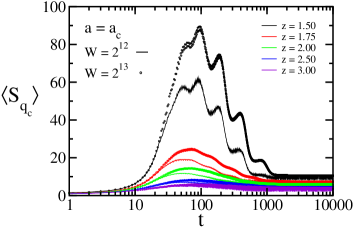
Figure 8: (Color online) Peaks corresponding to the $z$-logistic map $x_{t+1}=1-a|x_{t}|^{z}$ for typical values of $z$. For $z=1.50,1.75,2.00,2.50,3.00$ we have $(a_{c},q_{c})=(1.295509973160,-0.15)$, $(1.355060756622,0.11)$, $(1.40115518909205,0.2444877)$, $(1.47054991523,0.39)$, $(1.52187878890,0.47)$.

.3 4 - Final remarks

At this point, a few comments are certainly timely concerning the most distinguished non-trace-form entropic functional, namely the Renyi one Renyi1961

$$S_{q}^{R}\equiv k\frac{\ln\sum_{i=1}^{W}p_{i}^{q}}{1-q}=k\frac{\ln[1+(1-q)S_{q}/k]}{1-q}\;\;(q\in\mathbb{R};\,S_{1}^{R}=S_{1}=S_{BG})\,,$$ (6)

hence

$$S_{q}^{R}/k=\ln e_{q}^{S_{q}/k}$$ (7)

and

$$S_{q}/k=\ln_{q}e^{S_{q}^{R}/k}$$ (8)

This additive (hence composable) entropic functional is, $\forall q$, a monotonic function of $S_{q}$, hence, under the same constraints, it is optimized by the same distribution which optimizes $S_{q}$. However, in contrast with $S_{q}$ which is concave for all $q>0$, $S_{q}^{R}$ is concave only for $0<q\leq 1$. In addition to that, $S_{q}$ is Lesche-stable for all $q>0$, whereas $S_{q}^{R}$ has this important experimental robustness only for its particular instance $q=1$ Lesche1982 ; Abe2002 ; AbeLescheMund2007 . Moreover, if we consider the present nontrivial case $a=a_{c}$, we have that, in the $W\to\infty$ limit, $S_{q_{c}}^{R}(t)=k\frac{\ln[1+(1-q_{c})S_{q_{c}}(t)/k]}{1-q_{c}}\propto\ln t$ for $t\gg 1$. Consequently, there is no constant finite Renyi-entropy production per unit time and, consistently, no Pesin-like identities can exist. Analogously, if we consider the stationary-state of a $N$-body system belonging to the previously mentioned anomalous class $W(N)\propto N^{\rho}$, we have that $S_{q}^{R}(N)\propto\ln N$ for any $q<1$. In other words, $S_{q}^{R}(N)$ appears to be nonextensive and the Legendre structure of thermodynamics is therefore violated.

It is worthy to mention that composability is not necessary for a finite entropy production per unit time to exist (thus possibly qualifying for a Pesin-like identity to be satisfied). Such is the case, for instance, of the Kaniadakis entropy Kaniadakis2001 which is nonadditive, non-composable, trace-form, and yields nevertheless a finite entropy production per unit time.

The relevant influence of the precision used in the calculations has been exhibited as well: see Fig. 9. More specifically, the use of simple, double or quadruple precision sensibly enhances the overshooting of the time evolution of the entropy $S_{q_{c}}(t)$ at the Feigenbaum point. To reinforce these results, it would of course be necessary to use values of $a_{c}$ and of $q_{c}$ with consistently higher precision when $W$ increases. Still, the present indications are already clear enough.

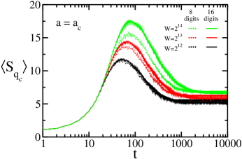
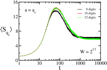
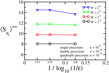
Figure 9: (Color online) Influence of the precision of the calculations. We verify that, for small values of $W$, double precision (i.e., 16 digits) is more than enough for the present purposes, but, when $W$ sensibly increases, increasingly higher precision becomes necessary. Interestingly enough, low precision underestimates the maximal value of $\langle S_{q_{c}}\rangle$, whereas it overestimates its stationary-state value.

Let us conclude by focusing on a relevant result of the present study. Our numerical simulations strongly indicate that, for both strong and weak chaos, the time behavior of $S_{q}$ ($q=1$ for $a=2$ and $q=q_{c}$ for $a=a_{c}$, respectively) at the $W\to\infty$ limit, consists in a diverging linear increase with finite slope. However, an important distinction arises on how $S_{q}(t)$ approaches its stationary-state value $S_{q}(\infty)$: it approaches from below for $a=2$, which corresponds to the naive expectation, whereas it does so from above for $a=a_{c}$, which might be considered as unexpected. This – a priori surprising – behavior is due to the fact that, for relatively early times during the present evolution at fixed $W$, the entropy system tends to approach its maximal value $\ln_{q}W$. However, for later times, the system approaches its asymptotic stationary state, which is not uniform (it is instead $U$-shaped for $a=2$ and multifractal for $a=a_{c}$).

The 2nd principle of thermodynamics is normally qualified for systems which are closed, very large, and for a generic initial situation. An intriguing question might arise: these conditions surely are necessary, but are they sufficient? Is there no need for also requiring a strongly chaotic internal dynamics (e.g., short-range interactions), which normally implies mixing and ergodicity for all or part of the system? At the light of the present results, this fundamental question appears to be an open one, surely deserving further study.

We acknowledge fruitful conversations with E.M.F. Curado and partial financial support by CNPq and Faperj (Brazilian agencies). We also acknowledge useful remarks from two anonymous referees which led to various numerical verifications of the robustness of the entropic peaks at the Feigenbaum point, thus enriching the manuscript.

References

- (1) L. Boltzmann, Weitere Studien u̇ber das Wȧrmegleichgewicht unter Gas moleku̇len [Further Studies on Thermal Equilibrium Between Gas Molecules], Wien, Ber. 66, 275 (1872).
- (2) L. Boltzmann, Uber die Beziehung eines allgemeine mechanischen Satzes zum zweiten Haupsatze der Warmetheorie, Sitzungsberichte, K. Akademie der Wissenschaften in Wien, Math.-Naturwissenschaften 75, 67-73 (1877); English translation (On the Relation of a General Mechanical Theorem to the Second Law of Thermodynamics) in S. Brush, Kinetic Theory, Vol. 2: Irreversible Processes, 188-193 (Pergamon Press, Oxford, 1966). See also K. Sharp and F. Matschinsky, Translation of Ludwig Boltzmann’s Paper “On the Relationship between the Second Fundamental Theorem of the Mechanical Theory of Heat and Probability Calculations Regarding the Conditions for Thermal Equilibrium” Sitzungberichte der Kaiserlichen Akademie der Wissenschaften. Mathematisch-Naturwissen Classe. Abt. II, LXXVI 1877, pp 373-435 (Wien. Ber. 1877, 76:373-435). Reprinted in Wiss. Abhandlungen, Vol. II, reprint 42, p. 164-223, Barth, Leipzig, 1909, Entropy 17, 1971-2009 (2015).
- (3) J.W. Gibbs, Elementary Principles in Statistical Mechanics – Developed with Especial Reference to the Rational Foundation of Thermodynamics (C. Scribner’s Sons, New York, 1902; Yale University Press, New Haven, 1948); OX Bow Press, Woodbridge, Connecticut, 1981). See also J.W. Gibbs, The collected works,Vol.1, Thermodynamics, (Yale University Press, 1948).
- (4) O. Penrose, Foundations of Statistical Mechanics: A Deductive Treatment (Pergamon, Oxford, 1970), page 167.
- (5) C. Tsallis, Possible generalization of Boltzmann-Gibbs statistics, J. Stat. Phys. 52, 479-487 (1988).
- (6) C. Tsallis, R.S. Mendes and A.R. Plastino, The role of constraints within generalized nonextensive statistics, Physica A 261, 534 (1998).
- (7) M Gell-Mann and C. Tsallis, eds., Nonextensive Entropy - Interdisciplinary Applications (Oxford University Press, New York, 2004).
- (8) C. Tsallis, Introduction to Nonextensive Statistical Mechanics–Approaching a Complex World (Springer, New York, 2009); Second Edition (2022), in press.
- (9) C. Tsallis and L.J.L. Cirto, Eur. Phys. J. C 73 (2013) 2487.
- (10) C. Tsallis, Entropy, Encyclopedia 2, 264-300 (2022).
- (11) S. Watanabe, Knowing and Guessing (Wiley, New York, 1969).
- (12) H. Barlow, Conditions for versatile learning, Helmholtz’s unconscious inference, and the task of perception, Vision. Res. 30, 1561 (1990).
- (13) A. Enciso and P. Tempesta, Uniqueness and characterization theorems for generalized entropies, J. Stat. Mech. 123101 (2017).
- (14) M. L. Lyra and C. Tsallis, Nonextensivity and multifractality in low-dimensional dissipative systems, Phys. Rev. Lett. 80, 53 (1998).
- (15) F. Baldovin and A. Robledo, Nonextensive Pesin identity: Exact renormalization group analytical results for the dynamics at the edge of chaos of the logistic map, Phys. Rev. E 69, 045202(R) (2004).
- (16) E. Mayoral and A. Robledo, Tsallis’ q index and Mori’s q-phase transitions at the edge of chaos, Phys. Rev. E 72, 026209 (2005).
- (17) A. Robledo, Incidence of nonextensive thermodynamics in temporal scaling at Feigenbaum points, Physica A 370, 449 (2006).
- (18) V. Latora, M. Baranger, A. Rapisarda and C. Tsallis, The rate of entropy increase at the edge of chaos, Phys. Lett. A 273, 97 (2000).
- (19) G.F.J. Ananos and C. Tsallis, Ensemble averages and nonextensivity at the edge of chaos of one-dimensional maps, Phys. Rev. Lett. 93, 020601 (2004).
- (20) E.P. Borges, C. Tsallis, G.F.J. Ananos and P.M.C. Oliveira, Nonequilibrium probabilistic dynamics at the logistic map edge of chaos, Phys. Rev. Lett. 89, 254103 (2002).
- (21) A. Renyi, On measures of information and entropy, in Proceedings of the Fourth Berkeley Symposium, 1, 547 (University of California Press, Berkeley, Los Angeles, 1961); A. Renyi, Probability theory (North-Holland, Amsterdam, 1970), and references therein. For the primordial proposal see J. Balatoni and A. Renyi, Remarks on entropy, Publications of the Mathematical Institute of the Hungarian Academy of Sciences 1, 9-40 (1956), and A. Renyi, On the dimension and entropy of probability distributions, Acta Mathematica Academiae Scientiarum Hungaricae 10, 193-215 (1959).
- (22) B. Lesche, Instabilities of Renyi entropies, J. Stat. Phys. 27, 419-422 (1982).
- (23) S. Abe, Stability of Tsallis entropy and instabilities of Renyi and normalized Tsallis entropies, Phys. Rev. E 66, 046134 (2002).
- (24) S. Abe, B. Lesche and J. Mund, How should the distance of probability assignments be judged?, J. Stat. Phys. 128, 1189-1196 (2007).
- (25) G. Kaniadakis, Non linear kinetics underlying generalized statistics, Physica A 296, 405 (2001); Statistical mechanics in the context of special relativity, Phys. Rev. E 66, 056125 (2002); Statistical mechanics in the context of special relativity. II, Phys. Rev. E 72, 036108 (2005).
- (26) A. Robledo and L.G. Moyano, Dynamics towards the Feigenbaum attractor, Brazilian Journal of Physics 39 (2A), 364 (2009).