Whittle estimation based on the extremal spectral density of a heavy-tailed random field

Abstract.

We consider a strictly stationary random field on the two-dimensional integer lattice with regularly varying marginal and finite-dimensional distributions. Exploiting the regular variation, we define the spatial extremogram which takes into account only the largest values in the random field. This extremogram is a spatial autocovariance function. We define the corresponding extremal spectral density and its estimator, the extremal periodogram. Based on the extremal periodogram, we consider the Whittle estimator for suitable classes of parametric random fields including the Brown-Resnick random field and regularly varying max-moving averages.

1. Introduction and motivation

1.1. A regularly varying random field

We consider a $d$-dimensional strictly stationary random field $(X_{{\bf s}})_{{\bf s}\in{\mathbb{Z}}^{2}}$ with generic element $X$; the restriction to a two-dimensional lattice is for notational convenience only. Our focus will be on heavy-tailed fields. Following the recent developments by Basrak and Planinić [2] and Wu and Samorodnitsky [47], we will deal with a regularly varying field $(X_{{\bf s}})_{{\bf s}\in{\mathbb{Z}}^{2}}$. This means that there exists a random field $(\Xi_{\bf s})_{{\bf s}\in{\mathbb{Z}}^{2}}$ and some $\alpha>0$ such that for any finite set $A\subset{\mathbb{Z}}^{2}$ and $t>0$,

(1.1) $${\mathbb{P}}\big{(}(X_{\bf s}/|X_{\bf 0}|)_{{\bf s}\in A}\in\cdot\,\mid\,|X_{\bf 0}|>x\big{)} \stackrel{{\scriptstyle w}}{{\rightarrow}} {\mathbb{P}}\big{(}(\Xi_{\bf s})_{{\bf s}\in A}\in\cdot\big{)}\,,$$

(1.2) $$\dfrac{{\mathbb{P}}(|X|>t\,x)}{{\mathbb{P}}(|X|>x)} \to t^{-\alpha}\,,\qquad t>0\,,\qquad x\to\infty\,.$$

In what follows, we will often switch between the definition (1.1)–(1.2) and the equivalent sequential version when $x\to\infty$ is replaced by a sequence $a_{n}\to\infty$ such that $n\,{\mathbb{P}}(|X|>a_{n})\to 1$ as $n\to\infty$.

Concrete examples studied throughout the paper are max-stable random fields with Fréchet marginals and max-moving average random fields with iid regularly varying Fréchet noise; see Section 3.

1.2. The spatial extremogram

For a regularly varying random field we can introduce the spatial extremogram:

(1.3) $$\gamma({\bf h})=\lim_{x\to\infty}{\mathbb{P}}\big{(}|X_{{\bf h}}|>x\,\mid\,|X_{\bf 0}|>x\big{)}\,,\qquad{\bf h}\in{\mathbb{Z}}^{2}\,.$$

Calculation yields $\gamma({\bf h})={\mathbb{E}}[1\wedge|\Xi_{{\bf h}}|^{\alpha}]$. It is not difficult to see that

$$\gamma({\bf h})=\lim_{x\to\infty}{\rm corr}\big{(}{\bf 1}(|X_{{\bf h}}|>x)\,,{\bf 1}(|X_{\bf 0}|>x)\big{)}\,,\qquad{\bf h}\in{\mathbb{Z}}^{2}\,.$$

Hence $\gamma$ is a proper autocorrelation function on ${\mathbb{Z}}^{2}$ with the special property that it does not assume negative value. In Section 3 the extremogram will be calculated for some regularly varying fields.

In this paper we consider a special case of the general extremogram based on the events $\{x^{-1}X_{\bf 0}\in A\}$ and $\{x^{-1}X_{{\bf h}}\in B\}$ with $A=B=\{x:|x|>1\}$. In the literature this case runs under the names extremal coefficient or tail dependence function. The main reason for choosing the special sets $A,B$ is that we are interested in an estimation problem for particular classes of random fields; we exploit the particular form of the function $\gamma({\bf h})$ to construct a suitable estimator.

The extremogram for time series  and general Borel sets $A,B$ was introduced by Davis and Mikosch [16]. Davis et al. [15], Cho et. al. [11], Buhl et al. [10], Huser and Davison [28, 29] extended this notion to random fields and used it for parameter estimation based on the idea of pairwise composite likelihood. For time series, related work is due to Linton and Whang [34], Han et al. [26] who introduced the quantilogram and cross-quantilogram for measuring the dependence in the non-extreme parts of the time series.

1.3. The empirical spatial extremogram

We assume that we observe the random field $(X_{\bf s})_{{\bf s}\in{\mathbb{Z}}^{2}}$ on the index set $\Lambda_{n}^{2}=\{1,\ldots,n\}^{2}$ for increasing $n$. Consider an integer-valued sequence $m=m_{n}\to\infty$ such that $\lim_{n\to\infty}m_{n}/n=0$. In what follows, we often suppress the dependence of $m$ on $n$. Following Cho et al. [11], we denote the empirical spatial extremogram by

(1.4) $$\widetilde{\gamma}({\bf h}) = \frac{m_{n}\sum_{{\bf s},{\bf s}+{\bf h}\in\Lambda^{2}_{n}}{\bf 1}\big{(}|X_{{\bf s}}|>a_{m_{n}}\,,|X_{{\bf s}+{\bf h}}|>a_{m_{n}}\big{)}}{\#\Lambda_{n}^{2}}$$

$$= \frac{m_{n}}{n^{2}}\sum_{{\bf s},{\bf s}+{\bf h}\in\Lambda^{2}_{n}}{\bf 1}\big{(}|X_{{\bf s}}|>a_{m_{n}}\,,|X_{{\bf s}+{\bf h}}|>a_{m_{n}}\big{)}\,,$$

where ${\bf h}$ are the observed lags in $\Lambda_{n}^{2}$. In Section 2.2 we discuss growth conditions on $(m_{n})$ and asymptotic properties of $\widetilde{\gamma}$.

1.4. The extremal spectral density

For time series, exploiting the idea that $\gamma$ is an autocorrelation function of a stationary process, Mikosch and Zhao [36, 37] considered the Fourier series based on $\gamma$ (spectral density), introduced the notion of an extremal periodogram and proved various basic properties of it. Among them are asymptotic exponential limit distributions and independence at finitely many distinct frequencies. This is similar to the classical periodogram; see Brockwell and Davis [8], Chapter 10, for the linear process case, Rosenblatt [43], Theorem 3 on p. 131, for strongly mixing stationary processes, and Peligrad and Wu [40] for general stationary ergodic time series. Moreover, [36, 37] used these properties to provide limit theory for the integrated extremal periodogram with different weight functions. In particular, they were able to prove limit results for the Grenander-Rosenblatt and Cramér-von Mises goodness-of-fit test statistics based on a functional central limit theorem for the integrated extremal periodogram.

The basic idea of this approach goes back to Rosenblatt [42]. Early on, he found that the empirical distribution of the periodogram ordinates of a strictly stationary real-valued sequence at the Fourier frequencies has many properties in common with the empirical process of independent exponential random variables. By virtue of a functional empirical central limit theorem, a continuous functional based on the periodogram at the Fourier frequencies converges in distribution to the corresponding functional based on independent exponential random variables. A modern (Vapnik-Červonenkis) approach to the empirical spectral process aspects of the periodogram was worked out by Dahlhaus [12]. Among others, he introduced the empirical spectral process indexed by suitable function classes and explained the relation with Whittle estimation, spectral goodness-of-fit tests, and various other applications.

Similar to the time series case, we can introduce the extremal spectral density of the random field $(X_{\bf s})_{{\bf s}\in{\mathbb{Z}}^{2}}$:

$$f({\mbox{\boldmath$\omega$}})=\sum_{{\bf h}\in{\mathbb{Z}}^{2}}{\rm e}\,^{i\,{\mathbf{\omega}}^{\top}{\bf h}}\,\gamma({\bf h})\,,\qquad{\mbox{\boldmath$\omega$}}\in[0,2\pi]^{2}=:\Pi^{2}\,,$$

where we assume throughout that $\gamma$ is absolutely summable on ${\mathbb{Z}}^{2}$. Based on the empirical spatial extremogram $\widetilde{\gamma}$, we can define the extremal periodogram for the regularly varying random field $(X_{\bf s})_{{\bf s}\in{\mathbb{Z}}^{2}}$ observed on $\Lambda_{n}^{2}$ as the empirical version of $f$:

$$\widetilde{f}(\mbox{\boldmath$\omega$}) = \sum_{\|{\bf h}\|<n}{\rm e}\,^{i\,\mbox{\boldmath$\omega$}^{\top}{\bf h}}\,\widetilde{\gamma}({\bf h})=\frac{m_{n}}{n^{2}}\Big{|}\sum_{{\bf t}\in\Lambda_{n}^{2}}{\bf 1}(|X_{\bf t}|>a_{m_{n}})\,{\rm e}\,^{i\,{\mbox{\boldmath$\omega$}}^{\top}{\bf t}}\Big{|}^{2}\,,\qquad{\mbox{\boldmath$\omega$}}\in\Pi^{2}\,.$$

The goal of this paper is to consider classes of parametric extremal spectral densities $f_{\Theta}$, $\Theta\in\mbox{\boldmath$\Theta$}$, and to estimate the parameter $\Theta_{0}$ underlying the random field $(X_{\bf s})$ through Whittle-type estimators. This amounts to minimizing the score function (also called Whittle likelihood; see Whittle [46])

$$\int_{\mbox{\boldmath$\omega$}\in\Pi^{2}}\dfrac{\widetilde{f}(\mbox{\boldmath$\omega$})}{f_{\Theta}(\mbox{\boldmath$\omega$})}\,d\,\mbox{\boldmath$\omega$}$$

on the parameter set $\Theta$. In this paper we will not work with this integral likelihood but a Riemann sum approximation at the Fourier frequencies which is more appropriate (see (4.1)) but we will keep the name of Whittle likelihood.

We will apply Whittle estimation with the extremal spectral density to max-stable random fields with Fréchet marginals and max-moving average fields with Fréchet noise. For these classes of random fields maximum likelihood estimation is difficult since the joint density of the observations is not tractable and pairwise composite likelihood methods were employed instead; see Davis et al. [15], Cho et al. [11], Davison et al. [18], Buhl et al. [10], Huser and Davison [28, 29]. The Whittle likelihood involves the extremal periodogram, i.e., the Fourier transform of the entire empirical spatial extremogram $\widetilde{\gamma}$. In other words, this method exploits the whole information contained in $\widetilde{\gamma}$. We show that Whittle estimation based on the extremal periodogram is a serious competitor to the aforementioned estimation techniques.

The paper is organized as follows. In Section 2 we introduce the necessary mixing conditions, provide a central limit theorem for the empirical spatial extremogram and asymptotic theory for the extremal periodogram. In particular, Theorem 2.6 is crucial for proving the asymptotic results on Whittle estimation. In Section 3 we introduce two major examples of stationary regularly varying random fields: the Brown-Resnick random field and max-moving averages. These examples will be used throughout the paper to illustrate the theory. In Section 4 we present the main result of this paper: Theorem 4.2 yields a central limit theorem for the Whittle estimator based on the extremal periodogram. While it is less complicated to verify the conditions of this theorem for max-moving averages, it takes some effort to check these assumption for the Brown-Resnick process. This is achieved in Section 5. We continue with a short simulation study in Section 6 where we focus on parameter estimation in the Brown-Resnick random field and max-moving averages. The remaining sections contain proofs.

2. Preliminaries

2.1. Mixing conditions

We will work under $\alpha$-mixing for a strictly stationary field $(X_{\bf s})_{{\bf s}\in{\mathbb{Z}}^{2}}$. We will use the max-norm $\|{\bf x}\|$ in ${\mathbb{R}}^{2}$ on its subset ${\mathbb{Z}}^{2}$, write $\|T-S\|$ for the distance of two subsets $T,S\subset{\mathbb{Z}}^{2}$ with respect to this norm. Following Rosenblatt’s [42] classical definition, the $\alpha$-mixing coefficient between two $\sigma$-fields $\mathcal{A},\mathcal{B}$ on $\Omega$ is given by

$$\alpha(\mathcal{A},\mathcal{B})=\sup_{A\in\mathcal{A},B\in\mathcal{B}}\big{|}{\mathbb{P}}(A\cap B)-{\mathbb{P}}(A)\,{\mathbb{P}}(B)\big{|}\,.$$

A related $\alpha$-mixing coefficient for the random field $(X_{\bf s})$ can be found in Rosenblatt [43], p. 73:

$$\alpha_{j,k}(h)=\sup_{S,T\subset\mathbb{Z}^{2},\#S\leq j,\#T\leq k,\|S-T\|\geq h}\alpha\big{(}\sigma(X_{\bm{s}},\bm{s}\in S),\sigma(X_{\bm{t}},\bm{t}\in T)\big{)}\,,$$

where $\sigma(X_{\bm{s}},\bm{s}\in Q)$ denotes the $\sigma$-field generated by the family of random variables in parentheses. For discussions of mixing coefficients for random fields we refer to Doukhan [23], Section 1.3., Bradley [6, 7], Rosenblatt [43], Chapter III.6.

In what follows, we modify condition (M1) in Cho et al. [11] for the purposes of this paper. These conditions are motivated by small-large block techniques which are standard in asymptotic theory for strictly stationary fields. We consider integer sequences $m_{n},r_{n}\to\infty$ such that $m_{n}=o(n)$ and $r_{n}=o(m_{n})$. Recall the definition of $(a_{n})$ from Section 1.1. We write $a_{m}=a_{m_{n}}$.

Condition (M1)

Assume that there exist integer sequences $(m_{n})$, $(r_{n})$ as above such that
$n\,r_{n}/m_{n}^{3/2}\to 0$, $r_{n}^{4}/m_{n}\to 0$, and

1. For all $\delta>0$,

   (2.1) $$\lim_{h\to\infty}\limsup_{n\to\infty}m_{n}\sum_{{\bf h}:h<\|{\bf h}\|\leq r_{n}}{\mathbb{P}}(|X_{\bf 0}|>\delta a_{m}\,,|X_{{\bf h}}|>\delta a_{m}\big{)} = 0\,.$$

2. There exist $K,\tau>0$, $\rho\in(0,1)$ and a non-increasing function $\alpha(h)$ such that $\sup_{j,k}\alpha_{j,k}(h)\leq\alpha(h)\leq K\,\rho^{h^{\tau}}$ and

   (2.2) $$\lim_{n\to\infty}m_{n}\,\alpha(r_{n})=0\,.$$

Remark 2.1.

Our condition (M1) is stronger in various aspects than (M1) in [11]. In particular, we require uniform bounds for the mixing coefficients $\alpha_{j,k}$ in (2) and we assume a geometric-type bound for $(\alpha(h))$. This rate is satisfied by the major example of this paper, the Brown-Resnick random field in Section 3.1, whose estimation is the main motivation for writing this paper. In [11] a condition similar to (2.1) appears, but these conditions are not directly comparable. Conditions of the type of (2.1) are often referred to as anti-clustering conditions; see Davis and Hsing [14], Basrak and Segers [3], Davis and Mikosch [16]. They ensure that simultaneous exceedances of high thresholds for $X_{\bf s}$ with “small indices” ${\bf s}$ are rather unlikely given that $|X_{\bf 0}|$ is large. Indeed, (2.1) is equivalent to

(2.3) $$\lim_{h\to\infty}\limsup_{n\to\infty}\sum_{{\bf h}:h<\|{{\bf h}}\|\leq r_{n}}{\mathbb{P}}\big{(}|X_{{\bf h}}|>\delta a_{m}\,\mid\,|X_{\bf 0}|>\delta a_{m}\big{)}=0\,,\qquad\delta>0\,.$$

This fact is easily checked by regular variation of $|X|$ and the definition of $(a_{m})$. Conditions (2.2) and $r_{n}^{4}/m_{n}\to 0$ are satisfied for $r_{n}=[(C\,\log m_{n})^{1/\tau}]$ for $C>1/(-\log\rho)$.

Remark 2.2.

The main difference between our condition (M1) and (M1) in [11] is the rate $n\,r_{n}/m_{n}^{3/2}\to 0$. Condition (M1) in [11] requires the alternative rate $m_{n}^{3}/n\to 0$. For example, if $r_{n}=[C\,\log n]$ and $m_{n}=n^{\xi}$ for some $\xi\in(0,1)$ and $C>0$, then $n\,r_{n}/m_{n}^{3/2}\to 0$ holds for $\xi>2/3$ while $m_{n}^{3}/n\to 0$ is only possible for $\xi<1/3$. Throughout this paper it will turn out that rather large values of $m_{n}$ compared to $n$ are crucial for the asymptotic theory developed in this paper; see the discussion about condition (M2) in the subsequent Section 2.2.

In Section 3 we will verify (M1) for examples of regularly varying fields.

2.2. Asymptotic theory for the empirical spatial extremogram

By regular variation and stationarity of $(X_{\bf h})$ we observe that

(2.4) $${\mathbb{E}}[\widetilde{\gamma}({\bf h})] = \dfrac{m_{n}}{n^{2}}{\mathbb{E}}\Big{[}\sum_{{\bf s},{\bf s}+{\bf h}\in\Lambda_{n}^{2}}{\bf 1}(|X_{\bf s}|>a_{m}\,,|X_{{\bf s}+{\bf h}}|>a_{m})\Big{]}$$

$$\sim m_{n}\,{\mathbb{P}}(|X_{\bf 0}|>a_{m}\,,|X_{{\bf h}}|>a_{m})$$

$$\sim p_{m}({\bf h}):={\mathbb{P}}(|X_{\bf h}|>a_{m}\mid|X_{\bf 0}|>a_{m})\to\gamma({\bf h})\,,$$

and

$$\dfrac{m_{n}}{n^{2}}\,{\mathbb{E}}\big{[}\#\{{\bf s}\in\Lambda_{n}^{2}:|X_{\bf s}|>a_{m}\}\big{]} = m_{n}\,{\mathbb{P}}(|X|>a_{m})\to 1\,,\qquad n\to\infty\,.$$

Moreover, under (M1) the variances of

$$\dfrac{m_{n}}{n^{2}}\sum_{{\bf s},{\bf s}+{\bf h}\in\Lambda_{n}^{2}}{\bf 1}(|X_{\bf s}|>a_{m}\,,|X_{{\bf s}+{\bf h}}|>a_{m})\,,\qquad\dfrac{m_{n}}{n^{2}}\,\#\{{\bf s}\in\Lambda_{n}^{2}:|X_{\bf s}|>a_{m}\}\,,$$

converge to zero at rate $O(m_{n}/n^{2})$; see (S7) in the supplementary material of [11] using the arguments from [16]. Therefore for ${\bf h}\in{\mathbb{Z}}^{2}$, $\widetilde{\gamma}(\bm{h})\stackrel{{\scriptstyle{\mathbb{P}}}}{{\rightarrow}}\gamma({\bf h})$, $n\to\infty$. Cho et al. [11] proved the corresponding central limit theory under their condition (M1). We modify this result under our condition (M1).

Theorem 2.3.

Consider a strictly stationary regularly varying random field $(X_{\bf s})_{{\bf s}\in\mathbb{Z}^{2}}$ with tail index $\alpha>0$ which also satisfies (M1). Then for any finite set $A\subset\mathbb{Z}^{2}$,

$$\dfrac{n}{\sqrt{m_{n}}}\Big{[}\widetilde{\gamma}({\bf h})-p_{m}({\bf h})\Big{]}_{{\bf h}\in A}\stackrel{{\scriptstyle d}}{{\rightarrow}}\big{(}Z_{\bf h})_{{\bf h}\in A}\sim N({\bf 0},{\Sigma_{A}})\,,$$

where the covariance matrix $\Sigma_{A}$ is given in Theorem 1 of [11] and $p_{m}({\bf h})$ is defined in (2.4).

Before we provide a sketch of the proof of this theorem some comments are in place.

The centering constant $p_{m}({\bf h})$ corresponds to ${\mathbb{E}}[\widetilde{\gamma}({\bf h})]$; see (2.4). Davis and Mikosch [16] refer to $p_{m}({\bf h})$ as pre-asymptotic centering, and they also give examples where $p_{m}({\bf h})$ cannot be replaced by its limit $\gamma({\bf h})$. This observation is not untypical in extreme value statistics. Indeed, parameter estimation involving tail characteristics typically requires second-order tail asymptotics.

Pre-asymptotic centering in Theorem 2.3 can be avoided only if the following second-order tail condition is satisfied for every fixed ${\bf h}\in{\mathbb{Z}}^{2}$: $|p_{m}({\bf h})-\gamma({\bf h})\big{|}=o(m_{n}^{1/2}/n)$ as $n\to\infty$. For the purposes of this paper we will need a related condition which requires uniformity of the convergence for an increasing number of indices:

Condition (M2)

We have $m_{n}\,{\mathbb{P}}(|X_{0}|>a_{m})=1+O(m_{n}^{-1})$ as $n\to\infty$ and

(2.5) $$\lim_{n\to\infty}\dfrac{n}{\sqrt{m_{n}}}\sup_{{\bf h}:1\leq\|{\bf h}\|\leq r_{n}}\big{|}p_{m}({\bf h})-\gamma({\bf h})\big{|}=0\,.$$

Remark 2.4.

Now we return to Remark 2.2 concerning (M2). For the examples in this paper we typically have $p_{m}({\bf h})-\gamma({\bf h})=O(1/m_{n})$ uniformly for ${\bf h}$. This means that (2.5) is satisfied if $n/m_{n}^{3/2}\to 0$. On the other hand, condition (M1) in [11] requires $m_{n}^{3}/n\to 0$. This means that (M2) cannot hold under their (M1). Therefore we need to modify the central limit theorem in Cho et al. [11] under the assumption $n\,r_{n}/m_{n}^{3/2}\to 0$ required in (M1).

In the proofs the symbol $c$ is a positive constant whose value may vary from line to line.

Proof of Theorem 2.3. We indicate where the proof in Appendix A of the supplementary material of Cho et al. [11] has to be altered. The proof of the joint asymptotic normality of the empirical spatial extremogram at finitely many lags boils down to re-proving Proposition A2 of the supplementary material in [11] and then using the Cramér-Wold device. We exploit the notation of [11]. In particular, ${\bf Y}_{\bf s}=(X_{\bf t})_{{\bf t}\in{\bf s}+A}$. The field $({\bf Y}_{\bf s})$ inherits strong mixing from $(X_{\bf t})$ but the mixing coefficients of $({\bf Y}_{\bf s})$ now depend on the finite set $A$. By the geometric-type rate of $(\alpha(h))$ the rate function for $({\bf Y}_{\bf s})$ is bounded by $c\,(\alpha(h))$ for some constant $c>0$. In view of regular variation of $(X_{\bf s})$, ${\bf Y}_{\bf s}$ is regularly varying as well with the same tail index, hence there exist non-null Radon measures $\mu_{{\bf Y}_{\bf 0}}$ and $\mu_{{\bf Y}_{\bf 0},{\bf Y}_{{\bf h}}}$ such that

$$m_{n}\,{\mathbb{P}}(a_{m}^{-1}{\bf Y}_{\bf 0}\in C) \to \mu_{{\bf Y}_{\bf 0}}(C)\,,$$

$$m_{n}\,{\mathbb{P}}(a_{m}^{-1}{\bf Y}_{\bf 0}\in C\,,a_{m}^{-1}{\bf Y}_{{\bf h}}\in C) \to \mu_{{\bf Y}_{\bf 0},{\bf Y}_{{\bf h}}}(C\times C)\,,$$

provided $C$ is bounded away from $0$, both $C$ and $C\times C$ are continuity sets of the corresponding limit measures; see [14, 3].

The following lemma is key to the proof of Theorem 2.3. In contrast to Cho et al. [11] (who appeal to Stein’s lemma in Bolthausen [5]) we apply a classical small-large block argument in combination with characteristic functions.

Lemma 2.5.

Assume (M1) and that $C$, $C\times C$ are continuity sets with respect to $\mu_{{\bf Y}_{\bf 0}}$ and $\mu_{{\bf Y}_{\bf 0},{\bf Y}_{{\bf h}}}$, respectively. Then

$$\dfrac{\sqrt{m_{n}}}{n}S_{n}:=\dfrac{\sqrt{m_{n}}}{n}\sum_{{\bf s}\in\Lambda_{n}^{2}}\Big{[}\underbrace{{\bf 1}\big{(}a_{m}^{-1}{\bf Y}_{\bf s}\in C\big{)}-{\mathbb{P}}\big{(}a_{m}^{-1}{\bf Y}_{\bf s}\in C\big{)}}_{\mbox{$=:\widetilde{I}_{\bf s}$}}\Big{]}\stackrel{{\scriptstyle d}}{{\rightarrow}}N({\bf 0},\sigma_{\bf Y}^{2}(C))\,,\qquad n\to\infty\,,$$

where the limiting variance is given by

$$\sigma_{\bf Y}^{2}(C)=\mu_{{\bf Y}_{\bf 0}}(C)+2\sum_{{\bf h}\in{\mathbb{Z}}^{2}\setminus\{\bf 0\}}\mu_{{\bf Y}_{\bf 0},{\bf Y}_{{\bf h}}}(C\times C)\,.$$

Proof of the lemma.

We divide $\Lambda_{n}^{2}$ into $k_{n}^{2}=(n/m_{n})^{2}$ disjoint blocks where we assume without loss of generality that $k_{n}$ is an integer:

$$A_{j,k}=\{{\bf l}=(l_{1},l_{2}):(j-1)m_{n}+1\leq l_{1}\leq j\,m_{n}\,,(k-1)m_{n}+1\leq l_{2}\leq k\,m_{n}\}\,,\qquad j,k=1,\ldots,k_{n}\,,$$

and the smaller blocks $\widetilde{A}_{j,k}\subset A_{j,k}$:

$$\widetilde{A}_{j,k}=\{{\bf l}:(j-1)m_{n}+1\leq l_{1}\leq j\,m_{n}-r_{n}\,,(k-1)m_{n}+1\leq l_{2}\leq k\,m_{n}-r_{n}\}\,,\qquad j,k=1,\ldots,k_{n}\,.$$

If $k_{n}$ is not an integer one can apply similar bounds as in (2.7) below to show that the expected value of the absolute value of the sum of the remaining terms $(m_{n}^{1/2}/n)\widetilde{I}_{\bf l}$ which are not covered by the index sets $A_{j,k}$ and $\widetilde{A}_{j,k}$ is of the order $O((m_{n}^{1/2}/n)(k_{n}m_{n}){\mathbb{P}}(|X|>a_{m}))=O(m_{n}^{-1/2})=o(1)$. Write

$$S_{j,k}=\sum_{{\bf s}\in A_{j,k}\backslash\widetilde{A}_{j,k}}\widetilde{I}_{\bf s}\,,\qquad\widetilde{S}_{j,k}=\sum_{{\bf s}\in\widetilde{A}_{j,k}}\widetilde{I}_{\bf s}\,.$$

First we consider

(2.7) $$\dfrac{\sqrt{m_{n}}}{n}\sum_{j,k=1}^{k_{n}}{\mathbb{E}}[|S_{j,k}|] \leq c\,\dfrac{\sqrt{m_{n}}}{n}k_{n}^{2}(m_{n}r_{n})\,{\mathbb{P}}(|X|>a_{m})\leq c\,\dfrac{n}{m_{n}^{3/2}}\,r_{n}\,.$$

The right-hand side converges to zero by assumption (M1). Hence it suffices to prove the central limit theorem for $\widetilde{T}_{n}=(\sqrt{m_{n}}/n)\sum_{i=1}^{k_{n}^{2}}\widetilde{S}_{i}$ with limit distribution $N({\bf 0},\sigma_{\bf Y}^{2}(C))$ where the $k_{n}^{2}$ partial sums $S_{j,k}$ are denoted by $(\widetilde{S}_{i})_{i=1,\ldots,k_{n}^{2}}$. We introduce iid copies $(\widetilde{S}_{i}^{\prime})_{i=1,\ldots}$ of $\widetilde{S}_{1}$ and write $\widetilde{T}_{n}^{\prime}=(\sqrt{m_{n}}/n)\sum_{i=1}^{k_{n}^{2}}\widetilde{S}_{i}^{\prime}\,.$ Then for $x\in{\mathbb{R}}^{d}$, using (2.2),

$$\Big{|}{\mathbb{E}}\big{[}{\rm e}\,^{i\,x^{\top}\widetilde{T}_{n}}\big{]}-{\mathbb{E}}\big{[}{\rm e}\,^{i\,x^{\top}\widetilde{T}_{n}^{\prime}}\big{]}\Big{|} = \Big{|}\sum_{k=1}^{k_{n}^{2}}{\mathbb{E}}\Big{[}\prod_{j=1}^{k-1}{\rm e}\,^{i\,x^{\top}\widetilde{S}_{j}}\Big{(}{\rm e}\,^{i\,x^{\top}\widetilde{S}_{k}}-{\mathbb{E}}\big{[}{\rm e}\,^{i\,x^{\top}\widetilde{S}_{k}}\big{]}\Big{)}\prod_{l=k+1}^{k_{n}^{2}}{\mathbb{E}}\big{[}{\rm e}\,^{i\,x^{\top}\widetilde{S}_{1}}\big{]}\Big{]}\Big{|}$$

$$\leq c\,k_{n}^{2}\alpha(r_{n})\leq c\,m_{n}\alpha(r_{n})\to 0\,.$$

In the last step we also used (M1): since $n/m_{n}^{3/2}\to 0$ we have $k_{n}^{2}\leq(n/m_{n})^{2}\leq m_{n}$ for sufficiently large $n$.

Hence the central limit theorem for $\widetilde{T}_{n}$ will follow if it holds for $\widetilde{T}_{n}^{\prime}$. We will then apply a classical central limit theorem for triangular arrays of independent random variables; see for example, Theorem 4.1 in Petrov [41]. Thus it remains to calculate the asymptotic variance $\sigma_{\bf Y}^{2}(C)$ of $\widetilde{T}_{n}^{\prime}$. Write

$$c_{{\bf s},{\bf t}}={\rm cov}\big{(}{\bf 1}(a_{m}^{-1}{\bf Y}_{\bf s}\in C),{\bf 1}(a_{m}^{-1}{\bf Y}_{\bf t}\in C)\big{)}\,,\qquad{\bf s},{\bf t}\in{\mathbb{Z}}^{2}\,.$$

We have for fixed $h\geq 1$, by regular variation and the definition of $(a_{m})$,

(2.8) $${\rm var}(\widetilde{T}_{n}^{\prime}) = k_{n}^{2}(m_{n}/n^{2}){\rm var}(\widetilde{S}_{1})\leq m_{n}^{-1}{\rm var}(\widetilde{S}_{1})$$

$$= m_{n}^{-1}(m_{n}-r_{n})^{2}\,{\rm var}({\bf 1}(a_{m}^{-1}{\bf Y}_{\bf 0}\in C))+m_{n}^{-1}\sum_{{\bf t},{\bf s}\in\Lambda_{m_{n}-r_{n}}^{2}\,,{\bf t}\neq{\bf s}}c_{{\bf s},{\bf t}}$$

$$= \mu_{{\bf Y}_{\bf 0}}(C)+o(1)$$

$$+m_{n}^{-1}\sum_{{\bf s},{\bf t}\in\Lambda_{m_{n}-r_{n}}^{2}}\big{(}{\bf 1}_{(0,h]}(\|{\bf t}-{\bf s}\|)+{\bf 1}_{(h,r_{n}]}(\|{\bf t}-{\bf s}\|)+{\bf 1}_{(r_{n},\infty)}(\|{\bf t}-{\bf s}\|)\big{)}\,c_{{\bf s},{\bf t}}$$

$$=: \mu_{{\bf Y}_{\bf 0}}(C)+o(1)+I_{1}+I_{2}+I_{3}\,,\qquad n\to\infty\,.$$

By stationarity we observe that there are only finitely many distinct covariances in $I_{1}$ and the number of their appearances is proportional to $m_{n}^{2}$. Therefore, by stationarity and regular variation,

$$I_{1}\to 2\sum_{{\bf h}\in{\mathbb{Z}}^{2}:0<\|{\bf h}\|\leq h}\mu_{{\bf Y}_{\bf 0},{\bf Y}_{{\bf h}}}(C\times C)\,.$$

Since $C$ is bounded away from zero there is $\delta>0$ such that

$$I_{2} \leq m_{n}\sum_{{\bf h}\in\Lambda_{m_{n}-r_{n}}^{2}\,,h<\|{\bf h}\|\leq r_{n}}{\mathbb{P}}(|{\bf Y}_{\bf 0}|>\delta a_{m}\,,|{\bf Y}_{{\bf h}}|>\delta a_{m}\big{)}\,.$$

In view of the anti-clustering condition (2.1) the right-hand side converges to zero by first letting $n\to\infty$ and then $h\to\infty$. Finally, by assumption (2.2) and since $\alpha(\|{\bf h}\|)\leq K\,\rho^{\|{\bf h}\|^{\tau}}$ (assuming without loss of generality that $\alpha(r_{n})>0$), we get

$$I_{3} \leq c\,m_{n}\,\alpha(r_{n})\sum_{{\bf h}:r_{n}<\|{\bf h}\|}\dfrac{\alpha(\|{\bf h}\|)}{\alpha(r_{n})}\to 0\,.$$

In view of the previous calculations for $I_{1},I_{2},I_{3}$ the right-hand side in (2.8) converges to the desired asymptotic variance

$${\rm var}(T_{n}^{\prime})\to\mu_{{\bf Y}_{\bf 0}}(C)+2\sum_{{\bf h}\in{\mathbb{Z}}^{2}\setminus\{\bf 0\}}\mu_{{\bf Y}_{\bf 0},{\bf Y}_{{\bf h}}}(C\times C)\,.$$

∎

2.3. Asymptotic theory for the extremal periodogram

Mikosch and Zhao [36, 37] showed that the (integrated) extremal periodogram for time series shares several key asymptotic properties with the (integrated) periodogram of a linear process (such as asymptotically independent exponential distribution  at distinct frequencies); cf. Brockwell and Davis [8], Section 10.3.

For technical convenience, in the remainder of this paper we will work with a modification $\widehat{\gamma}$ of the empirical extremogram $\widetilde{\gamma}$ defined in (1.4): it has the same structure as $\widetilde{\gamma}$ except that the indicator functions ${\bf 1}(|X_{\bf s}|>a_{m})$ are replaced by the centered versions $\widehat{I}_{\bf s}={\bf 1}(|X_{\bf s}|>a_{m})-{\mathbb{P}}(|X|>a_{m})$. The resulting empirical extremogram and extremal periodogram (we keep the same names) are then given by

$$\widehat{\gamma}({\bf h}) = \dfrac{m_{n}}{n^{2}}\sum_{{\bf s},{\bf s}+{\bf h}\in\Lambda_{n}^{2}}\widehat{I}_{\bf s}\widehat{I}_{{\bf s}+{\bf h}}\,,\qquad{\bf h}\in{\mathbb{Z}}^{2}\,,$$

(2.9) $$\widehat{f}(\mbox{\boldmath$\omega$}) = \frac{m_{n}}{n^{2}}\Big{|}\sum_{{\bf t}\in\Lambda_{n}^{2}}\widehat{I}_{\bf t}\,{\rm e}\,^{i\,{\mbox{\boldmath$\omega$}}^{\top}{\bf t}}\Big{|}^{2}=\sum_{\|{\bf h}\|<n}\widehat{\gamma}({\bf h})\cos(\mbox{\boldmath$\omega$}^{T}{\bf h})\,,\qquad{\mbox{\boldmath$\omega$}}\in\Pi^{2}\,.$$

As a matter of fact, the aforementioned asymptotic results for $\widetilde{\gamma}$ and $\widehat{\gamma}$ are the same. However, working with the centered quantities $\widehat{I}_{\bf t}$ will be beneficial for Fourier analysis when mixing conditions are required. We also observe that $\widetilde{f}(\mbox{\boldmath$\lambda$}_{\bf j})=\widehat{f}(\mbox{\boldmath$\lambda$}_{\bf j})$ for Fourier frequencies $\mbox{\boldmath$\lambda$}_{\bf j}=2\pi{\bf j}/n\in\Pi^{2}$.

Mikosch and Zhao [37] proved that the integrated extremal periodogram of a stationary regularly varying time series satisfies a central limit theorem indexed by suitable functions. Here we show a related result for the integrated extremal periodogram of the random field $(X_{{\bf s}})_{{\bf s}\in\Lambda_{n}^{2}}$. For practical purposes it will be convenient to use the Riemann sum approximation $\widehat{F}(g)=\frac{(2\pi)^{2}}{n^{2}}\sum_{{\bf j}\in\Lambda_{n}^{2}}\widehat{f}(\mbox{\boldmath$\lambda$}_{{\bf j}})g(\mbox{\boldmath$\lambda$}_{{\bf j}})$ to the extremal spectral distribution $F(g)=\int_{\Pi^{2}}f(\mbox{\boldmath$\omega$})\,g(\mbox{\boldmath$\omega$})\mathop{}\!\mathrm{d}\mbox{\boldmath$\omega$}$ indexed by suitable functions $g\in L^{1}(\Pi^{2})$. The following result will be crucial for the asymptotic normality of the Whittle estimator; the proof is given in Section 7.

Theorem 2.6.

Assume that $(X_{{\bf s}})_{{\bf s}\in\mathbb{Z}^{2}}$ is stationary regularly varying with index $\alpha>0$ and satisfies (M1) and (M2). We further assume that

(2.10) $$\lim_{n\to\infty}\frac{n}{\sqrt{m_{n}}}\sum_{{\bf h}:r_{n}<\|{\bf h}\|\leq n}\gamma({\bf h})=0\,,\quad\lim_{n\to\infty}n^{7}\,\alpha(r_{n})=0\,,\quad(\log n)^{4}\dfrac{r_{n}^{2}}{m_{n}}+\dfrac{r_{n}^{4}}{m_{n}}=o(1)\,.$$

Let $g$ be a periodic function satisfying $g(x_{1},x+2\pi)=g({\bf x})=g(x_{1}+2\pi,x_{2})$, ${\bf x}\in\Pi^{2}$, and

(2.11) $$\sup_{{\bf x}\in\Pi^{2}}\Big{|}\frac{\partial^{2}g({\bf x})}{\partial x_{1}\partial x_{2}}\Big{|}<\infty\,.$$

Moreover assume that the Fourier coefficients

$$\psi_{\bf h}=\int_{\Pi^{2}}\cos({\bf h}^{\top}\mbox{\boldmath$\omega$})g(\mbox{\boldmath$\omega$})\mathop{}\!\mathrm{d}\mbox{\boldmath$\omega$}\,,\qquad{\bf h}\in{\mathbb{Z}}^{2}\,,$$

are absolutely summable. Then the following central limit theorem holds:

(2.12) $$\frac{n}{\sqrt{m_{n}}}\dfrac{(2\pi)^{2}}{n^{2}}\sum_{{\bf j}\in\Lambda_{n}^{2}}(\widehat{f}(\mbox{\boldmath$\lambda$}_{{\bf j}})-f(\mbox{\boldmath$\lambda$}_{{\bf j}}))\,g(\mbox{\boldmath$\lambda$}_{{\bf j}})\stackrel{{\scriptstyle d}}{{\rightarrow}}G:=\sum_{{\bf h}\in\mathbb{Z}^{2}}\psi_{\bf h}\,Z_{{\bf h}}\,,$$

where $(Z_{{\bf h}})$ is a mean-zero Gaussian random field whose covariance structure is indicated in Theorem 2.3, and the infinite series constituting $G$ converges in distribution.

Remark 2.7.

The covariance structure of $(Z_{\bf h})$ is described in Cho et al. [11]. We refrain from giving formulæ here because they are complicated and do not contribute to a better understanding of this theorem.

Remark 2.8.

Conditions (M1) requires that the mixing rate $\alpha(h)$ decays faster to zero than any power function as $h\to\infty$. This implies that, if $\lim_{n\to\infty}n^{7}\alpha(r_{n})=0$, we have
$\lim_{n\to\infty}\,n^{7}\sum_{{\bf h}:\|{\bf h}\|>3r_{n}}\alpha(\|{\bf h}\|)=0$. To get this one can use a similar argument as in Remark 2.1 with $r_{n}=[(7C\log n)^{1/\tau}]$ for $C>1/(-\log\rho)$.

3. Examples of regularly varying random fields

3.1. The Brown-Resnick process

In the context of this paper we consider the special case of a strictly stationary Brown-Resnick random field with unit Fréchet marginals given by

(3.1) $$X_{\bm{s}}=\sup_{j\geq 1}\Gamma_{j}^{-1}{\rm e}\,^{W_{\bm{s}}^{(j)}-\delta({\bf s})}\,,\qquad\bm{s}\in\mathbb{R}^{2}\,,$$

where $\Gamma_{j}=E_{1}+\cdots+E_{j}$, $j\geq 1$, $(E_{i})$ is an iid sequence of standard exponential random variables which are independent of the sequence of iid mean-zero Gaussian random fields $(W_{\bm{s}}^{(j)})_{\bm{s}\in\mathbb{R}^{2}}$, $j\geq 1$, with stationary increments, $\delta({\bf s})={\rm var}(W_{\bf s}^{(j)})/2$. By construction, ${\mathbb{P}}(X\leq x)=\Phi_{1}(x)={\rm e}\,^{-x^{-1}}$, $x>0$. A generic element $W$ has covariance function

$${\rm cov}\big{(}W_{\bm{s}},W_{\bm{t}}\big{)}=\dfrac{c}{2}\big{(}\|\bm{s}\|^{2H}+\|\bm{t}\|^{2H}-\|\bm{s}-\bm{t}\|^{2H}\big{)}\,,$$

for some $H\in(0,1]$, $c>0$. Here and in the remainder of this subsection $\|\cdot\|$ denotes the Euclidean norm.

The Brown-Resnick field is a special max-stable process. The latter class was introduced by de Haan [25]. Kabluchko et al. [31] extended the original work of Brown and Resnick [9] (who focused on Brownian motion $W$) to general Gaussian processes $W$ with stationary increments.

We will consider the restriction of the Brown-Resnick field to ${\mathbb{Z}}^{2}$. Cho et al. [11] derived the spatial extremogram

(3.2) $$\gamma(\bm{h})=2\,\overline{\Phi}(\sqrt{\delta(\bm{h}}))=2\,\big{(}1-\Phi\big{(}\sqrt{\delta({\bf h})}\big{)}\big{)}\,,\quad\bm{h}\in\mathbb{Z}^{2}\,,$$

where $\Phi$ and $\overline{\Phi}$ stand for the standard normal distribution function and its right tail, respectively. They also calculated uniform bounds for the $\alpha$-mixing coefficients (see (34) in [11])

$$\alpha_{j,k}(h)\leq c_{0}\,\sup_{l\geq h}\dfrac{{\rm e}\,^{-\delta(l)/2}}{\sqrt{\delta(l)}}=:\alpha(h)\,,$$

for some constant $c_{0}$ independent of $j,k$. They proved that $(X_{\bf s})_{{\bf s}\in{\mathbb{Z}}^{2}}$ is regularly varying with index $\alpha=1$. Now we choose $m_{n}=n^{\zeta}$ for $\zeta\in(2/3,1)$ and $r_{n}=[C\,(\log n+\log m_{n})]^{1/(2H)}$ for $C$ sufficiently large. Then the conditions $nr_{n}/m_{n}^{3/2}+r_{n}^{4}/m_{n}\to 0$ and (2) in (M1) are satisfied.

Cho et al. [11] also derived the formula

$${\mathbb{P}}(X_{\bf 0}\leq y\,,X_{{\bf h}}\leq y) = \exp\Big{\{}-2y^{-1}\Phi\big{(}\sqrt{\delta({\bf h})}\big{)}\Big{\}}\,,\qquad y>0\,.$$

Hence, choosing $a_{n}$ such that ${\mathbb{P}}(X>a_{n})=1/n$, we have $a_{n}=n+O(n^{-1})$ which implies that $\lim_{n\to\infty}m_{n}a_{m}^{-1}=1$. Moreover, by a Taylor expansion, uniformly for ${\bf h}\in{\mathbb{Z}}^{2}$,

$$m_{n}{\mathbb{P}}(X_{\bf 0}>a_{m}\,,X_{{\bf h}}>a_{m})$$

$$= m_{n}\Big{(}1-{\mathbb{P}}(X_{\bf 0}\leq a_{m})-{\mathbb{P}}(X_{{\bf h}}\leq a_{m})+{\mathbb{P}}(X_{\bf 0}\leq a_{m}\,,X_{{\bf h}}\leq a_{m})\Big{)}$$

$$= m_{n}\Big{(}\frac{2}{m_{n}}-1+\exp\Big{\{}-2a_{m}^{-1}\Phi\big{(}\sqrt{\delta({\bf h})}\big{)}\Big{\}}\Big{)}$$

$$= 2+m_{n}\Big{(}-2a_{m}^{-1}\Phi(\sqrt{\delta({\bf h})})+\big{(}2a_{m}^{-1}\Phi(\sqrt{\delta({\bf h})})\big{)}^{2}+O(a_{m}^{-3})\Big{)}$$

$$= \gamma({\bf h})+O(1/m_{n})\,.$$

Using this relation and the growth rates of $(r_{n})$ and $(m_{n})$, (1) of (M1) is satisfied. Similarly, we can show that $p_{m}({\bf h})-\gamma({\bf h})=O(1/m_{n})$ uniformly for ${\bf h}\in{\mathbb{Z}}^{2}$ and therefore (M2) is also satisfied for $(m_{n})$ and $(r_{n})$ chosen as above; see Remark 2.4. Choosing $C$ sufficiently large, we also observe that (2.10) holds; see Remark 2.8.

3.2. Max-moving averages

Here we follow Cho et al. [11], Section 3.1. We start with an iid unit Fréchet random field $(Z_{\bf s})_{{\bf s}\in{\mathbb{Z}}^{2}}$ and a non-negative weight function $(w({\bf s}))_{{\bf s}\in{\mathbb{Z}}^{2}}$. The process

$$X_{\bf t}=\max_{{\bf s}\in{\mathbb{Z}}^{2}}w({\bf s})\,Z_{{\bf t}-{\bf s}}\,,\qquad{\bf t}\in{\mathbb{Z}}^{2}\,,$$

is called max-moving average (MMA). It is a max-stable process with unit Fréchet marginals. Obviously, $(X_{\bf t})$ is strictly stationary if it is finite a.s. Since ${\mathbb{P}}(Z_{\bf 0}\leq x)=\Phi_{1}(x)$, $x>0$, it is easily seen that

$${\mathbb{P}}(X_{\bf 0}\leq x)={\rm e}\,^{-x^{-1}\sum_{{\bf s}\in{\mathbb{Z}}^{2}}w({\bf s})}=:\Phi_{1}^{w_{0}}(x)\,,$$

and therefore $w_{0}<\infty$ is necessary and sufficient for the existence of $(X_{\bf t})$.

Next we calculate the extremogram. We have $m_{n}\,{\mathbb{P}}(X>a_{m})=m_{n}(1-{\rm e}\,^{-a_{m}^{-1}w_{0}})\to 1\,.$ Therefore we may choose $a_{m}=m_{n}\,w_{0}$. Then we have for $x>0$, uniformly for ${\bf h}\in{\mathbb{Z}}^{2}$,

$${\mathbb{P}}(X_{\bf h}>a_{m}\mid X_{\bf 0}>a_{m}) = \dfrac{{\mathbb{P}}\Big{(}\max_{{\bf s}\in{\mathbb{Z}}^{2}}w({\bf s}+{\bf h})Z_{-{\bf s}}\wedge\max_{{\bf s}\in{\mathbb{Z}}^{2}}w({\bf s})Z_{-{\bf s}}>a_{m}\Big{)}}{{\mathbb{P}}(X>a_{m})}$$

$$= \dfrac{\sum_{{\bf s}\in{\mathbb{Z}}^{2}}w({\bf s})\wedge w({\bf s}+{\bf h})}{\sum_{{\bf s}\in{\mathbb{Z}}^{2}}w({\bf s})}+O(1/m_{n})$$

$$= \gamma({\bf h})+O(1/m_{n})\,.$$

For a finite MMA we have $w({\bf s})=0$ for $\|{\bf s}\|\geq k_{0}$ for some $k_{0}>1$. Then (M1), (M2) are easily verified for suitable choices of $(r_{n})$, $(m_{n})$.

If the dependence ranges over infinitely many lags the anti-clustering condition (2.3) can still be verified. Indeed, the Taylor expansion argument used above holds uniformly for ${\bf h}$ and therefore

$$\sum_{{\bf h}\in{\mathbb{Z}}^{2}:h<\|{\bf h}\|\leq r_{n}}{\mathbb{P}}\big{(}{\bf X}_{\bf h}>\varepsilon a_{m}\mid{\bf X}_{\bf 0}>\varepsilon a_{m}\big{)} \leq \sum_{{\bf h}\in{\mathbb{Z}}^{2}:h<\|{\bf h}\|\leq r_{n}}\gamma({\bf h})+c\,m_{n}^{-1}\#\big{\{}{\bf h}\in{\mathbb{Z}}^{2}:\|{\bf h}\|\leq r_{n}\big{\}}$$

$$\leq \sum_{{\bf h}\in{\mathbb{Z}}^{2}:h<\|{\bf h}\|}\gamma({\bf h})+O(r_{n}^{2}/m_{n})\,.$$

The right-hand side converges to zero if $(\gamma({\bf h}))$ is summable and $r_{n}^{2}/m_{n}\to 0$. The strong mixing condition follows from a result by Dombry and Eyi-Minko [22] (see Proposition 1 in [11]), and one obtains

$$\alpha_{j,k}(h)\leq c\sum_{{\bf s}\in S,{\bf t}\in T:\|{\bf t}-{\bf s}\|=\|{\bf h}\|\geq h}\gamma({\bf h})\,.$$

The expression on he right-hand side can be taken as a definition of $\alpha(h)$. For example, if the weights $w({\bf s})$ are chosen such that $\alpha(h)$ decays exponentially fast then we can find $(r_{n})$ and $(m_{n})$ satisfying (M1), (M2) and (2.10).

4. The Whittle estimator

Throughout this section we consider stationary regularly varying random fields $(X_{{\bf t}}(\Theta))_{{\bf t}\in\mathbb{Z}^{2}}$ with the same tail index $\alpha>0$ which are parametrized by $\Theta=(\theta_{1},\ldots,\theta_{s})\in\mbox{\boldmath$\Theta$}$ for some $s\geq 1$. The parameter set $\Theta$ is a compact subset of ${\mathbb{R}}^{s}$. Our observations stem from $(X_{\bf t})=(X_{{\bf t}}(\Theta_{0}))$ for some parameter $\Theta_{0}\in\mbox{\boldmath$\Theta$}$ which is also assumed to be an inner point of $\Theta$. Our goal is to estimate $\Theta_{0}$ from the observations $(X_{\bf t})_{{\bf t}\in\Lambda_{n}^{2}}$. We write $f_{\Theta}$ and $\gamma_{\Theta}$ for the extremal spectral density and extremogram of $(X_{{\bf t}}(\mbox{\boldmath$\Theta$}))$, respectively. The Whittle estimator of $\Theta_{0}$ is the minimizer $\Theta_{n}$ on $\Theta$ of the discrete Whittle likelihood function

(4.1) $$\sigma^{2}_{n}(\Theta):=\dfrac{\overline{\sigma}^{2}_{n}(\Theta)}{n^{2}}\sum_{{\bf j}\in\Lambda_{n}^{2}}\dfrac{\widehat{f}(\mbox{\boldmath$\lambda$}_{{\bf j}})}{f_{\Theta}(\mbox{\boldmath$\lambda$}_{{\bf j}})}\,,\quad\mbox{ where }\quad\overline{\sigma}_{n}^{2}(\Theta)=\exp\Big{(}n^{-2}\sum_{{\bf j}\in\Lambda_{n}^{2}}\log f_{\Theta}(\mbox{\boldmath$\lambda$}_{{\bf j}})\Big{)}\,.$$

Throughout we will work under the following assumptions.

Condition (W)

1. $(X_{{\bf t}})_{{\bf t}\in\mathbb{Z}^{2}}$ satisfies (M1) and (M2) and in addition (2.10).

2. for all $\Theta\in\mbox{\boldmath$\Theta$}$,

   (4.2) $$0<\inf_{(\mbox{\boldmath$\omega$},\Theta)\in\Pi^{2}\times\mbox{\boldmath$\Theta$}}f_{\Theta}(\mbox{\boldmath$\omega$})\,.$$

3. For each $\Theta\in\mbox{\boldmath$\Theta$}$ with $\Theta\neq\Theta_{0}$, $f_{\Theta_{0}}/f_{\Theta}$ is not constant on $\Pi^{2}$.

4. The following relations hold

   (4.3) $$\sup_{\Theta\in\mbox{\boldmath$\Theta$}}\sum_{{\bf h}\in\mathbb{Z}^{2}}|h_{1}h_{2}\gamma_{\Theta}({\bf h})| < \infty\,,$$

   (4.4) $$\max_{i,j\in\{1,\ldots,s\}}\sup_{\Theta\in\mbox{\boldmath$\Theta$}}\sum_{{\bf h}\in\mathbb{Z}^{2}}\Big{[}\Big{|}\frac{\partial\gamma_{\Theta}({\bf h})}{\partial\theta_{i}}\Big{|}+\Big{|}\frac{\partial^{2}\gamma_{\Theta}({\bf h})}{\partial\theta_{i}\partial\theta_{j}}\Big{|}\Big{]} < \infty\,.$$

5. The matrix ${\rm var}\big{(}\partial\log f_{\Theta_{0}}({\bf U})/\partial\Theta\big{)}$ with ${\bf U}$ uniform on $\Pi^{2}$ is non-singular.

Remark 4.1.

Condition (4.3) implies the summability of $(\gamma_{\Theta}({\bf h}))$ uniformly on $\Theta\in\mbox{\boldmath$\Theta$}$, ensuring in particular that

(4.5) $$\sup_{(\mbox{\boldmath$\omega$},\Theta)\in\Pi^{2}\times\mbox{\boldmath$\Theta$}}f_{\Theta}(\mbox{\boldmath$\omega$})<\infty\,.$$

We also have

$$\sup_{\Theta\in\mbox{\boldmath$\Theta$}}\sup_{\mbox{\boldmath$\omega$}\in\Pi^{2}}\Big{|}\frac{\partial^{2}f_{\Theta}(\mbox{\boldmath$\omega$})}{\partial\omega_{1}\partial\omega_{2}}\Big{|}<\infty\quad\mbox{and}\quad\sup_{\Theta\in\mbox{\boldmath$\Theta$}}\sup_{\mbox{\boldmath$\omega$}\in\Pi^{2}}\Big{|}\frac{\partial^{2}f^{-1}_{\Theta}(\mbox{\boldmath$\omega$})}{\partial\omega_{1}\partial\omega_{2}}\Big{|}<\infty\,.$$

The first relation follows from (4.3) and the second one by a combination of (4.2) and (4.3); for details see (8.8).

Now we present our main result about the asymptotic normality of the Whittle estimator $\Theta_{n}$ of $\Theta_{0}$.

Theorem 4.2.

Assume that condition (W) holds. Then a unique minimizer $\Theta_{n}$ of the discrete Whittle likelihood function (4.1) exists and

(4.6) $$\frac{n}{\sqrt{m_{n}}}\big{(}\Theta_{n}-\Theta_{0}\big{)}\overset{d}{\to}{\bf G}\sim N({\bf 0},W)\,,$$

where the Gaussian vector ${\bf G}$ is defined in (8.9).

5. Example: The Brown-Resnick random field

From Section 3.1 we recall the definition of a Brown-Resnick field with parameter $H\in(0,1)$ and extremogram $\gamma_{H}(\bm{h})=2\,\overline{\Phi}(\sqrt{c}\|{\bf h}\|^{H})$; see (3.2). In this section $\|\cdot\|$ is Euclidean distance. We will verify the conditions (1)-(5) of (W) in Theorem (4.2) for this case.

As a parameter space for $H$ we choose $\mbox{\boldmath$\Theta$}=[\delta,1-\delta]$ for a fixed but arbitrarily small $\delta>0$ and assume $H_{0}\in(\delta,1-\delta)$. It will be convenient to refer to $f_{H}^{\prime}$, $\gamma_{H}^{\prime}$, etc. as the derivatives of $f_{H}$, $\gamma_{H}$, etc. with respect to $H$.
(1) In view of the discussion in Section 3.1 the mixing conditions of (W) are satisfied.
(3) $f_{H_{0}}/f_{H}$ is non-constant.
(4) Due to the structure of $\gamma_{H}$, the infinite series $\sum_{\bf h}|h_{1}h_{2}\gamma_{H}({\bf h})|$, $\sum_{\bf h}|\gamma_{H}^{\prime}({\bf h})|$ and $\sum_{\bf h}|\gamma_{H}^{\prime\prime}({\bf h})|$ are finite and continuous functions of $H$. Hence their suprema over $H\in\mbox{\boldmath$\Theta$}$ are finite.
(5) This condition reads as ${\rm var}(f_{H_{0}}^{\prime}({\bf U})/f_{H_{0}}({\bf U}))>0$ which is satisfied because $f_{H}^{\prime}({\bf U})/f_{H}({\bf U})$ is not constant.

In the remainder of this section we will verify (2): the positivity of the spectral density $f_{H}$ for all $H\in\mbox{\boldmath$\Theta$}$. Since $f_{H}(\mbox{\boldmath$\omega$})$ is continuous on $\Pi^{2}\times\mbox{\boldmath$\Theta$}$ the infimum of $f_{H}(\mbox{\boldmath$\omega$})$ over $\Pi^{2}\times\mbox{\boldmath$\Theta$}$ is positive.

Positivity of the spectral density

The function $(\gamma_{H}({\bf h}))_{{\bf h}\in{\mathbb{R}}^{2}}$ is non-negative definite, isotropic (i.e., depends only on $\|{\bf h}\|$) and for any multi-index $\alpha$, ${\bf h}^{\alpha}\gamma_{H}({\bf h})$ is integrable and vanishes at infinity. Therefore $\gamma_{H}$ is the Fourier transform of a finite positive measure on ${\mathbb{R}}^{2}$ which has a smooth Lebesgue density $g_{H}$, i.e., $\gamma_{H}=\widehat{g}_{H}$ on ${\mathbb{R}}^{2}$. Indeed, direct calculation shows

$$D^{\alpha}\int_{\mathbb{R}^{2}}{\rm e}\,^{i\,{\bf x}^{\top}{\bf h}}\,\gamma_{H}({\bf h})\,d{\bf h}=i^{|\alpha|}\int_{\mathbb{R}^{2}}{\rm e}\,^{i\,{\bf x}^{\top}{\bf h}}{\bf h}^{\alpha}\,\gamma_{H}({\bf h})\ d{\bf h}.$$

Note that $g_{H}$ inherits isotropy from $\gamma_{H}$.

The following result is key to the proof of the positivity of $f_{H}$. The proof is provided at the end of this section.

Theorem 5.1.

For each $H\in(0,1)$, there is $c>0$ such that

(5.1) $$g_{H}({\bf x})=c\,\|{\bf x}\|^{-(2+H)}(1+o(1))\,,\qquad\|{\bf x}\|\to\infty\,.$$

By (5.1) the following quantity is well defined:

(5.2) $$\widetilde{g}_{H}({\bf x})=\sum_{{\bf h}\in{\mathbb{Z}}^{2}}g_{H}({\bf x}+2\pi{\bf h})\,,\qquad{\bf x}\in\Pi^{2}\,;$$

see the calculations below. For ${\bf m}\in{\mathbb{Z}}^{2}$ we have

$$\int_{\Pi^{2}}{\rm e}\,^{-i\,{\bf m}^{\top}{\bf x}}\,\widetilde{g}_{H}({\bf x})\,d{\bf x} = \sum_{{\bf h}\in{\mathbb{Z}}^{2}}\int_{\Pi^{2}}{\rm e}\,^{-i\,{\bf m}^{\top}{\bf x}}g_{H}({\bf x}+2\pi{\bf h})\,d{\bf x}$$

$$= \sum_{{\bf h}\in{\mathbb{Z}}^{2}}\int_{\Pi^{2}+2\pi{\bf h}}{\rm e}\,^{-i\,{\bf m}^{\top}({\bf x}-2\pi{\bf h})}\,g_{H}({\bf x})\,d{\bf x}$$

$$= \sum_{{\bf h}\in{\mathbb{Z}}^{2}}\int_{\Pi^{2}+2\pi{\bf h}}{\rm e}\,^{-i\,{\bf m}^{\top}{\bf x}}\,g_{H}({\bf x})\,d{\bf x}$$

$$= \int_{{\mathbb{R}}^{2}}{\rm e}\,^{-i\,{\bf m}^{\top}{\bf x}}g_{H}({\bf x})\,d{\bf x}=\widehat{g}_{H}({\bf m})=\gamma_{H}({\bf m})\,.$$

Therefore

$$\widetilde{g}_{H}({\bf x})=\frac{1}{(2\pi)^{2}}\,\sum_{{\bf h}\in{\mathbb{Z}}^{2}}{\rm e}\,^{i\,{\bf h}^{\top}{\bf x}}\,\gamma_{H}({\bf h})=\frac{1}{(2\pi)^{2}}f_{H}({\bf x})\,.$$

We choose $r>\sqrt{2}$ and take ${\bf h}$ such that $\|{\bf h}\|>r$. An application of the triangle inequality for ${\bf x}\in\Pi^{2}$ ensures that $\|{\bf x}+2\pi{\bf h}\|\geq(r-\sqrt{2})2\pi$. If $r$ is sufficiently large then in view of (5.1) we have for ${\bf x}\in\Pi^{2}$,

$$g_{H}({\bf x}+2\pi{\bf h})\geq\frac{c}{2\|{\bf x}+2\pi{\bf h}\|^{2+H}}\,.$$

Therefore

$$\widetilde{g}_{H}({\bf x}) \geq \sum_{{\bf h}\in{\mathbb{Z}}^{2},\|{\bf h}\|\geq r}\,g_{H}({\bf x}+2\pi{\bf h})\geq\sum_{{\bf h}\in{\mathbb{Z}}^{2},\|{\bf h}\|\geq r}\frac{c}{2\|{\bf x}+2\pi{\bf h}\|^{2+H}}$$

$$\geq \frac{1}{(3\pi)^{2+H}}\,\sum_{{\bf h}\in{\mathbb{Z}}^{2},\|{\bf h}\|>r}\frac{c}{2\|{\bf h}\|^{2+H}}>0.$$

In the last step we used

$$\|{\bf x}+2\pi{\bf h}\|\leq\|{\bf x}\|+2\pi\|{\bf h}\|\leq 2\sqrt{2}\pi+2\pi\|{\bf h}\|\leq 3\pi\|{\bf h}\|.$$

Finally, we prove that the series in (5.2) converges. By (5.1) there is $C>0$ such that

$$\sum_{{\bf h}\in{\mathbb{Z}}^{2},\|{\bf h}\|>4\sqrt{2}\pi}g_{H}({\bf x}+2\pi{\bf h}) \leq \sum_{{\bf h}\in{\mathbb{Z}}^{2},\|{\bf h}\|>4\sqrt{2}\pi}\frac{C}{\|{\bf x}+{\bf h}\|^{2+H}}\leq\sum_{{\bf h}\in{\mathbb{Z}}^{2},\|{\bf h}\|>4\sqrt{2}\pi}\frac{2^{2+H}C}{\|{\bf h}\|^{2+H}}$$

. $$\leq 4\sum_{{\bf h}\in{\mathbb{Z}}^{2},h_{1}\geq 2\ \mbox{or}\ h_{2}\geq 2}\frac{2^{2+H}C}{\|{\bf h}\|^{2+H}}$$

$$\leq 4\sum_{{\bf h}\in{\mathbb{Z}}^{2},h_{1}\geq 2,h_{2}\geq 2}\int_{[h_{1}-1,h_{1}]\times[h_{2}-1,h_{2}]}\frac{2^{2+H}C}{\|{\bf y}\|^{2+H}}\,d{\bf y}+16\sum_{m\geq 2}\frac{C2^{2+H}}{m^{2+H}}.$$

Moreover,

$$\sum_{{\bf h}\in{\mathbb{Z}}^{2},h_{1}\geq 2,h_{2}\geq 2}\int_{[h_{1}-1,h_{1}]\times[h_{2}-1,h_{2}]}\frac{2^{2+H}C}{\|{\bf y}\|^{2+H}}\,d{\bf y} \leq \int_{\|{\bf y}\|>1}\frac{2^{2+H}C}{\|{\bf y}\|^{2+H}}\,d{\bf y}$$

$$= C\,2^{2+H}\,2\pi\int_{1}^{\infty}r^{-1-H}\ dr<\infty.$$

Proof of Theorem 5.1

In what follows, we need properties of the Fourier transform of Schwartz functions and distributions; they will be quoted from Rudin [44]. The Fourier transform and its inverse of a function $\eta$ on ${\mathbb{R}}^{2}$ will be denoted by

$$\mathcal{F}\eta({\bf h})=\int_{{\mathbb{R}}^{2}}\eta({\bf x})\,{\rm e}\,^{-i{\bf x}^{\top}{\bf h}}\ {\rm d}{\bf x}\quad\mbox{ and }\quad\mathcal{F}^{-1}\eta({\bf x})=\frac{1}{(2\pi)^{2}}\int_{{\mathbb{R}}^{2}}\eta({\bf h})\,{\rm e}\,^{i{\bf x}^{\top}{\bf h}}\ {\rm d}{\bf h}\,,$$

respectively. We observe that $\gamma_{H}$ is a smooth function off the origin. We split it into two parts

$$\gamma_{H}=\gamma_{1}+\gamma_{2}\,,\qquad\mbox{where}\qquad\gamma_{1}=\gamma\psi\,,$$

and $\psi\in C_{c}^{\infty}({\mathbb{R}}^{2})$ is an isotropic bump function such that $\psi({\bf h})=1$ for $\|{\bf h}\|\leq 1$, ${\rm supp}\,\psi\subset\{{\bf h}:\|{\bf h}\|\leq 2\}$. Then

$$g_{H}=g_{1}+g_{2}\qquad\mbox{where}\qquad g_{i}=\mathcal{F}^{-1}\gamma_{i}\,,\qquad i=1,2\,.$$

Since $\gamma_{2}$ is a Schwartz function so is $g_{2}$ (Theorem 7.4 in [44]) and therefore it suffices for (5.1) to describe the asymptotic behavior of $g_{1}({\bf x})$ as $\|{\bf x}\|\to\infty$. Since the density ${\rm e}\,^{-x^{2}/2}/\sqrt{2\pi}$ of the standard normal distribution is real analytic and $\xi=2(1-\Phi)$ inherits this property, it can be written as a series $\xi(t)=\sum_{k=0}^{\infty}c_{k}\,t^{k}$ whose convergence is uniform on compact sets. Therefore

$$\gamma_{1}({\bf h})=\Big{(}\sum_{k=0}^{m-1}+\sum_{k=m}^{\infty}\Big{)}c_{k}\,c^{k/2}\,\|{\bf h}\|^{H\,k}\,\psi({\bf h})=:I_{m}({\bf h})+R_{m}({\bf h}),$$

Notice that $\|{\bf h}\|^{kH}\psi({\bf h})$ has at least $\lfloor kH/2\rfloor$ integrable derivatives. Hence $R_{m}$ has $\lfloor mH/2\rfloor$ derivatives and we choose $m$ such that $\lfloor mH/2\rfloor>H+2$. Then $\mathcal{F}^{-1}R_{m}({\bf x})$ decays faster than $\|{\bf x}\|^{-H+2}$. Indeed, by Theorem 7.4 in [44], for $p=\lfloor mH/2\rfloor$, $j=1,2$ and $D_{j}^{p}=\frac{\partial^{p}}{\partial x_{j}^{p}}$, we have

$$\mathcal{F}^{-1}(R_{m})({\bf x})=(-ix_{j})^{-p}\mathcal{F}^{-1}(D_{j}^{p}R_{m})({\bf x})$$

and

$$|\mathcal{F}^{-1}(D_{j}^{p}R_{m})({\bf x})|\leq\int_{\mathbb{R}^{2}}|D_{j}^{p}R_{m})({\bf h})|d{\bf h}<\infty.$$

Therefore it remains to study $\mathcal{F}^{-1}I_{m}$ for each single term $\|{\bf h}\|^{Hk}\psi({\bf h})$ for $k=1,\ldots,m-1$; for $k=0$ we again have the Schwartz function $\psi$.

For $\beta,A>0$ we introduce the quantities

$$F_{\beta}({\bf x})=\frac{1}{(2\pi)^{2}}\int_{{\mathbb{R}}^{2}}\|{\bf h}\|^{\beta}\psi({\bf h})\,{\rm e}\,^{i{\bf x}^{\top}{\bf h}}\ {\rm d}{\bf h}\quad\mbox{and}\quad F_{\beta,A}({\bf x})=\frac{1}{(2\pi)^{2}}\int_{{\mathbb{R}}^{2}}\|{\bf h}\|^{\beta}\psi({\bf h}/A)\,{\rm e}\,^{i{\bf x}^{\top}{\bf h}}\,{\rm d}{\bf h}\,.$$

Lemma 5.2.

The following statements hold:

1. For all ${\bf x}\neq\bf 0$ the limit $\widetilde{F}_{\beta}({\bf x})=\lim_{A\to\infty}F_{\beta,A}({\bf x})$ exists.

2. The limit $\lim_{\|{\bf x}\|\to\infty}F_{\beta}({\bf x})\,\|{\bf x}\|^{2+\beta}=c_{\beta}$ exists and $c_{\beta}\neq 0$ for $0<\beta\leq 1$. In particular,

   $$\lim_{\|{\bf x}\|\to\infty}\|{\bf x}\|^{2+H}\frac{1}{(2\pi)^{2}}\int_{{\mathbb{R}}^{2}}{\rm e}\,^{i{\bf x}^{\top}{\bf h}}I_{m}({\bf h})\,{\rm d}{\bf h}=\lim_{\|{\bf x}\|\to\infty}F_{H}({\bf x})\,\|{\bf x}\|^{2+H}=c_{H}\neq 0.$$

Proof.

2. Note that $F_{\beta}$ and $F_{\beta,A}$ are isotropic. We will show that 1. implies 2.. First we show that $\widetilde{F}_{\beta}$ is homogeneous. Indeed, for $t>0$,

$$\widetilde{F}_{\beta}(t\,{\bf x})= \lim_{A\to\infty}\frac{1}{(2\pi)^{2}}\int_{{\mathbb{R}}^{2}}\|{\bf h}\|^{\beta}\psi({\bf h}/A)\,{\rm e}\,^{i\,t\,{\bf x}^{\top}{\bf h}}\,{\rm d}{\bf h}$$

$$= \lim_{A\to\infty}\frac{1}{(2\pi)^{2}}\int_{{\mathbb{R}}^{2}}\|{\bf h}/t\|^{\beta}\psi({\bf h}/(tA))\,{\rm e}\,^{i{\bf x}^{\top}{\bf h}}\,t^{-2}\ {\rm d}{\bf h}=t^{-\beta-2}\,\widetilde{F}_{\beta}({\bf x})$$

Writing ${\bf x}=\|{\bf x}\|{\bf x}_{0}$, we have

$$\widetilde{F}_{\beta}({\bf x})=\widetilde{F}_{\beta}(\|{\bf x}\|{\bf x}_{0})=\|{\bf x}\|^{-\beta-2}\widetilde{F}_{\beta}({\bf x}_{0})$$

and since $\widetilde{F}_{\beta}({\bf x})$ is isotropic, $\widetilde{F}_{\beta}({\bf x}_{0})=:c_{\beta}$ does not not depend on ${\bf x}_{0}$. Fix a unit vector $\widetilde{\bf x}_{0}$. Then $F_{\beta}({\bf x})=F_{\beta}(\|{\bf x}\|{\bf x}_{0})=F_{\beta}(\|{\bf x}\|\widetilde{\bf x}_{0})$ and

$$\lim_{\|{\bf x}\|\to\infty}F_{\beta}({\bf x})\|{\bf x}\|^{2+\beta} = \lim_{\|{\bf x}\|\to\infty}\|{\bf x}\|^{2+\beta}\frac{1}{(2\pi)^{2}}\int_{{\mathbb{R}}^{2}}\|{\bf h}\|^{\beta}\psi({\bf h})\,{\rm e}\,^{i\|{\bf x}\|\widetilde{\bf x}_{0}^{\top}{\bf h}}\ {\rm d}{\bf h}$$

$$= \lim_{\|{\bf x}\|\to\infty}\|{\bf x}\|^{2+\beta}\frac{1}{(2\pi)^{2}}\int_{{\mathbb{R}}^{2}}\|{\bf u}\|^{\beta}\psi({\bf u}/\|{\bf x}\|){\rm e}\,^{i\widetilde{\bf x}_{0}^{\top}{\bf u}}\|{\bf x}\|^{-2-\beta}\ {\rm d}{\bf u}$$

$$= \lim_{\|{\bf x}\|\to\infty}\frac{1}{(2\pi)^{2}}\int_{{\mathbb{R}}^{2}}\|{\bf u}\|^{\beta}\psi({\bf u}/\|{\bf x}\|)\,{\rm e}\,^{i\widetilde{\bf x}_{0}^{\top}{\bf u}}{\rm d}{\bf u}=c_{\beta}.$$

It remains to prove that $c_{\beta}\neq 0$ for $\beta\leq 1$. The functions $\Psi_{A}({\bf h})=\|{\bf h}\|^{\beta}\,\psi({\bf h}/A)$ converge to $\|{\bf h}\|^{\beta}$ in the sense of distributions because for a test function $\varphi\in C_{c}^{\infty}({\mathbb{R}}^{2})$

$$\lim_{A\to\infty}\int_{{\mathbb{R}}^{2}}\|{\bf h}\|^{\beta}\,\psi({\bf h}/A)\,\varphi({\bf h})\,{\rm d}{\bf h}=\int_{{\mathbb{R}}^{2}}\|{\bf h}\|^{\beta}\,\varphi({\bf h})\,{\rm d}{\bf h}\,.$$

Here we have in mind tempered distributions and the Fourier transform defined on them. Therefore $\mathcal{F}^{-1}\Psi_{A}({\bf h})$ tends to a non-zero $\mathcal{F}^{-1}(\|{\bf h}\|^{\beta})$ in the sense of distributions; see Theorem 7.15 in [44]. Now suppose that $c_{\beta}=0$. Then for a test function $\varphi$ such that ${\bf 0}\notin{\rm supp}\,\varphi$,

$$\langle\mathcal{F}^{-1}\Psi_{A},\varphi\rangle=\int_{{\mathbb{R}}^{2}}\frac{1}{(2\pi)^{2}}\int_{{\mathbb{R}}^{2}}{\rm e}\,^{i{\bf x}^{\top}{\bf h}}\Psi_{A}({\bf h})\varphi({\bf x})\ {\rm d}{\bf h}\,{\rm d}{\bf x}\to\int_{{\mathbb{R}}^{2}}\widetilde{F}_{\beta}({\bf x})\,\varphi({\bf x})\,{\rm d}{\bf x}=0.$$

Therefore, the support of $\mathcal{F}^{-1}(\|{\bf h}\|^{\beta})$ must be contained in $\{\bf 0\}$ and so $\mathcal{F}^{-1}(\|{\bf h}\|^{\beta})$ is a differential operator; see Theorem 6.25 in [44]. However the latter is not possible because $\|{\bf h}\|^{\beta}$ is not a polynomial. Indeed, the Fourier transform of a differential operator is a polynomial. This follows from the definition of the Fourier transform and Theorem 7.15 in [44].
1. For $A>1$ choose an integer $m$ such that $2^{m}\leq A<2^{m+1}$. Then

$$\psi\left(\frac{{\bf h}}{A}\right) = \psi\left(\frac{{\bf h}}{A}\right)-\psi\left(\frac{{\bf h}}{2^{m}}\right)+\sum_{s=1}^{m}\left(\psi\left(\frac{{\bf h}}{2^{s}}\right)-\psi\left(\frac{{\bf h}}{2^{s-1}}\right)\right)+\psi({\bf h})\,.$$

Thus

$$\int_{{\mathbb{R}}^{2}}{\rm e}\,^{i{\bf x}^{\top}{\bf h}}\,\|{\bf h}\|^{\beta}\,\psi\left(\frac{{\bf h}}{A}\right)\ {\rm d}{\bf h}$$

$$= \underbrace{\int_{{\mathbb{R}}^{2}}{\rm e}\,^{i{\bf x}^{\top}{\bf h}}\|{\bf h}\|^{\beta}\left(\psi\left(\frac{{\bf h}}{A}\right)-\psi\left(\frac{{\bf h}}{2^{m}}\right)\right)\ {\rm d}{\bf h}}_{=:I_{0}({\bf x})}$$

$$+\sum_{s=1}^{m}\underbrace{\int_{{\mathbb{R}}^{2}}{\rm e}\,^{i{\bf x}^{\top}{\bf h}}\|{\bf h}\|^{\beta}\left(\psi\left(\frac{{\bf h}}{2^{s}}\right)-\psi\left(\frac{{\bf h}}{2^{s-1}}\right)\right)\ {\rm d}{\bf h}}_{=:I_{s}({\bf x})\,(2\pi)^{2}}+\int_{{\mathbb{R}}^{2}}{\rm e}\,^{i{\bf x}^{\top}{\bf h}}\|{\bf h}\|^{\beta}\psi({\bf h})\,{\rm d}{\bf h}.$$

First we prove that the sum converges as $m\to\infty$. Changing variables, ${\bf h}=2^{s-1}{\bf u}$, we have

$$I_{s}({\bf x}) = \frac{1}{(2\pi)^{2}}\int_{{\mathbb{R}}^{2}}{\rm e}\,^{i\,2^{s-1}\,{\bf x}^{\top}{\bf u}}\,2^{(s-1)\beta}\|{\bf u}\|^{\beta}\left(\psi\left(\frac{{\bf u}}{2}\right)-\psi({\bf u})\right)\,2^{2(s-1)}\ {\rm d}{\bf u}$$

$$= \mathcal{F}^{-1}\rho(2^{s-1}{\bf x})\,2^{(s-1)(\beta+2)},$$

where $\rho({\bf u})=\|{\bf u}\|^{\beta}\,(\psi({\bf u}/2)-\psi({\bf u}))$ is a smooth function supported on $\{{\bf u}\in{\mathbb{R}}^{2}:\|{\bf u}\|\leq 4\}$. Indeed, $\psi({\bf u}/2)-\psi({\bf u})=0$ if $\|{\bf u}\|\leq 1$ which cuts out the singularity of $\|{\bf u}\|^{\beta}$. Hence $\mathcal{F}^{-1}\rho$ is a Schwartz function, and so for all $M$ and ${\bf x}\neq\bf 0$, $|\mathcal{F}^{-1}\rho({\bf x})|\leq C_{M}\|{\bf x}\|^{-M}.$ Therefore, for ${\bf x}\neq\bf 0$

$$|I_{s}({\bf x})| \leq 2^{(s-1)(\beta+2)}|\mathcal{F}^{-1}\rho(2^{s-1}{\bf x})|\leq 2^{(s-1)(\beta+2)}\,C_{M}\,\|2^{s-1}{\bf x}\|^{-M}\leq 2^{(s-1)(\beta+2)}2^{-(s-1)M}\|{\bf x}\|^{-M}.$$

This proves that $\sum_{s}I_{s}({\bf x})$ converges for ${\bf x}\neq 0$ (we choose $M>\beta+2$).

Now we consider $I_{0}({\bf x})$. For $A>0$ define

$$\eta_{A}({\bf h})=\|{\bf h}\|^{\beta}\,\left(\psi({\bf h})-\psi\left(\frac{A{\bf u}}{2^{m}}\right)\right).$$

Changing variables ${\bf h}=A\,{\bf u}$ we have

$$I_{0}({\bf x})=A^{\beta+2}\,\int_{{\mathbb{R}}^{2}}{\rm e}\,^{iA\,{\bf x}^{\top}{\bf u}}\,\eta_{A}({\bf u})\,{\rm d}{\bf u}.$$

We will prove that the right-hand side vanishes as $A\to\infty$. Notice that $\eta_{A}({\bf u})=0$ if $\|{\bf u}\|\leq\frac{1}{2}\leq\frac{2^{m}}{A}$, or $\|{\bf u}\|>2\geq\frac{2^{m+1}}{A}$ since $2^{m}\leq A<2^{m+1}$. Hence $\eta_{A}\in C_{c}^{\infty}({\mathbb{R}}^{2})$ and for all $k\in{\mathbb{N}}$, $j=1,2$, $\sup_{A}|D_{j}^{k}\eta_{A}({\bf u})|<\infty,$ where $D_{j}^{k}:=\partial^{k}/\partial x_{j}^{k}$. Indeed,

$$|D_{j}^{k}\eta_{A}({\bf u})|=\left|\sum_{p=0}^{k}\binom{k}{p}D_{j}^{k-p}(\|{\bf u}\|^{\beta})\,D^{p}\eta_{A}({\bf u})\right|\leq C(k)\left(\frac{A}{2^{m}}\right)^{k}.$$

Then there is a constant $\widetilde{C}(k)$ such that for ${\bf x}\neq\bf 0$,

(5.3) $$\left|\int_{{\mathbb{R}}^{2}}{\rm e}\,^{i{\bf x}^{\top}{\bf u}}\,\eta_{A}({\bf u})\,{\rm d}{\bf u}\right|\leq\widetilde{C}(k)\|{\bf x}\|^{-k}\left(\frac{A}{2^{m}}\right)^{k}.$$

This inequality follows directly from the following property of the Fourier transform

$$\mathcal{F}^{-1}(\eta_{A})(x)=(-ix_{j})^{-k}\mathcal{F}^{-1}(D_{j}^{k}\eta_{A})(x),$$

see Theorems 7.4 and 7.5 in [44]. Hence for ${\bf x}\neq\bf 0$,

$$|I_{0}({\bf x})| \leq \widetilde{C}(k)\,A^{-k}\|{\bf x}\|^{-k}\left(\frac{A}{2^{m}}\right)^{k}A^{2+\beta}$$

$$\leq \widetilde{C}(k)\|{\bf x}\|^{-k}\left(\frac{1}{2^{m}}\right)^{k}2^{(2+\beta)(m+1)}$$

$$\leq \widetilde{C}(k)\|{\bf x}\|^{-k}2^{(2+\beta)(m+1)-mk}\to 0\,,$$

as $A\to\infty$, i.e., $m\to\infty$ provided $k>2+\beta$.

∎

6. A small simulation study

6.1. MMA random field

We start with an MMA random field (see Section 3.2) with weight function

(6.1) $$w({\bf s})=\phi^{|s_{1}|+|s_{2}|}\,{\bf 1}(|s_{1}|+|s_{2}|\leq 5)\,,$$

where $\phi>0$, and $Z_{{\bf s}}$ have a unit Fréchet distribution. The random field $(X_{\bf t})$ is visualized in Figure 1 on $\Lambda_{50}^{2}$. If the noise $Z_{{\bf t}}$ is large and $\phi<1$ the values $w({\bf s})Z_{{\bf t}-{\bf s}}$ decrease quickly in the neighborhood of ${\bf t}$. For $\phi\geq 1$ we observe the opposite effect. Thus the local extremal dependence of $(X_{{\bf t}})$ is very weak for $\phi<1$ and very strong for $\phi>1$. In Figure 1 we show sample paths of the MMA field for $\phi=0.5,1.0,1.5$ and in Figure 2 boxplots of Whittle estimation based on 50 replications. We choose $m_{n}=20$ such that $1-1/m_{n}=0.95$ and select $a_{m}$ as the $95\%$-quantile of the sample $(X_{{\bf t}})_{{\bf t}\in\Lambda_{50}^{2}}$.

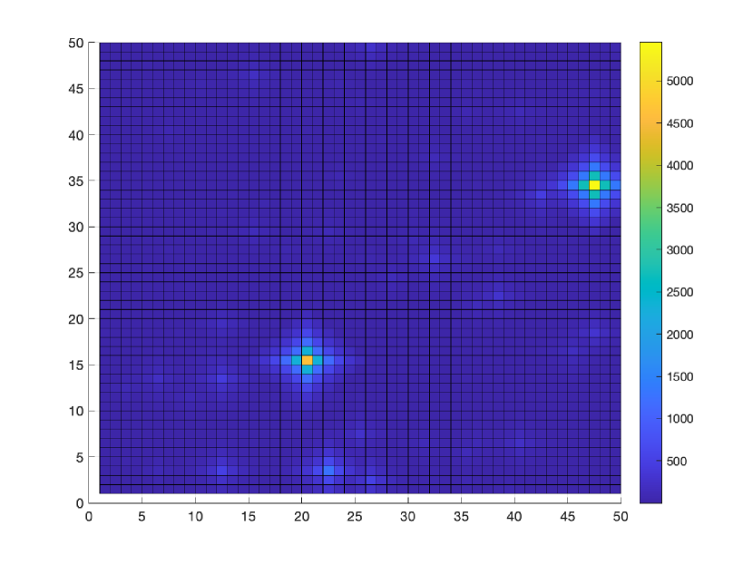
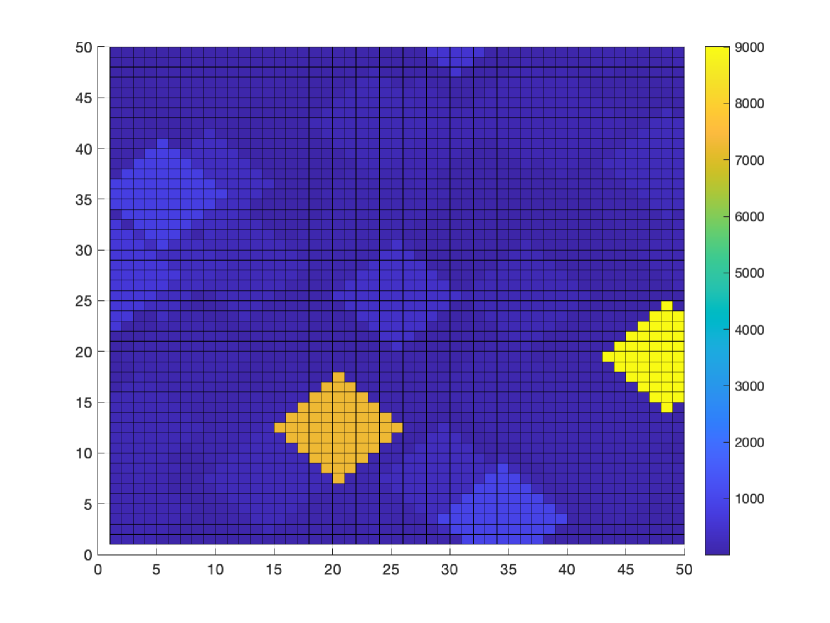
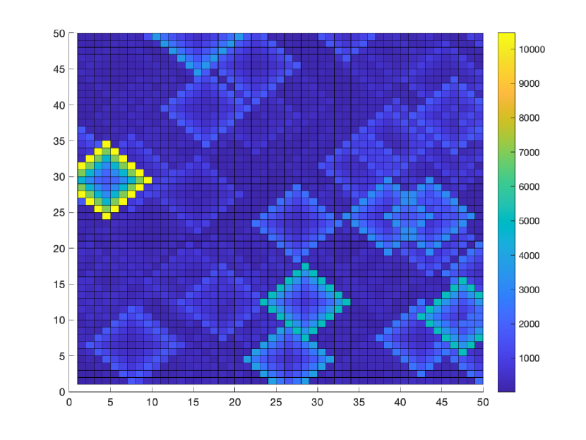
Figure 1. Simulated sample paths of the MMA random field on $\Lambda_{50}^{2}$ with weight function (6.1), $\phi=0.5$ (top left), $\phi=1.0$ (top right) and $\phi=1.5$ (bottom).

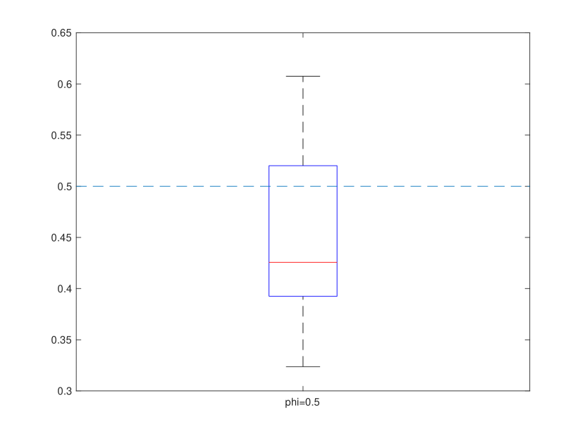
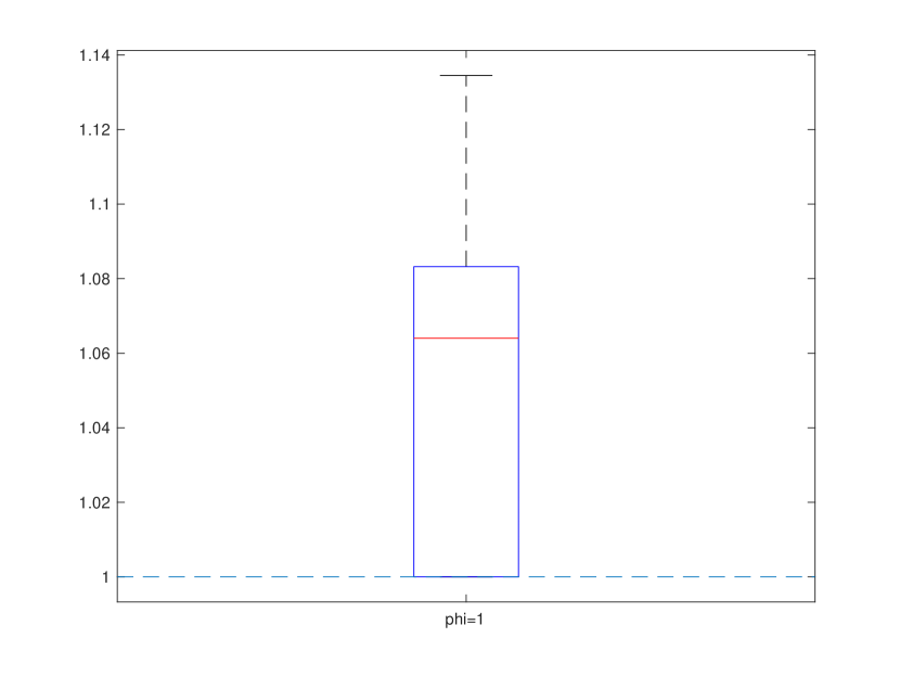
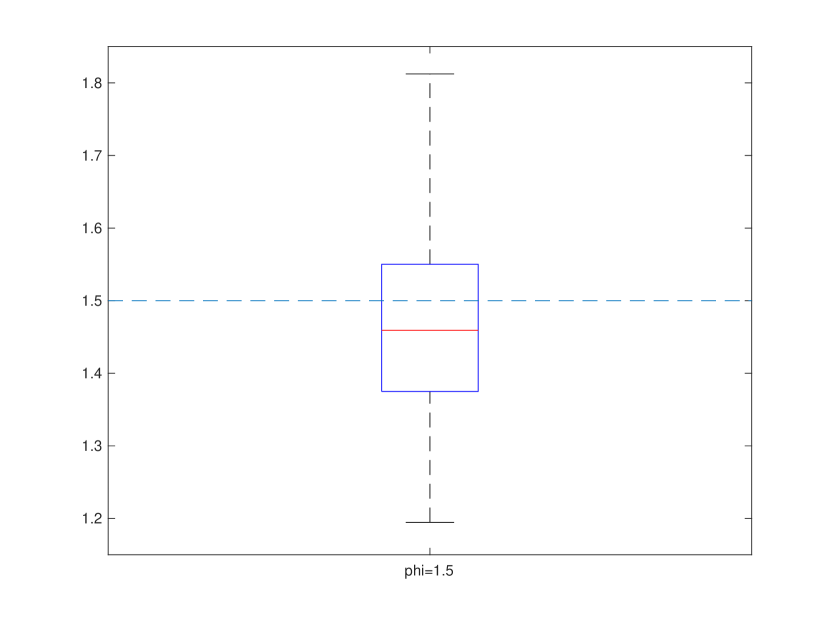
Figure 2. Box-plot (50 replications) for MMA Whittle estimation on $\Lambda_{50}^{2}$ of the parameter in model (6.1). $\phi=0.5$ (top left), $\phi=1.0$ (top right) and $\phi=1.5$ (bottom). $a_{m}$ represents the 95% empirical quantile.

6.2. The Brown-Resnick random field

In Figure 3 we present a simulation of the Brown-Resnick random field for $H=0.5$ on $\Lambda_{50}^{2}$. The simulation of these fields is complex; see the discussion in the recent overview paper Oesting and Strokorb [39]. For the results in Figure 3 and Table 1 we use the algorithm from Liu et al. [35] which leads to a perfect simulation of the field. For the field on $\Lambda_{50}^{2}$ we illustrate the performance of the Whittle estimator in boxplots based on 50 replications for $m_{n}=5,10$ corresponding to the 80%- and 90%-quantiles $a_{m}$ of the marginal distribution of the field. For these 50 sample paths we also calculated the pairwise composite likelihood estimator used in Davis et al. [15] and showed the results in a boxplot. Table 1 provides the mean, median, standard deviation based on 50 replications for the Whittle and pairwise composite likelihood estimators. The pairwise likelihood estimator has a much smaller variance than the Whittle estimator. On the other hand, pairwise likelihood estimation is very biased and costs much more time.

Figure 4 shows a simulation of a truncated Brown-Resnick random field for $H=0.5$ based on the naive approximation

(6.2) $$X_{{\bf s}}=\sup_{1\leq j\leq 1000}\Gamma_{j}^{-1}{\rm e}\,^{W_{{\bf s}}^{(j)}-\delta({\bf s})}\,,\quad{\bf s}\in\Lambda_{20}^{2}\,,$$

where $(\Gamma_{j})$ is defined in (3.1) which is independent of the sequence of iid standard Brownian sheets $(W_{{\bf s}}^{(j)})_{{\bf s}\in\Lambda_{20}^{2}}$. The performance of the Whittle estimator is illustrated in boxplots based on $50$ replications for $m_{n}=3,5$ corresponding to the $67\%$- and $80\%$-quantiles $a_{m}$ of the marginal distribution of the field. Perhaps surprisingly, according to Table 2, the choice of $m_{n}=3$ provides better estimation results with smaller bias and variance. For the same sample paths of the field we calculated the pairwise composite likelihood estimator. The boxplot in Figure 4 but also the results about mean, median, standard deviation in Table 2 indicate that the Whittle estimator outperforms pairwise likelihood; the Whittle procedure leads to estimators with smaller bias and variance.

Tables 1 and 2 show that the Whittle estimator can be calculated at a much faster average speed than the pairwise likelihood estimator. Moreover, the median of Whittle estimation is much closer to the true value $H=0.5$ than for pairwise likelihood, showing that the former estimator is less biased.

A delicate problem is the choice of a high quantile $a_{m}$. In our simulations we calculated it as the corresponding empirical $(1-1/m)$-quantile. Then we determined the spatial periodogram based on the indicator functions ${\bf 1}(|X_{{\bf s}}|>a_{m})$, ${\bf s}\in\Lambda_{n}^{2}$, and obtained the corresponding Whittle estimator by solving the optimization problem (4.1). Throughout the paper we use the function fminbnd in Matlab 2020a for optimization problems, also for pairwise likelihood.

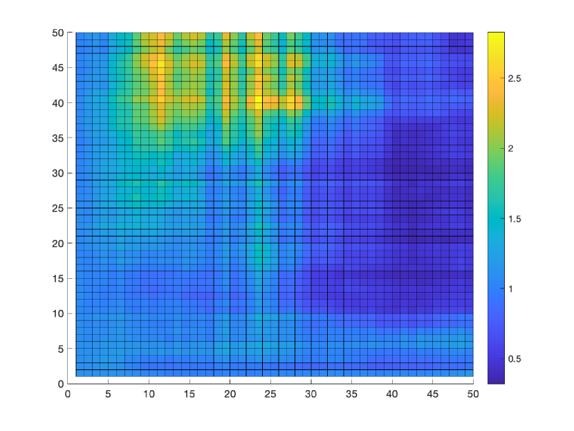
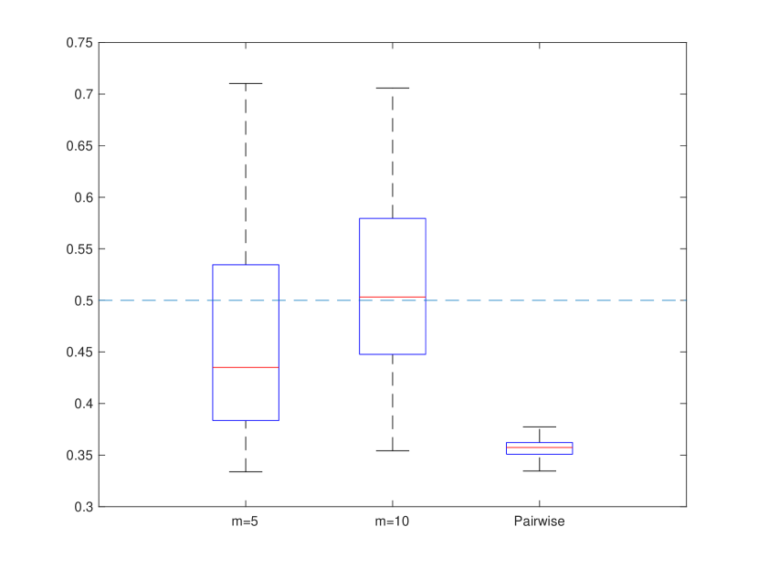
Figure 3. Left: A sample path of the Brown-Resnick random field on $\Lambda_{50}^{2}$ with $H=0.5$. The simulation is based on the algorithm from Liu et al. [35]. Right: Boxplots based on 50 replications of the Whittle estimator with $m_{n}=5,10$ and pairwise likelihood estimator; see [15] for details.

Estimator	Mean	Median	Standard Deviation	Time cost (seconds)
Whittle ($m=5$)	0.49	0.43	0.15	319
Whittle ($m=10$)	0.55	0.50	0.16	323
Pairwise	0.36	0.36	0.01	3205

Table 1. Mean, median, standard deviation and average time cost in seconds for the Whittle estimator (first and second row) and the pairwise composite likelihood estimator (third row). The estimation (50 replications) was conducted on a MacBook Pro (16-inch, 2019), CPU Intel Core i9 (2.4GHz) with Matlab 2020a.

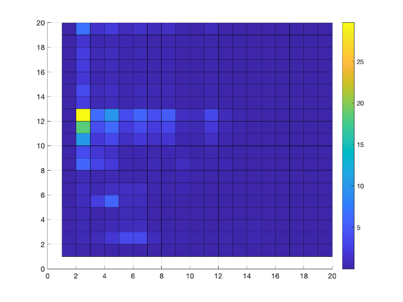
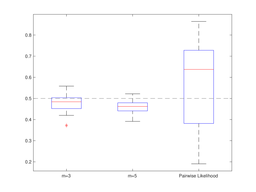
Figure 4. Left: A sample path of the approximation (6.2) to the Brown-Resnick random field on $\Lambda_{20}^{2}$ with $H=0.5$. Right: Boxplot based on 50 replications for Whittle estimator with $m_{n}=3,5$ and pairwise likelihood estimator; see [15] for details.

Estimator	Mean	Median	Standard Deviation	Time cost (seconds)
Whittle ($m=3$)	0.47	0.48	0.037	146
Whittle ($m=5$)	0.46	0.46	0.027	160
Pairwise	0.57	0.63	0.19	7946

Table 2. Mean, median, standard deviation and average time cost in seconds for Whittle estimator (first and second row) and pairwise composite likelihood estimator (third row). The estimation (50 replications) was conducted on a MacBook Pro (16-inch, 2019), CPU Intel Core i9 (2.4GHz) with Matlab 2020a.

6.3. Comments

Several problems are not discussed in detail here. One is the choice of the high quantile $a_{m}$ when dealing with real-life data. Davis et al. [16, 17] recommend a graphical approach by plotting the sample extremogram for various high empirical quantiles of the data at different lags. If the sample extremogram collapses into zero already at small lags this is an indication of the fact that $a_{m}$ has been chosen too high. Often 95%–97% quantiles of the data yield good results provided the sample size is sufficiently large. In our simulation study we did not choose very high quantiles and still got reasonable results. This may be due to the fact that the tails of the considered processes are almost exact power laws even for small arguments.

In the literature, estimation for Brown-Resnick processes/fields is often conducted for processes with a spatio-temporal structure. An extension of our results to these processes/fields is not straightforward since we need positivity of the spectral density on the parameter space. For example, Theorem 5.1 yields the positivity of the spectral density $f_{H}$ of the Brown-Resnick process; the proof heavily depends on the isotropy of the process.

Another reason why we find it difficult to compare our results with the literature on estimation of the Brown-Resnick process/field is the use of distinct simulation procedures. Often the naive approximation (6.2) is employed, or the simulation technique is not explicitly mentioned. Oesting and Strokorb [39] give an overview on simulation techniques for max-stable processes and point at various problems in this context, in particular when using (6.2).

One of the tasks to be solved in the future is to find confidence bands tailored for Whittle estimation. Motivated by results in Davis et al. [17, 13] for the estimation of the extremogram we expect that stationary and multiplier block bootstrap techniques may be suitable in this context.

7. Proof of Theorem 2.6

Write

$$\psi_{{\bf h}}^{(n)}=\frac{(2\pi)^{2}}{n^{2}}\sum_{{\bf j}\in\Lambda_{n}^{2}}\cos({\bf h}^{\top}\mbox{\boldmath$\lambda$}_{{\bf j}})\,g(\mbox{\boldmath$\lambda$}_{{\bf j}})\quad\mbox{ and }\quad\psi_{\bf h}=\int_{\Pi^{2}}\cos({\bf h}^{\top}\mbox{\boldmath$\omega$})g(\mbox{\boldmath$\omega$})\mathop{}\!\mathrm{d}\mbox{\boldmath$\omega$}\,.$$

Then we have

$$\dfrac{(2\pi)^{2}}{n^{2}}\sum_{{\bf j}\in\Lambda_{n}^{2}}(\widehat{f}(\mbox{\boldmath$\lambda$}_{\bf j})-f(\mbox{\boldmath$\lambda$}_{\bf j}))\,g(\mbox{\boldmath$\lambda$}_{\bf j}) = \sum_{\|{\bf h}\|<n}\psi_{\bf h}^{(n)}(\widehat{\gamma}({\bf h})-\gamma({\bf h}))$$

Since $g$ is continuous on $\Pi^{2}$ we have for fixed ${\bf h}$, $\psi_{\bf h}^{(n)}\to\psi_{\bf h}$ and $\sup_{{\bf h}}|\psi_{\bf h}^{(n)}|<\infty$. Then by virtue of Theorem 2.3,

$$\frac{n}{\sqrt{m_{n}}}\sum_{{\bf h}:\|{\bf h}\|\leq h}\psi_{\bf h}^{(n)}(\widehat{\gamma}({\bf h})-\gamma({\bf h}))\stackrel{{\scriptstyle d}}{{\rightarrow}}\sum_{{\bf h}:\|{\bf h}\|\leq h}\psi_{\bf h}\,Z_{\bf h}\,,\qquad n\to\infty\,.$$

We will show that for all $\varepsilon>0$,

(7.1) $$\lim_{h\to\infty}\limsup_{n\to\infty}{\mathbb{P}}\Big{(}\frac{n}{\sqrt{m_{n}}}\Big{|}\sum_{h<\|{\bf h}\|<n}\psi_{{\bf h}}^{(n)}(\widehat{\gamma}({\bf h})-\gamma({\bf h}))\Big{|}>\varepsilon\Big{)}=0\,.$$

Then, by Theorem 2 in Dehling et al. [20], it follows that

$$\dfrac{n}{\sqrt{m_{n}}}\,\dfrac{(2\pi)^{2}}{n^{2}}\sum_{{\bf j}\in\Lambda_{n}^{2}}(\widehat{f}(\mbox{\boldmath$\lambda$}_{\bf j})-f(\mbox{\boldmath$\lambda$}_{\bf j}))\,g(\mbox{\boldmath$\lambda$}_{\bf j})\stackrel{{\scriptstyle d}}{{\rightarrow}}\sum_{{\bf h}\in{\mathbb{Z}}^{2}}\psi_{\bf h}\,Z_{\bf h}\,,\qquad n\to\infty\,,$$

and the limit is a genuine real-valued random variable.

It remains to prove the following result.

Lemma 7.1.

Under the conditions of the theorem we have

$$\lim_{h\to\infty}\limsup_{n\to\infty}\dfrac{n}{\sqrt{m_{n}}}\Big{|}\sum_{h<\|{\bf h}\|<n}\psi_{{\bf h}}^{(n)}({\mathbb{E}}[\widehat{\gamma}({\bf h})]-\gamma({\bf h}))\Big{|} = 0\,.$$

Proof of Lemma 7.1.

By Lemma A.1 we have $|\psi_{{\bf h}}^{(n)}-\psi_{\bf h}|\leq cn^{-1}$ for $h_{1},h_{2}\leq n/2$. Hence

$$\dfrac{n}{\sqrt{m_{n}}}\,\Big{|}\sum_{h<\|{\bf h}\|\leq r_{n}}\psi_{{\bf h}}^{(n)}\,({\mathbb{E}}[\widehat{\gamma}({\bf h})]-\gamma({\bf h}))\Big{|}$$

$$\leq \dfrac{n}{\sqrt{m_{n}}}\,\Big{|}\sum_{h<\|{\bf h}\|\leq r_{n}}(\psi_{{\bf h}}^{(n)}-\psi_{\bf h})\,({\mathbb{E}}[\widehat{\gamma}({\bf h})]-\gamma({\bf h}))\Big{|}+\dfrac{n}{\sqrt{m_{n}}}\,\Big{|}\sum_{h<\|{\bf h}\|\leq r_{n}}\psi_{\bf h}\,({\mathbb{E}}[\widehat{\gamma}({\bf h})]-\gamma({\bf h}))\Big{|}$$

$$\leq \dfrac{r_{n}^{2}}{\sqrt{m_{n}}}\,c\,\sup_{h<\|{\bf h}\|\leq r_{n}}|{\mathbb{E}}[\widehat{\gamma}({\bf h})]-\gamma({\bf h})|+\sum_{h<\|{\bf h}\|\leq r_{n}}|\psi_{\bf h}|\,\dfrac{n}{\sqrt{m_{n}}}\sup_{h<\|{\bf h}\|\leq r_{n}}\big{|}{\mathbb{E}}[\widehat{\gamma}({\bf h})]-\gamma({\bf h})\big{|}\,.$$

The right-hand side vanishes as $n\to\infty$ in view of (M2) and the absolute summability of $(\psi_{\bf h})$. Next we consider

$$\dfrac{n}{\sqrt{m_{n}}}\,\Big{|}\sum_{r_{n}<\|{\bf h}\|<n}\psi_{{\bf h}}^{(n)}\,({\mathbb{E}}[\widehat{\gamma}({\bf h})]-\gamma({\bf h}))\Big{|}$$

$$\leq \dfrac{n}{\sqrt{m_{n}}}\,c\,\sum_{r_{n}<\|{\bf h}\|<n}|\psi_{{\bf h}}^{(n)}|\,\big{(}m_{n}\,|{\mathbb{P}}(|X_{\bf 0}|>a_{m}\,,|X_{\bf h}|>a_{m})-({\mathbb{P}}(|X|>a_{m}))^{2}|+\gamma({\bf h})\big{)}$$

$$\leq n\,m_{n}^{1/2}\,c\,\sum_{r_{n}<\|{\bf h}\|<n}\alpha(\|{\bf h}\|)+\dfrac{n}{\sqrt{m_{n}}}c\,\sum_{r_{n}<\|{\bf h}\|<n}\gamma({\bf h})$$

$$\leq n\,m_{n}^{1/2}\,c\,\alpha(r_{n})+\dfrac{n}{\sqrt{m_{n}}}c\,\sum_{r_{n}<\|{\bf h}\|<n}\gamma({\bf h})\to 0\,,\qquad n\to\infty\,.$$

In the last step we used condition (2.10). This finishes the proof. ∎

By virtue of Lemma 7.1 we are allowed to replace all $\gamma({\bf h})$ in (7.1) by the corresponding expectations ${\mathbb{E}}[\widehat{\gamma}({\bf h})]$. Therefore we will show next that the following quantities are asymptotically negligible for all fixed $\varepsilon>0$:

$$Q_{1} = {\mathbb{P}}\Big{(}\frac{n}{\sqrt{m_{n}}}\Big{|}\sum_{{\bf h}:h<\|{\bf h}\|\leq 3r_{n}}\psi_{{\bf h}}^{(n)}(\widehat{\gamma}({\bf h})-{\mathbb{E}}[\widehat{\gamma}({\bf h})])\Big{|}>\varepsilon\Big{)}\,,$$

$$Q_{2} = {\mathbb{P}}\Big{(}\frac{n}{\sqrt{m_{n}}}\Big{|}\sum_{{\bf h}:3r_{n}<\|{\bf h}\|\leq n}\psi_{{\bf h}}^{(n)}(\widehat{\gamma}({\bf h})-{\mathbb{E}}[\widehat{\gamma}({\bf h})])\Big{|}>\varepsilon\Big{)}\,.$$

By Markov’s inequality and Lemma A.1,3., also using the fact that $r_{n}\leq n/2$, we have

$$Q_{1} \leq \dfrac{2\,n}{\sqrt{m_{n}}}\sum_{{\bf h}:h<\|{\bf h}\|\leq 3r_{n}}|\psi_{\bf h}^{(n)}|\,{\mathbb{E}}[|\widehat{\gamma}({\bf h})|]$$

$$\leq c\,\sqrt{m_{n}}\,\sum_{{\bf h}:h<\|{\bf h}\|\leq 3r_{n}}\big{(}{\mathbb{P}}(|X_{\bf 0}|>a_{m}\,,|X_{\bf h}|>a_{m})+({\mathbb{P}}(|X|>a_{m}))^{2}\big{)}$$

$$= c\,\sqrt{m_{n}}\,\sum_{{\bf h}:h<\|{\bf h}\|\leq 3r_{n}}{\mathbb{P}}(|X_{\bf 0}|>a_{m}\,,|X_{\bf h}|>a_{m})+O(r_{n}^{2}m_{n}^{-3/2})\,.$$

The right-hand side vanishes by condition (M1), first letting $n\to\infty$, then $h\to\infty$.

The negligibility of $Q_{2}$ is proved in the following lemma. Its proof is given in Appendix B.

Lemma 7.2.

Under the conditions of the theorem we have $\lim_{n\to\infty}Q_{2}=0$.

This completes the proof.

8. Proof of Theorem 4.2

We start with several auxiliary results.

Lemma 8.1.

Assume (W). Then the following statements hold:

1. For all $\Theta\in\mbox{\boldmath$\Theta$}$, $\Theta\neq\Theta_{0}$,

   (8.1) $$\dfrac{1}{(2\pi)^{2}}\dfrac{\overline{\sigma}^{2}(\Theta)}{\overline{\sigma}^{2}(\Theta_{0})}\,\int_{\Pi^{2}}\frac{f_{\Theta_{0}}(\mbox{\boldmath$\omega$})}{f_{\Theta}(\mbox{\boldmath$\omega$})}\mathop{}\!\mathrm{d}\mbox{\boldmath$\omega$}>1\,,\mbox{ where }\overline{\sigma}^{2}(\Theta)=\exp\Big{(}\dfrac{1}{(2\pi)^{2}}\int_{\Pi^{2}}\log f_{\Theta}(\mbox{\boldmath$\omega$})\,d\mbox{\boldmath$\omega$}\Big{)}\,.$$

2. We have

   $$\sup_{\Theta\in\mbox{\boldmath$\Theta$}}\Big{|}\sigma_{n}^{2}(\Theta)-\dfrac{\overline{\sigma}^{2}(\Theta)}{(2\pi)^{2}}\int_{\Pi^{2}}\dfrac{f_{\Theta_{0}}(\mbox{\boldmath$\omega$})}{f_{\Theta}(\mbox{\boldmath$\omega$})}\,d\mbox{\boldmath$\omega$}\Big{|}\to 0\,,\qquad n\to\infty\,.$$

3. We have $\Theta_{n}\stackrel{{\scriptstyle{\mathbb{P}}}}{{\rightarrow}}\Theta_{0}$ and $\sigma_{n}^{2}(\Theta_{n})\stackrel{{\scriptstyle{\mathbb{P}}}}{{\rightarrow}}\overline{\sigma}^{2}(\Theta_{0})$.

The proof is given at the end of this section.

Part 1. says that the left-hand side of (8.1) is bounded away from 1. This fact is essentially responsible for the uniqueness of the Whittle estimator. Part 2. is key to showing the asymptotic unbiasedness of the Whittle estimator. Part 3. yields the consistency of the Whittle estimator.

Proof of Theorem 4.2.

Let

(8.2) $$F_{n}(\mbox{\boldmath$\omega$},\Theta)=\dfrac{f_{\Theta}(\mbox{\boldmath$\omega$})}{\overline{\sigma}_{n}^{2}(\Theta)}\quad\mbox{and}\quad F(\mbox{\boldmath$\omega$},\Theta)=\dfrac{f_{\Theta}(\mbox{\boldmath$\omega$})}{\overline{\sigma}^{2}(\Theta)}\,,\qquad(\mbox{\boldmath$\omega$},\Theta)\in\Pi^{2}\times\mbox{\boldmath$\Theta$}\,.$$

By Kolmogorov’s formula (see Brockwell and Davis [8], Theorem 5.8.1),

(8.3) $$\sum_{{\bf j}\in\Lambda_{n}^{2}}\log F_{n}(\mbox{\boldmath$\lambda$}_{{\bf j}},\Theta)=\int_{\Pi^{2}}\log F(\mbox{\boldmath$\omega$},\Theta)\mathop{}\!\mathrm{d}\mbox{\boldmath$\omega$}=0\,,\quad\Theta\in\mbox{\boldmath$\Theta$}\,.$$

We further study the expressions of $\partial F_{n}(\mbox{\boldmath$\omega$},\Theta)/\partial\theta_{s_{1}}$ and $\partial^{2}F_{n}(\mbox{\boldmath$\omega$},\Theta)/(\partial\theta_{s_{1}}\partial\theta_{s_{2}})$ for $s_{i}\in\{1,\ldots,s\}$.

$$\frac{\partial F_{n}(\mbox{\boldmath$\omega$},\Theta)}{\partial\theta_{s_{1}}} = \dfrac{1}{\overline{\sigma}_{n}^{2}(\Theta)}\frac{\partial f_{\Theta}(\mbox{\boldmath$\omega$})}{\partial\theta_{s_{1}}}-\frac{f_{\Theta}(\mbox{\boldmath$\omega$})}{(\overline{\sigma}^{2}(\Theta))^{2}}\frac{\partial\overline{\sigma}_{n}^{2}(\Theta)}{\partial\theta_{s_{1}}}$$

$$= \frac{1}{\overline{\sigma}_{n}^{2}(\Theta)}\frac{\partial f_{\Theta}(\mbox{\boldmath$\omega$})}{\partial\theta_{s_{1}}}-\frac{f_{\Theta}(\mbox{\boldmath$\omega$})}{\overline{\sigma}_{n}^{2}(\Theta)}\Big{(}n^{-2}\sum_{{\bf j}\in\Lambda_{n}}(f_{\Theta}(\lambda_{{\bf j}}))^{-1}\frac{\partial f_{\Theta}(\lambda_{{\bf j}})}{\partial\theta_{s_{1}}}\Big{)}\,.$$

$$\frac{\partial^{2}F_{n}(\mbox{\boldmath$\omega$},\Theta)}{\partial\theta_{s_{1}}\partial\theta_{s_{2}}} = \frac{1}{\overline{\sigma}_{n}^{2}(\Theta)}\frac{\partial^{2}f_{\Theta}(\mbox{\boldmath$\omega$})}{\partial\theta_{s_{1}}\partial\theta_{s_{2}}}-(\overline{\sigma}_{n}^{2}(\Theta))^{-1}\frac{\partial f_{\Theta}(\mbox{\boldmath$\omega$})}{\partial\theta_{s_{1}}}\Big{(}n^{-2}\sum_{{\bf j}\in\Lambda_{n}}(f_{\Theta}(\lambda_{{\bf j}}))^{-1}\frac{\partial f_{\Theta}(\lambda_{{\bf j}})}{\partial\theta_{s_{2}}}\Big{)}$$

$$+\frac{f_{\Theta}(\mbox{\boldmath$\omega$})}{\overline{\sigma}_{n}^{2}(\Theta)}\Big{(}n^{-2}\sum_{{\bf j}\in\Lambda_{n}}(f_{\Theta}(\lambda_{{\bf j}}))^{-1}\frac{\partial f_{\Theta}(\lambda_{{\bf j}})}{\partial\theta_{s_{1}}}\Big{)}\Big{(}n^{-2}\sum_{{\bf j}\in\Lambda_{n}}(f_{\Theta}(\lambda_{{\bf j}}))^{-1}\frac{\partial f_{\Theta}(\lambda_{{\bf j}})}{\partial\theta_{s_{2}}}\Big{)}$$

$$+\frac{f_{\Theta}(\mbox{\boldmath$\omega$})}{\overline{\sigma}_{n}^{2}(\Theta)}\Big{(}n^{-2}\sum_{{\bf j}\in\Lambda_{n}}(f_{\Theta}(\lambda_{{\bf j}}))^{-1}\frac{\partial^{2}f_{\Theta}(\lambda_{{\bf j}})}{\partial\theta_{s_{1}}\partial\theta_{s_{2}}}\Big{)}\,.$$

In view of (4.3), (4.4) the first- and second-order derivatives of $F_{n}(\mbox{\boldmath$\omega$},\Theta)$ and $F(\mbox{\boldmath$\omega$},\Theta)$ with respect to $\Theta$ exist. Moreover, (4.5) implies that $\overline{\sigma}^{2}(\Theta)$ and $\overline{\sigma}_{n}^{2}(\Theta)$ are uniformly bounded in $\Theta$ and thus both $F_{n}(\mbox{\boldmath$\omega$},\Theta)$, $F(\mbox{\boldmath$\omega$},\Theta)$ are bounded away from zero uniformly for $(\mbox{\boldmath$\omega$},\Theta)\in\Pi^{2}\times\mbox{\boldmath$\Theta$}$. Consequently, the first- and second-order derivatives of $1/F_{n}(\mbox{\boldmath$\omega$},\Theta)$ and $1/F(\mbox{\boldmath$\omega$},\Theta)$ are well defined. Taking the derivatives of both terms in (8.3), we have

$${\bf 0}_{1\times s} = \sum_{{\bf j}\in\Lambda_{n}^{2}}\frac{\partial F_{n}(\mbox{\boldmath$\lambda$}_{{\bf j}},\Theta)}{\partial\Theta}\frac{1}{F_{n}(\mbox{\boldmath$\lambda$}_{{\bf j}},\Theta)}=\sum_{{\bf j}\in\Lambda_{n}^{2}}f_{\Theta}(\mbox{\boldmath$\lambda$}_{{\bf j}})\frac{\partial(1/F_{n}(\mbox{\boldmath$\lambda$}_{{\bf j}},\Theta))}{\partial\Theta}$$

$$= \int_{\Pi^{2}}\dfrac{1}{F(\mbox{\boldmath$\omega$},\Theta)}\frac{\partial F(\mbox{\boldmath$\omega$},\Theta)}{\partial\Theta}\mathop{}\!\mathrm{d}\mbox{\boldmath$\omega$}=\int_{\Pi^{2}}f_{\Theta}(\mbox{\boldmath$\omega$})\frac{\partial(1/F(\mbox{\boldmath$\omega$},\Theta))}{\partial\Theta}\mathop{}\!\mathrm{d}\mbox{\boldmath$\omega$}\,,$$

$${\bf 0}_{s\times s} = \sum_{{\bf j}\in\Lambda_{n}^{2}}\dfrac{1}{F_{n}(\mbox{\boldmath$\lambda$}_{{\bf j}},\Theta)}\frac{\partial^{2}F_{n}(\mbox{\boldmath$\lambda$}_{{\bf j}},\Theta)}{\partial\Theta^{2}}-\sum_{{\bf j}\in\Lambda_{n}^{2}}\bigg{(}\dfrac{1}{F_{n}(\mbox{\boldmath$\lambda$}_{{\bf j}},\Theta)}\frac{\partial F_{n}(\mbox{\boldmath$\lambda$}_{{\bf j}},\Theta)}{\partial\Theta}\bigg{)}^{\top}\bigg{(}\dfrac{1}{F_{n}(\mbox{\boldmath$\lambda$}_{{\bf j}},\Theta)}\frac{\partial F_{n}(\mbox{\boldmath$\lambda$}_{{\bf j}},\Theta)}{\partial\Theta}\bigg{)}$$

$$= \sum_{{\bf j}\in\Lambda^{2}}\dfrac{1}{F_{n}(\mbox{\boldmath$\lambda$}_{{\bf j}},\Theta)}\frac{\partial^{2}F_{n}(\mbox{\boldmath$\lambda$}_{{\bf j}},\Theta)}{\partial\Theta^{2}}-\sum_{{\bf j}\in\Lambda_{n}^{2}}\bigg{(}\frac{\partial\log F_{n}(\mbox{\boldmath$\lambda$}_{{\bf j}},\Theta)}{\partial\Theta}\bigg{)}^{\top}\bigg{(}\frac{\partial\log F_{n}(\mbox{\boldmath$\lambda$}_{{\bf j}},\Theta)}{\partial\Theta}\bigg{)}$$

$$= \int_{\Pi^{2}}\dfrac{1}{F(\mbox{\boldmath$\omega$},\Theta)}\frac{\partial^{2}F(\mbox{\boldmath$\omega$},\Theta)}{\partial\Theta^{2}}\mathop{}\!\mathrm{d}\mbox{\boldmath$\omega$}-\int_{\Pi^{2}}\bigg{(}\frac{\partial\log F(\mbox{\boldmath$\omega$},\Theta)}{\partial\Theta}\bigg{)}^{\top}\bigg{(}\frac{\partial\log F(\mbox{\boldmath$\omega$},\Theta)}{\partial\Theta}\bigg{)}\mathop{}\!\mathrm{d}\mbox{\boldmath$\omega$}\,.$$

By definition of the Whittle estimator $\Theta_{n}$ as a minimizer, $\partial\sigma_{n}^{2}(\Theta_{n})/\partial\Theta={\bf 0}_{1\times s}$. Then a Taylor expansion of $\partial\sigma^{2}_{n}(\Theta)/\partial\Theta$ about $\Theta=\Theta_{n}$ yields

(8.6) $$\frac{\partial\sigma^{2}_{n}(\Theta_{0})}{\partial\Theta} = \frac{\partial\sigma^{2}_{n}(\Theta_{n})}{\partial\Theta}-\frac{\partial^{2}\sigma^{2}_{n}(\Theta_{n}^{+})}{\partial\Theta^{2}}\big{(}\Theta_{n}-\Theta_{0}\big{)}=-\frac{\partial^{2}\sigma^{2}_{n}(\Theta_{n}^{+})}{\partial\Theta^{2}}\big{(}\Theta_{n}-\Theta_{0}\big{)}\,,$$

for some $\Theta_{n}^{+}\in\mbox{\boldmath$\Theta$}$ with $\Theta_{n}^{+}\stackrel{{\scriptstyle{\mathbb{P}}}}{{\rightarrow}}\Theta_{0}$; see Lemma 8.1,3. By Lemma 8.2 and (LABEL:eq:zeros001) we have

$$\frac{\partial^{2}\sigma^{2}_{n}(\Theta_{n}^{+})}{\partial\Theta^{2}} \stackrel{{\scriptstyle{\mathbb{P}}}}{{\rightarrow}} \frac{\overline{\sigma}^{2}(\Theta_{0})}{(2\pi)^{2}}\int_{\Pi^{2}}\dfrac{1}{F(\mbox{\boldmath$\omega$},\Theta_{0})}\frac{\partial^{2}F(\mbox{\boldmath$\omega$},\Theta_{0})}{\partial\Theta^{2}}\mathop{}\!\mathrm{d}\mbox{\boldmath$\omega$}$$

$$= \frac{\overline{\sigma}^{2}(\Theta_{0})}{(2\pi)^{2}}\int_{\Pi^{2}}\bigg{(}\frac{\partial\log F(\mbox{\boldmath$\omega$},\Theta_{0})}{\partial\Theta}\bigg{)}^{\top}\bigg{(}\frac{\partial\log F(\mbox{\boldmath$\omega$},\Theta_{0})}{\partial\Theta}\bigg{)}\mathop{}\!\mathrm{d}\mbox{\boldmath$\omega$}=:\frac{\overline{\sigma}^{2}(\Theta_{0})}{(2\pi)^{2}}\widehat{W}\,.$$

In fact, we have for ${\bf U}$ uniform on $\Pi^{2}$,

$$\dfrac{\widehat{W}}{(2\pi)^{2}} = \dfrac{1}{(2\pi)^{2}}\int_{\Pi^{2}}\Big{[}\Big{(}\frac{\partial\log f_{\Theta_{0}}(\mbox{\boldmath$\omega$})}{\partial\Theta}-\frac{1}{(2\pi)^{2}}\int_{\Pi^{2}}\frac{\partial\log f_{\Theta_{0}}(\mbox{\boldmath$\omega$})}{\partial\Theta}\mathop{}\!\mathrm{d}\mbox{\boldmath$\omega$}\Big{)}^{\top}$$

$$\hskip 22.76228pt\Big{(}\frac{\partial\log f_{\Theta_{0}}(\mbox{\boldmath$\omega$})}{\partial\Theta}-\frac{1}{(2\pi)^{2}}\int_{\Pi^{2}}\frac{\partial\log f_{\Theta_{0}}(\mbox{\boldmath$\omega$})}{\partial\Theta}\mathop{}\!\mathrm{d}\mbox{\boldmath$\omega$}\Big{)}\Big{]}{\rm d}\mbox{\boldmath$\lambda$}$$

$$= {\rm var}\Big{(}\frac{\partial\log f_{\Theta_{0}}({\bf U})}{\partial\Theta}\Big{)}\,.$$

By condition (W), $\widehat{W}$ is non-singular. Together with (8) this implies that $\partial^{2}\sigma^{2}_{n}(\Theta_{n}^{+})/\partial\Theta^{2}$ is positive definite on a set $B_{n}$ with ${\mathbb{P}}(B_{n})\to 1$. The definition of the Whittle likelihood $\sigma^{2}_{n}(\Theta)$ and (LABEL:eq:zeros000) yield

$$\frac{\partial\sigma^{2}_{n}(\Theta_{0})}{\partial\Theta}=\sum_{{\bf j}\in\Lambda_{n}^{2}}\frac{\partial(1/F_{n}(\mbox{\boldmath$\lambda$}_{{\bf j}},\Theta_{0}))}{\partial\Theta}\,\widehat{f}(\mbox{\boldmath$\lambda$}_{{\bf j}})=\sum_{{\bf j}\in\Lambda_{n}^{2}}\frac{\partial(1/F_{n}(\mbox{\boldmath$\lambda$}_{{\bf j}},\Theta_{0}))}{\partial\Theta}\big{(}\widehat{f}(\mbox{\boldmath$\lambda$}_{{\bf j}})-f_{\Theta_{0}}(\mbox{\boldmath$\lambda$}_{{\bf j}})\big{)}\,.$$

Combining this relation with (8.6), we have

$$\frac{n}{\sqrt{m_{n}}}(\Theta_{n}-\Theta_{0}) = -\bigg{(}\frac{\partial^{2}\sigma_{n}^{2}(\Theta_{n}^{+})}{\partial\Theta^{2}}\bigg{)}^{-1}\frac{n}{\sqrt{m_{n}}}\sum_{{\bf j}\in\Lambda_{n}^{2}}\dfrac{1}{F^{2}_{n}(\mbox{\boldmath$\lambda$}_{{\bf j}},\Theta_{0})}\frac{\partial F_{n}(\mbox{\boldmath$\lambda$}_{{\bf j}},\Theta_{0})}{\partial\Theta}\big{(}\widehat{f}(\mbox{\boldmath$\lambda$}_{{\bf j}})-f_{\Theta_{0}}(\mbox{\boldmath$\lambda$}_{{\bf j}})\big{)}$$

$$= -\widehat{W}^{-1}\dfrac{(2\pi)^{2}}{\overline{\sigma}^{2}(\Theta_{0})}(1+o_{\mathbb{P}}(1))$$

$$\times\frac{n}{\sqrt{m_{n}}}\sum_{{\bf j}\in\Lambda_{n}^{2}}\dfrac{1}{F_{n}^{2}(\mbox{\boldmath$\lambda$}_{{\bf j}},\Theta_{0})}\frac{\partial F_{n}(\mbox{\boldmath$\lambda$}_{{\bf j}},\Theta_{0})}{\partial\Theta}\big{(}\widehat{f}(\mbox{\boldmath$\lambda$}_{{\bf j}})-f_{\Theta_{0}}(\mbox{\boldmath$\lambda$}_{{\bf j}})\big{)}\,.$$

Then, uniformly for $\mbox{\boldmath$\omega$}\in\Pi^{2}$,

$$\frac{\partial F_{n}(\mbox{\boldmath$\omega$},\Theta_{0})}{\partial\Theta} = -\frac{f_{\Theta_{0}}(\mbox{\boldmath$\omega$})}{\big{(}\overline{\sigma}_{n}^{2}(\Theta_{0})\big{)}^{2}}\frac{\partial\overline{\sigma}_{n}^{2}(\Theta_{0})}{\partial\Theta}=-\frac{f_{\Theta_{0}}(\mbox{\boldmath$\omega$})}{\overline{\sigma}_{n}^{2}(\Theta_{0})}\frac{\partial\log\overline{\sigma}_{n}^{2}(\Theta_{0})}{\partial\Theta}$$

$$= -\frac{f_{\Theta_{0}}(\mbox{\boldmath$\omega$})}{\overline{\sigma}_{n}^{2}(\Theta_{0})}\bigg{(}\frac{1}{n^{2}}\sum_{{\bf j}\in\Lambda_{n}^{2}}\dfrac{1}{f_{\Theta_{0}}(\mbox{\boldmath$\lambda$}_{{\bf j}})}\frac{\partial f_{\Theta_{0}}(\mbox{\boldmath$\lambda$}_{{\bf j}})}{\partial\Theta}\bigg{)}$$

$$= -\frac{f_{\Theta_{0}}(\mbox{\boldmath$\omega$})}{\overline{\sigma}^{2}(\Theta_{0})}\frac{1}{(2\pi)^{2}}\int_{\Pi^{2}}f^{-1}_{\Theta_{0}}(\mbox{\boldmath$\lambda$})\frac{\partial f_{\Theta_{0}}(\mbox{\boldmath$\lambda$})}{\partial\Theta}\,{\rm d}\mbox{\boldmath$\lambda$}(1+o(1))=:\frac{f_{\Theta_{0}}(\mbox{\boldmath$\omega$})}{\overline{\sigma}^{2}(\Theta_{0})}\,{\bf C}\,(1+o(1))\,.$$

Therefore, uniformly for $\omega$,

$$\dfrac{1}{F_{n}^{2}(\mbox{\boldmath$\omega$},\Theta_{0})}\frac{\partial F_{n}(\mbox{\boldmath$\omega$},\Theta_{0})}{\partial\Theta} = \frac{\overline{\sigma}^{2}(\Theta_{0})}{f_{\Theta_{0}}(\mbox{\boldmath$\omega$})}\,{\bf C}\,(1+o(1))\,,$$

and we finally have

$$\frac{n}{\sqrt{m_{n}}}(\Theta_{n}-\Theta_{0}) = -\widehat{W}^{-1}{\bf C}\,(2\pi)^{2}(1+o_{\mathbb{P}}(1))\frac{n}{\sqrt{m_{n}}}\sum_{{\bf j}\in\Lambda_{n}^{2}}\dfrac{\widehat{f}(\mbox{\boldmath$\lambda$}_{{\bf j}})-f_{\Theta_{0}}(\mbox{\boldmath$\lambda$}_{{\bf j}})}{f_{\Theta_{0}}(\mbox{\boldmath$\lambda$}_{\bf j})}\,.$$

The conditions of Theorem 2.6 are satisfied for $g=1/f_{\Theta_{0}}$. The second-order partial derivatives of $g({\bf x})$, ${\bf x}\in\Pi^{2}$, are given by

$$\frac{\partial^{2}g({\bf x})}{\partial x_{1}\partial x_{2}}=\frac{2}{f^{3}_{\Theta}({\bf x})}\frac{\partial f_{\Theta}({\bf x})}{\partial x_{1}}\frac{\partial f_{\Theta}({\bf x})}{\partial x_{2}}-\frac{1}{f^{2}_{\Theta}({\bf x})}\frac{\partial^{2}f_{\Theta}({\bf x})}{\partial x_{1}\partial x_{2}}\,.$$

Notice that $f_{\Theta_{0}}$ is bounded from below by (4.2), and due to (4.3) we have

(8.8) $$\Big{|}\frac{\partial f_{\Theta}({\bf x})}{\partial x_{1}}\frac{\partial f_{\Theta}({\bf x})}{\partial x_{2}}\Big{|}+\Big{|}\frac{\partial^{2}f_{\Theta}({\bf x})}{\partial x_{1}\partial x_{2}}\Big{|}\leq c\,\Big{(}\sum_{{\bf h}\in\mathbb{Z}^{2}}|h_{1}h_{2}\gamma_{\Theta}({\bf h})|\Big{)}^{2}<\infty\,,$$

Therefore, (2.11) is satisfied.

Now Theorem 2.6 yields

(8.9) $$\frac{n}{\sqrt{m_{n}}}(\Theta_{n}-\Theta_{0}) \stackrel{{\scriptstyle d}}{{\rightarrow}} -(2\pi)^{2}\,\Big{(}{\rm var}\Big{(}\dfrac{\partial\log f_{\Theta_{0}}({\bf U})}{\partial\Theta}\Big{)}\Big{)}^{-1}{\mathbb{E}}\Big{[}\dfrac{1}{f_{\Theta_{0}}({\bf U})}\frac{\partial f_{\Theta_{0}}({\bf U})}{\partial\Theta}\Big{]}$$

$$\times\sum_{{\bf h}\in{\mathbb{Z}}^{2}}Z_{h}\,\int_{\Pi^{2}}\cos({\bf h}^{\top}\mbox{\boldmath$\omega$})\,\dfrac{1}{f_{\Theta_{0}}(\mbox{\boldmath$\omega$})}\,{\rm d}\mbox{\boldmath$\omega$}=:{\bf G}\sim N({\bf 0},W)\,.$$

∎

Proof of Lemma 8.1

Part 1. We fix $\Theta\in\mbox{\boldmath$\Theta$}$. Condition (8.1) is satisfied if and only if $f_{\Theta_{0}}/f_{\Theta}$ is not a constant. Indeed, writing ${\bf U}$ for a uniform random vector on $\Pi^{2}$, (8.1) turns into

$$\exp\Big{(}-{\mathbb{E}}\Big{[}\log\dfrac{f_{\Theta_{0}}}{f_{\Theta}}({\bf U})\Big{]}\Big{)}{\mathbb{E}}\Big{[}\dfrac{f_{\Theta_{0}}}{f_{\Theta}}({\bf U})\Big{]}>1\,.$$

Taking logarithms, we get the equivalent inequality

$$\log\Big{(}{\mathbb{E}}\Big{[}\dfrac{f_{\Theta_{0}}}{f_{\Theta}}({\bf U})\Big{]}\Big{)}>{\mathbb{E}}\Big{[}\log\dfrac{f_{\Theta_{0}}}{f_{\Theta}}({\bf U})\Big{]}\,,$$

which is valid by Jensen’s inequality (8.1) with the exception that $f_{\Theta_{0}}/f_{\Theta}$ is constant.

Part 2. We have

$$\sup_{\Theta\in\mbox{\boldmath$\Theta$}}\Big{|}\sigma_{n}^{2}(\Theta)-\dfrac{\overline{\sigma}^{2}(\Theta)}{(2\pi)^{2}}\int_{\Pi^{2}}\dfrac{f_{\Theta_{0}}(\mbox{\boldmath$\omega$})}{f_{\Theta}(\mbox{\boldmath$\omega$})}\,d\mbox{\boldmath$\omega$}\Big{|}$$

$$\leq \sup_{\Theta\in\mbox{\boldmath$\Theta$}}\Big{|}\sigma_{n}^{2}(\Theta)-\dfrac{\overline{\sigma}^{2}(\Theta)}{n^{2}}\sum_{{\bf j}\in\Lambda_{n}^{2}}\dfrac{f_{\Theta_{0}}(\mbox{\boldmath$\lambda$}_{\bf j})}{f_{\Theta}(\mbox{\boldmath$\lambda$}_{\bf j})}\Big{|}+\sup_{\Theta\in\mbox{\boldmath$\Theta$}}\Big{|}\dfrac{\overline{\sigma}^{2}(\Theta)}{n^{2}}\sum_{{\bf j}\in\Lambda_{n}^{2}}\dfrac{f_{\Theta_{0}}(\mbox{\boldmath$\lambda$}_{\bf j})}{f_{\Theta}(\mbox{\boldmath$\lambda$}_{\bf j})}-\frac{\overline{\sigma}^{2}(\Theta)}{(2\pi)^{2}}\int_{\Pi^{2}}\dfrac{f_{\Theta_{0}}(\mbox{\boldmath$\omega$})}{f_{\Theta}(\mbox{\boldmath$\omega$})}\,d\mbox{\boldmath$\omega$}\Big{|}$$

$$=: J_{1}+J_{2}\,.$$

By uniform continuity of $(\overline{\sigma}^{2}(\Theta),f_{\Theta}(\mbox{\boldmath$\omega$}))$ on $\Pi^{2}\times\mbox{\boldmath$\Theta$}$, $\sup_{\Theta\in\mbox{\boldmath$\Theta$}}\overline{\sigma}^{2}(\Theta)<\infty$ and we have uniform convergence of the Riemann sums in $J_{2}$ to the limiting integrals. Therefore $J_{2}\to 0$. For the same reasons we also have $\sup_{\Theta\in\mbox{\boldmath$\Theta$}}|\overline{\sigma}_{n}^{2}(\Theta)-\overline{\sigma}^{2}(\Theta)|\to 0$. Now it suffices to show that

$$\widetilde{J}_{1} := \sup_{\Theta\in\mbox{\boldmath$\Theta$}}\Big{|}\dfrac{1}{n^{2}}\sum_{{\bf j}\in\Lambda_{n}^{2}}\dfrac{\widehat{f}(\mbox{\boldmath$\lambda$}_{\bf j})}{f_{\Theta}(\mbox{\boldmath$\lambda$}_{\bf j})}-\dfrac{1}{n^{2}}\sum_{{\bf j}\in\Lambda_{n}^{2}}\dfrac{f_{\Theta_{0}}(\mbox{\boldmath$\lambda$}_{\bf j})}{f_{\Theta}(\mbox{\boldmath$\lambda$}_{\bf j})}\Big{|}$$

$$= \sup_{\Theta\in\mbox{\boldmath$\Theta$}}\Big{|}\dfrac{1}{n^{2}}\sum_{{\bf j}\in\Lambda_{n}^{2}}\Big{(}\widehat{f}(\mbox{\boldmath$\lambda$}_{\bf j})-f_{\Theta_{0}}(\mbox{\boldmath$\lambda$}_{\bf j})\Big{)}\big{(}1/f_{\Theta}(\mbox{\boldmath$\lambda$}_{\bf j})\big{)}\Big{|}\,,$$

vanishes as $n\to\infty$. Let $q_{{\bf l}}(\mbox{\boldmath$\omega$};\Theta_{0})$ be the Cèsaro mean of the first ${\bf l}=(l,l)$-Fourier approximation to $1/f_{\Theta_{0}}$ on $\Pi^{2}$, i.e., for $\Theta\in\mbox{\boldmath$\Theta$}$,

$$q_{{\bf l}}(\mbox{\boldmath$\omega$};\Theta) = \frac{1}{l^{2}}\sum_{i_{1}=0}^{l-1}\sum_{i_{2}=0}^{l-1}\sum_{|j_{1}|<l}\sum_{|j_{2}|<l}b_{{\bf j}}{\rm e}\,^{-i\mbox{\boldmath$\omega$}^{\top}{\bf j}}=\sum_{|j_{1}|<l}\sum_{|j_{2}|<l}b_{{\bf j}}(\Theta)\prod_{k=1}^{2}\Big{(}1-\frac{|j_{k}|}{l}\Big{)}{\rm e}\,^{-i\,\omega_{k}\,j_{k}}\,,$$

where

$$b_{{\bf j}}(\Theta)=\frac{1}{(2\pi)^{2}}\,\int_{\Pi^{2}}{\rm e}\,^{-i\,\mbox{\boldmath$\omega$}^{\top}{\bf j}}\frac{1}{f_{\Theta}(\mbox{\boldmath$\omega$})}\mathop{}\!\mathrm{d}\mbox{\boldmath$\omega$}\,.$$

Fix $\varepsilon>0$. Then for all sufficiently large $l$,

$$\sup_{\Theta\in\Pi^{2}\times\mbox{\boldmath$\Theta$}}\big{|}q_{{\bf l}}(\mbox{\boldmath$\omega$},\Theta)-1/f_{\Theta}(\mbox{\boldmath$\omega$})\big{|}<\varepsilon\,.$$

For such an $l$,

$$\widetilde{J}_{1} \leq \sup_{\Theta\in\mbox{\boldmath$\Theta$}}\Big{|}\dfrac{1}{n^{2}}\sum_{{\bf j}\in\Lambda_{n}^{2}}(\widehat{f}(\mbox{\boldmath$\lambda$}_{\bf j})-f_{\Theta_{0}}(\mbox{\boldmath$\lambda$}_{\bf j}))\,q_{{\bf l}}(\mbox{\boldmath$\lambda$}_{\bf j};\Theta)\Big{|}+\varepsilon\dfrac{1}{n^{2}}\sum_{{\bf j}\in\Lambda_{n}^{2}}|\widehat{f}(\mbox{\boldmath$\lambda$}_{\bf j})-f_{\Theta_{0}}(\mbox{\boldmath$\lambda$}_{{\bf j}})|=:\widetilde{J}_{11}+\varepsilon\,\widetilde{J}_{12}\,.$$

Since $|b_{{\bf j}}(\Theta)|$ are uniformly bounded for $\Theta\in\mbox{\boldmath$\Theta$}$, we conclude that

$$\widetilde{J}_{11} = \sup_{\Theta\in\mbox{\boldmath$\Theta$}}\Big{|}\sum_{|j_{1}|<l}\sum_{|j_{2}|<l}b_{{\bf j}}(\Theta)\prod_{k=1}^{2}\Big{(}1-\frac{|j_{k}|}{l}\Big{)}\big{(}\widehat{\gamma}({\bf j})-\gamma({\bf j})\big{)}\Big{|}\stackrel{{\scriptstyle{\mathbb{P}}}}{{\rightarrow}}0\,,$$

according to Theorem 2.3 and condition (M2). Since $\varepsilon>0$ is arbitrary it suffices to show that $\widetilde{J}_{12}$ is stochastically bounded. Recalling the definition of $\widehat{f}(\mbox{\boldmath$\lambda$}_{{\bf j}})$ from (2.9), we have for fixed $h>0$, some constant $c>0$,

$$\widetilde{J}_{12} \leq c\,\sum_{0\leq\|{\bf h}\|\leq h}|\widehat{\gamma}({\bf h})-\gamma({\bf h})|+c\,\sum_{h<\|{\bf h}\|\leq 3r_{n}}|\widehat{\gamma}({\bf h})|$$

$$+c\,\Big{|}\frac{1}{n^{2}}\sum_{{\bf j}\in\Lambda_{n}^{2}}\sum_{3r_{n}<\|{\bf h}\|<n}\big{(}\widehat{\gamma}({\bf h})-{\mathbb{E}}[\widehat{\gamma}({\bf h})]\big{)}\cos(\mbox{\boldmath$\lambda$}_{{\bf j}}^{T}{\bf h})\Big{|}$$

$$+c\,\sum_{r_{n}<\|{\bf h}\|<n}\big{|}{\mathbb{E}}[\widehat{\gamma}({\bf h})]\big{|}+c\,\sum_{\|{\bf h}\|>h}\gamma({\bf h})$$

$$=: Q_{1}+\cdots+Q_{5}\,.$$

Theorem 2.3 and condition (M2) imply $Q_{1}\stackrel{{\scriptstyle{\mathbb{P}}}}{{\rightarrow}}0$ as $n\to\infty$.

As discussed in the proof of Theorem 2.6, condition (M1) ensures that

$${\mathbb{E}}[Q_{2}]\leq c\,m_{n}\,\sum_{{\bf h}:h<\|{\bf h}\|\leq 3r_{n}}{\mathbb{P}}(|X_{\bf 0}|>a_{m}\,,|X_{\bf h}|>a_{m})+O(r_{n}^{2}m_{n}^{-1})\,,$$

and the right-hand side vanishes by first letting $n\to\infty$ and then $h\to\infty$. Hence $Q_{2}$ is stochastically bounded. Since $\sum_{{\bf j}\in\Lambda_{n}^{2}}\cos(\mbox{\boldmath$\lambda$}_{{\bf j}}^{\top}{\bf h})=0$ we have $Q_{3}=0$. An application of (M1) shows that $Q_{4}\to 0$ as $n\to\infty$. By assumption, $(\gamma({\bf h}))$ is absolutely summable and therefore $Q_{5}$ vanishes as $h\to\infty$.

This completes the proof of Part 2.
Part 3. We will prove $\Theta_{n}\stackrel{{\scriptstyle{\mathbb{P}}}}{{\rightarrow}}\Theta_{0}$. Then $\sigma_{n}^{2}(\Theta_{n})\stackrel{{\scriptstyle{\mathbb{P}}}}{{\rightarrow}}\overline{\sigma}^{2}(\Theta_{0})$ follows from Part 2.

Suppose that $\Theta_{n}\stackrel{{\scriptstyle{\mathbb{P}}}}{{\rightarrow}}\Theta_{0}$ does not hold. Then by definition of $\Theta_{n}$ as minimizer of $\sigma_{n}^{2}(\Theta)$ for $\Theta\in\mbox{\boldmath$\Theta$}$, we obtain from Part 2. For all $x\geq 0$,

(8.10) $${\mathbb{P}}\big{(}\sigma_{n}^{2}(\Theta_{n})/\overline{\sigma}^{2}(\Theta_{0})\leq x\big{)}\geq{\mathbb{P}}\big{(}\sigma_{n}^{2}(\Theta_{0})/\overline{\sigma}^{2}(\Theta_{0})\leq x\big{)}\to{\bf 1}_{[0,x]}(1)\,.$$

By the Helly-Bray Theorem and compactness of $\Theta$, there exists a non-random integer sequence $(n_{k})$ such that $\Theta_{n_{k}}\stackrel{{\scriptstyle d}}{{\rightarrow}}\Theta^{\ast}$ and the random variable $\Theta^{\ast}$ is different from $\Theta_{0}$ on a set of positive probability. The functional $F:C(\mbox{\boldmath$\Theta$})\times\mbox{\boldmath$\Theta$}\to{\mathbb{R}}$ such that $F(g,\Theta)=g(\Theta)/\overline{\sigma}^{2}(\Theta_{0})$ is continuous, where $C(\mbox{\boldmath$\Theta$})$ is the space of continuous functions on $\Theta$ equipped with the sup-norm. In view of Part 2.,

$$\sigma_{n}^{2}(\cdot)\stackrel{{\scriptstyle{\mathbb{P}}}}{{\rightarrow}}\dfrac{\overline{\sigma}^{2}(\cdot)}{(2\pi)^{2}}\int_{\Pi^{2}}\dfrac{f_{\Theta_{0}}(\mbox{\boldmath$\omega$})}{f_{\bullet}(\omega)}\,d\mbox{\boldmath$\omega$}\,.$$

Hence $(\sigma_{n}^{2})$ is tight in $C(\mbox{\boldmath$\Theta$})$ and since $\Theta_{n_{k}}\stackrel{{\scriptstyle d}}{{\rightarrow}}\Theta^{\ast}$, $(\Theta_{n_{k}})$ is tight as well. Thus $(\sigma_{n_{k}}^{2},\Theta_{n_{k}})$ is tight in $C(\mbox{\boldmath$\Theta$})\times\mbox{\boldmath$\Theta$}$ and there is a subsequence $(n_{k}^{\prime})$ of $(n_{k})$ such that  $(\sigma_{n_{k}^{\prime}}^{2},\Theta_{n_{k}^{\prime}})$ converges in distribution. By the continuous mapping theorem,

$$F\big{(}\sigma_{n_{k}^{\prime}}^{2},\Theta_{n_{k}^{\prime}}\big{)}=\dfrac{\sigma_{n_{k}^{\prime}}^{2}(\Theta_{n_{k}^{\prime}})}{\overline{\sigma}^{2}(\Theta_{0})}\stackrel{{\scriptstyle d}}{{\rightarrow}}\dfrac{1}{(2\pi)^{2}}\dfrac{\overline{\sigma}^{2}(\Theta^{\ast})}{\overline{\sigma}^{2}(\Theta_{0})}\int_{\Pi^{2}}\dfrac{f_{\Theta_{0}}(\mbox{\boldmath$\omega$})}{f_{\Theta^{\ast}}(\omega)}\,d\mbox{\boldmath$\omega$}=:T(\Theta^{\ast})\,.$$

For a continuity point $1+\delta>0$ of the distribution of $T(\Theta^{\ast})$ we have

$$\lim_{k\to\infty}{\mathbb{P}}\big{(}\sigma_{n_{k}^{\prime}}^{2}(\Theta_{n_{k}^{\prime}})/\overline{\sigma}^{2}(\Theta_{0})\leq 1+\delta\big{)}={\mathbb{P}}(\Theta^{\ast}=\Theta_{0})+{\mathbb{P}}\big{(}T(\Theta^{\ast})\leq 1+\delta\,,\Theta\neq\Theta_{0}\big{)}\,.$$

Note that by Part 1., $\{\Theta\in\mbox{\boldmath$\Theta$}:T(\Theta)>1\}=\{\Theta\in\mbox{\boldmath$\Theta$}:\Theta\neq\Theta_{0}\}$. By (8.10) we conclude that for sufficiently small $\delta$ and $x=1+\delta$ of the above type,

$$1 \leq \lim_{n\to\infty}{\mathbb{P}}\big{(}\sigma_{n_{k}^{\prime}}^{2}(\Theta_{n_{k}^{\prime}})/\overline{\sigma}^{2}(\Theta_{0})\leq 1+\delta\big{)}$$

$$= {\mathbb{P}}(\Theta^{\ast}=\Theta_{0})+{\mathbb{P}}\big{(}1<T(\Theta^{\ast})\leq 1+\delta\,,\Theta\neq\Theta_{0}\big{)}\,,$$

and the right-hand side can be made arbitrarily close ${\mathbb{P}}(\Theta^{\ast}=\Theta_{0})<1$ which yields a contradiction and proves Part 3. ∎

Recall the definition of the functions $F$ and $F_{n}$ from (8.2).

Lemma 8.2.

Assume (W). Let $(\Theta_{n})$ be a sequence in $\Theta$ such that $\Theta_{n}\stackrel{{\scriptstyle{\mathbb{P}}}}{{\rightarrow}}\Theta_{0}$. Then

(8.11) $$\frac{\partial^{2}\sigma_{n}^{2}(\Theta_{n})}{\partial\Theta^{2}}\stackrel{{\scriptstyle{\mathbb{P}}}}{{\rightarrow}}\frac{\overline{\sigma}^{2}(\Theta_{0})}{(2\pi)^{2}}\int_{\Pi^{2}}\dfrac{1}{F(\mbox{\boldmath$\omega$},\Theta_{0})}\frac{\partial^{2}F(\mbox{\boldmath$\omega$},\Theta_{0})}{\partial\Theta^{2}}\mathop{}\!\mathrm{d}\mbox{\boldmath$\omega$}\,.$$

Sketch of the proof.

The proof uses similar arguments as in Part 2. above. Notice that the left-hand side is an $s\times s$-matrix. It is enough to show that for each pair $(s_{1},s_{2})\in\{1,\ldots,s\}^{2}$,

(8.12) $$\frac{\partial^{2}\sigma_{n}^{2}(\Theta_{n})}{\partial\theta_{s_{1}}\partial\theta_{s_{2}}}\stackrel{{\scriptstyle{\mathbb{P}}}}{{\rightarrow}}\frac{\overline{\sigma}^{2}(\Theta_{0})}{(2\pi)^{2}}\int_{\Pi^{2}}\dfrac{1}{F(\mbox{\boldmath$\omega$},\Theta_{0})}\frac{\partial^{2}F(\mbox{\boldmath$\omega$},\Theta_{0})}{\partial\theta_{s_{1}}\partial\theta_{s_{2}}}\mathop{}\!\mathrm{d}\mbox{\boldmath$\omega$}\,.$$

Recall that

$$\sigma_{n}^{2}(\Theta)=\frac{1}{n^{2}}\sum_{{\bf j}\in\Lambda*n^{2}}\frac{\widehat{f}(\mbox{\boldmath$\lambda$}_{{\bf j}})}{f_{\Theta}(\mbox{\boldmath$\lambda$}_{{\bf j}})/\overline{\sigma}_{n}^{2}(\Theta)}=\frac{1}{n^{2}}\sum_{{\bf j}\in\Lambda_{n}^{2}}\dfrac{\widehat{f}(\mbox{\boldmath$\lambda$}_{{\bf j}})}{F_{n}(\mbox{\boldmath$\lambda$}_{{\bf j}},\Theta)}\,,\quad\Theta\in\mbox{\boldmath$\Theta$}\,,$$

and thus

$$\frac{\partial^{2}\sigma_{n}^{2}(\Theta)}{\partial\theta_{s_{1}}\partial\theta_{s_{2}}}=\frac{1}{n^{2}}\sum_{{\bf j}\in\Lambda_{n}^{2}}^{n}\widehat{f}(\mbox{\boldmath$\lambda$}_{{\bf j}})\frac{\partial^{2}F_{n}^{-1}(\mbox{\boldmath$\lambda$}_{{\bf j}},\Theta)}{\partial\theta_{s_{1}}\partial\theta_{s_{2}}}\,.$$

Now we can proceed as in the proof of Part 2. We omit further details. ∎

Appendix A Auxiliary results

Lemma A.1.

Assume that the function $g$ satisfies the conditions of Theorem  2.6. The following statements hold for some constant $c>0$:

1. $|\psi_{{\bf h}}|\leq c\,|h_{1}h_{2}|^{-1}$, $h_{1}h_{2}\neq 0$,

2. $|\psi_{{\bf h}}^{(n)}|\leq c\,\max(|h_{1}h_{2}|^{-1},n^{-1})$, $1\leq|h_{1}|,|h_{2}|\leq n/2$,

3. $|\psi_{{\bf h}}-\psi_{{\bf h}}^{(n)}|\leq cn^{-1}$, $1\leq|h_{1}|,|h_{2}|\leq n/2$.

Proof.

If 1. and 3. hold then 2. follows. Integration by parts and the fact that derivatives of periodic functions are periodic yield

$$\psi_{{\bf h}} = \int_{\Pi^{2}}\cos({\bf h}^{\top}{\bf x})g({\bf x})\mathop{}\!\mathrm{d}{\bf x}=\int_{\Pi^{2}}\cos(h_{1}x_{1})\cos(h_{2}x_{2})g({\bf x})\mathop{}\!\mathrm{d}{\bf x}-\int_{\Pi^{2}}\sin(h_{1}x_{1})\sin(h_{2}x_{2})g({\bf x})\mathop{}\!\mathrm{d}{\bf x}$$

$$= \int_{0}^{2\pi}\cos(h_{2}x_{2})\Big{[}g({\bf x})\dfrac{\sin(h_{1}x_{1})}{h_{1}}\mid_{x_{1}=0}^{2\pi}-\int_{0}^{2\pi}\dfrac{\sin(h_{1}x_{1})}{h_{1}}\frac{\partial g({\bf x})}{\partial x_{1}}\mathop{}\!\mathrm{d}x_{1}\Big{]}\mathop{}\!\mathrm{d}x_{2}$$

$$-\int_{0}^{2\pi}\sin(h_{2}x_{2})\Big{[}-g({\bf x})\dfrac{\cos(h_{1}x_{1})}{h_{1}}\mid_{x_{1}=0}^{2\pi}+\int_{0}^{2\pi}\dfrac{\cos(h_{1}x_{1})}{h_{1}}\frac{\partial g({\bf x})}{\partial x_{1}}\mathop{}\!\mathrm{d}x_{1}\Big{]}\mathop{}\!\mathrm{d}x_{2}$$

$$= \int_{\Pi^{2}}\dfrac{\sin(h_{1}x_{1})\sin(h_{2}x_{2})}{h_{1}h_{2}}\frac{\partial^{2}g({\bf x})}{\partial x_{1}\partial x_{2}}\mathop{}\!\mathrm{d}{\bf x}-\int_{\Pi^{2}}\dfrac{\cos(h_{1}x_{1})\cos(h_{2}x_{2})}{h_{1}h_{2}}\frac{\partial^{2}g({\bf x})}{\partial x_{1}\partial x_{2}}\mathop{}\!\mathrm{d}{\bf x}$$

$$= -\int_{\Pi^{2}}(h_{1}h_{2})^{-1}\cos({\bf h}^{\top}{\bf x})\frac{\partial^{2}g({\bf x})}{\partial x_{1}\partial x_{2}}\mathop{}\!\mathrm{d}{\bf x}\,.$$

By assumption (2.11), $\sup_{{\bf x}\in\Pi^{2}}|\partial^{2}g({\bf x})/(\partial x_{1}\partial x_{2})|<\infty$. Therefore $|\psi_{\bf h}|\leq c\,|h_{1}h_{2}|^{-1}$, proving 1.

In the sequel we deal with part 3. Write $\mbox{\boldmath$\lambda$}_{\bf j}=(\lambda_{j_{1}},\lambda_{j_{2}})$ and $\int^{\prime}=\int_{{\bf 0}\leq{\bf x}\leq{\mbox{\boldmath$\lambda$}}_{(1,1)}}$. Then we have

$$\big{|}\psi_{{\bf h}}-\psi_{{\bf h}}^{(n)}\big{|} = \Big{|}\sum_{{\bf j}\in\Lambda_{n}^{2}}\int^{\prime}\big{(}\cos({\bf h}^{\top}(\mbox{\boldmath$\lambda$}_{\bf j}+{\bf x}))\,g(\mbox{\boldmath$\lambda$}_{{\bf j}}+{\bf x})-\cos({\bf h}^{\top}\mbox{\boldmath$\lambda$}_{\bf j})\,g(\mbox{\boldmath$\lambda$}_{\bf j})\mathop{}\!\mathrm{d}{\bf x}\Big{|}$$

$$\leq \Big{|}\sum_{{\bf j}\in\Lambda_{n}^{2}}\int^{\prime}\Big{(}\prod_{i=1}^{2}\cos(h_{i}(\lambda_{j_{i}}+x_{i}))\,g(\mbox{\boldmath$\lambda$}_{\bf j}+{\bf x})-\prod_{i=1}^{2}\cos(h_{i}\lambda_{j_{i}})\,g(\mbox{\boldmath$\lambda$}_{\bf j})\Big{)}\mathop{}\!\mathrm{d}{\bf x}\Big{|}$$

$$+\Big{|}\sum_{{\bf j}\in\Lambda_{n}^{2}}\int^{\prime}\Big{(}\prod_{i=1}^{2}\sin(h_{i}(\lambda_{j_{i}}+x_{i}))\,g(\mbox{\boldmath$\lambda$}_{\bf j}+{\bf x})-\prod_{i=1}^{2}\sin(h_{i}\lambda_{j_{i}})g(\mbox{\boldmath$\lambda$}_{\bf j})\Big{)}\mathop{}\!\mathrm{d}{\bf x}\Big{|}$$

$$= Q_{1}({\bf h})+Q_{2}({\bf h})\,.$$

We only deal with $Q_{1}({\bf h})$; $Q_{2}({\bf h})$ can be treated similarly. We have

$$|Q_{1}({\bf h})| \leq \Big{|}\sum_{{\bf j}\in\Lambda_{n}^{2}}\int^{\prime}\prod_{i=1}^{2}\cos(h_{i}(\lambda_{j_{i}}+x_{i}))\,\big{(}g(\mbox{\boldmath$\lambda$}_{\bf j}+{\bf x})-g(\mbox{\boldmath$\lambda$}_{\bf j})\big{)}\mathop{}\!\mathrm{d}{\bf x}\Big{|}$$

$$+\Big{|}\sum_{{\bf j}\in\Lambda_{n}^{2}}\int^{\prime}\Big{(}\prod_{i=1}^{2}\cos(h_{i}\lambda_{j_{i}})\,-\prod_{i=1}^{2}\cos(h_{i}(\lambda_{j_{i}}+x_{i}))\Big{)}\,g(\mbox{\boldmath$\lambda$}_{\bf j})\mathop{}\!\mathrm{d}{\bf x}\Big{|}$$

$$= |Q_{11}({\bf h})|+|Q_{12}({\bf h})|\,.$$

In view of (2.11) the function $g$ has a uniformly bounded derivative on $\Pi^{2}$. Therefore a Taylor expansion yields $|g(\mbox{\boldmath$\lambda$}_{\bf j}+{\bf x})-g(\mbox{\boldmath$\lambda$}_{\bf j})|\leq c\,\|{\bf x}\|$ and

$$|Q_{11}({\bf h})| \leq c\,\sum_{{\bf j}\in\Lambda_{n}^{2}}\int^{\prime}\|{\bf x}\|\,\mathop{}\!\mathrm{d}{\bf x}\leq c\,n^{-1}\,.$$

Now we turn to $|Q_{12}({\bf h})|$:

$$|Q_{12}({\bf h})| \leq \Big{|}\sum_{{\bf j}\in\Lambda_{n}^{2}}g(\mbox{\boldmath$\lambda$}_{\bf j})\int^{\prime}\big{(}\cos(h_{1}(\lambda_{j_{1}}+x_{1}))-\cos(h_{1}\lambda_{j_{1}})\big{)}\cos(h_{2}\lambda_{j_{2}}+x_{2})\,\mathop{}\!\mathrm{d}{\bf x}\Big{|}$$

$$+\Big{|}\sum_{{\bf j}\in\Lambda_{n}^{2}}g(\mbox{\boldmath$\lambda$}_{\bf j})\int^{\prime}\big{(}\cos(h_{2}(\lambda_{j_{2}}+x_{2}))-\cos(h_{2}\lambda_{j_{2}})\big{)}\cos(h_{1}\lambda_{j_{1}})\,\mathop{}\!\mathrm{d}{\bf x}\Big{|}$$

$$= |Q_{121}({\bf h})|+|Q_{122}({\bf h})|\,.$$

We bound $|Q_{121}({\bf h})|$ only, the bound for $|Q_{122}({\bf h})|$ is similar. We have

$$|Q_{121}({\bf h})| \leq c\,\Big{|}\sum_{j_{1}=1}^{n}g(\mbox{\boldmath$\lambda$}_{{\bf j}})\int_{0}^{\lambda_{1}}\,\big{(}\cos(h_{1}(\lambda_{j_{1}}+x_{1}))-\cos(h_{1}\lambda_{j_{1}})\big{)}\,\mathop{}\!\mathrm{d}x_{1}\Big{|}$$

$$= c\,\Big{|}\sum_{j_{1}=1}^{n}g(\mbox{\boldmath$\lambda$}_{{\bf j}})\int_{0}^{\lambda_{1}}\int_{0}^{x_{1}}h_{1}\sin(h_{1}(\lambda_{j_{1}}+y))\mathop{}\!\mathrm{d}y\mathop{}\!\mathrm{d}x_{1}\Big{|}$$

$$= c\,\Big{|}\sum_{j_{1}=1}^{n}g(\mbox{\boldmath$\lambda$}_{{\bf j}})\int_{0}^{\lambda_{1}}\int_{0}^{x_{1}}\frac{h_{1}}{2\sin(\lambda_{h_{1}}/2)}\big{(}2\sin(\lambda_{h_{1}}/2)\sin(h_{1}(\lambda_{j_{1}}+y))\big{)}\mathop{}\!\mathrm{d}y\mathop{}\!\mathrm{d}x_{1}\Big{|}$$

$$= c\,\Big{|}\frac{h_{1}}{2\sin(\lambda_{h_{1}}/2)}\sum_{j_{1}=1}^{n}\int_{0}^{\lambda_{1}}g(\mbox{\boldmath$\lambda$}_{{\bf j}})$$

$$\int_{0}^{x_{1}}\big{(}\cos(h_{1}\lambda_{1}(2j_{1}-1)/2+h_{1}y)-\cos(h_{1}\lambda_{1}\,(2j_{1}+1)/2+h_{1}y)\big{)}\mathop{}\!\mathrm{d}y\mathop{}\!\mathrm{d}x_{1}\Big{|}$$

$$= c\,\dfrac{n}{2\pi}\Big{|}\frac{\lambda_{h_{1}}/2}{\sin(\lambda_{h_{1}}/2)}\Big{|}\,\widetilde{Q}({\bf h})\,.$$

In the second last step we used the identity $2\sin x\sin y=\cos(x-y)-\cos(x+y)$. The function $x/\sin x$ is continuous on $[0,\pi/2]$ (with the convention that $0/\sin(0)=1$), hence $\sup_{x\in[0,\pi/2]}|x/\sin x|<\infty$. Observing that $\lambda_{h_{1}}/2\in[0,\pi/2]$ is equivalent to $h_{1}\leq n/2$, we obtain

$$\sup_{h_{1}:\lambda_{h_{1}}/2\in[0,\pi/2]}(\lambda_{h_{1}}/2)/\sin(\lambda_{h_{1}}/2)<\infty\,.$$

By virtue of the component-wise periodicity of $g$, i.e., $g(2\pi+x_{1},x_{2})=g({\bf x})$ for ${\bf x}\in\Pi$, we have

$$\widetilde{Q}({\bf h}) = \Big{|}\int_{0}^{\lambda_{1}}\int_{0}^{x_{1}}\Big{(}\sum_{j_{1}=2}^{n}\cos(h_{1}\lambda_{j_{1}}-\lambda_{h_{1}}/2+h_{1}y)\big{(}g(\mbox{\boldmath$\lambda$}_{{\bf j}})-g(\lambda_{j_{1}-1},\lambda_{j_{2}})\big{)}$$

$$\qquad+\cos(\lambda_{h_{1}}/2+h_{1}y)g(\lambda_{1},\lambda_{j_{2}})-\cos(\lambda_{h_{1}}(2n+1)/2+h_{1}y)g(\lambda_{n},\lambda_{j_{2}})\Big{)}\mathop{}\!\mathrm{d}y\mathop{}\!\mathrm{d}x_{1}\Big{|}$$

$$= \Big{|}\int_{0}^{\lambda_{1}}\int_{0}^{x_{1}}\Big{(}\sum_{j_{1}=2}^{n}\cos(h_{1}\lambda_{j_{1}}-\lambda_{h_{1}}/2+h_{1}y)\big{(}g(\mbox{\boldmath$\lambda$}_{{\bf j}})-g(\lambda_{j_{1}-1},\lambda_{j_{2}})\big{)}$$

$$\qquad+\cos(\lambda_{h_{1}}/2+h_{1}y)g(\lambda_{1},\lambda_{j_{2}})-\cos(\lambda_{h_{1}}/2+h_{1}y)g(0,\lambda_{j_{2}})\Big{)}\mathop{}\!\mathrm{d}y\mathop{}\!\mathrm{d}x_{1}\Big{|}$$

$$= \Big{|}\int_{0}^{\lambda_{1}}\int_{0}^{x_{1}}\sum_{j_{1}=1}^{n}\cos(h_{1}\lambda_{j_{1}}-\lambda_{h_{1}}/2+h_{1}y)\big{(}g(\mbox{\boldmath$\lambda$}_{{\bf j}})-g(\lambda_{j_{1}-1},\lambda_{j_{2}})\big{)}\mathop{}\!\mathrm{d}y\mathop{}\!\mathrm{d}x_{1}\Big{|}$$

$$\leq \dfrac{\lambda_{1}^{2}}{2}\,\sum_{j_{1}=1}^{n}\big{|}g(\mbox{\boldmath$\lambda$}_{{\bf j}})-g(\lambda_{j_{1}-1},\lambda_{j_{2}})\big{|}\leq c\,n^{-2}\,.$$

In the last step we used the fact that $|g(\mbox{\boldmath$\lambda$}_{{\bf j}})-g(\lambda_{j_{1}-1},\lambda_{j_{2}})\big{|}\leq c/n$. Combining the previous bounds, we proved that $|Q_{12}({\bf h})|=O(n^{-1})$ as $n\to\infty$ uniformly for $h_{1},h_{2}\leq n/2$.

This completes the proof. ∎

Appendix B Proof of Lemma 7.2

We start with some bounds for the covariances ${\rm cov}(\widehat{\gamma}({\bf s}),\widehat{\gamma}({\bf s}+{\bf h}))$, $\|{\bf s}\|,\|{\bf s}+{\bf h}\|<n$. For simplicity we restrict ourselves to ${\bf s},{\bf s}+{\bf h}\in\Lambda_{n}^{2}$; the remaining cases can be dealt with in a similar way. We have

$${\rm cov}(\widehat{\gamma}({\bf s}),\widehat{\gamma}({\bf s}+{\bf h})) =\frac{m_{n}^{2}}{n^{4}}\Big{[}\sum_{i_{1}=1}^{n-s_{1}}\sum_{i_{2}=1}^{n-s_{2}}\sum_{j_{1}=1}^{n-s_{1}-h_{1}}\sum_{j_{2}=1}^{n-s_{2}-h_{2}}\big{(}\widehat{I}_{{\bf i}}\widehat{I}_{{\bf i}+{\bf s}}\widehat{I}_{{\bf j}}\widehat{I}_{{\bf j}+{\bf s}+{\bf h}}-{\mathbb{E}}\big{[}\widehat{I}_{{\bf i}}\widehat{I}_{{\bf i}+{\bf s}}\big{]}\,{\mathbb{E}}\big{[}\widehat{I}_{{\bf j}}\widehat{I}_{{\bf j}+{\bf s}+{\bf h}}\big{]}\big{)}\,.$$

(B.1) $$=:J_{1}({\bf s},{\bf s}+{\bf h})-J_{2}({\bf s},{\bf s}+{\bf h})\,.$$

We will make use of a variant of Theorem 17.2.1 in Ibragimov and Linnik [30]:

Lemma B.1.

Let $(X_{{\bf t}})_{{\bf t}\in\mathbb{Z}^{2}}$ be a strictly stationary strongly mixing random field with mixing rate $\alpha$. Consider two sets $L_{1},L_{2}\subset\mathbb{Z}^{2}$, whose distance (respective to the max-norm $\|\cdot\|$) is larger than $l>0$, and measurable functions $Y_{i}$ of $(X_{{\bf t}})_{{\bf t}\in L_{i}}$, $i=1,2$. If $|Y_{i}|\leq C_{i}$, $i=1,2$, for some constant $C_{i}$, $i=1,2$, then

(B.2) $$|{\rm cov}(Y_{1},Y_{2})|\leq 4\,C_{1}\,C_{2}\,\alpha(l)\,.$$

Then we get for ${\bf i},{\bf j}\in\Lambda_{n}^{2}$, $|{\rm cov}(\widehat{I}_{{\bf i}},\widehat{I}_{{\bf j}})|\leq c\,\alpha(\|{\bf i}-{\bf j}\|)\,,$ and for $\|{\bf s}\|,\|{\bf s}+{\bf h}\|<n$,

(B.3) $$|J_{2}({\bf s},{\bf s}+{\bf h})| \leq \dfrac{m_{n}^{2}}{n^{4}}\sum_{i_{1}=1}^{n-s_{1}}\sum_{i_{2}=1}^{n-s_{2}}\sum_{j_{1}=1}^{n-s_{1}-h_{1}}\sum_{j_{2}=1}^{n-s_{2}-h_{2}}\big{|}{\mathbb{E}}\big{[}\widehat{I}_{{\bf i}}\widehat{I}_{{\bf i}+{\bf s}}\big{]}\big{|}\,\big{|}{\mathbb{E}}\big{[}\widehat{I}_{{\bf j}}\widehat{I}_{{\bf j}+{\bf s}+{\bf h}}\big{]}\big{|}$$

$$\leq cm_{n}^{2}\alpha(\|{\bf s}\|)\alpha(\|{\bf s}+{\bf h}\|)\,.$$

We observe that for ${\bf i}\not\in\{{\bf j},{\bf k},{\bf l}\}$,

(B.4) $$\big{|}{\mathbb{E}}\big{[}\widehat{I}_{{\bf i}}\widehat{I}_{{\bf j}}\widehat{I}_{{\bf k}}\widehat{I}_{{\bf l}}\big{]}\big{|}=\big{|}{\rm cov}\big{(}\widehat{I}_{{\bf i}},\widehat{I}_{{\bf j}}\widehat{I}_{{\bf k}}\widehat{I}_{{\bf l}}\big{)}\big{|}\leq c\,\alpha(d_{{\bf i};{\bf j}{\bf k}{\bf l}})\,,$$

where $d_{{\bf i};{\bf j}{\bf k}{\bf l}}$ is the distance between $\{{\bf i}\}$ and $\{{\bf j},{\bf k},{\bf l}\}$ with respect to $\|\cdot\|$. Similarly, for disjoint $\{{\bf i},{\bf j}\},\{{\bf l},{\bf k}\}$,

(B.5) $$\big{|}{\mathbb{E}}[\widehat{I}_{{\bf i}}\widehat{I}_{{\bf j}}\widehat{I}_{{\bf k}}\widehat{I}_{{\bf l}}]-{\mathbb{E}}[\widehat{I}_{{\bf i}}\widehat{I}_{{\bf j}}]{\mathbb{E}}[\widehat{I}_{{\bf k}}\widehat{I}_{{\bf l}}]\big{|} \leq c\,\alpha(d_{{\bf i}{\bf j};{\bf k}{\bf l}})\,,$$

where $d_{{\bf i}{\bf j};{\bf k}{\bf l}}$ is the distance between $\{{\bf i},{\bf j}\}$ and $\{{\bf k},{\bf l}\}$.

Proof of Lemma 7.2.

Due to (4.3) there exists a constant $c$ such that $|\psi_{{\bf h}}^{(n)}|\leq c$ for all ${\bf h}$ satisfying $\|{\bf h}\|<n$. By Markov’s inequality and Lemma A.1 we have for $\varepsilon>0$,

$$Q_{2} = {\mathbb{P}}\Big{(}\frac{n}{\sqrt{m_{n}}}\Big{|}\sum_{{\bf h}:3r_{n}<\|{\bf h}\|\leq n}\psi_{{\bf h}}^{(n)}(\widehat{\gamma}({\bf h})-{\mathbb{E}}[\widehat{\gamma}({\bf h})])\Big{|}>\varepsilon\Big{)}$$

$$\leq \dfrac{n^{2}}{m_{n}\,\varepsilon^{2}}{\mathbb{E}}\Big{[}\Big{(}\sum_{{\bf h}:3r_{n}<\|{\bf h}\|\leq n}\psi_{{\bf h}}^{(n)}(\widehat{\gamma}({\bf h})-{\mathbb{E}}[\widehat{\gamma}({\bf h})])\Big{)}^{2}\Big{]}$$

$$\leq \frac{c\,n^{2}}{m_{n}}\sum_{3r_{n}<\|{\bf s}\|,\|{\bf s}+{\bf h}\|\leq n}|\psi_{\bf s}^{(n)}\psi_{{\bf s}+{\bf h}}^{(n)}|\big{|}{\rm cov}\big{(}\widehat{\gamma}({\bf s}),\widehat{\gamma}({\bf s}+{\bf h})\big{)}\big{|}$$

$$\leq \underbrace{\frac{c\,n^{2}}{m_{n}}\sum_{3r_{n}<\|{\bf s}\|,\|{\bf s}+{\bf h}\|\leq n}\big{(}|\psi_{\bf s}^{(n)}\psi_{{\bf s}+{\bf h}}^{(n)}|\,|J_{1}({\bf s},{\bf s}+{\bf h})|}_{=:J_{3}}+|J_{2}({\bf s},{\bf s}+{\bf h})|\big{)}$$

$$\leq J_{3}+c\,\Big{(}nm_{n}^{1/2}\sum_{{\bf h}:\|{\bf h}\|>3r_{n}}\alpha\big{(}\|{\bf h}\|\Big{)}^{2}=J_{3}+O\big{(}(n\,m_{n}^{1/2}\alpha(r_{n}))^{2}\big{)}=J_{3}+o(1)\,.$$

In the last step we used (B.3) and condition (2.10). The second term converges to zero in view of (2.10). We have

$$J_{3} \leq c\,\dfrac{m_{n}}{n^{2}}\sum_{3r_{n}<\|{\bf s}\|,\|{\bf s}+{\bf h}\|<n}|\psi_{\bf s}^{(n)}\psi_{{\bf s}+{\bf h}}^{(n)}|\sum_{{\bf i},{\bf j}\in\Lambda_{n}^{2}}\big{|}{\mathbb{E}}\big{[}\widehat{I}_{{\bf i}}\widehat{I}_{{\bf i}+{\bf s}}\widehat{I}_{{\bf j}}\widehat{I}_{{\bf j}+{\bf s}+{\bf h}}\big{]}\big{|}$$

We consider 3 cases: 1. $d_{{\bf i}({\bf i}+{\bf s});{\bf j}({\bf j}+{\bf s}+{\bf h})}>r_{n}$, 2. $d_{{\bf i}{\bf j};({\bf i}+{\bf s})({\bf j}+{\bf s}+{\bf h})}>r_{n}$ and 3. $d_{{\bf i}({\bf j}+{\bf s}+{\bf h});({\bf i}+{\bf s}){\bf j}}>r_{n}$. In case 1. we can apply (B.5) and obtain

(B.7) $$\big{|}{\mathbb{E}}\big{[}\widehat{I}_{{\bf i}}\widehat{I}_{{\bf i}+{\bf s}}\widehat{I}_{{\bf j}}\widehat{I}_{{\bf j}+{\bf s}+{\bf h}}-{\mathbb{E}}[\widehat{I}_{{\bf i}}\,\widehat{I}_{{\bf i}+{\bf s}}]\,{\mathbb{E}}[\widehat{I}_{{\bf j}}\,\widehat{I}_{{\bf j}+{\bf s}+{\bf h}}]\big{]}\big{|}\leq c\,\alpha(r_{n})\,.$$

Together with (B.3) and (2.10) we conclude that

$$\dfrac{m_{n}}{n^{2}}\sum_{3r_{n}<\|{\bf s}\|,\|{\bf s}+{\bf h}\|<n}|\psi_{\bf s}^{(n)}\psi_{{\bf s}+{\bf h}}^{(n)}|\sum_{{\bf i},{\bf j}\in\Lambda_{n}^{2}\,,d_{{\bf i}({\bf i}+{\bf s});{\bf j}({\bf j}+{\bf s}+{\bf h})}>r_{n}}\big{|}{\mathbb{E}}\big{[}\widehat{I}_{{\bf i}}\widehat{I}_{{\bf i}+{\bf s}}\widehat{I}_{{\bf j}}\widehat{I}_{{\bf j}+{\bf s}+{\bf h}}\big{]}\big{|}$$

$$\leq c\,m_{n}\,n^{6}\,\alpha(r_{n})+o(1)=o(1)\,.$$

Now we consider the case that 1. does not hold, i.e., one of the following cases appears:
1a. $\|{\bf i}-{\bf j}\|\leq r_{n}$. But then we have $\|{\bf i}-({\bf i}+{\bf s})\|=\|{\bf s}\|>3\,r_{n}$, $\|{\bf i}-({\bf j}+{\bf s}+{\bf h})\|\geq\|{\bf s}+{\bf h}\|-\|{\bf i}-{\bf j}\|\geq 2\,r_{n}$ and $\|{\bf j}-({\bf j}+{\bf s}+{\bf h})\|=\|{\bf s}+{\bf h}\|>3r_{n}$, $\|{\bf j}-({\bf i}+{\bf s})\|\geq\|{\bf s}\|-\|{\bf i}-{\bf j}\|\geq 2r_{n}$. Hence we can apply case 2.
1b. $\|{\bf i}-({\bf j}+{\bf s}+{\bf h})\|\leq r_{n}$. By the triangle inequality, $2r_{n}\leq\|{\bf s}+{\bf h}\|-r_{n}\leq\|{\bf i}-{\bf j}\|$, $\|{\bf i}-({\bf i}+{\bf s})\|=\|{\bf s}\|>3\,r_{n}$, $\|({\bf j}+{\bf s}+{\bf h})-{\bf j}\|=\|{\bf s}+{\bf h}\|>3r_{n}$ and $\|({\bf i}+{\bf s})-({\bf j}+{\bf s}+{\bf h})\|=\|{\bf i}-({\bf j}+{\bf s}+{\bf h})+{\bf s}\|\geq\|{\bf s}\|-\|{\bf i}-({\bf j}+{\bf s}+{\bf h})\|\geq 2r_{n}$. Hence we can apply case 3.
1c. $\|({\bf i}+{\bf s})-{\bf j}|\leq r_{n}$. By the triangle inequality, $2r_{n}\leq\|{\bf s}\|-r_{n}\leq\|{\bf i}-{\bf j}\|$. We also have $\|{\bf i}-({\bf i}+{\bf s})\|=\|{\bf s}\|>3r_{n}$, $\|{\bf j}-({\bf j}+{\bf s}+{\bf h})\|=\|{\bf s}+{\bf h}\|>3r_{n}$ and $\|({\bf i}+{\bf s})-({\bf j}+{\bf s}+{\bf h})\|\geq\|{\bf s}+{\bf h}\|-\|({\bf i}+{\bf s})-{\bf j}\|\geq 2r_{n}$. Hence we can apply case 3.
1d. $\|({\bf i}+{\bf s})-({\bf j}+{\bf s}+{\bf h})|\leq r_{n}$. Then $\|{\bf i}-({\bf i}+{\bf s}))\|=\|{\bf s}\|>3r_{n}$, $\|{\bf j}-({\bf j}+{\bf s}+{\bf h})\|=\|{\bf s}+{\bf h}\|>3r_{n}$ and $\|{\bf i}-({\bf j}+{\bf s}+{\bf h})\|=\|({\bf i}+{\bf s})-({\bf j}+{\bf s}+{\bf h})-{\bf s}\|\geq\|{\bf s}\|-\|({\bf i}+{\bf s})-({\bf j}+{\bf s}+{\bf h})\|\geq 2r_{n}$, $\|({\bf i}+{\bf s})-{\bf j}\|=\|({\bf i}+{\bf s})-({\bf j}+{\bf s}+{\bf h})+({\bf s}+{\bf h})\|\geq\|{\bf s}+{\bf h}\|-\|({\bf i}+{\bf s})-({\bf j}+{\bf s}+{\bf h})\|\geq 2r_{n}$. Hence we can apply case 2.

Now assume that 2. is satisfied. Then

$$\big{|}{\mathbb{E}}\big{[}\widehat{I}_{{\bf i}}\widehat{I}_{{\bf j}}\widehat{I}_{{\bf i}+{\bf s}}\widehat{I}_{{\bf j}+{\bf s}+{\bf h}}-{\mathbb{E}}[\widehat{I}_{{\bf i}}\,\widehat{I}_{{\bf j}}]\,{\mathbb{E}}[\widehat{I}_{{\bf i}+{\bf s}}\,\widehat{I}_{{\bf j}+{\bf s}+{\bf h}}]\big{]}\big{|}+\big{|}{\mathbb{E}}[\widehat{I}_{{\bf i}}\,\widehat{I}_{{\bf j}}]\,{\mathbb{E}}[\widehat{I}_{{\bf i}+{\bf s}}\,\widehat{I}_{{\bf j}+{\bf s}+{\bf h}}]\big{]}\big{|}$$

$$\leq \alpha(r_{n})+\alpha(\|{\bf i}-{\bf j}\|)\,\alpha(\|{\bf i}-({\bf j}+{\bf h})\|)\,.$$

If $\|{\bf i}-{\bf j}\|>r_{n}$ or $\|{\bf i}-{\bf j}\|\leq r_{n}$ and $\|{\bf h}\|>2r_{n}$ then the right-hand side is $O(\alpha(r_{n}))$ and we can proceed as in case 1. Now assume that $\|{\bf i}-{\bf j}\|\leq r_{n}$ and $\|{\bf h}\|\leq 2r_{n}$. Then we have by stationarity,

$$\big{|}{\mathbb{E}}\big{[}\widehat{I}_{{\bf i}}\widehat{I}_{{\bf j}}\widehat{I}_{{\bf i}+{\bf s}}\widehat{I}_{{\bf j}+{\bf s}+{\bf h}}\big{|} = \big{|}{\mathbb{E}}\big{[}\widehat{I}_{\bf 0}\widehat{I}_{{\bf j}-{\bf i}}\widehat{I}_{{\bf s}}\widehat{I}_{({\bf j}-{\bf i})+{\bf s}+{\bf h}}\big{|}$$

$$\leq \alpha(r_{n})+|{\mathbb{E}}[\widehat{I}_{\bf 0}\widehat{I}_{{\bf j}-{\bf i}}]|\,|{\mathbb{E}}[\widehat{I}_{\bf 0}\widehat{I}_{({\bf j}-{\bf i})+{\bf h}}]|$$

$$\leq \alpha(r_{n})+c\,m_{n}^{-2}\,.$$

Thus it remains to bound the following expression:

$$\dfrac{1}{n^{2}m_{n}}\sum_{3r_{n}<\|{\bf s}\|,\|{\bf s}+{\bf h}\|<n\,,\|{\bf h}\|\leq 2r_{n}}|\psi_{\bf s}^{(n)}\psi_{{\bf s}+{\bf h}}^{(n)}|\#\{{\bf i},{\bf j}\in\Lambda_{n}^{2}:d_{{\bf i}{\bf j};({\bf i}+{\bf s})({\bf j}+{\bf s}+{\bf h})}>r_{n}\,,\|{\bf i}-{\bf j}\|\leq r_{n}\}$$

$$\leq c\,\dfrac{r_{n}^{2}}{m_{n}}\sum_{3r_{n}<\|{\bf s}\|,\|{\bf s}+{\bf h}\|<n\,,\|{\bf h}\|\leq 2r_{n}}|\psi_{\bf s}^{(n)}\psi_{{\bf s}+{\bf h}}^{(n)}|\,.$$

In view of the definition of $\psi_{{\bf h}}^{(n)}$ we have

$$\psi_{{\bf h}}^{(n)} = \frac{(2\pi)^{2}}{n^{2}}\sum_{{\bf j}\in\Lambda_{n}^{2}}(\cos(h_{1}\lambda_{1})\cos(h_{2}\lambda_{j_{2}})-\sin(h_{1}\lambda_{j_{1}})\sin(h_{2}\lambda_{j_{2}}))g(\mbox{\boldmath$\lambda$}_{{\bf j}})$$

$$= \psi_{h_{1}+n,h_{2}}^{(n)}=\psi_{n-h_{1},-h_{2}}^{(n)}=\psi_{n-h_{1},n-h_{2}}^{(n)}\,.$$

Here we used the fact that $n\lambda_{j}=2\pi j$ and the periodicity of the cosine and sine functions. Therefore, for $n/2\leq\|{\bf h}\|<n$, we can find $\overline{{\bf h}}\in\mathbb{N}^{2}$ such that $\|\overline{{\bf h}}\|<n/2$, $(|h_{1}|,|h_{2}|)\in\Lambda_{n}^{2}$ and $\psi_{{\bf h}}^{(n)}=\psi_{\overline{{\bf h}}}^{(n)}$. By virtue of this argument and in view of our previous calculations we may assume that summation in (B) is taken over the indices ${\bf s},{\bf s}+{\bf h}$ whose norm is less than $n/2$.

Applications of Lemma A.1 yield

$$\dfrac{r_{n}^{2}}{m_{n}}\sum_{3r_{n}<\|{\bf s}\|,\|{\bf s}+{\bf h}\|<\sqrt{n}\,,\|{\bf h}\|\leq 2r_{n}}|\psi_{\bf s}^{(n)}\psi_{{\bf s}+{\bf h}}^{(n)}|=O((\log n)^{4}r_{n}^{2}/m_{n})=o(1)\,,$$

$$\dfrac{r_{n}^{2}}{m_{n}}\sum_{\sqrt{n}<\|{\bf s}\|,\|{\bf s}+{\bf h}\|<n/2\,,\|{\bf h}\|\leq 2r_{n}}|\psi_{\bf s}^{(n)}\psi_{{\bf s}+{\bf h}}^{(n)}|\leq c\dfrac{r_{n}^{2}}{m_{n}}\dfrac{1}{n^{2}}(nr_{n})^{2}=O(r_{n}^{4}/m_{n})=o(1)\,.$$

In the last step we used condition (2.10). This proves the lemma under 2.

Now assume 3. Then

$$\big{|}{\mathbb{E}}\big{[}\widehat{I}_{{\bf i}}\widehat{I}_{{\bf j}}\widehat{I}_{{\bf i}+{\bf s}}\widehat{I}_{{\bf j}+{\bf s}+{\bf h}}-{\mathbb{E}}[\widehat{I}_{{\bf i}}\,\widehat{I}_{{\bf j}+{\bf s}+{\bf h}}]\,{\mathbb{E}}[\widehat{I}_{{\bf i}+{\bf s}}\,\widehat{I}_{{\bf j}}]\big{]}\big{|}+\big{|}{\mathbb{E}}[\widehat{I}_{{\bf i}}\,\widehat{I}_{{\bf j}+{\bf s}+{\bf h}}]\,{\mathbb{E}}[\widehat{I}_{{\bf i}+{\bf s}}\,\widehat{I}_{{\bf j}}]\big{]}\big{|}$$

$$\leq \alpha(r_{n})+\alpha(\|{\bf i}-({\bf j}+{\bf s}+{\bf h})\|)\,\alpha(\|({\bf i}+{\bf s})-{\bf j}\|)\,.$$

If $\|({\bf i}+{\bf s})-{\bf j}\|>r_{n}$ or $\|{\bf i}-({\bf j}+{\bf s}+{\bf h})\|>r_{n}$ then the right-hand side is $O(\alpha(r_{n}))$ and we can proceed as in cases 1. and 2. Now we assume that $\|({\bf i}-{\bf j})+{\bf s}\|\leq r_{n}$ and $\|({\bf i}-{\bf j})-({\bf s}+{\bf h})\|\leq r_{n}$. This means that ${\bf i}-{\bf j}$ is contained in the balls (with respect to $\|\cdot\|$) with radius $r_{n}$ and centers $-{\bf s}$ and ${\bf s}+{\bf h}$. However, this is impossible if ${\bf s},{\bf s}+{\bf h}$ belong to the same quadrant. A glance at (B) convinces one that the right-hand expectation can be bounded by four expected values containing sums of indices ${\bf h}$ from distinct quadrant. Since the previous arguments work for each quadrant separately this finishes the proof.

∎

References

- [1] Billingsley, P. (1999) Convergence of Probability Measures. 2nd Edition. Wiley, New York.
- [2] Basrak, B. and Planinić (2019) Compound Poisson approximation for random fields with application to sequence alignment. arXiv:1809.00723
- [3] Basrak, B. and Segers, J. (2009) Regularly varying multivariate time series. Stoch. Proc. Appl. 119, 1055–1080.
- [4] Bickel, P. and Wichura, M. (1971) Convergence criteria for multiparameter stochastic processes and some applications. Ann. Math. Stat. 42, 1656–1670.
- [5] Bolthausen, E. (1982) On the central limit theorem for stationary mixing random fields. Ann. Probab. 10, 1047–1050.
- [6] Bradley, R.C. (1993) Equivalent mixing conditions for random fields. Ann. Probab. 21, 1921–1926.
- [7] Bradley, R.C. (2005) Basic properties of strong mixing conditions. A survey and some open questions. Probability Surveys 2, 107–144.
- [8] Brockwell. P. and Davis., R.A. (1991) Time Series: Theory and Methods. 2nd Edition. Springer, New York.
- [9] Brown, B. and Resnick, S.I. (1977) Extreme values of independent stochastic processes. J. Appl. Probab. 14, 732–739.
- [10] Buhl, S., Davis, R. A., Klüppelberg, C. and Steinkohl, C. (2019) Semiparametric estimation for isotropic max-stable space-time processes. Bernoulli 25, 2508–2537.
- [11] Cho, Y., Davis, R.A. and Ghosh, S. (2016) Asymptotic properties of the empirical spatial extremogram. Scand. J. Statist. 43, 757–773.
- [12] Dahlhaus, R. (1988) Empirical spectral processes and their applications to time series analysis. Stoch. Proc, Appl. 30, 69–83.
- [13] Davis, R.A., Drees, H., Segers, J. and Warchol, M. (2018) Inference on the tail process with application to financial time series modeling. J. Econometrics 205, 508–525.
- [14] Davis, R.A. and Hsing, T. (1995) Point process and partial sum convergence for weakly dependent random variables with infinite variance. Ann. Prob. 23, 879–917.
- [15] Davis, R.A., Klüppelberg, C. and Steinkohl, C. (2013) Statistical inference for max-stable processes in space and time. J. R. Stat. Soc. Ser. B Stat. Methodol. 75, 791–819.
- [16] Davis, R.A. and Mikosch, T. (2009) The extremogram: a correlogram for extreme events. Bernoulli 15, 977–1009.
- [17] Davis, R.A., Mikosch, T. and Cribben, I. (2012) Towards estimating extremal serial dependence via the bootstrapped extremogram. J. Econometrics. 170, 142–152.
- [18] Davison, A.C., Padoan, S.A. and Ribatet, M. (2012) Statistical modeling of spatial extremes. Statist. Sci. 27, 161-–186.
- [19] Dieker, A. and Mikosch, T. (2015) Exact simulation of Brown-Resnick random fields at a finite number of locations. Extremes 18, 301–314.
- [20] Dehling, H., Durieu, O. and Volny, D. (2009) New techniques for empirical processes of dependent data. Stoch. Proc. Appl. 119, 3699–3718.
- [21] Dombry, C., Engelke, S. and Oesting, M. (2016) Exact simulation of max-stable processes. Biometrika, 103, 303–317.
- [22] Dombry, C. and Eyi-Minko, F. (2012) Strong mixing properties of max-infinitely divisible random fields. Stoch. Proc. Appl. 122, 3790–3811.
- [23] Doukhan, P. (1994) Mixing. Properties and Examples. Lecture Notes in Statistics 85. Springer, New York.
- [24] Grenander, U. and Szegö, G. (1984) Toeplitz Forms and Their Applications. 2nd Edition. Chelsea Publishing Co., New York.
- [25] Haan, L. de (1984) A spectral representation for max-stable processes. Ann. Probab. 12, 1194–1204.
- [26] Han, H., Linton, O., Oka, T., Whang, Y.-J. (2016) The cross-quantilogram: measuring quantile dependence and testing directional predictability between time series. J. Econometrics 193, 251–270.
- [27] Hult, H. and Lindskog, F. (2006) Regular variation for measures on metric spaces. Publ. Inst. Math. 80(94), 121–140.
- [28] Huser, R. and Davison, A.C. (2013) Composite likelihood estimation for the Brown-Resnick process. Biometrika 100, 511–518.
- [29] Huser, R. and Davison, A.C. (2014) Space-time modeling of extreme events. JRSS B 76, 439–461.
- [30] Ibragimov. I.A. and and Linnik, Yu.V. (1971) Independent and Stationary Sequences of Random Variables. Wolters-Noordhoff, Groningen.
- [31] Kabluchko, Z., Schlather, M. and Haan, L. de (2009) Stationary max-stable fields associated to negative definite functions. Ann. Probab. 37, 2042–2065.
- [32] Klüppelberg, C. and Mikosch, T. (1996) The integrated periodogram for stable processes. Ann. Stat. 24, 1855–1879.
- [33] Klüppelberg, C. and Mikosch, T. (1996) Gaussian limit fields for the integrated periodogram. Ann. Stat. 6, 969–991.
- [34] Linton, O. and Whang, Y.-J. (2007) The quantilogram: with an application to directional predictability. J. Econometrics 141, 250–282.
- [35] Liu, Z., Blanchet, J.H., Dieker, A.B. and Mikosch, T. (2019) Optimal exact simulation of max-stable and related random fields. Bernoulli 25, 2949–2981.
- [36] Mikosch, T. and Zhao, Y. (2014) A Fourier analysis of extreme events. Bernoulli 20, 803–845.
- [37] Mikosch, T. and Zhao, Y. (2015) The integrated periodogram of a dependent extremal event sequence. Stoch. Proc. Appl. 125, 3126–3169.
- [38] Oesting, M., Kabluchko, Z. and Schlather, M. (2011) Simulation of Brown-Resnick processes. Extremes 15, 89–107.
- [39] Oesting, M. and Strokorb, K. (2021) A comparative tour through the simulation algorithms for max-stable processes. Statistical Science, to appear.
- [40] Peligrad, M. and Wu, W.B. (2010) Central limit theorem for Fourier transforms of stationary processes. Ann. Probab. 38, 2009–2022.
- [41] Petrov, V.V. (1995) Limit Theorems of Probability Theory. Oxford University Press, Oxford (UK).
- [42] Rosenblatt, M. (1956) A central limit theorem and a strong mixing condition. Proc. National Acad. Sci. USA 42, 43–47.
- [43] Rosenblatt, M. (1985) Stationary Sequences and Random Fields. Birkhauser, Boston.
- [44] Rudin, W. (1973) Functional Analysis, McGraw-Hill, Inc.
- [45] Segers, J., Zhao, Y. and Meinguet, T. (2017) Radial-angular decomposition of regularly varying time series in star-shaped metric spaces. Extremes 20, 539–566.
- [46] Whittle, P. (1953) Estimation and information in stationary time series. Ark. Mat. 2, 423–434.
- [47] Wu, L. and Samorodnitsky, G. (2020) Regularly varying random fields. Stoch. Proc. Appl. 130, 4470–4492.
- [48] Yao, Q. and Brockwell, P. (2006) Gaussian maximum likelihood estimation for ARMA models II: Spatial processes. Bernoulli 12, 403–429.