Recent Advances in Uncertainty Quantification Methods for Engineering Problems

Abstract

In the last few decades, uncertainty quantification (UQ) methods have been used widely to ensure the robustness of engineering designs. This chapter aims to detail recent advances in popular uncertainty quantification methods used in engineering applications. This chapter describes the two most popular meta-modeling methods for uncertainty quantification suitable for engineering applications (Polynomial Chaos Method and Gaussian Process). Further, the UQ methods are applied to an engineering test problem under multiple uncertainties. The test problem considered here is a supersonic nozzle under operational uncertainties. For the deterministic solution, an open-source computational fluid dynamics (CFD) solver SU2 is used. The UQ methods are developed in Matlab and are further combined with SU2 for the uncertainty and sensitivity estimates. The results are presented in terms of the mean and standard deviation of the output quantities.

Keywords Uncertainty Quantification  $\cdot$ Polynomial Chaos  $\cdot$ Reliable Design  $\cdot$ Sensitivity analysis  $\cdot$ Kriging  $\cdot$ Gaussian Process

In industrial applications, during the operation of engineering devices, several properties and parameters of the components change with time. The material properties of its components vary continuously due to several operational factors. The failure point information of the week components in an industrial application is very useful. The safety of the engineering device under consideration should always be of utmost concern for the manufacturers while designing the device. Using statistical information, the designer can evaluate the safety margin or make the failure design margin smaller than other components so that the impact of the weak component can be minimized. With advancements in computer hardware and numerical algorithms, computational tools are used to design advanced and high-performance engineering components in almost all engineering fields. For example, aircraft, high-speed car manufacturers, sports, naval ship designers, etc., use computational fluid dynamics (CFD) to simulate fluids over the device. These computational tools are also used for thermal and structural analysis to simulate and detect faults, cracks, and failure of the devices by almost all industries.

Uncertainties are an inherent part of the computing systems concerning real-world applications Oberkampf and Trucano (2002); Roy and Oberkampf (2011); Beyer and Sendhoff (2007); Schuëller and Jensen (2008); Wiener (1938); Xiu and Karniadakis (2002a); Smith (2013); Kumar et al. (2021a, 2020a); Kabir et al. (2021a, b, 2020); Kumar et al. (2021b, 2020b, 2019). Two physical experiments can never produce the same results as several of the system parameters are not known properly and have uncertainties. When the same system is modeled using computational tools and mathematical equations, the input and system parameters are provided with constant values to predict the results without dealing with the uncertainties in the input parameters. Almost all aspects of engineering modeling and design are affected by these uncertainties. Engineers and researchers have always encountered issues related to uncertainties in terms of design reliability and robustness. By understanding sources of uncertainties and quantifying them, one can estimate confidence in the system outputs. In mathematical modeling, uncertainties are usually encountered in initial conditions, boundary conditions, material properties, weather conditions, and manufacturing tolerances.

Uncertainty Quantification (UQ) is the field of detecting, describing, quantifying, and managing uncertainties in computational designs of real-world systems. In UQ, the system response is estimated in a stochastic way by combining the deterministic solver with statistical tools. UQ methods are statistical tools to assess safety margins in the system responses when computer simulations are used to design an engineering device. UQ methods address the problems associated with incorporating system parameters variability and stochastic behavior into systems analyses. Computer simulations answer what happens when the system under consideration is subjected to a set of input parameters. However, UQ expands this question and answers what will happen when the system is subjected to a range of variability in the input parameters. UQ combines mathematics, statistics, and engineering. Generally speaking, UQ methods predominantly treat the system to be studied as a closed system (like a black box), and an extensive understanding of the system’s inner functioning is not required. The UQ methods only need information about the input parameters of the model and model responses to estimate probabilistic model responses. In the recent past, uncertainty quantification and management are considered as significant elements in risk management (the system can fail or be damaged if it does not meet the design targets) of industrial designs Oberkampf and Trucano (2002); Hirsch et al. (2018).

Due to the non-intrusive nature of UQ methods, these methods can be adopted easily by researchers and industries from a wide range of engineering, industrial and financial sectors to:

• Understand the uncertainties inherent in the system.

• Predict system responses concerning uncertain inputs.

• Quantify confidence in the system responses.

• Find optimal responses concerning a wide range of inputs.

• Reduce unexpected system failures.

• Implement probabilistic modeling and design processes.

• Predict parametric sensitivity on the model responses.

With increasing computational power and simulation techniques, it became possible to make accurate predictions of real-world systems. Now the challenges in engineering designs are moved toward predicting system behaviors with respect to uncertainties efficiently. Traditional UQ methods based on Monte Carlo Hammersley (2013); Rubinstein and Kroese (2016) usually need a large number of system evaluations. So these methods are restricted to simplified test cases and for research purposes only. Monte Carlo methods are sampling-based methods, and the convergence rate is very slow. In general, large samples (at least $10^{4}$) are needed to predict statistical quantities accurately. Alternatively, the literature proposes several sampling schemes such as Latin Hypercube, Sparse sampling, clustered sampling, and stratified sampling to accelerate the convergence. However, Monte Carlo methods have not gained massive popularity due to their expensive computational cost. For large-scale problems and real-world engineering applications, more recent methods based on machine learning approaches such as Polynomial Chaos Method (PCM) Xiu and Karniadakis (2002b); Najm (2009); Hosder et al. (2007); Ghanem et al. (2017), Gaussian Process (or Kriging) Quinonero-Candela and Rasmussen (2005); Bastos and O’Hagan (2009), Support Vector Machine (SVM) Awad and Khanna (2015); Smola and Schölkopf (2004), Polynomial-Chaos-Kriging (or PC-Kriging) Schobi et al. (2015); Wang et al. (2019) are proposed in literature and are applied to several diverse applications. Polynomial chaos and Gaussian process models are seen as leading approaches for stochastic and robustness analyses of very complex engineering applications. PC-Kriging is a result of combining polynomial chaos and Kriging methods. These approaches are discussed in detail and are applied to an engineering application in the following sections.

In order to understand the potential influence of input parameters on system outputs, the Sensitivity Analysis (SA) method is used Saltelli (2002); Sudret (2008). Various methods for global sensitivity analysis, such as linear regression and variance-based analysis are discussed for sensitivity estimation. A standard method of estimating system responses is using Sobol’ indices-based global sensitivity analyses. Various meta-modeling methods can compute Sobol indexes, including Monte Carlo, graphical models, Kriging, and support vector machine approaches. In recent years, surrogate models that calculate Sobol’ indices have gained considerable attention. The first step in this approach is to construct a surrogate model using the design of experiments (DOE). Furthermore, this surrogate model is used to estimate many model responses in order to compute Sobol’ indices. Computing model responses from surrogate models are also called data-driven approaches, as several combinations of input parameters are used to explore a wide range of input domains.

1 Polynomial Chaos Method for UQ

In 1938, Wiener proposed the polynomial chaos method for dealing with Gaussian distributed uncertainties Wiener (1938). Xiu and Karniadakis Xiu and Karniadakis (2002a) demonstrated the ability to use it with any probability distribution in a detailed analysis. In the last few years, the generalized method has been used in a variety of engineering applications, including computational fluid dynamics, heat transfer, nuclear reactor design, and structural analysis Kumar et al. (2020c). Because adding uncertainties increases the computation required to quantify them, early applications dealt with a limited number of uncertainties. With increasing uncertainties, the number of simulations required to quantify the uncertainty grows exponentially using the polynomial chaos method. This is referred to as the dimensionality curse. Numerous improvements have been proposed in literature Blatman and Sudret (2011); Liu et al. (2020); Hosder et al. (2007); Kumar et al. (2016); Aremu et al. (2020); Liu and Bellet (2019) to cope with the curse of dimension and move the UQ process forward. Several researchers also proposed model reduction algorithms (based on principal component analysis) to accelerate the polynomial chaos method.

Numerous applications have used model reduction approaches. However, these approaches mainly were two steps processes and usually were applied in semi-intrusive ways. Thus, they were not very straightforward to use for engineering applications where the models can be used as a black-box. Several researchers proposed the idea of sparse sampling. Using sparse sampling schemes (such as Fejer, Clenshaw-Curtis, Conrod-Patterson), the number of simulations can be reduced to achieve the same accuracy as classical polynomial chaos. Blatman and Sudret proposed a theory of sparse polynomial chaos, based on least angle regression in their paper Blatman and Sudret (2011); Bourinet (2018). Based on its principle, this method used a maximum number of polynomial order approximations for a given number of samples and a sparse polynomial chaos expansion (PCE) for a given system response Kumar et al. (2020c, 2021a, 2021b, a, 2016). Several other researchers also proposed the more or less similar idea of sparse polynomial chaos using different error minimizing schemes. Recently, numerous applications have seen the sparse polynomial chaos approach due to its straightforward usage and faster convergence capability. In this section, some fundamental concepts for the polynomial chaos approach are described Ghanem et al. (2017). It is important addressing that the lead author developed this method and the descriptions have been reported in different studies Kumar et al. (2020c, 2021a, 2021b, a, 2016) for a range of engineering applications.

Based on a set of orthogonal polynomial basis functions, we can write a stochastic model response for a system under uncertainty as follows:

$$Y=M(\bm{\xi})=\sum_{\bm{b}\in\mathbb{N}^{n}}a_{\bm{b}}\psi_{\bm{b}}(\bm{\xi})$$ (1)

where $\psi_{\bm{b}}$ is an orthogonal polynomial for multidimensional dimensions, $\bm{b}=b_{1}\dots b_{n}$ represents an index and the terms $a_{\bm{b}}$ are called polynomial coefficients. A PCE is given by the Equation (1). A system of $n$-dimensional input uncertainties is represented by $\bm{\xi}$ in the above equation. From a set of orthogonal one-dimensional polynomials, we construct the multi-dimensional polynomials $\psi_{\bm{b}}$ as follows Kumar et al. (2016):

$$\psi_{\bm{b}}(\bm{\xi})=\psi_{b_{1}\dots b_{n}}(\bm{\xi})=\prod_{i=1}^{n}\psi_{b_{i}}(\xi_{i})$$ (2)

where $b_{i}$ is the order of the polynomial expansion for the random variable $\xi_{i}$.

Extended polynomial expansions usually truncate to a finite number of terms because higher-order terms are not significant in the system response after a few terms. We truncate PCE into the following in order to achieve the following degree $|\bm{b}|=\sum_{i=1}^{n}b_{i}$ within a given order $p$ Du (2019):

$$Y\simeq M_{p}(\bm{\xi})=\sum_{\bm{b}\in A^{p,n}}a_{\bm{b}}\psi_{\bm{b}}(\bm{\xi}),~{}A^{p,n}=\{\bm{b}\in\mathbb{N}^{n}:|\bm{b}|\leq p\}$$ (3)

The total number of terms, $P$ (basis functions), equals $\frac{(n+p)!}{n!p!}$ when the number of input uncertainties is $n$ and the highest order of polynomial in PCE is $p$. Polynomial coefficients can be calculated based on the PCE order and solution samples (system responses using a deterministic solver as black box). One can compute and construct the PCE of a stochastic output. In the PCE, the first term (the zeroth-order term) represents the stochastic response’s mean. In addition, one can also compute higher-order statistical moments numerically by using these polynomial coefficients. Computing polynomial coefficients can be done using numerical methods such as collocation and regression Kumar et al. (2016).

Once we calculate polynomial coefficients, the mean $E(Y)$ and variance $V(Y)$ of the system output $Y$ can be computed easily as below:

$$E(Y)=a_{0};V(Y)=\sum_{i=1}^{P}a_{i}^{2}\psi_{i}^{2}$$ (4)

where the coefficients $a_{i}$ and $\psi_{i}$ are the same as they were defined earlier.

2 Gaussian Process or Kriging for UQ

Kriging, also known as Gaussian process modeling, is a statistical method for approximating various functions and computer experiments using Gaussian processes. Kriging is also used as a surrogate model to establish a link between the inputs and outputs of expensive computational models Zhang and Apley (2016). The Gaussian process has been used for several machine learning applications related to regression and classification in the last few decades. Krige first developed kriging method for geostatistical applications in 1951. Further, it was used in metamodeling and data-driven modeling for numerous applications with noisy data. The model is known as kriging (after Krige in geostatistics). Using Gaussian processes, Tarantola and Valette designed a Bayesian formulation for inverse problems in geophysics Tarantola et al. (1982). Based on the work of Williams, Neal, and Rasmussen, the model was proposed to solve regression problems in statistics O’Hagan (1978); Hinton et al. (1995); Williams and Rasmussen (1996) and gained popularity. Hinton et al. (1995); Williams and Rasmussen (1996); Gibbs and MacKay (1997) provides the Bayesian interpretation and detailed description of the model. Machine learning was introduced to Gaussian Process in the nineties. As a result of a detailed comparison by Rasmussen Hinton et al. (1995); Williams and Rasmussen (1996) of the GP with the most widely used models, the GP started becoming very popular. GP approaches outperformed other approaches in the vast majority of cases, he showed. Using the maximum-likelihood estimation method (MLE), the GP model’s learning process involves tuning the covariance parameters to the data. In order to obtain the prediction and the degree of uncertainty associated with it, given a new input and conditioned on previous observations, one can easily calculate the mean and variance of the predictive distribution. By using the definition of conditional probabilities, we can easily obtain Gaussian distribution based on the GP assumption Girard (2004).

The output response of the model $M$, according to Kriging, is the realization of a Gaussian process. Kriging metamodel $M^{K}(x)$ of the true model $M(x)$ can be described as:

$$M^{K}(x)=\beta^{T}f(x)+\sigma^{2}Z(x,\omega)$$ (5)

Where $\beta^{T}f(x)$ is the mean of the Gaussian process, $\sigma^{2}$ is the variance of the process, and $Z(x,\omega)$ is a stationary Gaussian process with a zero mean and unit variance Du (2019). The underlying probability space ($\omega$) is defined in terms of a correlation function $R(x_{1},x_{2};\theta)$ that describes the correlation between two sample points in the output space $x_{1}$ and $x_{2}$, as well as the hyperparameters $\theta$.

If $y={y_{1},y_{2},y_{3},...,y_{N}}$ are the outputs of the true model $M(x)$ at sampling points $x={x_{1},x_{2},x_{3},...,x_{N}}$ , the model prediction $M^{K}(x)$ at a new point $x$ can be estimated using Kriging metamodeling. The gaussian process metamodeling prediction is based on the fact that the prediction $y\textquoteright$ at the new point $x$ and the responses from the true model $y$ make a joint Gaussian distribution as:

$$\begin{Bmatrix}y^{\prime}\\ y\end{Bmatrix}=\mathbb{N}_{N+1}\begin{pmatrix}&\begin{Bmatrix}f^{T}(x)\beta\\ F\beta\end{Bmatrix},\sigma^{2}\begin{Bmatrix}r(x)^{T}r(x)\\ R\end{Bmatrix}\end{pmatrix}$$ (6)

In the above equation, $F$ is the observation matrix with entries $f_{j}(x_{i})$ for $i=1,2,3...,N$ and $j=1,2,3,...,P$ where, $f_{j}(x_{i})$ are arbitrary functions at observation points $x_{i}$ and $\beta$ are regression coefficients. The vector $r(x)$ is the cross correlations between the new point $x$ and the known points $x_{i}$ as:

$$\begin{Bmatrix}r_{1}\\ r_{2}\\ r_{3}\\ .\\ .\\ r_{N}\end{Bmatrix}=\begin{Bmatrix}R(x,x_{1},\theta)\\ R(x,x_{2},\theta)\\ R(x,x_{3},\theta)\\ .\\ .\\ R(x,x_{N},\theta)\\ \end{Bmatrix}$$ (7)

Where $R$ is the correlation matrix at the known points $x_{i}$ and can be written as:

$$R_{ij}=R(x_{i},x_{j};\theta)$$ (8)

where $i,j=1,2,3,...N$.

or

$$R=\begin{Bmatrix}R(x_{1},x_{1},\theta)&R(x_{1},x_{2},\theta)&.&.&.&R(x_{1},x_{N},\theta)\\ R(x_{2},x_{1},\theta)&R(x_{2},x_{2},\theta)&.&.&.&R(x_{2},x_{N},\theta)\\ R(x_{3},x_{1},\theta)&R(x_{3},x_{2},\theta)&.&.&.&R(x_{3},x_{N},\theta)\\ .&.&.&.&.&.\\ .&.&.&.&.&.\\ R(x_{N},x_{1},\theta)&R(x_{N},x_{2},\theta)&.&.&.&R(x_{N},x_{N},\theta)\\ \end{Bmatrix}$$ (9)

Using the conditional distribution properties of the multivariate normal, the mean and the variance of the predictor can be written as:

$$E\{y^{\prime}|y\}=f^{T}\beta+r^{T}R^{-1}(y-F\beta)$$ (10)

$$\sigma^{2}_{y}=\sigma^{2}(1-r^{T}R^{-1}r+u^{T}(F^{T}R^{-1}F)^{-1}u)$$ (11)

where the regression coefficients $\beta$ and the term $u$ are defined as:

$$\beta=(F^{T}R^{-1}F)^{-1}F^{T}R^{-1}y$$ (12)

$$u=F^{T}R^{-1}r-f$$ (13)

3 Polynomial Chaos Kriging for UQ

Kriging interpolates local variations in the system response $Y$ as a function of the neighboring design points, whereas PCE closely approximates the regional behavior of $Y$ Amini et al. (2021). It is possible to obtain more accurate PC-Kriging metamodels by combining local and global approximation techniques. In PC-Kriging, there is an array of orthonormal polynomials that represent the trend and which are defined as follows:

$$M^{PCK}(x)=\sum_{\bm{b}\in A^{p,n}}a_{\bm{b}}\psi_{\bm{b}}(\bm{\xi})+\sigma^{2}Z(x,\omega)$$ (14)

Where $\psi_{b}$ are multivariate orthogonal polynomials concerning the input distributions and $a_{b}$ are the corresponding coefficients.

4 Uncertainty Quantification of a Supersonic Nozzle

The UQ is crucial for assuring the results produced by mathematical modeling in engineering applications. The standard deviation or variance can be considered a safety bound or a confidence interval around the mean values. Hence, we apply the methods discussed in the previous sections to an engineering application in this section. We analyze the non-ideal supersonic compressible flow within a 2D converging-diverging nozzle shown in Figure 1 Guardone (2021). The nozzle is 0.123 m long, with a throat height of 0.0084 m and an inlet height of 0.036 m Guardone (2021). This is a test case provided in SU2 for deterministic CFD simulations Guardone (2021). It has a simple geometry where the flow accelerates from subsonic to supersonic speeds. It can be used to investigate compressible flows where simple ideal gas laws are not enough to describe thermodynamic behavior properly. To determine the performance of the nozzle over a wide range of inlet conditions, CFD simulations are first used to confirm its performance. Then further CFD simulations are combined with uncertainty quantification methods. Additionally, the uncertainty bounds for the nozzle performance in terms of pressure and Mach number, flow density, and temperature fields along the centerline are evaluated with respect to input uncertainties. They are shown with mean and standard deviation values.

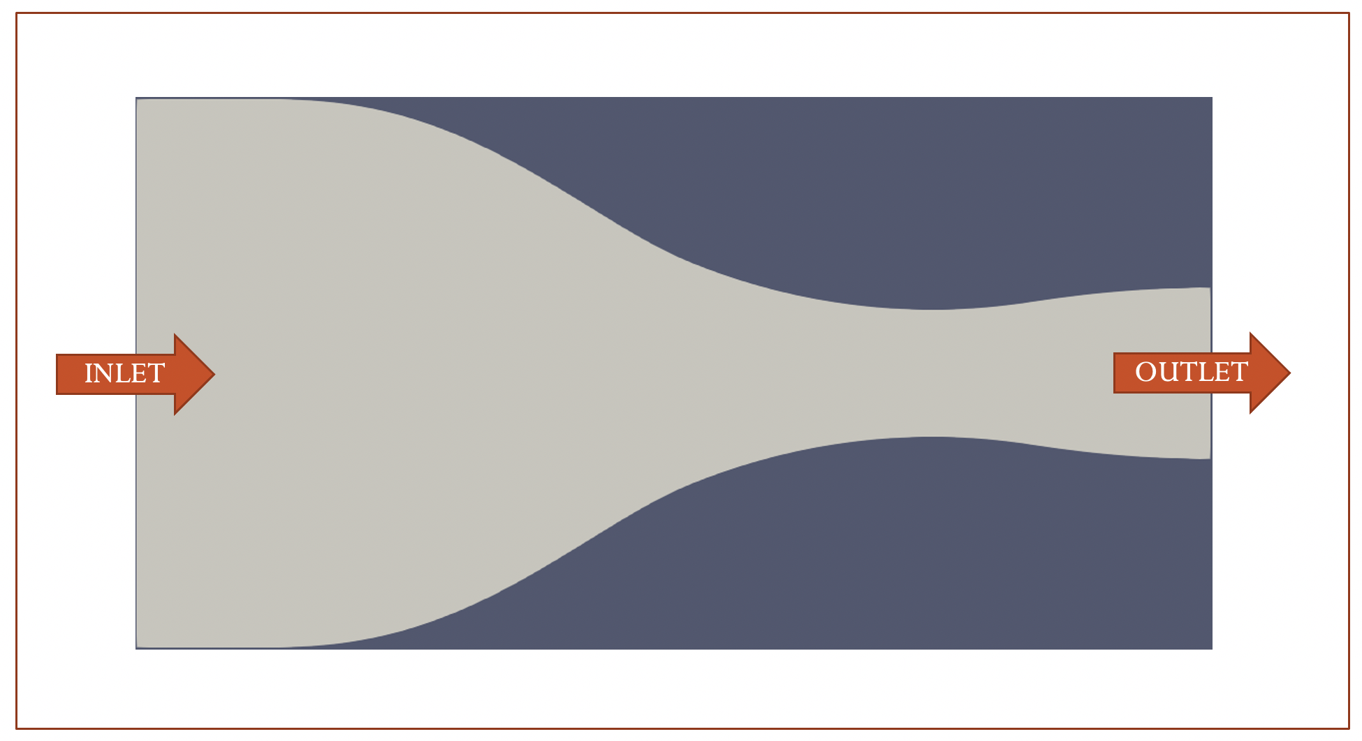
Figure 1: CD Nozzle

4.1 Test Case Description

Octamethyltrisiloxane (MDM), a pressure-sensitive fluid, is used as a working fluid for analyzing non-ideal supersonic compressible flow inside a converging-diverging (CD) nozzle. Table 1 presents details about the properties of fluid and flow conditions. This configuration results in a total exhaust pressure ratio of 3.125, which results in a supersonic outflow at Mach number 1.5 Guardone (2021). The static pressure applied to the test case’s outlet is 200,000 Pa. The computational domain and mesh are depicted in Figure 2. The mesh is composed of 3,540 quadrilateral elements and 3,660 nodes Guardone (2021). At the inlet and outlet boundaries, Riemann boundary conditions based on characteristics are used. Symmetry boundary conditions define symmetry boundaries. By mirroring the flow around the x-axis, the mesh size is reduced, along with the computational cost. On the boundary of a wall, Navier-Stokes adiabatic wall conditions are applied.

Table 1: Flow conditions for C-D Nozzle CFD simulation

Parameters	Values
Working fluid	Octamethyltrisiloxane
Inlet Pressure	904388 Pa
Inlet Temperature	542.13 K
Turbulence model	SST
Gamma Value	1.01767
Gas Constant	35.17
Critical Temperature	565.3609
Critical Pressure	1437500
$\mu$	1.21409E-05
$K_{T}$	0.030542828

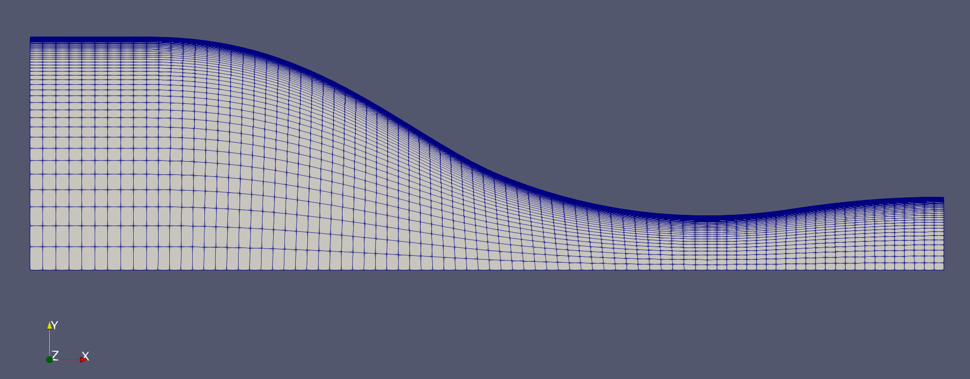
Figure 2: Computational domain and mesh

4.2 Deterministic Results

For deterministic simulations, the SU2 solver is run at the fixed boundary conditions, flow conditions, and fluid properties as described earlier. The total number of iteration was given 1000 so that all solutions and residuals are converged nicely. We post-process the data with Paraview (a multi-platform, open-source data analysis and visualization application). In Figure 4, solution fields for pressure, temperature, Mach number, and flow density are exhibited for the whole computational domain. Further, these quantities are also shown at the centerline of the nozzle for better understanding and analysis. At the inlet of the nozzle, pressure, temperature, and density of the fluid are at their maximum and then at their minimum near the outlet. In an inlet, the Mach number can be viewed as a minimum, and at the exit, the Mach number reaches a maximum value.

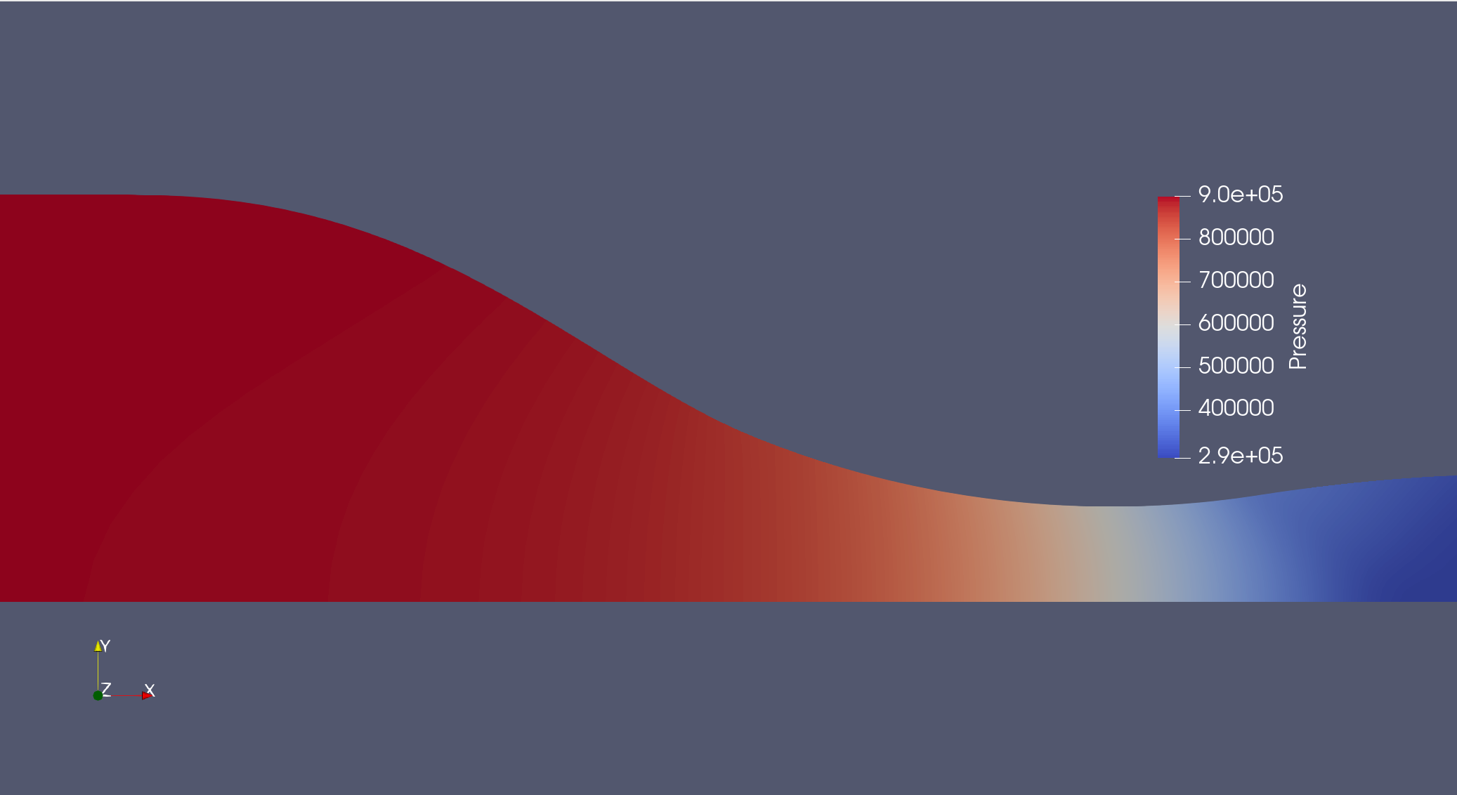
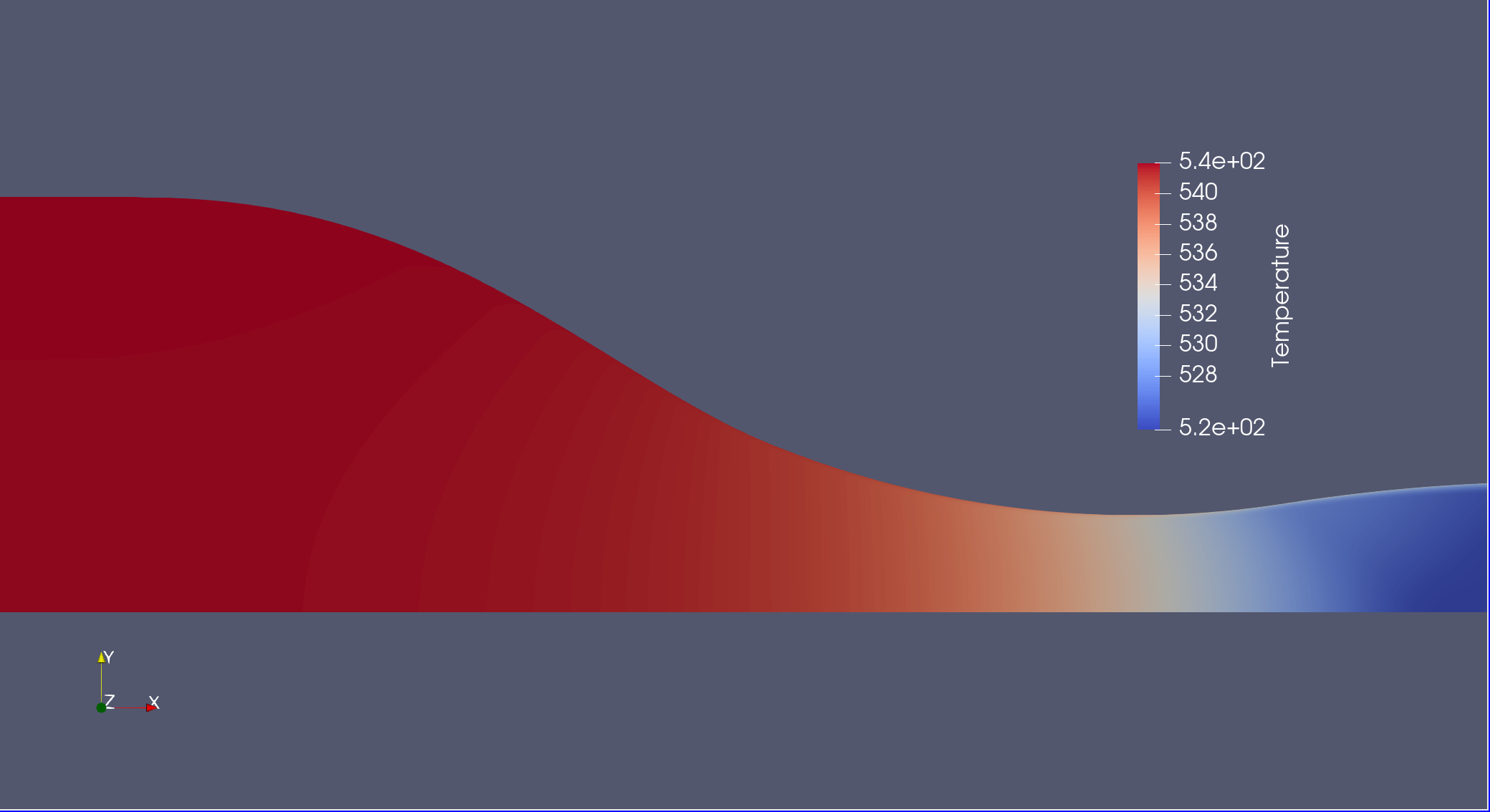
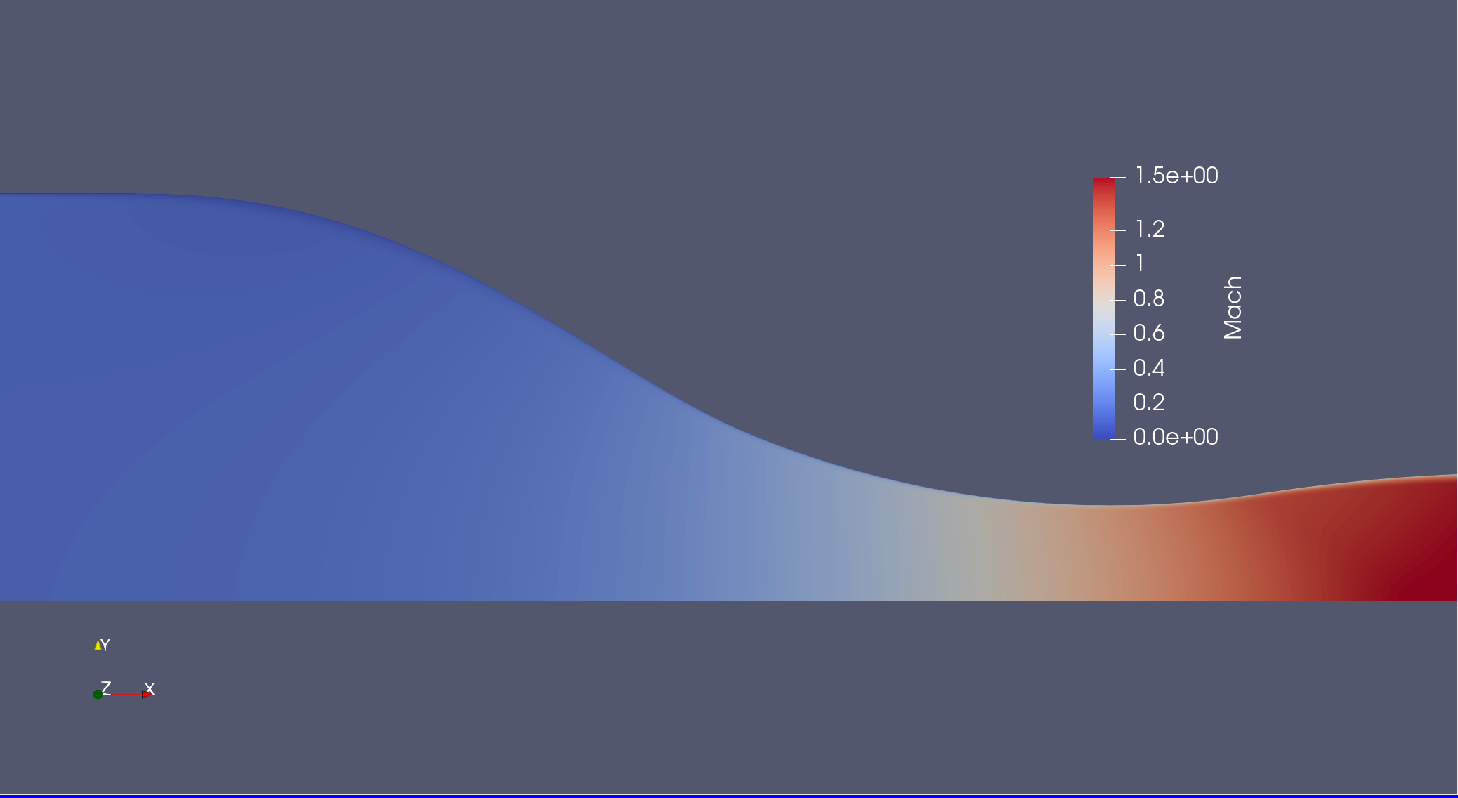
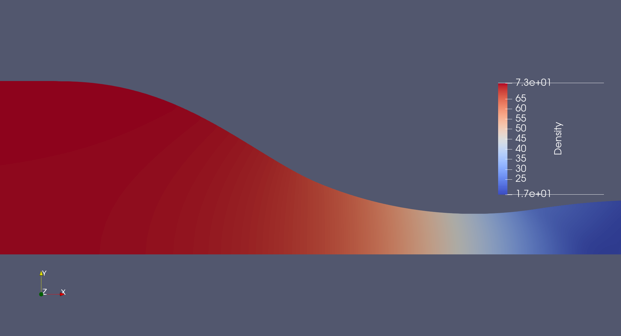
Figure 3: Numerical results (provided serially in vertical format): pressure, temperature, Mach, and density fields

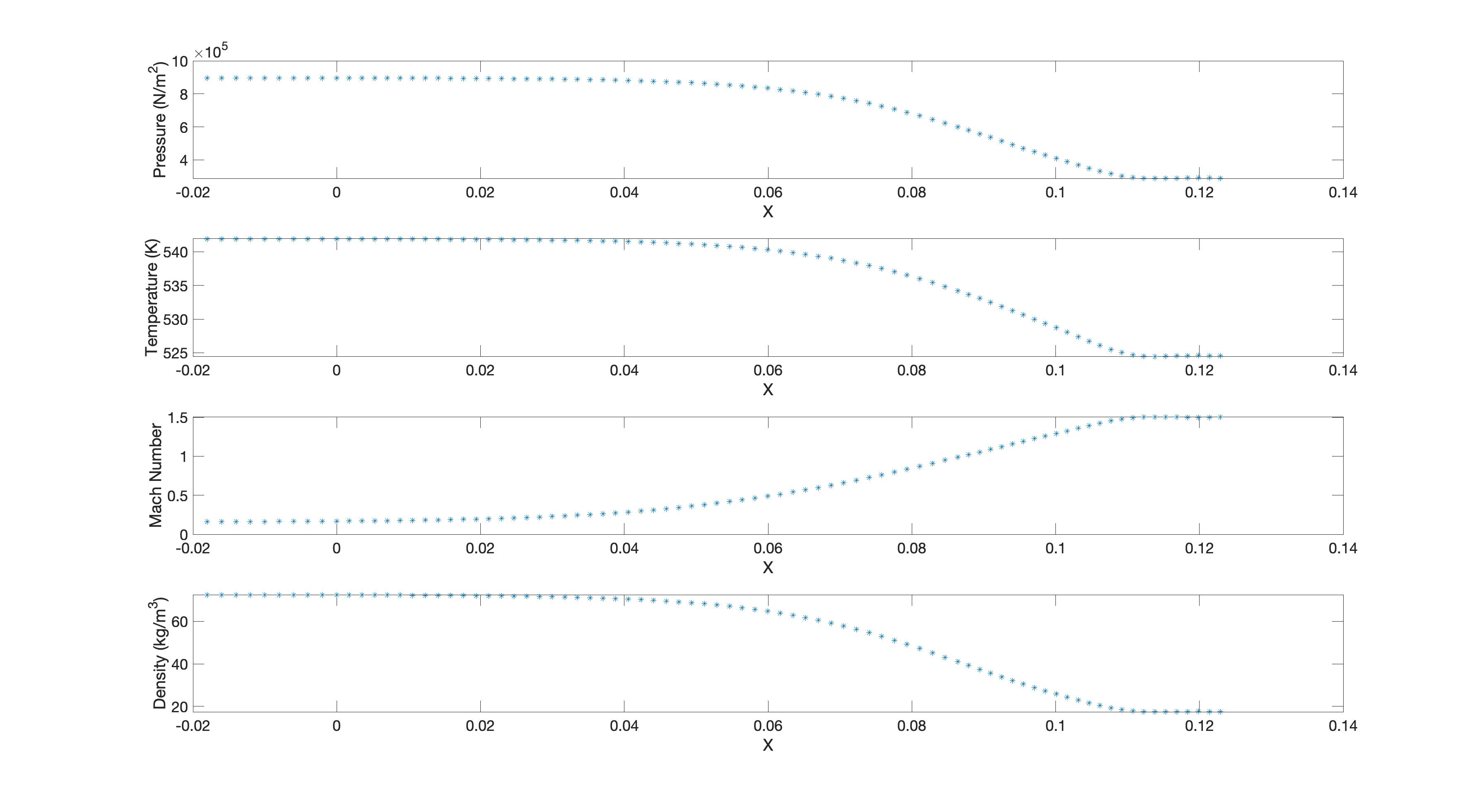
Figure 4: Computational results: pressure, temperature, Mach number and fluid density at the centerline of the nozzle )

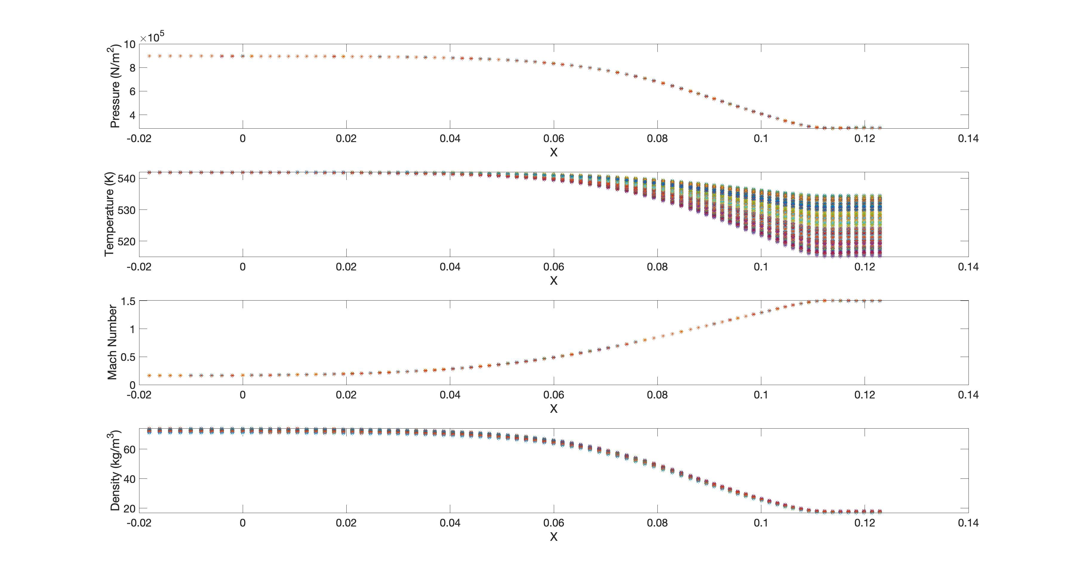
Figure 5: Solution samples for Pressure, Temperature, Mach number and fluid density at the centerline of the nozzle )

Figure 6: Mean and standard deviation for Pressure, Temperature, Mach number and fluid density at the centerline of the nozzle )

4.3 Description of Uncertainties

For the uncertainty analysis, seven input parameters; two from boundary values (inlet temperature and inlet pressure), three from gas properties (specific heat ratio $\gamma$, gas constant $R$ and acentric factor $\omega$), and two from the viscosity model (molecular viscosity $\mu$ and molecular thermal conductivity $K_{T}$) are considered as uncertain. All parameters are considered uniformly distributed. The inlet pressure and acentric factor are assumed to have $5\%$ variability from the mean value. Gas constant, molecular viscosity, and molecular thermal conductivity are assumed to vary $2\%$ from their mean values. Minor uncertainties of $1\%$ from their mean values are given to the inlet temperature and Gamma values. All the mean values for these parameters, their uncertainties, and their ranges of variability are described in Table 2.

Table 2: Input uncertainties for CFD simulations

Parameters	Values	Uncertainties ($\%$)	Minimum	Maximum
Inlet Pressure (Pa)	904388	5	859168	949607
Inlet Temperature (K)	542.13	1	536.71	547.55
Gamma Value	1.01767	1	1.00749	1.02785
Gas Constant	35.17	2	34.47	35.87
$\mu$	1.21409E-05	2	1.18981	1.23837
$K_{T}$	0.030542828	2	0.029931971	0.031153684
Acentric factor ($\omega$)	0.524	5	0.498	0.550

4.4 Uncertainty Analysis

As described in the previous section, the PC-Kriging method is used here to estimate the combined impact of all input uncertainties on the system responses of the CD nozzle. Usually, in the regression-based polynomial chaos method, a total of 240 CFD samples (for PC order 3 and 7 input uncertainties) will be required to estimate the statistical quantities (mean and standard deviance) of the output accurately (see Kumar et al. (2016)). Here to construct the PC-Kriging-based surrogate model, only 100 CFD simulations are used. For input parameters, 100 designs of experiments are constructed using the Sobol sequence-based sampling technique. In Figure 5, the CFD solutions for pressure, temperature, Mach number, and fluid density along the nozzle centerline are shown for all 100 samples. It can be seen that pressure and Mach number are not varying much with the input uncertainties. However, minor variations can be seen in density with the input variations. The most significant variations can be seen for the temperature field. In Figure 6, the mean and standard deviation are shown for all these quantities. These values are calculated from the PC-Kriging based surrogate model. The mean values behavior is similar to the deterministic solutions. For pressure, temperature, and Mach number, the standard deviation values are higher at the outlet. That means the highest fluctuations are at the nozzle outlet. However, the standard deviation for fluid density is seen lower at the nozzle outlet.

It is also important to address that this developed uncertainty method can be applied to other domains such as nuclear engineering in terms of safety assessment of advanced reactor system Kumar et al. (2021a). In addition, the authors also utilized this methodology to understand the evaluate the uncertainties in composite materials Kumar et al. (2021b).

5 Conclusions

In this work, first, we describe the two most popular meta-modeling methods (Polynomial Chaos and Kriging methods) suitable for uncertainty quantification in engineering applications. Further, to increase the efficiency, the polynomial chaos and Kriging methods are combined and used for an engineering test problem under multiple uncertainties. A 2D supersonic converging-diverging nozzle is considered for the analysis where the multi-physics CFD solver SU2 is used for deterministic solutions. The UQ methods (polynomial chaos, Kriging, and PC-Kriging) are developed in Matlab and are further combined with SU2 for uncertainty quantification. The standard deviation can be considered as a safety bound or a confidence interval around the mean values. Hence, for assurance in making crucial decisions, the results are discussed in terms of the mean and standard deviation of the output quantities, i.e., pressure, temperature, Mach number, and fluid density.

Future work will focus on its application in multiscale modeling of composite accident-tolerant nuclear fuels with Sic/Sic claddings for small modular reactor (SMR) applications.

References

- Oberkampf and Trucano [2002] William L Oberkampf and Timothy G Trucano. Verification and validation in computational fluid dynamics. Progress in aerospace sciences, 38(3):209–272, 2002.
- Roy and Oberkampf [2011] Christopher J Roy and William L Oberkampf. A comprehensive framework for verification, validation, and uncertainty quantification in scientific computing. Computer methods in applied mechanics and engineering, 200(25-28):2131–2144, 2011.
- Beyer and Sendhoff [2007] Hans-Georg Beyer and Bernhard Sendhoff. Robust optimization–a comprehensive survey. Computer methods in applied mechanics and engineering, 196(33-34):3190–3218, 2007.
- Schuëller and Jensen [2008] G.I. Schuëller and H. A. Jensen. Computational methods in optimization considering uncertainties - an overview. Computational Methods in Applied Mechanical Engineering, 198:2–13, 2008.
- Wiener [1938] Norbert Wiener. The homogeneous chaos. American Journal of Mathematics, 60(4):897–936, 1938.
- Xiu and Karniadakis [2002a] Dongbin Xiu and George Em Karniadakis. The wiener–askey polynomial chaos for stochastic differential equations. SIAM Journal on Scientific Computing, 24(2):619–644, 2002a.
- Smith [2013] Ralph C Smith. Uncertainty quantification: theory, implementation, and applications, volume 12. Siam, 2013.
- Kumar et al. [2021a] Dinesh Kumar, Syed Alam, Tuhfatur Ridwan, and Cameron S Goodwin. Quantitative risk assessment of a high power density small modular reactor (smr) core using uncertainty and sensitivity analyses. Energy, 227:120400, 2021a.
- Kumar et al. [2020a] Dinesh Kumar, SB Alam, Dean Vučinić, and C Lacor. Uncertainty quantification and robust optimization in engineering. In Advances in Visualization and Optimization Techniques for Multidisciplinary Research, pages 63–93. Springer, 2020a.
- Kabir et al. [2021a] HM Dipu Kabir, Abbas Khosravi, Subrota K Mondal, Mustaneer Rahman, Saeid Nahavandi, and Rajkumar Buyya. Uncertainty-aware decisions in cloud computing: Foundations and future directions. ACM Computing Surveys (CSUR), 54(4):1–30, 2021a.
- Kabir et al. [2021b] HM Dipu Kabir, Abbas Khosravi, Abdollah Kavousi-Fard, Saeid Nahavandi, and Dipti Srinivasan. Optimal uncertainty-guided neural network training. Applied Soft Computing, 99:106878, 2021b.
- Kabir et al. [2020] HM Dipu Kabir, Abbas Khosravi, Darius Nahavandi, and Saeid Nahavandi. Uncertainty quantification neural network from similarity and sensitivity. In 2020 International Joint Conference on Neural Networks (IJCNN), pages 1–8. IEEE, 2020.
- Kumar et al. [2021b] Dinesh Kumar, Mariapia Marchi, Syed Bahauddin Alam, Carlos Kavka, Yao Koutsawa, Gaston Rauchs, and Salim Belouettar. Multi-criteria decision making under uncertainties in composite materials selection and design. Composite Structures, page 114680, 2021b.
- Kumar et al. [2020b] D. Kumar, S.B. Alam, H. Sjöstrand, J.M. Palau, and C. De Saint Jean. Nuclear data adjustment using bayesian inference, diagnostics for model fit and influence of model parameters. In EPJ Web of Conferences, volume 239, page 13003. EDP Sciences, 2020b.
- Kumar et al. [2019] D. Kumar, S.B. Alam, H. Sjöstrand, J.M. Palau, and C. De Saint Jean. Influence of nuclear data parameters on integral experiment assimilation using cook’s distance. In EPJ Web of Conferences, volume 211, page 07001. EDP Sciences, 2019.
- Hirsch et al. [2018] Charles Hirsch, Dirk Wunsch, J Szumbarksi, L Laniewski-Wollk, and Jordi Pons-Prats. Uncertainty management for robust industrial design in aeronautics. Notes on Numerical Fluid Mechanics and Multidisciplinary Design, 140, 2018.
- Hammersley [2013] John Hammersley. Monte carlo methods. Springer Science & Business Media, 2013.
- Rubinstein and Kroese [2016] Reuven Y Rubinstein and Dirk P Kroese. Simulation and the Monte Carlo method, volume 10. John Wiley & Sons, 2016.
- Xiu and Karniadakis [2002b] Dongbin Xiu and George Em Karniadakis. The wiener–askey polynomial chaos for stochastic differential equations. SIAM journal on scientific computing, 24(2):619–644, 2002b.
- Najm [2009] Habib N Najm. Uncertainty quantification and polynomial chaos techniques in computational fluid dynamics. Annual review of fluid mechanics, 41:35–52, 2009.
- Hosder et al. [2007] Serhat Hosder, Robert Walters, and Michael Balch. Efficient sampling for non-intrusive polynomial chaos applications with multiple uncertain input variables. In 48th AIAA/ASME/ASCE/AHS/ASC Structures, Structural Dynamics, and Materials Conference, page 1939, 2007.
- Ghanem et al. [2017] Roger Ghanem, David Higdon, and Houman Owhadi. Handbook of uncertainty quantification, volume 6. Springer, 2017.
- Quinonero-Candela and Rasmussen [2005] Joaquin Quinonero-Candela and Carl Edward Rasmussen. A unifying view of sparse approximate gaussian process regression. The Journal of Machine Learning Research, 6:1939–1959, 2005.
- Bastos and O’Hagan [2009] Leonardo S Bastos and Anthony O’Hagan. Diagnostics for gaussian process emulators. Technometrics, 51(4):425–438, 2009.
- Awad and Khanna [2015] Mariette Awad and Rahul Khanna. Support vector regression. In Efficient learning machines, pages 67–80. Springer, 2015.
- Smola and Schölkopf [2004] Alex J Smola and Bernhard Schölkopf. A tutorial on support vector regression. Statistics and computing, 14(3):199–222, 2004.
- Schobi et al. [2015] Roland Schobi, Bruno Sudret, and Joe Wiart. Polynomial-chaos-based kriging. International Journal for Uncertainty Quantification, 5(2), 2015.
- Wang et al. [2019] Fenggang Wang, Fenfen Xiong, Shishi Chen, and Jianmei Song. Multi-fidelity uncertainty propagation using polynomial chaos and gaussian process modeling. Structural and Multidisciplinary Optimization, 60(4):1583–1604, 2019.
- Saltelli [2002] Andrea Saltelli. Sensitivity analysis for importance assessment. Risk analysis, 22(3):579–590, 2002.
- Sudret [2008] Bruno Sudret. Global sensitivity analysis using polynomial chaos expansions. Reliability engineering & system safety, 93(7):964–979, 2008.
- Kumar et al. [2020c] Dinesh Kumar, Yao Koutsawa, Gaston Rauchs, Mariapia Marchi, Carlos Kavka, and Salim Belouettar. Efficient uncertainty quantification and management in the early stage design of composite applications. Composite Structures, page 112538, 2020c.
- Blatman and Sudret [2011] Géraud Blatman and Bruno Sudret. Adaptive sparse polynomial chaos expansion based on least angle regression. Journal of computational Physics, 230(6):2345–2367, 2011.
- Liu et al. [2020] HB Liu, C Jiang, and Z Xiao. Efficient uncertainty propagation for parameterized p-box using sparse-decomposition-based polynomial chaos expansion. Mechanical Systems and Signal Processing, 138:106589, 2020.
- Kumar et al. [2016] Dinesh Kumar, Mehrdad Raisee, and Chris Lacor. An efficient non-intrusive reduced basis model for high dimensional stochastic problems in cfd. Computers & Fluids, 138:67–82, 2016.
- Aremu et al. [2020] Oluseun Omotola Aremu, David Hyland-Wood, and Peter Ross McAree. A machine learning approach to circumventing the curse of dimensionality in discontinuous time series machine data. Reliability Engineering & System Safety, 195:106706, 2020.
- Liu and Bellet [2019] Kuan Liu and Aurélien Bellet. Escaping the curse of dimensionality in similarity learning: Efficient frank-wolfe algorithm and generalization bounds. Neurocomputing, 333:185–199, 2019.
- Bourinet [2018] Jean-Marc Bourinet. Reliability analysis and optimal design under uncertainty-Focus on adaptive surrogate-based approaches. PhD thesis, Université Clermont Auvergne, 2018.
- Du [2019] Xiaosong Du. Efficient uncertainty propagation for model-assisted probability of detection and sensitivity analysis via metamodeling and multifidelity methods. PhD thesis, Iowa State University, 2019.
- Zhang and Apley [2016] Ning Zhang and Daniel W Apley. Brownian integrated covariance functions for gaussian process modeling: Sigmoidal versus localized basis functions. Journal of the American Statistical Association, 111(515):1182–1195, 2016.
- Tarantola et al. [1982] Albert Tarantola, Bernard Valette, et al. Inverse problems= quest for information. Journal of geophysics, 50(1):159–170, 1982.
- O’Hagan [1978] Anthony O’Hagan. Curve fitting and optimal design for prediction. Journal of the Royal Statistical Society: Series B (Methodological), 40(1):1–24, 1978.
- Hinton et al. [1995] Geoffrey E Hinton, Peter Dayan, Brendan J Frey, and Radford M Neal. The" wake-sleep" algorithm for unsupervised neural networks. Science, 268(5214):1158–1161, 1995.
- Williams and Rasmussen [1996] Christopher KI Williams and Carl Edward Rasmussen. Gaussian processes for regression. 1996.
- Gibbs and MacKay [1997] Mark Gibbs and David JC MacKay. Efficient implementation of gaussian processes. 1997.
- Girard [2004] Agathe Girard. Approximate methods for propagation of uncertainty with Gaussian process models. University of Glasgow (United Kingdom), 2004.
- Amini et al. [2021] A Amini, A Abdollahi, MA Hariri-Ardebili, and U Lall. Copula-based reliability and sensitivity analysis of aging dams: Adaptive kriging and polynomial chaos kriging methods. Applied Soft Computing, page 107524, 2021.
- Guardone [2021] Alberto Guardone. Non-ideal compressible flow in a supersonic nozzle. https://su2code.github.io/tutorials/NICFD_nozzle/, 2021.