On learning history based policies for controlling Markov decision processes

Abstract

Reinforcement learning (RL) folklore suggests that history-based function approximation methods, such as recurrent neural nets or history-based state abstraction, perform better than their memory-less counterparts, due to the fact that function approximation in Markov decision processes (MDP) can be viewed as inducing a Partially observable MDP. However, there has been little formal analysis of such history-based algorithms, as most existing frameworks focus exclusively on memory-less features. In this paper, we introduce a theoretical framework for studying the behaviour of RL algorithms that learn to control an MDP using history-based feature abstraction mappings. Furthermore, we use this framework to design a practical RL algorithm and we numerically evaluate its effectiveness on a set of continuous control tasks.

1 Introduction

State abstraction and function approximation are vital components used by reinforcement learning (RL) algorithms to efficiently solve complex control problems when exact computations are intractable due to large state and action spaces. Over the past few decades, state abstraction in RL has evolved from the use of pre-determined and problem-specific features [CritesB95, TsitsiklisR96, ndp, Sutton+Barto:1998, SinghLKW02, activesensing, ProperT06] to the use of adaptive basis functions learnt by solving an isolated regression problem [kbrl, autobasis-MenacheMS05, 6-keller, Petrik07], and more recently to the use of neural network-based Deep-RL algorithms that embed state abstraction in successive layers of a neural network [Barto2004SynthesisON, BellemareDDTCRS19].

Feature abstraction results in information loss, and the resulting state features might not satisfy the controlled Markov property, even if this property is satisfied by the corresponding state  [Sutton+Barto:2018]. One approach to counteract the loss of the Markov property is to generate the features using the history of state-action pairs, and empirical evidence suggests that using such history-based features are beneficial in practice [openai2019learning]. However, a theoretical characterisation of history-based Deep-RL algorithms for fully observed Markov Decision Processes (MDPs) is largely absent form the literature.

In this paper, we bridge this gap between theory and practise by providing a theoretical analysis of history-based RL agents acting in a MDP. Our approach adapts the notion of approximate information state (AIS) for POMDPs proposed in [ais-1, ais-2] to feature abstraction in MDPs, and we develop a theoretically grounded policy search algorithm for history-based feature abstractions and policies.

The rest of the paper is organised as follows: In Section 2, following a brief review of feature-based abstraction, we motivate the need for using history-based feature abstractions. In Section 3, we present a formal model for the co-design of the feature abstraction and control policy, derive a dynamic program using the AIS. We also derive bounds on the quality of approximate solutions to this dynamic program. In Section 4 we build on these approximation bounds to develop an RL algorithm for learning a history-based state representation and control policy. In Section 5, we present an empirical evaluation of our proposed algorithm on continuous control tasks. Finally, we discuss related work in Section 6 and conclude with future research directions in Section 7.

2 Background and Motivation

Consider an MDP $\mathcal{M}=\langle\mathcal{S},\mathcal{A},P,r,\gamma\rangle$ where $\mathcal{S}$ denotes the state space, $\mathcal{A}$ denotes the action space, $P$ denotes the controlled transition matrix, $r\colon\mathcal{S}\times\mathcal{A}\to$ denotes the per-step reward, and $\gamma\in(0,1)$ denotes the discount factor.

The performance of a randomised (and possibly history-dependent) policy $\pi$ starting from a start state $s_{0}$ is measured by the value function, defined as:

$$V^{\pi}(s_{0})=\underset{\begin{subarray}{c}\end{subarray}}{\mathbb{E}}^{\pi}\bigg{[}\sum_{t=1}^{\infty}\gamma^{t-1}r(S_{t},A_{t})\bigg{|}S_{0}=s_{0}\bigg{]}.$$ (1)

A policy maximising $V^{\pi}(s_{0})$ over all (randomised and possibly history dependent) policies is called the optimal policy with respect to initial state $s_{0}$ and is denoted by $\pi^{\star}$.

In many applications, $\mathcal{S}$ and $\mathcal{A}$ are combinatorially large or uncountable, which makes it intractable to compute the optimal policy. Most practical RL algorithms overcome this hurdle by using function approximation where the state is mapped to a feature space $\mathcal{Z}$ using a state abstraction function $\phi:\mathcal{S}\to\mathcal{Z}$. In Deep-RL algorithms, the last layer of the network is often viewed as a feature vector. These feature vectors are then used as an approximate state for approximating the value function $\hat{V}:\mathcal{Z}\to$ and/or computing an approximately optimal policy $\mu:\mathcal{Z}\to\Delta(\mathcal{A})$ [Sutton+Barto:1998] (where $\Delta(\mathcal{A})$ denotes the set of probability distribution over actions). Therefore, the mapping from state to distribution of actions is given by the “flattened” policy $\tilde{\mu}=\mu\circ\phi$  i.e., $\tilde{\mu}=\mu(\phi(\cdot))$.

A well known fact about function approximation is that the features that are used as an approximate state may not satisfy the controlled Markov property i.e., in general,

$$\mathds{P}(Z_{t+1}\mid Z_{1:t},A_{1:t})\neq\mathds{P}(Z_{t+1}\mid Z_{t},A_{t}).$$

(a) $P(0)$

(b) $P(1)$

(c) $P(2)$

(d) $P_{\pi{}}$

Figure 1: The transition probability for an example MDP

To see the implications of this fact, consider the toy MDP depicted in Fig. 1a, 1b and 1c, with $\mathcal{S}=\{0,1,2,3\}$, $\mathcal{A}=\{0,1,2\}$, $\{P_{s,s^{\prime}}(a)\}_{a\in\mathcal{A}}$, and $r(0)=r(1)=-1$, $r(2)=1$, $r(3)=-K$, where $K$ is a large positive number. Given the reward structure the objective of the policy is to try to avoid state $3$ and keep the agent at state $2$ as much as possible. It is easy to see that the optimal policy is

$$\pi^{\star}(0)=0,\quad\pi^{\star}(1)=0,\quad\pi^{\star}(2)=1,\text{ and}\quad\pi^{\star}(3)=2.$$

Note that if the initial state is not state $3$ then an agent will never visit that state under the optimal policy. Furthermore, any policy which cannot prevent the agent from visiting state $3$ will have a large negative value and, therefore, cannot be optimal. Now suppose the feature space $\mathcal{Z}=\{0,1\}$. It is easy to see that for any Markovian feature-abstraction $\phi{}\colon\mathcal{S}\to\mathcal{Z}$, no policy $\hat{\pi}\colon\mathcal{Z}\to\mathcal{A}$ can prevent the agent from visiting state $3$. Thus, the best policy when using Markovian feature abstraction will perform significantly worse than the optimal policy (which has direct access to the state).

However, it is possible to construct a history-based feature-abstraction $\phi$ and a history-based control policy $\hat{\pi}$ that works with $\phi$ and is of the same quality as $\pi^{\star}$. For this, consider the following codebooks (where the entries denoted by a dot do not matter):

The Markov chain induced by the optimal policy is shown in Fig. 1d. Now define

$$F(1) =\begin{bmatrix}0&1&\cdot&\cdot\\ \cdot&0&1&\cdot\\ \cdot&\cdot&0&1\\ 1&\cdot&\cdot&0\end{bmatrix}, F(2) =\begin{bmatrix}1&\cdot&\cdot&0\\ 0&1&\cdot&\cdot\\ \cdot&0&1&\cdot\\ \cdot&\cdot&0&1\end{bmatrix}, F(3) =\begin{bmatrix}\cdot&0&\cdot&1\\ 0&\cdot&1&\cdot\\ \cdot&0&\cdot&1\\ 0&\cdot&1&\cdot\end{bmatrix},$$

$$D(0) =\begin{bmatrix}0&1\\ 1&2\\ 2&3\\ 3&0\end{bmatrix}, D(1) =\begin{bmatrix}3&0\\ 0&1\\ 1&2\\ 2&3\end{bmatrix}, D(2) =\begin{bmatrix}1&3\\ 0&2\\ 1&3\\ 0&2\end{bmatrix}.$$

and consider the feature-abstraction policy $Z_{t}=F_{S_{t-1},S_{t}}(A_{t-1})$ and a control policy $\mu$ which is a finite state machine with memory, where the memory $M_{t}$ that is updated as $M_{t}=D_{M_{t-1},Z_{t}}(A_{t-1})$ and the action $A_{t}$ is chosen as $A_{t}=\pi(M_{t}),$ where $\pi\colon\mathcal{S}\to\Delta(\mathcal{A})$ is any pre-specified reference policy. It can be verified that if the system starts from a known initial state then $\mu\circ\phi=\pi$. Thus, if we choose the reference policy $\pi=\pi^{\star}$, then the agent will never visit state $3$ under $\mu\circ\phi$, in contrast to Markovian feature-abstraction policies where (as we argued before) state $3$ is always visited.

In the above example, we used the properties of the system dynamics and the reward function to design a history-based feature abstraction which outperforms memoryless feature abstractions. We are interested in developing such history-based feature abstractions using a learning framework when the system model is not known. We present such a construction in the next section.

3 Approximation bounds for history-based feature abstraction

The approximation results of our framework depend on the properties of metrics on probability spaces. We start with a brief overview of a general class of metrics known as Integral Probability Measures (IPMs) [ipm]; many of the commonly used metrics on probability spaces such as total variation (TV) distance, Wasserstein distance, and maximum-mean discrepency (MMD) are instances of IPMs. We then derive a general approximation bound that holds for general IPMs, and then specialize the bound to specific instances (TV, Wassserstein, and MMD).

3.1 Integral probability metrics (IPM)

Definition 3.1 ( [ipm]).

Let $(\mathcal{E},\mathcal{G})$ be a measurable space and $\mathfrak{F}$ denote a class of uniformly bounded measurable functions on $(\mathcal{E},\mathcal{G})$. The integral probability metric between two probability distributions $\nu_{1},\nu_{2}\in\mathcal{P}(\mathcal{E})$ with respect to the function class $\mathfrak{F}$ is defined as:

$$d_{\mathfrak{F}}(\nu_{1},\nu_{2}) =\sup_{f\in\mathfrak{F}}\bigg{|}\int_{\mathcal{E}}fd\nu_{1}-\int_{\mathcal{E}}fd\nu_{2}\bigg{|}.$$ (2)

For any function $f$ (not necessarily in $\mathfrak{F}$), the Minkowski functional $\rho_{\mathfrak{F}}$ associated with the metric $d_{\mathfrak{F}}$ is defined as:

$$\rho_{\mathfrak{F}}(f) \triangleq\inf\{\rho\in_{\geq 0}:\rho^{-1}f\in\mathfrak{F}\}.$$ (3)

Eq. (3), implies that that for any function $f$:

$$\bigg{|}\int_{\mathcal{E}}fd\nu_{1}-\int_{\mathcal{E}}fd\nu_{2}\bigg{|}\leq\rho_{\mathfrak{F}}(f)d_{\mathfrak{F}}(\nu_{1},\nu_{2}).$$ (4)

In this paper, we use the following IPMs:

• Total Variation Distance: If $\mathfrak{F}$ is chosen as $\mathfrak{F}^{\text{TV}}\triangleq\{\frac{1}{2}\operatorname{span}(f)$ = $\frac{1}{2}(\max(f)-\min(f))\}$, then $d_{\mathfrak{F}}$ is the total variation distance, and its Minkowski functional is $\rho_{\mathfrak{F}^{\text{TV}}}(f)=\frac{1}{2}\operatorname{span}(f)$.

• Wasserstein/Kantorovich-Rubinstein Distance: If $\mathcal{E}$ is a metric space and $\mathfrak{F}$ is chosen as $\mathfrak{F}^{W}\triangleq\{f:L_{f}\leq 1\}$ (where $L_{f}$ denotes the Lipschitz constant of $f$ with respect to the metric on $\mathcal{E}$), then $d_{\mathfrak{F}}$ is the Wasserstein or the Kantorovich distance. The Minkowski function for the Wasserstein distance is $\rho_{\mathfrak{F}^{W}}(f)=L_{f}$.

• Maximum Mean Discrepancy (MMD) Distance: Let $\mathcal{U}$ be a reproducing kernel Hilbert space (RKHS) of real-valued functions on $\mathcal{E}$ and $\mathfrak{F}$ is choosen as $\mathfrak{F}^{MMD}\triangleq\{f\in\mathcal{U}:\|f\|_{\mathcal{U}}\leq 1\}$, (where $\|\cdot\|_{\mathcal{U}}$ denotes the RKHS norm), then $d_{\mathfrak{F}}$ is the Maximum Mean Discrepancy (MMD) distance and its Minkowski functional is $\rho_{\mathfrak{F}^{\text{MMD}}}(f)=\|f\|_{\mathcal{U}}$.

3.2 Approximate information state

Given an MDP $\mathcal{M}$ and a feature space $\mathcal{Z}$, let $\mathcal{H}_{t}=\mathcal{S}\times\mathcal{A}$ denote the space of all histories $(S_{1:t},A_{1:t-1})$ up to time $t$, where $S_{1:t}$ is a shorthand notation for the history of states $(S_{1},\ldots,S_{t})$, and similar interpretation holds for $A_{1:t}$. We are interested in learning history-based feature abstraction functions $\{\sigma_{t}\colon\mathcal{H}_{t}\to\mathcal{Z}\}_{t\geq 1}$ and a time homogenous policy $\mu\colon\mathcal{Z}\to\Delta(\mathcal{A})$ such that the flattened policy $\pi{}=\{\pi{}_{t}\}_{t\geq 1}$, where $\pi{}_{t}=\mu\circ\sigma_{t}$, is approximately optimal.

Since the feature abstraction approximates the state, its quality depends on how well it can be used to approximate the per step reward and predict the next state. We formalise this intuition in definition below.

Definition 3.2.

A family of history-based feature abstraction functions $\{\sigma_{t}:\mathcal{H}_{t}\to\mathcal{Z}\}_{t\geq 1}$ are said to be recursively updatable if there exists an update function $\hat{f}:\mathcal{Z}\times\mathcal{S}\times\mathcal{A}\to\mathcal{Z}$ such that the process $\{Z_{t}\}_{t\geq 1}$, where $Z_{t}=\sigma_{t}(S_{1:t},A_{1:t-1})$, satisfies:

$$Z_{t+1}=\hat{f}(Z_{t},S_{t+1},A_{t}).\quad t\geq 1$$ (5)

Definition 3.3.

Given a family of history based recursively updatable feature abstraction functions $\{\sigma_{t}:\mathcal{H}_{t}\to\mathcal{Z}\}_{t\geq 1}$, the features $Z_{t}=\sigma_{t}(S_{1:t},A_{1:t-1})$ are said to be $(\epsilon,\delta)$-approximate information state (AIS) with respect to a function space $\mathfrak{F}$ if there exist: (i) a reward approximation function $\hat{r}:\mathcal{Z}\times\mathcal{A}\to$, and (ii) an approximate transition kernel $\hat{P}:\mathcal{Z}\times\mathcal{A}\to\Delta(\mathcal{S})$ such that $Z$ satisfies the following properties:

• Sufficient for approximate performance evaluation: for all $t$,

  $$|r(S_{t},A_{t})-\hat{r}(Z_{t},A_{t})|\leq\epsilon.$$ (6)

• Sufficient for predicting future states approximately: for all $t$

  $$d_{\mathfrak{F}}(P(\cdot|S_{t},A_{t}),\hat{P}(\cdot|Z_{t},A_{t}))\leq\delta.$$ (7)

We call the tuple $(\hat{r},\hat{P})$ as an $(\epsilon,\delta)$-AIS approximator. Note that similar definitions have appeared in other works e.g., latent state [deepmdp], and approximate information state for for POMDPs [ais-1, ais-2]. However, in [deepmdp] it is assumed that the feature abstractions are memory-less and the discussion is restricted to Wasserstein distance. The key difference from the POMDP model in [ais-1, ais-2] is that the in POMDPs the observation $Z_{t}$ is a pre-specified function of the state while in the proposed model $Z_{t}$ depends on our choice of feature abstraction.

As such, our key insight is that an AIS-approximator of a recursively updatable history-based feature abstraction can be used to define a dynamic program. In particular, given a history-based abstraction function $\{\sigma_{t}:\mathcal{H}_{t}\to\mathcal{Z}\}_{t\geq 1}$ which is recursively updatable using $\hat{f}$ and an $(\epsilon,\delta)$ AIS-approximator $(\hat{P},\hat{r})$, we can define the following dynamic programming decomposition:

For any $z_{t}\in\mathcal{Z},\ a_{t}\in\mathcal{A}$

$$\hat{Q}(z_{t},a_{t})=\hat{r}(z_{t},a_{t})+\gamma\sum_{s_{t+1}\in\mathcal{S}}\hat{P}(s_{t+1}|z_{t},a_{t})\hat{V}(\hat{f}(z_{t},s_{t+1},a_{t})); \hat{V}(z_{t})=\max_{a_{t}\in\mathcal{A}}\hat{Q}(z_{t},a_{t}),\quad\forall z_{t}\in\mathcal{Z}$$ (8a)

Definition 3.4.

Define $\mu\colon\mathcal{Z}\to\Delta(\mathcal{A})$ be any policy such that for any $z\in\mathcal{Z}$,

$$\operatorname{Supp}(\mu(z))\subseteq\arg\max_{a\in\mathcal{A}}\hat{Q}(z,a).$$ (9)

Since $\mu$ is a policy from the feature space to actions, we can use it to define a policy from the history of the state action pairs to actions as:

$$\pi{}_{t}(s_{1:t},a_{1:t-1})\triangleq\mu(\sigma_{t}(s_{1:t},a_{1:t-1}))$$ (10)

Therefore, the dynamic program defined in (8) indirectly defines a history-based policy $\pi{}$. The performance of any such history-based policy is given by the following dynamic program:

For any $z\in\mathcal{Z},\ a\in\mathcal{A}$

$$Q^{\pi{}}_{t}(h_{t},a_{t})=r(s_{t},a_{t})+\gamma\sum_{s_{t+1}\in\mathcal{S}}P(s_{t+1}|s_{t},a_{t})V_{t+1}^{\pi{}}(h_{t+1}); V_{t}^{\pi{}}(h_{t})=\max_{a\in\mathcal{A}}Q_{t}^{\pi{}}(h_{t},a_{t}),$$ (11a)

We want to quantify the loss in performance when using the history based policy $\pi$. Note that since $V_{t}^{\pi}$ is not time-homogeneous, we need to compute the worst-case difference between $V^{\star}$ and $V_{t}^{\pi}$, which is given by:

$$\Delta\triangleq\sup_{t\geq 0}\sup_{h_{t}=(s_{1:t},a_{1:t})\in\mathcal{H}_{t}}|V^{\star}(s_{t})-V^{\pi{}}_{t}(h_{t})|,$$ (12)

Our main approximation result is the following:

Theorem 3.5.

The worst case difference between $V^{\star}$ and $V^{\pi{}}_{t}$ is bounded by

$$\Delta\leq 2\frac{\varepsilon+\gamma\delta\kappa_{\mathfrak{F}}(\hat{V}^{\mu},\hat{f})}{1-\gamma},$$ (13)

where $\kappa_{\mathfrak{F}}(\hat{V}^{\mu},\hat{f})$ = $\sup_{z,a}\rho_{\mathfrak{F}}(\hat{V}^{\mu}(\hat{f}(\cdot,z,a)))$, $\rho_{\mathfrak{F}}(\cdot)$ is the Minkowski functional associated with the IPM $d_{\mathfrak{F}}$ as defined in (3).

Proof in Appendix A

Some salient features of the bound are as follows: First, the bound depends on the choice of metric on probability spaces. Different IPMs will result in a different value of $\delta$ and also a different value of $\kappa_{\mathfrak{F}}(\hat{V}^{\mu},\hat{f})$. Second, the bound depends on the properties of $\hat{V}^{\mu}$. For this reason we call it an instance dependent bound. Sometimes, it is desirable to have bounds which do not require solving the dynamic program in (8). We present such bounds as below, note that these “instance independent” bounds are the derived by upper bounding $\kappa_{\mathfrak{F}}(\hat{V}^{\mu},\hat{f})$. Therefore, these are looser than the upper bound in Theorem 3.5

Corollary 3.6.

If the function class $\mathfrak{F}$ is $\mathfrak{F}^{\text{TV}}$, then $\Delta$ as defined in (12) is upper bounded as:

$$\Delta\leq\frac{2\epsilon}{(1-\gamma)}+\frac{\gamma\delta\operatorname{span}(\hat{r})}{(1-\gamma)^{2}}.$$ (14)

Proof in Appendix B

Corollary 3.7.

Let $L_{\hat{r}}$ and $L_{\hat{P}}$ denote the Lipschitz constants of the approximate reward function $\hat{r}$ and approximate transition function $\hat{P}$ respectively, and $L_{\hat{f}}$ is the uniform bound on the Lipschitz constant of $\hat{f}$ with respect to the state $S_{t}$. If $\gamma L_{\hat{P}}L_{\hat{f}}\leq 1$ and the function class $\mathfrak{F}$ is $\mathfrak{F}^{\text{W}}$, then $\Delta$ as defined in (12) is upper bounded as:

$$\Delta\leq\frac{2\epsilon}{(1-\gamma)}+\frac{2\gamma\delta L_{\hat{r}}}{(1-\gamma)(1-\gamma L_{\hat{f}}L_{\hat{P}})}.$$ (15)

Proof in Appendix C

Corollary 3.8.

If the function class $\mathfrak{F}$ is $\mathfrak{F}^{\text{MMD}}$, then $\Delta$ as defined in (12) is upper bounded as:

$$\Delta\leq 2\frac{\epsilon+\gamma\delta\kappa_{\mathcal{U}}(\hat{V},\hat{f})}{(1-\gamma)},$$ (16)

where $\mathcal{U}$ is a RKHS space, $\|\cdot\|_{\mathcal{U}}$ its associated norm and $\kappa_{\mathcal{U}}(\hat{V},\hat{f})=\sup_{z,a}\|(\hat{V}(\hat{f}(\cdot,z,a)))\|_{\mathcal{U}}$.

Proof 3.9.

The proof follows from the properties of MMD described previously.

In the following section we will show how one can use these theoretical insights to design a policy search algorithm.

4 Reinforcement learning with history-based feature abstraction

In this section, we leverage the approximation bounds of Theorem 3.5 to develop a reinforcement learning algorithm. The main idea is to add an additional block, which we call the AIS-approximator, to any standard RL algorithm. In this section, we explain an AIS-based generalization for policy-based algorithms such as REINFORCE and actor-critic, but the same idea could be used for value-based algorithms such as Q-learning as well.

Figure 2: AIS approximator block

The AIS-approximator consists of two blocks: a recursively updatable history compressor and a reward and next-state predictor as shown in Fig. 2. In particular, we can consider any parameterised family of the history compression functions $\{\sigma_{t}(\cdot);\zeta)\colon\mathcal{H}_{t}\to\mathcal{Z}\}$ which are recursively updatable via the function $\hat{f}(\cdot)\colon\mathcal{Z}\times\mathcal{S}\times\mathcal{A}\to\mathcal{Z}$ as the history-compressor along with any parameterised family of functions $\hat{r}(\cdot;\zeta)\colon\mathcal{Z}\times\mathcal{A}\to$ as the reward approximator and any parameterised stochastic kernels ${\hat{P}}(\cdot;\zeta)\colon\mathcal{Z}\times\mathcal{A}\to\Delta(\mathcal{S})$ as the transition approximator. In the above notation $\zeta$ denotes the combined parameters of the family of functions. As a concrete example, we could use use memory-based neural networks such as LSTMs or GRUs as the history-compression functions. The memory update functions of such networks correspond to the update function $\hat{f}$. A multilayered perceptron (MLP) could be used as a reward approximator and a parameterized family of stochastic kernels such as the softmax function or a mixture of Gaussians could be used as the transition approximator. The parameters of all these networks together are denoted by $\zeta$.

We use a weighted combination of the reward prediction loss $|r(S_{t},A_{t})-\hat{r}(Z_{t},A_{t})|$ and the transition-prediction loss $d_{\mathfrak{F}}(P,\hat{P})$ as the loss function for the AIS-generator. In particular, the AIS-loss is given by

$$\mathcal{L}_{\text{AIS}}(\zeta) =\frac{1}{T}\sum_{t=0}^{T}\bigg{(}\lambda\underbrace{({\hat{r}}(Z_{t},A_{t};\zeta)-r(S_{t},A_{t}))^{2}}_{\mathcal{L}_{\hat{R}(\cdot;\zeta)}}+(1-\lambda)\cdot\underbrace{d_{\mathfrak{F}}({\hat{P}}(Z_{t},A_{t}\ ;\zeta),P)^{2}}_{\mathcal{L}_{\hat{P}}(\cdot;\zeta)}\bigg{)},$$ (17)

where $T$ is the length of the episode or the rollout length, $\lambda\in[0,1]$ is a hyper-parameter. The computation of $\mathcal{L}_{\hat{P}}(\cdot;\zeta)$, depends on the choice of IPM. In principle we can pick any IPM, but we would want to use an IPM using which the distance $d_{\mathfrak{F}}$ can be efficiently computed.

4.1 Choice of an IPM

To compute the IPM $d_{\mathfrak{F}}$ we need to know the probability density functions $\hat{P}$ and $P$. As we assume $\hat{P}$ to belongs to a parametric family, we know its density function in closed form. However, since we are in the learning setup, we can only access samples from $P$. For a function a $f\in\mathfrak{F}$, and probability density functions $P$ and $\hat{P}$ such that, $\nu_{1}=P$, and $\nu_{2}=\hat{P}$, we can estimate the IPM $d_{\mathfrak{F}}$ between a distribution and samples using the duality $|\int_{\mathcal{Z}}fd\nu_{1}-\int_{\mathcal{Z}}fd\nu_{2}|$. In this paper, we use two from of IPMs, the MMD distance and the Wasserstein/Kantorovich–Rubinstein distance.

4.1.1 MMD Distance:

Let $m_{\zeta}$ denote the mean of the distribution $\hat{P}(\cdot;\zeta)$. Then, the AIS-loss when MMD is used as an IPM is given by

$$\mathcal{L}_{\text{AIS}}(\zeta) =\frac{1}{T}\sum_{t=0}^{T}\bigg{(}\lambda({\hat{r}}(Z_{t},A_{t};\zeta)-r(S_{t},A_{t}))^{2}+(1-\lambda)(m^{S_{t}}_{\zeta}-2S_{t})^{\top}m^{S_{t}}_{\zeta}\bigg{)},$$ (18)

where $m^{S_{t}}_{\zeta}$ is obtained using the from the transition approximator,  i.e., the mapping ${\hat{P}}(\zeta):\mathcal{Z}\times\mathcal{A}\to$. For the detailed derivation of the above loss see Subsection D.1.1

4.1.2 Wasserstein/Kantorovich–Rubinstein distance:

In principle, the Wasserstein/Kantorovich distance can be computed by solving a linear program [Sriperumbudur], but doing at every episode can be computationally expensive. Therefore, we propose to approximate the Wasserstein distance using a KL-divergence [kl] based upper-bound. The simplified-KL divergence based AIS loss is given as:

$$\mathcal{L}_{\text{AIS}}(\zeta) =\frac{1}{T}\sum_{t=0}^{T}\bigg{(}\lambda({\hat{r}}(Z_{t},A_{t};\zeta)-r(S_{t},A_{t}))^{2}+(1-\lambda)\log(\hat{P}(S_{t};\zeta))\bigg{)},$$ (19)

where after dropping the terms which do not depend on $\zeta$, we get $d_{\mathfrak{F}^{\text{W}}}^{2}(P,\hat{P})\leq\log(\hat{P}(S_{t};\zeta))$ is the simplified-KL-divergence based upper bound. For the details of this derivation see Subsection D.1.2.

4.2 Policy gradient algorithm

Input : $\iota_{0}$: Initial state distribution,

$\zeta_{0}$: Ais parameters,

$\xi_{0}$: Actor parameters,

$a_{0}$: Initial action,

$\mathcal{D}=\emptyset$: Replay buffer,

$N_{\text{comp}}$: Computation budget,

$N_{\text{ep}}$: Episode length,

$N_{\text{grad}}$: Gradient steps

1 for iterations $i=0:N_{\text{comp}}$  do

2       Sample start state $s_{0}\sim\iota_{0}$;

3       for iterations $j=0:N_{\text{ep}}$  do

4             $z_{j}=\sigma_{\zeta}(s_{1:j},a_{1:j-1})$;

5             $a_{j}=\mu_{\xi}(z_{j})$;

6             $s_{j+1}=P(s_{j},a_{j})$;

7             $\mathcal{D}\xleftarrow{}\{z_{j},a_{j},s_{j},s_{j+1}\}$;

8             $a_{j-1}=a_{j}$;

9             $s_{j}=s_{j+1}$;

10            

11       end for

12      for every batch $b\in\mathcal{D}$ do

13             for gradient step $t=0:N_{\text{grad}}$ do

14                   $\zeta_{t+1,b}=\zeta_{t,b}+b\nabla_{\zeta}\mathcal{L}_{\text{AIS}}(\zeta_{t,b})$;

15                   $\xi_{t+1,b}=\xi_{t,b}+d\hat{\nabla}_{\xi}J(\xi_{t,b},\zeta_{t,b})$

16             end for

17            

18       end for

19      

20 end for

Algorithm 1 Policy Search with AIS

Following the design of the AIS block, we now provide a policy-gradient algorithm to learning both the AIS and policy. The schematic of our agent architecture is given in Fig. 2, and pseudo-code is given in Algorithm 1. Given a feature space $\mathcal{Z}$, we can simultaneously learn the AIS-generator and the policy using a multi-timescale stochastic gradient ascent algorithm [borkar2008stochastic]. Let $\mu(\cdot;\xi):\mathcal{Z}\to\Delta(\mathcal{A})$ be a parameterised stochastic policy with parameters $\xi$. Let $J(\xi,\zeta)$ denote the performance of the policy $\mu(\cdot;\ \xi)$. The policy gradient theorem [pgt, Williams2004SimpleSG, baxter-bartlett] states that: For a rollout horizon $T$, we can estimate $\nabla_{\xi}J$ as:

$$\hat{\nabla}_{\xi}J(\xi_{t},\zeta_{t}) =\sum_{t=1}^{T}\gamma^{t-1}r_{t}\bigg{(}\sum_{\tau=1}^{t}\nabla_{\xi}\log(\mu(A_{t}|Z_{t};\ \xi_{t}))\bigg{)}.$$

Following a rollout of length $T$, we can then update the parameters $\{(\zeta_{i},\xi_{i})\}_{i\geq 1}$ as follows:

$$\zeta_{i+1}=\zeta_{i}+b_{i}\nabla_{\zeta}\mathcal{L}_{\text{AIS}}(\zeta_{i}), \xi_{i+1}=\xi_{i}+d_{i}\hat{\nabla}_{\xi}J(\xi_{i},\zeta_{i}),$$ (20a)

where the step-size $\{b_{i}\}_{i\geq 0}$ and $\{d_{i}\}_{i\geq 0}$ satisfy the standard conditions $\sum_{i}b_{i}=\infty$, $\sum_{i}b_{i}^{2}<\infty$, $\sum_{i}d_{i}=\infty$ and $\sum_{i}d_{i}^{2}<\infty$ respectively. Moreover, one can ensure that the AIS generator converges faster by choosing an appropriate learning rates such that, $\lim_{i\to\infty}\frac{d_{i}}{b_{i}}=0$.

4.3 Actor Critic Algorithm

We can also use the aforementioned ideas to design an AIS based actor-critic algorithm. In addition to a parameterised policy $\pi(\cdot;\xi)$ and AIS generator $(\sigma_{t}(\cdot;\zeta),\hat{f},\hat{r},\hat{P})$ the actor-critic algorithm uses a parameterised critic $\hat{V}(\cdot;\vartheta):\mathcal{Z}\to$, where $\vartheta$ are the parameters for the critic. The performance of policy $\mu(\cdot;\xi)$ is then given by $J(\xi,\zeta,\vartheta)$. According to policy gradient theorem [pgt, baxter-bartlett] the gradient of $J(\xi,\zeta,\vartheta)$, is given as:

$$\nabla_{\xi}J(\xi,\zeta,\vartheta) =\underset{\begin{subarray}{c}\end{subarray}}{\mathbb{E}}\bigg{[}\nabla_{\xi}\log(\mu(\cdot;\xi))\hat{V}(\cdot;\vartheta)\bigg{]}.$$ (21)

And for a trajectory of length $T$, we approximate it as:

$$\hat{\nabla}_{\xi}J(\xi,\zeta,\vartheta) =\frac{1}{T}\sum_{t=1}^{T}\bigg{[}\nabla_{\xi}\log(\mu(\cdot;\xi))\hat{V}(\cdot;\vartheta)\bigg{]}.$$ (22)

The parameters $\vartheta$ can be learnt by optimising the temporal difference loss given as:

$$\mathcal{L}_{\text{TD}}(\xi,\zeta,\vartheta) =\frac{1}{T}\sum_{t=0}^{T}\texttt{smoothL1}(\hat{V}(Z_{t};\vartheta)-r(Z_{t},A_{t})-\gamma\hat{V}(Z_{t+1};\vartheta)).$$ (23)

The parameters $\{(\zeta_{i},\xi_{i},\vartheta_{i})\}_{i\geq 1}$ can then be updated using a multi-timescale stochastic approximation algorithm as follows:

$$\zeta_{i+1} =\zeta_{i}+b_{i}\nabla_{\zeta}\mathcal{L}_{\text{AIS}}(\zeta_{i})$$ (24a)

$$\vartheta_{i+1} =\vartheta_{i}+c_{i}\nabla_{\vartheta}\mathcal{L}_{\text{TD}}(\xi_{i},\zeta_{i},\vartheta_{i})$$ (24b)

$$\xi_{i+1} =\xi_{i}+d_{i}\hat{\nabla}_{\xi}J(\xi_{i},\zeta_{i},\vartheta),$$ (24c)

where the step-size $\{b_{i}\}_{i\geq 0}$, $\{c_{i}\}_{i\geq 0}$ and $\{d_{i}\}_{i\geq 0}$ satisfy the standard conditions $\sum_{i}b_{i}=\infty$, $\sum_{i}b_{i}^{2}<\infty$, $\sum_{i}c_{i}=\infty$, $\sum_{i}c_{i}^{2}<\infty$, $\sum_{i}d_{i}=\infty$ and $\sum_{i}d_{i}^{2}<\infty$ respectively. Moreover, one can ensure that the AIS generator converges first, followed by the critic and the actor by choosing an appropriate step-sizes such that, $\lim_{i\to\infty}\frac{d_{i}}{b_{i}}=0$ and $\lim_{i\to\infty}\frac{c_{i}}{d_{i}}=0$.

4.4 Convergence analysis

In this section we will discuss the convergence of the AIS-based policy gradient in Subsection 4.2 as well as Actor-Critic algorithm presented in the previous subsection. The proof of convergence relies on multi-timescale stochastic approximation borkar2008stochastic under conditions similar to the standard conditions for convergence of policy gradient algorithms with function approximation stated below, therefore it would suffice to provide a proof sketch.

Assumption 4.1.

1. The values of step-size parameters $b,d$ and $c$ (for the actor critic algorithm) are set such that the timescales of the updates for $\zeta$, $\xi$, and $\vartheta$ (for Actor-Critic algorithm) are separated,  i.e., $b_{t}\gg d_{t}$, and for the Actor-Critic algorithm $b_{t}\gg c_{t}\gg d_{t}$, $\sum_{i}b_{i}=\infty$, $\sum_{i}b_{i}^{2}<\infty$, $\sum_{i}c_{i}=\infty$, $\sum_{i}c_{i}^{2}<\infty$, $\sum_{i}d_{i}=\infty$ and $\sum_{i}d_{i}^{2}<\infty$, $\lim_{i\to\infty}\frac{d_{i}}{b_{i}}=0$ and $\lim_{i\to\infty}\frac{c_{i}}{d_{i}}=0$,

2. The parameters $\zeta$, $\xi$ and $\vartheta$ (for Actor-Critic algorithm) lie in a convex, compact and closed subset of Euclidean spaces.

3. The gradient $\nabla_{\zeta}\mathcal{L}_{\text{AIS}}$ is Lipschitz in $\zeta_{t}$, and $\hat{\nabla}_{\xi}J(\xi,\zeta)$ is Lipschitz in $\xi_{t},\leavevmode\nobreak\ \text{and}\leavevmode\nobreak\ \zeta_{t}$. Whereas for the Actor-Critic algorithm the gradient of the TD loss $\nabla_{\vartheta}\mathcal{L}_{\text{TD}}(\zeta,\xi,\vartheta)$ and the policy gradient $\hat{\nabla}_{\xi}J(\zeta,\xi,\vartheta)$ is Lipschitz in $(\zeta_{t},\xi_{t},\vartheta_{t})$.

4. Estimates of gradients $\nabla_{\zeta}\mathcal{L}_{\text{AIS}}$, $\nabla_{\xi}J(\xi,\zeta)$, and $\nabla_{\vartheta}\mathcal{L}_{\text{TD}}(\zeta,\xi,\vartheta)$ and are unbiased with bounded variance.

Assumption 4.2.

1. The ordinary differential equation (ODE) corresponding to (20a) is locally asymptotically stable.

2. The ODEs corresponding to (20) is globally asymptotically stable.

3. For the Actor-Critic algorithm, the ODE corresponding to (24b) is globally asymptotically stable and has a fixed point which is Lipschitz in $\xi$.

Theorem 4.3.

Under assumption 4.1 and 4.2, along any sample path, almost surely we have the following:

1. The iteration for $\zeta$ in (20) converges to an AIS generator that minimises the $\mathcal{L}_{\text{AIS}}$.

2. The iteration for $\xi$ in (20a) converges to a local maximum of the performance $J(\zeta^{\star},\xi)$ where $\zeta^{\star}$, and $\vartheta^{\star}$ (for Actor Critic) are the converged value of $\zeta$, $\vartheta$.

3. For the Actor-Critic algorithm the iteration for $\vartheta$ in (24b) converges to critic that minimises the error with respect to the true value function.

Proof 4.4.

The proof for this theorem follows the technique used in [Leslie2004ReinforcementLI, borkar2008stochastic]. Due to the specific choice of learning rate the AIS-generator is updated at a faster time-scale than the actor, therefore it is “quasi static” with respect to to the actor while the actor observes a “nearly equilibriated” AIS generator. Similarly in the case of the Actor-Critic algorithm the AIS generator observes a stationary critic and actor, whereas the critic and actor see “nearly equilibriated” AIS generator. The Martingale difference condition (A3) of borkar2008stochastic is satisfied due to Item 4 in assumption 4.1. As such since our algorithm satisfies all the four conditions by [Leslie2004ReinforcementLI, page35], [Borkar1997StochasticAW, Theorem 23], the result then follows by combining the theorem on [Leslie2004ReinforcementLI, page 35][borkar2008stochastic, Theorem 23] and [Borkar1997StochasticAW, Theorem 2.2].

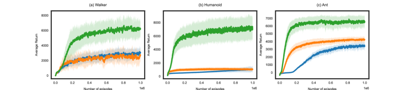
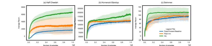
Figure 3: Empirical results averaged over 50 Monte Carlo runs with shaded regions showing the interquantile range.

5 Empirical evaluation

Through our experiments, we seek to answer the following questions: (1) Can history-based feature representation policies help improve the quality solution found by a memory-less RL algorithm? (2) In regards to the solution quality and sample complexity, how does the proposed method compare with other memory-augmented policies? (3) How does the choice of IPM affect the algorithms performance?

We answer question (1) and (2) by comparing our approach with the proximal policy gradient (PPO) algorithm which uses feed-forward neural networks. For question (2), we compare our method with an LSTM-based PPO variant which learns the feature representation using the history of states $S_{1:T}$ in a trajectory. For question (3) we compare the performance of our method using different MMD kernels and KL-divergence based approximation of Wasserstein distance. All the approaches are evaluated on six continuous control tasks from the MuJoCo [Todorov2012MuJoCoAP] OpenAI-Gym suite. To ensure a fair comparison, the baselines and their respective hyper-parameter settings are taken from well tested stand-alone implementations provided by baselines. From an implementation perspective, our framework can be used to modify any off-the-shelf policy-gradient algorithm by simply replacing (or augmenting) the feature abstraction layers of the policy and/or value networks with recurrent neural networks (RNNs), trained with the appropriate losses, as outlined previously. In these experiments, we replace the fully connected layers in PPO’s architecture with a Gated Recurrent Unit (GRU). For all the implementations, we initialise the hidden state of the GRU to zero at the beginning of the trajectory. This strategy simplifies the implementation and also allows for independent decorrelated sampling of sequences, therefore ensuring robust optimisation of the networks [rnn-hausknecht]. It is important to note that we can extend our framework to other policy gradient methods such as SAC [HaarnojaZAL18], TD3 [td3] or DDPG [ddpg], after satisfying certain technical conditions. However, we leave these extensions for future work. Additional experimental details and results can be found in Appendix E.

Fig. 3 contains the results of our experiments averaged over 50 Monte-Carlo evaluations using MMD-based AIS loss in (18). These results show that our algorithm improves over the performance of both the baselines, and the performance gain is significantly higher for high-dimensional environments like Humanoid and Ant. It is worth noticing that the GRU baseline also outperforms the feed-forward baseline for most environments. Overall, these findings lend credence to history-based encoding policies as a way to improve the quality of the solution learnt by the RL algorithm.

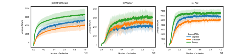
Figure 4: Comparison of different MMDs, averaged over 50 runs

Note that the MMD distance given by (48) in Subsection D.1.1, can be computed using different types of characteristic kernels (for a detailed review see  [Sriperumbudur, NIPS2009_685ac8ca, sejdinovic]). In this paper we consider computing (48) using the Laplace, Gaussian and energy distance kernels. In in Fig. 4 we compre the perfromance of our methods under different MMD kernels. It can be observed that for the continuous control tasks in the MuJoCo suite, the energy distance yields better performance, and therefore we implement Equation 48 using the energy distance for the results in Fig. 3.

Next, we compare the performance of our method under MMD (Energy distance kernel) and Wasserstein distance. From Fig. 5 we observe that for continuous control tasks, use of MMDs result in better performance as compared to Wasserstein distance.

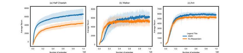
Figure 5: Comparison of Wasserstein vs MMDs, averaged over 50 runs.

6 Related Work

The development of RL algorithms with memory-based feature abstractions has been an active area of research, and most existing algorithms have tackled this problem using non-parametric methods like Nearest neighbour [Bentley1975MultidimensionalBS, Friedman1977AnAF, PENG1995438], Locally-weighted regression [Baird1993ReinforcementLW, locallyweighedatekson, Moore1997EfficientLW], and Kernel-based regression [Connell1987LearningTC, Dietterich2001BatchVF, kbrl, Xu2006KernelLT, Bhat2012NonparametricAD, BarretoAndr2016PracticalKR]. Despite their solid theoretical footing, these methods, have limited applicability as they are difficult to scale to high-dimensional state and action spaces. More recently, several methods that propose using recurrent neural networks for learning history-based abstractions have enjoyed considerable success in complex computer games [rnn-hausknecht, JaderbergMCSLSK17, impala, DBLP:conf/iclr/GruslysDAPBM18, ha] however most of these methods have been designed for partially observable environments where use of history-based methods is often necessary. To the best of our knowledge, the only other work where a history-based RL algorithm is used for controlling a MDP is presented by openai2019learning. In this work the authors show that using an LSTM-based agent architecture results in superior performance for the object reorientation using robotic arms. However, the authors do not provide a theoretical analysis of their method.

6.1 Bisimulation metrics

On the theoretical front, our work is closely related to state aggregation techniques based on bisimulation metrics proposed by Givan2003EquivalenceNA, Ferns2004MetricsFF, Ferns2011BisimulationMF. The bisimulation metric is the fixed point of an operator on the space of semi-metrics defined over the state space of an MDP with Lipschitz value functions. Apart from state aggregation, bisimulation metrics have been used for feature discovery [Comanici2011BasisFD, Ruan2015RepresentationDF], and transfer learning [Castro2010UsingBF]. However, computational impediments have prevented their broad adoption. Our work can be viewed as an alternative to bisimulation for the analysis of history-based state abstractions and deep RL methods. Our work can also be thought of as extension of the DeepMDP framework [deepmdp] to history-based policies and direct policy search methods.

6.2 AIS and Agent state

The notion of AIS is closely related to the epistemic state recently proposed by bvrstate. An epistemic state is a bounded representation of the history. It is updated recursively as the agent collects more information, and is represented as an environment proxy $\Upsilon$ which is learnt by optimising a target/objective function $\chi$. Since $\Upsilon$ is a random variable, its entropy $\mathbb{H}(\Upsilon)$ is used to represent system’s uncertainty about the environment. The framework proposed in this paper can considered as a practical way of constructing the system epistemic state where, the AIS $Z_{t}$ represents both the epistemic state and the environment proxy $\Upsilon$, $\mathcal{L}_{\text{AIS}}$ represents $\chi$, and instead of entropy, the constants $\epsilon$, and $\delta$ represent the systems uncertainty about the environment. The study of the AIS framework in the regret minimisation paradigm could help establish a relationship between the $\epsilon$, $\delta$, and $\mathbb{H}(\Upsilon)$, thereby helping designers develop principled algorithms which synthesise ideas like information directed sampling for direct policy search algorithms.

6.3 Analysis of RL algorithms with attention mechanism

Recently, there has been considerable interest in developing RL algorithms which use attention mechanism/transformer architectures [BahdanauCB14, Xu2015ShowAA] for learning feature abstractions [Zambaldi2019DeepRL, Mott2019TowardsIR, Sorokin2015DeepAR, Oh, RitterFSSBR21, ParisottoSRPGJJ20, chen, LoyndFcSH20, TangNH20, PritzelUSBVHWB17]. Attention mechanism extract task relevant information from historical observations and can be used instead of RNNs for processing sequential data [vaswani]. As we do not impose a functional from on the history compression function $\sigma_{t}(\cdot)$ in Definition 3.3, any attention mechanism can be interpreted as history compression function, and one can construct a valid information state by ensuring that the output of the attention mechanism satisfies (P1) and (P2). That being said, even without optimising $\mathcal{L}_{\text{AIS}}$, the approximation bound in Theorem 3.5 still applies for RL algorithms with attention mechanisms, with the caveat that the constants $\epsilon$, and $\delta$ may be arbitrarily large. A thorough empirical analysis of the effect of different attention mechanisms, and the AIS loss on the on the error constants $\epsilon$, and $\delta$ could help us gain a better understanding of the way in which such design choices could influence the learning process.

6.4 AIS for POMDPs

The concept of an AIS used in this paper is similar to the idea of AIS for POMDPs  [ais-2, ais-1]. Moreover, the literature also contains several other methods which have enjoyed empirical success in using history-based policies for controlling POMDPs [Isbell, hutte-1, hutter-2, Schaefer2007ARC, Dreamer, Pla-Net]. In principle, one can use any of these methods for controlling MDPs. However, this does not immediately provide a tight bound for the approximation error. The MDP model has more structure than POMDPs, and our goal in this paper is to use this fact to present a tighter analysis of the approximation error.

7 Conclusion and future work

This paper presents the design and analysis of a principled approach for learning history-based policies for controlling MDPs. We believe that our approximation bounds can be helpful for practitioners to study the effect of some of their design choices on the solution quality. On the practical side, the proposed algorithm shows favourable results on high-dimensional control tasks. Note that one can also use the bounds in Theorem 3.5 to analyse the approximation error of other history-based methods. However, since some of these algorithms do not satisfy Definition 3.3, the resulting approximation error might be arbitrarily large. Such blow-ups in the approximation error could be because the bound itself is loose or the optimality gap is large. This would depend on the specifics of the methods and remains to be investigated. As such, a sharper analysis of the approximation error by factoring in the specific design choices of other methods is an interesting direction for future research. Another interesting direction would be to conduct a thorough empirical evaluation exploring the design choices of history compression functions.

Appendix

Appendix A Proof for Theorem 3.5

For readability we will restate the theorem statement

Theorem A.1.

For any time $t$, any realisation $s_{t}$ of $S_{t}$, $a_{t}$ of $A_{t}$, let $h_{t}=(s_{1:t},a_{1:t-1})$, and $z_{t}=\sigma_{t}(h_{t})$. The worst case difference between $V^{\star}$ and $V^{\pi{}}_{t}$ is bounded as:

$$\Delta\leq 2\frac{\varepsilon+\gamma\delta\kappa_{\mathfrak{F}}(\hat{V}^{\mu},\hat{f})}{1-\gamma},$$ (25)

where, $\kappa_{\mathfrak{F}}(\hat{V},\hat{f})=\sup_{z,a}\rho_{\mathfrak{F}}(\hat{V}(\hat{f}(\cdot,z,a)))$. and $\rho_{\mathfrak{F}}(\cdot)$ is the Minkowski functional associated with the IPM $d_{\mathfrak{F}}$ as defined in (3).

Proof A.2.

For this proof we will use the following convention: For a generic history $h_{t}\in\mathcal{H}_{t}$, we assume that $h_{t}=(s_{1:t},a_{1:t-1})$, moreover, note that $z_{t}=\sigma_{t}(h_{t})$.

Now from (3.1), and Definition 3.3 for any $a_{t},s_{t},z_{t}$:

$$\max_{h\in\mathcal{H}_{t},a_{t}\in\mathcal{A}}\bigg{|}r(s_{t},a_{t})-\hat{r}(z_{t},a_{t})\bigg{|} \leq\epsilon.$$

$$\max_{h\in\mathcal{H}_{t},a_{t}\in\mathcal{A}}\bigg{|}\sum_{s_{t+1}\in\mathcal{S}}\bigg{(}P(s_{t+1}|s_{t},a_{t})\hat{V}^{\mu}(\hat{f}(s_{{}_{t}+1},z_{t},a_{t}))-\hat{P}(s_{t+1}|z_{t},a_{t})\hat{V}^{\mu}(\hat{f}(s_{t+1},z_{t},a_{t}))\bigg{)}\bigg{|} \leq\delta\rho_{\mathfrak{F}}(\hat{V}(\hat{f}(\cdot,z_{t},a_{t}))).$$ (26)

Now using triangle inequality we get:

$$\|V^{\star}(s_{t})-V_{t}^{\pi}(h_{t})\|_{\infty} \stackrel{{\scriptstyle(a)}}{{\leq}}\underbrace{\|V^{\star}(s_{t})-\hat{V}^{\mu}(z_{t})\|_{\infty}}_{\text{term 1}}+\underbrace{\|V_{t}^{\pi{}}(h_{t})-\hat{V}^{\mu}(z_{t})\|_{\infty}}_{\text{term 2}},$$ (27)

where $(a)$ follows from triangle inequality.

We will now proceed by bounding terms 1 and 2 separately

Bounding term 1:

$$\|V^{\star}(s_{t})-\hat{V}^{\mu}(z_{t})\|_{\infty} \leq\max_{h\in\mathcal{H}_{t}}\bigg{|}\max_{a_{t}\in\mathcal{A}}\bigg{[}Q^{\star}(s_{t},a_{t})-\hat{Q}^{\mu}(z_{t},a_{t})\bigg{]}\bigg{|},$$ (28)

Therefore, for any action $a_{t}$

$$\max_{h\in\mathcal{H}_{t}}\bigg{|}\max_{a_{t}\in\mathcal{A}}\bigg{[}Q^{\star}(s_{t},a_{t})-\hat{Q}^{\mu}(z_{t},a_{t})\bigg{]}\bigg{|} =\max_{h\in\mathcal{H}_{t}}\bigg{|}\max_{a_{t}\in\mathcal{A}}\bigg{[}r(s_{t},a_{t})+\gamma\sum_{s_{t+1}\in\mathcal{S}}P(s_{t+1}|s_{t},a_{t})V^{\star}(s_{t+1})$$

$$-\hat{r}(z_{t},a_{t})-\gamma\sum_{s_{t+1}\in\mathcal{S}}\hat{P}(s_{t+1}|z_{t},a_{t})\hat{V}^{\mu}(\hat{f}(s_{t+1},z_{t},a_{t}))\bigg{]}\bigg{|}$$

$$\stackrel{{\scriptstyle(a)}}{{\leq}}\epsilon+\max_{h\in\mathcal{H}_{t},a_{t}\in\mathcal{A}}\bigg{|}\gamma\sum_{s_{t+1}\in\mathcal{S}}P(s_{t+1}|s_{t},a_{t})V^{\star}(s_{t+1})-\gamma\sum_{s_{t+1}\in\mathcal{S}}P(s_{t+1}|s_{t},a_{t})\hat{V}^{\mu}(\hat{f}(s_{t+1},z_{t},a_{t}))\bigg{|}$$

$$+\max_{h\in\mathcal{H}_{t},a_{t}\in\mathcal{A}}\bigg{|}\gamma\sum_{s_{t+1}\in\mathcal{S}}P(s_{t+1}|s_{t},a_{t})\hat{V}^{\mu}(\hat{f}(s_{t+1},z_{t},a_{t}))-\gamma\sum_{s_{t+1}\in\mathcal{S}}\hat{P}(s_{t+1}|z_{t},a_{t})\hat{V}^{\mu}(\hat{f}(s_{t+1},z_{t},a_{t}))\bigg{|}$$

$$\stackrel{{\scriptstyle(b)}}{{\leq}}\epsilon+\gamma\|(V^{\star}(s_{t})-\hat{V}^{\mu}(z_{t}))\|_{\infty}+\gamma\delta\rho_{\mathfrak{F}}(\hat{V}^{\mu}(\hat{f}(\cdot,z_{t},a_{t}))),$$

where $(a)$ from triangle inequality and $(b)$ is due to (26). Now defining $\kappa_{\mathfrak{F}}(\hat{V},\hat{f})=\sup_{z,a}\rho_{\mathfrak{F}}(\hat{V}(\hat{f}(\cdot,z,a)))$, and substituting the above result in (28) we get

$$|V^{\star}(s_{t})-\hat{V}^{\mu}(z_{t})| \leq\frac{\varepsilon+\gamma\delta\kappa_{\mathfrak{F}}(\hat{V}^{\mu},\hat{f})}{1-\gamma}.$$ (29)

Bounding term 2:

$$\|V_{t}^{\pi{}}(h_{t})-\hat{V}^{\mu}(z_{t})\|_{\infty} \leq\max_{h\in\mathcal{H}_{t}}\bigg{|}\max_{a_{t}\in\mathcal{A}}\bigg{[}Q_{t}^{\pi{}}(h_{t},a_{t})-\hat{Q}^{\mu}(z_{t},a_{t})\bigg{]}\bigg{|},$$ (30)

Therefore, for any action $a_{t}$

$$\max_{h\in\mathcal{H}_{t}}\bigg{|}\max_{a_{t}\in\mathcal{A}}\bigg{[}Q^{\pi{}}(h_{t},a_{t})-\hat{Q}^{\mu}(z_{t},a_{t})\bigg{]}\bigg{|} =\max_{h\in\mathcal{H}_{t}}\bigg{|}\max_{a_{t}\in\mathcal{A}}\bigg{[}r(s_{t},a_{t})+\gamma\sum_{s_{t+1}\in\mathcal{S}}P(s_{t+1}|s_{t},a_{t})V_{t+1}^{\pi{}}(h_{t+1})$$

$$-\hat{r}(z_{t},a_{t})-\gamma\sum_{s_{t+1}\in\mathcal{S}}\hat{P}(s_{t+1}|z_{t},a_{t})\hat{V}^{\mu}(\hat{f}(s_{t+1},z_{t},a_{t}))\bigg{]}\bigg{|}$$

$$\stackrel{{\scriptstyle(a)}}{{\leq}}\epsilon+\max_{h\in\mathcal{H}_{t},a_{t}\in\mathcal{A}}\bigg{|}\gamma\sum_{s_{t+1}\in\mathcal{S}}P(s_{t+1}|s_{t},a_{t})V_{t+1}^{\pi{}}(h_{t+1})-\gamma\sum_{s_{t+1}\in\mathcal{S}}P(s_{t+1}|s_{t},a_{t})\hat{V}^{\mu}(\hat{f}(s_{t+1},z_{t},a_{t}))\bigg{|}$$

$$+\max_{h\in\mathcal{H}_{t},a_{t}\in\mathcal{A}}\bigg{|}\gamma\sum_{s_{t+1}\in\mathcal{S}}P(s_{t+1}|s_{t},a_{t})\hat{V}^{\mu}(\hat{f}(s_{t+1},z_{t},a_{t}))-\gamma\sum_{s_{t+1}\in\mathcal{S}}\hat{P}(s_{t+1}|z_{t},a_{t})\hat{V}^{\mu}(\hat{f}(s_{t+1},z_{t},a_{t}))\bigg{|}$$

$$\stackrel{{\scriptstyle(b)}}{{\leq}}\epsilon+\gamma\|(V^{\pi{}}(h_{t})-\hat{V}^{\mu}(z_{t}))\|_{\infty}+\gamma\delta\rho_{\mathfrak{F}}(\hat{V}^{\mu}(\hat{f}(\cdot,z_{t},a_{t}))),$$

where $(a)$ is from triangle inequality, $(b)$ is due to (26), with $\kappa_{\mathfrak{F}}(\hat{V},\hat{f})=\sup_{z,a}\rho_{\mathfrak{F}}(\hat{V}(\hat{f}(\cdot,z,a)))$, and substituting the above result in (30) we get

$$\|V^{\pi{}}_{t}(h_{t})-\hat{V}^{\mu}(z_{t})\|_{\infty} \leq\frac{\varepsilon+\gamma\delta\kappa_{\mathfrak{F}}(\hat{V}^{\mu},\hat{f})}{1-\gamma}.$$ (31)

The final result then follows by adding (29) and (31).

Appendix B Proof for Corollary 3.6

Lemma B.1.

If $\hat{V}$ is the optimal value function of the MDP $\hat{\mathcal{M}}$ induced by the process $\{Z_{t}\}_{t\geq 0}$, then

$$\operatorname{span}(\hat{V}) \leq\frac{\operatorname{span}(\hat{r})}{1-\gamma}.$$ (32)

Proof B.2.

The result follows by observing that the per-step reward $\hat{r}(Z_{t},A_{t})\in[\min(\hat{r}),\max(\hat{r})]$. Therefore $\max(\hat{V})\leq\max(\hat{r})$ and $\min(\hat{V})\geq\min(\hat{r})$.

Corollary B.3.

If the function class $\mathfrak{F}$ is $\mathfrak{F}^{\text{TV}}$, then $\Delta$ defined in (12) is upper bounded as:

$$\Delta\leq\frac{2\epsilon}{1-\gamma}+\frac{\gamma\delta\operatorname{span}(\hat{r})}{(1-\gamma)^{2}},$$ (33)

Proof B.4.

From 1. we know that for the Total variation distance $\rho_{\mathfrak{F}^{\text{TV}}}(\hat{V})$ = $\operatorname{span}(\hat{V})$ and $\kappa(\hat{f})=1$. The result in the corollary then follows from Lemma B.1.

Appendix C Proof for Corollary 3.7

Definition C.1.

For any Lipschitz function $f:(\mathcal{Z},d_{Z})\to(,|\cdot|)$, and probability measures $\nu_{1}$, and $\nu_{2}$ on $(\mathcal{Z},d_{Z})$

$$\bigg{|}\int_{\mathcal{Z}}fd\nu_{1}-\int_{\mathcal{Z}}fd\nu_{2}\bigg{|}\leq\|f\|_{L}.d_{\mathfrak{F}^{\text{W}}}(\nu_{1},\nu_{2})\leq L_{f}d_{\mathfrak{F}^{\text{W}}}(\nu_{1},\nu_{2}),$$ (34)

where $L_{f}$ is the Lipschitz constant of $f$ and $d_{\mathfrak{F}^{\text{W}}}$ is the Wasserstein distance.

Definition C.2.

Let $d$ be a metric on the AIS/Feature space $\mathcal{Z}$. The MDP $\hat{\mathcal{M}}$ induced by the process $\{Z_{t}\}_{t\geq 0}$ is said to be $(L_{\hat{r}},L_{\hat{P}})$ - Lipschitz if for any $Z_{1},Z_{2}\in\mathcal{Z}$, the reward $\hat{r}$ and transition $\hat{P}$ of $\hat{\mathcal{M}}$ satisfy the following:

$$\bigg{|}r(Z_{1},A)-r(Z_{2},A)\bigg{|} \leq L_{\hat{r}}d(Z_{1},Z_{2})$$ (35)

$$d_{\mathfrak{F}^{\text{W}}}(\hat{P}(\cdot|Z_{1},A),\hat{P}(\cdot|Z_{2},A) \leq L_{\hat{P}}d(Z_{1},Z_{2}),$$ (36)

where $d_{\mathfrak{F}^{\text{W}}}$ is the Wasserstein or the Kantorovitch-Rubinstein distance.

Lemma C.3.

Let $\hat{V}:\mathcal{Z}\to$ be $L_{\hat{V}}$ continuous. Define:

$$\hat{Q}(z,a) =\hat{r}(z,a)+\gamma\sum_{s^{\prime}}\hat{P}(s^{\prime}|z,a)\hat{V}(\hat{f}(s^{\prime},z,a).$$

Then $\hat{Q}$ is $(L_{\hat{r}}+\gamma L_{\hat{V}}L_{\hat{f}}L_{\hat{P}})$-Lipschitz continuous.

Proof C.4.

For any action $a$

$$\bigg{|}\hat{Q}(z_{1},a)-\hat{Q}(z_{2},a)\bigg{|} \stackrel{{\scriptstyle(a)}}{{\leq}}\bigg{|}\hat{r}(z_{1},a)-\hat{r}(z_{2},a)\bigg{|}+\gamma\bigg{|}\sum_{s^{\prime}}\hat{P}(s^{\prime}|z_{1},a)\hat{V}(\hat{f}(s^{\prime},z_{1},a))-\hat{P}(s^{\prime}|z_{2},a)\hat{V}(\hat{f}(s^{\prime},z_{2},a))\bigg{|}$$ (37)

$$\stackrel{{\scriptstyle(b)}}{{\leq}}(L_{\hat{r}}+\gamma L_{\hat{V}}L_{\hat{f}}L_{\hat{P}})d(z_{1},z_{2}),$$ (38)

where $(a)$ due to triangle inequality, and $(b)$ follows form Definition C.1, Definition C.2, and because $\|a\circ b\|_{L}\leq\|a\|_{L}\cdot\|b\|_{L}$.

Lemma C.5.

Let $\hat{Q}:\mathcal{Z}\times\mathcal{A}\to$ be $L_{\hat{Q}}$- Lipschitz continuous, Define

$$\hat{V}(z)=\max_{a_{t}\in\mathcal{A}}\hat{Q}(z,a).$$

Then $\hat{V}$ is $L_{\hat{Q}}$ Lipschitz

Proof C.6.

Consider $z_{1},z_{2}\in\mathcal{Z}$, and let $a_{1}$ and $a_{2}$ denote the corresponding optimal action. Then,

$$\hat{V}(z_{1})-\hat{V}(z_{2}) =\hat{Q}(z_{1},a_{1})-\hat{Q}(z_{2},a_{2})$$ (39)

$$\stackrel{{\scriptstyle(a)}}{{\leq}}\hat{Q}(z_{1},a_{2})-\hat{Q}(z_{2},a_{2})$$ (40)

$$\stackrel{{\scriptstyle(b)}}{{\leq}}L_{\hat{Q}}d(z_{1},z_{2}),$$ (41)

By symmetry,

$$\hat{V}(z_{2})-\hat{V}(z_{1}) \leq L_{\hat{Q}}d(z_{1},z_{2}).$$

Therefore,

$$\bigg{|}\hat{V}(z_{1})-\hat{V}(z_{2})\bigg{|} \leq L_{\hat{Q}}d(z_{1},z_{2}).$$

Lemma C.7.

Consider the following dynamic program defined in (8):

$$\hat{Q}_{t}(z_{t},a_{t}) =\hat{r}(z_{t},a_{t})+\gamma\sum_{s_{t}\in\mathcal{S}}\hat{P}(s_{t}|z_{t},a_{t})\hat{V}(\hat{f}(z_{t},s_{t},a_{t})),\ \forall z\in\mathcal{Z},a\in\mathcal{A}$$

$$\hat{V}_{t}(z_{t}) =\max_{a\in\mathcal{A}}\hat{Q}_{t}(z_{t},a_{t}),\ \forall z\in\mathcal{Z}$$

Then at any time $t$, we have:

$$L_{\hat{V}_{t+1}} =L_{\hat{r}}+\gamma L_{\hat{P}}L_{\hat{f}}L_{\hat{V}_{t}}.$$

Proof C.8.

We prove this by induction. At time $t=1$ $\hat{Q}_{1}(z,a)=\hat{r}(z,a)$, therefore $L_{\hat{Q}_{1}}=L_{\hat{r}}$. Then according to Lemma C.5, $\hat{V}_{1}$ is Lipschitz with Lipschitz constant $L_{\hat{V}_{1}}=L_{\hat{Q}_{1}}=L_{\hat{r}}$. This forms the basis of induction. Now assume that at time $t$, $\hat{V}_{t}$ is $L_{\hat{V}_{t}}$- Lipschitz. By Lemma C.3 $\hat{Q}_{t+1}$ is $L_{\hat{r}}+\gamma L_{\hat{f}},L_{\hat{P}}L_{\hat{V}_{t}}$. Therefore by Lemma C.5, $\hat{V}_{(t+1)}$ is Lipschitz with constant:

$$L_{\hat{V}_{t+1}} =L_{\hat{r}}+\gamma L_{\hat{f}}L_{\hat{P}}L_{\hat{V}_{t}}.$$

Theorem C.9.

Given any $(L_{\hat{r}},L_{\hat{P}})$- Lipschitz MDP, if $\gamma L_{\hat{P}}L_{\hat{f}}\leq 1$, then the infinite horizon $\gamma$-discounted value function $\hat{V}$ is Lipschitz continuous with Lipschitz constant

$$L_{\hat{V}} =\frac{L_{\hat{r}}}{1-\gamma L_{\hat{f}}L_{\hat{P}}}.$$

Proof C.10.

Consider the sequence of $L_{t}=L_{\hat{V}_{t}}$ values. For simplicity write $\alpha=\gamma L_{\hat{P}}L_{\hat{f}}$. Then the sequence $\{L_{t}\}_{t\geq 1}$ is given by : $L_{1}=L_{\hat{r}}$ and for $t\geq 1$,

$$L_{t+1} =L_{\hat{r}}+\alpha L_{t},$$

Therefore,

$$L_{t} =L_{\hat{r}}+\alpha L_{\hat{r}}+\ldots+\alpha_{t+1}=\frac{1-\alpha^{t}}{1-\alpha}L_{\hat{r}}.$$

This sequence converges if $|\alpha|\leq 1$. Since $\alpha$ is non-negative, this is equivalent to $\alpha\leq 1$, which is true by hypothesis. Hence $L_{t}$ is a convergent sequence. At convergence, the limit $L_{\hat{V}}$ must satisfy the fixed point of the recursion relationship introduced in Lemma C.7, hence,

$$L_{\hat{V}} =L_{\hat{r}}+\gamma L_{\hat{f}}L_{\hat{P}}L_{\hat{V}}.$$

Consequently, the limit is equal to,

$$L_{\hat{V}}=\frac{L_{\hat{r}}}{1-\gamma L_{\hat{f}}L_{\hat{P}}}.$$

Corollary C.11.

If $\gamma L_{\hat{P}}L_{\hat{f}}\leq 1$ and the function class $\mathfrak{F}$ is $\mathfrak{F}^{\text{W}}$, then $\Delta$ as defined in (12) is upper bounded as:

$$\Delta\leq\frac{2\epsilon}{(1-\gamma)}+\frac{2\gamma\delta L_{\hat{r}}}{(1-\gamma)(1-\gamma L_{\hat{f}}L_{\hat{P}})},$$ (42)

Proof C.12.

The proof follows from the observation that for $d_{\mathfrak{F}^{\text{W}}}$, $\rho_{\mathfrak{F}^{\text{W}}}$ = $L_{\hat{V}}$, and then using the result from Theorem C.9.

Appendix D Algorithmic Details

D.1 Choice of an IPM:

D.1.1 MMD

One advantage of choosing $d_{\mathfrak{F}}$ as the MMD distance is that unlike the Wasserstein distance, its computation does not require solving an optimisation problem. Another advantage is that we can leverage some of their properties to further simplify our computation, as follows:

Proposition D.1 (Theorem 22  [sejdinovic]).

Let $\mathcal{X}\subseteq^{m}$, and $d_{\mathcal{X},p}:\mathcal{X}\times\mathcal{X}\to$ be a metric given by $d_{\mathcal{X},p}(x,x^{\prime})=\|x-x^{\prime}\|^{p}_{2}$, for $p\in(0,2]$. Let $k_{p}:\mathcal{X}\times\mathcal{X}\to$ be any kernel given:

$$k_{p}(x,x^{\prime}) =\frac{1}{2}(d_{\mathcal{X},p}(x,x_{0})+d_{\mathcal{X},p}(x^{\prime},x_{0})-d_{\mathcal{X},p}(x,x^{\prime})),$$ (43)

where $x_{0}\in\mathcal{X}$ is arbitrary, and let $\mathcal{U}_{p}$ be a RKHS kernel with kernel $k_{p}$ and $\mathfrak{F}_{p}=\{f\in\mathcal{U}_{p}:\|f\|_{\mathcal{U}_{p}}\geq 1\}$. Then for any distributions $\nu_{1}$, $\nu_{2}\in\Delta{\mathcal{X}}$, the IPM can be expressed as:

$$d_{\mathfrak{F}}(\nu_{1},\nu_{2}) =\bigg{(}\underset{\begin{subarray}{c}\end{subarray}}{\mathbb{E}}[d_{\mathcal{X},p}(X_{1},W_{1})]-\frac{1}{2}\underset{\begin{subarray}{c}\end{subarray}}{\mathbb{E}}[d_{\mathcal{X},p}(X_{1},X_{2})]-\frac{1}{2}\underset{\begin{subarray}{c}\end{subarray}}{\mathbb{E}}[d_{\mathcal{X},p}(W_{1},W_{2})]\bigg{)}^{\frac{1}{2}},$$ (44)

where $X_{1},X_{2}$, and $W_{1},W_{2}$ are i.i.d. samples from $\nu_{1}$ and $\nu_{2}$ respectively.

The main implication of Proposition D.1 is that, instead of using (44), for $p\in(0,2]$ we can use the following as a surrogate for $d_{\mathfrak{F}_{p}}$:

$$\int_{\mathcal{X}}\int_{\mathcal{X}}\|x_{1}-w_{1}\|_{2}^{p}\nu_{1}(dx_{1})\nu_{2}(dw_{1})-\frac{1}{2}\int_{\mathcal{X}}\int_{\mathcal{X}}\|w_{1}-w_{2}\|_{2}^{p}\nu_{2}(dw_{1})\nu_{2}(dw_{1}).$$ (45)

Moreover, according to Sriperumbudur for n identically and independently distributed (i.i.d) samples $\{X_{i}\}_{i=0}^{n}\sim\nu_{1}$ an unbiased estimator of (45) is given as:

$$\frac{1}{n}\sum_{i=1}^{n}\int_{\mathcal{X}}\|X_{i}-w_{1}\|_{2}^{p}\nu_{1}d(w_{1})-\frac{1}{2}\int_{\mathcal{X}}\int_{\mathcal{X}}\|w_{1}-w_{2}\|_{2}^{p}\nu_{1}(dw_{1})\nu_{2}(dw_{2}).$$ (46)

We implement a simplified version of the surrogate loss in (46) as follows:

Proposition D.2 ( [ais-1]).

Given the setup in Proposition D.1 and $p=2$, Let $\nu_{2}(\zeta)$ be a parametric distribution with mean $m$ and let $X\sim\nu_{1}$, then the gradient $\nabla_{\zeta}(m_{\zeta}-2X)^{\top}m_{\zeta}$ is an unbiased estimator of $\nabla_{\zeta}d_{\mathfrak{F}_{2}}(\alpha,\nu_{\zeta})^{2}$

Proof D.3.

Let $X_{1},X_{2}\sim\nu_{1}$, and $W_{1},W_{2}\sim\nu_{2}(\zeta)$

$$\therefore\nabla_{\zeta}d_{\mathfrak{F}_{2}}(\nu_{1},\nu_{2}(\zeta))^{2} =\nabla_{\zeta}\bigg{[}\underset{\begin{subarray}{c}\end{subarray}}{\mathbb{E}}\|X_{1}-W_{1}\|_{2}^{2}-\frac{1}{2}\underset{\begin{subarray}{c}\end{subarray}}{\mathbb{E}}\|X_{1}-X_{2}\|_{2}^{2}-\frac{1}{2}\underset{\begin{subarray}{c}\end{subarray}}{\mathbb{E}}\|W_{1}-W_{2}\|_{2}^{2}\bigg{]}$$ (47)

$$\stackrel{{\scriptstyle(a)}}{{=}}\nabla_{\zeta}\bigg{[}\underset{\begin{subarray}{c}\end{subarray}}{\mathbb{E}}\|W_{1}\|_{2}^{2}-2\underset{\begin{subarray}{c}\end{subarray}}{\mathbb{E}}\|X_{1}\|^{\top}\underset{\begin{subarray}{c}\end{subarray}}{\mathbb{E}}\|W_{1}\|\bigg{]},$$ (48)

where $(a)$ follows from the fact that $X$ does not depend on $\zeta$, which simplifies the implementation of the MMD distance.

In this way we can simplify the computation of $d_{\mathfrak{F}}$ using a parametric stochastic kernel approximator and MMD metric.

Note that when are trying to approximate a continuous distribution we can readily use the loss function (48) as long as the mean $m_{\zeta}$ of $\nu_{2}(\zeta)$ is given in closed form. The AIS loss is then given as:

$$\mathcal{L}_{\text{AIS}}(\zeta) =\frac{1}{T}\sum_{t=0}^{T}\bigg{(}\lambda(f_{\hat{r}}(Z_{t},A_{t};\zeta)-r(S_{t},A_{t}))^{2}+(1-\lambda)(m^{S_{t}}_{\zeta}-2S_{t})^{\top}m^{S_{t}}_{\zeta}\bigg{)},$$ (49)

where $m^{S_{t}}_{\zeta}$ is obtained using the from the transition approximator,  i.e., the mapping $f_{\hat{P}}(\zeta):\mathcal{Z}\times\mathcal{A}\to$.

D.1.2 Wasserstein Distance

The the KL-divergence between two densities $\nu_{1}$ and $\nu_{2}$ on for any $X\in\mathcal{X}\subset^{m}$ is defined as:

$$d_{\text{KL}}(\nu_{1}\|\nu_{2}) =\int_{\mathcal{X}}\log(\nu_{1}(x))\nu_{1}(dx)-\int_{\mathcal{X}}\log(\nu_{2}(x))\nu_{1}(dx)$$ (50)

Moreover, if $\mathcal{X}$ is bounded space with diameter $D$, then the relation between the Wasserstein distance $d_{\mathfrak{F}^{\text{W}}}$, Total variation distance $d_{\mathfrak{F}^{\text{TV}}}$, and the KL divergence is given as :

$$d_{\mathfrak{F}^{\text{W}}}(\nu_{1},\nu_{2})\leq Dd_{\mathfrak{F}^{\text{TV}}}(\nu_{1},\nu_{2})\stackrel{{\scriptstyle(a)}}{{\leq}}\sqrt{2d_{\text{KL}}(\nu_{1}\|\nu_{2})},$$ (51)

where, $(a)$ follows from the Pinsker’s inequality. Note that in (17) we use $d_{\mathfrak{F}}^{2}$. Therefore, we can use a (simplified) KL-divergence based surrogate objective given as:

$$\int_{\mathcal{X}}\log(\nu_{2}(x;\zeta))\nu_{1}(dx),$$ (52)

where we have dropped the terms which do not depend on $\zeta$. Note that the above expression is same as the cross entropy between $\nu_{1}$ and $\nu_{2}$ which can be effectively computed using samples. In particular, if we get $T$ i.i.d samples from $\nu_{1}$, then,

$$\frac{1}{T}\sum_{i=0}^{T}\log(\nu_{2}(x_{i};\zeta))$$ (53)

is an unbiased estimator of $\int_{\mathcal{X}}\log(\nu_{2}(x;\zeta))\nu_{1}(dx)$.

The KL divergence based AIS loss is then given as:

$$\mathcal{L}_{\text{AIS}}(\zeta) =\frac{1}{T}\sum_{t=0}^{T}\bigg{(}\lambda(f_{\hat{r}}(Z_{t},A_{t};\zeta)-r(S_{t},A_{t}))^{2}+(1-\lambda)\log(\hat{P}(S_{t};\zeta))\bigg{)},$$ (54)

Appendix E Experimental Details

Common	Optimiser	Adam
	Discount Factor $\gamma$	0.99
	Inital standard deviation for the policy	0.0
	PPO-Epochs	12
	Clipping Coefficient	0.2
	Entropy-Regulariser	0
	Batch Size	512
	Episode Length	2048
AIS generator	History Compressor	GRU
	Hidden layer dimension	256
	Step size	1.5e-3
	$\lambda$	0.3
Actor	Step size	3.5e-4
	No of hidden layers	1
	Hidden layer Dimension	32

Table 1: Hyperparameters

E.1 Environments

Our algorithms are evaluated on MuJoCo [Todorov2012MuJoCoAP, mujoco-py version 2.0.2.9 ] via OpenAI gym [gym, version 0.17.1] interface, using the v2 environments. The environment, state-space, action space, and reward function are not modified or pre-processed in any way for easy reproducibility and fair comparison with previous results. Each environment runs for a maximum of 2048 time steps or until some termination condition and has a multi-dimensional action space with values in the range of (-1, 1), except for Humanoid which uses the range of (-0.4, 0.4).

E.2 Hyper-parameters

Table 1 contains all the hyper-parameters used in our experiments. Both the policy and AIS networks are trained with Adam optimiser [adam], with a batch size of 512. We follow Raichuk2021WhatMF’s recommended protocol for training on-policy policy based methods, and perform 12 PPO updates after every policy evaluation subroutine. To ensure separation of time-scales the step size of the AIS generator and the policy network is set to $1.5\text{e}^{-3}$ and $3.5\text{e}^{-4}$ respectively. Hyper-parameters of our approach are searched over a grid of values, but an exhaustive grid search is not carried out due to prohibitive computational cost. We start with the recommended hyper-parameters for the baseline implementations and tune them further around promising values by an iterative process of performing experiments and observing results.

For the state-based RNN baseline we have tuned the learning rate over a grid of values starting from 1e-4 to 4e-4 and settled on 3.5e-4 as it achieved the best performance. Similarly the hidden layer size set to 256 as it is observed to achieve best performance. For the feed-forward baselines we use the implementation by OpenAI baselines [baselines] with their default hyper-parameters.

References

- Atkeson et al. [1997] C. G. Atkeson, A. W. Moore, and S. Schaal. Locally Weighted Learning, pages 11–73. Springer Netherlands, Dordrecht, 1997. ISBN 978-94-017-2053-3. 10.1007/978-94-017-2053-3_2. URL https://doi.org/10.1007/978-94-017-2053-3_2.
- Bahdanau et al. [2015] D. Bahdanau, K. Cho, and Y. Bengio. Neural machine translation by jointly learning to align and translate. In Y. Bengio and Y. LeCun, editors, 3rd International Conference on Learning Representations, ICLR 2015, San Diego, CA, USA, May 7-9, 2015, Conference Track Proceedings, 2015. URL http://arxiv.org/abs/1409.0473.
- Baird and Klopf [1993] L. C. Baird and A. H. Klopf. Reinforcement learning with high-dimensional, continuous actions. Technical report, Wright Laboratory, 1993.
- Barreto et al. [2016] A. Barreto, P. Doina, and P. Joelle. Practical kernel-based reinforcement learning. Journal of Machine Learning Research, 2016.
- Barto et al. [2004] A. Barto, C. Anderson, and R. Sutton. Synthesis of nonlinear control surfaces by a layered associative search network. Biological Cybernetics, 43:175–185, 2004.
- Baxter and Bartlett [2001] J. Baxter and P. L. Bartlett. Infinite-horizon policy-gradient estimation. J. Artif. Intell. Res., 15:319–350, 2001. 10.1613/jair.806. URL https://doi.org/10.1613/jair.806.
- Bellemare et al. [2019] M. G. Bellemare, W. Dabney, R. Dadashi, A. A. Taïga, P. S. Castro, N. L. Roux, D. Schuurmans, T. Lattimore, and C. Lyle. A geometric perspective on optimal representations for reinforcement learning. In H. M. Wallach, H. Larochelle, A. Beygelzimer, F. d’Alché-Buc, E. B. Fox, and R. Garnett, editors, Advances in Neural Information Processing Systems 32: Annual Conference on Neural Information Processing Systems 2019, NeurIPS 2019, December 8-14, 2019, Vancouver, BC, Canada, pages 4360–4371, 2019. URL https://proceedings.neurips.cc/paper/2019/hash/3cf2559725a9fdfa602ec8c887440f32-Abstract.html.
- Bentley [1975] J. L. Bentley. Multidimensional binary search trees used for associative searching. Commun. ACM, 18:509–517, 1975.
- Bertsekas and Tsitsiklis [1996] D. P. Bertsekas and J. N. Tsitsiklis. Neuro-Dynamic Programming. Athena Scientific, 1st edition, 1996. ISBN 1886529108.
- Bhat et al. [2012] N. Bhat, C. C. Moallemi, and V. F. Farias. Non-parametric approximate dynamic programming via the kernel method. In NIPS, 2012.
- Borkar [2008] V. Borkar. Stochastic Approximation: A Dynamical Systems Viewpoint. Cambridge University Press, 2008. ISBN 9780521515924. URL https://books.google.ca/books?id=QLxIvgAACAAJ.
- Borkar [1997] V. S. Borkar. Stochastic approximation with two time scales. Systems & Control Letters, 29:291–294, 1997.
- Brockman et al. [2016] G. Brockman, V. Cheung, L. Pettersson, J. Schneider, J. Schulman, J. Tang, and W. Zaremba. Openai gym, 2016.
- Castro and Precup [2010] P. S. Castro and D. Precup. Using bisimulation for policy transfer in mdps. In AAAI, 2010.
- Chen et al. [2021] L. Chen, K. Lu, A. Rajeswaran, K. Lee, A. Grover, M. Laskin, P. Abbeel, A. Srinivas, and I. Mordatch. Decision transformer: Reinforcement learning via sequence modeling. CoRR, abs/2106.01345, 2021. URL https://arxiv.org/abs/2106.01345.
- Comanici and Precup [2011] G. Comanici and D. Precup. Basis function discovery using spectral clustering and bisimulation metrics. In AAAI, 2011.
- Connell and Utgoff [1987] M. E. Connell and P. Utgoff. Learning to control a dynamic physical system. Computational Intelligence, 3, 1987.
- Crites and Barto [1995] R. H. Crites and A. G. Barto. Improving elevator performance using reinforcement learning. In D. S. Touretzky, M. Mozer, and M. E. Hasselmo, editors, Advances in Neural Information Processing Systems 8, NIPS, Denver, CO, USA, November 27-30, 1995, pages 1017–1023. MIT Press, 1995. URL https://proceedings.neurips.cc/paper/1995/file/390e982518a50e280d8e2b535462ec1f-Paper.pdf.
- Daswani et al. [2013] M. Daswani, P. Sunehag, and M. Hutter. Q-learning for history-based reinforcement learning. In C. S. Ong and T. B. Ho, editors, Asian Conference on Machine Learning, ACML 2013, Canberra, ACT, Australia, November 13-15, 2013, volume 29 of JMLR Workshop and Conference Proceedings, pages 213–228. JMLR.org, 2013. URL http://proceedings.mlr.press/v29/Daswani13.html.
- Dhariwal et al. [2017] P. Dhariwal, C. Hesse, O. Klimov, A. Nichol, M. Plappert, A. Radford, J. Schulman, S. Sidor, Y. Wu, and P. Zhokhov. Openai baselines. https://github.com/openai/baselines, 2017.
- Dietterich and Wang [2001] T. G. Dietterich and X. Wang. Batch value function approximation via support vectors. In NIPS, 2001.
- Espeholt et al. [2018] L. Espeholt, H. Soyer, R. Munos, K. Simonyan, V. Mnih, T. Ward, Y. Doron, V. Firoiu, T. Harley, I. Dunning, S. Legg, and K. Kavukcuoglu. IMPALA: Scalable distributed deep-RL with importance weighted actor-learner architectures. In J. Dy and A. Krause, editors, Proceedings of the 35th International Conference on Machine Learning, volume 80 of Proceedings of Machine Learning Research, pages 1407–1416. PMLR, 10–15 Jul 2018. URL https://proceedings.mlr.press/v80/espeholt18a.html.
- Ferns et al. [2004] N. Ferns, P. Panangaden, and D. Precup. Metrics for finite markov decision processes. In Conferrence on Uncertainty in Artificial Intelligence, 2004.
- Ferns et al. [2011] N. Ferns, P. Panangaden, and D. Precup. Bisimulation metrics for continuous markov decision processes. SIAM J. Comput., 40:1662–1714, 2011.
- Friedman et al. [1977] J. H. Friedman, J. L. Bentley, and R. A. Finkel. An algorithm for finding best matches in logarithmic expected time. ACM Trans. Math. Softw., 3:209–226, 1977.
- Fujimoto et al. [2018] S. Fujimoto, H. van Hoof, and D. Meger. Addressing function approximation error in actor-critic methods. In J. G. Dy and A. Krause, editors, Proceedings of the 35th International Conference on Machine Learning, ICML 2018, Stockholmsmässan, Stockholm, Sweden, July 10-15, 2018, volume 80 of Proceedings of Machine Learning Research, pages 1582–1591. PMLR, 2018. URL http://proceedings.mlr.press/v80/fujimoto18a.html.
- Fukumizu et al. [2009] K. Fukumizu, A. Gretton, G. Lanckriet, B. Schölkopf, and B. K. Sriperumbudur. Kernel choice and classifiability for rkhs embeddings of probability distributions. In Y. Bengio, D. Schuurmans, J. Lafferty, C. Williams, and A. Culotta, editors, Advances in Neural Information Processing Systems, volume 22. Curran Associates, Inc., 2009. URL https://proceedings.neurips.cc/paper/2009/file/685ac8cadc1be5ac98da9556bc1c8d9e-Paper.pdf.
- Gelada et al. [2019] C. Gelada, S. Kumar, J. Buckman, O. Nachum, and M. G. Bellemare. Deepmdp: Learning continuous latent space models for representation learning. In K. Chaudhuri and R. Salakhutdinov, editors, Proceedings of the 36th International Conference on Machine Learning, ICML 2019, 9-15 June 2019, Long Beach, California, USA, volume 97 of Proceedings of Machine Learning Research, pages 2170–2179. PMLR, 2019. URL http://proceedings.mlr.press/v97/gelada19a.html.
- Givan et al. [2003] R. Givan, T. L. Dean, and M. Greig. Equivalence notions and model minimization in markov decision processes. Artif. Intell., 147:163–223, 2003.
- Gruslys et al. [2018] A. Gruslys, W. Dabney, M. G. Azar, B. Piot, M. G. Bellemare, and R. Munos. The reactor: A fast and sample-efficient actor-critic agent for reinforcement learning. In 6th International Conference on Learning Representations, ICLR 2018, Vancouver, BC, Canada, April 30 - May 3, 2018, Conference Track Proceedings. OpenReview.net, 2018. URL https://openreview.net/forum?id=rkHVZWZAZ.
- Ha and Schmidhuber [2018] D. Ha and J. Schmidhuber. World models. CoRR, abs/1803.10122, 2018. URL http://arxiv.org/abs/1803.10122.
- Haarnoja et al. [2018] T. Haarnoja, A. Zhou, P. Abbeel, and S. Levine. Soft actor-critic: Off-policy maximum entropy deep reinforcement learning with a stochastic actor. In J. G. Dy and A. Krause, editors, Proceedings of the 35th International Conference on Machine Learning, ICML 2018, Stockholmsmässan, Stockholm, Sweden, July 10-15, 2018, volume 80 of Proceedings of Machine Learning Research, pages 1856–1865. PMLR, 2018. URL http://proceedings.mlr.press/v80/haarnoja18b.html.
- Hafner et al. [2019] D. Hafner, T. P. Lillicrap, I. Fischer, R. Villegas, D. Ha, H. Lee, and J. Davidson. Learning latent dynamics for planning from pixels. In K. Chaudhuri and R. Salakhutdinov, editors, Proceedings of the 36th International Conference on Machine Learning, ICML 2019, 9-15 June 2019, Long Beach, California, USA, volume 97 of Proceedings of Machine Learning Research, pages 2555–2565. PMLR, 2019. URL http://proceedings.mlr.press/v97/hafner19a.html.
- Hafner et al. [2020] D. Hafner, T. P. Lillicrap, J. Ba, and M. Norouzi. Dream to control: Learning behaviors by latent imagination. In 8th International Conference on Learning Representations, ICLR 2020, Addis Ababa, Ethiopia, April 26-30, 2020. OpenReview.net, 2020. URL https://openreview.net/forum?id=S1lOTC4tDS.
- Hausknecht and Stone [2015] M. J. Hausknecht and P. Stone. Deep recurrent q-learning for partially observable mdps. In 2015 AAAI Fall Symposia, Arlington, Virginia, USA, November 12-14, 2015, pages 29–37. AAAI Press, 2015. URL http://www.aaai.org/ocs/index.php/FSS/FSS15/paper/view/11673.
- Holmes and Jr. [2006] M. P. Holmes and C. L. I. Jr. Looping suffix tree-based inference of partially observable hidden state. In W. W. Cohen and A. W. Moore, editors, Machine Learning, Proceedings of the Twenty-Third International Conference (ICML 2006), Pittsburgh, Pennsylvania, USA, June 25-29, 2006, volume 148 of ACM International Conference Proceeding Series, pages 409–416. ACM, 2006. 10.1145/1143844.1143896. URL https://doi.org/10.1145/1143844.1143896.
- Hutter [2014] M. Hutter. Extreme state aggregation beyond mdps. In P. Auer, A. Clark, T. Zeugmann, and S. Zilles, editors, Algorithmic Learning Theory - 25th International Conference, ALT 2014, Bled, Slovenia, October 8-10, 2014. Proceedings, volume 8776 of Lecture Notes in Computer Science, pages 185–199. Springer, 2014. 10.1007/978-3-319-11662-4_14. URL https://doi.org/10.1007/978-3-319-11662-4_14.
- Jaderberg et al. [2017] M. Jaderberg, V. Mnih, W. M. Czarnecki, T. Schaul, J. Z. Leibo, D. Silver, and K. Kavukcuoglu. Reinforcement learning with unsupervised auxiliary tasks. In 5th International Conference on Learning Representations, ICLR 2017, Toulon, France, April 24-26, 2017, Conference Track Proceedings. OpenReview.net, 2017. URL https://openreview.net/forum?id=SJ6yPD5xg.
- Keller et al. [2006] P. W. Keller, S. Mannor, and D. Precup. Automatic basis function construction for approximate dynamic programming and reinforcement learning. In Proceedings of the 23rd International Conference on Machine Learning, ICML ’06, page 449–456, New York, NY, USA, 2006. Association for Computing Machinery. ISBN 1595933832. 10.1145/1143844.1143901. URL https://doi.org/10.1145/1143844.1143901.
- Kingma and Ba [2015] D. P. Kingma and J. Ba. Adam: A method for stochastic optimization. CoRR, abs/1412.6980, 2015.
- Kullback and Leibler [1951] S. Kullback and R. A. Leibler. On Information and Sufficiency. The Annals of Mathematical Statistics, 22(1):79 – 86, 1951. 10.1214/aoms/1177729694. URL https://doi.org/10.1214/aoms/1177729694.
- Kwok and Fox [2004] C. Kwok and D. Fox. Reinforcement learning for sensing strategies. In 2004 IEEE/RSJ International Conference on Intelligent Robots and Systems (IROS) (IEEE Cat. No.04CH37566), volume 4, pages 3158–3163 vol.4, 2004. 10.1109/IROS.2004.1389903.
- Leslie [2004] D. Leslie. Reinforcement learning in games. 2004.
- Lillicrap et al. [2016] T. P. Lillicrap, J. J. Hunt, A. Pritzel, N. Heess, T. Erez, Y. Tassa, D. Silver, and D. Wierstra. Continuous control with deep reinforcement learning. In Y. Bengio and Y. LeCun, editors, 4th International Conference on Learning Representations, ICLR 2016, San Juan, Puerto Rico, May 2-4, 2016, Conference Track Proceedings, 2016. URL http://arxiv.org/abs/1509.02971.
- Loynd et al. [2020] R. Loynd, R. Fernandez, A. Celikyilmaz, A. Swaminathan, and M. J. Hausknecht. Working memory graphs. In Proceedings of the 37th International Conference on Machine Learning, ICML 2020, 13-18 July 2020, Virtual Event, volume 119 of Proceedings of Machine Learning Research, pages 6404–6414. PMLR, 2020. URL http://proceedings.mlr.press/v119/loynd20a.html.
- Lu et al. [2021] X. Lu, B. V. Roy, V. Dwaracherla, M. Ibrahimi, I. Osband, and Z. Wen. Reinforcement learning, bit by bit. CoRR, abs/2103.04047, 2021. URL https://arxiv.org/abs/2103.04047.
- Menache et al. [2005] I. Menache, S. Mannor, and N. Shimkin. Basis function adaptation in temporal difference reinforcement learning. Ann. Oper. Res., 134(1):215–238, 2005. 10.1007/s10479-005-5732-z. URL https://doi.org/10.1007/s10479-005-5732-z.
- Moore et al. [1997] A. W. Moore, J. G. Schneider, and K. Deng. Efficient locally weighted polynomial regression predictions. In ICML, 1997.
- Mott et al. [2019] A. Mott, D. Zoran, M. Chrzanowski, D. Wierstra, and D. J. Rezende. Towards interpretable reinforcement learning using attention augmented agents. In NeurIPS, 2019.
- Müller [1997] A. Müller. Integral probability metrics and their generating classes of functions. Advances in Applied Probability, 29(2):429–443, 1997. ISSN 00018678. URL http://www.jstor.org/stable/1428011.
- Oh and Kaneko [2018] H. Oh and T. Kaneko. Deep recurrent q-network with truncated history. In 2018 Conference on Technologies and Applications of Artificial Intelligence (TAAI), pages 34–39, 2018. 10.1109/TAAI.2018.00017.
- OpenAI et al. [2019] OpenAI, M. Andrychowicz, B. Baker, M. Chociej, R. Jozefowicz, B. McGrew, J. Pachocki, A. Petron, M. Plappert, G. Powell, A. Ray, J. Schneider, S. Sidor, J. Tobin, P. Welinder, L. Weng, and W. Zaremba. Learning dexterous in-hand manipulation, 2019.
- Ormoneit and Sen [2002] D. Ormoneit and S. Sen. Kernel-based reinforcement learning. Mach. Learn., 49(2-3):161–178, 2002. 10.1023/A:1017928328829. URL https://doi.org/10.1023/A:1017928328829.
- Parisotto et al. [2020] E. Parisotto, H. F. Song, J. W. Rae, R. Pascanu, Ç. Gülçehre, S. M. Jayakumar, M. Jaderberg, R. L. Kaufman, A. Clark, S. Noury, M. Botvinick, N. Heess, and R. Hadsell. Stabilizing transformers for reinforcement learning. In Proceedings of the 37th International Conference on Machine Learning, ICML 2020, 13-18 July 2020, Virtual Event, volume 119 of Proceedings of Machine Learning Research, pages 7487–7498. PMLR, 2020. URL http://proceedings.mlr.press/v119/parisotto20a.html.
- Peng [1995] J. Peng. Efficient memory-based dynamic programming. In A. Prieditis and S. Russell, editors, Machine Learning Proceedings 1995, pages 438–446. Morgan Kaufmann, San Francisco (CA), 1995. ISBN 978-1-55860-377-6. https://doi.org/10.1016/B978-1-55860-377-6.50061-X. URL https://www.sciencedirect.com/science/article/pii/B978155860377650061X.
- Petrik [2007] M. Petrik. An analysis of laplacian methods for value function approximation in mdps. In M. M. Veloso, editor, IJCAI 2007, Proceedings of the 20th International Joint Conference on Artificial Intelligence, Hyderabad, India, January 6-12, 2007, pages 2574–2579, 2007. URL http://ijcai.org/Proceedings/07/Papers/414.pdf.
- Pritzel et al. [2017] A. Pritzel, B. Uria, S. Srinivasan, A. P. Badia, O. Vinyals, D. Hassabis, D. Wierstra, and C. Blundell. Neural episodic control. In D. Precup and Y. W. Teh, editors, Proceedings of the 34th International Conference on Machine Learning, ICML 2017, Sydney, NSW, Australia, 6-11 August 2017, volume 70 of Proceedings of Machine Learning Research, pages 2827–2836. PMLR, 2017. URL http://proceedings.mlr.press/v70/pritzel17a.html.
- Proper and Tadepalli [2006] S. Proper and P. Tadepalli. Scaling model-based average-reward reinforcement learning for product delivery. In J. Fürnkranz, T. Scheffer, and M. Spiliopoulou, editors, Machine Learning: ECML 2006, 17th European Conference on Machine Learning, Berlin, Germany, September 18-22, 2006, Proceedings, volume 4212 of Lecture Notes in Computer Science, pages 735–742. Springer, 2006. 10.1007/11871842_74. URL https://doi.org/10.1007/11871842_74.
- Raichuk et al. [2021] A. Raichuk, P. Stanczyk, M. Orsini, S. Girgin, R. Marinier, L. Hussenot, M. Geist, O. Pietquin, M. Michalski, and S. Gelly. What matters for on-policy deep actor-critic methods? a large-scale study. In ICLR, 2021.
- Ritter et al. [2021] S. Ritter, R. Faulkner, L. Sartran, A. Santoro, M. Botvinick, and D. Raposo. Rapid task-solving in novel environments. In 9th International Conference on Learning Representations, ICLR 2021, Virtual Event, Austria, May 3-7, 2021. OpenReview.net, 2021. URL https://openreview.net/forum?id=F-mvpFpn_0q.
- Ruan et al. [2015] S. S. Ruan, G. Comanici, P. Panangaden, and D. Precup. Representation discovery for mdps using bisimulation metrics. In AAAI, 2015.
- Schaefer et al. [2007] A. Schaefer, S. Udluft, and H.-G. Zimmermann. A recurrent control neural network for data efficient reinforcement learning. 2007 IEEE International Symposium on Approximate Dynamic Programming and Reinforcement Learning, pages 151–157, 2007.
- Sejdinovic et al. [2013] D. Sejdinovic, B. Sriperumbudur, A. Gretton, and K. Fukumizu. Equivalence of distance-based and rkhs-based statistics in hypothesis testing. The Annals of Statistics, 41(5):2263–2291, 2013. ISSN 00905364, 21688966. URL http://www.jstor.org/stable/23566550.
- Singh et al. [2002] S. P. Singh, D. J. Litman, M. J. Kearns, and M. A. Walker. Optimizing dialogue management with reinforcement learning: Experiments with the njfun system. J. Artif. Intell. Res., 16:105–133, 2002. 10.1613/jair.859. URL https://doi.org/10.1613/jair.859.
- Sorokin et al. [2015] I. Sorokin, A. Seleznev, M. Pavlov, A. Fedorov, and A. Ignateva. Deep attention recurrent q-network. ArXiv, abs/1512.01693, 2015.
- Sriperumbudur et al. [2012] B. K. Sriperumbudur, K. Fukumizu, A. Gretton, B. Schölkopf, and G. R. G. Lanckriet. On the empirical estimation of integral probability metrics. Electronic Journal of Statistics, 6(none):1550 – 1599, 2012. 10.1214/12-EJS722. URL https://doi.org/10.1214/12-EJS722.
- Subramanian and Mahajan [2019] J. Subramanian and A. Mahajan. Approximate information state for partially observed systems. In 2019 IEEE 58th Conference on Decision and Control (CDC), pages 1629–1636, 2019. 10.1109/CDC40024.2019.9029898.
- Subramanian et al. [2020] J. Subramanian, A. Sinha, R. Seraj, and A. Mahajan. Approximate information state for approximate planning and reinforcement learning in partially observed systems. CoRR, abs/2010.08843, 2020. URL https://arxiv.org/abs/2010.08843.
- Sutton and Barto [1998] R. S. Sutton and A. G. Barto. Reinforcement Learning: An Introduction. MIT Press, Cambridge, MA, USA, 1998. ISBN 0-262-19398-1. URL http://www.cs.ualberta.ca/%7Esutton/book/ebook/the-book.html.
- Sutton and Barto [2018] R. S. Sutton and A. G. Barto. Reinforcement Learning: An Introduction. MIT Press, Cambridge, MA, USA, 2018.
- Sutton et al. [1999] R. S. Sutton, D. A. McAllester, S. P. Singh, and Y. Mansour. Policy gradient methods for reinforcement learning with function approximation. In S. A. Solla, T. K. Leen, and K. Müller, editors, Advances in Neural Information Processing Systems 12, [NIPS Conference, Denver, Colorado, USA, November 29 - December 4, 1999], pages 1057–1063. The MIT Press, 1999. URL https://proceedings.neurips.cc/paper/1999/file/464d828b85b0bed98e80ade0a5c43b0f-Paper.pdf.
- Tang et al. [2020] Y. Tang, D. Nguyen, and D. Ha. Neuroevolution of self-interpretable agents. In C. A. C. Coello, editor, GECCO ’20: Genetic and Evolutionary Computation Conference, Cancún Mexico, July 8-12, 2020, pages 414–424. ACM, 2020. 10.1145/3377930.3389847. URL https://doi.org/10.1145/3377930.3389847.
- Todorov et al. [2012] E. Todorov, T. Erez, and Y. Tassa. Mujoco: A physics engine for model-based control. 2012 IEEE/RSJ International Conference on Intelligent Robots and Systems, pages 5026–5033, 2012.
- Tsitsiklis and Roy [1996] J. N. Tsitsiklis and B. V. Roy. Feature-based methods for large scale dynamic programming. Mach. Learn., 22(1-3):59–94, 1996. 10.1023/A:1018008221616. URL https://doi.org/10.1023/A:1018008221616.
- Vaswani et al. [2017] A. Vaswani, N. Shazeer, N. Parmar, J. Uszkoreit, L. Jones, A. N. Gomez, L. u. Kaiser, and I. Polosukhin. Attention is all you need. In I. Guyon, U. V. Luxburg, S. Bengio, H. Wallach, R. Fergus, S. Vishwanathan, and R. Garnett, editors, Advances in Neural Information Processing Systems, volume 30. Curran Associates, Inc., 2017. URL https://proceedings.neurips.cc/paper/2017/file/3f5ee243547dee91fbd053c1c4a845aa-Paper.pdf.
- Williams [2004] R. J. Williams. Simple statistical gradient-following algorithms for connectionist reinforcement learning. Machine Learning, 8:229–256, 2004.
- Xu et al. [2015] K. Xu, J. Ba, R. Kiros, K. Cho, A. C. Courville, R. Salakhutdinov, R. S. Zemel, and Y. Bengio. Show, attend and tell: Neural image caption generation with visual attention. In ICML, 2015.
- Xu et al. [2006] X. Xu, T. Xie, D. Hu, and X. Lu. Kernel least-squares temporal difference learning. In Computational intelligence and neuroscience, 2006.
- Zambaldi et al. [2019] V. F. Zambaldi, D. Raposo, A. Santoro, V. Bapst, Y. Li, I. Babuschkin, K. Tuyls, D. P. Reichert, T. P. Lillicrap, E. Lockhart, M. Shanahan, V. Langston, R. Pascanu, M. M. Botvinick, O. Vinyals, and P. W. Battaglia. Deep reinforcement learning with relational inductive biases. In ICLR, 2019.